OPEN

ORIGINAL ARTICLE

Air quality monitoring using mobile microscopy andmachine learning

Yi-Chen Wu1,2,3, Ashutosh Shiledar1, Yi-Cheng Li1, Jeffrey Wong4, Steve Feng1,2,3, Xuan Chen1,Christine Chen1, Kevin Jin1, Saba Janamian1, Zhe Yang1, Zachary Scott Ballard1,2,3, Zoltán Göröcs1,2,3,Alborz Feizi1,2,3 and Aydogan Ozcan1,2,3,5

Rapid, accurate and high-throughput sizing and quantification of particulate matter (PM) in air is crucial for monitoring and

improving air quality. In fact, particles in air with a diameter of ≤2.5 μm have been classified as carcinogenic by the World

Health Organization. Here we present a field-portable cost-effective platform for high-throughput quantification of particulate

matter using computational lens-free microscopy and machine-learning. This platform, termed c-Air, is also integrated with a

smartphone application for device control and display of results. This mobile device rapidly screens 6.5 L of air in 30 s and gen-

erates microscopic images of the aerosols in air. It provides statistics of the particle size and density distribution with a sizing

accuracy of ~ 93%. We tested this mobile platform by measuring the air quality at different indoor and outdoor environments

and measurement times, and compared our results to those of an Environmental Protection Agency–approved device based on

beta-attenuation monitoring, which showed strong correlation to c-Air measurements. Furthermore, we used c-Air to map the air

quality around Los Angeles International Airport (LAX) over 24 h to confirm that the impact of LAX on increased PM concentra-

tion was present even at 47 km away from the airport, especially along the direction of landing flights. With its machine-

learning-based computational microscopy interface, c-Air can be adaptively tailored to detect specific particles in air, for exam-

ple, various types of pollen and mold and provide a cost-effective mobile solution for highly accurate and distributed sensing of

air quality.

Light: Science & Applications (2017) 6, e17046; doi:10.1038/lsa.2017.46; published online 8 September 2017

Keywords: air-quality monitoring; holography; machine learning; particulate matter

INTRODUCTION

Air quality is an increasing concern in the industrialized world.According to the World Health Organization (WHO), air pollutioncauses two million deaths annually in China, India and Pakistan.Moreover, ‘premature death’ of seven million people worldwide eachyear is due to the health hazards of air pollution1. Recently, severalsevere incidents of pollution haze afflicted Beijing, China and attractedworldwide attention2–4.Particulate matter (PM) is a mixture of solid and liquid particles in

air and forms a significant form of air pollution. PM sources include,for example, direct emission from a source, such as a construction site,smokestack, or fire, or a result of complex chemical reactions emittedfrom power plants, industrial production and automobiles5. PM witha general diameter of 10 μm and smaller, which is termed PM10,can cause serious health problems because it can become lodged deepin the lungs and even enter the bloodstream. A smaller PM sizecategory, PM2.5, which represents particles with a diameter of 2.5 μmor smaller, has been declared a cause of cancer by the WHO6.Furthermore, PM is a major environmental issue on account of

reduced visibility (haze). Monitoring PM air quality as a function ofspace and time is critical for understanding the effects of industrialactivities, studying atmospheric models and providing regulatory andadvisory guidelines for transportation, residents and industries.Currently, PM monitoring is performed at designated air sampling

stations, which are regulated by the US Environmental ProtectionAgency (EPA) and similar agencies in different countries. Manyof these advanced automatic platforms use either beta-attenuationmonitoring (BAM)7 or a tapered element oscillating microbalance(TEOM)7 instrument. BAM instruments sample aerosols on a rotatingfilter. Using a beta-particle source, they measure the beta-particleattenuation induced by the accumulated aerosols on the filter. TEOM-based instruments, on the other hand, capture aerosols in a filtercartridge, which contains a glass tube tip that vibrates at varyingfrequencies according to the mass of the captured aerosols. Thesedevices provide accurate PM measurements at high throughputs.However, they are cumbersome and heavy (~30 kg), relativelyexpensive (approximately $50 000–100 000) and require specializedpersonnel or technicians for regular system maintenance, for example,

1Electrical Engineering Department, University of California, Los Angeles, CA 90095, USA; 2Bioengineering Department, University of California, Los Angeles, CA 90095, USA;3California NanoSystems Institute (CNSI), University of California, Los Angeles, CA 90095, USA; 4Computer Science Department, University of California, Los Angeles, CA 90095,USA and 5David Geffen School of Medicine, University of California, Los Angeles, CA 90095, USACorrespondence: A Ozcan, Email: ozcan@ucla.edu, Web: http://innovate.ee.ucla.edu/Received 11 December 2016; revised 10 March 2017; accepted 11 March 2017; accepted article preview online 15 March 2017

Light: Science & Applications (2017) 6, e17046; doi:10.1038/lsa.2017.46Official journal of the CIOMP 2047-7538/17www.nature.com/lsa

every few weeks. Owing to these limitations, only ~ 10 000 of these airsampling stations exist worldwide.In addition to these high-end PM measurement instruments, several

commercially available portable particle counters are available at alower cost of approximately $2000 (Refs. 8,9) and in some cases muchhigher, approximately $7000–8000 (Ref. 10). These commerciallyavailable optical particle counters resemble a flow-cytometer. Theydrive the sampled air through a small channel. A laser beam focusedon the nozzle of this channel is scattered by each particle that passesthrough the channel. The scattering intensity is then used to inferthe particle size. Because of its serial read-out nature, the samplingrate of this approach is limited to o2–3 L �min�1 and in some sub-micron particle detection schemes o0.8 L �min�1 10. Furthermore,accurate measurement of either very-high or very-low concentrationsof particles is challenging for these devices, which limits the dynamicrange of the PM measurement. In addition to these limitations, thescattering cross-section, which comprises the quantity actually

measured by this device type, heavily depends on the three-dimensional (3D) morphology and refractive properties of theparticles. This can cause severe errors in the conversion of themeasured scattered light intensities into actual particle sizes. Finally,none of these designs offers a direct measure, that is, a microscopicimage of the captured particles, which is another limitation becausefurther analysis of a target particle of interest after its detection cannotbe performed.On account of these limitations, many air sampling activities

continue to use microscopic inspection and counting. Basically, airsamples are manually obtained in the field using a portable samplerthat employs various processes, such as cyclonic collection, impinge-ment, impaction, thermophoresis or filtering11–14. The sample is thensent to a central laboratory, where it is post-processed and manuallyinspected under a microscope by an expert. This type of microscopicanalysis provides the major advantage of more accurate particle sizing,while enabling the expert reader to recognize the particle shape and

D

a

b

c

d

Paritally coherentIllumination

Impactornozzle

Stickycoverslip

Imagesensor2 cm

E

C

A

B

Hologram Reconst.

30 µm

~800 µm

~400 µm

Hologram Reconst.

30 µm200 µm

e

Hologram Reconst.

30 µm

F

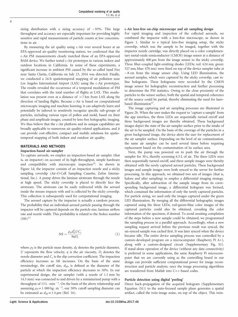
Figure 1 c-Air platform. (a and b) Photos of the device from different perspectives. A quarter is placed beside the device in b for scale. (c) 3D computer-aided-design (CAD)-drawing overview of the device, including (A) rechargeable battery, (B) vacuum pump (13 L �min�1), (C) illumination module with fiber-coupled light-emitting diodes of red (624 nm), green (527 nm) and blue (470 nm) and (D) impaction-based air sampler with (E) a sticky coverslip on top of(F) the image sensor. (d) Schematic drawing of impaction-based air sampler on a chip. (e) Whole field-of-view differential hologram image of an aerosolsample during sampling, and zoomed-in regions of its reconstruction. The device is powered by a rechargeable battery (A), and controlled by a microcontroller(Raspberry Pi A+). The assembly and packaging are 3D-printed.

Computational monitoring of air qualityY-C Wu et al

2

Light: Science & Applications doi:10.1038/lsa.2017.46

type. These capabilities yield additional benefits in more complicatedanalyses of air pollution, such as identification of a specific aerosoltype. In this method, however, the sampling and inspection processesare separated; that is, the sampling is performed in the field, whereasthe sample analysis is conducted in a remote professional lab. Thissignificantly delays the reporting of the results. Furthermore, theinspection is manually performed by a trained expert, which con-siderably increases the overall cost of each air-quality measurement.Furthermore, this conventional microscope-based screening of aero-sols cannot be conducted in the field, because these benchtopmicroscopes are cumbersome, heavy, expensive and require specializedskills to operate.In this paper, as a transformative solution to the above outlined

limitations of existing air quality measurement techniques, we presenta hand-held and cost-effective platform for automated sizing andhigh-throughput quantification of PM using computational lens-freemicroscopy and machine learning. As an alternative to conventional

lens-based microscopy techniques, in a computational lens-freemicroscopy approach, the sample is directly positioned on top of animage sensor chip with no optical components between them15,16.Such an on-chip microscope can rapidly reconstruct images oftransmissive samples over a very large field of view of 420 mm2.On the basis of this computational on-chip imaging concept and aunique machine learning enabled particle analysis method, wedemonstrate in this paper the design of a lightweight (~590 g),hand-held and cost-effective air-quality monitoring system, termedc-Air. This mobile system utilizes a micro-pump, an impaction-basedair-sampler and a lens-free holographic on-chip microscope that isintegrated with a custom-written machine learning algorithm forremote data processing and particle analysis. The c-Air platform(Figures 1 and 2) operates with a smartphone application (app) fordevice control and data display. It can rapidly screen 6.5 L of airvolume in 30 s, generating microscopic phase and amplitude images ofthe captured particles, while also automatically providing the PM

5. Syncimage toserver for

processing

a b

c

(i) (ii) (iii)

(i v) (v) (vi)

2. Takeback-

groundimages(R,G,B)

4. Takeraw sample

images(R,G,B)

1. Receivethe imageand GPSlocation

5. Transferand displayresults onthe phone

APP

4. Sizingand sizestatistics

3. Particledetection

usingpeeling & ML

2. Differentialimaging

3. Pump airfor 30 s at13 L min–1

Airsampler

Remote server

(Start)1. Phone

APP control

Figure 2 c-Air work flow and iOS-based app interface. (a) iOS-based c-Air app interface: (i) ‘Welcome’ screen of the app with different options. (ii) ‘TakeMeasurement’ screen with a device-logo-shaped sampling button. (iii) Changing the device connection. The user can change the device to be connected bytyping the IP address of the device. (iv) ‘Map View’ of history samples. The air samples can be viewed by touching the pinpoint. (v) ‘List View’ of historysamples. Each entry is a sample that shows the device name and capture time. (vi) View of one sample result. The ‘graph’ option shows a histogram of theparticle sizing. (b) Work flow on the c-Air device. (c) Workflow on the server to support the processing of air samples. After the sample image and GPSlocation are sent to the server, the server processes the images through all five stages and saves the processed result. A copy of the result is sent to thesmartphone app, where it is rendered and displayed. GPS, global position system; ML, machine learning.

Computational monitoring of air qualityY-C Wu et al

3

Light: Science & Applicationsdoi:10.1038/lsa.2017.46

sizing distribution with a sizing accuracy of ~ 93%. This largethroughput and accuracy are especially important for providing highlysensitive and rapid measurements of particle counts at low concentra-tions in air.By measuring the air quality using c-Air over several hours at an

EPA-approved air-quality monitoring station, we confirmed that thec-Air PM measurements closely matched those of an EPA-approvedBAM device. We further tested c-Air prototypes in various indoor andoutdoor locations in California. In some of these experiments, asignificant increase in ambient PM caused by the so-called Sand Firenear Santa Clarita, California on July 23, 2016 was detected. Finally,we conducted a 24-h spatiotemporal mapping of air pollution nearLos Angeles International Airport (LAX) using the c-Air prototypes.The results revealed the occurrence of a temporal modulation of PMthat correlates with the total number of flights at LAX. This modu-lation was present even at a distance of 47 km from LAX along thedirection of landing flights. Because c-Air is based on computationalmicroscopic imaging and machine learning, it can adaptively learn andpotentially be tailored to sensitively recognize specific sub-groups ofparticles, including various types of pollen and mold, based on theirphase and amplitude images, created by lens-free holographic imaging.We thus believe that the c-Air platform and its unique capabilities arebroadly applicable to numerous air-quality-related applications, and itcan provide cost-effective, compact and mobile solutions for spatio-temporal mapping of both indoor and outdoor air quality.

MATERIALS AND METHODS

Impaction-based air-samplerTo capture aerosols, we employ an impaction-based air sampler (thatis, an impactor) on account of its high-throughput, simple hardwareand compatibility with microscopic inspection15. As shown inFigure 1d, the impactor consists of an impaction nozzle and a stickysampling coverslip (Air-O-Cell Sampling Cassette, Zefon Interna-tional, Inc.). A pump drives the laminar airstream through the nozzleat high speed. The sticky coverslip is placed to directly face theairstream. The airstream can be easily redirected while the aerosolinside the stream impacts with and is collected by the sticky coverslip.This collection is subsequently used for computational imaging.The aerosol capture by the impactor is actually a random process.

The probability that an individual aerosol particle passing through theimpactor will be captured depends on the particle size, laminar airflowrate and nozzle width. This probability is related to the Stokes number(Stk):11

Stk ¼ rPd2PUCc

9ZDjð1Þ

where ρP is the particle mass density, dP denotes the particle diameter,U represents the flow velocity, η is the air viscosity, Dj denotes thenozzle diameter and Cc is the slip correction coefficient. The impactionefficiency increases as Stk increases. On the basis of the sameterminology, the cutoff size, d50, is defined as the diameter of theparticle at which the impaction efficiency decreases to 50%. In ourexperimental design, the air sampler (with a nozzle of 1.1 mm by14.5 mm) was connected to and driven by a miniaturized pump with athroughput of 13 L �min�1. On the basis of the above relationship andassuming ρP= 1 000 kg �m�3, our 50% cutoff sampling diameter canbe estimated as d50= 1.4 μm (Ref. 16).

c-Air lens-free on-chip microscope and air sampling designFor rapid imaging and inspection of the collected aerosols, wecombined the impactor with a lens-free microscope, as shown inFigure 1. Similar to a typical lens-free imaging setup, the stickycoverslip, which was the sample to be imaged, together with theimpactor nozzle cartridge, was directly placed on a color complemen-tary metal-oxide semiconductor (CMOS) image sensor at a distance ofapproximately 400 μm from the image sensor to the sticky coverslip.Three fiber-coupled light-emitting diodes (LEDs; red: 624 nm; green:527 nm; blue: 470 nm) were fixed on top of the device sampler tube at~ 8 cm from the image sensor chip. Using LED illumination, theaerosol samples, which were captured by the sticky coverslip, cast in-line holograms. These holograms were recorded by the CMOSimage sensor for holographic reconstruction and further processingto determine the PM statistics. Owing to the close proximity of theparticles to the sensor surface, both the spatial and temporal coherenceof the source could be partial, thereby eliminating the need for laser-based illumination17.The image capturing and air sampling processes are illustrated in

Figure 2b. When the user makes the request to ‘capture a sample’ fromthe app interface, the three LEDs are sequentially turned on/off andthree background images are thereby obtained. These backgroundimages depict the state of the air-sampler surface prior to the intake ofthe air to be sampled. On the basis of the coverage of the particles in agiven background image, the device alerts the user for replacement ofthe air sampler surface. Depending on the level of air contamination,the same air sampler can be used several times before requiringreplacement based on the contamination of its surface area.Next, the pump was powered on to push the air through the

sampler for 30 s, thereby screening 6.5 L of air. The three LEDs werethen sequentially turned on/off, and three sample images were therebyobtained with the newly captured aerosol particles. These backgroundimages and sample images were both synced to the server for furtherprocessing. In this approach, we obtained two sets of images (that is,before and after sampling) to employ a differential imaging strategy.Specifically, after subtraction of the sample image from its corre-sponding background image, a differential hologram was formed,which contained the information of only the newly captured particles.For particle sizing, we used only the images captured under the greenLED illumination. By merging all the differential holographic imagescaptured using the three LEDs, red–green–blue color images of thecaptured particles could also be obtained, revealing the colorinformation of the specimen, if desired. To avoid awaiting completionof the steps before a new sample could be obtained, we programmedthe sampling process in a parallel approach. Accordingly, when a newsampling request arrived before the previous result was synced, theun-synced sample was cached first. It was later synced when the devicebecame idle. The entire device sampling process was controlled by acustom-developed program on a microcomputer (Raspberry Pi A+),along with a custom-designed circuit (Supplementary Fig. S1).If stand-alone operation of the device (without any data connectivity)is preferred in some applications, the same Raspberry Pi microcom-puter that we are currently using as the controlling board in ourdesign can provide sufficient computational power for image recon-struction and particle analysis, once the image processing algorithmsare transferred from Matlab into C++-based codes.

Particle detection using digital ‘peeling’Direct back-propagation of the acquired hologram (SupplementaryEquation (S1)) to the auto-focused sample plane generates a spatialartifact, called the twin-image noise, on top of the object. This twin-

Computational monitoring of air qualityY-C Wu et al

4

Light: Science & Applications doi:10.1038/lsa.2017.46

image artifact affects the detection of aerosol particles. If leftunprocessed, it can lead to false-positives and false-negatives. Toaddress this problem, we employ an iterative particle peelingalgorithm18 in our holographic reconstruction process. It is addition-ally combined with a support vector machine (SVM)-based learningmodel to further reject these spatial artifacts. The algorithm issummarized as a flowchart in Supplementary Fig. S2.This peeling algorithm contains four cycles of detection and erasing

(‘peeling out’) of the particles at progressively increasing thresholds,that is, 0.75, 0.85, 0.92 and 0.97, where the background is centeredat 1.0 during the differential imaging process (SupplementaryInformation). The highest threshold (0.97) is selected as 3σ fromthe background mean, where σ≈ 0.01 is the s.d. of the background.We use a morphological reconstruction process19 to generate theimage mask instead of using a simple threshold. Because most particleshave a darker center and a somewhat weaker boundary, using a singlethreshold may mask parts of the particle, potentially causing theparticle to be missed or re-detected multiple times in subsequentpeeling cycles. This is avoided by using a morphological reconstructionprocess.In each cycle of this digital particle peeling process, we first adjust

the image focus using the auto-focusing algorithm (SupplementaryInformation). Then, a morphological reconstruction is employed togenerate a binary mask, where each masked area contains a particle.For each mask, we crop a small image (100× 100 pixels) and performfine auto-focusing on this small image to find the correct focus planeof the corresponding particle. At this focus plane, we extract variousspatial features of the particle, for example, minimum intensity Im,average intensity Ia, area A and maximum phase θM. We thenpropagate (using Supplementary Equation (S1)) the image to fivedifferent planes uniformly spaced between 20 μm above and 20 μmbelow this focus plane. The Tamura coefficient (see SupplementaryEquation (S3)) of this focus plane is calculated and compared to thecoefficients of these five other planes. The ratio of the Tamuracoefficient at this focus plane against the highest Tamura coefficient ofall six planes is defined as another feature, RTam. These four features,Im, θM, A and RTam, are then fed into an SVM-based learning model todigitally separate spatial artifacts from true particles and reject suchartifacts. This learning algorithm is detailed in the following sub-section. After all the detected particles in this peeling cycle areprocessed, we digitally peel out these ‘counted’ particles, that is,replace the thresholded area corresponding to each detected particlewith the background mean, on both the image and twin image planes.We then move to the next peeling cycle with a higher threshold andrepeat the same steps.After completing all four peeling cycles, the extracted features, Im,

θM and A, are further utilized for particle sizing using a machine-learning algorithm, as detailed further below. This sizing process isonly performed on true particles, which generates a histogram ofparticle sizes and density distributions, as well as various otherparameters, including, for example, total suspended particulate(TSP), PM10 and PM2.5, reported as part of c-Air result summary.

Elimination of false-positives using a trained support vectormachineTo further avoid false-positives in our detection system, we used atrained linear SVM that is based on four features, Im, θM, A and RTam,as described in the previous sub-section, to distinguish spatial artifactsfrom true particles and increase c-Air detection accuracy. These spatialfeatures were selected to provide the best separation between the true-and false-particles. To train this model, we obtained two air sample

images using a c-Air prototype, one indoor and one outdoor. Then, inaddition to our c-Air-based analysis, we physically extracted thesampling coverslip and inspected the captured particles under abenchtop bright-field microscope using a 40× objective lens. Wecompared the thresholded areas in our peeling cycle and lens-freereconstruction process with the images of the benchtop microscope tomark each one of these detected areas as a true particle or a false one.Using this comparison, we labeled a total of 42000 thresholded areasand fed half of this training data into our SVM model20 (implementedin Matlab using the function ‘svmtrain’). The other half was used forblind testing of the model, which showed a precision of 0.95 and arecall of 0.98.

Machine-learning-based particle detection and sizingWe used a custom-designed machine-learning algorithm trained onsize-calibrated particles to obtain a mapping from the detected spatialcharacteristics of the particles to their diameter, also helping us avoidfalse positives, false negatives as well as over-counting of movedparticles in our detection process. For this purpose, we used somespatial features extracted from the holographic particle images,including for example, minimum intensity Im, average intensity Iaand area A, and developed a second-order regression model that mapsthese features to the sizes of the detected particles in microns. Themodel is deterministically learned from size-labeled particle images,which are manually sized using a standard benchtop microscope.Specifically, after we extract features Im, Ia and A of the masked regionin a particle peeling cycle, we strive to find a model, f, that maps thesefeatures to the particle diameter D in microns, that is,

D ¼ f Im; Ia;ffiffiffiA

p� �ð2Þ

Where f can potentially have infinite dimensions. However, we employa simplified second-order polynomial model of f and extend thefeatures to the second-order by defining:

X ¼ 1; Im; Ia;ffiffiffiA

p; I2m; I

2a ;A; ImIa; Im

ffiffiffiA

p; Ia

ffiffiffiA

ph ið3Þ

We then define a linear mapping, θ, that relates the second-orderfeatures to the diameter of the particle:

D ¼ f Im; Ia;ffiffiffiA

p� �¼ yTX̂ ¼ yT

X � ms

� �ð4Þ

where T refers to the transpose operation, and μ and σ represent themean and s.d. of X, respectively.Based on the above mapping, we used 395 size-labeled microbeads

for training and blind testing. These polystyrene microbeads ranged indiameter from ~1 to ~ 40 μm, as shown in Figure 3. The ground truthsizes of these particles were manually measured under a benchtopmicroscope with a 100 ´ 0.95 numerical aperture (NA) objective lens.The same samples were additionally imaged using the c-Air platformto obtain the corresponding lens-free images and extract spatialfeatures, Im, θM and A. For training the machine-learning model, wefirst randomly and evenly separated the microbead samples intorespective training and testing sets. After extending the features to thesecond-order (Equation (3)) and performing normalization (Equation(4)), we fitted the parameter vector θ by minimizing the differencebetween the training feature mapping yTX̂ tr

� �and the calibrated

diameter Dmictr

� �that is,

miny8yT X̂ tr � Dmic

tr 81 ð5ÞThis minimization was performed by CVX, a software packagedesigned for solving convex optimization problems21. The same

Computational monitoring of air qualityY-C Wu et al

5

Light: Science & Applicationsdoi:10.1038/lsa.2017.46

trained parameter was then applied for the cross-validation set, whichwas comprised of another 197 microbeads. Particle sizing trainingerrors (Etr) and testing errors (Ecv) were validated by evaluating thenorm of difference:

Etr ¼ 8yT X̂ tr � Dmictr 8p ð6Þ

Ecv ¼ 8yT X̂ cv � Dmiccv 8p ð7Þ

where yTX̂ cv is the testing feature mapping, and Dmiccv is the calibrated

diameter for the testing set. In addition, p= 1 is used for calculatingthe ‘mean error,’ and p=∞ is used for calculating the ‘maximumerror.’ Note that this training process only needs to be done once, andthe trained parameter vector, θ and the normalization parameters,μ and σ, are then saved and subsequently used for blind particle sizingof all the captured aerosol samples using c-Air devices.

RESULTS AND DISCUSSION

C-Air platform spatial resolution, detection limit and field of viewThe USAF-1951 resolution test target was used to quantify the spatialresolution of the c-Air platform. The reconstructed image of this testtarget is shown in Supplementary Fig. S3, where the smallest resolvableline is group eight, element two (line width 1.74 μm), which iscurrently pixel-size limited due to our unit magnification imaginggeometry17,22. If required in future applications, a better resolution(for example,r 0.5 μm) can be achieved in our c-Air platform using aCMOS sensor with a small pixel size and/or by applying pixel super-resolution techniques to digitally synthesize smaller pixel sizes22–25.In our reconstructed lens-free differential images, we defined the

detection noise floor as 3σ (σ≈ 0.01 is the s.d. of the background)from the background mean, which is always 1 in a given normalizeddifferential image, as detailed in our Supplementary Information. Fora particle to be viewed as detected, its lens-free signal should be abovethis 3σ noise floor. As shown in Supplementary Fig. S4, 1 μm particlescan be clearly detected, which is also cross-validated by a benchtop

microscope comparison. We should note that, as desired, thisdetection limit is well below the 50% cut-off sampling diameter ofour impactor (d50= 1.4 μm, see the Materials and Methods section fordetails).In terms of the imaging field of view, the active area of the CMOS

sensor in our c-Air design is 3.67× 2.74= 10.06 mm2. However, in theimpactor air sampler geometry (Figure 1d), the particles are depositedimmediately below the impaction nozzle. Thus, the active area thatwill be populated by aerosols and imaged by the lens-free microscopewill be the intersection of the active area of the CMOS sensor andthe impaction nozzle opening. Because the slit has a width of only1.1 mm, the resulting effective imaging field of view of c-Air is3.67× 1.1= 4.04 mm2. With either the selection of a different CMOSimage sensor chip or a custom-developed impaction nozzle, the nozzleslit area and the image sensor area can have larger spatial overlaps tofurther increase this effective field of view in future c-Air designs.

Particle-sizing accuracy using machine learningAs detailed in the Materials and Methods section, we used a machine-learning algorithm trained on size-calibrated particles to obtain amapping from the detected spatial characteristics of the particles totheir diameter. Figure 3 depicts how well the predicted particlediameter, Dpred, based on our machine-learning algorithm describedin the Materials and Methods section, agrees with the ground-truthmeasured diameter, Dref. The sizing errors for training and testing setsare defined in Equations (6) and (7), respectively. The dotted blackline in Figure 3 represents the reference for Dref=Dpred. As shown inFigure 3, using machine learning, c-Air achieved an average sizingerror of ~ 7% for both the training and blind testing sets. For non-standard particles, for example, rod-shaped or arbitrarily shapedfibers, our microscopic imaging system will be able to determine thatthe above described size mapping will not be applicable. For thesenon-standard particles that are detected on our sampling surface, wecan characterize them using new parameters based on their

60Reference line Size 1 µm

37

0 10 20 30 40 50 60

2 µm

Mean error (µm)

Training set Testing set

Mean error (%)

0.2203 0.3565

Max error (µm)

6.0856 7.5031

Max error (%)

1.6481 11.7521

70.076758.3739

3 µm 4 µm 6 µm 10 µm 19 µm 42 µm

#

0 20Diameter (µm)

40 60

50 51 54 86 50 50 17Training setTesting set

5080

60

40

20

0

40

Pre

dict

ed d

iam

eter

- D

pred

(µm

)

Reference diameter - Dref (µm)

Aer

osol

cou

nt

30

20

10

0

Figure 3 Machine-learning-based particle detection and sizing with high accuracy using c-Air. The designated bead sizes are shown in the uppermost table.The microscope-calibrated size distribution is plotted as the histogram within the large figure. The large figure in the background shows the machine-learningmapped size (Dpred) using c-Air. It is compared to the microscope-measured size (Dref) for both training and testing sets. The middle dashed line representsDpred=Dref. The sizing error, which is defined by Equations (6) to (7), is shown in the lower-right table in both μm and the relative percentage. A ~93%accuracy using machine-learning-based sizing is demonstrated.

Computational monitoring of air qualityY-C Wu et al

6

Light: Science & Applications doi:10.1038/lsa.2017.46

reconstructed images, such as eccentricity, length, width and area. Infact, this forms another advantage of our approach since it can alsoreport the concentrations of such non-standard particles, along withtheir phase and amplitude images at different wavelengths, whichother existing techniques cannot.

Particle size distribution measurements and repeatability of thec-Air platformWe employed two c-Air devices, which were designed to be identical,and we conducted repeated measurements at four locations: (1) theclass-100 clean room of California NanoSystems Institute (CNSI) on21 June 2016; (2) the class-1000 clean room at CNSI on 23 May 2016;(3) the indoor environment in the Engineering IV building at theUniversity of California, Los Angeles (UCLA) campus on 25 May

2016; and (4) the outdoor environment at the second floor patio ofthe Engineering IV building on 23 May 2016. At each location, weobtained seven samples for each c-Air device with a sampling periodof 30 s between the two successive measurements. These sample c-Airimages were processed as described in the Materials and Methodssection, and the particle size distributions for each location wereanalyzed and compared.Figure 4a–4c shows a box-whisker plot of the data distribution for

TSP, PM10 and PM2.5 at these four locations. The points, marked byan ‘x’ symbol, were excluded as outliers from the box plot with awhisker length of 1.5 (99.3% confidence). The mean and s.d. of theseven measurements in each of the four locations are summarized inSupplementary Table S1. It is interesting to note that c-Air measuredthe TSP density at ~ 7 counts per liter for the class-100 clean room

300Device ADevice B

Device ADevice B

Device ADevice B

250

200

150

Par

ticle

den

sity

(co

unt L

–1)

Par

ticle

den

sity

(co

unt L

–1)

100

50

0

10

8

6

4

2

0

0–22–

44–

66–

88–

10

10–1

2

12–1

4

14–1

6

16–1

8

18–2

0

20–2

2

22–2

4

24–2

6

26–2

8

28–3

0

30–3

2

32–3

4

34–3

6

36–3

8

38–4

0

40–4

2

42–4

4

44–4

6

46–4

8

48–5

00–

22–

44–

66–

88–

10

10–1

2

12–1

4

14–1

6

16–1

8

18–2

0

20–2

2

22–2

4

24–2

6

26–2

8

28–3

0

30–3

2

32–3

4

34–3

6

36–3

8

38–4

0

40–4

2

42–4

4

44–4

6

46–4

8

48–5

0

0–22–

44–

66–

88–

10

10–1

2

12–1

4

14–1

6

16–1

8

18–2

0

20–2

2

22–2

4

24–2

6

26–2

8

28–3

0

30–3

2

32–3

4

34–3

6

36–3

8

38–4

0

40–4

2

42–4

4

44–4

6

46–4

8

48–5

00–

22–

44–

66–

88–

10

10–1

2

12–1

4

14–1

6

16–1

8

18–2

0

20–2

2

22–2

4

24–2

6

26–2

8

28–3

0

30–3

2

32–3

4

34–3

6

36–3

8

38–4

0

40–4

2

42–4

4

44–4

6

46–4

8

48–5

0

Par

ticle

den

sity

(co

unt L

–1)

50

40

30

20

10

0

Class-100clean room

a

d e

f g

b c

Class-1000clean room

Total particle

Class-100 clean room Class-1000 clean room

Indoorenvironment

Particle diameter (µm) Particle diameter (µm)

Device ADevice B

Device ADevice B

Par

ticle

den

sity

(co

unt L

–1)

100

80

60

40

20

0

Par

ticle

den

sity

(co

unt L

–1)

150

100

50

Indoor environment Outdoor environment

Particle diameter (µm) Particle diameter (µm)

Outdoorenvironment

300Device ADevice B250

200

150

Par

ticle

den

sity

(co

unt L

–1)

100

50

0Class-100clean room

Class-1000clean room

PM10

Indoorenvironment

Outdoorenvironment

300Device ADevice B250

200

150

Par

ticle

den

sity

(co

unt L

–1)

100

50

0Class-100

clean RoomClass-1000clean Room

PM10

Indoorenvironment

Outdoorenvironment

Figure 4 c-Air repeatability tests at different locations. (a–c) Box-plot of the repeatability test results using two c-Air devices (A and B) at the (1) class-100clean room of CNSI on 21 June 2016; (2) class-1000 clean room at CNSI on 23 May 2016; (3) indoor environment of the UCLA Engineering IV building on25 May 2016; and (4) outdoor environment at the second floor patio of the UCLA Engineering IV building on 23 May 2016. The box-plot was generatedusing the box-whisker plot method with a whisker length of 1.5 (99.3% confidence) to exclude outliers, which are marked by the symbol ‘x.’ (d–g) Particlesize and density distribution histogram comparison at each location: d Class-100 clean room; e class-1000 clean room; f indoor environment; and g outdoorenvironment. Seven samples for each c-Air device with a sampling period of 30 s were obtained at each location.

Computational monitoring of air qualityY-C Wu et al

7

Light: Science & Applicationsdoi:10.1038/lsa.2017.46

and 25 counts per liter for the class-1000 clean room at CNSI, whichare both comparable to the ISO 14644-1 clean room standards26, thatis, 3.5 counts per liter for the class-100 clean room and 36 counts perliter for the class-1000 clean room for particles ≥ 0.5 μm.The measurements of TSP, PM10 and PM2.5 densities from the

same data set was additionally used to elucidate two aspects of therepeatability of the c-Air platform, that is, the intradevice andinterdevice repeatability. The intradevice repeatability is defined asthe extent to which the measurement result varies from sample tosample using the same c-Air device to measure the air quality in thesame location (assuming that the air quality does not change frommeasurement to measurement with a small time lag in between). Thestrong intradevice repeatability of c-Air is evident in the ‘max–min’perspective in the box plot of Figure 4a–4c, or as the s.d. (std, σ) inSupplementary Table S1.The interdevice repeatability is defined as the extent to which the

results vary from each other using two c-Air devices that are designedas identical to measure the air quality in the same location. This canbe qualitatively viewed by comparing the measurement result ofdevice A and device B in Figure 4. To further quantify the interdevicerepeatability, we performed a μ-test (that is, Mann–Whitney μ-test orWilcoxon rank sum test) on the 2× 4 sets of measurement data fromdevices A and B at four different locations. In the μ-test, we aimedto verify the null hypothesis (H= 0) for two sets of samples,X and Y:

H ¼ 0 : P X > Yð Þ ¼ P Y > Xð Þ ¼ 1

2ð8Þ

That is, we strived to test if the medians of the two samples arestatistically the same. Compared to other tests for repeatability, forexample, the student t-test, the μ-test requires fewer assumptions andis more robust27. We thus used a Matlab built-in function, ranksum, toperform the μ-test and the hypothesis results and prominent P-valuesare summarized in Supplementary Table S2. As shown in this table,the null hypothesis H= 0 is valid for all the 2× 4 sets of measurementdata (from devices A and B at four different locations), showing thestrong inter-device repeatability of our c-Air platform.

c-Air measurements showing Sand Fire incident influenceat 440-km distanceOn 22 July 2016, the so-called Sand Fire struck near the Santa Claritaregion in California and remained uncontained for several days28,29.Figure 5a marks both the locations of this wild fire and the UCLAcampus. Although UCLA was more than 40 km from the location ofthe fire, on 23 July around noon, smoke and ashes filled the sky nearUCLA, as shown in the photo of Figure 5b. We obtained six airsamples using the c-Air device at an outdoor environment at UCLA, asdescribed in the above sub-section. We compared the results with aprevious sample obtained on a typical day, 7 July 2016, using the samedevice and at the same location. The data of both days contained six30-s air samples measured with c-Air, with a ~ 2-min interval betweenthe successive samples. For each day, the particle size distributions ofthe six samples were averaged and the s.d. were plotted as thehistogram in Figure 5c. The results showed that the outdoor PMdensity significantly increased on the day of the wild fire, especially forparticles smaller than 4 μm, which showed an approximately 80%increase. This increase in the density of smaller particles is naturalbecause comparatively smaller particles can travel this long distance(440 km) and still have significant concentrations in air.

Comparison of c-Air with a standard BAM PM2.5 instrumentOn 16 August 2016, we employed a c-Air device at the Reseda AirQuality Monitoring Station (18330 Gault St, Reseda, CA, USA) andobtained a series of measurements during a 15-h period starting from6:00 am. We compared the performance of the c-Air device with thatof the conventional EPA-approved BAM PM2.5 measurement instru-ment (BAM-1020, Met One Instruments, Inc.).The EPA-approved BAM-1020 pumps air at ~ 16.7 L �min�1 and

has a rotating filter amid airflow that accumulates PM2.5 to bemeasured every hour. A beta-particle source and detector pair insidemeasures the attenuation induced by the accumulated PM2.5 on thefilter and converts it to total mass using the Beer–Lambert law. Thequantity reported from BAM-1020 is hourly averaged PM2.5 massdensity in μg �m�3. In comparison, the c-Air device is programmed toobtain a 30-s average particle count per 6.5 L of air volume. Itperforms sizing and concentration measurements using opticalmicroscopic imaging, as detailed in the Materials and Methods section.

20010 km

UCLA on the day of Sand Fire-smoke and ashes filled the sky

a

b

c

Typical day 07/07/2016Day of sand fire 07/23/2016

Particle diameter (µm)

150

100

Par

ticle

den

sity

(co

unt L

–1)

50

0

0–2

2–4

4–6

6–8

8–10

10–1

212

–14

14–1

616

–18

18–2

020

–22

22–2

424

–26

26–2

828

–30

30–3

232

–34

34–3

636

–38

38–4

040

–42

42–4

444

–46

46–4

848

–50

Figure 5 Particle size and density of the UCLA outdoor environment affected by the Sand Fire on 22 July 2016. (a) Map showing the area struck by theSand Fire on 22 July 2016 to 23 July 2016. UCLA is also pinpointed on the map; it is more than 40 km from the fire location. (b) A photograph taken ataround 5:00 pm from the second floor patio of the UCLA Engineering IV building. (c) Histogram comparison of the sample measured on a regular day, 07/07at around 4:00 pm and the day of the Sand Fire, 07/22 at around 5:00 pm, at the same location using c-Air. Each histogram bar plot with as.d. bar was generated from six 30-s samples. The background map of a is cropped from Ref. 33.

Computational monitoring of air qualityY-C Wu et al

8

Light: Science & Applications doi:10.1038/lsa.2017.46

To enable a fair comparison, we obtained four 30-s measurementsevery hour, with 10- to 15-min intervals between consecutive c-Airmeasurements. We measured the PM2.5 densities corresponding tothese samples and obtained their average as our final measured PM2.5density for a given hour. This c-Air average was compared to thehourly average PM2.5 mass density measured by BAM-1020. Themeasurements of the c-Air device were obtained on the roofof the Reseda Air Sampling Station close to the inlet nozzle ofBAM-1020; however, it was situated ~ 2 m from it to avoid inter-ference between the two systems.Figure 6 plots the comparison of the measurement results from this

c-Air device and BAM-1020. As shown in Figure 6a, c-Air’s hourlyaverage PM2.5 count density result (blue curve) closely follows thesame trend as the EPA-approved BAM PM2.5 mass density result(cyan curve). We also plotted hourly averaged TSP (red curve) andPM10 (green curve) in the same Figure 6a, which follows a similartrend as PM2.5. Last, we found a linear correlation between the BAMPM2.5 measurements and c-Air PM2.5 count density measurements,as shown in Figure 6b, where the x axis is the PM2.5 mass density inμg �m�3 measured by the BAM-1020, and the y axis is the PM2.5count density in counts per liter measured by the c-Air device. Someof the variations between the two techniques may be due to severalreasons: (1) Each PM2.5 particle may have a different weight;therefore, the PM2.5 count density may not directly convert to massdensity of the particles; (2) There may be some air-quality variationswithin every hour; thus, our four 30-s measurements may notaccurately represent the whole hourly average reported by BAM-1020;(3) The cutoff size of our impactor is ~ 1.4 μm, which means particlessmaller than this size may not be efficiently counted by our device,whereas they are counted by BAM-1020.Note also that, in Figure 6a at 7:00 to 9:00 am, the original

measurements by BAM-1020 are missing on account of the replace-ment of the rotating filter, which is required for the instrument’smaintenance. Instead, these data points are replaced by the averageof the 7:00 to 9:00 am time windows on Fridays, which weremeasured within the same month (Supplementary Fig. S5 andRef. 30).

Spatial-temporal mapping of air-quality near LAXOn 6 September 2016, we employed two c-Air devices, device A anddevice B, to measure the spatio-temporal air quality changes aroundLAX. To this end, we obtained two 24-h measurements spanning two

different routes that represent the longitudinal and latitudinal direc-tions, which were centered at LAX (Figures 7 and 8). We selected sixlocations in each route and performed measurements with a period of2 h in each route over 24 h. These raw c-Air measurements were sentto our server for automatic processing to generate the particle sizestatistics at each time and location.Route 1 extended from LAX to the east in a longitudinal direction,

as shown in Figure 7a. Along this route, we selected six sites that werelocated at 3.37, 4.34, 5.91, 7.61, 9.95 and 13.1 km east of LAX,respectively. LAX shows a pattern of a large number of flightsthroughout the day (7:00 am to 11:00 pm); however, it shows aprominent valley at late night (around 2:00 am), where the number offlights is minimal, as shown by the cyan curves in Figure 7a. Asdepicted in bubble boxes (1) to (6) in Figure 7a, the c-Airmeasurement results of both PM2.5 and PM10 also show such avalley during late night, which illustrates the relationship between thetotal number of flights at LAX and the nearby PM pollutants. As thedistance increases from LAX, this modulation weakens. To quantifythis correlation, we defined two measures: (1) the correlation slope,which is the slope of the linear mapping from the total number offlights to the PM10 or PM2.5 count density (plotted as a function ofthe longitudinal distance from LAX in Figure 7b), and (2) the dailyaverage PM measured by c-Air, which is the 24-h average PM10 orPM2.5 count density for each location (also plotted as a function ofthe longitudinal distance from LAX in Figure 7c). These figures showan exponential trend for both the correlation slope and the dailyaverage PM as a function of the distance from LAX. Moreover, theyindicate that the impact of the airport in increasing air pollution issignificant, even 47 km from its location. This has also beenindependently confirmed in earlier studies31, using a commerciallyavailable optical scattering based PM detection technology10 that has alimited dynamic range of particle size and density, and more than anorder of magnitude lower throughput compared to ours due to itsserial read-out scheme as discussed in our Introduction section. Notealso that there is an unexpected point at the third location (5.91 kmfrom LAX), which seems to have a higher pollution level abovethe exponential trend that is observed. We believe this is dueto the existence of a parking lot of ~ 3400 car spaces and arelated construction site in o65 m to this measurement location(Supplementary Fig. S6).Unlike Route 1, Route 2 extended from the south to the north of

LAX, spanning a latitudinal direction. The six locations chosen in this

50

40

BA

M P

M2.

5 (µ

g m

–3)

Par

ticle

den

sity

(co

unt L

–1)

Par

ticle

den

sity

(co

unt L

–1)

30

20

10

Time06:00

a b

12:00 18:00 00:00

BAM PM2.5400

300

200

100

010 20

BAM PM2.5 (µg m–3)30 40

300

200

100 y = 11.32x –107.21

R2 = 0.687

TotalPM10PM2.5

Figure 6 Comparison of c-Air results against a standard BAM PM2.5 instrument. (a) Superimposed hourly plot of (right axis) particle density counted by ac-Air device, and (left axes) hourly accumulated PM2.5 total mass density measured by the standard BAM PM2.5 instrument at the Reseda Air SamplingStation. (b) Linear correlation plot of PM2.5 hourly average count density measured by c-Air (y axis) with a PM2.5 hourly average mass density measured byBAM-1020 PM2.5 measurement device (x axis). The BAM-PM2.5 data were downloaded from Ref. 30.

Computational monitoring of air qualityY-C Wu et al

9

Light: Science & Applicationsdoi:10.1038/lsa.2017.46

route were 3.58, 1.90, 0.50, 0.01, �1.46 and �2.19 km north of LAX,respectively. Similar to Route 1, bubble boxes (1) to (6) of Figure 8aplot the time variations of the PM concentration during the samplingpoints corresponding to Route 2. These results once again show asimilar trend of PM variation in accordance with the total number offlights at LAX. Similar to Route 1, as the measurement locationdistance from LAX increases, the modulation strength diminishes. Theabove finding is supported by the correlation slope shown in Figure 8band the daily average PM shown in Figure 8c, both of which are afunction of the latitudinal distance north of LAX. We note that thedecrease is more rapid in this latitudinal direction (south-to-north,Route 2) than the longitudinal direction (west-to-east, Route 1),which may be on account of the typical west winds near LAX duringthe summer, which cause the particles to travel longer distancesin air32.

CONCLUSIONS

In this paper, we demonstrated a portable and cost-effective PMimaging, sizing and quantification platform, called c-Air, which useslens-free computational microscopy and machine learning. The plat-form consists of a field-portable device weighing ~ 590 g, a smart-phone app for device control and display of results and a remoteserver for automated processing of digital holographic microscopeimages for PM measurements based on a custom-developed machinelearning algorithm. The performance of the device was validated bymeasuring air quality at various indoor and outdoor locations,including an EPA-regulated air sampling station, where we comparedc-Air results with those of an EPA-approved BAM device, and a closecorrelation was shown. We further used c-Air platform for spatio-temporal mapping of air-quality near LAX, which showed the PMconcentration varying throughout the day in accordance with the total

3.5PM10PM2.5

3

2.5

2k

1.5

1

0.52 4 6 8

Longitude distance from LAX (km)10 12 14

350PM10PM2.5

300

250

200

Dai

ly a

vera

ge (

part

icle

s L–1

)

150

100

502 4 6 8

Longitude distance from LAX (km)10 12 14

b c

(1) d = 3.37 km Flights200

150

100

Num

ber

of fl

ight

s pe

r ho

ur

Par

ticle

den

sity

(co

unt L

–1)

50

000:00

a

06:00Time

12:00

Total

600

500

400

300

200

100

0

PM10PM2.5

(3) d = 5.91 km Flights200

150

100

Num

ber

of fl

ight

s pe

r ho

ur

Par

ticle

den

sity

(co

unt L

–1)

50

000:00 06:00

Time12:00

Total

600

500

400

300

200

100

0

PM10PM2.5

(5) d = 9.95 km Flights200

150

100

Num

ber

of fl

ight

s pe

r ho

ur

Par

ticle

den

sity

(co

unt L

–1)

50

000:00 06:00

Time12:00

Total

600

500

400

300

200

100

0

PM10PM2.5

(2) d = 4.34 km Flights200

150

100

Num

ber

of fl

ight

s pe

r ho

ur

Par

ticle

den

sity

(co

unt L

–1)

50

000:00 06:00

Time12:00

Total

600

500

400

300

200

100

0

PM10PM2.5

(4) d = 7.61 km Flights200

150

100

Num

ber

of fl

ight

s pe

r ho

ur

Par

ticle

den

sity

(co

unt L

–1)

50

000:00 06:00

Time12:00

Total

600

500

400

300

200

100

0

PM10PM2.5

(6) d = 13.10 km Flights200

150

100

Num

ber

of fl

ight

s pe

r ho

ur

Par

ticle

den

sity

(co

unt L

–1)

50

000:00 06:00

Time12:00

Total

600

500

400

300

200

100

0

PM10PM2.5

Figure 7 LAX measurements in the longitudinal direction using c-Air. (a) Noise map near LAX. The east side of LAX is where airplanes arrive; it is marked bytiny airplane icons. We obtained a 24-h PM measurement on 06 Spetember 2016 to 07 September 2016 at the following locations: (1) 5223 W. CenturyBlvd., (2) 10098 S. Inglewood Ave., (3) 4011 W. Century Blvd., (4) 3000 W. Century Blvd., (5) 1407 W. 101st St and (6) 9919 S. Avalon Blvd., as markedon a. The fourth time point at location (a-6) was excluded from the curve because there was a large water sprinkler turned on during the measurement,which affected the c-Air performance. (b) Correlation slope plotted for locations (1–6) as a function of their longitudinal distances from LAX. (c) Daily averagePM plotted for locations (1–6) as a function of their longitudinal distances from LAX. The third point in b and c, as marked by a black arrow, is inconsistentwith the trend, which we believe is on account of the presence of an immense (~3400 spaces) parking lot nearby that specific measurement location(Supplementary Fig. S6). a depicts the noise maps of the second quarter of 2016 near LAX cropped from Ref. 34. The total number of flights, representedby the cyan curve of (a-1) to (a-6), is plotted from the data given by Ref. 35.

Computational monitoring of air qualityY-C Wu et al

10

Light: Science & Applications doi:10.1038/lsa.2017.46

number of flights at LAX. The strength of this correlation, as well asthe daily average PM, exponentially decreased as a function of theincreasing distance from LAX. We believe that the c-Air platform, withits microscopic imaging and machine learning interface, has a widerange of applications in air quality regulation and improvement.

CONFLICT OF INTEREST

AO is the co-founder of a company (Holomic/Cellmic LLC) thatcommercializes computational microscopy, sensing and diagnostics tools.

ACKNOWLEDGEMENTS

The Ozcan Research Group at UCLA gratefully acknowledges the support ofthe Presidential Early Career Award for Scientists and Engineers (PECASE), theArmy Research Office (ARO; W911NF-13-1-0419 and W911NF-13-1-0197),the ARO Life Sciences Division, the National Science Foundation (NSF) CBETDivision Biophotonics Program, the NSF Emerging Frontiers in Research and

Innovation (EFRI) Award, the NSF EAGER Award, NSF INSPIRE Award, NSF

Partnerships for Innovation: Building Innovation Capacity (PFI:BIC) Program,

Office of Naval Research (ONR), the National Institutes of Health (NIH),

the Howard Hughes Medical Institute (HHMI), Vodafone Americas Founda-

tion, the Mary Kay Foundation, Steven & Alexandra Cohen Foundation and

KAUST. This work is based upon research performed in a laboratory renovated

by the National Science Foundation under Grant No. 0963183, which is an

award funded under the American Recovery and Reinvestment Act of 2009

(ARRA). The authors also acknowledge the support of South Coast Air Quality

Management District (AQMD) for their assistance in the experiment at Reseda

Air Quality Monitoring Station, and Aerobiology Laboratory Association, Inc.

in Huntington Beach, CA for providing experiment materials. YW also

acknowledges Dr Euan McLeod and Dr Jingshan Zhong for helpful discussions.

We also acknowledge Dr Yair Rivenson, Mr Calvin Brown, Mr Yibo Zhang,

Mr Hongda Wang and Mr Shuowen Shen for their help with some of the c-Air

measurements.

k

3.5b cPM10PM2.5

3

2.5

2

1.5

1

Latitude distance from LAX (km)–3 –2 –1 0 1 2 3 4

Dai

ly a

vera

ge (

part

icle

s L–1

)

300PM10PM2.5

250

200

150

100

50

Latitude distance from LAX (km)–3 –2 –1 0 1 2 3 4

(1)200

150

100

Num

ber

of fl

ight

s pe

r ho

urs

50

0

600FlightsTotalPM10PM2.5

FlightsTotalPM10PM2.5

500

400

300

Par

ticle

den

sity

(co

unt L

–1)

200

100

000:00 06:00

Time12:00

d = 3.58 km

(3)200

150

100

Num

ber

of fl

ight

s pe

r ho

urs

50

0

600

500

400

300P

artic

le d

ensi

ty (

coun

t L–1

)

200

100

000:00 06:00

Time12:00

d = 0.50 km

FlightsTotalPM10PM2.5

(5)200

150

100

Num

ber

of fl

ight

s pe

r ho

urs

50

0

600

500

400

300

Par

ticle

den

sity

(co

unt L

–1)

200

100

000:00

a

06:00Time

12:00

d = –1.46 km

(2)200

150

100

Num

ber

of fl

ight

s pe

r ho

urs

50

0

600FlightsTotalPM10PM2.5

FlightsTotalPM10PM2.5

500

400

300

Par

ticle

den

sity

(co

unt L

–1)

200

100

000:00 06:00

Time12:00

d = 1.90 km

(4)200

150

100

Num

ber

of fl

ight

s pe

r ho

urs

50

0

600

500

400

300

Par

ticle

den

sity

(co

unt L

–1)

200

100

000:00 06:00

Time12:00

d = 0.01 km

FlightsTotalPM10PM2.5

(6)200

150

100

Num

ber

of fl

ight

s pe

r ho

urs

50

0

600

500

400

300

Par

ticle

den

sity

(co

unt L

–1)

200

100

000:00 06:00

Time12:00

d = –2.19 km

Figure 8 LAX measurements in the latitudinal direction using c-Air. (a) Noise map near LAX. We obtained a 24-h PM measurement on 09/06/2016–09/07/2016 at locations (1) 6076 W. 76th St, (2) 8701 Airlane Ave., (3) 5625 W. Century Blvd., (4) 10400 Aviation Blvd., (5) 5457 W. 117th St and (6) 5502W. 122nd St, as marked on a. (b) Correlation slope plotted for locations (1–6) as a function of their latitudinal distances from LAX. (c) Daily average PMplotted for locations (1–6) as a function of their latitudinal distances from LAX. a is the noise map of the second quarter of 2016 near LAX cropped fromRef. 34.

Computational monitoring of air qualityY-C Wu et al

11

Light: Science & Applicationsdoi:10.1038/lsa.2017.46

1 WHO. Ambient (outdoor) air quality and health. Available at: http://www.who.int/mediacentre/factsheets/fs313/en/ (accessed on 28 May 2016).

2 Wong E. Smog So Thick, Beijing Comes to a Standstill. New York Times, 2015.3 Agence France-Presse in Beijing. Beijing’s smog ‘red alert’ enters third day as toxic haze

shrouds city. Guardian, (2015-12-21). Available at: http://www.theguardian.com/world/2015/dec/21/beijings-smog-red-alert-enters-third-day-as-toxic-haze-shrouds-city(accessed on 28 May 2016).

4 Nace T. Beijing declares ‘red alert’ over pollution: haze visible from space.2015-12-09. Available at: http://www.forbes.com/sites/trevornace/2015/12/09/beijing-declares-red-alert-pollution-haze-visible-space/#75f309ce2c67 (accessed on 28 May2016).

5 US EPA. Particulate matter (PM) basics. Available at: https://www.epa.gov/pm-pollu-tion/particulate-matter-pm-basics#PM (accessed on 17 October 2016).

6 Loomis D, Grosse Y, Lauby-Secretan B, Ghissassi FE, Bouvard V et al. Thecarcinogenicity of outdoor air pollution. Lancet Oncol 2013; 14: 1262–1263.

7 Harrison D, Maggs R, Booker J. UK equivalence programme for monitoring ofparticulate matter. Report. No. BV/AQ/AD202209/DH/2396, Bureau Veritas 2006.

8 Model 804 Handheld Particle Counter | Met One Instruments. Available at: http://www.metone.com/products/indoor-particle-monitors/model-804/ (accessed on 10 March 2017).

9 Fluke 985 Indoor Air Quality Particle Counter. Available at: http://en-us.fluke.com/products/hvac-iaq-tools/fluke-985-hvac-iaq.html (accessed on 28 May 2016).

10 TSI Model 3007 hand-held particle counter. Available at: http://www.tsi.com/uploa-dedFiles/_Site_Root/Products/Literature/Spec_Sheets/3007_1930032.pdf (accessedon 16 November 2016).

11 Center for aerosol science and engineering (CASE). Available at: http://www.aerosols.wustl.edu/Education/default.htm.

12 Orr C, Martin RA. Thermal precipitator for continuous aerosol sampling. Rev Sci Instrum1958; 29: 129–130.

13 Broßell D, Tröller S, Dziurowitz N, Plitzko S, Linsel G et al. A thermal precipitator for theeposition of airborne nanoparticles onto living cells—rationale and development.J Aerosol Sci 2013; 63: 75–86.

14 Liu C, Hsu PC, Lee HW, Ye M, Zheng GY et al. Transparent air filter for high-efficiencyPM2.5 capture. Nat Commun 2015; 6: 6205.

15 Walton WH, Vincent JH. Aerosol instrumentation in occupational hygiene: an historicalperspective. Aerosol Sci Technol 1998; 28: 417–438.

16 Aerosol Instrumentation, Section 3. Available at: http://aerosol.ees.ufl.edu/instrumenta-tion/section03.html (accessed on 28 May 2016).

17 Mudanyali O, Tseng D, Oh C, Isikman SO, Sencan I et al. Compact, light-weight andcost-effective microscope based on lensless incoherent holography for telemedicineapplications. Lab Chip 2010; 10: 1417–1428.

18 McLeod E, Dincer TU, Veli M, Ertas YN, Nguyen C et al. High-throughput and label-freesingle nanoparticle sizing based on time-resolved on-chip microscopy. ACS Nano 2015;9: 3265–3273.

19 Gonzalez RC, Woods RE, Eddins SL. Digital Image Processing Using MATLAB.Gatesmark Publishing: Knoxville, TN, USA, 2004.

20 Train support vector machine classifier—MATLAB svmtrain. Available at: https://www.mathworks.com/help/stats/svmtrain.html (accessed on 14 November 2016).

21 Grant M, Boyd S. CVX: Matlab software for disciplined convex programming, version2.10. Available at: http://cvxr.com/cvx/ (accessed on 28 May 2016).

22 Greenbaum A, Luo W, Su TW, Göröcs Z, Xue L et al. Imaging without lenses: achieve-ments and remaining challenges of wide-field on-chip microscopy. Nature Methods2012; 9: 889–895.

23 Bishara W, Su TW, Coskun AF, Ozcan A. Lensfree on-chip microscopy over awide field-of-view using pixel super-resolution. Optics Express 2010; 18:11181–11191.

24 Wu Y, Zhang Y, Luo W, Ozcan A. Demosaiced pixel super-resolution for multiplexedholographic color imaging. Sci Rep 2016; 6: 28601.

25 Greenbaum A, Luo W, Khademhosseinieh B, Su T-W, Coskun AF et al. Increased space-bandwidth product in pixel super-resolved lensfree on-chip microscopy. Sci Rep 2013;3: 1717.

26 What is a cleanroom? Cleanroom classifications, class 1, 10, 100, 1000,10000, 100000, ISO Standard 14644, cleanroom definition. Available at: http://www.cleanairtechnology.com/cleanroom-classifications-class.php (accessed on 28 May2016).

27 Hollander M, Wolfe DA, Chicken E. Nonparametric Statistical Methods. 3rd edition,John Wiley and Sons: New York, 2013.

28 Pascucci C, Ryan K, Cheng K, Pamer M. Sand Fire explodes to over 3300 acres inSanta Clarita Area; New evacuations ordered in little Tujunga Canyon. KTLA, 2016-07-22. Available at: http://ktla.com/2016/07/22/20-acre-fire-burns-near-sand-canyon-in-santa-clarita/ (accessed on 11 February 2017).

29 SCVNews.com. Sand Fire grows to 3327 Acres; 200–300 evacuations. 2016. Available at:http://scvnews.com/2016/07/22/sand-fire-grows-to-2500-acres-evacuations/ (accessed on11 February 2017).

30 Quality assurance air monitoring site information, 2014. Available at: https://www.arb.ca.gov/qaweb/site.php?s_arb_code=70074 (accessed on 17 October 2016).

31 Hudda N, Gould T, Hartin K, Larson TV, Fruin SA. Emissions from an internationalairport increase particle number concentrations 4-fold at 10 km downwind. Environ SciTechnol 2014; 48: 6628–6635.

32 Windfinder.com. Wind and weather statistic Los Angeles Airport. Available at: https://www.windfinder.com/windstatistics/los_angeles_airport (accessed on 14 November2016).

33 Google Maps. Available at: https://www.google.com/maps/@33.9465247,-118.3382833,1718m/data= !3m1!1e3 (accessed on 6 October 2016).

34 LAX noise management—Noise contour maps. Available at: http://www.lawa.org/welcome_lax.aspx?id=1090 (accessed on 17 October 2016).

35 FlightStats—Global flight tracker, status tracking and airport information.Available at: http://www.flightstats.com/go/Home/home.do (accessed on 17 October2016).

This work is licensed under a Creative Commons Attribution-NonCommercial-NoDerivs 4.0 International License. The images or

other third party material in this article are included in the article’s Creative Commonslicense, unless indicated otherwise in the credit line; if the material is not included underthe Creative Commons license, users will need to obtain permission from the licenseholder to reproduce the material. To view a copy of this license, visit http://creativecommons.org/licenses/by-nc-nd/4.0/

r The Author(s) 2017

Supplementary Information for this article can be found on the Light: Science & Applications’ website (http://www.nature.com/lsa).

Computational monitoring of air qualityY-C Wu et al

12

Light: Science & Applications doi:10.1038/lsa.2017.46

1

Supplementary information for

Air Quality Monitoring Using Mobile Microscopy and Machine Learning

Authors: Yi-Chen Wu1,2,3

, Ashutosh Shiledar1, Yi-Cheng Li

1, Jeffrey Wong

4, Steve Feng

1,2,3, Xuan

Chen1, Christine Chen

1, Kevin Jin

1, Saba Janamian

1, Zhe Yang

1, Zachary Scott Ballard

1,2,3, Zoltán

Göröcs1,2,3

, Alborz Feizi1,2,3

, and Aydogan Ozcan1,2,3,5,*

Affiliations:

1 Electrical Engineering Department, University of California, Los Angeles, CA, 90095, USA.

2 Bioengineering Department, University of California, Los Angeles, CA, 90095, USA.

3 California NanoSystems Institute (CNSI), University of California, Los Angeles, CA, 90095, USA.

4 Computer Science Department, University of California, Los Angeles, CA, 90095, USA.

5 David Geffen School of Medicine, University of California, Los Angeles, CA, 90095, USA

*Correspondence: Prof. Aydogan Ozcan

E-mail: ozcan@ucla.edu

Address: 420 Westwood Plaza, Engr. IV 68-119, UCLA, Los Angeles, CA 90095, USA

Tel: +1(310)825-0915

Fax: +1(310)206-4685

2

Supplementary Information

System design overview

The c-Air platform (see Figs. 1(a–b) of main text) is composed of an impaction-based air-sampler (i.e., an

impactor) and a lens-free holographic on-chip microscope, as illustrated in Figs. 1(c–d) of main text. The

lens-free microscope consists of a partially coherent source with three fiber-coupled light-emitting diodes

(LEDs)—at 470 nm, 527 nm, and 624 nm—which are used for illumination. It additionally includes a

complementary metal-oxide semiconductor (CMOS) image sensor chip (OV5647, 5 MPix, 1.4μm pixel

size), which is placed ~0.4 mm below the transparent surface of the impactor with no image formation

unit between them. As shown in Fig. 1(c) of main text, an embedded vacuum pump drives air through the

air-sampler. Aerosols within the airflow are collected on a sticky coverslip of the air-sampler below the

impaction nozzle. These collected particles are imaged and quantified by the lens-free mobile microscope.

Processing of the acquired c-Air images is remotely performed. As shown in Fig. 2 of main text, the

overall system is composed of three parts: (1) the mobile c-Air device, which takes the air sample and

records its image, (2) a remote server, which differentially processes the lens-free images (comparing the

images taken before and after the intake of the sample air) to reconstruct phase and amplitude images of

the newly captured particles and analyze them using machine learning, and (3) an iOS-based application

(app), which controls the device, coordinates the air-sampling process, and displays the server-processed

air sample images and corresponding particulate matter (PM) results. The design and functions of this

app, as well as the remote server image processing algorithms, are detailed in subsequent sub-sections.

c-Air smartphone app

To control the c-Air device, we developed an iOS-based app using Swift. The app is installed on an iOS

device (e.g., iPhone 6s) and is used together with the c-Air device. The app has two basic functions: (1)

controlling the device for sampling air; and (2) displaying the results processed by the server. The app

automatically establishes a personal hotspot upon launching, to which the device connects through Wi-Fi.

Fig. 2(a) of main text presents screen-shots of the c-Air app interface. After the user launches the c-Air

app, a welcome screen is presented with the following options: “measure air quality,” “view data,”

“device,” and “about.” The “measure air quality” option switches the app to the measurement screen with

a logo of the device in the middle. Selecting the logo triggers the air sampling process, as shown in Fig.

2(b) of main text, and the global positioning system (GPS) coordinates of the smartphone are recorded.

After the air sampling process is complete, the lens-free holographic images obtained by the sampler are

labeled with the GPS coordinates from the smartphone and transferred to a remote server for further

processing. The app is designed to pair one smartphone to one c-Air device. To change the device that the

app controls, the user can navigate to the screen (iii) and enter the IP address of the new sampler.

The same app is additionally used to view the server-processed results of the air samples captured

from different locations. The full history of the samples obtained by this device can be accessed in (iv)

“map view” or (v) “list view.” Selecting a sample in “list view” or a pinpoint in “map view” creates a

summary of the server-processed results, as shown in (vi). The results can be viewed in two aspects using

3

the app: a reconstructed microscopic image of the captured aerosols on the substrate, with an option to

zoom into individual particles, and a histogram of the particle size and density distribution.

Remote processing of c-Air images

Processing of the captured holographic c-Air images is performed on a Linux-based server (Intel Xeon

E5-1630 3.70-GHz quad-core central processing unit, CPU) running Matlab. As illustrated in Fig. 2(c) of

main text, the server processes the captured lens-free holographic images in the following steps. 1) It

receives two sets of holograms (background and sample). 2) Pre-processing of these images is performed,

and a differential hologram is obtained. 3) After holographic reconstruction of the resulting differential

hologram, particle detection is conducted using particle peeling and machine learning algorithms, which

are detailed below. 4) The detected particles are sized, and the particle size statistics are generated. 5) The

reconstructed images and the processed PM statistics are transferred to the smartphone app for

visualization.

In Step 1, the raw holograms, each approximately 5 MB in size, are transferred from the device to the

server at 1 s or less per image using Wi-Fi. In Step 5, the processed information is packaged as a JPEG

file of the reconstructed image plus a vector containing the particle density of each size range, which is

later rendered and displayed as a histogram on the smartphone app.

Pre-processing and differential hologram formation

The server receives the two sets of holograms (background and sample) in three colors: red (R), green

(G), and blue (B). For pre-processing before the hologram reconstruction and particle detection steps, we

first extract the raw format images, which are then de-Bayered, i.e., only the information of the

corresponding color channel is maintained. Next, to isolate the current aerosol sample collected during the

latest sampling period, three differential holograms in R, G, and B are generated by digitally subtracting

the corresponding background image from the sample image and normalizing it to a range of zero to two

with a background mean centered at one.

Holographic reconstruction

A 2D distribution of captured particles, �(, �), can be reconstructed through digital propagation of its

measured hologram, (, �), to the image plane using the angular spectrum method:1

�(, �) = ������ (, �)� ⋅ ���� , ���� (S1)

where � and ��� define the spatial Fourier transform and its inverse, respectively, and �(��, ��) is the

propagation kernel (i.e., the angular spectrum) in the Fourier domain, which is defined as:

4

����, ��; �, �, � =!"#exp '−)2+ ,-. ⋅ /1 − 0., ⋅ ��12 − 0., ⋅ ��123 , 4���2 + ��2 ≤ 0,.12

0, 4���2 + ��2 > 0,.12 (S2)

where �� and �� represent the spatial frequencies of the image in the Fourier domain. The propagation

kernel �(�� , ��) is uniquely defined, given the illumination wavelength �, refractive index of the medium, �, and the propagation distance . Without further clarification, all the propagation-related terms herein

and in the main text refer to this angular-spectrum-based digital propagation of a complex object.

Digital auto-focusing on aerosols

In our lens-free on-chip imaging geometry, the specific distance from the sample to the sensor plane is

usually unknown and must be digitally estimated for accurate reconstruction and particle analysis. Here,

we use a digital measure, termed the Tamura coefficient,2 for autofocusing and estimation of the vertical

distance, , from the particle to the sensor plane. It is defined as the square root of the standard deviation

of an image over its mean:

9(:-) = /;(<=)⟨<=⟩ (S3)

where :- is the intensity image of a hologram after propagation by distance .

For speeding up this auto-focusing process, we employ a fast searching algorithm for this Tamura

coefficient, which is illustrated in Supplementary Fig. S7. This searching method consists of two steps:

finding a concave region around the Tamura coefficient peak, and performing a refined search in the

concave region. In the first step, for an initial height interval of (@A, BA), we propagate the hologram to 4C + 1 equally spaced vertical distances between @A and BA. We then measure the corresponding Tamura

coefficients at these heights. At this point, we check if the Tamura coefficient curve formed by these 4C + 1 points is concave. If it is not, we determine the peak location and retain the 2C points around the

peak. We then uniformly add 2C new points in the middle of the intervals defined by these 2C + 1

points. The overall height interval that is searched is decreased by one-half in each step. This process is

repeated until a concave height interval, (@, B), is identified.

In the second step, after a concave height interval (@, B) is identified, we run a golden-ratio search3 to

find the correct depth focus for each particle. To this end, we define D = �√5 − 1�/2 as the golden ratio4

and let H = B − D(B − @) and I = @ + D(B − @)be the golden-ratio division point on each side of a given

height interval. After propagating the hologram to these new heights (H and I), we compare the Tamura

coefficient, 9J and 9K, at these two heights, H and I, respectively. If 9J < 9K, we move the lower bound, @ = H, and then let H = I, 9J = 9K , I = @ + D(B − @). Otherwise, we move the upper bound, B = I, and

then let I = H, 9K = 9J, and H = B − D(B − @). This process is repeated until the length of the height

interval is smaller than a predefined threshold, B − @ < M, e.g., M = 0.1μm.

5

Detection and exclusion of moved particles

We conducted multiple differential imaging experiments on the same substrate. It was observed that a

small number of aerosols (~3%) moved or changed their positions on the substrate in the later runs, as

shown in Supplementary Fig. S8. In the reconstruction of the differential hologram, the moved particle

appears as a pair of white–black points, where the “white” particle appears because it was present in the

previous image but is absent in the current one. To avoid over-counting the aerosols on account of these

moved particles, a threshold-based algorithm was used as part of the four peeling cycles to detect these

“white” particles. Then, the nearest black particles that were similar in size and intensity to the detected

white particles were marked to define a “moved particle”. The moved particle was then removed from the

total particle density distribution, thereby avoiding double counting of the same particle.

Converting particle count to particle density

For each sample (and the corresponding c-Air differential hologram), the particle detection and sizing

algorithm, as described in the main text, provides the particle count in the number of particles for

different sizes (diameters). To facilitate a more universal unit, we convert the sampling particle count, CN, to particle density �N (in counts ⋅ L��) using the following equation:

�N = VWX⋅Y ⋅ Z[\][^_Z`^`ab (S4)

where Q = 13 L·min-1

is the flow rate of air, and c = 0.5min is the typical sampling duration. In addition, eYfYgh = 15.5mm is the total length of the impactor nozzle slit, and eij,ifk = 3.67mm is the part of the

slit being imaged, which equals the longer edge of the CMOS sensor active area. The conversion equation

here assumes that the particle distribution is uniform along the sampler nozzle length, which is a valid

assumption because the nozzle tapering is in its orthogonal direction, while the structure of the sampler in

this direction is spatially invariant.

6

References for supplementary information

1. Goodman, J. W. Introduction to Fourier optics, 3rd Edition. (Roberts and Company

Publishers, 2005).

2. Memmolo, P. et al. Automatic focusing in digital holography and its application to stretched

holograms. Opt. Lett. 36, 1945–1947 (2011).

3. Golden section search. Wikipedia (2016). Available at:

https://en.wikipedia.org/w/index.php?title=Golden_section_search&oldid=745658475.

(Accessed: 14th November 2016)

4. Golden ratio. Wikipedia (2016). Available at:

https://en.wikipedia.org/w/index.php?title=Golden_ratio&oldid=746669942. (Accessed: 14th

November 2016)

7

Supplementary Tables:

Supplementary Table S1. Intra-device repeatability.

8

Supplementary Table S2. Inter-device repeatability.

9

Supplementary Figures

Supplementary Fig. S1. Controlling circuit of the pump and fiber coupled LEDs, based on

Raspberry Pi A+ as the core micro-computer.

10

Supplementary Fig. S2. Particle detection and counting algorithm at the server side.

11

Supplementary Fig. S3. c-Air spatial resolution test. USAF-1951 resolution test target was used

to quantify the spatial resolution of the c-Air platform. The reconstructed image of this test

target is shown here. The finest resolved feature is group 8, element 2, which has a line-width of

1.74 µm.

12

Supplementary Fig. S4. Detection of 1 µm particles using c-Air. Particles detected using c-Air

during a digital peeling cycle are shown – refer to the Methods section of the main text for

further details. The locations of 1 µm particles, which were independently verified with a 100x

objective-lens (NA=0.95), are marked by red arrows. Also refer to Fig. 3 of main text for c-Air

particle sizing accuracy.

13

Supplementary Fig. S5. Averaged BAM PM2.5 daily variation measured at Reseda station in

August, 2016. BAM PM2.5 measurements on 08/19 (black curve) between 7 am and 9 am are

missing because of the maintenance of the device.

14

Supplementary Fig. S6. (a) Google Maps image (accessed on 10/06/2016) of the locations near

our measurement Route I. (b) Zoomed-in region of the Google Maps image near our third

measurement location (marked by a yellow star) shows a large parking lot with ~3,400 car

spots. (c) Google earth map (accessed on 12/19/2016) of the green dashed region in (a)

showing the construction zone. (d)-(f) Photos of the locations marked in (c) showing the

construction at this location. This parking lot and the related construction nearby might have

caused an additional source of air pollution as also measured by c-Air, see Figs. 7(b,c) of the

main text.

15

Supplementary Fig. S7. Auto-focusing fast search algorithm.

16

Supplementary Fig. S8. Detection of moved particles in c-Air data. A cropped region of the

reconstructed c-Air image is shown. The boundary of the imaging cell is marked by a dashed red

line while the direction of the air flow is denoted by a blue arrow. The regions marked by

dashed squares show some examples of moved particles that are automatically detected to

avoid over-counting of particles. Refer to the Methods section of the main text for further

details.