AlAA 98-4574 Numerical Roll Reversal Predictor-Corrector Aerocapture and Precision Landing Guidance Algorithms for the Mars Surveyor Program 2001 Missions

Richard W. Powell NASA Langley Research Center Hampton, VA

AlAA Atmospheric Flight Mechanics Conference

August 10-12, 1998 / Boston, MA For permission to copy or republish, contact the American lnstitue of Aeronautics and Astronautics 1801 Alexander Bell Drive, Suite 500, Reston, VA 20191

https://ntrs.nasa.gov/search.jsp?R=20040090584 2020-04-26T23:44:56+00:00Z

Numerical Roll Reversal Predictor Corrector Aerocapture and Precision Landing Guidance Algorithms for the Mars Surveyor Program 2001 Missions

Richard W. Powell* NASA Langley Research Center

Hampton, VA 23681-2199

Abstract

This paper describes the development and evalua- tion of a numerical roll reversal predictor-corrector guid- ance algorithm for the atmospheric flight portion of the Mars Surveyor Program 2001 Orbiter and Lander mis- sions. The Lander mission utilizes direct entry and has a demanding requirement to deploy its parachute within 10 km of the target deployment point. The Orbiter mis- sion utilizes aerocapture to achieve a precise captured orbit with a single atmospheric pass. Detailed descrip- tions of these predictor-corrector algorithms are given. Also, results of three and six degree-of-freedom Monte Carlo simulations which include navigation, aerodynam- ics, mass properties and atmospheric density uncertain- ties are presented.

Introduction

As part of NASA's Mars Surveyor Program (MSP), two spacecraft will be launched to Mars in 2001. The MSP '01 Orbiter is scheduled to launch in early 2001 and arrive at Mars near the end of 2001. The MSP '01 Lander will follow the Orbiter by launching a month later and arriving in early 2002. The original mission design included demonstration of two technologies required for human missions to Mars: precision landing for the Lander and aerocapture for the Orbiter. The MSP project office formed the Atmospheric Flight Team (AFT), which has the task of developing the guidance algorithms neces- sary to meet these technology objectives. To this end the AFT invited various organizations to submit candidate guidance algorithms for both missions. To aid in the de- velopment of these algorithms, the AFT developed three- and six-degree-of-freedom computer simulations of the atmospheric phase of the trajectories [Ref. 11. Using these simulations, the guidance algorithm design teams are developing candidate atmospheric entry and aerocapture guidance algorithm options. [Refs. 2-51. The AFT will evaluate all these algorithms and provide results to the MSP '01 project office in September 1998.

"Senior Aerospace Engineer, Vehicle Analysis Branch, Space Systems and Concepts Division, Associate Fellow AIAA. Copyright 0 1998 American Institute of Aeronautics and Astronautics, Inc. No copyright is asserted in the United States under Title 17, U.S. Code. The U.S. Government has aroyalty- free license to exercise all rights under the copyright claimed herein for Governmental purposes. All other rights are reserved by the copyright owner.

This paper describes guidance algorithms that use numerical predict or-correct or techniques to guide the spacecraft to the proper objectives. The precision land- ing objective is to deploy a parachute within 10 km of the target, and the aerocapture objective is to use a single atmospheric pass instead of an orbit insertion burn, with the requirement of being within 0.1 " of the desired incli- nation and needing less than 130 m/sec velocity incre- ment (AV) to achieve the final orbit. For the precision landing mission, this paper will describe the algorithm, discuss the performance for the nominal mission and describe trade studies designed to evaluate the robust- ness of the algorithm. For the aerocapture mission, only results for the nominal mission are discussed.

Nomenclature

AFE AFT c'4 civ J2 L/D MCI MCMF MSP NAV RRPC 3DOF 6DOF AV

Aeroassist Flight Experiment Atmospheric Flight Team axial force coefficient normal force coefficient gravity harmonic term lift to drag ratio Mars centeried inertial Mars centered Mars fixed Mars Surveyor Program Navigation derived (estimated) quantities Roll Reversal Predictor Corrector Three Degrees-of-Freedom Six Degrees-of-Freedom velocity increment, m/s

Overview

The specific objectives defined by the MSP project office for the guidance algorithms depend on the space- craft and mission. The MSP '01 Lander must meet the parachute deployment conditions (Mach number between 1.6 and 2.3 and dynamic pressure between 400 and 1 175 N/m2) while arriving within 10 km of its target point. For the MSP '01 Orbiter, a final inclination of 92.92"f 0.1 0", an orbital periapsis altitude (above a reference sphere) higher than -150 km, and a total AV less than 130 d s for circularization into a 400 km orbit are required.

The AFT developed algorithm testbed has beenused for the development and testing of these algorithms. This testbed consists of four simulations. Each mission has a high fidelity six degree-of-freedom (6DOF) and a less computationally intensive three degree-of-freedom (3DOF) simulation. Details about the aerodynamics, at- mosphere, control system, mass properties, gravity, in- ertial measurement unit, and planet models for these simulations are given in reference 1.

Monte Carlo type analyses of the guidance algo- rithms are also conducted using these simulations. These assessments involve uncertainty in mass properties, aero- dynamic coefficients, atmospheric conditions, control system thrusters, inertial measurement unit errors, state delivery and knowledge errors, as well as initial attitude and attitude rates. These uncertainty levels are given in Tables 3 and 4 of reference 1; further discussion of those uncertainties is also included in that reference. The MSP ’01 established a success criteria of 99% of the simula- tions generated during the Monte Carlo process (Le. 1980 successes of the 2000 total cases). This success criteria will be referred to as the 99-Centile for the remainder of the paper.

The guidance algorithm used to generate results for this paper can be described as a roll reversal numerical predictor-corrector (RRPC). Predictor-corrector algo- rithms integrate the equations of motion, evaluate errors between the integrated trajectory and the requirements, modify the command vector used in the initial trajec- tory propagation to remove these errors, and then iterate until the integrated trajectory meets the requirements. The command vector for the RRPC algorithm is com- posed of a roll angle magnitude and times from atmo- spheric interface to execute roll reversals (switch from roll right (positive roll) to roll left (negative roll) or vice versa). The total guidance algorithm is composed of an inner and outer loop. The outer loop controls the guid- ance process and is called at the simulation nominal guid- ance update cycle time - currently 0.1 sec. It provides all the guidance commands to the control system. It calls the inner loop, where the predictor-corrector logic re- sides, at specified intervals. The inner loop, which is composed of the integration and iterating routines de- termines a nominal roll angle magnitude, and the times to perform roll reversals. This information is passed back to the outer loop. The outer loop uses the inner-loop pre- diction to calculate the commanded roll angle which is provided to the control algorithm. The outer loop can modify the magnitude of the roll angle based on current state information (position, velocity, and accelerations), but cannot vary the roll reversal times calculated by the inner loop.

The major advantage of a numerical predictor-cor- rector algorithm over an analytic algorithm is that the equations of motion are actually integrated. Thus the vehicle can be modeled in as much detail as data is avail- able. In addition, as the models or constraints change, they can be easily be incorporated into the guidance al- gorithm. The algorithms described in this paper integrate 3DOF (translational only) equations of motion. Since only the translational equations are integrated, the ve- hicle orientation strategy must be specified. As the guid- ance algorithm is developed, this requirement is used to define the orientation which maximizes the robustness of the algorithm. Another advantage of the predictor- corrector algorithm is that the inner-loop guidance algo- rithm can be called rather infrequently. This last advan- tage is mitigated by the increased computational time required to both integrate the equations of motion and then iterate to a solution. Another disadvantage of the predictor corrector algorithm is the total number of lines of code is greater than that required for typical analyti- cal guidance algorithms.

Predictor-corrector techniques have been studied for the past several years. Reference 6 describes candidate predictor-corrector algorithms designed for the Aero- assist Flight Experiment (AFE). The AFE was designed to be deployed from the Space Shuttle, be accelerated to a velocity simulating return from geosynchronous orbit, enter the Earth’s atmosphere (where it would deceler- ate), and exit the Earth’s atmosphere to be captured by the Space Shuttle. Reference 7 describes work by the JPL-led Mars Atmospheric Knowledge Working Group. This working group was charged with determining the level of knowledge of the Martian atmosphere that is required to insure that human missions could employ aerocapture. Two of the algorithms used by that work- ing group were predictor- corrector routines. (See Refs. 8 and 9). Predictor-corrector algorithms have also been demonstrated for entry and landing missions. Reference 10 describes a predictor-corrector scheme for a Space Station resupplyh-escue vehicle.

Description of Algorithms

The predictor-corrector algorithms for the pre- cision landing and aerocapture missions share many com- mon features. The algorithms receive state conditions (position and velocity) from the onboard navigation sys- tem. This information is provided in both the Mars-cen- tered inertial (MCI) frame, and the Mars-centered Mars- fixed (MCMF) relative frame. In addition, the current roll angle and sensed body-axis accelerations are pro- vided. The algorithm integrates the 3DOF translational equations of motion using a fourth-order Runge Kutta

2

integration scheme. The algorithm has the following in- ternal models:

1) Planet Model - oblate spheroid described by equatorial and polar radius;

2) Gravitation model - simple harmonic model using J2;

3 ) Aerodynamics - C, and C, as a linear function of velocity (table lookup);

4) Body attitude - angle of attack as a linear function of velocity (table lookup);

5) Mass properties - nominal values of mass, aerodynamic reference lengths and areas;

6) Atmosphere - density as a bivariant function of altitude and geodetic latitude. This relationship was derived using mean MarsGRAM (Ref. 11) values converted to a simple table lookup. Note that MarsGRAM is not explicitly included as a model. The internal model also assumes no winds.

The inner loop of the algorithm produces a com- mand vector that is composed of roll angle magnitude and reversal times (i.e., times to switch the current sign of the roll angle). In addition, the algorithm produces a state history (for precision landing - range to target, en- ergy and time rate of change in energy, for aerocapture - orbital energy, time rate of change in orbital energy, periapsis and apoapsis altitudes). Since the inner loop of the predictor-corrector is called at relatively long inter- vals (5 seconds for precision lander and 10 seconds for aerocapture), this state information is used to modify the roll angle magnitude between updates. This alteration is done in the outer loop by comparing the actual state con- ditions with the predicted state conditions and then modi- fying the roll angle appropriately. The 5-second and 10- second update times were chosen at the beginning of the study, and no trade study to determine sensitivity to up- date time has been performed.

Two methods were investigated to determine the appropriate roll angle and roll reversal time required to achieve the guidance objectives. The first is a gradient method. This method generally results in tighter con- vergence, but requires the numerical determination of a Jacobian (first derivative) matrix. In addition, the pre- liminary study found that some pathological cases re- sulted in no solution being reached by the algorithm. The second method is a half-interval search routine. This method has the advantages of not requiring a Jacobian matrix, and in general, the error decreases as the solu- tion progresses. The half-interval search method was used for all the results presented in this paper.

The sensed acceleration data is used to update the internally stored atmospheric density profiles and aero- dynamics. This is done by calculating the ratios of the normal and axial sensed acceleration values to those values predicted by the guidance algorithms. In addi- tion, the guidance routines are used to calculate a local density scale height. By knowing both the aerodynamic acceleration ratios, and the local density scale height, scalar multipliers to the guidance predicted aerodynam- ics, and an altitude bias to the guidance atmospheric model can be calculated. These scalar multipliers and altitude bias quantities are averaged over 10 second in- tervals, and these averages are used within the inner loop.

Both the precision landing and aerocapture algo- rithm share the above features, but each required indi- vidual tailoring. The precision landing algorithm remains in the outer guidance loop until the Lander's altitude drops below 80 km. During this initial phase, the only guidance correction is to reduce the heading error by changing the roll angle command. The algorithm com- pares the heading required to reach the target with the current heading and modulates the roll angle command to reduce the error. Once at an altitude of 80 km, the use of the inner-loop predictor-corrector algorithm is initi- ated. Once the predictor-corrector is invoked, the ve- hicle guidance strategy is a combination of roll angle magnitude and roll reversals. The general strategy is to iterate the roll angle magnitude until the predicted miss distance is within a pre-selected tolerance. Roll rever- sals are commanded if the heading error exceeds a pre- set limit. The roll angle magnitude and reversal times are then passed to the outer loop for execution.

Two different strategies are used to calculate the roll angle magnitude. The first is to iterate only the roll angle magnitude until the first roll reversal and then com- mand the roll angle magnitude to be 90". This strategy maintains as much performance margin as possible to be used in the later stages of the entry to improve target- ing. The inner loop continues in this mode until the outer loop commands the first reversal. Once the first roll re- versal is commanded by the outer loop, the inner-loop strategy changes to determine the roll angle magnitude to be maintained for the remainder of the trajectory.

The Orbiter aerocapture algorithm uses the outer loop until the spacecraft's altitude drops below 80 km. Until then the roll angle is commanded to be 0". Once 80 km is reached, the inner-loop algorithm is activated. The strategy is similar to the precision-landing algorithm in that roll angle magnitude and roll reversal times are calculated in the inner loop and passed to the outer loop. The roll reversals are commanded when inclination is

outside the upper or lower limits. These inclination lim- its are determined as follows. Since the Orbiter is com- manded to fly a 0" sideslip angle to the atmospheric rela- tive velocity vector, it will produce a force that is not in the plane of the inertial velocity vector. For the MSP '01 orbiter, this means the inclination will naturally de- crease during the atmospheric maneuver. This natural decrease is reflected in the determination of the upper and lower inclination bounds. These limits are selected so that a nominal mission will require three roll rever- sals. It was found that the strategy of three reversals for the nominal mission provided adequate inclination con- trol for the off-nominal cases.

As was the case for precision landing, two different inner-loop strategies are used in the aerocapture algo- rithm. The first is used until apoapsis is below 12000 km. For this strategy, the inner loop simulation modu- lates the roll angle magnitude until apoapsis is reduced to 8000 km, after which roll angle is commanded to 90". Once the outer loop senses that apoapsis is less than 12000 km, the roll angle magnitude determined by the inner loop is maintained for the remainder of the trajec- tory. This two-part strategy is designed to maximize the performance margin available to correct off-nominal conditions during the latter part of the atmospheric pass. As for the Lander, the inner loop passes the required roll angle magnitude and roll reversal times to the outer loop.

Precision Landing Simulation Results

Nominal Mission

Figure 1 shows angle of attack, roll angle and alti- tude versus velocity for a nominal 6DOF entry. This nominal profile requires two roll reversals. The target

-15

200, ,

-200 L I

km

1000 2000 3000 4000 5000 6000 7000 Mars relative velocity mis

Fig. 1 Nominal MSP '01 Lander entry using RRPC guidance algorithm.

miss distance is less than 0.5 km. The first guidance strat- egy is used until velocity decreases to 4500 n d s , at which point the second strategy is used. Note that the roll an- gle magnitude profile is rather benign until the velocity is reduced to 1800 m/s. The activity noted when the ve- locity drops below 1800 n d s is because more spacecraft maneuvering is required to correct errors as the Lander gets closer to the target.

Monte Carlo Results

Two thousand 3DOF and 6DOF Lander Monte Carlo cases using dispersions described by reference 1 were completed for this guidance algorithm. The 3DOF land- ing footprint for the estimated (NAV) and actual (simu- lation generated) states are shown in Figs. 2 and 3, re- spectively. The NAV states are estimated by the control

NAV latitude.

deg

2632 2634 2636 2638 2640 2642 2644 2646 2648 2650 2652 NAV longitude. deg

Fig. 2 MSP '01 Landerparachute deploy NAV predicted location using. L /D = 0.12, 3DOF, winds,

99- Centile.

16 0 50 km

Latitude deg

2632 2634 2636 2638 2640 2642 2644 2646 2648 2650 2652 2632 2634 2636 2638 2640 2642 2644 2646 2648 2650 2652 Longitude. deg

Fig. 3 MSP '01 Landerparachute actual deploy location. L /D = 0.12, 3DOF, winds, 99-Centile.

4

system based on measured accelerations and initial knowledge states provided by the MSP '01 project of- fice. The NAV states are those provided to the guidance algorithm in the simulations; that is, the algorithms have no knowledge of the error between the actual and NAV states. This lack of knowledge will also be true for the actual mission. This guidance algorithm attempts to drive the NAV states to the desired target point, which it does well within the 10-km requirement (Fig. 2). The actual footprint (Fig. 3) exceeds the 10-km limit due to the er- ror between actual and NAV states, which the guidance algorithm can not control.

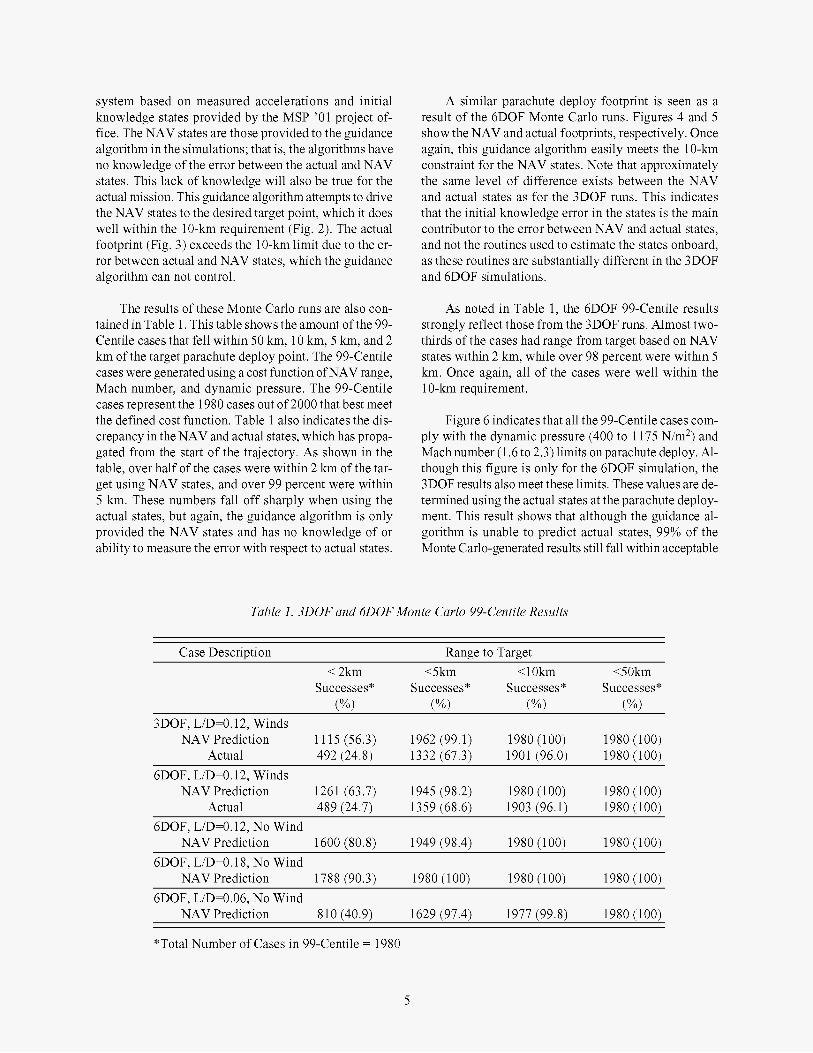
The results of these Monte Carlo runs are also con- tained in Table 1. This table shows the amount of the 99- Centile cases that fell within 50 km, 10 km, 5 km, and 2 km of the target parachute deploy point. The 99-Centile cases were generated using a cost function of NAV range, Mach number, and dynamic pressure. The 99-Centile cases represent the 1980 cases out of 2000 that best meet the defined cost function. Table 1 also indicates the dis- crepancy in the NAV and actual states, which has propa- gated from the start of the trajectory. As shown in the table, over half of the cases were within 2 km of the tar- get using NAV states, and over 99 percent were within 5 km. These numbers fall off sharply when using the actual states, but again, the guidance algorithm is only provided the NAV states and has no knowledge of or ability to measure the error with respect to actual states.

A similar parachute deploy footprint is seen as a result of the 6DOF Monte Carlo runs. Figures 4 and 5 show the NAV and actual footprints, respectively. Once again, this guidance algorithm easily meets the 1 O-km constraint for the NAV states. Note that approximately the same level of difference exists between the NAV and actual states as for the 3DOF runs. This indicates that the initial knowledge error in the states is the main contributor to the error between NAV and actual states, and not the routines used to estimate the states onboard, as these routines are substantially different in the 3DOF and 6DOF simulations.

As noted in Table 1, the 6DOF 99-Centile results strongly reflect those from the 3DOF runs. Almost two- thirds of the cases had range from target based on NAV states within 2 km, while over 98 percent were within 5 km. Once again, all of the cases were well within the 1 O-km requirement.

Figure 6 indicates that all the 99-Centile cases com- ply with the dynamic pressure (400 to 1175 N/m2) and Mach number (1.6 to 2.3) limits on parachute deploy. Al- though this figure is only for the 6DOF simulation, the 3DOF results also meet these limits. These values are de- termined using the actual states at the parachute deploy- ment. This result shows that although the guidance al- gorithm is unable to predict actual states, 99% of the Monte Carlo-generated results still fall within acceptable

Table 1. 3DOF and 6DOFMonte Carlo 99-Centile Results

Case Description Range to Target < 2km <5km <10km <50km

Successes* Successes* Successes* Successes* (%I (%I (%I (%I

3DOF, L/D=O. 12, Winds NAV Prediction 11 15 (56.3) 1962 (99.1) 1980 (100) 1980 (100)

Actual 492 (24.8) 1332 (67.3) 1901 (96.0) 1980 (100)

NAV Prediction 1261 (63.7) 1945 (98.2) 1980 (100) 1980 (100) Actual 489 (24.7) 1359 (68.6) 1903 (96.1) 1980 (100)

6DOF, L/D=0.12, Winds

6DOF, L/D=0.12, No Wind NAV Prediction 1600 (80.8) 1949 (98.4) 1980 (100) 1980 (100)

6DOF, L/D=O. 18, No Wind NAV Prediction 1788 (90.3) 1980 (100) 1980 (100) 1980 (100)

6DOF, L/D=0.06, No Wind NAV Prediction 8 10 (40.9) 1629 (97.4) 1977 (99.8) 1980 (100)

*Total Number of Cases in 99-Centile = 1980

5

NAV latitude

deg

1000

900

800

Dynamic pressure 700

Nlm2

600

500

400

NAV longitude. deg

a ~

0 0

0 0

0 0 0

~

0 0

~

~

~

B

1 8 1 8 5 190 195 2 0 0 2 0 5 210 215 2 2 0 225

Fig. 4 MSP '01 Lander parachute NAVpredicted deploy location. L /D = 0.12, 6DOF, winds,

99- Centile.

Latitude deg

Longitude. deg

Fig. 5 MSP '01 Landerparachute actual deploy location. L /D = 0.12, 6DOF, winds, 99-Centile.

Mach Number

Fig. 6 MSP '01 Lander flight conditions at parachute deploy point.

deployment conditions. Since the guidance algorithm only has knowledge of the NAV states, the remaining Lander guidance algorithm results in this paper will only present quantities derived from these estimated states.

MSP '01 Lander Trade Studies

Several trade studies were conducted to assess the robustness of this predictor-corrector guidance algorithm developed for the MSP '01 Lander missions. These stud- ies evaluated the effect of winds, lift-to-drag ratio, and parachute deploy target point on algorithm performance. The first study removed the winds provided by the MarsGRAM subroutines from the simulation. The next analysis compared the current MSP '01 Lander (with an L D = 0.12) to two other options (L/D = 0.18 and 0.06). The last study evaluated changing the target parachute deploy point to ~ 6 0 km long and TO ~ 3 0 km short of the nominal target point.

For the provided entry conditions (arrival date and states), the MarsGRAM predicted winds are predomi- nately from the southwest as the parachute deploy point is approached. This data is verified by Fig. 7 , which shows the NAV landing footprint for the 6DOF Monte Carlo without winds. By comparing Figs. 7 and 4, a tight grouping around the target point is seen. However, the target for the cases without winds had to be shifted to the southwest by ~6 km compared to the cases with winds. As seen in Table 1, the 6DOF cases without winds had slightly better performance than the cases including winds. This result indicates that the L/D = 0.12 vehicle is able to compensate for the simulated winds. The ca- veat is that this MarsGRAM model (version 3.7) does not have a wind perturbation model, thus all the entries

16 0

15 8

15 6

15 4

NAV 1 5 2

deg 1 5 0 latitude.

14 8

14 6

14 4

14 2 2630 2632 2634 2636 2638 2640 2642 2644 2646 2648 2650

NAV longitude. deg

Fig. 7 MSP '01 Lander parachute NAVpredicted deploy location. L /D = 0.12, 6DOF, no winds,

99- Centile.

6

have basically the same wind profile. This feature makes the required target offset determination simple for these Monte Carlo simulations.

12

ratio I O

08

06

Lift-to-drag

(LID)

While this paper has discussed L/D as if the Lander has a constant value during entry, this is not the case. The control system is designed to maintain the Lander at the trim angle of attack. This trim angle of attack is determined by the off-axis (lateral) center of gravity position and the aerodynamics. Since the Lander entry covers the flow regimes ranging from free molecular to continuum and hypersonic to supersonic, there is some variation in both trim angle of attack and L D . Figure 8 shows how the L/D varies with relative velocity for the three options studied. Figure 9 indicates the parachute deploy footprint for the L/D = 0.06 6DOF cases without winds and Fig. 10 has the footprint of the L/D = 0.18

< - - - _

..*' ~

- - - _ - - * - - - - - - -. LID = 0 12,s' - - --_. ~

~ /---

~

~

20 I

1 8.-.' -.-____*/-

---. -*-------_ .**-.-___

LID = 0 18

16

Velocity. mis

Fig. 8 Nominal L /D values used in MSP '01 Lander trade study.

2628 2630 2632 2634 2636 2638 2640 2642 2644 2646 2648 NAV longitude deg

Fig. 9 MSP '01 Lander parachute NAVpredicted deploy location. L /D = 0.06, 6DOF, no winds,

99-centile.

0 NAV longitude. deg

Fig. 10 MSP '01 Landerparachute NAVpredicted deploy location. L /D = 0.18, 6DOF, no winds,

99-centile.

Lander. From these figures, the 0.06 vehicle does not quite meet the 10 km requirement for 99-Centile of the cases, whereas the L D = 0.1 8 Lander is able to get all of the 99-Centile cases below 5 km. Another benefit of this increased L D of 0.1 8 is that over 90 percent of the spacecraft entries were within 2 km of the target loca- tion. For comparison, the L/D of 0.12 vehicle was able to get 8 1 percent of the entries within 2 km of the target deploy point.

A side point related to the wind/no wind trade re- ported above involves the ability of the L/D = 0.1 8 ve- hicle to handle the winds. Figure 11 shows the 6DOF footprint for this higher L/D vehicle when winds are in- cluded in the simulation and the no-wind target point is used. When compared with Fig. 4, the grouping is tighter

0 NAV longitude. deg

Fig. 11 MSP '01 Lander parachute NA Vpredicted deploy location. L /D = 0.18, 6DOF, winds,

99-centile.

7

for the higher L/D spacecraft and the target point would only need a 3 km eastward shift from the no wind target, as compared to a 6 km shift to the northeast for the L D = 0.12 vehicle.

16 25 50 km

1 4 2 5 - 1

Another analysis was conducted to assess the sensi- tivity of the algorithm to target point selection. Two new targets were selected and the only change made to the algorithm was the internal target point. One target was ~ 6 0 km down range from the original target. The other target was ~ 3 0 km up range from the original.

The 6DOF Monte Carlo results for the new target point cases without winds are shown in Figs. 12 and 13. Note that the original target point is indicated as a box

NAV longitude. deg

Fig. 12 MSP '01 Lander parachute NA Vpredicted deploy location for long-target. L /D=O.12, 6DOF,

no winds, 99-Centile.

14001 , , , , , , , , , 1 2626 2628 2630 2632 2634 2636 2638 2640 2642 2644 2646

NAV longitude deg

Fig. 13 MSP '01 Lander parachute NA Vpredicted deploy locationfor short-target. L /D=O.12, 6DOF,

no winds, 99-Centile.

in these plots. Both the short target point and long target point cases were well within the 1 O-km requirement. In fact, these figures indicate a similar result regardless of which target point is selected. This result coupled with the minimal effort to change the algorithm for these new target points indicates an algorithm fairly robust to land- ing site changes.

Aerocapture Simulation Results

Nominal Mission

Figure 14 shows angle of attack, roll angle and alti- tude versus Mars relative velocity for a nominal 3DOF aerocapture. This nominal profile requires three roll re- versals, as designed. It exits at an apoapsis of 423 km with an inclination of 93.00", and AV of 108.8 m/s re- quired for circularization into a 400 km orbit.

-5

-15

-100

-200

A l tkde ;!!/L , , , , J 1 60 40 3500 4000 4500 5000 5500 6000 6500 7000

Mars relative velocity mis

Fig. 14 Nominal MSP '01 Orbiter aerocapture using RRPC guidance algorithm.

Monte Carlo Results

Two thousand 3DOF Orbiter Monte Carlo cases using dispersions described by reference 1 were com- pleted for this guidance algorithm. Fig. 15 shows the 99-Centile inclination versus the AV required for 400 km circular orbit. This figure shows that 96.7% of the 99-Centile cases meet this criterion. Note that the dashed box indicates the inclination and AV requirements for aerocapture exit. This success level should be improved by further tuning of the algorithm. Aerocapture has been eliminated from the MSP '01 mission; thus only a small effort was devoted to guidance algorithm design for the aerocapture mission.

8

9 120- b ’ d

1 0 0

105

100 92 80 92 85 92 90 92 95 93 00 93 05

Inclination deg

Fig. 15 MSP ’01 Orbiter aerocapture exit conditions.

Conclusions

A numerical roll reversal predictor- corrector guid- ance algorithm was developed for the MSP ‘01 precision landing and aerocapture missions. These were evaluated using Monte Carlo analysis with both 3DOF and 6DOF analyses. For the precision lander, the baseline vehicle reaches the desired parachute deployment point within the acceptable range of dynamic pressures and Mach numbers. Trades were conducted that showed the impact of increased/decreased lift-to-drag ratio (L/D). Increas- ing the L/D by 50% noticeably decreased the sensitivity to winds, while decreasing the L/D to 50% of the base- line value reduced the percentage within the desired tar- get range to 94%. Thus even this large reduction in L/D still provided a large degree of precision landing capa- bility. A second trade determined the sensitivity to land- ing site selection. The trade study showed that moving the target towards either end of the landing ellipse does not significantly reduce the percentage of success.

For the Orbiter, the success of meeting the desired exit conditions after aerocapture was 96.7% of the 99- Centile cases as compared to the MSP ’01 project office requirement of 100%. The algorithm has many tunable elements that could be used to increase this success rate. Since aerocapture was dropped from the MSP ‘0 1, the major effort was placed on precision landing instead of aero capture.

References

2. Carman, G.L., and Ives, D.G. “Apollo-Derived Precision Lander Guidance,” Paper No. 98-4570, AIAA Atmospheric Flight Mechanics Conference, Boston, MA, August 1998.

3. Ro, T.U. and Queen, E.M. “Mars Aerocapture Terminal Point Guidance and Control,” Paper No. 98- 4571, AIAA Atmospheric Flight Mechanics Conference, Boston, MA, August 1998.

4. Bryant, L.E., Tigges, M., and Iacomini, C. “Ana- lytic Drag Control for Precision Landing and Aerocapture,” Paper No. 98-4572, AIAA Atmospheric Flight Mechanics Conference, Boston, MA, August 1998.

5. Tu, K.-Y., Munir, M., Mease, K., and Bayard, D. “Drag-Based Predictive Tracking Guidance for Mars Precision Landing,” Paper No. 98-4573, AIAA Atmo- spheric Flight Mechanics Conference, Boston, MA, August 1998.

6. Gamble, J. D. et. al. “Atmospheric Guidance Concepts for an Aeroassist Flight Experiment,” The Jour- nal of the Astronautical Sciences, Vol. 36, nos. 1/2 pp 45-71, Jan-Jun 1998.

7. Bourke, Roger D., Ed “Report of the Mars At- mosphere Knowledge Requirements Working Group,” May 10,1991

8. Powell, R. W. and Braun, R.D. “Six-Degree-of- Freedom Guidance and Control Analysis of Mars Aerocapture,” Journal of Spacecraft and Rockets, Vol. 30, no 5 pp 537-542, Sep-Oct 1993.

9. Willcockson, W. H. “OTV Aeroassist with Low LD,” IAF-86-115, Sep-Oct 1993.

10. Powell, R. W. “Six-Degree-of-Freedom Guid- ance and Control-Entry Analysis of the HL-20,” Jour- nal of Spacecraft and Rockets, Vol. 30, no 5 pp 537- 542, Sep-Oct 1993.

1 1. Justus, C. G. et al. “Mars Global Reference At- mospheric Model (Mars-Gram 3.34): Programmer’s Guide,” NASA TM 108509, May 1996.

1. Striepe, S. A. et al. “Development of an Atmo- spheric Guidance Algorithm Testbed for the Mars Sur- veyor 2001 Orbiter and Lander,” Paper No. 98-4569, AIAA Atmospheric Flight Mechanics Conference, Bos- ton, MA, August 1998.

9