UNIVERSITY OF SÃO PAULO

DEPARTMENT OF STRUCTURAL ENGINEERING

SÃO CARLOS SCHOOL OF ENGINEERING

ALAN BOURSCHEIDT SEITENFUSS

On the behavior of a linear elastic peridynamic material

Sobre o comportamento de um material peridinâmico elástico linear

São Carlos

2017

ALAN BOURSCHEIDT SEITENFUSS

On the behavior of a linear elastic peridynamic material

Sobre o comportamento de um material peridinâmico elástico linear

Versão corrigida

(Versão original encontra-se na unidade que aloja o Programa de Pós-graduação)

Masters dissertation submitted to the Depart-

ment of Structural Engineering, São Carlos

School of Engineering, University of São Paulo,

in partial fulllment of the requirements for the

degree of Master of Science in Civil Engineering

(Structures).

Advisor: Prof. Dr. Adair Roberto Aguiar

São Carlos

2017

ACKNOWLEDGEMENTS

I would rst like to thank my advisor Professor Adair Roberto Aguiar from the

Department of Structural Engineering at University of São Paulo, for guiding and suppor-

ting me over the past two years. I would also like to thank Professor Gianni Royer-Carfagni

from the Department of Engineering and Architecture at University of Parma in Italy, for

the great contribution to this paper. During his visit to São Carlos, the research which

resulted in the second part of this dissertation, and another work, has arisen.

My gratitude extends to CNPQ - Conselho Nacional de Desenvolvimento Cien-

tíco e Tecnológico who provided nancial support to this work, to colleagues and

employees from SET/EESC for receptiveness and attention, and to students from other

departments of EESC who have contributed, somehow, as well.

I am extremely thankful to the teachers and professors who have contributed to

my education during and before my Master's degree.

Finally, I must express my deep gratitude to my parents for providing me an

unconditional support and continuous encouragement throughout my years of study. This

accomplishment would not have been possible without them. Thank you.

ABSTRACT

SEITENFUSS, A. B. On the behavior of a linear elastic peridynamic material.2017. 69 p. Dissertation (M. Sc. in Civil Engineering (Structures)) São Carlos Schoolof Engineering , University of São Paulo, São Carlos, 2017.

The peridynamic theory is a generalization of classical continuum mechanics and takesinto account the interaction between material points separated by a nite distance withina peridynamic horizon δ. The parameter δ corresponds to a length scale and is treated asa material property related to the microstructure of the body. Since the balance of linearmomentum is written in terms of an integral equation that remains valid in the presenceof discontinuities, the peridynamic theory is suitable for studying the material behaviorin regions with singularities. The rst part of this work concerns the evaluation of theproperties of a linear elastic peridynamic material in the context of a three-dimensionalstate-based peridynamic theory, which uses the dierence displacement quotient eldin the neighborhood of a material point and considers both length and relative anglechanges. This material model is based upon a free energy function that contains fourmaterial constants, being, therefore, dierent from other peridynamic models found inthe literature, which contain only two material constants.Using convergence results of the peridynamic theory to the classical linear elasticity the-ory in the limit of small horizons and a correspondence argument between the free energyfunction and the strain energy density function from the classical theory, expressions wereobtained previously relating three peridynamic constants to the classical elastic constantsof an isotropic linear elastic material. To calculate the fourth peridynamic material cons-tant, which couples both bond length and relative angle changes, the correspondenceargument is used once again together with the strain eld of a linearly elastic beam sub-jected to pure bending. The expression for the fourth constant is obtained in terms ofthe Poisson's ratio and the shear elastic modulus of the classical theory. The validity ofthis expression is conrmed through the consideration of other experiments in mechanics,such as bending of a beam by terminal loads and anti-plane shear of a circular cylin-der. In particular, numerical results indicate that the expressions for the constants areindependent of the experiment chosen.The second part of this work concerns an investigation of the behavior of a one-dimensionallinearly elastic bar of length L in the context of the peridynamic theory; especially, nearthe ends of the bar, where it is expected that the behavior of the peridynamic bar may bevery dierent from the behavior of a classical linear elastic bar. The bar is in equilibriumwithout body force, is xed at one end, and is subjected to an imposed displacement atthe other end. The bar has micromodulus C, which is related to the Young's modulus Ein the classical theory through dierent expressions found in the literature. Dependingon the expression for C, the displacement eld may be singular near the ends, which isin contrast to the linear behavior of the displacement eld observed in classical linearelasticity. In spite of the above, it is also shown that the peridynamic displacement eldconverges to its classical counterpart as the peridynamic horizon tends to zero.

Keywords: Linear Elasticity. Nonlocal Theory. Free Energy Function. Length Scale.Finite bar. Micromodulus.

RESUMO

SEITENFUSS, A. B. Sobre o comportamento de um material peridinâmico elás-tico linear. 2017. 69 p. Dissertação (Mestrado em Engenharia Civil (Estruturas)) Escola de Engenharia de São Carlos, Universidade de São Paulo, São Carlos, 2017.

A teoria peridinâmica é uma generalização da teoria clássica da mecânica do contínuoe considera a interação de pontos materiais devido a forças que agem a uma distâncianita entre si, além da qual considera-se nula a força de interação. Por ter o balanço demomento linear formulado como uma equação integral que permanece válida na presençade descontinuidades, a teoria peridinâmica é adequada para o estudo do comportamentode materiais em regiões com singularidades. A primeira parte deste trabalho consisteno cálculo das propriedades de um material peridinâmico elástico linear no contexto deuma teoria peridinâmica de estado, linearmente elástica e tridimensional, que utiliza ocampo quociente de deslocamento relativo na vizinhança de um ponto material e leva emconta mudanças relativas angulares e de comprimento. Esse modelo utiliza uma funçãoenergia livre que apresenta quatro constantes materiais, sendo, portanto, diferente deoutros modelos peridinâmicos investigados na literatura, os quais contêm somente duasconstantes materiais.Utilizando resultados de convergência da teoria peridinâmica para a teoria de elasticidadelinear clássica no limite de pequenos horizontes e um argumento de correspondência entreas funções energia livre proposta e densidade de energia de deformação da teoria clássica,expressões para três constantes peridinâmicas foram obtidas em função das constantes deum material elástico e isotrópico da teoria clássica. O argumento de correspondêmcia,em conjunto com o campo de deformações de uma viga submetida à exão pura, é utili-zado para calcular a quarta constante peridinâmica do material, que relaciona mudançasangulares relativas e de comprimentos das ligações entre as partículas. Obtem-se umaexpressão para a quarta constante em termos do coeciente de Poisson e do módulo deelasticidade ao cisalhamento da teoria clássica. A validade dessa expressão é conrmadapor meio da consideração de outros experimentos da mecânica, tais como exão de umviga por cargas terminais e cisalhamento anti-plano de um eixo cilíndrico. Em particular,os resultados numéricos indicam que as expressões para as constantes são independentesdo experimento escolhido.A segunda parte deste trabalho consiste em uma investigação do comportamento de umabarra unidimensional linearmente elástica de comprimento L no contexto da teoria peri-dinâmica; especialmente, próximo às extremidades da barra, onde espera-se que o com-portamento da barra peridinâmica possa ser muito diferente do comportamento de umabarra elástica linear clássica. A barra está em equilíbrio e sem força de corpo, xa emuma extremidade, e sujeita a deslocamento imposto na outra extremidade. A barra pos-sui micromódulo C, o qual está relacionado ao módulo de Young E da teoria clássicapor meio de diferentes expressões encontradas na literatura. Dependendo da expressãopara C, o campo de deslocamento pode ser singular próximo às extremidades, o que con-trasta com o comportamento linear do campo de deslocamento observado na elasticidadelinear clássica. Apesar disso, é mostrado também que o campo de deslocamento peri-dinâmico converge para o campo de deslocamento da teoria clássica quando o horizonteperidinâmico tende a zero.

Palavras-chave: Elaticidade Linear. Teoria Não Local. Função Energia Livre. Escala deComprimento. Barra Finita. Micromódulo.

LIST OF FIGURES

Figure 1 Relationship among length scales. . . . . . . . . . . . . . . . . . . . 16

Figure 2 Reference and deformed congurations of a body. . . . . . . . . . . 25

Figure 3 Torsion of a nite circular shaft by a pair of couples applied to its

ends. . . . . . . . . . . . . . . . . . . . . . . . . . . . . . . . . . . . . . . . 37

Figure 4 Beam bent by terminal couples. . . . . . . . . . . . . . . . . . . . . 39

Figure 5 Beam subjected to terminal load. . . . . . . . . . . . . . . . . . . . 44

Figure 6 Numerical values of Wx0 [h] and WL

x0[h] for y0 = z0 = 0 and increa-

sing values of x0. . . . . . . . . . . . . . . . . . . . . . . . . . . . . . . . . 48

Figure 7 Shaft subjected to anti-plane shear. . . . . . . . . . . . . . . . . . . 49

Figure 8 Points considered for the anti-plane shear problem. . . . . . . . . . 51

Figure 9 Numerical values of Wx0 [h] and WL

x0[h] plotted for points on the

ξ2−axis in Fig. (8). . . . . . . . . . . . . . . . . . . . . . . . . . . . . . . . 52

Figure 10 Finite bar of length L pulled at the ends with imposed displacement

∆. . . . . . . . . . . . . . . . . . . . . . . . . . . . . . . . . . . . . . . . . 55

Figure 11 Shape of the micromodulus functions, C(ξ), for |ξ| ≤ δ. . . . . . . . 57

Figure 12 Representation of the discretized bar and boundary conditions. . . . 58

Figure 13 Displacement u(x) versus position x ∈ (0, 1) obtained from classical

linear elasticity and from peridynamics for the constant micromodulus,

N = 16000, and four values of the horizon δ. . . . . . . . . . . . . . . . . . 59

Figure 14 Displacement u(x) versus position x ∈ (0, 0.006) obtained from

classical linear elasticity and from peridynamics for δ = 1/50, N = 16000,

and four dierent micromoduli C. . . . . . . . . . . . . . . . . . . . . . . . 61

Figure 15 Ratio between relative displacement ∆u(x) and relative position

∆x versus position x ∈ (0, 0.002) obtained from peridynamics for δ = 1/50,

N = 16000, and four dierent micromoduli. . . . . . . . . . . . . . . . . . 62

Figure 16 Displacement u(x) versus position x ∈ (0, 0.003) obtained from clas-

sical linear elasticity and from peridynamics for the singular micromodulus,

δ = 1/50, and an increasing number of nodes N . . . . . . . . . . . . . . . . 62

Figure 17 Ratio between relative displacement ∆u(x) and relative position

∆x versus position x ∈ (0, 0.003) obtained for the singular micromodulus,

δ = 1/50, and increasing number of nodes N . . . . . . . . . . . . . . . . . . 63

Figure 18 Displacement u(x) versus position x ∈ (0, 1) obtained from classical

linear elasticity and from peridynamics using N = 16000 and decreasing

values of the horizon δ. . . . . . . . . . . . . . . . . . . . . . . . . . . . . . 64

Figure 19 Displacement u(x) versus position x ∈ (0, 0.006) obtained from

classical linear elasticity and from peridynamics using N = 16000 and

decreasing values of the horizon δ. . . . . . . . . . . . . . . . . . . . . . . . 64

LIST OF TABLES

Table 1 Peridynamic coecients dened in (31). . . . . . . . . . . . . . . . . 33

Table 2 Results of numerical integrations for the problem of the beam bent

by terminal loads. . . . . . . . . . . . . . . . . . . . . . . . . . . . . . . . . 47

Table 3 Terms of free energy function and strain energy density for the pro-

blem of the beam bent by terminal loads. . . . . . . . . . . . . . . . . . . . 47

Table 4 Results of numerical integrations for the anti-plane shear problem . . 51

Table 5 Terms of free energy function and strain energy density for the anti-

plane shear problem . . . . . . . . . . . . . . . . . . . . . . . . . . . . . . 52

CONTENTS

1 INTRODUCTION 15

1.1 Presentation and motivation . . . . . . . . . . . . . . . . . . . . . . . . . . 15

1.2 Objectives . . . . . . . . . . . . . . . . . . . . . . . . . . . . . . . . . . . . 17

1.3 Structure of the dissertation . . . . . . . . . . . . . . . . . . . . . . . . . . 17

2 LITERATURE REVIEW 20

2.1 Peridynamic theory . . . . . . . . . . . . . . . . . . . . . . . . . . . . . . . 20

2.2 Peridynamic bar . . . . . . . . . . . . . . . . . . . . . . . . . . . . . . . . . 22

3 THEORETICAL BASIS 25

3.1 Kinematics . . . . . . . . . . . . . . . . . . . . . . . . . . . . . . . . . . . 25

3.2 Simple peridynamic materials . . . . . . . . . . . . . . . . . . . . . . . . . 27

3.3 A linear peridynamic model . . . . . . . . . . . . . . . . . . . . . . . . . . 30

4 DETERMINATION OF FOURTH PERIDYNAMIC CONSTANT 39

4.1 Pure bending experiment . . . . . . . . . . . . . . . . . . . . . . . . . . . . 39

4.2 Determination of the constant α13 . . . . . . . . . . . . . . . . . . . . . . . 40

4.3 Bending by terminal loads experiment . . . . . . . . . . . . . . . . . . . . 44

4.4 Anti-plane shear experiment . . . . . . . . . . . . . . . . . . . . . . . . . . 48

5 PERIDYNAMIC BAR 53

5.1 1-D peridynamic model . . . . . . . . . . . . . . . . . . . . . . . . . . . . . 53

5.2 Finite bar pulled at the ends . . . . . . . . . . . . . . . . . . . . . . . . . . 54

5.3 Numerical results and Discussion . . . . . . . . . . . . . . . . . . . . . . . 56

6 CONCLUSIONS 65

REFERENCES 67

15

1 INTRODUCTION

1.1 Presentation and motivation

Fracture mechanics aims to determine whether a crack-like defect will lead a solid

to catastrophic failure under normal service loading and is a key tool in improving the

mechanical performance of materials and components. The importance of the eld is clear

when considering structures that do not admit failure.

Far from defects, stresses and deformations are smooth and can be studied in

the context of the classical theory of elasticity. This theory is local in the sense that

a material point interacts only with its immediate neighbors and that stress at a point

depends only on its own deformation. At crack tips and interfaces, displacement elds

are not smooth and classical elasticity fails to represent the behavior of materials in their

neighborhood. Many techniques have been developed to deal with cracks using classical

elasticity; however, they usually require initial knowledge of where cracks are located in the

material and how they grow. Thus, classical elasticity is not adequate when considering

fracture-related problems (GLAWS, 2014).

Peridynamics is a nonlocal theory of continuum mechanics that considers the

interaction of material points due to forces acting at a nite distance. The interaction

between particles is considered null when this distance exceeds a certain value δ called

peridynamic horizon. As the distance increases and becomes innitely large, the nonlocal

theory turns into the continuous version of the molecular dynamics model (OTERKUS,

2010). Consequently, the nonlocal theory of continuous media establishes a connection

between molecular dynamics and classical local continuum mechanics (Fig. 1).

The elastic peridynamic theory is a generalization of the classical elasticity theory

in the sense that the peridynamic operators converge to the corresponding operators of the

classical elasticity on the small horizon limit. The motivation for developing this theory

comes from the intention of modeling the behavior of solids in regions with singularities.

In contrast with the classical approach, the balance of linear momentum is formulated as

an integral equation that remains valid in the presence of discontinuities, such as in the

case of Grith cracks (SILLING et al., 2007).

The damage is incorporated at the level of interaction between two particles and,

thus, the location of the crack and the fracture occur as a consequence of the equation of

16

Figure 1: Relationship among length scales.

Source: Oterkus (2010).

motion and the constitutive model (SILLING et al., 2007). Cracks start and propagate

naturally based on deformation of the material, as opposed to techniques based on classical

continuum mechanics, where it is necessary to know the initial position of the crack to

predict its propagation.

To achieve the goal of predicting crack formation and propagation, a simple, con-

sistent, and eective material model is needed. The model should be simple enough to

be amenable to analysis, veriable experimentally, and easily implemented in computati-

onal codes. It should also be consistent with classical theories away from singular points,

such as crack tips and points on interfaces between two dierent materials, and eective

in modeling propagation of cracks and phase interfaces. This work aims at contributing

to both the development of the linear peridynamic theory and the modeling of classical

problems in mechanics, such as torsion of cylindrical bars, bending of cylindrical beams,

and anti-plane shear of hollow cylinders, using a peridynamic model proposed by our

group. With a strong theoretical basis, we will extend the results of this investigation

to the analysis of fracture mechanics problems, in which formation and propagation of

cracks will be the major concern, and phase transitions problems, in which attention will

be focused to the formation and propagation of phase interfaces in nonlinear elastic solids

with non-convex energy densities.

In this paper, we use a correspondence argument proposed in earlier work together

with the non-homogenous deformation of a beam bent by terminal couples to obtain an

expression for a fourth peridynamic constant in a material model also proposed earlier

in terms of the classical elasticity constants. To verify the validity of the expressions

obtained for all peridynamic constants, we consider dierent experiments in mechanics

17

and verify that the correspondence argument is nearly satised in all cases. In the second

part of this work , we investigate linear elastic peridynamic bars of nite length being

pulled at the ends. The bars have dierent expressions for material micromoduli C,

which are related to the Young's modulus E in the classical theory. Depending on the

micromodulus, numerical results indicate that the displacement eld is discontinuous, or,

has unbounded derivatives at the ends. Either behavior is in contrast to the homogeneous

deformation of the bar predicted by the classical linear theory. Nevertheless, in all cases,

the numerical results converge to results obtained from the classical linear theory as a

certain scale parameter, called horizon, tends to zero.

1.2 Objectives

The general objective of this work is to contribute, through a theoretical and

numerical study, to the development of the peridynamic model proposed by Aguiar e

Fosdick (2014).

The specic objectives are listed below.

- To determine the peridynamic constant (α13) of the model proposed by Aguiar

e Fosdick (2014), relating it to the elastic constants from classical theory;

- To verify the validity of the expressions of the peridynamic constants that appear

in this author's model by considering classical problems in mechanics.

- To formulate and to solve one-dimensional peridynamic bar problems and in-

vestigate nonlocal eects; especially, near the bar ends.

- To analyze the results of the peridynamic bar problem and the eect of the

micromodulus choice.

1.3 Structure of the dissertation

In Section 2 we review the literature on peridynamics by discussing some re-

cent developments of the theory, applications of the theory on practical problems, and

investigations of one-dimensional peridynamic bar problems. In Chapter 3 we recall the

three-dimensional state-based linearly elastic peridynamic theory developed by Aguiar e

Fosdick (2014). We start by introducing some kinematical concepts on innitesimal mea-

sures of angular distortion and length changes between material points in Section 3.1. In

Section 3.2 we present the force response function state of a simple material and restrict

18

its form based on the free energy function proposed by Aguiar e Fosdick (2014) which is

expressed in terms of the innitesimal measures of deformation. Expressions for the strain

energy function and the linearized force vector state proposed by Silling et al. (2007) are

presented in Section 3.3. It then is observed that these expressions correspond to par-

ticular cases of the expressions proposed by Aguiar e Fosdick (2014). A correspondence

argument is introduced and used in the determination of three peridynamic constants

that appear in the expressions of these authors.

In Section 4.1 we present the experiment of a cylindrical linear elastic beam bent

by terminal couples and the corresponding displacement eld in classical theory. The

use of this experiment along with the correspondence argument mentioned above allows

to obtain a closed-form expression for a fourth peridynamic constant, that appears in

the peridynamic model proposed by Aguiar and Fosdick (2014), in Section 4.2. The

determination of this constant is one of the main goals of this work. To obtain this

constant, we have used a xed point at the origin of the coordinate system. We then show

that the same expression is found if any other point inside the beam is used. In Section 4.3

we consider the experiment of an elastic beam bent by terminal loads and use it to verify

the validity of the closed expressions of the four peridynamic constants that appear in

the model proposed by Aguiar and Fosdick (2014). For this, we evaluate numerically the

free energy function and the classical strain energy density function for this experiment

and use these calculations to verify that the correspondence argument mentioned above is

approximately satised for given values of mechanical and geometrical properties and at

several points inside the beam. A similar verication is conducted in Section 4.4, where

we consider the experiment of a cylindrical shaft subjected to anti-plane shear.

The other main goal of this work is to investigate the behavior of the displacement

eld of a one-dimensional linearly elastic bar of length L near its ends in the context of the

peridynamic theory. The one-dimensional peridynamic governing equation is presented

in Section 5.1. In Section 5.2 we formulate the problem of an elastic peridynamic bar in

equilibrium without body force being subjected to imposed displacements at its ends. The

problem is then recast in terms of an inhomogeneous Fredholm equation, which assumes

a simplied form in the case of a constant micromodulus. In Section 5.3 we present the

numerical scheme used to obtain approximate solutions for dierent expressions of the

micromodulus found in the literature. These solutions are highly nonlinear in a boundary

19

layer near the ends and may be either discontinuous or singular at these ends. We then

concentrate our attention on a particular micromodulus that yields a singular behavior of

the solution near the ends. Using this micromodulus, we study both convergence of the

proposed numerical scheme and convergence of the nonlocal model to the classical linear

elastic model as the horizon δ tends to zero. In Chapter 6 we present some concluding

remarks.

20

2 LITERATURE REVIEW

The solutions of problems in fracture mechanics within the classical continuum

theory yield innite stresses at crack tips, as was shown in Grith (1921)'s pioneering

work. In this context, the appearance and growth of cracks are treated separately by

introducing external criteria, such as the critical rate of deformation energy release, which

is not part of the governing equations of classical continuum mechanics. In addition, a

criterion is also necessary for the determination of the direction of propagation of the

cracks. The understanding and prediction of the failure processes of a material are more

complex due to the presence of mechanisms associated with grain boundary, microcracks,

anisotropy, etc, which interfere with the material response in a certain length scale. Since

in the local continuous theory a material point is inuenced only by the immediately

neighboring points, there is no internal length scale that allows to consider the eect of

these damage mechanisms (MADENCI; OTERKUS, 2014).

In order to account for long-range eects, the theory of the nonlocal continuum

was introduced (ERINGEN; EDELEN, 1972; KRONER, 1967). In this theory, the stress

eld at the crack tip is limited (ERINGEN; KIM, 1974), rather than the unlimited stress

predicted in the classical theory. In spite of obtaining nite stresses at crack tips, this

theory still presents discontinuities in the derivative of the displacement eld due to the

presence of the cracks. A dierent nonlocal theory proposed by Kunin (1982) circumvented

this diculty by using displacement elds rather than their derivatives.

2.1 Peridynamic theory

Silling (2000) proposes the peridynamic formulation as a new form of the basic

equations of the continuum mechanics intending to model discontinuities formed in the

material. To describe the interaction between material points, the author supposes the

existence of a force function between two particles that depends only on the relative

displacement and the relative positions between the particles. Thus, this model, which

is called bond-based model, is restricted to relatively simple interactions between two

points.

Silling et al. (2007) develop a generalized form of this model, called the state-

based model, which allows the response of a material at a point to depend collectively

21

on the deformation of all bonds connected to the point. In this work, the authors obtain

an energy function for the simple elastic peridynamic material that, as in the classical

elasticity theory for isotropic materials, depends only upon two material peridynamic

constants. The constitutive laws of this model are signicantly more general than the

constitutive laws of the binding model. This allows more complex material responses to

be modeled numerically at the cost of higher computational cost.

Silling (2010) uses the state-based theory to study the behavior of a peridynamic

material by applying a small deformation superposed on a large one and introduced the

concept of modulus state. The modulus state expresses the material properties of the

linearized response and it is obtained from the second Fréchet derivative of the free energy

function for an elastic material. In the case that the deformation of a body is smooth

and considering that the behavior of a sequence of peridynamic elastic materials does not

change in the limit of vanishing distances between material points, Silling (2010) obtains

relations between the modulus state and the fourth-order elasticity tensor in classical

continuum theory.

Many works have used successfully peridynamics to predict damage in dierent

problems. Examples include the investigations of Gerstle, Sau e Silling (2005) on plain

reinforced concrete structures under quasi-static loading and Askari, Xu e Silling (2006)

on a composite laminate under low-velocity impact loading. Warren et al. (2009) de-

monstrate the capability of a nonordinary state-based model for capturing failure based

on either the critical equivalent strain or the averaged value of the volumetric strain.

The authors capture the failure behavior of the solid using both isotropic notched and

un-notched bar subjected to quasi-static loadings. Oterkus, Barut e Madenci (2010) pre-

sent an approach based on the merger of classical continuum theory and peridynamic

theory to capture failure modes in bolted composite lap joints. The simulations capture

the dominant failure modes in the region where the bolt is in contact with the lami-

nate, consistently with common failure modes around the bolt hole observed in previous

experimental investigations.

Hu, Ha e Bobaru (2012) use peridynamics to analyse dynamic eects of loading

on the damage behavior of unidirectional ber-reinforced composites. The model cap-

tures signicant dierences in the crack propagation behavior when dynamic loadings of

dierent intensities are applied. Hu et al. (2013) simulate fracture patterns caused by

22

the impact of a spherical projectile on a thin glass plate with a thin polycarbonate bac-

king plate using a peridynamic simplied model. The main fracture patterns observed

experimentally are captured by the peridynamic model for the three dierent projectile

velocities tested

Littlewood, Mish e Pierson (2012) apply peridynamics in combination with modal

analysis in the prediction of characteristic frequency shifts that occur during the damage

evolution process and demonstrate this application on the benchmark problem of a sim-

ply supported beam. Oterkus, Guven e Madenci (2012) consider a reinforced concrete

panel subjected to multiple load paths to predict residual strength of impact damaged

in building components. To demonstrate the eectiveness of the peridynamic theory for

assessment of residual strength of structures, they take a panel with steel reinforcements

under impact of an rigid penetrator and another subjected to compression. Zhou, Gu

e Wang (2015) and Ha, Lee e Hong (2015) simulate successfully the crack propagation

process in rock-like materials subjected to uni-axial tensile and compression loads, respec-

tively. Diyaroglu et al. (2016) demonstrate the applicability of peridynamics to accurately

predict nonlinear transient deformation and damage behavior of composites under shock

or blast types of loadings due to explosions.

Aguiar e Fosdick (2014) present a three-dimensional state-based linearly elastic

peridynamic theory using the relative displacement eld between particles. The authors

propose a free energy function that depends on deformation measures that are analogous

to the measures of strain in classical linear elasticity theory and contains four elastic

peridynamic constants. Using vanishing sequences of the horizon δ, the authors nd two

relations between three peridynamic constants and the two Lamé constants of classical

linear elasticity.

In order to obtain a third relation, Aguiar (2016) introduces a correspondence

argument between the free energy peridynamic function and a weighted average of the

energy density function of the classical theory. This argument provides the two relations

mentioned above in the case of homogenous deformations, being, therefore, compatible

with the theory presented by Aguiar e Fosdick (2014). Aguiar (2016) uses this argument

along with the non-homogenous deformation of a circular shaft under uniform torsion to

obtain the third relation. This relation along with those two relations mentioned above

allow evaluating three of the four peridynamic constants.

23

Recall from the exposition in previous sections that a goal of this work is to use

the correspondence argument to determine the fourth peridynamic constant and to verify

the validity of all formulae found thus far for these constants.

2.2 Peridynamic bar

The eects of long-range forces in the peridynamic theory have motivated the

study of one-dimensional bars of innite length made of linearly elastic peridynamic ma-

terials. The corresponding problems are formulated in terms of linear Fredholm integral

equations, which are solved by Fourier transform techniques; thus, providing Green's func-

tions for general loading applications. These solutions exhibit features that are not found

in their counterparts in the classical linear elasticity theory and are shown to converge to

these classical solutions in the limit of short-range forces.

One feature of interest was observed by Silling et al. (2007) in the analysis of a bar

with constant micromodulus in (−δ, δ), where δ is the horizon, under a single concentrated

load. Even though the displacement eld obtained from the solution of the corresponding

static problem in the classical linear theory is bounded and continuous at all points of the

bar, its counterpart in the linear peridynamic theory is unbounded at the point where the

force is applied.

Some additional works on one-dimensional bars of innite length made of linearly

elastic peridynamic materials include the investigation of Weckner e Abeyaratne (2005) on

the one-dimensional dynamic response of an innite bar composed of a linear microelastic

material. For a Riemann-like problem corresponding to a constant initial displacement

eld and a piecewise constant initial velocity eld the authors nd peridynamic solution

involving a jump discontinuity for all times after the initial continuous displacement eld.

Dayal e Bhattacharya (2006) apply the peridynamic formulation of the motion of phase

boundaries in one dimension to study the kinetics of phase transformations in solids.

They examine nucleation by viewing it as a dynamic instability and propose a nucleation

criterion, in which nucleation occurs when the defect size reaches a critical value

Mikata (2012) develops a systematic analytical treatment of peristatic and pe-

ridynamic problems for a one-dimensional innite rod. In order to obtain the exact

analytical solutions for the problems the author transforms divergent integrals obtained

by Fourier transform into singular solutions plus convergent integrals. Wang, Xu e Wang

24

(2017a, 2017b) derive the static and dynamic Green's functions for one-, two- and three-

dimensional innite domains considering peridynamics and making use of both Fourier

transforms and Laplace transforms. Bobaru et al. (2009) investigate adaptive renement

and convergence in one-dimensional peridynamics. They use adaptive and uniform re-

nement and dierent continuous and discontinuous micromoduli for static and dynamic

elasticity problems in one dimension. They nd that using discontinuous micromodulus

functions reduces the quadratic rate of convergence to linear result and that solutions

obtained on uniform grids were not sensitive to the micromodulus shape, in the limit of

horizon going to zero.

In this work we investigate the behavior of linearly elastic peridynamic bars of

nite lengths subjected to displacement conditions at their ends. The bars have distinct

micromoduli that can be found in the literature. The main ndings of this investigation,

which shed new light on the behavior of nite peridynamic bars, consist of a highly

nonlinear behavior of the bars near their ends. This is in contrast to what is observed in

classical linear elasticity, where the deformation is homogeneous.

25

3 THEORETICAL BASIS

3.1 Kinematics

The three-dimensional state-based linearly elastic peridynamic theory presented

in this chapter was developed by Aguiar and Fosdick (2014) and is also presented in

Aguiar (2015). The derivations shown in Section 3.3 after (38) were originally presented

in Aguiar (2016).

Let B ∈ E3 be the undistorted reference conguration of an elastic body and let

y := χχχ(x, t) be the position of the particle x ∈ B at time t ≥ 0. Here, a neighborhood

of any point x0 where we consider the collective deformation of the material is a sphere

of radius δ centered at x0, which we denote by N δ(x0) ⊂ B. The vector ξξξ := x − x0 is

called a bond from x to x0, where x ∈ Nδ, as illustrated in Fig. 2. The set Hδ(x0) is the

collection of all bonds to x0.

Figure 2: Reference and deformed congurations of a body.

Source: Aguiar e Fosdick (2014).

A peridynamic state at (x0, t) of order m is a function A(x0, t)〈·〉 : Hδ(x0)→ Lm,

where Lm is the set of all tensors of orderm. Thus, the image of a bond ξ ∈ Hδ(x0) for the

stateA(x0, t)〈·〉 is the tensor of orderm,A(x0, t)〈ξξξ〉. We denote byAm the set of all states

at (x0, t) of order m. Similarly, we introduce the denition of a double state at (x0, t)

of order p, D(x0, t)〈·, ·〉 : Hδ(x0) × Hδ(x0) → Lp. The dependency between two states

A(x0, t)〈·〉 : Hδ(x0) → Lm and u(x0, t)〈·〉 : Hδ(x0) → Lp is denoted by A(x0, t)〈ξξξ〉 =

A(x0, t)[u]〈ξξξ〉. For notational convenience, we shall not exhibit the dependence on the

26

time variable t and, when the meaning is clear, may also omit the dependence on the

particle x0.

The dierence deformation state χχχ ∈ A1 at x0 ∈ B is dened through

χχχ〈ξξξ〉 := (χχχ(x)−χχχ(x0)) |x=x0+ξξξ .

With u ∈ A1 being the dierence displacement state and x ∈ A1 the reference position

vector state at x0 ∈ B, we may write χχχ = u + x. The dierence deformation and

displacement quotient states at x0 ∈ B are then dened by

f :=χχχ

|x|= h + e, h :=

u

|x|, (1)

respectivelly, where

e :=x

|x|, (2)

and |A| is the magnitude state of A, dened through

|A| 〈ξξξ〉 :=√A〈ξξξ〉 ·A〈ξξξ〉. (3)

We select two bonds ξξξ = x− x0 e ηηη = y − y0 in Hδ, with α := α〈ξξξ,ηηη〉 being the

smallest included angle. We then have that cosα = e〈ξξξ〉 · e〈ηηη〉. After deformation, the

angle will change to β := β〈ξξξ,ηηη〉, which is determined by

cosβ =χχχ〈ξξξ〉|χχχ〈ξξξ〉|

·χχχ〈ηηη〉|χχχ〈ηηη〉|

= (h〈ξξξ〉+ e〈ξξξ〉) · (h〈ηηη〉+ e〈ηηη〉)( 1

|f〈ξξξ〉|1

|f〈ηηη〉|). (4)

When the deformation of the body is small, we suppose that there is an ε, |ε| < 1,

such that, at x0 ∈ B, h〈ξξξ〉 ≡ u〈ξξξ〉/|ξξξ| = O(ε), |ξξξ| < δ. Using (1) and (3), we get

|f〈ξξξ〉| ≡|χχχ〈ξξξ〉||ξξξ|

= 1 + e〈ξξξ〉 · h〈ξξξ〉+ O(ε2). (5)

The strain of a bond ξξξ at x0 is dened as the change of length of ξξξ per unit of

length ξξξ as the result of a deformation, i.e., e〈ξξξ〉 := (|χχχ| − |ξξξ|)/|ξξξ|. Thus, the innitesimal

normal strain state ε〈·〉 : Hδ → R at x0 is given by the second term on the right-hand

27

side of (5), viz.,

ε〈ξξξ〉 := ε[h]〈ξξξ〉 ≡ e〈ξξξ〉 · h〈ξξξ〉. (6)

From (6) we see that ε[·]〈ξξξ〉 : A1 → R is a linear function.

Using (4) and (5), we get

cosβ = cosα + (e〈ξξξ〉 − e〈ηηη〉cosα) · h〈ηηη〉+ (e〈ηηη〉 − e〈ξξξ〉cosα) · h〈ξξξ〉+ O(ε2).

Using the trigonometric identities sin(α−β) = sinα cosβ−cosα sinβ and sinβ =√1− cos2β and linearizing the dierence between angles α and β, we get

α− β =1

sinα[(e〈ξξξ〉 − e〈ηηη〉cosα) · h〈ηηη〉+ (e〈ηηη〉 − e〈ξξξ〉cosα) · h〈ξξξ〉] + O(ε2).

Next, we dene the innitesimal shear strain state γ〈·, ·〉 : Hδ(x0)×Hδ(x0)→ R

through the expression

γ〈ξξξ,ηηη〉 := γ[h]〈ξξξ,ηηη〉 ≡ 1

2(e〈ξξξ,ηηη〉 · h〈ξξξ〉+ e〈ηηη, ξξξ〉 · h〈ηηη〉), |ξξξ| < δ, |ηηη| < δ, (7)

where we have used the notation

e〈ξξξ,ηηη〉 :=(111− e〈ξξξ〉 ⊗ e〈ξξξ〉)e〈ηηη〉

sinα=

e〈ηηη〉 − e〈ξξξ〉cosαsinα

, (8)

in which 111 is the identity tensor in L2 and α is the smallest included angle between ξξξ and

ηηη. From (7) and (8) we see that γ[·]〈ξξξ,ηηη〉 : A1 → R is also a linear function.

3.2 Simple peridynamic materials

In the state-based theory introduced by Silling et al. (2007), the equation of

motion is given by

ρ(x0)u(x0) =

∫Nδ

T(x0)〈x− x0〉 −T(x)〈x0 − x〉dvx + b(x0), (9)

where ρ is the mass density in the reference conguration, u is the displacement eld,

b is a prescribed body force density eld, both evaluated at x0, and both T(x0)〈·〉 and

T(x)〈·〉 are force vector states evaluated on bonds, respectively, at x0 and x.

28

We say that a peridynamic material is simple if, for any x0 ∈ B, there is a force

response function state Tx0 [·]〈ξξξ〉 : A1 → L1, such that

T = Tx0 [f ].

Using both frame indierence and material symmetry conditions, Aguiar e Fos-

dick (2014) restrict the general form of the force response function. For an isotropic and

simple material, the function satises the relation

QT Tx0 [(Qf) qT ]〈Qξξξ〉 = Tx0 [f ]〈ξξξ〉, ξξξ ∈ Hδ, ∀Q ∈ Orth+,

where qT := QTx and Orth+ is the set of orthogonal positive transformations.

The superposition of a small dierence displacement quotient state h onto a

dierence deformation quotient state f yields a general expression for the response function

of a simple isotropic material in the vicinity of the reference conguration of a peridynamic

body, which is given by

(δf Tx0 [e] • h)〈ξξξ〉 = (QT δf Tx0 [e] • ((Qh) qT ))〈Qξξξ〉, (10)

where e is given by (2) and δf is the Fréchet derivative of a vector state.

The linearized force response function state Lx0 [h] is dened by

Lx0 [h] := Tx0 [f ] + δf Tx0 [f ] • h. (11)

Aguiar e Fosdick (2014) introduce the function Ψ[·] : A1 → R that represents the free

energy at x0 due to the dierence deformation quotient state f at x0 and show that, for

an elastic simple material,

Tx0 [f ] =δf Ψx0 [f ]

|x|. (12)

With (12), we can write (11) as

Lx0 [h] =δf Ψx0 [f ]

|x|+

(δ2f Ψx0 [f ]) • h|x|

. (13)

Now, we consider the identity map χχχ = x, so that f = e and dene the free energy

29

function Wx0 by

Wx0 [h] :=1

2(δ2

f Ψx0 [e] • h) • h, (14)

so that

δhWx0 [h] := δ2f Ψx0 [e] • h. (15)

In the case of null residual force state the rst term on the right-hand side of (13)

is the null tensor, so from (15) and (13) we obtain

Lx0 [h] =δhWx0 [h]

|x|. (16)

Aguiar e Fosdick (2014) propose a free energy function for a simple elastic material

that satises the invariance condition (10). The function presented below has a quadratic

form and uses the innitesimal strains ε[h] and γ[h] dened in (6) and (7), respectively.

Wx0 [h] =

∫Nδ

∫Nδ

ω(|ξξξ|, |ηηη|)α11

2(ε[h]〈ξξξ〉)2 +

α22

2(ε[h]〈ηηη〉)2

+ α12ε[h]〈ξξξ〉ε[h]〈ηηη〉+α33

2(γ[h]〈ξξξ,ηηη〉)2 + α13γ[h]〈ξξξ,ηηη〉ε[h]〈ξξξ〉

+ α23γ[h]〈ξξξ,ηηη〉ε[h]〈ηηη〉dvηdvξ,

(17)

where ω(·, ·) is a given weighting function and αij, i, j =1, 2, 3, are elastic peridynamic

constants. Assuming that the weighting function ω(·, ·) is symmetric, i.e., ω(|ξξξ|, |ηηη|) =

ω(|ηηη|, |ξξξ|), we can write (17) as

Wx0 [h] =

∫Nδ

∫Nδ

ω(|ξξξ|, |ηηη|) α11

2(ε[h]〈ξξξ〉)2 + α12ε[h]〈ξξξ〉ε[h]〈ηηη〉

+α33

2(γ[h]〈ξξξ,ηηη〉)2 + α13γ[h]〈ξξξ,ηηη〉ε[h]〈ξξξ〉dvηdvξ,

(18)

where we have dened α11 := α11 + α22 and α13 := α13 + α23.

Replacing (6) and (7) into (18), the free energy function can be rewritten as

Wx0 [h] =

∫Nδ

h〈ξξξ〉 ·∫Nδ

ω(|ξξξ|, |ηηη|) α11

2(e〈ξξξ〉 ⊗ e〈ξξξ〉)h〈ξξξ〉+ α12(e〈ξξξ〉 ⊗ e〈ηηη〉)h〈ηηη〉

+α33

4[(e〈ξξξ,ηηη〉 ⊗ e〈ξξξ,ηηη〉)h〈ξξξ〉+ (e〈ηηη, ξξξ〉 ⊗ e〈ηηη, ξξξ〉)h〈ηηη〉]

+α13

2[(e〈ξξξ,ηηη〉 ⊗ e〈ξξξ〉)h〈ξξξ〉+ (e〈ξξξ,ηηη〉 ⊗ e〈ηηη〉)h〈ηηη〉]dvηdvξ.

(19)

30

Using (19), we get

δhWx0 [h]〈ξξξ〉 =

∫Nδ

ω(|ξξξ|, |ηηη|)α11(e〈ξξξ〉 ⊗ e〈ξξξ〉)h〈ξξξ〉+ α12(e〈ξξξ〉 ⊗ e〈ηηη〉)h〈ηηη〉

+α33

2[(e〈ξξξ,ηηη〉 ⊗ e〈ξξξ,ηηη〉)h〈ξξξ〉+ (e〈ηηη, ξξξ〉 ⊗ e〈ηηη, ξξξ〉)h〈ηηη〉]

+α13

2[(e〈ξξξ〉 ⊗ e〈ξξξ,ηηη〉+ e〈ξξξ,ηηη〉 ⊗ e〈ξξξ〉)h〈ξξξ〉

+ (e〈ηηη〉 ⊗ e〈ηηη, ξξξ〉+ e〈ξξξ,ηηη〉 ⊗ e〈ηηη〉)h〈ηηη〉]dvηdvξ.

3.3 A linear peridynamic model

By assuming smooth deformation. Lehoucq e Silling (2008) have shown that the

peridynamic equation of motion is equivalent to the partial dierential equation

ρ(x)u(x) = divS(x) + b(x), ∀x ∈ B, (20)

which similar to the equation of motion of the classical theory. In the equation (20), S is

the peridynamic stress tensor, given by

S(x) =

∫N1

∫ δ

0

∫ δ

0

(y + z)2T[x− zm]〈(y + z)m〉 ⊗m d z d y dΩm,

where ⊗ denotes the dyadic product of two vectors, T is the force vector state, N1 is the

unit sphere and Ωm is a dierential solid angle on N1 in the direction of any unit vector

m.

Let Ψx0 be the free energy function at an arbitrary point x0 ∈ B. Consider

also a family of peridynamic simple elastic materials parameterized by a variable horizon

δs = sδ, where δ is held xed, and given by

Ψsx0

[f ] := Ψx0 [Esf ]. (21)

In (21), Es is an enlarged dierence deformation quotient state dened by

Es[f ]〈ξξξ〉 = f〈sξξξ〉, ∀ξξξ ∈ Hδ, ∀f ∈ A1.

31

The peridynamic stress tensor associated with Ψsx0

is given by

Ss(x0) =

∫N1

∫ δ

0

∫ δ

0

(y + z)2Tx0−szm[Es[f(x0 − szm)]]〈(y + z)m〉 ⊗m d z d y dΩm.

Assuming that the motion χχχ is twice continuously dierentiable and that Tx0

is continuously dierentiable with respect to χχχ and to the position x, Silling e Lehoucq

(2008) have shown that

lims→0

Ss = P em B,

where P is the PiolaKirchho stress eld of the classical theory, which is related to the

response function Tx0 of a linear peridynamic material by

P(x0) =

∫Nδ

Tx0 [F(x0)e]〈ξξξ〉 ⊗ ξξξdvξ, (22)

and F(x0) is the deformation gradient tensor at x0 given by

F(x) =∂χχχ(x)

∂x= 111 + H(x), H(x) :=

∂u(x)

∂x.

Assuming that the displacement gradient H0 := H(x0) is small, the expression

(22) can be approximated by

PL(x0) =

∫Nδ

δhWx0 [H0e]〈ξξξ〉 ⊗ e〈ξξξ〉dvξ. (23)

Taking the inner product between H0 and PL(x0) in (23), we obtain

H0 ·PL(x0) =

∫Nδ

tr[δhWx0 [H0e]〈ξξξ〉 ⊗ (H0e〈ξξξ〉)

]dvξ = (H0e) • δhWx0 [H0e].

Using (14) and (15) in the above expression, we get

1

2H0 ·PL(x0) = Wx0 [H0e]. (24)

It then follows from the above result that, in the limit of small horizon, both the

classical continuum theory and the peridynamic theory yield the same energy at a point

x0 in the vicinity of the reference conguration.

The Generalized Hooke's Law in classical linear elasticity relates the tensorPL(x0)

32

to the innitesimal displacement gradient tensor H0 through PL(x0) = Cx0H0, where Cx0

is the elasticity tensor at x0. Substituting this relation into (24), we get

1

2H0 · (Cx0H0) = Wx0 [H0e]. (25)

For the linearized simple elastic material given by the free energy function (19),

we have that

1

2H0 · (Cx0H0) =

1

2H0 ·

∫Nδ

∫Nδ

ω(|ξξξ|, |ηηη|)[α11 e〈ξξξ〉 ⊗ e〈ξξξ〉 ⊗ e〈ξξξ〉 ⊗ e〈ξξξ〉

+ 2α12 e〈ξξξ〉 ⊗ e〈ξξξ〉 ⊗ e〈ηηη〉 ⊗ e〈ηηη〉

+α33

2e〈ξξξ,ηηη〉 ⊗ e〈ξξξ〉 ⊗ (e〈ξξξ,ηηη〉 ⊗ e〈ξξξ〉+ e〈ηηη, ξξξ〉 ⊗ e〈ηηη〉)

+ α13(e〈ξξξ,ηηη〉 ⊗ e〈ξξξ〉+ e〈ηηη, ξξξ〉 ⊗ e〈ηηη〉)⊗ e〈ξξξ〉 ⊗ e〈ξξξ〉]dvηdvξH0.

(26)

Aguiar e Fosdick (2014) show that all the integral terms that multiply α13 in the

expression (26) vanish. We then conclude that the terms multiplied by α13 do not contri-

bute to the free energy Wx0 [H0e] of a peridynamic body at x0 in the limit of vanishing

horizon.

Being ξi, ηi the components of x〈ξξξ〉 ≡ ξξξ and x〈ηηη〉 ≡ ηηη, respectively, and e1, e2, e3

a xed basis, it follows from (2) that

e〈ξξξ〉 :=ξi|ξξξ|

ei, e〈ηηη〉 :=ηi|ηηη|

ei. (27)

Replacing (27) into (8) yields

e〈ξξξ,ηηη〉 :=1

sinα

(ηi|ηηη|− cosα ξi

|ξξξ|

)ei, e〈ηηη, ξξξ〉 :=

1

sinα

(ξi|ξξξ|− cosα ηi

|ηηη|

)ei. (28)

With Cijkl, i,j,k,l=1,2,3, being the classical elastic constants and Hij the compo-

nents of H0, we write1

2H0 · (Cx0H0) =

1

2HijCijklHkl. (29)

Substituting (27), (28), and (29) into the expression (26), we get

Cijkl = α11C11ijkl +

α33

2C33ijkl + 2α12C

12ijkl, (30)

33

where

C11ijkl ≡

∫Nδ

∫Nδ

ω(|ξξξ|, |ηηη|)dvηξiξjξkξl|ξξξ|4

dvξ,

C33ijkl ≡

∫Nδ

∫Nδ

ω(|ξξξ|, |ηηη|)sin2α

(ηi|ηηη|− cosα ξi

|ξξξ|

)ξj|ξξξ|[(

ηk|ηηη|− cosα ξk

|ξξξ|

)ξl|ξξξ|

+

(ξk|ξξξ|− cosα ηk

|ηηη|

)ηl|ηηη|

]dvηdvξ,

C12ijkl ≡

∫Nδ

∫Nδ

ω(|ξξξ|, |ηηη|) ξiξjξkξl(|ξξξ||ηηη|)2

dvηdvξ.

(31)

The Cartesian coordinates ξi, ηi are given in terms of the spherical coordinates

(ρ, θ, φ), (ρ, θ, φ) through

(ξ1, ξ2, ξ3) = ρ(cosθ sinφ, sinθ sinφ, cosφ),

(η1, η2, η3) = ρ(cosθ sinφ, sinθ sinφ, cosφ).(32)

Substituting (32) into (31) and taking the limits of integration on Nδ as

ρ ∈ (0, δ), φ ∈ (0, π) and θ ∈ (0, 2π), (33)

we have the values presented in Tab. 1, in which ωδ ≡ π2∫ δ

0

∫ δ0ω(ρ, ρ)ρ2ρ2dρdρ.

Table 1: Peridynamic coecients dened in (31).

(i,j,k,l) C11ijkl/ωδ C33

ijkl/ωδ C12ijkl/ωδ

(1, 1, 1, 1) 16/5 1.4221≈64/45 16/9

(2, 2, 2, 2) 16/5 1.4221≈64/45 16/9

(3, 3, 3, 3) 16/5 1.4221≈64/45 16/9

(1, 1, 2, 2) 16/5 -0.7111≈-32/45 16/9

(1, 1, 3, 3) 16/5 -0.7111≈-32/45 16/9

(2, 2, 3, 3) 16/5 -0.7111≈-32/45 16/9

(2, 3, 2, 3) 16/5 1.0667≈16/15 0

(1, 3, 1, 3) 16/5 1.0667≈16/15 0

(1, 2, 1, 2) 16/5 1.0667≈16/15 0

The matrices with components C11ijkl e C

12ijkl have minor and major symmetries. The

symmetry for the coecients C33ijkl is given by C33

ijkl = C33jikl = C33

ijlk = C33klij. The coecients

34

not shown in the table and that do not satisfy the cited simmetries are zero.

Substitution of the values of Tab. 1 into (30) yields a system of equations for the

calculations of the constants α11, α12 e α33 in terms of the elastic constants Cijkl. This

system has no solution unless the following relations are satised.

Cii23 = Cii13 = Cii12 = 0,

C2313 = C1312 = C2312 = 0,

C2222 = C1111 = C3333,

C1133 = C2233 = C1122,

C2323 = C1313 = C1212 = (C1111 − C1122)/2.

(34)

Clearly the values of Tab. 1 substituted in (30) yield elastic constants that satisfy the

relations in (34). Also, these relations imply that the classical elastic material must be

istropic. Using (30), (34) and Tab. 1, we get the relations

2α11 + α33 =15(C1111 − C1122)

16ωδ, α11 + 2α12 =

3(C1111 + 2C1122)

16ωδ. (35)

Writing the constants of the isotropic elastic material in terms of Young's modulus

(E) and Poisson's ratio (ν), we have that

C1111 =E(1− ν)

(1 + ν)(1− 2ν), C1122 =

νE

(1 + ν)(1− 2ν). (36)

Substitution of (36) into (35), yields

2α11 + α33 =15E

16(1 + ν)ωδ, α11 + 2α12 =

3E

16(1− 2ν)ωδ. (37)

Aguiar (2016) proposes a decomposition of the dierence displacement quotient

state at x0 ∈ B, dened in (1.b), in the form

h〈ξξξ〉 = ϕ〈ξξξ〉e〈ξξξ〉+ hd〈ξξξ〉, (38)

where ϕ is a scalar state that yields the radial component of h〈ξξξ〉 and hd is a vector state

that satises hd〈ξξξ〉 · e〈ξξξ〉 = 0.

Substituting (38) into (18) and using the equalities e〈ξξξ〉·hd〈ξξξ〉 ≡ 0, e〈ξξξ,ηηη〉·e〈ξξξ〉 ≡ 0

35

and e〈ξξξ,ηηη〉 · hd〈ξξξ〉 = e〈ηηη〉 · hd〈ξξξ〉/ sinα, we get the alternative form

Wx0 [h] = Wx0 [ϕe]+Wx0 [hd]+α13

2

∫Nδ

hd〈ξξξ〉·∫Nδ

ω(|ξξξ|, |ηηη|)sinα

(ϕ〈ξξξ〉+ϕ〈ηηη〉)e〈ηηη〉dvηdvξ, (39)

where it follows from (18) that

Wx0 [ϕe] =1

2

∫Nδ

ϕ〈ξξξ〉 ·∫Nδ

ω(|ξξξ|, |ηηη|)[α11ϕ〈ξξξ〉+ 2α12ϕ〈ηηη〉]dvηdvξ, (40)

Wx0 [hd] =α33

4

∫Nδ

hd〈ξξξ〉 ·∫Nδ

ω(|ξξξ|, |ηηη|)(sinα)2

[e〈ηηη〉 · hd〈ξξξ〉+ e〈ξξξ〉 · hd〈ηηη〉]e〈ηηη〉dvηdvξ. (41)

Substituting (39)-(41) into (16), we obtain

Lx0 [h]〈ξξξ〉 =

∫Nδ

ω(|ξξξ|, |ηηη|)|ξξξ|

α11ϕ〈ξξξ〉e〈ξξξ〉+ 2α12ϕ〈ηηη〉e〈ξξξ〉

+α33

2sinα(e〈ηηη〉 · hd〈ξξξ〉+ e〈ξξξ〉 · hd〈ηηη〉)e〈ξξξ,ηηη〉

+α13

2sinα[(ϕ〈ξξξ〉+ ϕ〈ηηη〉)e〈ξξξ,ηηη〉

+1

sinα(e〈ηηη〉 · hd〈ξξξ〉+ e〈ξξξ〉 · hd〈ηηη〉)e〈ξξξ〉]dvη.

(42)

Aguiar (2016) shows that, near the natural state, the free energy function proposed

by Silling et al. (2007) for a simple elastic peridynamic material can be approximated by

Wx0 [h] :=κϑ[ϕ]2

2+α

2

∫Nδ

ω(|ξξξ|)|ξξξ|2(ϕ〈ξξξ〉 −

ϑ[ϕ]

3

)2

dvξξξ, (43)

where ω : R → R is a known weighting function, κ and α are peridynamic material

constants, and

m :=

∫Nδ

ω(|ξξξ|)|ξξξ|2dvξξξ, ϑ[ϕ] :=3

m

∫Nδ

ω(|ξξξ|)|ξξξ|2ϕ〈ξξξ〉dvξξξ. (44)

Notice from (6) together with (38) that ε〈ξξξ〉 ≡ ϕ〈ξξξ〉 and that, therefore, (44.b) is a

weighted average of the innitesimal normal strain in a δ-neighborhood of x0. It follows

from (43) and (44.b) that distortions caused by angle changes between bonds are not

considered in the energy function proposed by Silling et al. (2007) near the natural state.

The linearized force response function state, obtained from (16) together with (43)

36

and (44), is given by

Lx0 [h]〈ξξξ〉 = ω(|ξξξ|)|ξξξ|[(κ− αm

32

)3

mϑ[ϕ] + αϕ〈ξξξ〉

]e〈ξξξ〉. (45)

Comparing (42) with (45), it is observed that the expressions are equivalent if

α11 =α

m, 2α12 =

(3

m

)2

κ− α

m, α33 = α13 = 0,

and

ω(|ξξξ|, |ηηη|) = ω(|ξξξ|)ω(|ηηη|)|ξξξ|2|ηηη|2. (46)

Thus, the linearized model proposed by Silling et al. (2007) is a particular case of the

linear model proposed by Aguiar e Fosdick (2014).

The two relations in (37) were obtained considering a homogeneous deformation.

To obtain a third relation, Aguiar (2016) introduces a correspondence argument according

to which the free energy function of the peridynamic material at x0 near the natural state

is equal to the weighted average of the strain energy density function from classical elas-

ticity theory in a δ-neighborhood of x0. Considering that (46) holds, the correspondence

argument yields

Wx0 [h] = WL

x0[h] :=

1

m

∫Nδ

ω(|ξξξ|) |ξξξ|2 WLx0

[E[h]]dvξ, (47)

where E[h] is the innitesimal strain tensor obtained from the vector state h and m is

given by (44.a). Observe from (47) with E[h] constant that Wx0 [h] = WLx0

[h]. Therefore,

(25) with its left-hand side replaced by the strain energy function for an isotropic material

of classical elasticity, which is given by

WLx0

[E] =1

2[λ(trE)2 + 2µE · E], (48)

and ω(·, ·) given by (46) is a particular case of (47).

Using the decomposition (38), we search for a smooth deformation satisfying ϕ〈ξξξ〉 =

0, so that h ≡ hd. In this case, (39) becomes Wx0 [h] ≡ Wx0 [hd]. It follows from (47)

37

together with (41) that

α33 =4W

L

x0[hd]

Ωx0 [hd], (49)

where

Ωx0 [hd] :=

∫Nδ

ω(|ξξξ|) |ξξξ|2 hd〈ξξξ〉 ·∫Nδ

ω(|ηηη|) |ηηη|2

(sinα)2[e〈ηηη〉 ·hd〈ξξξ〉+ e〈ξξξ〉 ·hd〈ηηη〉]e〈ηηη〉dvηdvξ. (50)

To obtain α33 we need to consider a simple experiment that yields ϕ〈ξξξ〉 ≡ 0 for

all bonds. The simple experiment consists of the torsion of a nite circular shaft in

equilibrium, with no body force and subjected to a pair of couples applied to its ends,

represented in Fig. 3. In classical linear elasticity, the solution of the problem is given by

u(ξ1, ξ2, ξ3) = βξ3(−ξ2e1 + ξ1e2). (51)

where β is the angle of twist per unit length of the shaft in its natural state, (ξ1, ξ2, ξ3) are

Cartesian coordinates with origin at a point x0 on the axis of the shaft, which is aligned

with the ξ3-direction, and e1, e2, e3 is the associated orthonormal basis, which is xed.

Figure 3: Torsion of a nite circular shaft by a pair of couples applied to its ends.

Source: Own author.

The non-zero components of the corresponding innitesimal strain tensor E are

ε13 = −β2ξ2, ε23 = −β

2ξ1.

Substituting E[h] ≡ E(ξ1, ξ2, ξ3) ) into the right-hand side of (47), together with

38

the expression (48) and the transformations

ξ1 = ρ cosθ sinφ, ξ2 = ρ sinθ sinφ, ξ3 = ρ cosφ, (52)

and taking the limits of integration given by (33), we arrive at

WL

x0[h] =

β2µ m6

3m, mn := 4π

∫ δ

0

ω(ρ)ρndρ. (53)

Since |ξξξ| = ρ in a δ-neighborhood of x0 and in view of both (51) and (52), we

obtain

h〈ξξξ〉 =u(ρ, φ, θ)

ρ=β

2ρ 2φ eθ, (54)

where eρ, eφ, eθ is the associated orthonormal basis for the spherical coordinate system

with origin at x0, that is related to e1, e2, e3 by

e1 = cosθ sinφ eρ + cosθ cosφ eφ − sinθ eθ,

e2 = sinθ sinφ eρ + sinθ cosφ eφ + cosθ eθ, e3 = cosφ eρ + sinφ eφ.(55)

It follows from (38) that ϕ〈ξξξ〉 = h〈ξξξ〉 · e〈ξξξ〉 ≡ 0. Substituting (54) into (50) and using the

limits of integration in (33), we obtain

Ωx0 [hd] =β2mm6

15. (56)

Substituting (53.a) and (56) into (49), we then get

α33 =20µ

m2. (57)

Substituting (57) and the expressions µ = E/(2(1 + ν)) and κ = E/(3(1 − 2ν))

into (37), we obtain the two other constants, which are given by

α11 =5µ

m2, α12 =

1

2m2(9κ+ 25µ) . (58)

In the next section we present a similar approach together with a dierent experi-

ment to evaluate the remaining perydinamic constant, α13. This evaluation represents an

original contribution of this work.

39

4 DETERMINATION OF FOURTH PERIDYNAMIC CONSTANT

In this chapter we use a xed orthonormal basis e1, e2, e3 associated to the

Cartesian coordinates (ξ1, ξ2, ξ3) with origin at the centroid of the left end of the beam or

shaft, which is aligned with the ξ3-direction. We use to calculate the numerical integrations

in Sections 4.2, 4.3 and 4.4 the software MATHEMATICA 9 c© through global adaptive

strategy.

4.1 Pure bending experiment

The determination of the constant α13 is one of the objectives of this work. This

constant represents nonlocal eects of the peridynamic material and can not be determined

from the approach leading to expressions in (37). To determinate α13, we use a simple

experiment in mechanics that provides a deformation eld for which both radial and

non-radial components of h in (38) do not vanish.

Figure 4: Beam bent by terminal couples.

Source: Own author

The experiment consists of a beam bent by terminal couples with no body forces

acting, as illustrated in Fig. 4. In classical linear elasticity, the resulting displacement

eld of this problem is given by (SOKOLNIKOFF, 1956)

u(ξ1, ξ2, ξ3) =M

2EI[(ξ3

2 + νξ12 − νξ2

2)e1 + 2νξ1ξ2e2 − 2ξ1ξ3e3], (59)

where M is the resulting moment applied at the ends of the beam, which is taken to be

positive, I is the moment of inertia with respect to the ξ2-direction, and we recall from

Section 3.2 that ν is the Poisson's ratio and E is the Young's modulus. The solution (59)

40

was reached by xing the centroid of the left end of the beam at the origin and by xing

an element of the ξ3-axis and an element of the ξ1 ξ3-plane at the origin. The non-zero

components of the corresponding innitesimal strain tensor E are given by

ε11 = ε22 =M

EIνξ1, ε33 = −M

EIξ1. (60)

4.2 Determination of the constant α13

To apply the correspondence argument presented in the last chapter, which yields

the expression (47), rst, we use (48) together with E[h] ≡ E(ξ1, ξ2, ξ3) and the strain

components given by (60) to obtain WLx0

[E[h]] = (M2/2EI2)ξ21 . Using the transformations

(52) and taking the limits of integration in (33), we obtain

WL

x0[h] =

M2m6

6EI2m, (61)

where m = m4 and m6 are given by (53.b).

Using the expression h〈ξξξ〉 = u(ρ, φ, θ)/ρ, the decomposition (38), and the trans-

formation (52) and (55) from the cartesian coordinate system to the spherical coordinate

system, we get the radial and non-radial components, given by, respectively,

ϕ〈ξξξ〉 =Mρ

2EIcosθ sinφ(ν2φ− cos2φ), (62)

hd〈ξξξ〉 =Mρ

4EI−cosφ cosθ[−3− ν + (1 + ν)cos(2φ)]eφ + 2sinθ(ν2φ− cos2φ)eθ.

Using the relation (46), we rewrite (39) along with (40) and (41) in the form

Wx0 [h] =α11Ax0 [h]11 + α12Ax0 [h]12+

α33(Ax0 [h]33 + Bx0 [h]33) + α13(Ax0 [h]13 + Bx0 [h]13),(63)

where

Ax0 [h]11 :=1

2

∫Nδ

ω(|ξξξ|) |ξξξ|2 ϕ〈ξξξ〉2∫Nδ

ω(|ηηη|) |ηηη|2 dvηdvξ,

Ax0 [h]12 :=

∫Nδ

ω(|ξξξ|) |ξξξ|2 ϕ〈ξξξ〉∫Nδ

ω(|ηηη|) |ηηη|2 ϕ〈ηηη〉dvηdvξ,

Ax0 [h]33 :=1

4

∫Nδ

ω(|ξξξ|) |ξξξ|2 hd〈ξξξ〉 ·∫Nδ

ω(|ηηη|) |ηηη|2

(sinα)2(e〈ηηη〉 · hd〈ξξξ〉)e〈ηηη〉dvηdvξ,

(64)

41

Bx0 [h]33 :=1

4

∫Nδ

ω(|ξξξ|) |ξξξ|2 hd〈ξξξ〉 ·∫Nδ

ω(|ηηη|) |ηηη|2

(sinα)2(e〈ξξξ〉 · hd〈ηηη〉)e〈ηηη〉dvηdvξ,

Ax0 [h]13 :=1

2

∫Nδ

ω(|ξξξ|) |ξξξ|2 hd〈ξξξ〉 ·∫Nδ

ω(|ηηη|) |ηηη|2

sinα(ϕ〈ξξξ〉)e〈ηηη〉dvηdvξ,

Bx0 [h]13 :=1

2

∫Nδ

ω(|ξξξ|) |ξξξ|2 hd〈ξξξ〉 ·∫Nδ

ω(|ηηη|) |ηηη|2

sinα(ϕ〈ηηη〉)e〈ηηη〉dvηdvξ.

Next, using (62) and the limits of integration in (33) in the rst two expressions of

(64), we get

Ax0 [h]11 =mm6

840

M2

(EI)2(24ν2 − 8ν + 3), Ax0 [h]12 = 0. (65)

The integrals in the other four expressions in (64) are evaluated numerically. Each

one of them was divided in three parts that multiply either 1, ν, or, ν2. The values

obtained from numerical integration converge to rational numbers multiplied by π2, or,

π3. The four resulting expressions are then given by

Ax0 [h]33 =mm6

6720

M2

(EI)2(64ν2 + 16ν + 92), Bx0 [h]33 = 0,

Ax0 [h]13 = 0, Bx0 [h]13 =πm5

2

3360

M2

(EI)2(−11ν2 + 20ν − 4).

(66)

Substituting the expresions in (65) and (66) back into (63) and equating the resul-

ting expression to (61), we nally get that

α13 =140

π

m6 µ

m m25

8ν2 − 8ν − 1

11ν2 − 20ν + 4. (67)

The expression (67) was obtained by evaluating the free energy function at the

origin of the coordinate system, that is, at the center of the left end of the beam. Below

we will calculate the peridynamic free energy function and the classical strain energy

density for an arbitrary point, replacing the peridynamic constants with the corresponding

expressions (57), (58) and (67), and verify if the correspondence argument is satised.

To obtain the innitesimal strain tensor E evaluated at x0 = (x0, y0, z0), we subs-

titute

ξ1 = ξ1 + x0, ξ2 = ξ2 + y0 and ξ3 = ξ3 + z0 (68)

into the expressions (60), where (ξ1, ξ2, ξ3) are the components of the relative position

42

vector ξξξ. Using the transformations

ξ1 = ρ cosθ sinφ, ξ2 = ρ sinθ sinφ, ξ3 = ρ cosφ, (69)

and taking the limits of integration in (33), we obtain

WL

x0[h] =

M2

EI2

(x0

2

2+m6

6m

), (70)

where m = m4 and m6 are given by (53.b). We can observe from (70) that only the

rst term within parentheses depends upon the position x0 and the remaining term yields

(61).

Now we want to calculate the peridynamic free energy function to compare it

with the weighted average of the strain energy density function (70). The dierence

displacement state u is, by denition, given by

u〈ξξξ〉 := (u(x)− u(x0)) |x=x0+ξξξ, (71)

where the displacemente eld u(x) is given by (59). Using (1.b) we then obtain the

displacement quotient state

h〈ξξξ〉 =M

2EI |ξξξ|

(ξ3 (2z0 + ξ3) + ν

[ξ2

1 + 2z0 ξ1 − ξ2 (2y0 + ξ2)]

e1

+ 2ν[y0 ξ1 + (x0 + ξ1)ξ2

]e2 − 2

[z0ξ1 + (x0 + ξ1)ξ3

]e3

).

(72)

Recall from the decomposition (38) that

ϕ〈ξξξ〉 = h〈ξξξ〉 · e〈ξξξ〉 and hd〈ξξξ〉 = h〈ξξξ〉 − ϕ〈ξξξ〉e〈ξξξ〉, (73)

where e is given by (2). Here, we have that e〈ξξξ〉 = ξ1 e1 + ξ2 e2 + ξ3 e3. Substituting this

expression together with (72) into (73) and using the coordinate transformations in (69)

we obtain expressions for ϕ〈ξξξ〉 and hd〈ξξξ〉 that can be substituted inside the integrals (39),

(40) and (41). With the limits of integration (33), the expression (40) becomes

Wx0 [ϕ e] =α11

2

(M

EI

)2 [m2 1

15(3− 4ν + 8ν2)x0

2 +m6m3− 8ν + 24ν2

420

]+ α12

(M

EI

)2m2

9(1− 2ν)2x0

2.

(74)

43

We can observe from (74) that the second term inside the brackets yields Ax0 [h]11 in

(65.a), and the remaining terms are position dependent and proportional to x02.

To solve the integrals that multiply α13 and α33 in (39) and (41), respectively, we

need to use numerical integration. We divide the integrands into 10 parts that multiply

1, x0, y0, z0, x02, y0

2, z02, x0 y0, x0 z0, and y0 z0. Then, we divide again the terms that

multiply 1, ν, and ν2, and nally integrate numerically each one of these parts.

Concerning the integrals that multiply α13, the ones that also multiply terms in

the set x0, y0, z0, x02, y0

2, z02, x0 y0, x0 z0, y0 z0 are nearly zero when compare to the

remaining three integrals that multiply 1. These integrals yield the expression of Bx0 [h]13

presented in (66.b). Using these results, integral in (39) becomes

Wx0 [h] = Wx0 [ϕe] + Wx0 [hd] +α13

2

πm52

32

M2

(EI)2

(−11ν2 + 20ν − 4)

105. (75)

Among the integrals that multiply α33, in addition to the position independent

terms, also the terms that multiply x02 do not vanish. A procedure similar to the one

presented above yields

Wx0 [hd] = α33M2

(EI)2

[m2 (1 + ν)2x0

2

45+mm6

64

(64ν2 + 16ν + 92)

105

]. (76)

Replacing (74) and (76) into (75) and using the expressions (57), (58) and (67) for

the peridynamic constants, we nally obtain

Wx0 [h] =M2

EI2

(x0

2

2+m6

6m

). (77)

We can see from (70) and (77) that the free energy function is equal to the weigh-

ted average of the strain energy density function at any point x0 when we consider the

displacement eld for pure bending experiment and the expressions (57), (58) and (67)

for the peridynamic constants.

In the next two sections we use dierent experiments to independently verify the

correspondence argument, given by (47), when we use the expressions (57), (58) and (67)

for the peridynamic constants.

44

4.3 Bending by terminal loads experiment

The expressions (57) and (58) were obtained by considering the experiment of

uniform torsion of a circular shaft and (67) by considering a beam bent by terminal

couples. To test if these values are valid, we consider two dierent experiments: a beam

bent by terminal loads in this section and a circular shaft subjected to anti-plane shear

in the next section.

Figure 5: Beam subjected to terminal load.

Source: Own author

The experiment of a beam subjected to terminal loads is illustrated in Fig. 5.

Considering no body forces acting, and imposing the same restrictions described after

the expression (59) the displacement eld corresponding to this experiment is given, in

classical linear elasticity, by (SOKOLNIKOFF, 1956)

u(ξ1, ξ2, ξ3) =P

EI

[(1

2ν(l − ξ3)(ξ1

2 − ξ22)− 1

6ξ3

3 +1

2l ξ2

2)e1 + ν ξ1 ξ2(l − ξ3)e2

−(

Φ(ξ1, ξ2) + ξ1ξ22 + (l ξ3 −

1

2ξ3

2)ξ1

)e3

],

(78)

where l is the beam length, P is the load applied parallel to e1 at the right end, and

Φ(ξ1, ξ2) is the classical Saint-Venant exure function, which is harmonic, that is

∂ 2Φ

∂ ξ12 +

∂ 2Φ

∂ ξ22 = 0 on B. (79)

For zero external force on the lateral surface Ω of the beam, Φ must satisfy

dΦ

dn= −

[1

2νξ1

2 + (1− 1

2ν)ξ2

2

]cos(ξ1,n)− (2 + ν)ξ1 ξ2 cos(ξ2,n) on Ω, (80)

45

where n denotes the exterior unit normal vector to the boundary Ω.

The solution for the system of dierential equations (79) and (80), when Ω is the

lateral surface of a circular cylinder, is given by

Φ(ξ1, ξ2) =1

4(ξ1

3 − 3 ξ1 ξ22)− a2 ξ1(

3

4+ν

2), (81)

where a is the radius of the cross section of the cylinder.

Replacing (81) into (78) and using the denition

E := (gradu + graduT )/2, (82)

the matrix form of the corresponding innitesimal strain tensor E in the basis e1, e2, e3

is given by

[E] =P

EI

ν ξ1(l − ξ3) 0

[(a2−ξ12)(3+2ν)+(2ν−1)ξ22]

8

0 ν ξ1(l − ξ3) − (1+2ν)ξ1 ξ24

[(a2−ξ12)(3+2ν)+(2ν−1)ξ22]

8 − (1+2ν)ξ1 ξ24 ξ1(l − ξ3)

. (83)

We substitute (68) into (83) to calculate WLx0

[E[h]] and use the transformations

(69) together with the limits in (33) to calculate WL

x0[h], both in (47). However, the

resulting expression is rather long and will not be presented here. In the next pages we

will get numerical values for this expression.

To evaluate the integrals of the free energy function given by (39)-(41), we start by

getting h〈ξξξ〉 through the denitions (1.b) and (71) together with the displacement eld

(78). We then use (73) to get ϕ〈ξξξ〉 and hd〈ξξξ〉.

Substituting ϕ〈ξξξ〉 and hd〈ξξξ〉 into (39)-(41), the expressions obtained for the terms

that multiply α13 and α33 are extremely dicult to integrate. Therefore, from here on, we

introduce numerical values for the mechanical properties of the material and the geome-

trical properties of the problem in order to obtain numerical values for the integrals. We

remove two parameters from our calculations by dividing both sides of (47) by P 2/E2.

So, from here on, in this section, we use the transformations Wx0 [h] = Wx0 [h]/(P 2/E2)

and WL

x0[h] = W

L

x0[h]/(P 2/E2).

46

The mechanical properties used are

ν = 0.25, δ = 0.1 a, (84)

and the geometrical properties are

a = 1Ul (unit of length), l = 5 a, I = π a4/4. (85)

Also, we consider that

ω(|ξξξ|) =1

|ξξξ|2. (86)

Moreover the free energy function and the strain energy density are calculated for a set

of arbitrary points inside the domain, as explained below.

In Tab. 2, we have the result of the numerical integrations at nine dierent points.

The parameters A11, A12, A33, and A13 are the integrals that multiply α11, α12, α33, and

α13, respectively, and have the following form

A11 :=

∫Nδ

ω(|ξξξ|) |ξξξ|2 ϕ〈ξξξ〉2∫Nδ

ω(|ηηη|) |ηηη|2 dvηdvξ,

A12 :=

∫Nδ

ω(|ξξξ|) |ξξξ|2 ϕ〈ξξξ〉∫Nδ

ω(|ηηη|) |ηηη|2 ϕ〈ηηη〉dvηdvξ,

A33 :=

∫Nδ

ω(|ξξξ|) |ξξξ|2 hd〈ξξξ〉 ·∫Nδ

ω(|ηηη|) |ηηη|2

(sinα)2(e〈ηηη〉 · hd〈ξξξ〉+ e〈ξξξ〉 · hd〈ηηη〉)e〈ηηη〉dvηdvξ,

A13 :=

∫Nδ

ω(|ξξξ|) |ξξξ|2 hd〈ξξξ〉 ·∫Nδ

ω(|ηηη|) |ηηη|2

sinα(ϕ〈ξξξ〉+ ϕ〈ηηη〉)e〈ηηη〉dvηdvξ.

(87)

Using the values given in (84) and the expressions (57), (58) and (67), the numerical

values for the peridynamic constants are α11 ≈ 113986, α12 ≈ 113986, α33 ≈ 455945 and

α13 ≈ 8669212. In Tab. 3 we have these values multiplied by the values of Tab. 2 and, in

the last two columns, the values of the free energy function and the weighted average of

the strain energy density. Notice that the values at the sixth column Wx0 [h] are the sum

of the four columns to its left hand side. Comparison between the two last columns shows

that the correspondence argument (47) is approximately satised for the beam bent by

terminal loads problem at the nine chosen points using the values given by (84) and (85).

47

The maximum percentage error between the two columns dened by

(Wx0 [h]−WL

x0[h]) ∗ 100/W

L

x0[h] (88)

is 0.18%, which is small, considering that because of the form of the integrals, the values

from numerical integration are not highly accurate.

Table 2: Results of numerical integrations for the problem of the beam bent by terminal loads.

(x0, y0, z0) A11 A12 A33 A13

(0, 0, 0) 1.47583 · 10−6 0 1.70017 · 10−6 2.36814 · 10−9

(0.2, 0, 0) 6.10305 · 10−6 7.90119 · 10−7 5.5376 · 10−6 2.34618 · 10−9

(0.4, 0, 0) 2.00126 · 10−5 3.16048 · 10−6 1.70792 · 10−5 2.87896 · 10−9

(0.6, 0, 0) 4.32881 · 10−5 7.11117 · 10−6 3.64024 · 10−5 2.61717 · 10−9

(0.8, 0, 0) 7.6069 · 10−5 1.26419 · 10−5 6.36532 · 10−5 2.86705 · 10−9

(0, 0.4, 0) 1.41031 · 10−6 0 1.63497 · 10−6 2.3393 · 10−9

(0, 0, 2) 1.45957 · 10−6 0 2.1033 · 10−6 7.11753 · 10−10

(0.4, 0.4, 0) 1.99851 · 10−5 3.16048 · 10−6 1.70503 · 10−5 2.45249 · 10−9

(0.4, 0.4, 0.4) 1.70685 · 10−5 2.67503 · 10−6 2.3794 · 10−5 2.0836 · 10−9

Table 3: Terms of free energy function and strain energy density for the problem of the beam

bent by terminal loads.

(x0, y0, z0) A11 · α11/2 A12 · α12 A33 · α33/4 A13 · α13/2 Wx0 [h] WL

x0[h]

(0, 0, 0) 0.084112 0 0.193796 0.010265 0.2881728 0.287635

(0.2, 0, 0) 0.3478324 0.090063 0.631211 0.01017 1.0792755 1.078947

(0.4, 0, 0) 1.1405797 0.36025 1.946794 0.012479 3.4601029 3.457646

(0.6, 0, 0) 2.4671303 0.810578 4.149386 0.011344 7.4384384 7.438045

(0.8, 0, 0) 4.33542 1.441003 7.255569 0.012427 13.04442 13.04394

(0, 0.4, 0) 0.0803783 0 0.186365 0.01014 0.2768827 0.276508

(0, 0, 2) 0.0831855 0 0.239748 0.003085 0.3260186 0.326543

(0.4, 0.4, 0) 1.1390122 0.360251 1.943502 0.010631 3.4533964 3.45301

(0.4, 0.4, 0.4) 0.9727806 0.304915 2.712194 0.009032 3.9989214 3.999269

In Fig. 6 we present curves obtained from the numerical values of Wx0 [h] and

48

WL

x0[h] shown in Tab. 3 along the axis (x0, 0, 0). We can see that there is no visible die-

rence between the two curves. Performing multiple regression with the software NLREG

for the data of Wx0 [h] and x0 from Tab. 3, we get the best regression for a biquadratic

function, which has the form Wx0 [h] = 0.24020592x04 +19.7774191x0

2 +0.288290755 and

coecient of determination R2 = 0.999999975. In view of (68), (48) and (47), we can see

from (83) thatWL

x0[h] is a quartic polynomial of x0 (α1 x0

4 +α2 x03 +α3 x0

2 +α4 x0 +α5) if

y0 = z0 = 0. From the result of the regression and observation of some additional results

of integration we conclude that the cocients of x0 and x03 vanish, and the dependency

between the two variables has biquadratic form.

Figure 6: Numerical values of Wx0 [h] and WLx0

[h] for y0 = z0 = 0 and increasing values of x0.

Source: Own author

4.4 Anti-plane shear experiment

The experiment of a circular shaft subjected to anti-plane shear is presented in

Fig. 7. We consider no body forces and imposed displacements u(ρ = r1) = α e3 and

u(ρ = r2) = β e3. In classical linear elasticity, this surface traction yields the displacement

eld given by (HORGAN, 1995)

u = u3(ξ1, ξ2) e3, (89)

and u3(ξ1, ξ2) must satisfy

∂ 2u3

∂ ξ12 +

∂ 2u3

∂ ξ22 = 0, in B, (90)

49

u3 = α, on Ω1 and u3 = β, on Ω2, (91)

where B is the circular hollow shaft and Ω1 and Ω2 represent its external and internal

surface, respectively.

Figure 7: Shaft subjected to anti-plane shear.

Source: Own author

Using polar coordinates (ρ, θ), parallel to the cross section of the shaft and centered

at the origin (ξ1, ξ2) = (0, 0), in (90) and considering axisymmetric deformation, we have

∂ 2 u3

∂ ρ2+

1

ρ

∂ u3

∂ ρ= 0. (92)

The solution of (92) is given by

u3 = C1 ln ρ+ C2. (93)

Using the boundary conditions (91) in (93), the constants C1 and C2 are evaluated as

C1 =β − α

ln (r1/r2), C2 =

ln (r1α/r2

β)

ln (r1/r2). (94)

Substituting ρ =√ξ1

2 + ξ22 and (94) into (93), we get

u3(ξ1, ξ2) =β − α

ln (r1/r2)ln

√ξ1

2 + ξ22 +

ln (r1α/r2

β)

ln (r1/r2). (95)

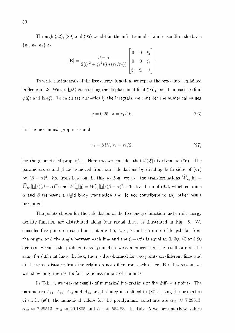
50

Through (82), (89) and (95) we obtain the innitesimal strain tensor E in the basis

e1, e2, e3 as

[E] =β − α

2(ξ12 + ξ2

2)(ln (r1/r2))

0 0 ξ1

0 0 ξ2

ξ1 ξ2 0

.To write the integrals of the free energy function, we repeat the procedure explained

in Section 4.3. We get h〈ξξξ〉 considering the displacement eld (95), and then use it to nd

ϕ〈ξξξ〉 and hd〈ξξξ〉. To calculate numerically the integrals, we consider the numerical values

ν = 0.25, δ = r1/16, (96)

for the mechanical properties and

r1 = 8Ul, r2 = r1/2, (97)

for the geometrical properties. Here too we consider that ω(|ξξξ|) is given by (86). The

parameters α and β are removed from our calculations by dividing both sides of (47)

by (β − α)2. So, from here on, in this section, we use the transformations Wx0 [h] =

Wx0 [h]/((β − α)2) and WL

x0[h] = W

L

x0[h]/(β − α)2. The last term of (95), which contains

α and β represent a rigid body translation and do not contribute to any other result

presented.

The points chosen for the calculation of the free energy function and strain energy

density function are distributed along four radial lines, as illustrated in Fig. 8. We

consider ve ponts on each line that are 4.5, 5, 6, 7 and 7.5 units of length far from

the origin, and the angle between each line and the ξ2−axis is equal to 0, 30, 45 and 90

degrees. Because the problem is axisymmetric, we can expect that the results are all the

same for dierent lines. In fact, the results obtained for two points on dierent lines and

at the same distance from the origin do not dier from each other. For this reason, we

will show only the results for the points on one of the lines.

In Tab. 4, we present results of numerical integrations at ve dierent points. The

parameters A11, A12, A33 and A13 are the integrals dened in (87). Using the properties

given in (96), the numerical values for the peridynamic constants are α11 ≈ 7.29513,

α12 ≈ 7.29513, α33 ≈ 29.1805 and α13 ≈ 554.83. In Tab. 5 we present these values

51

Figure 8: Points considered for the anti-plane shear problem.

Source: Own author

multiplied by the values of Tab. 4. The last two columns of Tab. 5 contain values of the

free energy function and the weighted average of the strain energy density. Comparing

these two columns, we see that, also for the anti-plane shear problem, the correspondence

argument (47) is approximately satised at the chosen points using the values given by

(96) and (97). Using (88), the maximum percentage error between the values of the two

columns is 0.017%, which is very small, in view of that the accuracy of the numerical

integration is limited.

Table 4: Results of numerical integrations for the anti-plane shear problem

(x0, y0) A11 A12 A33 A13

(0, 7.5) 0,00067655 0 0,000677064 2, 19175 · 10−9

(0, 7) 0,00077669 0 0,000777359 3, 26743 · 10−8

(0, 6) 0,00105733 0 0,0010586 5, 34805 · 10−8

(0, 5) 0,00152296 0 0,00152559 1, 18999 · 10−7

(0, 4.5) 0,00188057 0 0,00188449 1, 74136 · 10−7

Fig. 9 presents the numerical values for Wx0 [h] and WL

x0[h] along the axis (0, y0).

We can see that there is no visible dierence between the two graphs. Performing power

regression with the software NLREG for the data of Wx0 [h] and y0 from Tab. 5, we obtain

52

Wx0 [h] = 0.4221625 y0−2.0061641 and coecient of determination R2 = 0.99999986.

Table 5: Terms of free energy function and strain energy density for the anti-plane shear problem

(x0, y0) A11 · α11/2 A12 · α12 A33 · α33/4 A13 · α13/2 Wx0 [h] WL

x0[h]

(0, 7.5) 0,002468 0 0,004939 6, 0803 · 10−6 0,007413 0,007414

(0, 7) 0,002833 0 0,005671 9, 06435 · 10−6 0,008513 0,008513

(0, 6) 0,003857 0 0,007723 1, 48363 · 10−5 0,011594 0,011595

(0, 5) 0,005555 0 0,011129 3, 30121 · 10−5 0,016718 0,016718

(0, 4.5) 0,00686 0 0,013748 4, 83078 · 10−5 0,020655 0,020659

Figure 9: Numerical values of Wx0 [h] and WLx0

[h] plotted for points on the ξ2−axis in Fig. (8).

Source: Own author

53

5 PERIDYNAMIC BAR

In this section, we consider linear elastic peridynamic bars of nite length being

pulled at the ends and having micromoduli introduced by authors cited in Section 2.2.

We formulate the problem of a cylindrical bar in equilibrium without body force being

subjected to imposed displacements at its ends. Then we present the numerical scheme

used to obtain approximate solutions for the problem. We concentrate our attention on

a particular micromodulus that yields a singular behavior of the solution near the ends

and study both convergence of the proposed numerical scheme and convergence of the

nonlocal model to the classical linear elastic model as the horizon δ tends to zero.

5.1 1-D peridynamic model

To arrive at a one-dimensional peridynamic theory for a cylindrical bar of nite

length and constant cross-sectional area A, we start by assuming that the generators of

the bar are parallel to the x-axis. We then integrate the vector equation (9) over the

cross section A at an arbitrary coordinate ξ1 and divide the resulting expression through

by A. We further assume that the only non-zero equation that results from the above

consideration is given by

ρu(x) =

L+δ∫−δ

f(x, x)dx+ b(x),

where

u(x) =1

A

∫Au1(x)dA, b(x) =

1

A

∫Ab1(x)dA,

and

f(x, x) =1

A

∫A

∫Nf1(x, x)dA′dA, (98)

in which u1, b1 and f1 are the longitudinal components of u, b and f , respectively, and

dvξ = dAdx has been used.

The scalar force between particles, given by f in (98) is related to their relative

displacements through the constitutive relation

f(x, x) = f(u(x)− u(x), x− x), (99)

54

where the constitutive response function f satises

f(η, ξ) = −f(−η,−ξ), ∀ η, ξ,

so that Newton's third law is identically satised.

In this work we consider linear elastic peridynamic materials, so that

f(η, ξ) = C(ξ)η, (100)

where C is the micromodulus of the material and is analogous to the Young's modulus of

classical linear elasticity. In the next two sections we present dierent expressions of C

in terms of E that are found in the literature.

To satisfy (99), we require that C(ξ) = C(−ξ). In addiction we consider that

C(ξ) = 0 for |ξ| > δ, where δ is the horizon.

5.2 Finite bar pulled at the ends

Let [0, L] be the interval occupied by an one-dimensional bar in its natural state.

The bar is made of the linear peridynamic material given by (100). Because of the nonlocal

behavior of the bar, we extend the interval of denition of the axial displacement u to

[−δ, L+ δ], in such a way that boundary conditions are prescribed on the intervals [−δ, 0]

and [L,L+ δ].

The equilibrium equation without body force at a point x ∈ (0, L) of the peridy-

namic bar may be written as

L+δ∫−δ

C(x′ − x)[u(x′)− u(x)]dx′ = 0 , ∀x ∈ [0, L] . (101)

On the extended parts of the bar, we impose displacement boundary conditions, so that

u(x′) = u(x′) for x′ ∈ [−δ, 0]⋃

[L,L+ δ] . (102)

We then have that the problem of equilibrium without body force of the peridynamic

bar consists of nding the axial displacement u : (0, L) → R that satises the governing

equation (101) together with the boundary conditions given by (102). In Fig. 10 we

55

ilustrate the bar being pulled by a constant displacement ∆. In this case, u(x′) = 0 for

x′ ∈ [−δ, 0] and u(x′) = ∆ for x′ ∈ [L,L+ δ].

Figure 10: Finite bar of length L pulled at the ends with imposed displacement ∆.

Source: Own author

Now, let

C0 =

δ∫−δ

C(ξ)dξ (103)

and observe from (101) that

0 =

L+δ∫−δ

C(x′ − x)u(x′)dx′ − C0 u(x) =

L∫0

C(x′ − x)u(x′)dx′ − C0 u(x)+

0∫−δ

C(x′ − x)u(x′)dx′ +

L+δ∫L

C(x′ − x)u(x′)dx′ .

This can be rewritten in the form

u(x)− 1

C0

L∫0

C(x′ − x)u(x′)dx′ =g(x)

C0

, ∀x ∈ (0, L) , (104)

where

g(x) =

0∫−δ

C(x′ − x)u(x′)dx′ +

L+δ∫L

C(x′ − x)u(x′)dx′ . (105)

The integral equation (104) together with (105) yield an inhomogeneous Fredholm

equation of the second kind, where the role of the kernel is played by the micromodu-

lus function and the function g(x) depends only on the boundary data. Conditions for

existence of solutions are associated with the form of the kernel (PORTER; STIRLING,

56

1990). Granted that a solution exists, the equation can be easily solved numerically. Re-

call from a comment in Section 2.2 that a Fourier transform technique is used to nd a

closed form solution for the case of innite domains.

In the case of constant micromodulus function, given by

C(ξ) =

3E/δ3 if |ξ| ≤ δ ,

0 if |ξ| > δ ,

(106)

where E is the Young's modulus, and assuming that the boundary conditions are given

by

u(x) =

0 if x ∈ (−δ, 0) ,

∆ if x ∈ (L,L+ δ) ,

(107)

one nds from (103) that C0 = 6E/δ2 and from (105) that

g(x) =

0 if 0 ≤ x < L− δ ,

3E∆δ3

(x− L+ δ) if L− δ ≤ x ≤ L .

5.3 Numerical results and Discussion

We show numerical results for the four expressions of micromoduli presented below.

C(ξ) =

3E/δ3 (constant micromodulus),

[4E/(δ3√π)] e−(ξ/δ)2 (exponencial micromodulus),

(12E/δ3)(1− |ξ|/δ) (triangular micromodulus),

(6E/δ2)(1− |ξ|/δ)/|ξ| (singular micromodulus).

(108)

In all cases, the micromoduli are proportional to E in the interval (−δ, δ) and zero el-

sewhere. It follows from either (101) or (104) together with both (103) and (105) that the

numerical results do not depend on the value of E and, therefore, this value will be ig-

nored in the following computations. Also, the expression for the constant micromodulus

is the same one given by (106). The references where, to the best of our knowledge, the

corresponding expression rst appeared are Silling, Zimmermann e Abeyaratne (2003) for

constant micromodulus, Weckner, Brunk e Epton (2009) for exponencial micromodulus,

57

and Bobaru et al. (2009) for the singular micromodulus. The triangular micromodulus is

introduced in this work.

The graphs of the micromoduli given by (108) are presented in Fig. 11. Notice

that the three limited micromoduli are normalized to have C(0) = 1 and for all of them

C(ξ) = 0 if |ξ| > δ. We can see from the gure that the triangular micromodulus is

continuous and piecewise linear, both constant and exponencial micromoduli are smooth

at the origin, and discontinuous at ±δ, and the singular micromodulus is continuous,

except at the origin.

Figure 11: Shape of the micromodulus functions, C(ξ), for |ξ| ≤ δ.

Source: Own author

The particularly simple form of the expression (101) allows a straightforward im-

plementation of a numerical scheme, which can be extended to higher dimensions, for the

numerical calculation of the displacement eld of the peridynamic bar. An alternative

numerical scheme1, based on the Fredholm equation (104) together with both (103) and

(105), has also been implemented, but will not be presented here. Considering the boun-

dary conditions (107), we rst introduce the new variables x→ xL and u→ u/∆, where,

now, x ∈ (0, 1) and u(x) ∈ (0, 1), into (101) and rewrite this expression as

1+δ∫−δ

C((x′ − x)L)[u(x′)− u(x)]dx′ = 0 , ∀x ∈ [0, 1] . (109)

1The scheme is based on a computational code available at <http://mathematica.stackexchange.com/questions/104667/solving-fredholm-equation-of-the-2nd-kind>, which is written in the programMathematica R©.

58

where we have introduced the denition δ → δ L.

In the simplest approach, one can divide the interval (−δ, 1 + δ) into N + 1 + 2n

equidistant nodes such that x−n = −δ, x0 = 0, xN = 1 and xN+n = 1 + δ. We then have

that the distance between nodes is constant and given by h = 1/N = δ/n and that the

discretized form of the equilibrium equation (109) becomes the system of N +1 equations

N+n∑j=−n

C((xi − xj)L)[u(xi)− u(xj)]h = 0 , i = 0, ..., N . (110)

In Fig. 12 we illustrate the discretized bar and the boundary conditions. In this work

we consider geometric sequences of nodes starting with both N = 1000 and n = 20 and

having a factor of 2. Substituting C(ξ), given by one of the expressions in (108), into the

system of equations (110), we can solve for u(xi), i = 0, . . . , N , and obtain an approximate

expression for the displacement eld u(x).

Figure 12: Representation of the discretized bar and boundary conditions.

Source: Own author

To investigate the inuence of the horizon δ on the solution of the integral equation

(101), we consider the constant micromodulus given by either (106) or the rst expression

in (108) and the four horizons δ = 1/2, 1/5, 1/10, 1/50. In Fig. 13 we show the

displacement u(x) plotted against the position x ∈ (0, 1) for these four horizons and

N = 16000 nodes, which corresponds to the most rened mesh in this work. We see from

this gure that (i) the end points of the graphs tend to the points (0, 0) on the left end

and (1, 1) on the right end of the bar as δ decreases; (ii) the solution is highly nonlinear in

boundary layers of length δ near the ends and almost linear outside these boundary layers.

In fact, the sequence of solutions tends to the solution of the corresponding problem in

the classical linear elasticity theory as δ → 0, which is linear and satises the boundary

conditions exactly. This classical solution is represented by the thin solid line in the gure.

Thus, we see from these observations that displacement discontinuities appear at

the ends of the bar for a xed δ > 0. The jumps are nite and decrease as the horizon

decreases. Displacement discontinuities have already been observed for innite peridyna-

59

Figure 13: Displacement u(x) versus position x ∈ (0, 1) obtained from classical linear elasticity

and from peridynamics for the constant micromodulus, N = 16000, and four values of the horizonδ.

Source: Own author

mic bars under concentrated loads (SILLING; ZIMMERMANN; ABEYARATNE, 2003;

WECKNER; ABEYARATNE, 2005; MIKATA, 2012), but have not been reported yet for

nite bars subjected to displacement conditions at the ends.

The reason for the formation of the discontinuities is clear from the analysis of the

eld equation (109), which expresses, for each particle x ∈ (0, 1) and the corresponding set

of particles in its δ-neighborhoood, the equilibrium of the forces exerted by the particles

on the left- and right-hand sides of x. Thus, for a particle at x = 0, the particles on the

interval (−δ, 0) cannot move and the resultant of the forces on the left hand side must

be in equilibrium with the forces on the right-hand side, producing a strain localization.

Then, as x→ 0+, we have from the left-hand side that

∫ 0

−δC((x′ − x)L)[u(x′)− u(x)]dx′ = −[3E/(δ L)3]u(x) δ

and from the right-hand side that

∫ δ

0

C(x′ − x)[u(x′)− u(x)]dx′ = [3E/(δ L)3] (

∫ δ

0

u(x′)dx′ − u(x) δ).

We then have that u(0+) =∫ δ

0u(x′)dx′/(2 δ), that is, as we approach the origin from the

right-hand side, the value of u(x) is half of the average of the displacement eld evaluated

on the right-hand side of the origin. An analogous argument holds for x→ 1.

We now show that the eld equation (109) converges to the second order ordinary

60

dierential equation of classical linear elasticity as δ → 0 for the case of the constant

micromodulus. Such demonstration is usually done by using linear displacements as test

functions (SILLING; ZIMMERMANN; ABEYARATNE, 2003; MIKATA, 2012). Here,

however, it is done directly. For x ∈ (0, 1), straightforward applications of the l'Hôpital

rule yield

0 = L3 limδ→0

1+δ∫−δ

C((x′ − x)L)[u(x′)− u(x)]dx′ = limδ→0

3E

δ3

( x+δ∫x−δ

u(x′)dx′ − 2δu(x))

= limδ→0

E

δ2

([u(x+ δ)− u(x− δ)]− 2u(x)

)= lim

δ→0

E

2δ[u′(x+ δ)− u′(x− δ)]

= limδ→0

E

2[u′′(x+ δ) + u′′(x− δ)] = Eu′′(x) .

Next, we consider the four micromoduli given by (108), the horizon δ = 1/50 and

N = 16000 nodes, which corresponds to the most rened mesh in this work. Because of

the relation 1/N = δ/n introduced above, we have that n = 320 nodes. We then show in

Fig. 14 the displacement u(x) plotted against the reference position x ∈ (0, 0.006). For

comparison purposes, we also show a graph for the displacement u(x) obtained from the

exact solution of the bar problem in the context of the classical linear elasticity theory.

Observe from this gure that all the curves obtained from peridynamics are above the

curve obtained from the classical theory, are almost parallel to each other away from

the origin, and tend to dierent values as we approach the origin from its right-hand

side. Following arguments that are similar to those presented above in the analysis of the

constant micromodulus case, we have veried that these values are approximations of the

expression

u(0+) =

δ∫0

C((x′ − x)L)u(x′)dx′/(

2

∫ δ

0

C((x′ − x)L) dx′).

In the case of the singular micromodulus, we can rewrite this expression in the form

u(0+) =

δ∫0

C((x′ − x)L) [u(x′)− u(0+)]dx′/∫ δ

0

C((x′ − x)L) dx′ ,

and, provided that u(0+) is nite, observe that the integrand in the numerator is less

singular than the integrand in the denominator, which tends to innity as x→ 0+. Thus,

61

Figure 14: Displacement u(x) versus position x ∈ (0, 0.006) obtained from classical linear elasti-

city and from peridynamics for δ = 1/50, N = 16000, and four dierent micromoduli C.

Source: Own author

we have that u(x)→ 0 as x→ 0+.

To see the dierence on the behavior of the solution for dierent micromoduli near

the ends, we have considered a node at x > 0 and its immediate neighbor on its right-hand

side and evaluated the relative position ∆x between the two nodes as well as their relative

displacement ∆u(x) using peridynamics for the xed values δ = 1/50 and N = 16000 and

the four micromoduli shown in Fig. 14. We have then obtained Fig. 15 showing graphs of

the ratio ∆u(x)/∆x versus x ∈ (0, 0.002) for the dierent micromoduli. We see from the

gure that three of the curves are very similar, corresponding to ratios that are almost

constant and tend to a nite value as x tends to zero. For the singular micromodulus the

ratio ∆u(x)/∆x seems to become unbounded as x tends to zero.

From now on, we consider the singular micromodulus only, which is given by the

last expression in (108). To investigate convergence of the numerical scheme, we show

in Fig. 16 the displacement u(x) plotted against the reference position x ∈ (0, 0.003)

for increasing numbers of nodes and for the horizon δ = 1/50. Again, for comparison

purposes, we also show the graph of u(x) versus x obtained from the exact solution of

the bar problem in the context of the classical linear elasticity theory. We see from this

gure that all the curves obtained from peridynamics are nearly parallel to the curve

obtained from the classical linear theory away from the origin, the displacement elds

obtained from peridynamics converge to a limit eld as the number of nodes increases

62

Figure 15: Ratio between relative displacement ∆u(x) and relative position ∆x versus posi-

tion x ∈ (0, 0.002) obtained from peridynamics for δ = 1/50, N = 16000, and four dierent

micromoduli.

Source: Own author

geometrically, and this limit eld seems to have unbounded derivative at x = 0.

Figure 16: Displacement u(x) versus position x ∈ (0, 0.003) obtained from classical linear elasti-

city and from peridynamics for the singular micromodulus, δ = 1/50, and an increasing number

of nodes N .

Source: Own author

To see the last feature above more clearly, we have evaluated a more detailed

version of the ratio between ∆u(x) and ∆x corresponding to the singular micromodulus

in Fig. 15, in which we can see the convergence of the numerical scheme, using the values

of N shown in Fig. 16. We have then obtained Fig. 17 showing graphs of the ratio

63

∆u(x)/∆x versus x ∈ (0, 0.003) for the xed value δ = 1/50 and increasing values of

N . A diamond symbol on a curve yields the position of the rst node to the right of

the origin corresponding to a discretization with the number of nodes shown next to the

symbol. We then see from the gure that all the curves are on the top of each other for

x ≥ 0.001, which corresponds to the position of the rst node in a discretization with 1000

nodes. We also see that the ratio ∆u(x)/∆x becomes unbounded as the mesh becomes

rened, with the curves corresponding to less rened meshes being indistinguishable from

the curve corresponding to a more rened mesh.

Figure 17: Ratio between relative displacement ∆u(x) and relative position ∆x versus position

x ∈ (0, 0.003) obtained for the singular micromodulus, δ = 1/50, and increasing number of nodes

N .

Source: Own author

In Fig. 18 we hold N = 16000 xed and show the displacement u(x) plotted

against the reference position x ∈ (0, 1) for decreasing values of the horizon δ. Again, for

comparison purposes, we also show the graph of u(x) versus x obtained from the classical

linear elasticity theory. Observe from this gure that the peridynamic solutions tend to

the classical solution as δ decreases. To investigate the behavior of these curves near the

origin, we have plotted Fig. 19, which shows u(x) against x in the interval (0, 0.006).

Observe from this gure that u(x) obtained from peridynamics is highly nonlinear near

the origin, tends to u(x) obtained from classical theory as δ → 0, and, as observed earlier,

seems to have unbounded derivative at x = 0.

64

Figure 18: Displacement u(x) versus position x ∈ (0, 1) obtained from classical linear elasticity

and from peridynamics using N = 16000 and decreasing values of the horizon δ.

Source: Own author

Figure 19: Displacement u(x) versus position x ∈ (0, 0.006) obtained from classical linear elasti-

city and from peridynamics using N = 16000 and decreasing values of the horizon δ.

Source: Own author

65

6 CONCLUSIONS

Three of the four peridynamic constants that appear in the free energy function

dened by (18) were previously determined in Aguiar e Fosdick (2014) and Aguiar (2016).

From (39) it is noted that, to determine the fourth constant α13, we need to consider a

deformation state in which both hd and ϕ do not vanish. Considering the pure bending

experiment and using the correspondence argument between the free energy function and

the weighted average of the strain energy density function from classical elasticity theory,

in the form of (47), we obtain a relation between α13 and the elastic constants from

classical theory, which is given by (67).

We have veried the validity of the closed form expressions for the peridynamic

constants by using displacement elds from classical linear elasticity for both beam bent

by terminal loads and circular shaft subjected to anti-plane shear experiments. We set

numerical values for the material and geometrical properties and use the expressions

for the peridynamic constants to numerically calculate the free energy function and the

weighted average of the strain energy density function at selected points in the domain.

The results shown in Tab. 3, Tab. 5, Fig. 6 and Fig. 9 show that the correspondence

argument is nearly satised for the above experiments.

We have also investigated the one-dimensional problem of a linear elastic peridyna-

mic bar of length L being pulled at the ends by imposed displacements on extended parts

of the bar having length δ. We have shown that the problem can be formulated in terms

of an inhomogeneous Fredholm equation of the second kind, which assumes a simple form

in the case of a constant micromodulus. We have then used a numerical scheme to obtain

approximate solutions for the peridynamic problem using dierent expressions of micro-

modulus, horizons, and discretizations. Except for the singular micromodulus, all the

other micromoduli yield discontinuous displacements at the ends of the bar. Discontinu-

ous displacements have been reported in the study of innity bars, but not of nite bars.

The singular micromodulus gives continuous displacements, but unbounded derivatives of

displacements, at these ends. We have then focused our attention in the investigation of

this singular case and found that the approximate solutions of the peridynamic problem

converge to the classical solution of linear elasticity for vanishing horizon and a xed dis-

cretization. Also, for a xed horizon, these solutions converge to a limit function as the

mesh is rened. The information obtained from the investigation of the one-dimensional

66

peridynamic problem can now be applied to better understand the behavior of solutions

in higher dimensions and to design eective numerical schemes for higher-dimensional

problems.

67

REFERENCES

AGUIAR, A. On the determination of a peridynamic constant in a linear constitutivemodel. Journal of Elasticity, v. 122, p. 2739, 2016.

AGUIAR, A.; FOSDICK, R. A constitutive model for a linearly elastic peridynamicbody. Mathematics and Mechanics of Solids, v. 19, n. 5, p. 502523, 2014.

AGUIAR, A. R. Uma contribuição ao desenvolvimento da teoria peridinâmica. 2015. 100p. Free teaching Thesis - Department of Structural Engineering, São Carlos School ofEngineering, University of São Paulo, São Paulo. 2015.

ASKARI, E.; XU, J.; SILLING, S. Peridynamic analysis of damage and failure incomposites. In: 44th AIAA Aerospace Sciences Meeting and Exhibit. 2006.

BOBARU, F. et al. Convergence, adaptive renement, and scaling in 1d peridynamics.International Journal for Numerical Methods in Engineering, v. 77, n. 6, p. 852877,2009.

DAYAL, K.; BHATTACHARYA, K. Kinetics of phase transformations in the peridynamicformulation of continuum mechanics. Journal of the Mechanics and Physics of Solids,v. 54, n. 9, p. 18111842, 2006.

DIYAROGLU, C. et al. Peridynamic modeling of composite laminates under explosiveloading. Composite Structures, v. 144, p. 1423, 2016.

ERINGEN, A. C.; EDELEN, D. G. B. On nonlocal elasticity. International Journal ofEngineering Science, v. 10, n. 3, p. 233248, 1972.

ERINGEN, A. C.; KIM, B. S. Stress concentration at the tip of crack. Mechanics

Research Communications, v. 1, n. 4, p. 233237, 1974.

GERSTLE, W.; SAU, N.; SILLING, S. A. Peridynamic modeling of plain and reinforcedconcrete structures. In: International Conference on Structural Mechanics in ReactorTechnology, 18. Proceedings. . . , Beijing, China. 2005.

GLAWS, A. T. Finite element simulations of two dimensional peridynamic models. 2014.36 p. Dissertation (M. Sc. in Mathematics) - Faculty of the Virginia Polytechnic Instituteand State University, Virgínia, EUA. 2014.

GRIFFITH, A. A. The phenomena of rupture and ow in solids. PhilosophicalTransactions of the Royal Society of London A, v. 221, n. 582-593, p. 163198, 1921.

HA, Y. D.; LEE, J.; HONG, J. Fracturing patterns of rock-like materials in compressioncaptured with peridynamics. Engineering Fracture Mechanics, v. 144, p. 176193, 2015.

HORGAN, C. Anti-plane shear deformations in linear and nonlinear solid mechanics.Society for Industrial and Applied Mathematics Review, v. 37, n. 1, p. 5281, 1995.

HU, W.; HA, Y. D.; BOBARU, F. Peridynamic model for dynamic fracture inunidirectional ber-reinforced composites. Computer Methods in Applied Mechanics and

Engineering, v. 217-220, p. 247261, 2012.

68

HU, W. et al. Impact damage on a thin glass plate with a thin polycarbonate backing.International Journal of Impact Engineering, v. 62, p. 152165, 2013.

KRONER, E. Elasticity theory of materials with long range cohesive forces. Journal ofSolids and Structures, v. 3, n. 5, p. 731742, 1967.

KUNIN, A. Elastic Media with Microstructure I: One-Dimensional Models. Berlin:Springer, 1982.

LEHOUCQ, R.; SILLING, S. Force ux and the peridynamic stress tensor. Journal ofthe Mechanics and Physics of Solids, v. 56, n. 4, p. 15661577, 2008.

LITTLEWOOD, D. J.; MISH, K.; PIERSON, K. Peridynamic simulation of damageevolution for structural health monitoring. Mechanics of Solids, Structures and Fluids,v. 8, p. 18, 2012.

MADENCI, E.; OTERKUS, E. Peridynamic theory and its applications. New York:Springer, 2014.

MIKATA, Y. Analytical solutions of peristatic and peridynamic problems for a 1dinnite rod. International Journal of Solids and Structures, v. 49, n. 21, p. 28872897,2012.

OTERKUS, E. Peridynamic theory for modeling three-dimensional damage growth in

metallic and composite structures. 2010. 208 p. Thesis (PhD in Aerospace Engineering) -Department of Aerospace and Mechanical Engineering, University of Arizona, Tucson,EUA. 2010.

OTERKUS, E.; BARUT, A.; MADENCI, E. Damage growth prediction from loadedcomposite fastener holes by using peridynamic theory. In: Structures, Structural

Dynamics and Materials Conference, 51, Orlando, Florida. Collection of technical papers,Orlando: AAIA. 2010.

OTERKUS, E.; GUVEN, I.; MADENCI, E. Impact damage assessment by usingperidynamic theory. Central European Journal of Engineering, v. 2, n. 4, p. 523531,2012.

PORTER, D.; STIRLING, D. Integral equations: a practical treatment, from spectral

theory to applications. Cambridge, UK: Cambridge University Press, 1990. v. 5.

SILLING, S. Reformulation of elasticity theory for discontinuities and long-range forces.Journal of the Mechanics and Physics of Solids, v. 48, n. 1, p. 175209, 2000.

SILLING, S. Linearized theory of peridynamic states. Journal of Elasticity, v. 99, n. 1,p. 85111, 2010.

SILLING, S. et al. Peridynamic states and constitutive modeling. Journal of Elasticity,v. 88, n. 2, p. 151184, 2007.

SILLING, S.; LEHOUCQ, R. Convergence of peridynamics to classical elasticity theory.Journal of Elasticity, v. 93, n. 1, p. 1337, 2008.

SILLING, S.; ZIMMERMANN, M.; ABEYARATNE, R. Deformation of a peridynamicbar. Journal of Elasticity, v. 73, n. 1-3, p. 173190, 2003.

69

SOKOLNIKOFF, I. S. Mathematical Theory of Elasticity. 2. ed. New York: McGraw-Hill,1956.

WANG, L.; XU, J.; WANG, J. Erratum to: Static and dynamic green's functions inperidynamics. Journal of Elasticity, v. 126, n. 1, p. 127127, 2017.

WANG, L.; XU, J.; WANG, J. Static and dynamic green's functions in peridynamics.Journal of Elasticity, v. 126, n. 1, p. 95125, 2017.

WARREN, T. L. et al. A nonordinary state-based peridynamic method to model solidmaterial deformation and fracture. International Journal of Solids and Structures, v. 46,n. 5, p. 11861195, 2009.

WECKNER, O.; ABEYARATNE, R. The eect of long-range forces on the dynamics ofa bar. Journal of the Mechanics and Physics of Solids, v. 53, n. 3, p. 705728, 2005.

WECKNER, O.; BRUNK, G.; EPTON, M. Green's functions in non-local three-dimensional linear elasticity. Proceedings of the Royal Society A, v. 465, n. 2111, p.34633487, 2009.

ZHOU, X.; GU, X.; WANG, Y. Numerical simulations of propagation, bifurcation andcoalescence of cracks in rocks. International Journal of Rock Mechanics and Mining

Sciences, v. 80, p. 241254, 2015.