algebra ii { commutative and homological algebra - bc.edu · pdf filealgebra ii { commutative...

Algebra II – Commutative and Homological Algebra

Spring 2016, lecture notes by Maksym Fedorchuk

Contents

1 Preliminaries 2

1.1 Cayley-Hamilton Theorem 2

1.2 Chain conditions 3

1.3 Noetherian rings 5

1.4 Weak Nullstellensatz 6

1.5 Algebraic sets and Hilbert’s Nullstellensatz 7

2 Spectrum of a ring 9

2.1 Zariski topology on SpecR 11

2.2 Operations on ideals 12

3 Localization 12

3.1 Localization at a prime 14

3.2 Modules 14

3.3 Local properties of modules 15

3.4 Extended and contracted ideals 15

3.5 Some remarks on morphisms of ring spectra 17

3.6 Some properties of integral extensions 18

3.7 Cohen-Seidenberg Theorems 19

4 Grobner bases 24

4.1 Elimination problem 24

5 Dimension Theory 25

5.1 Nakayama’s lemma 25

5.2 Artinian rings 25

5.3 Krull dimension 26

1

2 Algebra II – Commutative and Homological Algebra

1. Preliminaries

All rings are commutative and unital. The zero ring is the only ring in

which 0 = 1. Throughout ⊂ will stand for non-strict inclusion.

1.1. Cayley-Hamilton Theorem

Let R be a ring. Then an R-module M is finitely generated if it has

a finite set of generators, if and only if M is a quotient of a finite free module

Rn = R⊕ · · · ⊕R︸︷︷︸n

.

Suppose φ : R → S is a ring homomorphism (that is, S is an R-algebra).

Then we say that

• φ is finite type if S is a finitely generated R-algebra.

• φ is finite if S is a finitely generated R-module.

• An element t ∈ S is integral over R if it satisfies a monic polynomial

relation

tn + an−1tn−1 + · · ·+ a0 = 0

for some a0, . . . , an−1 ∈ R.

• φ is integral if all elements of S are integral over R.

Example 1.1.1. The polynomial algebra R[x1, . . . , xn] is a finitely generated R-

algebra, but not a finitely generated R-module if n ≥ 1.

Theorem 1.1.2 (Cayley-Hamilton). Suppose M is a finitely generated R-module.

Suppose I ⊂ R is an ideal of R and φ : M → M is an R-module endomorphism

such that φ(M) ⊂ IM . Then φ satisfies

φn + an−1φn−1 + · · ·+ a0 = 0 ∈ End(M)

for some a0, . . . , an−1 ∈ I.

Proof. Let m1, . . . ,mn be generators of M . (They exist by the finite generation

assumption.) Then for i = 1, . . . , n, we can write

φ(mi) = ci1m1 + · · ·+ cinmn,

where cij ∈ I. In other words, if A is an n×n matrix with coefficients in End(M)

with the entries

Aij =

{cij if i 6= j

cii − φ if i = j,

then A(m1, . . . ,mn)tr = (0, . . . , 0)tr. Multiplying on the left by the matrix of

cofactors of A, we obtain

det(A)m1 = · · · = det(A)mn = 0.

Hence det(A)M = 0 and expanding the determinant we get the desired claim. �

Spring 2016, lecture notes by Maksym Fedorchuk 3

Corollary 1.1.3. Suppose M is a finitely generated R-module such that IM = M

for some ideal I ⊂ R. Then there exists x ∈ R such that x ≡ 1 (mod I) and

xM = 0.

Proof. Take φ = 1M and x = 1+a1 + · · ·+an−1 in the Cayley-Hamilton Theorem.

�

Proposition 1.1.4. Suppose R ⊂ S is a ring extension. Then the following are

equivalent:

(1) t ∈ S is integral over R.

(2) R[t] is a finitely generated R-module.

(3) R[t] is contained in a subring Q of S such that Q is a finitely generated

R-module.

Proof. (1)⇒ (2): Suppose

tn + an−1tn−1 + · · ·+ a0 = 0.

Then R[t] is generated by 1, t, . . . , tn−1 as an R-module.

(2)⇒ (3): Obvious (take Q = R[t]).

(3) ⇒ (1): Let φ : Q → Q be an R-module endomorphism given by the

multiplication by t, that is φ(a) = ta for every a ∈ Q. Then by the Cayley-

Hamilton Theorem applied with I = R, we have

tn + an−1tn−1 + · · ·+ a0 = 0 ∈ End(Q).

Applying the above zero endomorphism to 1 ∈ Q, we obtain

tn + an−1tn−1 + · · ·+ a0 = 0

as an element in Q, and hence in S. (The point here is that Q is a faithful

R-module because it is also an R-algebra.) �

N.B. In general, a submodule of a finitely generated module does not have

to be finitely generated, so the implication (3)⇒ (2) has some non-trivial content.

Corollary 1.1.5. A ring homomorphism φ : R → S is finite if and only if φ is

finite type and integral.

Proof. Exercise; see Problem Set 1. �

1.2. Chain conditions

Let Σ be a non-empty partially ordered set with relation ≤.

Axiom (Zorn’s lemma). Suppose Σ has the property that every totally ordered

subset S ⊂ Σ has an upper bound1. Then Σ has a maximal element.

1An upper bound of S is an element u ∈ Σ satisfying x ≤ u,∀x ∈ S.

https://en.wikipedia.org/wiki/Partially_ordered_set#Formal_definition


Corollary 1.2.1. For every proper ideal I ( R, there is a maximal ideal contain-

ing it. In particular, every non-unit element f ∈ R is contained in some maximal

ideal of R.

Proof. Consider the set {J : J ( R is an ideal and I ⊂ J} with a partial ordering

J1 ≤ J2 if J1 ⊆ J2. Every totally ordered subset {Jλ}λ∈S has an upper bound⋃λ∈S

Jλ. The statement follows. �

Lemma 1.2.2. The following are equivalent:

(1) Every increasing sequence x1 ≤ x2 ≤ · · · in Σ is stationary (that is,

xn = xn+1 = · · · for some n).

(2) Every non-empty subset of Σ has a maximal element.

Proof. Exercise. �

Let M be an R-module and Σ be the set of submodules of M . If Σ is ordered

by inclusion ⊂, then Condition (1) in the above lemma is called the ascending

chain condition, or a.c.c. If Σ is ordered by ⊃, then Condition (1) is called the

desceding chain condition, or d.c.c.

Definition 1.2.3. An R-module M is called Noetherian (resp., Artinian) if M

satisfies a.c.c. (resp., d.c.c.).

Lemma 1.2.4. An R-module M is Noetherian if and only if every2 submodule of

M is finitely generated.


Example 1.2.5. Every finite abelian group is both Artinian and Noetherian as a

Z-module.

Example 1.2.6. Z is a Noetherian, but not Artinian, Z-module.

Example 1.2.7. Let U =

{m

pn| m,n ∈ Z

}⊂ Q and W = U/Z. Then W is an

Artinian, but not Noetherian, Z-module. See Problem Set 1.

Lemma 1.2.8. Suppose 0 → M ′ → M → M ′′ → 0 is a short exact sequence of

R-modules. Then M is Noetherian (resp., Artinian) if and only if M ′ and M ′′

are Noetherian (resp., Artinian).


It follows from the above lemma that finite direct sums and finite internal

sums of Noetherian (resp., Artinian) modules are also Noetherian (resp., Artinian).

2N.B. This includes M itself.


1.3. Noetherian rings

Definition 1.3.1. A ring R is Noetherian (resp., Artinian) if R is Noetherian

(resp., Artinian) as an R-module.

Lemma 1.3.2. The following are equivalent for a ring R:

(1) R is a Noetherian ring.

(2) All ideals of R are finitely generated.

(3) Ideals of R satisfy a.c.c.

(4) Every non-empty set of ideals has a maximal element.

Proof. This follows from the definitions and Lemmas 1.2.2 and 1.2.4. �

Example 1.3.3. Every PID is a Noetherian ring.

Example 1.3.4. Let R be a PID and p ∈ R be an irreducible element. Then

R/(pn) is an Artinian ring for every n ≥ 1.

Example 1.3.5. Let R be a non-zero ring. Then R[x1, x2, . . . ] (infinite number

of variables) is not a Noetherian ring.

N.B. In contrast to the situation with modules, where Noetherian and Ar-

tinian conditions are independent, every Artinian ring is also Noetherian. This is

a non-trivial theorem, which we will revisit in the future.

Lemma 1.3.6. Suppose R is a Noetherian ring. Then an R-module M is Noe-

therian if and only if M is finitely generated.


Definition 1.3.7. Let I ⊂ R be an ideal. A prime ideal p is called a minimal

prime of I if there are no prime ideals strictly contained in p and containing I.

A minimal prime of the zero ideal (0) is called a minimal prime ideal.

If p is a minimal prime of I, we also say that p is a minimal prime over I.

Lemma 1.3.8. Every ideal has at least one minimal prime over it.


Proposition 1.3.9. Let R be a Noetherian ring. Then every ideal has finitely

many minimal prime ideals.

Proof. Suppose not. Let I be the maximal ideal with infinitely many primes over

it. Then I is not prime, and so there exist f, g /∈ I such that fg ∈ I. Clearly, every

prime ideal containing I must contain either (I, f) or (I, g). It follows that every

minimal prime of I is either a minimal prime over (I, f) or a minimal prime over

(I, g). But both (I, f) and (I, g) have finitely many primes by the maximality of

I. A contradiction! �


Theorem 1.3.10 (Hilbert’s Basis Theorem). Let R be a Noetherian ring. Then

R[x] is also Noetherian.

Theorem 1.3.11. Let R be a Noetherian ring. Then R[[x]] is also Noetherian.

Corollary 1.3.12. Let R be a Noetherian ring and S be a finitely generated R-

algebra. Then S is Noetherian.

Proof. We have that S is a quotient of some polynomial ring R[x1, . . . , xn], which

is Noetherian by a repeated application of the Hilbert Basis Theorem. �

Proposition 1.3.13 (Artin-Tate). Suppose A ⊂ B ⊂ C are rings. Suppose A is

Noetherian and C is a finitely generated A-algebra. Assume further that C is a

finitely generated B-module. Then B is a finitely generated A-algebra.

N.B. By Corollary 1.1.5, under the assumptions of the proposition, the con-

dition that B ⊂ C is finite is equivalent to the condition that B ⊂ C is integral.

Proof. Let x1, . . . , xm be generators of C as an A-algebra. Let y1, . . . , yn be gen-

erators of C as a B-module. Then we have

for every i = 1, . . . ,m, xi =

n∑j=1

bi,j yj , where bi,j ∈ B,(1.3.14)

for every i, j = 1, . . . , n, yiyj =

n∑k=1

bi,j,k yk, where bi,j,k ∈ B.(1.3.15)

Every element of C is a polynomial in x1, . . . , xm with coefficients in A. Using Rela-

tions (1.3.14) and (1.3.15), we can write every element of C as a linear combination

of y1, . . . , yn with coefficients in

B0 := A[{bi,j}m,ni,j=1, {bi,j,k}

ni,j,k=1

].

Since B0 is a finitely generated A-algebra, we have that B0 is a Noetherian

ring (by Corollary 1.3.12). Since C is a finitely generated B0-module, we conclude

that C is a Noetherian B0-module (by Lemma 1.3.6). Since B is a B0-submodule

of C, we conclude that B is a finitely generated B0-module. Together with the fact

that B0 is a finitely generated A-algebra, this proves that B is a finitely generated

A-algebra. �

1.4. Weak Nullstellensatz

We are going to apply Proposition 1.3.13 to obtain a description of the max-

imal ideals in the polynomial ring k[x1, . . . , xn], where k is a field.

Proposition 1.4.1 (Weak Nullstellensatz). Suppose k ⊂ K is a field extension

such that K is a finitely generated k-algebra. Then K is a finite field extension of

k.


Proof. Because a finitely generated algebraic field extension is finite, it suffices to

show that K/k is an algebraic extension. Suppose not. Then we can choose gen-

erators x1, . . . , xn of K as a k-algebra so that x1, . . . , xr (r ≥ 1) are algebraically

independent over k, but xr+1, . . . , xn are algebraic over the field k(x1, . . . , xr). Set

F := k(x1, . . . , xr). Then K is algebraic over F , and so by Proposition 1.3.13, the

field F must be a finitely generated k-algebra.

Suppose yj = fj/gj ∈ F , where fj , gj ∈ k[x1, . . . , xr] for j = 1, . . . , s, gener-

ate F as a k-algebra. Using the fact that k[x1, . . . , xr] is a UFD, it is easy to see

that1

g1 · · · gs + 1/∈ k[y1, . . . , yn] = F.

A contradiction! �

Corollary 1.4.2. Let R = k[x1, . . . , xn]/I. If k is algebraically closed, then every

maximal ideal of R is of the form (x1 − a1, . . . , xn − an), where xi is the image of

xi in R and ai ∈ k satisfy

I ⊂ (x1 − a1, . . . , xn − an) ⊂ k[x1, . . . , xn].

Proof. Let m be a maximal ideal of R. By the Weak Nullstellensatz (Proposition

1.4.1), we have that the field R/m is a finite field extension of k. Since k is alge-

braically closed, we conclude that R/m ' k. Note that this is also an isomorphism

of k-algebras! Let xi be the image of xi in R and let ai be the image of xi under the

quotient morphism R → R/m. Clearly, xi − ai ∈ m. Since (x1 − a1, . . . , xn − an)

is already maximal, we conclude that m = (x1 − a1, . . . , xn − an). The rest of

the statement follows from the fact that the preimage of (x1 − a1, . . . , xn − an) in

k[x1, . . . , xn] is (x1 − a1, . . . , xn − an). �

1.5. Algebraic sets and Hilbert’s Nullstellensatz

In this subsection, k is an algebraically closed field and R = k[x1, . . . , xn].

Consider the affine n-space

kn := {(a1, . . . , an) : ai ∈ k}.

By the Weak Nullstellensatz, the maximal ideals of R are identified with kn,

with the bijection given by

m = (x1 − a1, . . . , xn − an)↔ (a1, . . . , an).

Definition 1.5.1. The set

Z(I) = {(a1, . . . , an) : f(a1, . . . , an) = 0,∀f ∈ I} ⊂ kn

is called the algebraic set defined by I.


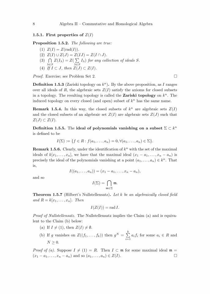
1.5.1. First properties of Z(I)

Proposition 1.5.2. The following are true:

(1) Z(I) = Z(rad(I)).

(2) Z(I) ∪ Z(J) = Z(IJ) = Z(I ∩ J).

(3)⋂λ∈S

Z(Iλ) = Z(∑λ∈S

Iλ) for any collection of ideals S.

(4) If I ⊂ J , then Z(J) ⊂ Z(I).


Definition 1.5.3 (Zariski topology on kn). By the above proposition, as I ranges

over all ideals of R, the algebraic sets Z(I) satisfy the axioms for closed subsets

in a topology. The resulting topology is called the Zariski topology on kn. The

induced topology on every closed (and open) subset of kn has the same name.

Remark 1.5.4. In this way, the closed subsets of kn are algebraic sets Z(I)

and the closed subsets of an algebraic set Z(I) are algebraic sets Z(J) such that

Z(J) ⊂ Z(I).

Definition 1.5.5. The ideal of polynomials vanishing on a subset Σ ⊂ kn

is defined to be

I(Σ) := {f ∈ R : f(a1, . . . , an) = 0,∀(a1, . . . , an) ∈ Σ}.

Remark 1.5.6. Clearly, under the identification of kn with the set of the maximal

ideals of k[x1, . . . , xn], we have that the maximal ideal (x1 − a1, . . . , xn − an) is

precisely the ideal of the polynomials vanishing at a point (a1, . . . , an) ∈ kn. That

is,

I((a1, . . . , an)) = (x1 − a1, . . . , xn − an),

and so

I(Σ) =⋂m∈Σ

m.

Theorem 1.5.7 (Hilbert’s Nullstellensatz). Let k be an algebraically closed field

and R = k[x1, . . . , xn]. Then

I(Z(I)) = rad I.

Proof of Nullstellensatz. The Nullstellensatz implies the Claim (a) and is equiva-

lent to the Claim (b) below:

(a) If I 6= (1), then Z(I) 6= ∅.

(b) If g vanishes on Z((f1, . . . , fk)) then gN =k∑i=1

aifi for some ai ∈ R and

N ≥ 0.

Proof of (a). Suppose I 6= (1) = R. Then I ⊂ m for some maximal ideal m =

(x1 − a1, . . . , xn − an) and so (a1, . . . , an) ∈ Z(I). �


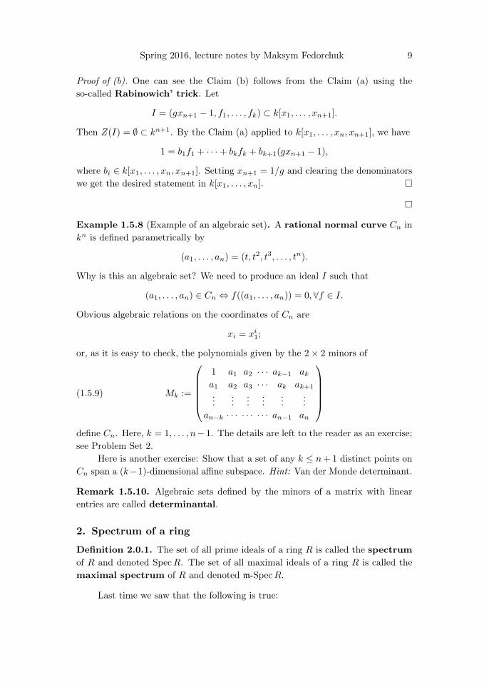
Proof of (b). One can see the Claim (b) follows from the Claim (a) using the

so-called Rabinowich’ trick. Let

I = (gxn+1 − 1, f1, . . . , fk) ⊂ k[x1, . . . , xn+1].

Then Z(I) = ∅ ⊂ kn+1. By the Claim (a) applied to k[x1, . . . , xn, xn+1], we have

1 = b1f1 + · · ·+ bkfk + bk+1(gxn+1 − 1),

where bi ∈ k[x1, . . . , xn, xn+1]. Setting xn+1 = 1/g and clearing the denominators

we get the desired statement in k[x1, . . . , xn]. �

�

Example 1.5.8 (Example of an algebraic set). A rational normal curve Cn in

kn is defined parametrically by

(a1, . . . , an) = (t, t2, t3, . . . , tn).

Why is this an algebraic set? We need to produce an ideal I such that

(a1, . . . , an) ∈ Cn ⇔ f((a1, . . . , an)) = 0,∀f ∈ I.

Obvious algebraic relations on the coordinates of Cn are

xi = xi1;

or, as it is easy to check, the polynomials given by the 2× 2 minors of

Mk :=

1 a1 a2 · · · ak−1 aka1 a2 a3 · · · ak ak+1

......

......

......

an−k · · · · · · · · · an−1 an

(1.5.9)

define Cn. Here, k = 1, . . . , n− 1. The details are left to the reader as an exercise;

see Problem Set 2.

Here is another exercise: Show that a set of any k ≤ n+ 1 distinct points on

Cn span a (k−1)-dimensional affine subspace. Hint: Van der Monde determinant.

Remark 1.5.10. Algebraic sets defined by the minors of a matrix with linear

entries are called determinantal.

2. Spectrum of a ring

Definition 2.0.1. The set of all prime ideals of a ring R is called the spectrum

of R and denoted SpecR. The set of all maximal ideals of a ring R is called the

maximal spectrum of R and denoted m-SpecR.

Last time we saw that the following is true:


Proposition 2.0.2. Suppose k is an algebraically closed field and that R =

k[x1, . . . , xn]/I is a finitely generated k-algebra. Then under the identification

of m-Spec k[x1, . . . , xn] with kn, we have

(2.0.3) m-SpecR = Z(I) = {(a1, . . . , an) ∈ kn | I ⊂ (x1 − a1, . . . , xn − an)}= {(a1, . . . , an) ∈ kn | f(a1, . . . , an) = 0, ∀f ∈ I}.

The algebraic set Z(I), with the induced Zariski topology, is called an affine

variety. Closed subsets of Z(I) are algebraic sets of the form Z(J), where I ⊂ J .

Definition 2.0.4. The coordinate ring of an affine variety X ⊂ kn is

k[X] := k[x1, . . . , xn]/I(X).

Definition 2.0.5. A variety X ⊂ kn is irreducible if it is nonempty and not the

union of two proper subvarieties; that is, if X = Z(I1) ∪ Z(I2), then X = Z(I1)

or X = Z(I2).

Proposition 2.0.6. A variety X ⊂ kn is irreducible if and only if I(X) ⊂k[x1, . . . , xn] is a prime ideal, or equivalently if and only if the coordinate ring

k[X] is an integral domain.

Proof. Suppose that X = Z(p) is reducible for a prime ideal p. Then X = Z(I1)∪Z(I2) with Z(Ii) 6= Z(p). It follows that p ( Ii. Therefore, ∃f ∈ I1 \ p and

∃g ∈ I2 \ p. Then fg vanishes on Z(I1) ∪ Z(I2) = X. Therefore fg ∈ I(X) = p.

A contradiction!

The other direction is similar and is left as an exercise; see Problem Set 2. �

Corollary 2.0.7. Suppose k is an algebraically closed field and that R = k[x1, . . . , xn]/I

is a finitely generated k-algebra. Then there is a one-to-one correspondence between

SpecR and the irreducible subvarieties of Z(I) ⊂ kn.


Proposition 2.0.8. Every variety X ⊂ kn has a decomposition

X = X1 ∪ · · · ∪Xr,

where each Xi is an irreducible closed subset.

Definition 2.0.9. The Xi’s are called irreducible components of X.

Proof. Suppose X = Z(I). Then since every ideal in k[x1, . . . , xn] has finitely

many minimal primes, we have

rad(I) =⋂

p is a minimal prime of I

p.

Therefore,

Z(I) = Z(rad(I)) =⋃

p is a minimal prime of I

Z(p).

�


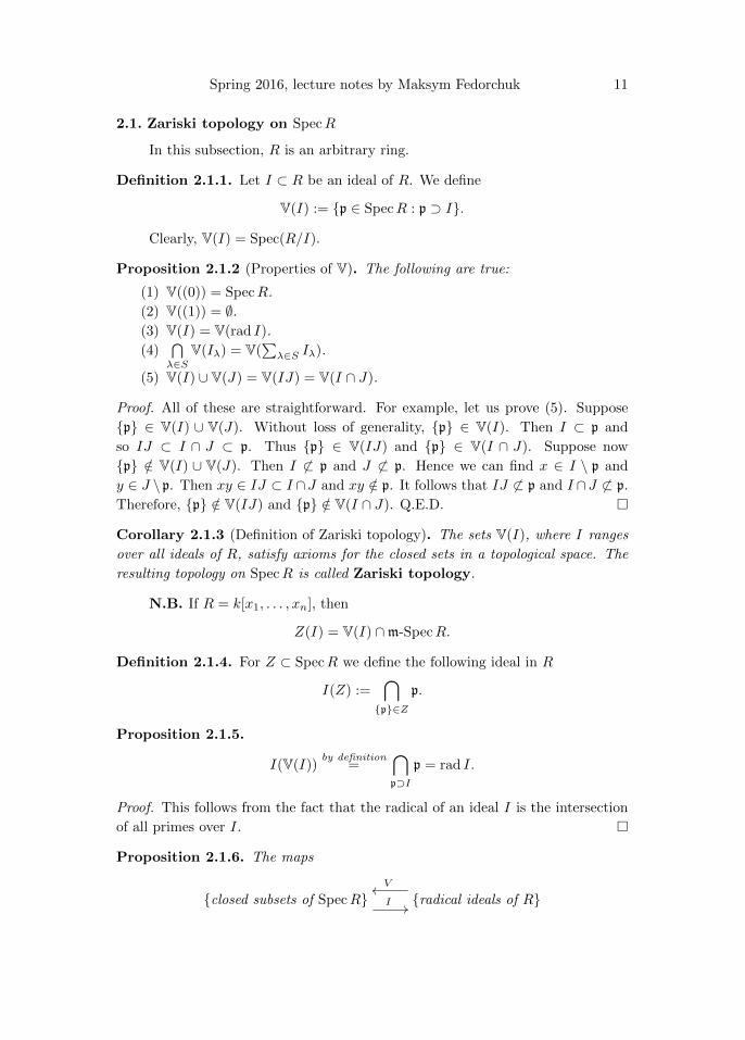
2.1. Zariski topology on SpecR

In this subsection, R is an arbitrary ring.

Definition 2.1.1. Let I ⊂ R be an ideal of R. We define

V(I) := {p ∈ SpecR : p ⊃ I}.

Clearly, V(I) = Spec(R/I).

Proposition 2.1.2 (Properties of V). The following are true:

(1) V((0)) = SpecR.

(2) V((1)) = ∅.(3) V(I) = V(rad I).

(4)⋂λ∈S

V(Iλ) = V(∑λ∈S Iλ).

(5) V(I) ∪ V(J) = V(IJ) = V(I ∩ J).

Proof. All of these are straightforward. For example, let us prove (5). Suppose

{p} ∈ V(I) ∪ V(J). Without loss of generality, {p} ∈ V(I). Then I ⊂ p and

so IJ ⊂ I ∩ J ⊂ p. Thus {p} ∈ V(IJ) and {p} ∈ V(I ∩ J). Suppose now

{p} /∈ V(I) ∪ V(J). Then I 6⊂ p and J 6⊂ p. Hence we can find x ∈ I \ p and

y ∈ J \ p. Then xy ∈ IJ ⊂ I ∩J and xy /∈ p. It follows that IJ 6⊂ p and I ∩J 6⊂ p.

Therefore, {p} /∈ V(IJ) and {p} /∈ V(I ∩ J). Q.E.D. �

Corollary 2.1.3 (Definition of Zariski topology). The sets V(I), where I ranges

over all ideals of R, satisfy axioms for the closed sets in a topological space. The

resulting topology on SpecR is called Zariski topology.

N.B. If R = k[x1, . . . , xn], then

Z(I) = V(I) ∩m-SpecR.

Definition 2.1.4. For Z ⊂ SpecR we define the following ideal in R

I(Z) :=⋂{p}∈Z

p.

Proposition 2.1.5.

I(V(I))by definition

=⋂p⊃I

p = rad I.

Proof. This follows from the fact that the radical of an ideal I is the intersection

of all primes over I. �

Proposition 2.1.6. The maps

{closed subsets of SpecR} I //{radical ideals of R}

Voo


are inverses of each other and define the inclusion-reversing bijection between the

closed subsets of SpecR and the radical ideals of R. Moreover, under this corre-

spondence, prime ideal of R correspond to prime ideals of R.

Proof. If I is radical, then I(V(I)) = rad(I) = I. Clearly, V(I(V(J))) = V(rad(J)) =

V(J). �

2.2. Operations on ideals

Suppose f : A→ B is a ring homomorphism.

Definition 2.2.1. The extension of an ideal I ⊂ A is the ideal f(I)B ⊂ B (also

denoted IB).

Definition 2.2.2. The contraction of an ideal J ⊂ B is the ideal f−1(J) ⊂ A

(also denoted J ∩A, even when f : A→ B is not an inclusion!)

The relevant ring homomorphisms on the quotient rings are

f : A/I → B/Bf(I)

f : A/f−1(J) = A/(A ∩ J) ↪→ B/J.

Proposition 2.2.3. The contraction of a prime ideal is prime.

Proof. Suppose J ⊂ B is prime. ThenB/J is an integral domain. SinceA/f−1(J) ↪→B/J is an injection, we conclude that A/f−1(J) is a domain and so f−1(J) is also

prime. �

Corollary 2.2.4. The contraction under the ring homomorphism f : A → B

defines a map of sets f ] : SpecB → SpecA.

Example 2.2.5. Can the contraction of a maximal ideal be non-maximal? Yes!

The contraction of a maximal ideal does not have to be a maximal ideal. For

example, if p ⊂ R is prime and R → Rp is a localization map then R ∩ Rp = p is

a prime but not necessarily maximal.

Proposition 2.2.6. Given a ring homomorphism f : R→ S, the map f ] : SpecS →SpecR is a continuous map in the Zariski topology.

Proof. We have that (f ])−1(V(I)) = V(Ie), for any ideal I ⊂ A. Indeed, observe

that f ]({p}) ∈ V(I) if and only if I ⊂ f−1(p) if and only if Ie = Sp ⊂ p. �

3. Localization

Definition 3.0.1. A subset S ⊂ R is called multiplicative set if 1 ∈ S and S is

closed under multiplication. A multiplicative set S is called saturated if

xy ∈ S ⇒ x, y ∈ S.


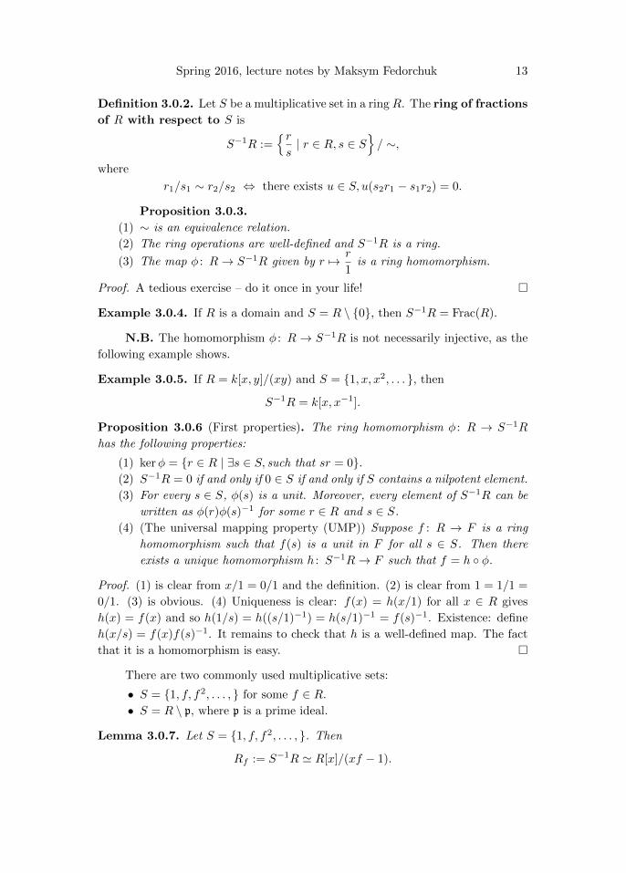
Definition 3.0.2. Let S be a multiplicative set in a ring R. The ring of fractions

of R with respect to S is

S−1R :={rs| r ∈ R, s ∈ S

}/ ∼,

where

r1/s1 ∼ r2/s2 ⇔ there exists u ∈ S, u(s2r1 − s1r2) = 0.

Proposition 3.0.3.

(1) ∼ is an equivalence relation.

(2) The ring operations are well-defined and S−1R is a ring.

(3) The map φ : R→ S−1R given by r 7→ r

1is a ring homomorphism.

Proof. A tedious exercise – do it once in your life! �

Example 3.0.4. If R is a domain and S = R \ {0}, then S−1R = Frac(R).

N.B. The homomorphism φ : R → S−1R is not necessarily injective, as the

following example shows.

Example 3.0.5. If R = k[x, y]/(xy) and S = {1, x, x2, . . . }, then

S−1R = k[x, x−1].

Proposition 3.0.6 (First properties). The ring homomorphism φ : R → S−1R

has the following properties:

(1) kerφ = {r ∈ R | ∃s ∈ S, such that sr = 0}.(2) S−1R = 0 if and only if 0 ∈ S if and only if S contains a nilpotent element.

(3) For every s ∈ S, φ(s) is a unit. Moreover, every element of S−1R can be

written as φ(r)φ(s)−1 for some r ∈ R and s ∈ S.

(4) (The universal mapping property (UMP)) Suppose f : R → F is a ring

homomorphism such that f(s) is a unit in F for all s ∈ S. Then there

exists a unique homomorphism h : S−1R→ F such that f = h ◦ φ.

Proof. (1) is clear from x/1 = 0/1 and the definition. (2) is clear from 1 = 1/1 =

0/1. (3) is obvious. (4) Uniqueness is clear: f(x) = h(x/1) for all x ∈ R gives

h(x) = f(x) and so h(1/s) = h((s/1)−1) = h(s/1)−1 = f(s)−1. Existence: define

h(x/s) = f(x)f(s)−1. It remains to check that h is a well-defined map. The fact

that it is a homomorphism is easy. �

There are two commonly used multiplicative sets:

• S = {1, f, f2, . . . , } for some f ∈ R.

• S = R \ p, where p is a prime ideal.

Lemma 3.0.7. Let S = {1, f, f2, . . . , }. Then

Rf := S−1R ' R[x]/(xf − 1).


Proof. Let F = R[x]/(xf − 1). We have that f is invertible in F with f−1 = x

and so by the UMP of S−1R, there exists a ring homomorphism

h : Rf → R[x]/(xf − 1),

such that h(r/fn) = rxn. Since R and x are in the image of h, we have that h

is surjective. Conversely, we have a ring homomorphism R[x] → Rf sending x

to 1/f , which is surjective and has (xf − 1) in its kernel. It follows that there

exists a ring homomorphism g : R[x]/(xf − 1) → Rf sending x to 1/f and R to

R. Clearly, g and h are inverses of each other. Q.E.D. �

3.1. Localization at a prime

Definition 3.1.1. Let p ∈ SpecR. Then S = R \ p is a multiplicative set. We

define the localization of R at p to be the ring

Rp := S−1R.

The elementsr

s, where r ∈ p and s /∈ p form an ideal in Rp, denoted pRp.

Every elements outside of this ideal is a unit. Hence pRp is the unique maximal

ideal of Rp.

Definition 3.1.2. A ring R with a unique maximal ideal m is called a local ring.

The common notation is (R,m). The quotient R/m is called the residue field of

R.

Remark 3.1.3. Observe that the residue field of Rp is the fraction field of R/p:

Rp/pRp = Frac(R/p).

3.2. Modules

If M is an R-module, the module of fractions of M with respect to S is

S−1M :={ms| m ∈ R, s ∈ S

}/(m1/s1 = m2/s2 ⇔ ∃u ∈ S, u(s2m1−s1m2) = 0

)S−1M is an S−1R-module via the obvious operations of addition and scalar mul-

tiplication.

For S = {1, f, f2, . . . }, we set Mf := S−1M , and for a prime ideal p ⊂ R, we

define the localization of M at p to be the module Mp := S−1M.

Given an R-module homomorphism u : M → N , we obtain an S−1R-module

homomorphism S−1u : S−1M → S−1N .

Proposition 3.2.1. The operation of forming the module of fraction with respect

to S−1 is exact:

M1f−→M2

g−→M3 is exact =⇒ S−1M1S−1f−→ S−1M2

S−1g−→ S−1M3 is exact.


Proof. We have S−1g ◦ S−1f = S−1(g ◦ f) = S−1(0) = 0. Hence it suffices to

show that kerS−1g ⊂ imS−1f . Suppose S−1g(m/s) = 0. Then g(m)/s = 0 in

S−1M3. Hence for some t ∈ S, we have tg(m) = 0 in M3. Then g(tm) = 0 and so

tm ∈ ker(g) = im(f). Write tm = f(m′). Then m/s = S−1f(m′/ts). �

Corollary 3.2.2. Formation of fractions commmutes with formation of finite

sums, finite intersections, and quotients.

Proposition 3.2.3. S−1M = S−1R⊗RM .

Proof. Left as an exercise; see Problem Set 2. �

Corollary 3.2.4. There is a unique isomorphism of S−1R-modules

S−1M ⊗S−1R S−1N ' S−1(M ⊗R N).

3.3. Local properties of modules

We say that a property P of R-modules is a local property if for every R-

module M

M has P ⇐⇒ Mp has P for all p ∈ SpecR.

Proposition 3.3.1 (Being 0 is a local property). The following are equivalent

(1) M = 0.

(2) Mp = 0 for all p ∈ SpecR.

(3) Mm = 0 for all m ∈ m-SpecR.

Proof. Clearly, (1)⇒ (2)⇒ (3).

Suppose Mm = 0 for all m ∈ m-SpecR. Note thatx

1= 0 ∈ Mm if and only

if there exists f ∈ R \ m such that fx = 0. It follows that the ideal AnnR(x) :=

{f ∈ R : fx = 0} is not contained in any of the maximal ideals of R. By Corollary

1.2.1, Ann(x) = (1) and so x = 0 ∈M . �

Corollary 3.3.2.

M1 →M2 →M3 is exact⇔ (M1)m → (M2)m → (M3)m is exact for all m ∈ m-SpecR.

3.4. Extended and contracted ideals

3.4.1. Some notation Given two sub-modules N and P of an R-module M ,

we set

(N : P ) = {a ∈ R | aP ⊂ N} ⊂ R,which is an ideal of R. In particular, for ideals I and J of a ring R,

(I : J) = {a ∈ R | aJ ⊂ I} ⊂ R.

Let S ⊂ R be multiplicatively closed subset and φ : R → S−1R. Given an

ideal I ⊂ R, we set Ie = S−1I = IS−1R ⊂ S−1R to be the extended ideal. And

given J ⊂ S−1R, we set Jc = φ−1(J) ⊂ R to be the contracted ideal.


Proposition 3.4.1.

(1) Jce = J for every ideal J ⊂ S−1R. Hence every ideal in S−1R is an

extended ideal.

(2) Iec = ∪s∈S(I : s). Hence Ie = 1 iff I ∩ S 6= ∅.(3) We have I = Jc if and only if no element of S is a zero-divisor in A/I.

(4) The prime ideals of S−1R are in bijection with the prime ideals of R that

don’t meet S.

(5) The operation S−1 commutes with formation of finite sums, products, in-

tersections, and radicals.

Proof. (1) Indeed, it is always the case that Jce = (Jc)e ⊂ J . Conversely, take

i/s ∈ J . Then i/1 ∈ J and so i ∈ Jc. But then i/s ∈ (Jc)e = Jce.

(2) x ∈ Iec iff x/1 = a/s, for some a ∈ I and s ∈ S iff xst = at for some

s, t ∈ S and a ∈ I iff xst ∈ I for some s, t ∈ S iff x ∈ (I : st).

Finally, 1 ∈ (I : s) for some s ∈ S only if s ∈ I.

(3) I = Jc for some J iff Iec = I (exercise!) iff Iec ⊂ I iff (using (2))

(I : s) ⊂ I for every s ∈ S

iff

sx ∈ I for some s ∈ S implies that x ∈ Iiff every s ∈ S is not a zero-divisor in A/I.

(4) If q is a prime ideal in S−1R, then qc is a prime ideal of R and since

1 /∈ q = (qc)e (by (1)), we have that 1 /∈ qc. Hence by (2) we have S ∩ qc = ∅.Conversely, if p is a prime ideal of R, then R/p is an integral domain. Let S

be the image of S in R/p. It is a multiplicative set and S−1R/S−1p = S−1(R/p).

Note that either S−1(R/p) = 0 if S contains 0 or else, S−1(R/p) ⊂ Frac(R/p),

hence a domain itself. It follows that S−1p is a prime or a unit ideal. The latter

is possible only if p ∩ S 6= ∅.(5) Exercise.

�

Corollary 3.4.2. nilrad(S−1R) = S−1 nilrad(R).

Corollary 3.4.3. The prime ideals of Rp are in one-to-one correspondence with

the prime ideals of R contained in p:

SpecRp = {q ∈ SpecR | q ⊂ p}.

Recall the following simple result:

Lemma 3.4.4. An ideal I is a contraction of some ideal if and only if Iec = I.

Proof of lemma. Indeed, one direction is clear because Iec is the contraction of

Ie. For the other direction, if I = Jc, then Ie ⊂ J and so Iec ⊂ Jc = I. But we

always have I ⊂ Iec. This finishes the proof. �


Proposition 3.4.5 (Description of contracted ideals). Let φ : A → B be a ring

homomorphism and let p ⊂ A be a prime ideal. Then p is a contraction3 of a

prime ideal of B if and only if pec = p.

Proof. Suppose pec = p. (So that p is a contraction of some ideal by the previous

lemma.) Let S be the image of A \ p in B. Then S is a multiplicative set and pe

does not meet S because φ−1(pe) = pec = p does not meet A \ p.

By Problem 6 on Problem Set 2, there exists a prime ideal q ⊂ B such that

pe ⊂ q and such that q is disjoint from S. (Briefly, one considers the localization

S−1B. Then any maximal ideal in S−1B that contains the extension of pe contracts

to a desired prime ideal in B.)

Clearly, the ideal q ∩A is prime and it contains p by the assumption pe ⊂ q.

Because q is disjoint from S, we see that q∩A is disjoint from A \ p. We conclude

that q ∩A = p. �

Example 3.4.6 (Distinguished opens). DescribeD(f) = SpecRf = SpecR\V(f).

3.5. Some remarks on morphisms of ring spectra

Suppose φ : R → S is a ring homomorphism. Associated to φ is a map (cf.

Corollary 2.2.4)

φ] : SpecS → SpecR

defined for every prime ideal q ⊂ S by φ]({q}) = {p}, where p = φ−1(q). N.B. It

is customary to write q ∩ R for φ−1(q) even when φ is not injective. I will do so

often in the sequel.

When SpecR and SpecS are endowed with the Zariski topology (cf. Corol-

lary 2.1.3), the map φ] becomes continuous.

Remark 3.5.1. In the case S and R are finite type k-algebras, then we have the

induced map on maximal spectra (cf. Problem 3 on Problem Set 2):

φ]m : m-SpecS → m-SpecR.

Every ring homomorphism factors into a composition of a surjective ho-

momorphism, followed by a ring extension. Whenever φ = φ1 ◦ φ2, we have

φ] = φ]2 ◦ φ]1, so it suffices to understand how φ] behaves in each of the following

two cases.

Lemma 3.5.2. Suppose φ is surjective, that is S ' R/I for an ideal I ⊂ R. Then

φ] : SpecR/I → SpecR is a homeomorphism of Spec(R/I) onto the closed subset

V(I) ⊂ SpecR.

Proof. For the quotient homomorphism φ : R→ R/I, we have a bijection between

the prime ideals of R/I and the prime ideals of R containing I. This bijection is

given by the contraction in one direction. Hence φ] is a bijection onto its image,

3That is, {p} is in the image of SpecB → SpecA


which is precisely V(I) – the set of prime ideals of R containing I. To see that φ]

is a homeomorphism, we just need to check that it sends closed sets to closed sets.

Indeed, as it is easy to see, we have

φ](V(J)

)= V

(φ−1(J)

),

for every ideal J ⊂ R/I. �

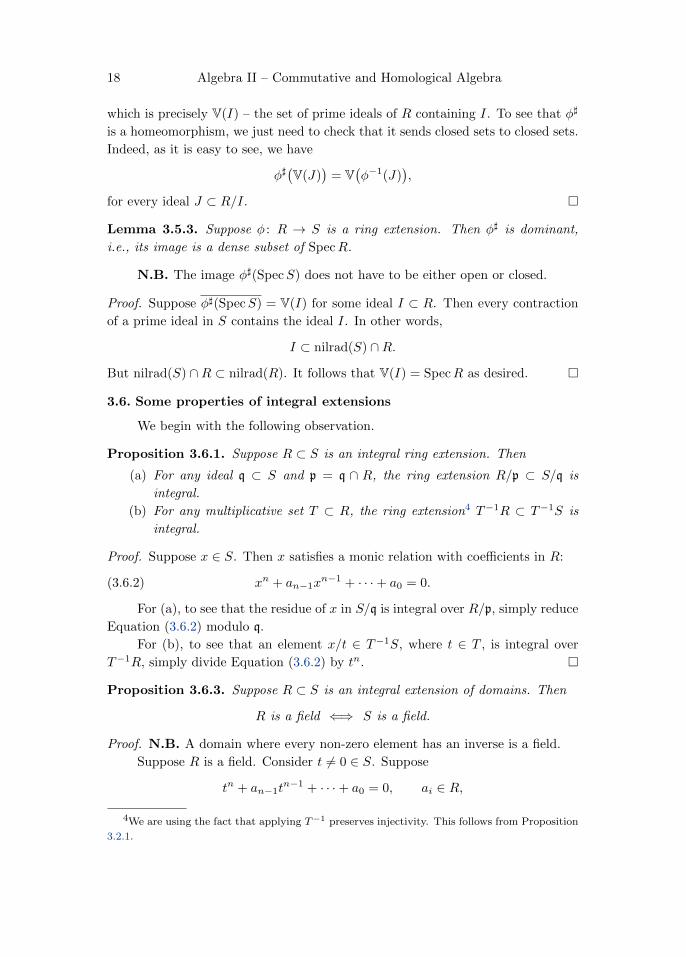
Lemma 3.5.3. Suppose φ : R → S is a ring extension. Then φ] is dominant,

i.e., its image is a dense subset of SpecR.

N.B. The image φ](SpecS) does not have to be either open or closed.

Proof. Suppose φ](SpecS) = V(I) for some ideal I ⊂ R. Then every contraction

of a prime ideal in S contains the ideal I. In other words,

I ⊂ nilrad(S) ∩R.

But nilrad(S) ∩R ⊂ nilrad(R). It follows that V(I) = SpecR as desired. �

3.6. Some properties of integral extensions

We begin with the following observation.

Proposition 3.6.1. Suppose R ⊂ S is an integral ring extension. Then

(a) For any ideal q ⊂ S and p = q ∩ R, the ring extension R/p ⊂ S/q is

integral.

(b) For any multiplicative set T ⊂ R, the ring extension4 T−1R ⊂ T−1S is

integral.

Proof. Suppose x ∈ S. Then x satisfies a monic relation with coefficients in R:

(3.6.2) xn + an−1xn−1 + · · ·+ a0 = 0.

For (a), to see that the residue of x in S/q is integral over R/p, simply reduce

Equation (3.6.2) modulo q.

For (b), to see that an element x/t ∈ T−1S, where t ∈ T , is integral over

T−1R, simply divide Equation (3.6.2) by tn. �

Proposition 3.6.3. Suppose R ⊂ S is an integral extension of domains. Then

R is a field ⇐⇒ S is a field.

Proof. N.B. A domain where every non-zero element has an inverse is a field.

Suppose R is a field. Consider t 6= 0 ∈ S. Suppose

tn + an−1tn−1 + · · ·+ a0 = 0, ai ∈ R,

4We are using the fact that applying T−1 preserves injectivity. This follows from Proposition

3.2.1.


is an integral dependence relation on t of the smallest possible degree. Because S

is a domain, we must have a0 6= 0. Clearly, then t has a multiplicative inverse in

S:

t−1 = − 1

a0(tn−1 + an−1t

n−2 + · · ·+ a1).

Suppose S is a field. Then for x 6= 0 ∈ R, we have x−1 ∈ S. Suppose

(x−1)n + bn−1(x−1)n−1 + · · ·+ b0 = 0, bi ∈ R,

is an integral dependence relation satisfied by x−1. It is now easy to see that

x−1 ∈ R:

x−1 = −(b0xn−1 + b1x

n−2 + · · ·+ bn−1).

�

Corollary 3.6.4. Suppose R ⊂ S is an integral ring extension. Let q ⊂ S be a

prime ideal and p = q ∩R. Then

q is maximal ⇐⇒ p is maximal.

Proof. Passing to the quotients and using Proposition 3.6.1(a), we get an integral

extension of integral domains

R/p ⊂ S/q.

The claim follows by Proposition 3.6.3. �

Example 3.6.5.

(1) Consider k[x] ⊂ k[x, y] and a prime non-maximal ideal q = (x − a) ⊂k[x, y]. The contracted ideal q ∩ k[x] = (x− a) ⊂ k[x] is maximal.

(2) Consider k[x, y] → k[x, y]p, where with p = (f) ⊂ k[x, y] is a prime non-

maximal ideal generated by an irreducible polynomial f . Then the max-

imal ideal pk[x, y]p in the local ring contracts to a non-maximal ideal

p ⊂ k[x, y].

(3) Consider R ⊂ Frac(R), where R is a PID (e.g., R = Z). The maximal

ideal (0) ⊂ Frac(R) contracts to a non-maximal prime ideal (0) ⊂ R.

3.7. Cohen-Seidenberg Theorems

Theorem 3.7.1 (Lying Over). Suppose R ⊂ S is an integral ring extension and

p ∈ SpecR. Then there exists q ∈ SpecS such that p = q ∩R.

N.B. In other words, this theorem says that when S is integral over R, the

inclusion R ⊂ S induces a surjective map (see Section 2.2) of sets SpecS → SpecR.

Proof. Let T = R \ p. By Proposition 3.6.1(b), the extension Rp ⊂ T−1S is

integral. Take m ⊂ T−1S to be any maximal ideal. Then by Corollary 3.6.4, the

ideal m∩Rp is maximal and hence equals to the unique maximal ideal of the local


ring Rp. We conclude that m ∩R = (m ∩Rp) ∩R = pRp ∩R = p. Set q = m ∩ S.

Then q is a prime ideal in S, and we have

q ∩R = (m ∩ S) ∩R = m ∩R = p.

�

Example 3.7.2. The homomorphism Z → Z(p) is not integral and SpecZ(p) →SpecZ is clearly not surjective as the image consists of only two elements: the

prime ideals (p) and (0).

Theorem 3.7.3 (Going Up). Suppose R ⊂ S is an integral ring extension. Let

p1 ⊂ · · · ⊂ pn

be a chain of prime ideals in R and

q1 ⊂ · · · ⊂ qm(†)

be a chain of prime ideals in S (with m < n) such that pi = qi∩R for i = 1, . . . ,m.

Then there is an extension of (†)

q1 ⊂ · · · ⊂ qn

such that pi = qi ∩R for i = 1, . . . , n.

Proof. Clearly, it suffices to establish the case of n = 2 and m = 1.

Let R = R/p1 and S = S/q1. Then R ⊂ S is an integral extension of domains

by Proposition 3.6.1(a). The prime ideal p2 in R gives rise to a prime ideal p2 in

R. By Theorem 3.7.1, there is a prime q ⊂ S such that q∩R = p2. Set q2 := q∩S.

Then q2 is a prime containing q1 and such that q2 ∩R = p2. �

Definition 3.7.4 (Integral closure of an ideal). Suppose R ⊂ S is an extension

of rings. We say that x ∈ S is integral over an ideal I ⊂ R if x satisfies

xn + an−1xn−1 + · · ·+ a0 = 0,

where ai ∈ I. The integral closure of I in S is the set of all elements in S

integral over I.

In particular, the integral closure of R in S is the set of all elements in S

integral over R. The integral closure of R in S is a ring by Proposition 1.1.4. We

say that R is integrally closed in S if its integral closure in S is just R. The

following result describes the structure of the integral closure in S of an arbitrary

ideal I ⊂ R.

Lemma 3.7.5. Suppose R ⊂ S is an extension of rings and let C be the integral

closure of R in S. For an ideal I ⊂ R, let Ie = IC ⊂ C be the extension of I to

C. Then the integral closure of I in S is rad(Ie) ⊂ C.


Proof. Suppose x ∈ S is integral over I. Then in particular x is integral over R

and so x ∈ C. We have

xn + an−1xn−1 + · · ·+ a0 = 0,

for some ai ∈ I. Then xn = −(an−1xn−1+· · ·+a0) ∈ IC = Ie. Hence x ∈ rad(Ie).

Conversely, suppose x ∈ rad(Ie). Then

xd =

m∑i=1

aixi,

for some d, some a1, . . . , am ∈ I, and some x1, . . . , xm ∈ C. Since each xi is integral

over R, the ring M := A[x1, . . . , xm] is a finitely generated A-module. Since

xd ∈M , the multiplication by xd defines an A-module endomorphism φ : M →M ,

given by φ(a) = xda. Since xd =∑mi=1 aixi ∈ IM , we have φ(M) ⊂ IM . It follows

by the Cayley-Hamilton Theorem 1.1.2 that

φn + cn−1φn−1 + · · ·+ c0 = 0

for some cn−1, . . . , c0 ∈ I. In particular, applying the above endomorphism to

1 ∈M , we obtain

xnd + cn−1x(n−1)d + · · ·+ c0 = 0,

which proves that x is integral over I. �

Definition 3.7.6. An integral domain is normal if it is integrally closed in its

field of fractions.

Lemma 3.7.7. Suppose R ⊂ S is an integral extension of domains with R inte-

grally closed in K := Frac(R) (that is, R is normal). Suppose x ∈ S is integral

over an ideal I ⊂ R. Then x (considered as an element of the field L := Frac(S)) is

algebraic over K and its minimal monic polynomial P (t) = tn+an−1tn−1 +· · ·+a0

over K satisfies ai ∈ rad(I).

Proof. Clearly, L is algebraic over K. Suppose x ∈ S is integral over an ideal I.

Then x satisfies a monic polynomial relation with coefficients in I:

f(x) = xm + cm−1xm−1 + · · ·+ c0 = 0.

Let x1, x2, . . . , xm be the roots of f(x) in some algebraic closure L of the field L.

Then each xi ∈ L is integral over I ⊂ R. Let P (t) = tn + an−1tn−1 + · · · + a0

be the minimal monic polynomial for x ∈ L over K. Then because f(x) = 0, we

must have P (t) | f(t). Hence the roots of P (t) in L are among {x1, x2, . . . , xm}. It

follows that the coefficients of P (t) are polynomials in xi’s and so are also integral

over I. (Recall that the integral closure of I in L is closed under addition and

multiplication by Lemma 3.7.5.) But the coefficients of P (t) are in K = Frac(R)

and R is integrally closed in K by the normality assumption. It follows that

a0, . . . , an−1 ∈ R. By Lemma 3.7.5 (applied to the ring extension R ⊂ Frac(R))

we conclude that ai ∈ rad(I). �


Theorem 3.7.8 (Going Down). Suppose that R is a normal ring (integrally closed

in its field of fractions) and R ⊂ S is an integral ring extension of domains. Let

p1 ⊃ · · · ⊃ pn

be a chain of prime ideals in R and

q1 ⊃ · · · ⊃ qm(‡)

be a chain of prime ideals in S (with m < n) such that pi = qi∩R for i = 1, . . . ,m.

Then there is an extension of (‡)

q1 ⊃ · · · ⊃ qn

such that pi = qi ∩R for i = 1, . . . , n.

Proof. Clearly, it suffices to prove the statement for n = 2 and m = 1.

So suppose p1 ⊃ p2 are prime ideals in R and q1 is a prime ideal in S such

that q1 ∩R = p1. Our goal is to find a prime q2 ⊂ q1 such that q2 ∩R = p2. Since

primes of S contained in q1 are in one-to-one correspondence with primes of the

local ring Sq1 , we pass to the ring extension R ⊂ Sq1 . (Note that we have used

here the fact that S ⊂ Sq1is an extension of domains.) It will now suffice to prove

an existence of a prime ideal in Sq1which contracts to p2 in R. By Proposition

3.4.5, it suffices to show that

p2Sq1∩R = p2.

Suppose x ∈ p2Sq1 . Then we can write

x =y

z, where y ∈ p2S and z ∈ S \ q1.

By Lemma 3.7.5 (applied to the extension R ⊂ S), the element y ∈ S is integral

over the ideal p2. By Lemma 3.7.7, the minimal monic polynomial for y over

K = Frac(R) is of the form

(3.7.9) yr + u1yr−1 + · · ·+ ur = 0, where ui ∈ p2.

Suppose now x =y

z∈ p2Sq1

∩R. Then z = yx−1 and since x−1 ∈ K, the minimal

polynomial for z over K is obtained by dividing (3.7.9) by xr:

(3.7.10) zr + v1zr−1 + · · ·+ vr = 0, where vi =

uixi.

Since z ∈ S \ q1 is integral over R, we conclude by Lemma 3.7.7 (applied with

I = R) that v1, . . . , vr ∈ R.

Note that xivi = ui ∈ p2. Suppose by way of contradiction that x /∈ p2.

Then vi ∈ p2 and so by Equation (3.7.10)

zr = −v1zr−1 − · · · − vr ∈ p2S ⊂ p1S ⊂ q1.

This shows that z ∈ q1. A contradiction!

�


Lemma 3.7.11. Suppose R ⊂ S is an extension of rings with R being a domain.

Then (0) ⊂ R is a contraction of a prime ideal in S.


Example 3.7.12. Here we give an example which illustrates how the Going-Down

Theorem can fail when R is not assumed to be normal. We take

R = k[x, y, z, w]/(w2(x+1)−z2, wx(x+1)−yz, xz−wy, y2−x2(x+1)) and S = k[a, t].

Consider the ring homomorphism

φ : R→ S

x 7→ t2 − 1

y 7→ t3 − tz 7→ at

w 7→ a.

By Problem Set 3, φ is an injection. Clearly, S is integral over R. In fact, S is an

integral closure of R in FracR = FracS = k(a, t). So we are in the situation of

Theorem 3.7.8 with the exception that R is not normal.

Let p1 = (x, y, z, w) ⊃ p2 = (x, y, z−w) and q1 = (a, t+1). Then q1∩R = p1.

Claim 3.7.13. There is no prime q2 ⊂ q1 such that q2 ∩R = p2.

Proof of Claim: S/p2S = k[a, t]/(t2 − 1, t3 − t, at − t) = k[a, t]/(t2 − 1, a(t − 1)).

It follows that the minimal primes of S/p2S are (t − 1) and (a, t + 1). However,

(a, t+ 1) = q1 and (t− 1) * q1. �

Lemma 3.7.14. Suppose R ⊂ S is an integral extension of domains. Then for a

prime ideal q ⊂ S,

q ∩R = (0) =⇒ q = (0).

Proof. Take b ∈ q and consider a monic relation of minimal degree with coefficients

in R satisfied by b:

bn + an−1bn−1 + · · ·+ a0 = 0.

Clearly, a0 ∈ q ∩ R = (0). Therefore, a0 = 0 and by minimality we conclude that

n = 1 and b = 0. �

Proposition 3.7.15 (Incomparability). Suppose R ⊂ S is an integral extension

of rings. If q1 ⊂ q2 are primes ideals in S with

q1 ∩R = q2 ∩R = p,

then q1 = q2.

Proof. R/p ⊂ S/q1 is an an integral extension by Proposition 3.6.1 (a) and q2 is

a prime ideal in S/q1 satisfying q2 ∩ R/p = 0. By Lemma 3.7.14, q2 = 0. So

q1 = q2. �


4. Grobner bases

In Example 3.7.12, the ideal I = (w2(x + 1) − z2, wx(x + 1) − yz, xz −wy, y2 − x2(x+ 1)) is precisely the ideal of all possible algebraic relations among

the elements x = t2 − 1, y = t3 − t, z = at and w = a in the polynomial ring

k[a, t]. However, to prove this rigorously, some work is required (cf. Problem Set

3). In this section, we discuss a general algorithmic procedure for finding algebraic

relations among elements of a polynomial ring.

Throughout this section, we take k to be a field.

4.1. Elimination problem

Suppose f1, . . . , fr ∈ k[y1, . . . , ys] are polynomials in variables y1, . . . , ys. We

say that f1, . . . , fr are algebraically dependent if there exists a polynomial F ∈k[x1, . . . , xr] such that

(4.1.1) F (f1, . . . , fr) = 0.

An element F ∈ k[x1, . . . , xr] satisfying (4.1.1) is called an algebraic relation

among f1, . . . , fr. It is clear that the set of algebraic relations among f1, . . . , frforms an ideal in k[x1, . . . , xr]. It will be called the ideal of algebraic relations

among f1, . . . , fr.

Lemma 4.1.2. The ideal of algebraic relations among f1, . . . , fr ∈ k[y1, . . . , ys] is

given by the ideal

(x1 − f1, . . . , xr − fr) ∩ k[x1, . . . , xr].

Proof. By definition, the ideal of algebraic relations among f1, . . . , fr ∈ k[y1, . . . , ys]

is the kernel of the ring homomorphism φ : k[x1, . . . , xr] → k[y1, . . . , ys] given by

φ(xi) = fi. Let Φ: k[x1, . . . , xr, y1, . . . , ys] → k[y1, . . . , ys] be a ring homomor-

phism given by Φ(xi) = fi and Φ(yj) = yj . Then ker(Φ) = (x1 − f1, . . . , xr −fr). The claim follows from the fact φ is a composition of Φ with the inclusion

k[x1, . . . , xr] ↪→ k[x1, . . . , xr, y1, . . . , ys]. �

Example 4.1.3. The three polynomials f1 = y21 , f2 = y1y2, f3 = y2

2 are alge-

braically dependent because they satisfy

f1f3 = f22 .

In fact, x1x3 − x22 generates the ideal of algebraic relations among f1, f2, f3. To

see this note that any algebraic relation among f1, f2, f3 can be written modulo

x1x3 − x22 as F (x1, x3)− x2G(x1, x3). We then must have

F (y21 , y

23) = y1y2G(y2

1 , y23).

However, every monomial on the left is even in each of the variables y1 and y3,

while every monomial on the right is odd in each of the variables y1 and y3. This

shows that F = G = 0 and the claim follows.


5. Dimension Theory

5.1. Nakayama’s lemma

Recall that the Jacobson radical of a ring R is the intersection of all max-

imal ideals of R. Clearly, the Jacobson radical of a local ring R is simply the

maximal ideal of R.

Theorem 5.1.1 (Nakayama’s lemma). Let R be a ring and M a finitely generated

R-module. Suppose that an ideal I is contained in the Jacobson radical of R. Then

(1) If IM = M , then M = 0.

(2) If images of elements m1, . . . ,mr generate M/IM as an R/I-module, then

m1, . . . ,mr generated M as an R-module.

Proof. The fact that IM = M implies by the Cayley-Hamilton theorem that there

exists x ≡ 1 (mod I) such that xM = 0 (see Corollary 1.1.3). However, such x is

a unit by Lemma 5.1.2 below. It follows that M = 0.

The second part follows by noting that N = M/(m1R+ · · ·+mrR) satisfies

N = IN since every element of M can be written as a linear combination of

m1, . . . ,mr modulo IM . Namely, the following sequence is exact:

0 = M/(IM + (m1R+ · · ·+mrR))→ N/IN → 0.

�

Lemma 5.1.2. Let R be a ring. Suppose x ≡ 1 modulo the Jacobson radical of

R. Then x is a unit.

Proof. Suppose not. Then x ∈ m for some maximal ideal m. This contradicts the

fact that x ≡ 1 (mod m). �

5.2. Artinian rings

Recall that a ring R is Artinian if it satisfies the descending chain condition

(DCC) on ideals, and if and only if every set of ideals in R has a minimal element.

Lemma 5.2.1. Let R be a Noetherian ring. Suppose m1, . . . ,mr are maximal

ideals such that m1 · · ·mr = (0). Then R is Artinian.

Proof. Consider a filtration of R by the ideals (i.e., R-submodules)Mi :=∏ij=1 mj ,

for i = 1, . . . , r:

(0) = Mr ⊂Mr−1 ⊂ · · · ⊂M1 ⊂M0 := M.

Each Mi, being an ideal in a Noetherian ring R, is a Noetherian R-module. Then

Mi/Mi+1 is Noetherian (by Lemma 1.2.8) and so is a finitely generated R-module.

Clearly, Mi/Mi+1 is annihilated by mi+1. Thus Mi/Mi+1 is a finitely generated

R/mi+1-module, hence a finite-dimensional R/mi+1-vector space. As such, it is

also an Artinian R/mi+1-module, hence Artinian R-module. Since every Mi/Mi+1


is an Artinian R-module, we conclude that each Mi is an Artinian R-module using

ascending induction on i and applying Lemma 1.2.8 to the exact sequence

0→Mi →Mi+1 →Mi/Mi+1.

�

Lemma 5.2.2. A Noetherian ring R in which every prime ideal is maximal is

Artinian.

Remark 5.2.3. In a ring, every prime ideal is maximal if and only if every chain5

of prime ideals has length 0 if and only if every prime ideal is a minimal prime.

Proof. Recall that every Noetherian ring has finitely many minimal prime ideals

by Proposition 1.3.9. Since every ideal of R is minimal by the assumption and

the above remark, it follows that R has finitely many primes. Let m1, . . . ,mk be

the (finitely many!) prime ideals of R. We have that m1 · · ·mk ⊂ m1 ∩ · · · ∩mk =

nilrad(R). Since R is Noetherian, the nilradical nilrad(R) is nilpotent (see Problem

1 on Problem Set 4). Hence (m1 · · ·mk)N = 0 for some N . Applying Lemma 5.2.1

(with r = kN) now gives the desired result. �

5.3. Krull dimension

Definition 5.3.1. The Krull dimension of a ring R is

dim(R) := sup{d | there exists a chain of prime ideals p0 ( p1 ( · · · ( pd}.

Example 5.3.2. If k is a field, then dim k = 0. If R is a PID, not a field, then

dimR = 1.

Definition 5.3.3. If I is an ideal of R, we define dim I := dim(R/I). The height

(or the codimension) of a prime ideal p ⊂ R is defined to be dimRp, so that

ht(p) := sup{d | there exists a chain of prime ideals p0 ( p1 ( · · · ( pd−1 ( p}.

We also define the height of an arbitrary ideal I to be the supremum of dimRp,

where p ranges over all minimal primes of I. It is denoted as codim I or as ht I.

Proposition 5.3.4. Let R be a ring. If R is Artinian, then dimR = 0. If R is

Noetherian and dimR = 0, then R is Artinian.

Proof. If R is Artinian and p is any prime ideal of R, then R/p is an Artinian

integral domain. Hence R/p by Problem 2 on Problem Set 4. That is, p is a

maximal ideal. We conclude that dimR = 0.

Now suppose that dimR = 0. Then every prime ideal is maximal. So R is

Artinian by Lemma 5.2.2. �

Scholium 5.3.5. An Artinian integral domain is a field, and vice versa.

5The length of a chain is the number of strict inclusions.


Remark 5.3.6. What goes wrong if R is not Noetherian? Consider the ring

R =∏∞i=1 k, where k is a field. Then dimR = 0, but R is not Artinian by

Problem Set 4.

Lemma 5.3.7. Let R be a ring. Then every minimal prime of R consists entirely

of zero-divisors.


Theorem 5.3.8 (Krull’s Principal Ideal Theorem). Let R be a Noetherian ring.

For any x ∈ R, we have codim(x) ≤ 1. In other words, any minimal prime p over

x has ht(p) ≤ 1. Moreover, if x is a non-zerodivisor, then ht(p) = 1.

Proof. Suppose first that x is a non-zerodivisor, then by Lemma 5.3.7, x does not

lie inside a minimal prime of (0). Hence, ht(p) ≥ 1.

After localizing at p, we can assume that R is local and p is a maximal ideal.

Suppose that q 6= p is a prime ideal of R. The goal is to show that ht(q) = 0, or,

equivalently, that Rq is Artinian. With this in mind, we consider φ : R→ Rq, set

n := qRq and define

q(k) := φ−1(nk).

Since the maximal ideal p is a minimal prime over x, the ring R/(x) has

only one prime ideal. By Lemma 5.2.2, R/(x) is Artinian and so satisfies DCC. It

follows that the descending chain of ideals

q(k) + (x) ⊃ q(k+1) + (x) ⊃ . . .

stabilizes in R. Say, q(n) + (x) = q(n+1) + (x). Then for any a ∈ q(n) we can write

a = b+ xc

where b ∈ q(n+1). It follows that φ(xc) ∈ nn. But φ(x) is a unit in Rq. Hence,

φ(c) ∈ nn and so c ∈ q(n). It follows that we have an equality of R-modules:

x · (q(n)/q(n+1)) = q(n)/q(n+1).

Since x is in the maximal ideal p, we conclude using Nakayama’s lemma in R that

q(n)/q(n+1) = 0, and so q(n) = q(n+1). Extending6 to Rq, we get nn = nn+1. By

Nakayama’s lemma in Rq, we conclude that nn = 0, and so Rq is Artinian by

Lemma 5.2.1.

�

Theorem 5.3.9 (Krull’s Height Theorem). Let R be a Noetherian ring and

x1, . . . , xc ∈ R. Then for any minimal prime p of (x1, . . . , xc) we have ht(p) ≤ c.

6The extension of any contraction is the original ideal by Proposition 3.4.1(1).


Proof. We proceed by induction. The case of c = 1 is Krull’s Principal Ideal

Theorem 5.3.8. After localizing at p, we can assume that p is a maximal ideal of

the local ring R. Let q 6= p be a prime ideal in R of the maximal possible height.

Since p is a minimal ideal over (x1, . . . , xc), we know that (x1, . . . , xc) * q. Say,

xc /∈ q. Then the ring R/(xc, q) has only one prime, hence is Artinian. (Indeed,

the only prime ideal containing q and xc is p.) It follows that for every element

xi, i = 1, . . . , c− 1, we can find ni ∈ N and an element yi ∈ q such that

yi = xnii mod xc.

The ideal p := p/(y1, . . . , yc−1) is then a minimal prime lying over xc in the ring

R/(y1, . . . , yc−1). It follows that ht(p) ≤ 1. It follows that for q := q/(y1, . . . , yc−1),

we have ht(q) = 0. It follows that q is a minimal prime of (y1, . . . , yc−1) in R. By

induction assumption, ht(q) ≤ c− 1. Hence, ht(p) ≤ c. �

Corollary 5.3.10. Prime ideals in a Noetherian ring satisfy DCC.

Proof. Let p = (f1, . . . , fc) be a prime ideal. Then by the previous theorem,

ht(p) ≤ c. It follows that every chain of prime ideals descending from p has length

at most c. �

Remark 5.3.11. Note that if a prime ideal p of height c is minimal over an ideal

I, then I is not necessarily generated by c elements. Indeed, in an Artinian ring

every prime has height 0.

Example 5.3.12. In the ring R = k[x, y, z]/(xy − z2), the prime ideal (x, z) has

height 1. Indeed, R(x,z) = k[y, z](z) is a PID. One easily checks that (x, z) is not

principal. Note, however, that (x, z) is a minimal prime of the principal ideal (x).

Lemma 5.3.13 (Prime avoidance). Let r be a positive integer. Suppose p1, . . . , prare prime ideals and I is an ideal such that

I ⊂r⋃i=1

pi.

Then there is an index i such that I ⊂ pi.

Proof. Homework exercise. �

The converse of Theorem 5.3.9 holds in the following sense.

Proposition 5.3.14 (Converse to the Krull’s Principal Ideal Theorem). Let R be

a Noetherian ring. If p is a prime of height c in R, then for every j ≤ c, there

exists Ij = (x1, . . . , xj) ⊂ p such that all minimal primes of Ij have height exactly

j. In particular, p is a minimal prime of the ideal Ic = (x1, . . . , xc).

Proof. Once Ic with the claimed property is constructed, p must be a minimal

prime of Ic because ht(p) = c and so cannot properly contain any minimal prime

of Ic.


To prove the existence of Ij , we argue by induction on j. Suppose j = 1.

Since p is not contained in the union of the finitely many minimal primes of R by

Prive Avoidance Lemma 5.3.13, we must have x1 ∈ p such that x1 is not contained

in any minimal prime of R. In particular, every minimal prime of (x1) has height

exactly 1 (N.B. x1 could still be a zero-divisor).

Suppose j ≤ c − 1 and Ij = (x1, . . . , xj) is an ideal inside p such that all

minimal prime ideals of Ij have height j. Since ht(p) = c ≥ j + 1, we know that

p is not a minimal prime ideal of Ij . By Prime Avoidance Lemma 5.3.13, there is

xj+1 ∈ p such that xj+1 is not contained in any minimal prime of Ij . Suppose q is

a minimal prime of Ij+1 = (x1, . . . , xj , xj+1). Since xj+1 ∈ q, Ij+1 must properly

contain some minimal prime of Ij . Therefore, ht(q) ≥ j + 1. By Krull’s Height

Theorem 5.3.9, ht(q) ≤ j + 1. We conclude that ht(q) = j + 1 as desired. �

algebra ii { commutative and homological algebra - bc.edu · pdf filealgebra ii { commutative...

Documents