Notes on Homological Algebra

Ieke MoerdijkUniversity of Utrecht

January 15, 2008

Contents

Foreword iii

1 Modules over a ring 11.1 Modules . . . . . . . . . . . . . . . . . . . . . . . . . . . . . . . . 11.2 The Hom Functor . . . . . . . . . . . . . . . . . . . . . . . . . . 31.3 Tensor Product . . . . . . . . . . . . . . . . . . . . . . . . . . . . 51.4 Adjoint Isomorphism . . . . . . . . . . . . . . . . . . . . . . . . . 71.5 Change of Ring . . . . . . . . . . . . . . . . . . . . . . . . . . . . 81.6 Exact Sequences . . . . . . . . . . . . . . . . . . . . . . . . . . . 91.7 Projective Modules . . . . . . . . . . . . . . . . . . . . . . . . . . 131.8 Injective Modules . . . . . . . . . . . . . . . . . . . . . . . . . . . 141.9 Complexes . . . . . . . . . . . . . . . . . . . . . . . . . . . . . . . 181.10 Homotopy of chain complexes . . . . . . . . . . . . . . . . . . . . 231.11 Double Complexes . . . . . . . . . . . . . . . . . . . . . . . . . . 271.12 The Kunneth formula . . . . . . . . . . . . . . . . . . . . . . . . 311.13 Additional exercises . . . . . . . . . . . . . . . . . . . . . . . . . 36

2 Cohomology of groups 372.1 Cohomology of a group . . . . . . . . . . . . . . . . . . . . . . . 372.2 Functoriality of cohomology . . . . . . . . . . . . . . . . . . . . . 40

2.2.1 Functoriality in A . . . . . . . . . . . . . . . . . . . . . . 402.2.2 Functoriality in G . . . . . . . . . . . . . . . . . . . . . . 41

2.3 Cohomology of cyclic groups . . . . . . . . . . . . . . . . . . . . 422.4 The bar resolution . . . . . . . . . . . . . . . . . . . . . . . . . . 432.5 Group extensions and H2 . . . . . . . . . . . . . . . . . . . . . . 482.6 Additional exercises . . . . . . . . . . . . . . . . . . . . . . . . . 54

3 Chain complexes in algebraic topology 573.1 Simplicial methods . . . . . . . . . . . . . . . . . . . . . . . . . . 57

3.1.1 Simplicial homotopies . . . . . . . . . . . . . . . . . . . . 613.2 The Mayer-Vietoris sequence . . . . . . . . . . . . . . . . . . . . 633.3 The Eilenberg-Zilber isomorphism . . . . . . . . . . . . . . . . . 713.4 Additional exercises . . . . . . . . . . . . . . . . . . . . . . . . . 77

4 Abelian categories and derived functors 794.1 Abelian categories . . . . . . . . . . . . . . . . . . . . . . . . . . 794.2 Derived functors . . . . . . . . . . . . . . . . . . . . . . . . . . . 87

4.2.1 Left derived functors . . . . . . . . . . . . . . . . . . . . . 88

i

4.2.2 Right derived functors . . . . . . . . . . . . . . . . . . . . 924.3 Cohomology of Small Categories . . . . . . . . . . . . . . . . . . 95

4.3.1 The nerve of a category . . . . . . . . . . . . . . . . . . . 984.4 Sheaf cohomology . . . . . . . . . . . . . . . . . . . . . . . . . . . 100

4.4.1 Germs of functions . . . . . . . . . . . . . . . . . . . . . . 1014.5 Additional exercises . . . . . . . . . . . . . . . . . . . . . . . . . 104

A Categories and Functors 106

Bibliography 112

ii

Foreword

These are the notes of a course I taught in Utrecht in the fall of 2003, in thecontext of the Master Class on Non-Commutative Geometry, a one year specialprogramme for a group of around 15 students from many different countries.The material is a selection of standard results which can be found in many ofthe text books on the subject, e.g. the one by C. Weibel (Cambridge UniversityPress) or the one by P. Hilton and U. Stammbach (Springer-Verlag). A firstdraft of the notes was prepared by these students. Subsequently, the notes werepolished with the help of Federico De Marchi, who also added an appendixon categorical language. Later, Roald Koudenburg added two sections on theKunneth formula and the Eilenberg-Zilber isomorphism. I’d like to take thisopportunity to express my thanks to the students of the Master Class for beingan enthusiastic audience, and to Federico, Roald and these students for all theirwork on the notes.

Utrecht,April 2005 and September 2007I. Moerdijk

1. Modules over a ring

By a ring, in this course, we intend an abelian group (in additive notation) witha product operation, which distributes over the sum, is associative and has aunit 1 6= 0.

The most standard examples of such a structure are the (commutative) ringZ of integer numbers, the fields Q, R and C of rational, real and complexnumbers, respectively, and the group ring Z[G] (see Chapter 2, Definition 2.1.1),which is not necessarily commutative.

1.1 Modules

Modules play to rings the same role as vector spaces do with respect to fields.

Definition 1.1.1 A left R-module is an abelian group (A,+) equipped with anaction by R:

R×A 3 (r, a) 7→ r · a ∈ Asatisfying the following conditions:

a) r · (a+ b) = r · a+ r · b;b) r · 0 = 0;c) (r + s) · a = r · a+ s · a;d) r · (s · a) = (rs) · a;e) 1 · a = a.

Typically, when the action R×A //A is fixed in the context, we will write rainstead of r · a.

Example 1.1.2 The following is a list of basic examples of modules:

a) Every vector space over a field k is a k-module;b) Every abelian group is a Z-module;c) Every ring R is a module over itself, by taking as action R × R //R themultiplication of R.

Definition 1.1.3 Let A and B be left R-modules. A mapping φ:A //B iscalled an R-homomorphism if, for all a, a′ ∈ A and r ∈ R, we have:

φ(a+ a′) = φ(a) + φ(a′),φ(ra) = r · φ(a).

1

The composite of two R-homomorphisms is again an R-homomorphism, andthe identity map on a module is always an R-homomorphism. So, R-modulesand R-homomorphisms form a category (see Definition A.0.1), which we shallcall the category of left R-modules and will denote by R-mod.

Remark 1.1.4 The category mod-R of right R-modules is defined similarly.Only, this time the action associates on the right of the elements.

If (R,+, ·) is a ring, its dual R is the ring with the same underlying group,but with reversed multiplication:

r ∗ s = s · r,

for r, s ∈ R. It is then a trivial observation that the categories R-mod andmod-R are isomorphic.

WhenR is a commutative ring, it coincides with its dual, hence the categoriesof left and right R-modules coincide (up to isomorphism), and their objects aresimply called R-modules.

Definition 1.1.5 Given two rings R and S, we say that A is an (R,S)-bimoduleif A is a left R-module and a right S-module, and the two actions associate asfollows:

(ra)s = r(as),

for all r ∈ R, a ∈ A, s ∈ S.Given two (R,S)-bimodules, we call (R,S)-homomorphism a map between

them which is simultaneously an R-homomorphism and an S-homomorphism.(R,S)-bimodules and (R,S)-homomorphisms form again a category, which weshall denote by R-mod-S.

Example 1.1.6 In Example 1.1.2 c) above, R is an (R,R)-bimodule.

Let (Ai)i∈I be a family of left R-modules and let∏i∈I Ai be their cartesian

product as sets. Then, a typical element of∏i∈I Ai is a family (ai) with ai ∈ Ai

for all i ∈ I and (ai) = (a′i) if and only if ai = a′i for each i ∈ I. If (ai) and (a′i)are elements of

∏i∈I Ai and r ∈ R we set:

(ai) + (a′i) = (ai + a′i),r(ai) = (rai).

With these operations,∏i∈I Ai becomes a left R-module, called the direct

product of the family (Ai)i∈I . We call πj :∏i∈I Ai //Aj the j-th canonical

projection. The direct product of a family (Ai)i∈I is uniquely characterised(up to isomorphism) by the following universal property, which we leave you tocheck for yourself.

Proposition 1.1.7 For any left R-module B and any family (gi:B //Ai)i∈Iof R-homomorphisms, there exists a unique R-homomorphism g:B //

∏i∈I Ai

such that πi g = gi for all i ∈ I.

The subset of∏i∈I Ai consisting of those families (ai) with finitely many

non-zero elements ai clearly inherits the structure of an R-module. It is calledthe direct sum of the family (Ai)i∈I , and we shall denote it by

⊕i∈I Ai. For any j

2

in I there is an obvious map σj :Aj //⊕

i∈I Ai taking a ∈ Aj to the family (ai),with ai = 0 for i 6= j and aj = a. We call this map the j-th canonical injection.The direct sum of a family of left R-modules is again uniquely characterised (upto homomorphism) by a universal property, which again you should check foryourself.

Proposition 1.1.8 For any family (fi:Ai //B)i∈I of R-homomorphisms withcommon codomain B, there exists a unique R-homomorphism f :

⊕i∈I Ai //B

such that f σi = fi for all i ∈ I.Remark 1.1.9 Note that, when I is a finite set 1, ..., n, the R-modules∏i∈I Ai and

⊕i∈I Ai do coincide. In this case, we shall denote the resulting

module by A1 ⊕ · · · ⊕An.Definition 1.1.10 An R-module F is called free if it is isomorphic to a directsum of copies of R; that is, if there is a (possible infinite) index set I with:

F =⊕

i∈IRi

where Ri ' R for all i.

Note that, for a field k, every k-module is free.

1.2 The Hom Functor

Let A and B be two left R-modules. We can define on the set HomR-mod(A,B)of R-homomorphisms from A to B a sum operation, by setting

(φ+ ψ)(a) = φ(a) + ψ(a).

This gives the set the structure of an abelian group, which we denote byHomR(A,B).

Remark 1.2.1 Notice that there is a subtle but essential difference betweenHomR-mod(A,B) and HomR(A,B): their underlying set is the same, but thelatter has much more structure than the former. In particular, they live intwo different categories, namely Set and Ab (for definitions, see the Appendix,Example A.0.2).

Proposition 1.2.2 Just like the hom-sets give rise to Set-valued functors (seeDefinition A.0.6 and Example A.0.10), the HomR-groups determine Ab-valuedfunctors:

a) For a fixed R-module A, the assignment B 7→ HomR(A,B) defines acovariant functor HomR(A,−):R-mod //Ab;b) Analogously, for a fixed R module B, HomR(−, B) is a contravariantfunctor from R-mod to Ab.

Remark 1.2.3 Suppose R is a commutative ring. Then, we define an actionof R on the left of HomR(A,B) as follows:

(r · φ)(a) = r · (φ(a)),

3

for r ∈ R, φ ∈ HomR(A,B) and a ∈ A. This determines on HomR(A,B) thestructure of a left R-module.

Notice that, in this case, HomR(A,−) and HomR(−, B) can be seen as func-tors from the category R-mod to itself. Indeed, assume that A, A′, A′′ and Bare left R-modules and let φ:A′ //A be an R-homomorphism. Then, φ definesby precomposition an R-homomorphism

φ∗: HomR(A,B) // HomR(A′, B);

moreover, if ψ:A′′ //A′ is another R-homomorphism, then we have the equalityψ∗ φ∗ = (φ ψ)∗ of R-homomorphisms from HomR(A,B) to HomR(A′′, B).

Analogously, for left R-modules A, B, B′ and B′′, any R-homomorphismφ:B //B′ determines by composition an R-homomorphism

φ∗: HomR(A,B) // HomR(A,B′)

and, for a second map ψ:B′ //B′′, we have the equality of R-homomorphismsψ∗ φ∗ = (ψ φ)∗: HomR(A,B) // HomR(A,B′′).

Remark 1.2.4 Let R and S be two rings, and A and B two abelian groups.Then, the functor Hom relates different categories, depending on the way R andS act on A and B.

a) Let A be a left S-module and B an (S,R)-bimodule. In this situation, theabelian group HomS(A,B) can be endowed the structure of a right R-module,the action of r ∈ R on φ ∈ HomS(A,B) being given by φ · r:A //B defined as:

(φ · r)(a) = φ(a)r.

It follows that HomS(A,−) is a covariant functor from S-mod-R to mod-R andHomS(−, B) is a contravariant functor from S-mod to mod-R;b) If A is an (S,R)-bimodule and B is a right R-module, then HomR(A,B) isa right S-module with:

(φ · s)(a) = φ(sa),

thus determining the following functors: HomR(A,−): mod-R //mod-S andHomR(−, B):S-mod-R //mod-S;c) If A is a right R-module and B is an (S,R)-bimodule, then HomR(A,B) isa left S-module with:

(sφ)(a) = sφ(a),

thus determining the following functors: HomR(A,−):S-mod-R //S-mod andHomR(−, B): mod-R //S-mod;d) If A is an (S,R)-bimodule and B is a left S-module, then HomS(A,B) is aleft R-module with:

(rφ)(a) = φ(ar),

thus determining the following functors: HomS(A,−):S-mod //R-mod andHomS(−, B):S-mod-R //R-mod.

The universal properties of product and sums (Propositions 1.1.7 and 1.1.8)can now be refined as follows.

4

Proposition 1.2.5 Let A and B =∏j∈J Bj be left R-modules. Then, the map

(πj −): HomR(A,B) //∏

j∈JHomR(A,Bj)

taking a map φ to the family of composites (πj φ) is an isomorphism of abeliangroups. Moreover, if each Bi is an (R,S)-bimodule, then (πj −) is an isomor-phism of right S-modules.

Proposition 1.2.6 Let A =⊕

i∈I Ai and B be left R-modules. Then, the map

[− σi]: HomR(A,B) //∏

i∈IHomR(Ai, B)

taking a map φ to the family of composites (φσi) is an isomorphism of abeliangroups. Moreover, if each Ai is an (R,S)-bimodule, then this is actually anisomorphism of left S-modules.

Exercises

a) Recall from the Appendix Definition A.0.12; then show that the assign-ment φ 7→ φ∗ (resp. φ 7→ φ∗) of Remark 1.2.3 defines a natural trans-formation between the functors HomR(A,−) and HomR(A′,−) (resp.HomR(−, B) and HomR(−, B′)).

b) For a commutative ring R, consider the category End(R-mod), whose ob-jects are functors from R-mod to itself and morphisms are natural trans-formations between them. Using the previous exercise and Remark 1.2.3,show that the assignments A 7→ HomR(A,−) and B 7→ HomR(−, B) de-fine respectively a contravariant and a covariant functor from R-mod toEnd(R-mod).

c) Check that any R-module A is isomorphic to HomR(R,A).

1.3 Tensor Product

When working with modules, one can choose between two different product op-erations. One is the obvious cartesian product, which we have already examinedin Proposition 1.1.7; the other one, which will be essential for us, is called thetensor product.

Let A be a right R-module and B a left one. Then, we can build the freeabelian group F over their cartesian product A×B. Its elements can be uniquelywritten as finite sums ∑

i,j

pij(ai, bj),

for pij ∈ Z, ai ∈ A and bj ∈ B.Let now T be the subgroup of F generated by all elements of the form

(a+ a′, b)− (a, b)− (a′, b), (a, b+ b′)− (a, b)− (a, b′), (a, rb)− (ar, b)

where a, a′ ∈ A, b, b′ ∈ B and r ∈ R.

5

Definition 1.3.1 The quotient F/T has an obvious abelian group structure.We denote it by

A⊗R B,and we call it the tensor product of A and B.

The image of a pair (a, b) under the projection F //A⊗R B is denoted bya⊗b. With this notation, A⊗RB consists of all finite sums

∑i ai⊗bi, satisfying

the relations:

(a+ a′)⊗ b = a⊗ b+ a′ ⊗ ba⊗ (b+ b′) = a⊗ b+ a⊗ b′

a⊗ rb = ar ⊗ b.

The map f :A×B //A ⊗R B defined by f(a, b) = a ⊗ b is bilinear, i.e. itsatisfies the following properties:

a) f(a+ a′, b) = f(a, b) + f(a′, b);b) f(a, b+ b′) = f(a, b) + f(a, b′);c) f(ar, b) = f(a, rb).

These properties characterise the tensor product uniquely, up to isomorphism.In fact, you should check that the following universal property holds for tensorproducts:

Proposition 1.3.2 If C is an abelian group and φ:A×B //C is any bilinearmap, then there is a unique group homomorphism φ:A⊗R B //C making thefollowing diagram commute:

A×B f//

φ**

A⊗R Bφ

²²

C.

(1.1)

Example 1.3.3 Let φ:A //A′ and ψ:B //B′ be homomorphisms of rightand left R-modules, respectively. Then, the map γ:A×B //A′ ⊗R B′ definedby

γ(a, b) = φ(a)⊗ ψ(b)

is clearly bilinear, hence it induces a (unique!) homomorphism of abelian groups,γ:A⊗RB //A′⊗RB′, making (1.1) commute, i.e. such that for all (a, b) ∈ A×B

γ(a⊗ b) = φ(a)⊗ ψ(b).

We shall call γ the tensor product of φ and ψ, and we shall denote it by φ⊗ ψ.

In particular, when φ = idA, an R-homomorphism ψ:B //B′ induces ahomomorphism of abelian groups idA ⊗ ψ:A⊗R B //A⊗R B′, and similarly,when ψ = idB , every φ:A //A′ induces a map φ⊗ idB :A⊗R B //A′ ⊗R B.

Proposition 1.3.4 With the action on maps defined above, A⊗R− and −⊗RBdetermine covariant functors from R-mod to Ab and mod-R to Ab, respectively.

6

When either A or B have the structure of a bimodule, we can endow theabelian group A⊗R B with the structure of a module, as follows.

Let R and S be two rings, and assume that A is an (S,R)-bimodule andB is a left R-module. For each s ∈ S, the map φs:A×B //A ⊗R B definedby φs(a, b) = sa ⊗ b is easily shown to be bilinear; hence, it determines ahomomorphism φs:A⊗RB //A⊗RB such that φs(a⊗ b) = sa⊗ b for any pair(a, b) ∈ A×B.

We now define an action of S on A⊗R B by setting

s(a⊗ b) = φs(a⊗ b) = sa⊗ b.It is straightforward to check that, under this action, A ⊗R B becomes a leftS-module. Accordingly, A ⊗R − and − ⊗R B become covariant functors fromR-mod to S-mod and from S-mod-R to S-mod, respectively.

Analogously, when B is an (R,S)-bimodule and A is a right R-module,A⊗R B can be regarded as a right S-module by putting:

(a⊗ b)s = a⊗ bs.In this case, A⊗R− and −⊗RB will become covariant functors from R-mod-Sto mod-S and from mod-R to mod-S, respectively.

Finally, we observe that the universal properties of sum and tensor can beused to check the following:

Proposition 1.3.5 Let A =⊕

i∈I Ai and B =⊕

j∈J Bj be direct sums of rightR-modules and left R-modules, respectively. Then, there exists an isomorphismof abelian groups

A⊗R B '⊕

(i,j)∈I×J(Ai ⊗R Bj).

Exercise

a) Show that two integer numbers n and m are relatively prime if and onlyif Z/n⊗Z Z/m = 0.

1.4 Adjoint Isomorphism

Let R and S be two rings, A a right R-module, C a right S-module and B an(R,S)-bimodule. Then, with the notation introduced in the previous sections,we may form the groups HomS(A⊗RB,C) and HomR(A,HomS(B,C)). Theseare related as follows.

Theorem 1.4.1 The map

τA,C : HomS(A⊗R B,C) // HomR(A,HomS(B,C)) (1.2)

which takes an S-homomorphism α:A ⊗R B //C to the R-homomorphismα′:A // HomS(B,C) defined by

α′(a)(b) = α(a⊗ b)is an isomorphism of abelian groups.

7

Proof. It is clear that the given map is a group homomorphism. To defineits inverse, let β:A // HomS(B,C) be an R-homomorphism. Then, the mapA×B //C defined by (a, b) 7→ β(a)(b) is clearly bilinear. Hence, there exists agroup homomorphism ψ(β):A⊗R B //C such that

ψ(β)(a⊗ b) = β(a)(b).

Since β(a) is an S-homomorphism, so is ψ(β), and the assignment β 7→ ψ(β)defines a homomorphism of abelian groups, which is easily checked to be theinverse of τA,C . ¤

Exercises

a) Recall from the Appendix Definition A.0.16. Then, using Remark 1.2.1and Theorem 1.4.1, show that, for an (R,S)-bimodule B, the functor−⊗R B: mod-R //S-mod is left adjoint to the functor HomS(B,−).

b) State and prove a similar adjunction when Hom is taken to be one of thefunctors in Remark 1.2.4 a)− d).

1.5 Change of Ring

Let φ:R //S be a ring homomorphism. Then, for any left S-module A, theaction of S induces via φ an action of R on the left of A, defined by

r · a = φ(r)a.

If B is another left S-module and ψ ∈ HomS(A,B), then

ψ(r · a) = ψ(φ(r) · a) = φ(r)ψ(a) = r · ψ(a).

So, ψ can also be regarded as a member of HomR(A,B). In this way, φ definesa functor φ∗:S-mod //R-mod, or analogously from mod-S to mod-R.

In particular, by Example 1.1.2 c), we can regard S as an S-module, and φ∗

makes it into a right R-module, where the action is defined by s · r = sφ(r). Wehave that

(ss′) · r = (ss′)φ(r) = s(s′φ(r)) = s(s′ · r),thus giving S the structure of an (S,R)-bimodule, and we have the functor

φ! = S ⊗R −:R-mod //S-mod.

The action of φ! on an R-homomorphism τ :B //C gives the S-homomorphismφ!(τ) = idS ⊗ τ :S ⊗R B //S ⊗R C.

The functors φ∗ and φ! are related in the following way.

Theorem 1.5.1 There is an isomorphism of abelian groups

HomS(φ!(B), A) ' HomR(B,φ∗(A)), (1.3)

which is natural in A and B. In particular, the functor φ! is left adjoint to φ∗.

8

Proof. The proof is similar to that of Theorem 1.4.1, and we leave it as anexercise. (In fact, you can try to see it as an instance of one of the adjunctions inExercise 1.4–b), using the observation that φ∗(A) ∼= HomS(S,A) as R-modules.)

¤

Proposition 1.5.2 Let A =⊕

i∈I Ai be a left S-module. Then, there exists anisomorphism of R-modules

φ∗(A) '⊕

i∈Iφ∗(Ai).

Proposition 1.5.3 Let B =⊕

j∈J Bj be a left R-module. Then, there existsan isomorphism of S-modules

φ!(B) = S ⊗R B '⊕

j∈J(S ⊗R Bj) =

⊕

j∈Jφ!(Bj).

Proof. It follows immediately from Proposition 1.3.5. ¤

Finally, for a ring homomorphism φ as above, we can consider S as an(R,S)-bimodule (via φ) and define a third functor

φ∗ = HomR(S,−):R-mod //S-mod

as in Remark 1.2.4 d). Now, given a left S-module A and a left R-module B,we can compare the abelian groups HomR(φ∗A,B) and HomS(A,HomR(S,B)).Let α ∈ HomR(φ∗A,B) and let a ∈ A. Define ψa:S //B by ψa(s) = α(sa).Then, it is easy to check that the ψa’s are R-homomorphisms. Moreover,they satisfy the relations ψa+a′ = ψa + ψa′ and ψsa = sψa; hence, the mapα′:A // HomR(S,B) defined by α′(a) = ψa is an S-homomorphism from A toHomR(S,B). We now have a mapping

τA,B : HomR(φ∗(A), B) // HomS(A,HomR(S,B)),

defined by τA,B(α) = α′, which can easily be shown to be an isomorphism ofabelian groups. This gives a proof of the following.

Theorem 1.5.4 There is an isomorphism of abelian groups, natural in A andB:

HomR(φ∗(A), B) ' HomS(A,φ∗(B)).

In particular, the functor φ∗ is right adjoint to φ∗.

1.6 Exact Sequences

We now introduce the notions of kernel and cokernel of a module homomor-phism. Formally, they do not differ from the analogous notions for abeliangroups (after all, modules are abelian groups, with some extra structure). Infact, the isomorphism theorems do still hold in this setting, although in provingthem one has to verify the extra condition imposed by the action of the ring.So, let φ:A //B be an R-homomorphism.

9

Definition 1.6.1 The kernel of φ is the submodule ker(φ) of A defined as

ker(φ) = a ∈ A : φ(a) = 0;

the image of φ is the submodule im(φ) of B defined as

im(φ) = b ∈ B : there exists a ∈ A with φ(a) = b.

In particular, a submodule is a subgroup; hence, we can consider the quotientB/ im(φ) as abelian groups. It is easy to check that the action of R on B inducesone on the quotient; namely, r · a = r · a (where a is the equivalence class of a).We define the cokernel of φ to be the quotient module

coker(φ) = B/im(φ).

Definition 1.6.2 A (possibly infinite) sequence

· · · // Ai+1φi+1

// Aiφi // Ai−1

// · · · (1.4)

of R-modules and R-homomorphisms is exact at Ai if ker(φi) = im(φi+1). It isexact if it is exact at Ai for all i.

A short exact sequence is an exact sequence of the special form

0 // A′φ

// Aψ

// A′′ // 0. (1.5)

Example 1.6.3 The presence of 0’s in an exact sequence gives some informa-tion about the adjacent maps. Namely,

a) A sequence 0 //Aφ

//B is exact if and only if φ is injective;

b) A sequence Aψ

//B //0 is exact if and only if ψ is surjective.

Short exact sequences can be “composed”, and long ones decomposed, as in:

Proposition 1.6.4 (Splicing of exact sequences)

a) If the short sequences

0 // Aφ

// Bψ

// C // 0,

0 // Cα // D

β// E // 0

are exact, then there is a (long) exact sequence

0 // Aφ

// Bαψ

// Dβ

// E // 0.

b) Conversely, a long sequence as in (1.4) is exact at Ai if and only if thefollowing is a short exact sequence:

0 // im(φi+1) // Ai // im(φi) // 0.

10

The proof is left as an exercise at the end of this section.

Definition 1.6.5 Let A and B be R-modules, then A is a retract of B if thereexist R-homomorphisms s:A //B and r:B //A such that r s = idA. Whenthis happens, we say that s is a section of r, and r is a retraction of s.

Proposition 1.6.6 For a short exact sequence

0 // Af

// Cg

// B // 0

of left R-modules, the following are equivalent:

a) f has a retraction r:C //A;b) g has a section s:B //C;c) there is an isomorphism C ' A⊕B under which the short exact sequencerewrites as

0 // AσA // A⊕B πB // B // 0.

The proof is left as Exercise b) below.

Definition 1.6.7 We shall call split a short exact sequence satisfying the equiv-alent properties of Proposition 1.6.6.

Proposition 1.6.8 (5-lemma) In any commutative diagram

A′ //

a ∼=²²

B′ //

b ∼=²²

C ′ //

c

²²

D′ //

d ∼=²²

E′

e ∼=²²

A // B // C // D // E

with exact rows, if a, b, d and e are isomorphisms, then so is c. More precisely,if b and d are injective and a is surjective, then c is injective, and dually, if band d are surjective and e is injective, then c is surjective.

Proof. See Exercise c) below. ¤

Let C and D be categories of modules (or, more generally, categories in whichthe notion “exact sequence” is defined: see Chapter 4), and F :C //D a functorbetween them. In this case, it makes sense to ask whether F preserves exactnessof sequences.

Definition 1.6.9 F is said to be left exact if, whenever a short sequence as in(1.5) is exact in C, the following is exact in D:

0 //F (A′)Fφ

//F (A)Fψ

//F (A′′).

We say that F is right exact if, when (1.5) is exact, we have an exact sequence:

F (A′)Fφ

//F (A)Fψ

//F (A′′) //0.

Finally, F is said exact if it is both left exact and right exact, i.e. if it preservesthe exactness of short sequences (or equivalently, by Proposition 1.6.4, of longones).

11

Proposition 1.6.10 If a functor F : C //D between categories of modules isleft (respectively, right) exact, then it preserves monomorphisms (resp. epimor-phisms).

Remark 1.6.11 Bearing in mind that a contravariant functor F : C //D is justa covariant functor from Cop to D (see the Appendix for definitions), and thatclearly a short sequence is exact in C if and only if it is in Cop, one can easilystate the definition of left and right exactness for contravariant functors. It willthen follow that a left exact contravariant functor converts monomorphisms intoepimorphisms, and a right exact contravariant functor does the converse.

Next, we are going to analyse the exactness properties of the Hom and tensorproduct functors.

Proposition 1.6.12 Let B be a left R-module. Then, the contravariant functor

HomR(−, B):R-mod //Ab

is left exact.

Proof. Consider a short exact sequence of left R-modules as in (1.5). Then,we want to show the following sequence to be exact:

0 // HomR(A′′, B)ψ∗

// HomR(A,B)φ∗

// HomR(A′, B). (1.6)

To see that ψ∗ is injective, let f, g:A //B be two R-homomorphisms suchthat ψ∗(f) = ψ∗(g), i.e. fψ = gψ. Since (1.5) is exact, we know that ψ issurjective, therefore f = g, and the sequence (1.6) is exact at HomR(A′′, B).

For exactness at HomR(A,B), we need to show ker(φ∗) = im(ψ∗). ByRemark 1.2.3, φ∗ψ∗ = (ψφ)∗, but we know that ψφ is the null map, by theexactness of (1.5), hence φ∗ψ∗ = 0, and this shows that im(ψ∗) ⊂ ker(φ∗).

For the reverse inclusion, take a map f :A //B such that φ∗(f) = fφ = 0.We want to show that f = gψ for some g:A′ //B. Since fφ = 0, f factorsthrough the cokernel of φ, i.e. f = f ′π for some f ′, where π:A //A/ im(φ) isthe quotient projection. On the other hand, surjectivity of ψ determines an iso-morphism h:A′′ ' //A/ ker(ψ) = A/ im(φ), for which it holds hψ = π. Then,by taking g = f ′h we have f = f ′π = f ′hψ = gψ, and the result is proved. ¤

By analogous techniques, one proves the following.

Proposition 1.6.13 For a left R-module B, the functor

HomR(B,−):R-mod //Ab

is left exact.

Proposition 1.6.14 Let B be a left R-module. Then, the functor

−⊗R B: mod-R //Ab

is right exact.

12

Exercises

a) Prove Proposition 1.6.4.b) Prove Proposition 1.6.6.c) Prove Proposition 1.6.8.d) Recall from A.0.3 the definition of mono and epimorphisms; then, using

the characterisation of Example 1.6.3, give a proof of Proposition 1.6.10.e) Make precise and verify the claims of Remark 1.6.11.f) Prove Proposition 1.6.13.g) Prove Proposition 1.6.14.h) Show by an example that the functor − ⊗R B of Proposition 1.6.14 is

not left exact. (Hint: you can choose R to be the ring Z)i) Give examples to show that neither the covariant nor the contravariant

Hom functors are right exact. (Hint: once again, you can choose R to beZ)

1.7 Projective Modules

The last exercise to the previous Section makes clear that the Hom functors arenot always exact. In this section, we focus our attention on those modules forwhich the covariant Hom is.

Definition 1.7.1 A left R-module P is called projective if the functor

HomR(P,−):R-mod //Ab

is exact. An analogous definition holds for right R-modules.

More concretely, by Proposition 1.6.13 and Example 1.6.3 P is projective ifand only if, for any surjection τ :A //B and any map φ:P //B, there existsa lifting ψ:P //A making the following commute:

A

τ²²²²

Pφ

//

ψ>>

B.

Example 1.7.2 Check that every free R-module is projective.

It is also straightforward to verify the following:

Lemma 1.7.3 Every retract of a projective module is projective.

In R-mod, we can give a complete characterisation of projective modules.

Proposition 1.7.4 An R-module is projective if and only if it is a retract of afree module.

13

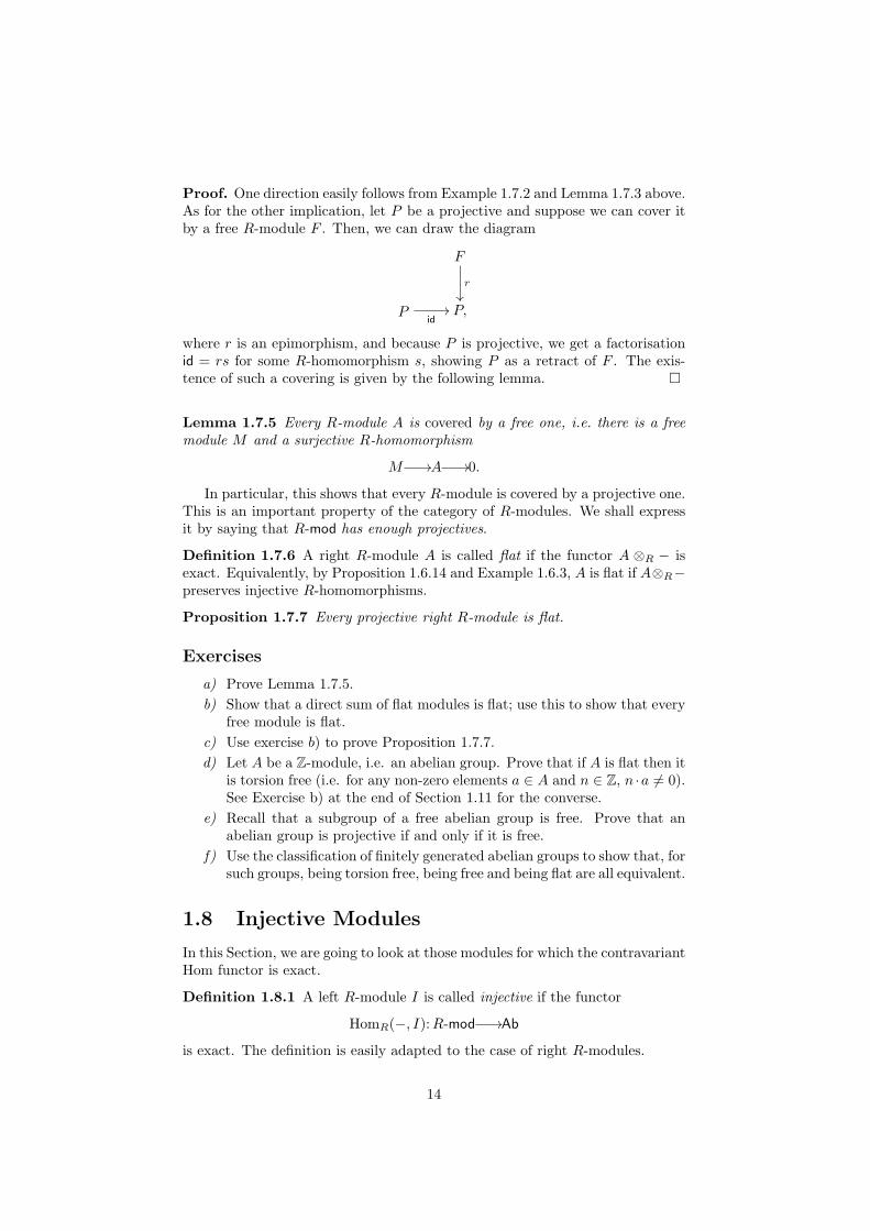
Proof. One direction easily follows from Example 1.7.2 and Lemma 1.7.3 above.As for the other implication, let P be a projective and suppose we can cover itby a free R-module F . Then, we can draw the diagram

F

r

²²

Pid

// P,

where r is an epimorphism, and because P is projective, we get a factorisationid = rs for some R-homomorphism s, showing P as a retract of F . The exis-tence of such a covering is given by the following lemma. ¤

Lemma 1.7.5 Every R-module A is covered by a free one, i.e. there is a freemodule M and a surjective R-homomorphism

M //A //0.

In particular, this shows that every R-module is covered by a projective one.This is an important property of the category of R-modules. We shall expressit by saying that R-mod has enough projectives.

Definition 1.7.6 A right R-module A is called flat if the functor A ⊗R − isexact. Equivalently, by Proposition 1.6.14 and Example 1.6.3, A is flat if A⊗R−preserves injective R-homomorphisms.

Proposition 1.7.7 Every projective right R-module is flat.

Exercises

a) Prove Lemma 1.7.5.b) Show that a direct sum of flat modules is flat; use this to show that every

free module is flat.c) Use exercise b) to prove Proposition 1.7.7.d) Let A be a Z-module, i.e. an abelian group. Prove that if A is flat then it

is torsion free (i.e. for any non-zero elements a ∈ A and n ∈ Z, n ·a 6= 0).See Exercise b) at the end of Section 1.11 for the converse.

e) Recall that a subgroup of a free abelian group is free. Prove that anabelian group is projective if and only if it is free.

f) Use the classification of finitely generated abelian groups to show that, forsuch groups, being torsion free, being free and being flat are all equivalent.

1.8 Injective Modules

In this Section, we are going to look at those modules for which the contravariantHom functor is exact.

Definition 1.8.1 A left R-module I is called injective if the functor

HomR(−, I):R-mod //Ab

is exact. The definition is easily adapted to the case of right R-modules.

14

More concretely, I is injective if, for any two R-homomorphisms i:A //Band φ:A //I with i injective, there exists an extension ψ:B //I making thefollowing commute:

Aφ

//

²²

i

²²

I.

B

ψ

??

Notice that the notions of injective and projective module are dual; that is,we can write one from the other by “reversing the arrows”. More formally, anobject is injective in a category if and only if it is projective in its opposite(see Definition A.0.8). This enables us to translate a few results for projectivemodules to dual statements for injective ones. For instance, since the dual of aretract is again a retract, we have the following.

Proposition 1.8.2 Every retract of an injective module is injective.

Proposition 1.8.3 Let (Aj)j∈J be a family of R-modules and let A be theirdirect product. Then, A is injective if and only if each Ai is.

When R is the commutative ring Z, we can give a precise characterisationof injective modules.

Definition 1.8.4 An abelian group D is called divisible if, for any d ∈ D andany non-zero integer n, there is an element x ∈ D such that nx = d.

Example 1.8.5 The additive group Q of rational numbers is divisible. Also,any quotient of a divisible group is itself divisible.

Any element d in an abelian group D determines a (unique) group homo-morphism f :Z //D such that f(1) = d. Likewise, any n ∈ Z determines amorphism n ·−:Z //Z, and this will be injective if n 6= 0. The group D is thendivisible if there exists a g:Z //D making the following triangle commute (sothat, by setting x = g(1), we have d = f(1) = g(n · 1) = nx):

Z²²

n·−²²

f// D.

Zg

>>

This proves the following.

Proposition 1.8.6 Every injective Z-module is divisible.

The converse is also true.

Proposition 1.8.7 Every divisible abelian group is injective as a Z-module.

Proof. Let D be a divisible group an consider a diagram of abelian groups

A′φ

//

²²

i

²²

D

A

15

where i is injective. We wish to extend φ along i. Consider the set X of pairs(B,ψ) such that B is a subgroup of A containing A′ and ψ:B //D extendsφ. Define a partial order on X by saying that (B1, ψ1) ≤ (B2, ψ2) if B1 ⊂ B2

and ψ2 extends ψ1. Then, (X,≤) is clearly an inductive set, hence by Zorn’sLemma it has a maximal element (B0, ψ0).

Suppose B0 6= A, and let a ∈ A−B0. Then, the subgroup

B′ = b+ na : b ∈ B0, n ∈ Z

properly contains B0. If na /∈ B0 for all non-zero integers n, then ψ0 can beextended to a homomorphism ψ′:B′ //D by defining

ψ′(b+ na) = ψ0(b).

Otherwise, let m be the least positive integer such that ma ∈ B0, and letd = ψ0(ma). Then, define the extension ψ′:B′ //D of ψ0 as

ψ′(b+ na) = ψ0(b) + nx,

where x ∈ D is such that mx = d.In either case, the pair (B′, ψ′) violates the maximality of (B0, ψ0), therefore

B0 = A. This shows that D is injective. ¤

Example 1.8.8 By Example 1.8.5, it follows immediately that the rationalcircle Q/Z is divisible, hence injective.

We are now interested in showing that, every R-module can be embeddedinto an injective one. In order to prove this result, we shall first restrict ourattention to the case R = Z. Then, we shall be able to transpose the propertyto other categories of modules by means of an appropriate adjunction.

For the moment, let us define, for any abelian group A, a group Aˇas

Aˇ= HomZ(A,Q/Z).

Notice that there is a canonical homomorphism of abelian groups

α:A //(A ) (1.7)

defined by α(a)(φ) = φ(a) for any a in A and φ ∈ HomZ(A,Q/Z).

Lemma 1.8.9 The group homomorphism α of (1.7) is injective.

Proof. It is clearly enough to prove that for any a 6= 0 in A there is a morphismφ:A //Q/Z with φ(a) 6= 0. Using injectivity of Q/Z, it is enough to define φon the subgroup B of A generated by a. If na 6= 0 for all n ∈ Z, then B is afree Z-module with base a, and we may choose φ so that φ(a) is any non-zeroelement of Q/Z. Otherwise, let m be the least positive integer such that ma = 0and define φ(na) as the class of n/m in Q/Z. In both cases, φ satisfies the re-quired property. ¤

Lemma 1.8.10 If A is a flat Z-module, then Aˇ is divisible.

16

Proof. Equivalently, we show that Aˇ is an injective abelian group. To thispurpose, suppose

Bf

//

i

²²

Aˇ

B′,

are group homomorphisms, with i injective. Then, the diagram transposesthrough the isomorphism (1.2) to give

B ⊗Z Af ′

//

i⊗idA

²²

Q/Z

B′ ⊗Z A,

where i⊗ idA is injective because A is flat.Hence, by Example 1.8.8, there is an extension g′:B′ ⊗Z A //Q/Z, which

transposes back to give a group homomorphism

g:B //Aˇ

such that gi = f . ¤

Theorem 1.8.11 Every abelian group can be embedded into an injective one.

Proof. By Lemma 1.7.5, we can cover the Z-module Aˇwith a free one, i.e.there is an exact sequence

Fq

// Aˇ // 0 (1.8)

where F is free. By applying the contravariant functor HomZ(−,Q/Z) to (1.8),we obtain an exact sequence

0 // (A )q∗

// F .

Hence, q∗: (A ) //Fˇis injective and, by Lemma 1.8.9, so is the composite

Aα //(A )

q∗//F .

Moreover, Fˇis injective by Lemma 1.8.10, whence the result. ¤

Analogously to the case of projectives, this property of categories of modulesis very important, and we shall express it by saying that Z-mod has enoughinjectives.

Now, we can use Theorem 1.8.11 to prove that the category R-mod hasenough injectives for any ring R. This will use a standard proof technique, whichrelies on the following categorical lemma (see the Appendix for the relevantdefinitions).

17

Lemma 1.8.12 If F aG: C //D is a pair of adjoint functors and F preservesmonos, then G preserves injectives.

Theorem 1.8.13 Every left R-module can be embedded into an injective one.

Proof. Let φ:Z //R be the unique morphism of rings fixing u(1) = 1. Then,by Theorem 1.5.4, we have an adjunction

Z-modφ∗

⊥ 22 R-mod

φ∗rr

and by Theorem 1.8.11 we can, for any R-module A, consider the embedding

φ∗A //γ

// D

of the abelian group φ∗A into an injective D.Since right adjoint functors preserve monomorphisms, φ∗γ is again mono.

Moreover, the unit of the adjunction η:A //φ∗φ∗A = HomZ(R,A) computesas η(a)(r) = ra, therefore it is obviously injective. The transpose

γ = Aη

// φ∗φ∗Aφ∗γ // φ∗D

of γ along the adjunction is then itself mono, and φ∗D is injective by Lemma1.8.12, since φ∗ preserves monos; therefore, we have the desired embedding. ¤

Exercises

a) Prove Proposition 1.8.3.b) Prove Lemma 1.8.12.

1.9 Complexes

In Section 1.6 we have investigated the concept of an exact sequence. In par-ticular, these chains of morphisms satisfy the property that the composite ofany two consecutive maps is null. Complexes, and their homology, enable oneto study how far a sequence of modules is from being exact.

Definition 1.9.1 A chain complex C? of R-modules is a Z-indexed sequence ofR-modules and R-homomorphism

· · · Cn−1oo Cn

dnoo Cn+1dn+1

oo · · ·oo (1.9)

such that dn dn+1 = 0 for all n ∈ Z. The maps dn are called boundary maps,and we shall omit the index whenever possible. An element of Cn is called ann-chain.

18

A morphism of chain complexes f?:C? //C ′? is a family (fn:Cn //C ′n)n∈Zof R-homomorphisms, such that the following diagram commutes for all n ∈ Z:

Cndn //

fn

²²

Cn−1

fn−1

²²

C ′nd′n

// C ′n−1.

We shall often drop the subscripts, and express this condition by saying thatfd = df . Two morphisms of chain complexes f?:C? //C ′? and g?:C ′? //C ′′?can be composed degree by degree, to give the morphism g? f? = (gn fn)n∈Z.Moreover, for any chain complex C? there is an obvious identity morphismidC?

= (idCn)n∈Z. Thus, we have a category of chain complexes, which we

denote by Ch(R).

Definition 1.9.2 The category Ch+(R) of positive chain complexes is definedto be the (full) subcategory of Ch(R) whose objects are those chain complexesC? with Cn = 0 for n < 0.

Similarly, we define the category Chb(R) of bounded chain complexes, whoseobjects are those chain complexes C? such that Cn = 0 for all but finitely manyvalues of n.

As for many categorical notions, that of a chain complex has a dual.

Definition 1.9.3 A cochain complex C? of R-modules is a sequence of modulesand maps

· · · // Cn−1 dn−1// Cn

dn// Cn+1 // · · · (1.10)

with the property d d = 0. An element of Cn is called an n-cochain.Morphisms of cochain complexes are defined in the obvious way, by the

condition fd = df , and they compose, to form a category of cochain complexes,denoted by CCh(R). This admits a subcategory of positive cochain complexesCCh+(R) and a subcategory of bounded cochain complexes CChb(R), defined inthe obvious way.

Notice that, for categories of (co)chain complexes, it makes sense to speakof short exact sequences. In particular, we shall say that

0 //A?f

//B?g

//C? //0

is an exact sequence of (co)chain complexes if the short sequence of R-modules

0 //Anfn //Bn

gn //Cn //0

is exact for each n ∈ Z.

Example 1.9.4 The standard p-simplex ∆p ⊂ Rp+1 is defined as the set

∆p =

(x0, . . . , xp) :

p∑

i=0

xi = 1, xi ≥ 0 for all i = 0, . . . , p

.

19

The face operators ∂i:∆p−1//∆p (i = 0, . . . , p) are defined by

∂i(x0, . . . , xp−1)) = (x0, . . . , xi−1, 0, xi, . . . , xp−1).

A singular p-simplex in a topological space X is a continuous functions:∆p

//X. For any p ≥ 0, the set of all singular p-simplices in X is denotedby ∆p(X). The space Cp(X) of singular p-chains on X is the free Z-modulegenerated by ∆p(X).

Precomposition with ∂i takes any p-simplex s:∆p//X to a (p− 1)-simplex

s ∂i. Since ∆p(X) is a basis of Cp(X), these maps extend uniquely to linearmaps

di:Cp(X) //Cp−1(X).

The boundary operator d:Cp(X) //Cp−1(X) (p > 0) is by definition the linearmap

d =p∑

i=0

(−1)idi

taking a singular p-chain α to dα =∑pi=0(−1)iα ∂i.

The sequence of chain groups

· · · Cp−1(X)doo Cp(X)doo · · ·doo

is a positive chain complex. We call C?(X) the singular complex of X.Moreover, any continuous map f :X //Y determines by postcomposition

a morphism of chain complexes f?:C?(X) //C?(Y ). We shall look at this inmore detail in Chapter 3.

Example 1.9.5 If M is an n-dimensional smooth manifold, define:

O(M) = f :M //R : f is a C∞-function.We denote by Ωp(M) (p ≥ 0) the O(M)-module of differential p-forms on M ,which is generated by elements dxi1 ∧ · · · ∧ dxip , subject to the condition

dxi1 ∧ · · · ∧ dxip = (−1)ldxτi1 ∧ · · · ∧ dxτipfor any permutation τ of i1, . . . , ip of degree l. Therefore, any element ω inΩp(M) is uniquely written as

ω =∑

i1<···<ipfi1···ipdxi1 ∧ · · · ∧ dxip (1.11)

with fi1...ip a C∞-function.The exterior derivative d: Ωp(M) //Ωp+1(M) is inductively defined as fol-

lows. If f ∈ Ω0(M) = O(M), then

df =n∑

j=1

∂f

∂xjdxj .

If p > 0 and ω ∈ Ωp(M) is a p-form as in (1.11), then we define

dω =∑

i1<···<ipdfi1···ip ∧ dxi1 ∧ · · · ∧ dxip .

20

The exterior derivative gives a bounded cochain complex Ω?(M), called the deRham complex of M :

0 // Ω0(M) d // Ω1(M) d // · · · d // Ωn(M) // 0.

Note that the condition dn dn+1 = 0 for a chain complex is equivalentto im(dn+1) ⊂ ker(dn). This is half of the condition needed for exactness. Inparticular, it enables us to form the quotient groups ker(dn)/ im(dn+1), whichwill somehow measure “how far a complex is from being exact”.

Definition 1.9.6 The n-th homology group of the chain complex C? is definedas:

Hn(C?) = ker(dn)/ im(dn+1).

The elements of Hn(C?) are called homology classes. They are represented byn-chains in ker(dn) (these are called n-cycles), up to a summand in im(dn+1)(which are called n-boundaries). The homology class represented by a cycle cis denoted by [c] = c+ im(dn+1) ∈ Hn(C?). The sum of [x] and [y] is given bythe class [x + y], and the null class 0 is represented by x if and only if x = dyfor some y ∈ Cn+1.

Analogously, for a cochain complex C?, we define its cohomology group indegree n as the quotient

Hn(C?) = ker(dn)/ im(dn−1).

A cochain x in Cn is a cocycle if dnx = 0 and a coboundary if x = dy for somey ∈ Cn−1. The equivalence class of a cocycle x is called the cohomology class ofx, and it is denoted by [x].

Example 1.9.7

a) The homology groups Hn(C?(X)) of the singular complex of Example 1.9.4above are called the singular homology groups of the space X, and are usuallydenoted by Hi(X);b) The p-th cohomology group Hp(Ω?(M)) of the complex of Example 1.9.5 isdenoted by Hp

dR(M) and it is called the p-th de Rham cohomology group of themanifold M .

A morphism of (co)chain complexes f?:C? //C ′? clearly maps (co)cycles to(co)cycles and (co)boundaries to (co)boundaries. Therefore, it induces in eachdimension n a homomorphism

Hn(f):Hn(C?) //Hn(C ′?)

defined as Hn(f)([c]) = [fn(c)]. We shall often simply write f , or f∗, for Hn(f).As usual, we have functoriality: if f?:C? //C ′? and g?:C ′? //C ′′? are mor-phisms of (co)chain complexes, then (g f)∗ = g∗ f∗ and id∗ = idHn(C?) foreach n. Thus each Hn is a covariant functor from Ch(R) (respectively, CCh(R))to R-mod.

21

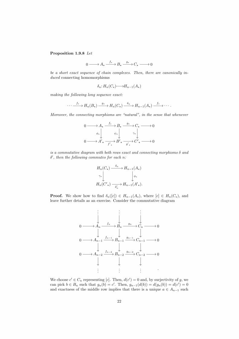
Proposition 1.9.8 Let

0 // A?f? // B?

g? // C? // 0

be a short exact sequence of chain complexes. Then, there are canonically in-duced connecting homomorphisms

δn:Hn(C?) //Hn−1(A?)

making the following long sequence exact:

· · · f∗ // Hn(B?)g∗ // Hn(C?)

δn // Hn−1(A?)f∗ // · · · .

Moreover, the connecting morphisms are “natural”, in the sense that whenever

0 // A?f? //

φ?

²²

B?g? //

ψ?

²²

C? //

γ?

²²

0

0 // A′?f ′?

// B′?g′?

// C ′? // 0

is a commutative diagram with both rows exact and connecting morphisms δ andδ′, then the following commutes for each n:

Hn(C?)δn //

γ∗²²

Hn−1(A?)

φ∗²²

Hn(C ′?)δ′n

// Hn−1(A′?).

Proof. We show how to find δn([c]) ∈ Hn−1(A?), where [c] ∈ Hn(C?), andleave further details as an exercise. Consider the commutative diagram

...

²²

...

²²

...

²²

0 // Anfn //

²²

Bngn //

²²

Cn //

²²

0

0 // An−1fn−1

//

²²

Bn−1gn−1

//

²²

Cn−1//

²²

0

0 // An−2fn−2

//

²²

Bn−2gn−2

//

²²

Cn−2//

²²

0

......

....

We choose c′ ∈ Cn representing [c]. Then, d(c′) = 0 and, by surjectivity of g, wecan pick b ∈ Bn such that gn(b) = c′. Then, gn−1(d(b)) = d(gn(b)) = d(c′) = 0and exactness of the middle row implies that there is a unique a ∈ An−1 such

22

that fn−1(a) = d(b). Therefore, fn−2(d(a)) = d(fn−1(a)) = d(d(b)) = 0, and byinjectivity of fn−2 we get d(a) = 0, so we define δn([c]) = [a] ∈ Hn−1(A?). Morediagram chasing proves that [a] is independent of the choices of c′ ∈ [c] andb ∈ Bn such that gn(b) = c′. Naturality of δ is proved by analogous techniques.

¤

Exercise

a) Fill in the details of the proof of Proposition 1.9.8. Then, formulate theanalogous result for cochain complexes.

1.10 Homotopy of chain complexes

We shall now focus on chain complexes, although this is inessential, and wecould easily restate every result for cochain complexes.

Definition 1.10.1 Let f, g:C? //C ′? be two morphisms of chain complexes.Then, a chain homotopy between f and g is a sequence of homomorphismshn:Cn //C ′n+1 (n ∈ Z) such that, for all n,

fn − gn = d′n+1 hn + hn−1 dn. (1.12)

We shall often omit the subscripts, and write (1.12) as f − g = hd+ dh. Picto-rially, the situation is represented in the diagram below:

· · · Cn−1oo

hn−1

%%

fn−1

²²

gn−1

²²

Cndnoo

hn

%%

fn

²²

gn

²²

Cn+1dn+1

oo

fn+1

²²

gn+1

²²

· · ·oo

· · · C ′n−1oo Cn

d′n

oo Cn+1d′n+1

oo · · ·oo

Example 1.10.2 Homotopies between maps of topological spaces induce chainhomotopies. We shall investigate this further in Chapter 3.

Remark 1.10.3 We define an equivalence relation between maps of chain com-plexes by saying that f is equivalent to g if there is a homotopy from f to g.(This is indeed an equivalence relation, by Exercise a) below.) We denote thisrelation by writing f ∼ g, and say in this case that f and g are homotopic.Notice that it is respected by composition:

Proposition 1.10.4 Consider the following diagram of chain complexes:

C?f

//

g// C ′?

h //

i// C ′′?.

If f ∼ g and h ∼ i, then h f ∼ i g.

The proof of this result is left as an exercise.

23

Remark 1.10.5 This shows that the relation of being homotopic is preservedby composition. In particular, this allows one to define the quotient categories

Ho(R), Ho+(R) and Hob(R)

of Ch(R), Ch+(R) and Chb(R) respectively. These will have the same objects astheir corresponding categories of complexes, but as maps homotopy equivalenceclasses of maps of chain complexes.

Homology can not distinguish homotopic maps:

Proposition 1.10.6 If f ∼ g:C? //C ′? are homotopic maps of chain com-plexes, then they induce the same maps between the homology groups:

f∗ = g∗:Hn(C?) //Hn(C ′?).

Proof. Suppose h is a homotopy between f and g. Then, we want to showthat the difference f∗ − g∗ is the null map between the homology groups. Tothis purpose, let [c] ∈ Hn(C?) for some c ∈ ker dn. Then,

(fn − gn)(c) = (d′n+1hn + hn−1dn)(c) = d′n+1(hn(c));

that is, (fn − gn)(c) is an n-boundary in C ′n. Hence,

(f∗ − g∗)([c]) = [(fn − gn)(c)] = 0

for all [c] ∈ Hn(C?). ¤

Definition 1.10.7 A morphism f?:C? //C ′? of chain complexes is a homotopyequivalence if there exists another morphism g?:C ′? //C? such that f g ∼ idC′and g f ∼ idC .

From Proposition 1.10.6 we obtain immediately:

Corollary 1.10.8 A homotopy equivalence f?:C? //C ′? induces isomorphismsf∗:Hn(C?) //Hn(C ′?) between the homology groups in each degree n.

Definition 1.10.9 A morphism f?:C? //C ′? of chain complexes is said to be aquasi-isomorphism if the corresponding homology maps f∗:Hn(C?) //Hn(C ′?)are isomorphisms for all n ∈ Z.

Remark 1.10.10 It is obvious by the definitions and Proposition 1.10.6 thatevery homotopy equivalence is also a quasi-isomorphism. The converse is nottrue (see Exercise d) below).

Definition 1.10.11 A resolution A P?εoo of a module A is an exact sequence

of modules0 Aoo P0

εoo P1oo · · ·oo

The resolution is called projective if so are all the modules Pn, for n ∈ Z. Dually,

an injective resolution Aη

//I? of A is an exact sequence:

0 // Aη

// I0 // I1 // · · ·where each In is injective.

24

Lemma 1.10.12 Given a map f :A //A′ of modules, a projective resolution

A P?εoo of A and any resolution A′ B?

ε′oo of A′, there is a morphismf?:P? //B? of exact sequences lifting f , in the sense that ε′f0 = fε:

0 Aoo

f

²²

P0εoo

f0

²²

P1d1oo

f1

²²

P2d2oo

f2

²²

· · ·d3oo

0 A′oo B0ε′

oo B1d′1

oo B2d′2

oo · · · .d′3

oo

(1.13)

Furthermore, the morphism f? is unique up to homotopy.

Proof. Since P0 is projective and ε′ is surjective, we can find f0 to make

A

f²²

P0εoo

f0²²

A′ B0ε′

oo

commute. It is easy to check that f0 restricts to a map F0: ker(ε) // ker(ε′),and by surjectivity of B1

// ker(ε′) we can find f1 making

ker(ε)

F0²²

P1oo

f1²²

ker(ε′) B1oo

commute. By iterating this construction, we define fn for all n ∈ Z.If g?:P? //B? is another morphism of exact sequences making (1.13) com-

mute, then f?− g? covers the morphism 0 = f − f :A //A′. Therefore, unique-ness follows if we show that f? is homotopic to zero whenever f = 0. To give ahomotopy, we need maps hn:Pn //Bn+1 (n ≥ 0) so that

fn = d′n+1hn + hn−1dn.

We are going to define them inductively. For n = 0, this reads f0 = d′1h0,and since P0 is projective, the existence of h0 follows from the exactness of thebottom row and the commutativity of the following:

A

0²²

P0oo

f0²²

h0

$$

A′ B0oo B1.

d′1

oo

For the inductive step, suppose the maps hi are defined for i < n and considerthe diagram

Pn−1

fn−1²²

hn−1

MMMM

&&MMMM

Pndnoo

fn

²²

hn

&&

Bn−1 Bnd′n

oo Bn+1.d′n+1

oo

25

The bottom row is exact and Pn is projective, so we can find a factorisationfn − hn−1dn = d′n+1hn provided we verify that d′n(fn − hn−1dn) = 0. But, bythe inductive hypothesis, we know that d′nhn−1 = fn−1 − hn−2dn−1, therefore

d′n(fn − hn−1dn) = d′nfn − fn−1dn + hn−2dn−1dn = d′nfn − fn−1dn = 0.

¤

Proposition 1.10.13 Every module A has a projective resolution, which isunique up to homotopy.

Proof. We know by the comment after Lemma 1.7.5 that A can be covered bya projective, i.e. there is a projective module P0 and an exact sequence

0 Aoo P0ε=ε0oo ker(ε0)

ι1oo 0oo

Similarly, the module ker(ε0) gives rise to an exact sequence

0 ker(ε0)oo P1ε1oo ker(ε1)

ι2oo 0oo

and so on for ker(εn), for each n ∈ Z. By Proposition 1.6.4, we can splice allthese short exact sequences into one long exact sequence:

0 Aoo P0εoo P1

d1oo

ε1ss

P2d2oo

ε2ss

· · ·oo

ker(ε)ι1

bb

ker(ε1)ι2

bb

This gives the desired resolution, and uniqueness follows by Lemma 1.10.12. ¤

The dual of the last two results, for injective resolutions, is also valid. Wewill come back to this duality in a more general context in Chapter 4. Theproofs of the following statements are analogous to the previous ones, and areleft as an exercise.

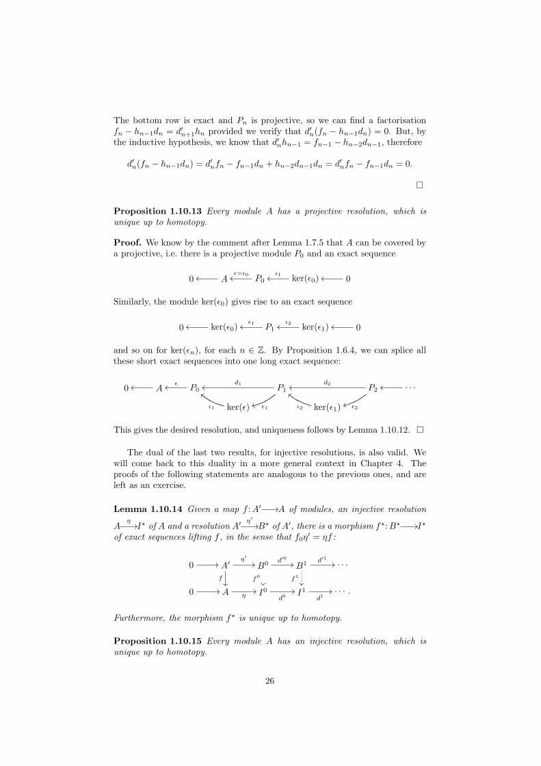
Lemma 1.10.14 Given a map f :A′ //A of modules, an injective resolution

Aη

//I? of A and a resolution A′η′

//B? of A′, there is a morphism f?:B? //I?

of exact sequences lifting f , in the sense that f0η′ = ηf :

0 // A′η′

//

f²²

B0 d′0 //

f0

²²

B1 d′1 //

f1

²²

· · ·

0 // A η// I0

d0// I1

d1// · · · .

Furthermore, the morphism f? is unique up to homotopy.

Proposition 1.10.15 Every module A has an injective resolution, which isunique up to homotopy.

26

Exercises

a) Show the relation∼ of Remark 1.10.3 to be in fact an equivalence relation.b) Prove Proposition 1.10.4.c) Prove Corollary 1.10.8.d) Show by an example that a quasi-isomorphism between chain complexes

need not be a homotopy equivalence.

1.11 Double Complexes

Just as we have exact sequences of chain complexes, we can formalise the conceptof a chain complex of chain complexes. This is usually achieved by using twoindexes. For this reason, we call these structures double complexes.

Definition 1.11.1 A double complex of R-modules C?? is a family Cp,q ofmodules together with maps:

dh:Cp,q //Cp,q+1 and dv:Cp,q //Cp+1,q

such that dhdh = dvdv = dvdh + dhdv = 0. Pictorially, C?? is a diagram

...

²²

...

²²

...

²²

· · · // Cp−1,q−1dh //

dv²²

Cp−1,qdh //

dv²²

Cp−1,q+1 //

dv²²

· · ·

· · · // Cp,q−1dh //

dv²²

Cp,qdh //

dv²²

Cp,q+1 //

dv²²

· · ·

· · · // Cp+1,q−1dh //

²²

Cp+1,qdh //

²²

Cp+1,q+1 //

²²

· · ·

......

...

in which each row C?,q and each column Cp,? is a cochain complex and, further-more, each square anti-commutes. Morphisms of double complexes are definedin an obvious way.

A double complex is called bounded, if there are only finitely many non-zeromodules on each diagonal p + q = n. A special case of this situation is whenboth the rows and the columns are positive complexes, that is to say, Cp,q = 0unless p, q ≥ 0. We call C?? positive in this case.

Definition 1.11.2 Given a bounded double complex C??, define the total com-plex Tot(C)? by:

Tot(C)n =⊕p+q=n

Cp,q.

The formula d = dh + dv defines a total differential

D: Tot(C)n // Tot(C)n+1 (1.14)

27

making Tot(C)? into a cochain complex. The action ofD on an element x ∈ Cp,qmaps it to (dhx, dvx) ∈ Cp,q+1 ⊕ Cp+1,q. Naively, we could think of the totalcomplex as “summing up C?? along the diagonals p+ q = n”.

Remark 1.11.3 In the definition of double complexes we could have just aswell required commutativity of each square, instead of anti-commutativity. Inother words, the equation dhdv+dvdh = 0 could be replaced by dvdh−dhdv = 0.We can always move from one convention to the other by replacing signs in theappropriate way. For instance, we can replace the maps dh:Ap,q //Ap+1,q bythe maps

δh = (−1)pdh:Cp,q //Cp,q+1,

or analogously for the vertical maps dv. The definition of the differential mapsin the associated total complex will then have to be adjusted according to theconvention.

Remark 1.11.4 Notice that a positive double complex C?? can always be aug-mented by adding in front of each row and each column the kernel of the appro-priate map. If we denote them by

H0h(C

?,0) = ker(d?,0h ) and H0v (C

0,?) = ker(d0,?h ),

then the complex takes the shape

H0v (C

0,0)dh //

²²

H0v (C

0,1) //

²²

· · ·

H0h(C

0,0) //

dv

²²

C0,0dh //

dv

²²

C0,1 //

dv

²²

· · ·

H0h(C

1,0) //

²²

C1,0dh //

²²

C1,1 //

²²

· · ·

......

....

(1.15)

The top row and the leftmost column of this augmented double complex arethemselves cochain complexes, which we denote by H0

v (C??) and H0

h(C??), re-

spectively. The cohomology of these complexes are denoted by Hnv (H0

h(C??))

and Hnh (H0

v (C??)).

The cohomology of these two cochain complexes is helpful in calculating thecohomology of the total complex associated to C??.

Lemma 1.11.5 (Double Complex Lemma) If C?? is a positive double com-plex with exact columns and exact rows, then there are canonical isomorphisms,for all n ≥ 0:

Hn(Tot(C)?) ' Hnv (H0

h(C??)) ' Hn

h (H0v (C

??)).

28

Proof. We picture the double complex Cp,q as in (1.15), with the p’s runningvertically and the q’s horizontally. By symmetry, it is sufficient to show that

Hn(Tot(C)?) ' Hnv (H0

h(C??)).

There is a natural group homomorphism

φ:Hnv (H0

h(C??)) //Hn(Tot(C)?)

taking the class [an,0] to [(an,0, 0, . . . , 0)]. To prove that φ is an isomorphism,we are going to produce its inverse ψ. To this purpose, it is enough to showthat any equivalence class x = [(a0, . . . , an)] ∈ Hn(Tot(C)?) can be uniquelywritten as [(b0, 0, . . . , 0)] for an opportune b0, and then define ψ(x) = [b0]. Moregenerally, we prove that if x = [(a0, · · · , ak, 0, · · · , 0)] for some 1 ≤ k ≤ n, thenx = [(b0, · · · , bk−1, 0, · · · , 0)], for opportune bi’s. The thesis will then follow byiterating the argument n-many times.

So, suppose x = [(a0, · · · , ak, 0, · · · , 0)]; then, post-composing D with theprojection π: Tot(C)n+1 //Cn−k,k+1, we get

dh(ak) = dh(ak) + dv(0) = πD(x) = 0,

and by exactness of the (n − k)-th row, there exists e ∈ Cn−k,k−1 such thatdh(e) = ak. Now we have

[(a0, . . . , ak, 0, . . . , 0)]− [(a0, . . . , ak−1−dv(e), 0, . . . , 0)]= [(0, . . . , 0, dv(e), ak, 0, . . . , 0)]= [(0, . . . , 0, dv(e), dh(e), 0, . . . , 0)]= D[(0, . . . , 0, e, 0, . . . , 0)];

hence, x is represented by the class [(a0, . . . , ak−1−dv(e), 0, . . . , 0)].

We leave it to the reader to check that these maps φ and ψ are well-definedand inverse to each other.

Note that we only use the fact that the rows are exact. Similarly, in orderto prove Hn(Tot(C)?) ' Hn

h (H0v (C

??)), it is suffices to have the exactness ofthe columns. ¤

To close this section, we give an application of double complexes to the studyof R-modules.

Let A, B be R-modules. Let A P?εoo be a projective resolution of A and

Bη

//I? an injective resolution of B. We can then form the double complexHomR(P?, I?). The morphisms ε and η induce maps from HomR(P?, I?) to

29

HomR(A, I?) and HomR(P?, B):

HomR(A, I0) //

ε∗

²²

HomR(A, I1) //

ε∗

²²

· · ·

HomR(P0, B)η∗ //

²²

HomR(P0, I0) //

²²

HomR(P0, I1) //

²²

· · ·

HomR(P1, B)η∗ //

²²

HomR(P1, I0) //

²²

HomR(P1, I1) //

²²

· · ·

......

....

By projectivity of the Pn’s and injectivity of the In’s, we have that all the rowsand columns of the augmented double complex above are exact. Therefore, bythe double complex lemma, we have that

Hn(HomR(A, I?)) ' Hn(HomR(P?, B)).

Definition 1.11.6 The cohomology groups we have just constructed are calledthe Ext groups, and are denoted by Extn(A,B). More precisely, for each A, Bin R-mod we define:

Extn(A,B) = Hn(HomR(A, I?)) ' Hn(HomR(P?, B)).

Analogously, given projective resolutions A P?εoo and B Q?

δoo of twoR-modules A and B, we define the Tor groups Torn(A,B) as the homologygroups

Torn(A,B) = Hn(A⊗R Q?) ' Hn(P? ⊗R B).

Proposition 1.11.7 Let B be an R-module.

(i) For every R-module A we have Tor0(A,B) ' A⊗R B.

(ii) Given a short exact sequence 0→ A′ → A→ A′′ → 0 of R-modules, thereexists a natural long exact ‘Tor-sequence’

· · · → Tor1(A′′, B)→ A′ ⊗R B → A⊗R B → A′′ ⊗R B → 0.

Proof. Let B δ←− Q? be a projective resolution of B. Then, for every R-moduleA, the sequence

A⊗R Q1id⊗d1−−−→ A⊗R Q0

id⊗δ−−−→ A⊗R B → 0

is exact since A⊗− is right-exact. Hence coker id⊗ d1 ' A⊗R B. This provesitem (i) because Tor0(A,B) = coker id⊗ d1.

To prove item (ii) suppose we are given a short exact sequence 0 → A′ →A → A′′ → 0 of R-modules. Let B δ←− Q? be a projective resolution of B and

30

consider the following short exact sequence of chain complexes.

...

²²

...

²²

...

²²

0 // A′ ⊗Q1//

²²

A⊗Q1//

²²

A′′ ⊗Q1//

²²

0

0 // A′ ⊗Q0//

²²

A⊗Q0//

²²

A′′ ⊗Q0//

²²

0

0 0 0

Applying Proposition 1.9.8 on this short exact sequence then gives the desiredTor-sequence. ¤

Exercise

a) Show, using the double complex lemma, that the Tor groups are welldefined.

b) Working over the ring R = Z, prove that

Tor1(A,Z/n) = a ∈ A|n · a = 0.

Use the classification of finitely generated abelian groups to conclude thatA is torsion free if and only if Tor1(A,B) = 0 for every finitely generatedabelian group B.

1.12 The Kunneth formula

Let C and C ′ be chain complexes of right and left R-modules respectively. Thetotal complex of the double complex Cp,q = Cp ⊗R C ′q with boundary maps

d⊗ id:Cp,q //Cp−1,q and (−1)pid⊗ d:Cp,q //Cp,q−1

is called the tensor product of C and C ′ and is denoted by C⊗RC ′. Rememberits boundary formula is given by

D(c⊗ c′) = dc⊗ c′ + (−1)pc⊗ dc′ for c ∈ Cp and c′ ∈ C ′q. (1.16)

Remark 1.12.1 (i) Let A be a right R-module, B an (R,S)-bimodule andC a left S-module. There is an isomorphism

(A⊗R B)⊗S C → A⊗R (B ⊗S C)

determined by(a⊗ b)⊗ c 7→ a⊗ (b⊗ c).

31

(ii) The above generalizes as follows. Let C ′ and C ′′ be chain complexes ofright R-modules and left S-modules respectively, and let C be a chaincomplex of (R,S)-bimodules. Then there is an isomorphism of chain com-plexes

(C ′ ⊗R C)⊗S C ′′ ' C ′ ⊗R (C ⊗S C ′′).(iii) Let A and B be R-bimodules. There is an isomorphism

A⊗B → B ⊗Adetermined by a⊗ b 7→ b⊗ a. Given two chain complexes of R-bimodulesC and C ′, this generalizes as follows: there is an isomorphism C ⊗ C ′ 'C ′ ⊗ C, determined by

c⊗ c′ 7→ (−1)pqc′ ⊗ c, where c ∈ Cp and c′ ∈ C ′q.In the remainder of this section we will, when no confusion can arise, suppress

reference to the ring R in the notations for tensor products of R-modules andtensor products of chain complexes.

Let C and C ′ be chain complexes of right and left R-modules respectively.From the boundary formula (1.16), it follows that the tensor product c ⊗ c′ oftwo cycles is a cycle in C ⊗ C ′ and that the tensor product of a cycle and aboundary is a boundary. We thus have a well-defined homomorphism

⊕p+q=n

Hp(C)⊗Hq(C ′)→ Hn(C ⊗ C ′) : [c]⊗ [c′] 7→ [c⊗ c′],

which is called the homology product.

Theorem 1.12.2 (The Kunneth formula) Let R be a principal ideal do-main and let C and C ′ be chain complexes of right and left R-modules respec-tively. If the R-modules Ci are all free then, for each n, there is a natural shortexact ‘Kunneth sequence’

0→⊕p+q=n

Hp(C)⊗Hq(C ′)→ Hn(C⊗C ′)→⊕

p+q=n−1

Tor1(Hp(C),Hq(C ′))→ 0.

Definition 1.12.3 Generalizing the direct sum of modules we define the directsum

⊕i∈I Ci of a family of chain complexes of left (resp. right) R-modules

(Ci)i∈I by(⊕

i∈ICi)n =

⊕

i∈I(Ci)n and d(ci) = (dci).

Clearly⊕

i∈I Ci is a chain complex of left (resp. right) R-modules and it caneasily be shown there exists a canonical isomorphism

Hn(⊕

i∈ICi) '

⊕

i∈IHn(Ci)

for each n. Moreover, if all of the Ci are chain complexes of right R-modulesand C ′ is a chain complex of left R-modules then, using Proposition 1.3.5, onecan prove there is a canonical isomorphism of chain complexes

(⊕

i∈ICi)⊗ C ′ '

⊕

i∈I(Ci ⊗ C ′).

32

Proof of Theorem 1.12.2. We shall use the fact that every submodule of a freeR-module is free if R is a principal ideal domain, see [3, Theorem III.7.1] forexample.

First assume C has trivial boundary morphisms. Then Hp(C) = Cp is freefor all p, hence the Tor1-term vanishes from the Kunneth sequence and we haveto show that the homology product is an isomorphism. Since the boundarymaps of C are trivial the boundary formula of C ⊗ C ′ becomes

D(c⊗ c′) = (−1)pc⊗ dc′ for c ∈ Cp and c′ ∈ C ′q,and one can easily show there is a canonical isomorphism of chain complexes

C ⊗ C ′ '⊕

p∈ZCp ⊗ C ′[p],

where Cp denotes the constant chain complex Cp with trivial boundary maps,and C ′[p] is given by C ′[p]n = C ′n−p, with boundary maps (−1)pd. Since Cp isfree it can be written as a disjoint sum of a family of R-modules Ri indexed bya set I, all of which are isomorphic to R. Hence

Hn(Cp ⊗ C ′[p]) '⊕

i

Hn−p(C ′) ' Cp ⊗Hn−p(C ′) = Hp(C)⊗Hn−p(C ′),

where we have used that Ri ⊗ C ′q ' C ′q and Hn(C ′[p]) = Hn−p(C ′). Summingover p thus gives an isomorphism

Hn(C ⊗ C ′) '⊕p+q=n

(Hp(C)⊗Hq(C ′)),

which one checks to be given by the homology product.In the general case, denote the kernels and the images of the boundary

homomorphisms of C by Zp ⊂ Cp and Bp ⊂ Cp respectively. They form chaincomplexes Z and B with trivial boundary maps and we have a short exactsequence 0 → Zp → Cp

d−→ Bp−1 → 0 in each degree p. Because Bp−1 isfree, we have Tor1(Bp−1, C

′q) = 0 in the associated long exact Tor-sequence (cf.

Proposition 1.11.7) and hence

0→ Zp ⊗ C ′q → Cp ⊗ C ′q → Bp−1 ⊗ C ′q → 0

is exact for each pair p and q. Summing over p+ q = n, these assemble to giveshort exact sequences

0→ (Z ⊗ C ′)n → (C ⊗ C ′)n → (B ⊗ C ′)n−1 → 0.

Since Z and B are chain complexes with trivial boundary maps we have by thespecial case above

Z ⊗ C ′ '⊕

p∈ZZp ⊗ C ′[p] and B ⊗ C ′ '

⊕

p∈ZBp ⊗ C ′[p].

For each degree n, these isomorphisms convert the exact sequence above intoan exact sequence that commutes with the respective boundary maps, so theyform an exact sequence of chain complexes

0→⊕

p∈ZZp ⊗ C ′[p]→ C ⊗ C ′ →

⊕

p∈ZBp−1 ⊗ C ′[p]→ 0.

33

Hence we have a long exact sequence in homology (cf. Proposition 1.9.8)

· · · →⊕p+q=n

Bp ⊗Hq(C ′)δn−→

⊕p+q=n

Zp ⊗Hq(C ′)→ Hn(C ⊗ C ′)

→⊕

p+q=n−1

Bp ⊗Hq(C ′)δn−1−−−→

⊕p+q=n−1

Zp ⊗Hq(C ′)→ · · · .

Notice that the connecting morphism δn is just the homomorphism given bythe homomorphisms Bp ⊗ Hq(C ′) → Zp ⊗ Hq(C ′) coming from the inclusionBp ⊂ Zp. Indeed, let b ⊗ [c′] belong to Bp ⊗ Hq(C ′). Pulling the cycle b ⊗ c′in Bp ⊗ C ′q back under d ⊗ id gives c ⊗ c′ in Cp+1 ⊗ C ′q, where d(c) = b, andD(c ⊗ c′) = b ⊗ c′ in Cp ⊗ C ′q since c′ is a cycle. Pulling the latter back underZp ⊗ C ′q → Cp ⊗ C ′q, which is induced by the inclusion Zp ⊂ Cp, gives b ⊗ c′,now seen as a tensor product in Zp ⊗ C ′q. The image of b⊗ [c′] in Bp ⊗Hq(C ′)under δn is thus b⊗ [c′] in Zp ⊗Hq(C ′).

Now the exactness in Hn(C ⊗C ′) of the long exact sequence above is equiv-alent to the exactness of the short exact sequence

0→ coker δn → Hn(C ⊗ C ′)→ ker δn−1 → 0,

which we will show to be the sequence of the theorem.For each p we have an exact sequence 0 → Bp → Zp → Hp(C) → 0, and

tensoring with Hq(C ′) gives the exact sequence

Bp ⊗Hq(C ′)→ Zp ⊗Hq(C ′)→ Hp(C)⊗Hq(C ′)→ 0.

Summing over p+ q = n these assemble to give the exact sequence⊕p+q=n

Bp ⊗Hq(C ′)δn−→

⊕p+q=n

Zp ⊗Hq(C ′)→⊕p+q=n

Hp(C)⊗Hq(C ′)→ 0,

hence coker δn =⊕

p+q=nHp(C)⊗Hq(C ′).To determine ker δn−1, again consider the exact sequence 0 → Bp → Zp →

Hp(C) → 0. Since Zp is free we have Tor1(Zp, Hq(C)) = 0 in the associatedlong exact Tor-sequence and hence the sequence below is exact.

0→ Tor1(Hp(C),Hq(C))→ Bp⊗Hq(C)→ Zp⊗Hq(C)→ Hp(C)⊗Hq(C)→ 0

Summing over p+ q = n− 1 we thus find

ker δn−1 =⊕

p+q=n−1

Tor1(Hp(C),Hq(C)),

which completes the proof of the theorem. The reader can check that every stepin the argument above is natural, so that the Kunneth sequence itself is natural.

¤

Since every module (vector space) over a field is free, we obtain

Corollary 1.12.4 Let K be a field and C and C ′ be chain complexes left andright K-modules respectively. Then the homology product

⊕p+q=n

Hp(C)⊗Hq(C ′)→ Hn(C ⊗ C ′)

is an isomorphism.

34

Definition 1.12.5 Let C be a chain complex of left R-modules. If M is anyright R-module, the homology of C with coefficients in M is given by

H∗(C;M) = H∗(C ⊗M).

Theorem 1.12.6 (Universal coefficient theorem for homology) Let C bea chain complex of free left modules over R and let M be a right R-module. Thenthere is a natural short exact sequence

0→ Hn(C)⊗M → Hn(C;M)→ Tor1(Hn−1(C),M)→ 0.

In particular, if R is a field then Hn(C;M) ' Hn(C)⊗M .

Proof. Apply Theorem 1.12.2 on C and C ′, where C ′0 = M and C ′n = 0 forn 6= 0. ¤

Proposition 1.12.7 The Kunneth sequence of Theorem 1.12.2 splits, yieldinga direct sum composition

Hn(C ⊗ C ′) '( ⊕p+q=n

Hp(C)⊗Hq(C ′)

)⊕

( ⊕p+q=n−1

Tor1(Hp(C),Hq(C ′))

).

Proof. We will show that the Kunneth sequence splits if both C and C ′ arefree. This suffices for our applications. It is not hard to generalize the argumentbelow to show splitting when C ′ is not free, see [2, Section V.2].

The exact sequence 0 → Zp → Cp → Bp−1 → 0 splits since Bp−1 is a free.Hence Cp ' Zp ⊕Bp−1 and we can thus extend the quotient map Zp → Hp(C)to a homomorphism Cp → Hp(C). Viewing H∗(C) as a chain complex H(C)with trivial boundary maps, these homomorphisms form a morphism of chaincomplexes C → H(C). Similarly we have a morphism of chain complexes C ′ →H(C ′) and tensoring these morphisms gives a morphism

C ⊗ C ′ → H(C)⊗H(C ′).

Now the chain complex H(C) ⊗ H(C ′) equals its own homology because itsboundary maps are trivial and the induced morphism on homology for the mor-phism of chain complexes above is the splitting map we sought. ¤

Remark 1.12.8 The splitting of the Kunneth sequence is not natural, as isdemonstrated by the following example.

If the splitting were natural then we would have, for any two morphisms ofchain complexes φ:C //D and ψ:C ′ //D′, that (φ ⊗ ψ)∗ = 0 if φ∗ ⊗ ψ∗ = 0and Tor1(φ∗, ψ∗) = 0. To give a counter-example to this implication, considerthe following situation. Take R = Z, C0 = Z = C1, Cn = 0 for n 6= 0, 1 andd1(1) = 2; D1 = Z, Dn = 0 for n 6= 1 and φ1 = id; C ′0 = Z/2Z, C ′n = 0 forn 6= 0, D′ = C ′ and ψ = id. Clearly φ∗ = 0, hence, assuming that the splittingis natural, we would have (φ⊗ψ)∗ = 0. However, (C⊗C ′)2 = 0 = (D⊗D′)2 andhence H1(C⊗C ′) = C1⊗C ′0 = Z⊗Z/2Z and H1(C⊗C ′) = D1⊗D′0 = Z⊗Z/2Z,so that (φ⊗ ψ)∗:H1(C ⊗ C ′) //H1(D ⊗D′) is an isomorphism.

35

1.13 Additional exercises

1. Let R be a ring with unit, A a right R-module and B a left R-module.Prove that R⊗R B ∼= B and A⊗R R ∼= A.

2. Compute Z/n⊗Z Q and Q⊗Z Q.

3. Show that Z/n⊗Z Z/m ∼= Z/d, where d = gcd(n,m).

4. Give an example of R-modules A and Bii∈I such that

A⊗R(∏

i∈IBi

)6∼=

∏

i∈I(A⊗R Bi) .

36

2. Cohomology of groups

In this Chapter, we use the machinery of cohomology introduced in Chapter 1in order to study properties of groups. To fix notation, our default group G(in multiplicative notation) will have elements g, h, and so on; its unit will bedenoted by 1.

2.1 Cohomology of a group

In order to introduce the concept of cohomology for an arbitrary group, wefirst need to generate a cochain complex. This will arise from the followingdefinitions.

Definition 2.1.1 Given a group G, we denote by Z[G] the free abelian groupon the underlying set of G. Multiplication of G clearly extends by distributivityto a multiplication on Z[G], making it into a ring. We call this the group ringon G.

There is an obvious ring epimorphism ε:Z[G] //Z, called the augmentationof G, determined by mapping every g ∈ G to 1. As we saw in Section 1.5, thisinduces a functor ε∗:Z-mod = Ab //Z[G]-mod.

Definition 2.1.2 A G-module A is an abelian group A (in additive notation),equipped with a left action by G for which the distributive law holds, i.e. a map

G×A //A (g, a) 7→ g · asuch that, for all a, b ∈ A and g, h ∈ G,

a) g · (a+ b) = g · a+ g · b;b) 1 · a = a;c) g · (h · a) = (gh) · a.

A morphism of G-modules f :A //B is a morphism of abelian groups whichrespects the action of G; namely, for all g ∈ G and a, a1, a2 ∈ A:

a) f(a1 + a2) = f(a1) + f(a2);b) f(g · a) = g · f(a).

G-modules and G-module morphisms form a category, denoted by G-mod.

Remark 2.1.3 Alternatively, we could define an action of a group G on anabelian group A as a group homomorphism

G // Aut(A),

37

where Aut(A) is the group of automorphisms of A, with composition as multi-plication and the identity on A as unit.

Example 2.1.4 Every abelian group A can be viewed as a trivial G-module,with the action g · a = a, for all g ∈ G and a ∈ A. This determines a trivialG-module functor from Ab to G-mod, which is the functor ε∗ of Definition 2.1.1.

Remark 2.1.5 The name G-module for such structures is not inappropriate.In fact, to give a G-module structure on an abelian group A is the same asgiving a Z[G]-module structure on it. More precisely, there is an isomorphismof categories G-mod ' Z[G]-mod.

Appealing to this isomorphism, we shall henceforth make no distinction be-tween a G-module and a Z[G]-module structure on an abelian group A.

Definition 2.1.6 For a G-module A, the subgroup

AG = a ∈ A | ga = a for all g ∈ G (2.1)

is called the subgroup of invariants of A. The quotient group

AG = A/〈ga− a | g ∈ G, a ∈ A〉

is the group of coinvariants of A. The assignments A 7→ AG and A 7→ AG definefunctors (−)G and (−)G from G-mod to Ab.

You should check that these functors have the property stated in the follow-ing proposition (cf. Exercise b) below):

Proposition 2.1.7 For a group G with augmentation ε:Z[G] //Z, there is achain of adjunctions

(−)G a ε∗ a (−)G.

By uniqueness of adjoints (see Exercise c) in the Appendix) and the resultsof Section 1.5, we obtain:

Corollary 2.1.8 For any group G, there are natural isomorphisms

AG ' Z⊗Z[G] A and AG ' HomZ[G](Z, A).

Now, we have all the tools needed to define the homology and cohomologyof groups. If A is a G-module, we can consider it as a Z[G]-module, by Remark2.1.5. Then, by Proposition 1.10.15, we can take an injective resolution of A

0 //A //I0 //I1 //I2 // · · · .

Applying now the functor (−)G:G-mod //Ab to this resolution, we obtain thecochain complex

(I0)G // (I1)G // (I2)G // · · · . (2.2)

Definition 2.1.9 We define the cohomology groups of G with coefficients in Aas the cohomology of the cochain complex (2.2), denoted by H∗(G;A).

38

Remark 2.1.10 Note that the notion is well-defined, because, by Proposition1.10.15, the injective resolution of A is unique up to homotopy, and we knowthat homotopic maps induce the same morphisms in homology.

Remark 2.1.11 We know from Corollary 2.1.8 that (−)G is naturally isomor-phic to HomZ[G](Z,−), so it follows that

H∗(G;A) ' H∗(HomZ[G](Z, I?)) = Ext∗Z[G](Z, A).

From the double complex lemma 1.11.5, we know that we can also computeExt∗Z[G](Z, A) by considering a projective resolution of Z in the category of(left) Z[G]-modules

0 Zoo P0oo P1

oo · · ·oo

and taking the cohomology of the cochain complex HomZ[G](P?, A):

HomZ[G](P0, A) // HomZ[G](P1, A) // HomZ[G](P2, A) // · · · .

It follows, that H∗(G;A) ' Ext∗Z[G](Z, A) ' H∗(HomZ[G](P?, A)), and theseisomorphisms are natural in A.

So far, we considered only cohomology of groups. Using the covariant functor(−)G:G-mod //Ab, we can define the homology groups of G with coefficientsin A in a dual way.

First, we consider a projective resolution of A as a Z[G]-module

0 Aoo Q0oo Q1

o o · · · ;oo

then, we apply the functor (−)G to this complex to get

(Q0)G (Q1)Goo · · ·oo (2.3)

Definition 2.1.12 The homology groups of G with coefficients in A, denotedH∗(G;A), are defined to be the homology of the chain complex (2.3); hence:H∗(G;A) = H∗((Q?)G).

Remark 2.1.13 As in the case of cohomology, this definition is correct, i.e.it does not depend on the choice of the projective resolution Q?. In fact, forany other resolution Q′?, the groups Hn((Q?)G) and Hn((Q′?)G) are naturallyisomorphic.

Moreover, for any projective resolution 0 Zoo P0oo P1

oo · · ·oo of Zas a Z[G]-module, we can compute these homology groups from the complex

P0 ⊗Z[G] A P1 ⊗Z[G] Aoo · · ·oo

Again by the double complex lemma, it follows that H∗(G;A) ' Tor∗(Z, A).

In these lectures, we shall focus on the cohomology of groups and leavehomology aside.

39

Exercises

a) Let U :Rng //Grp be the functor taking a ring R to the group U(R) ofinvertible elements in R (what is its action on maps?). Show that thereis an adjunction Z[−]aU .

b) Complete the definition of the functors (−)G and (−)G and show thatthere is a chain of adjunctions (−)G a ε∗ a (−)G, where ε∗ is the trivialG-module functor of Example 2.1.4. Using uniqueness of adjoints (seeexercise c) in the Appendix), explain how Corollary 2.1.8 follows.

2.2 Functoriality of cohomology

In this Section, we show that the cohomology groups H∗(G;A) are functorialin both A and G.

2.2.1 Functoriality in A

Suppose the group G is fixed. Then, for every n ∈ N, Hn(G;−):G-mod //Abis a functor which takes a G-module A to the n-th cohomology group of G withcoefficients in A, and a G-module morphism ϕ:A //B to the map

ϕ∗ = Hn(G;ϕ):Hn(G;A) //Hn(G;B) (2.4)

induced by HomZ[G](Pn, A) // HomZ[G](Pn, B).In detail, let 0 Zoo P?oo be a projective resolution of the trivial left

Z[G]-module Z. By applying HomZ[G](−, A) and HomZ[G](−, B) to this se-quence, and merging the two with the morphism ϕ∗ of Remark 1.2.3, we get amorphism of cochain complexes

HomZ[G](P0, A) //

ϕ∗²²

HomZ[G](P1, A) //

ϕ∗²²

· · ·

HomZ[G](P0, B) // HomZ[G](P1, B) // · · · .

The desired map ϕ∗ is now defined by functoriality of Hn for these chain com-plexes and this chain map.

Note that ϕ∗ does not depend on the projective resolution of Z, for if thereis an other projective resolution 0 Zoo Q?oo , then we have natural iso-morphisms

Hn(HomZ[G](Pn, A))ϕ∗P //

'²²

Hn(HomZ[G](Pn, B))

'²²

Hn(HomZ[G](Qn, A))ϕ∗Q

// Hn(HomZ[G](Qn, B)).

Remark 2.2.1 We could have computed the map ϕ∗ using injective resolutionsof A and B and lifting ϕ to a chain map. However, using a projective resolution

40

of Z reveals an important property of the cohomology of groups. Namely, ifthere is a short exact sequence of G-modules

0 // Aϕ

// Bψ

// C // 0,

then we can construct the short exact sequence of cochain complexes

0 // HomZ[G](P?, A)ϕ∗ // HomZ[G](P?, B)

ψ∗ // HomZ[G](P?, C) // 0

because each Pi is projective; so, by Proposition 1.9.8, there is a long exactsequence in cohomology

· · · δ // Hn(G;A)ϕ∗ // Hn(G;B)

ψ∗ // Hn(G;C) δ // Hn+1(G;A) // · · · .

2.2.2 Functoriality in G

Now, we fix a G-module A, and consider functoriality of cohomology groups inthe first variable. Suppose we have a group homomorphism ρ:G′ //G. Then,A can be viewed as a G′-module via ρ. More precisely, the action of G′ on Ais defined by g′a = ρ(g′)a for all g′ ∈ G′ and a ∈ A. This determines a functorρ∗:G-mod //G′-mod, just as in Section 1.5.

We want to construct maps ρ#:Hn(G;A) //Hn(G′; ρ∗(A)), for n ∈ N. Tothis end, consider an injective resolution of the G-module A

0 // A // I0 // I1 // · · ·

Because ρ∗ is an exact functor, this resolution yields a (not necessarily injective)resolution of the G′-module ρ∗(A):

0 // ρ∗(A) // ρ∗(I0) // ρ∗(I1) // · · · .

Now, we can choose an injective resolution of the G′-module ρ∗(A) and liftidρ∗(A) to a chain map ρ:

0 // ρ∗(A) //

idρ∗(A)

²²

ρ∗(I0) //

eρ²²

ρ∗(I1) //

eρ²²

· · ·

0 // ρ∗(A) // J0 // J1 // · · · .(2.5)

By applying the functor (−)G′

and taking cohomology, this induces, in turn, anatural map ρ†:Hn(ρ∗(I?)G

′) //Hn(G′; ρ∗(A)) for every n ∈ N.

On the other hand, given any G-module B, there is a natural inclusioni:BG //ρ∗(B)G

′; so, we have a map of cochain complexes

0 // AG //

i

²²

(I0)G //

i

²²

(I1)G //

i

²²

· · ·

0 // ρ∗(A)G′ // ρ∗(I0)G

′ // ρ∗(I1)G′ // · · ·

41

which induces a map

i∗:Hn(G;A) //Hn(ρ∗(I?)G′).

Composing this map with ρ†, we have the desired canonical map

ρ#: = ρ†i∗:Hn(G;A) //Hn(G′; ρ∗(A)). (2.6)

So, Hn is a contravariant functor in G for all n ∈ N. Similarly to the case offunctoriality in A, the constructed ρ# does not depend on the chosen injectiveresolutions I? and J?.

Remark 2.2.2 In the special case where G′ = H is a subgroup of G and ρ isthe inclusion, we call ρ# the restriction from G to H and we write resHG insteadof ρ#.

Exercises

a) Verify the details of Remark 2.2.1.b) Verify that Hn(−;A), with the action on maps (−)# defined in (2.6)

above, is indeed a contravariant functor.c) Give a dual proof for projective resolutions of functoriality in G.

2.3 Cohomology of cyclic groups

We shall deal with finite cyclic groups and leave the infinite case as an exercise.Let Cn = 1, τ, τ2, . . . , τn−1 be the cyclic group of order n generated by τ .Then, clearly, Z[Cn] ∼= Z[τ ]/(τn − 1). Consider in the group ring Z[Cn] theelements N = 1 + τ + · · · + τn−1, called the norm element, and D = τ − 1.Multiplication with N and D induces maps, which we denote again by N andD, from Z[Cn] to Z[Cn]. These maps determine a free resolution of the trivialCn-module Z:

0 Zoo Z[Cn]εoo Z[Cn]

Doo Z[Cn]Noo Z[Cn]

Doo · · · .Noo

In fact, this is a chain complex, because DN = ND is the map “multiplicationwith τn − 1 = 0”, and εD = 0. To show its exactness, write the elements ofZ[Cn] in the form a =

∑n−1i=0 aiτ

i. Then, we have:

a) if ε(a) = 0 then a = D(b), where bi = ai+1 + · · ·+ an−1 for 0 ≤ i ≤ n− 2and bn−1 = 0; so, ker(ε) = im(D);

b) if D(a) = 0 then a = N(b), where b0 = a0 and bi = 0, 1 ≤ i ≤ n− 1; so,ker(D) = im(N);

c) if N(a) = 0 then ε(a) = 0, hence, ker(N) = ker(ε) = im(D).

We can now compute the cohomology groups Hk(Cn;A) from the cochain com-plex

HomZ[Cn](Z[Cn];A) D∗ // HomZ[Cn](Z[Cn];A) N∗ // HomZ[Cn](Z[Cn];A) D∗ // · · · ,

42

where, of course, D∗ = −D and N∗ = −N . Under the obvious isomorphismHomZ[Cn](Z[Cn];A) ∼= A, this becomes the complex of abelian groups

AD // A

N // AD // · · · ,

Therefore, we have the following computation for the cohomology groups:

Hk(Cn;A) =

ACn if k = 0

a ∈ A | Na = 0/(τ − 1)A if k is odd

ACn/ im(N) if k is even and k ≥ 2,

where ACn is the subgroup of invariants defined in (2.1).

Exercises

a) Let C be the infinite cyclic group generated by τ . Show that we canidentify Z[C] with the Laurent polynomial ring

Z[τ, τ−1] = ∑ni=−naiτ

i | ai ∈ Z, n ∈ N.

b) Show that we have a free resolution

0 // Z[C] D // Z[C] ε // Z // 0

of the trivial Z[C]-module Z; use this in order to compute the cohomologygroups Hn(C;A), where A is an arbitrary C-module.

2.4 The bar resolution

Now, let G be a fixed group. We are going to introduce a specific (projective)resolution of G, namely the bar resolution, which will be useful in calculatingits cohomology. In order to understand the bar resolution, we start with thefollowing considerations.

We recall first of all that an action of G on a set S is a map

G× S → S, (g, s):= gs

such that, for all g, h ∈ G, s ∈ S,

g(hs) = (g · h)s,1s = s.

Equivalently, an action is described by a group homomorphism

G→ Aut(S),

where Aut(S) is the group of bijective functions from S to S with compositionas multiplication and the identity as unit.

We denote by G-Set the category whose objects are sets S with an action byG, and arrows are maps preserving the action, in the sense that f(gs) = g(f(s))for any g ∈ G and s ∈ S.

43

An action of G on a set S is called free, or we say that S is a free G-set,whenever the equality gs = s for some s ∈ S implies that g = 1. If for anys, s′ ∈ S there is a g ∈ G such that gs = s′, then the action is called transitive,or we say that G acts transitively on S.

The orbit of an element s ∈ S is the subset gs | g ∈ G of S. Clearly, theaction of G on S restricts to a transitive action on each orbit.

For G-sets, there are analogous constructions to those of the subgroup ofinvariants and the quotient group of coinvariants. These are the subset of fix-points

SG = s ∈ S | gs = s, ∀g ∈ Gand the set of orbits S/G, which is the quotient of S by the equivalence relation∼, defined by s ∼ s′ if and only if there is a g ∈ G such that gs = s′.

Now, observe that for any G-set S the free abelian group Z[S] =⊕

s∈S Zcan be given the structure of a G-module: the elements of Z[S] have the form

m∑

i=1

nisi,

where m ∈ N, ni ∈ Z, si ∈ S for all 1 ≤ i ≤ m, and G acts on Z[S] as

g

(m∑

i=1

nisi

)=

m∑

i=1

ni(gsi), (2.7)

for all g ∈ G.Therefore, the adjunction

Set

Z[−]**

⊥ AbU

jj

between the forgetful functor U and the free abelian group functor Z[−], extendsto an adjunction

G-Set

Z[−],,

⊥ G-modU

ll(2.8)

where Z[S] is the free G-module generated by the G-set S as in (2.7) above, andU(A) is the underlying G-set of a G-module A.

Proposition 2.4.1 If S is a free G-set, then the G-module Z[S] is projective.

Proof. Let A and B be G-modules and ϕ:B //A a surjective G-module homo-morphism. We want to show that, for any homomorphism α:Z[S] //A thereis a map of G-modules β making the following triangle commute:

B

ϕ

²²²²

Z[S]

β66

α// A.

44

Equivalently, through adjunction (2.8), we show that for any f :S //U(A) inG-Set there is a map of G-sets g making the following commute:

U(B)

Uϕ²²²²

S

g88

f// U(A).

Now, we write S as a disjoint union of orbits S =∐i∈I Si. The group G then

acts transitively and freely on each orbit Si. If we choose an element si ∈ Sifor every i ∈ I, we have that any map of G-sets out of S is completely deter-mined by its value at the elements si. Now, using the fact that the underlyingmap of ϕ is surjective, we can pick, for every i ∈ I, an element bi in B suchthat Uϕ(bi) = f(si). The map g will then be determined by the associationg(si) = bi. ¤

Now, we look at the cartesian productGn+1 as aG-set, with the free diagonalaction defined by

g(g0, g1, . . . , gn) = (gg0, gg1, . . . , ggn).

The sets Gn+1, for n ≥ 0, form a simplicial G-set. In fact, there are mapsof G-sets

di:Gn+1 //Gn (0 ≤ i ≤ n)

given bydi(g0, . . . , gn) = (g0, . . . , gi, . . . , gn),

where the notation gi means that we delete the element gi from the list; more-over, these satisfy the simplicial identities

didj = dj−1di (i < j). (2.9)

Denote by Bn(G) the G-module Z[Gn+1], for n ≥ 0. Then, the maps diinduce homomorphisms of G-modules, which, by an abuse of notation, we callagain di:

di:Bn(G) //Bn−1(G), (0 ≤ i ≤ n)

and we define, for every n ≥ 1, the map

d =n∑

i=0

(−1)idi:Bn(G) //Bn−1(G).

Theorem 2.4.2 The sequence

0 Zoo B0(G)εoo B1(G)doo B2(G)doo · · ·doo (2.10)

is a projective resolution of Z by G-modules, called the bar or standard resolutionof G.

Proof. The proof consists of three simple steps:

45

a) The sequence (2.10) is a chain complex;b) The G-modules Bn(G) are projective;c) The chain complex is exact.

Using relations (2.9), we immediately get εd = dd = 0, hence a) is checked.As for b), this follows by Proposition 2.4.1, since G acts freely on Gn+1 for alln ∈ N. So, we can focus on c).

To show exactness of (2.10), we construct a contracting homotopy h of chaincomplexes:

0 Zoo

id

²²

h−1

!!DD

DD

D B0(G)εoo

id

²²

h0

$$II

II

IB1(G)doo

id

²²

h1

$$II

II

IB2(G)doo

id

²²

· · ·doo

0 Zoo B0(G)ε

oo B1(G)d

oo B2(G)d

oo · · · ;d

oo

that is, a homotopy between the identity and the 0 chain maps. By Proposition1.10.6, this implies that id:Bn(G) //Bn(G) induces both the identity and thezero map between the homology groups, thus proving that they are trivial andthe chain complex is exact.

Writing B−1(G) for Z, the maps

hn:Bn(G) //Bn+1(G) (n ≥ −1)

are defined as follows.For n = −1, h−1(m) = m · 1 for every m ∈ Z. When n ≥ 0, we define hn on

generators byhn(g0, . . . , gn) = (1, g0, . . . , gn).

All we have to do, now, is to check the homotopy condition (1.12). Clearly, εh−1

is the identity map and id = h−1ε + dh0. Moreover, for n > 0 and 0 ≤ i ≤ n,we have

di+1hn − hn−1di = 0;

hence, hn−1d+ dhn = d0hn +∑ni=0(−1)i(di+1hn − hn−1di) = d0hn = id. ¤

The standard projective resolution of Z as a Z[G]-module allows us to calcu-late explicitly the cohomology Hn(G;A) of G with coefficients in any G-moduleA. We are now going to give an alternative description of these cohomologygroups.

Let A be a G-module. We define the positive cochain complex C?(G,A) ofgroups as follows. For n ∈ N, we have a group (with pointwise addition)

Cn(G,A) = HomSet(Gn, A);

the boundary mapδ:Cn−1(G,A) //Cn(G,A) (2.11)

is defined as δ =∑ni=0(−1)iδi, where the maps δi:Cn−1(G,A) //Cn(G,A) are

defined by

δi(f)(g1, . . . , gn) =

g1f(g2, . . . , gn) i = 0f(g1, . . . , gi−1, gigi+1, gi+2, . . . , gn) i = 1, . . . , n− 1f(g1, . . . , gn−1) i = n

46

Notice that, for n = 0, we have C0(G,A) = A and the boundary mapδ:C0(G,A) //C1(G,A) is given by δ(a)(g1) = g1a − a for every a ∈ A andg1 ∈ G. The fact that this is really a cochain complex, i.e. that δδ = 0, followsfrom the proof of the following theorem.

Theorem 2.4.3 The cohomology group in degree n of the cochain complexC?(G,A) is isomorphic to Hn(G;A).

Proof. We have the standard projective resolution B?(G) of Z, so Hn(G;A)can be computed from the complex HomZ[G](B?(G), A) with boundary maps

d∗ = − d: HomZ[G](Bn−1(G), A) // HomZ[G](Bn(G), A).

In fact, the complex HomZ[G](B?(G), A) is isomorphic to C?(G,A). To seethis, define

α: HomZ[G](Bn(G), A) //Cn(G,A)

by α(c)(g1, . . . , gn) = c(1, g1, g1g2, . . . , g1 . . . gn), and

β:Cn(G,A) // HomZ[G](Bn(G), A)

by β(f)(h0, . . . , hn) = h0f(h−10 h1, . . . , h

−1n−1hn).

It is immediate to see that α and β are mutually inverse, and the result isproved, once we show that they are homomorphisms of cochain complexes; butthis follows by the fact that the diagram

HomZ[G](Bn−1(G), A)d∗i // HomZ[G](Bn(G), A)

α

²²

Cn−1(G,A)δi

//

β

OO

Cn(G,A)

commutes for all n ∈ N and all 0 ≤ i ≤ n. To see this, let f ∈ Cn−1(G,A) and(g1, . . . , gn) ∈ Gn. Then, we have

(αd∗i β)(f)(g1, . . . , gn) == (d∗i β)(f)(1, g1, g1g2, . . . , g1 . . . gn)= β(f)di(1, g1, g1g2, . . . , g1 . . . gn)

=

β(f)(g1, g1g2, . . . , g1 . . . gn) i = 0β(f)(1, g1, . . . , g1 . . . gi, . . . , g1 . . . gn) 1 ≤ i ≤ n− 1β(f)(1, g1, . . . , g1 . . . gn−1) i = n

=

g1f(g2, g3, . . . , gn) i = 0f(g1, . . . , gi−1, gigi+1, gi+2, . . . , gn) 1 ≤ i ≤ n− 1f(g1, g2 . . . , gn−1) i = n

= δi(f)(g1, . . . , gn).

¤

Using the previous result, we can compute the following homology groups.

Proposition 2.4.4 For a group G and a G-module A,

47

a) H0(G,A) = AG;b) if A is a trivial G-module (i.e. ga = a for all a, g), then

H1(G,A) = HomGrp(G,A),

the set (abelian group) of group homomorphisms from G to A.

Exercises

a) Show naturality of the isomorphisms of Theorem 2.4.3. More specifically,give the evident functoriality of C?(G,A) in G, and prove it agrees withthat of Hn(G,A) as proved in Section 2.2.2.

b) Check that there is an adjunction as in (2.8). More generally, look forpairs of adjoint functors relating the following categories, checking forpossible commutativity of the diagram

SetZ[−]

//⊥

²²

∗

AbU

oo

²²

∗

G-SetZ[−]

//⊥

OO

G-mod.U

oo

OO

To this end, consider the functors

(−)G:G-Set //Set, (−)G:G-mod //Ab,−/G:G-Set //Set, (−)G:G-mod //Ab.

c) Prove Proposition 2.4.4.

2.5 Group extensions and H2

In this Section, we study the cohomology group in degree 2. We shall provethat H2(G;A) classifies group extensions, but first, we need to introduce somenew notions.

Definition 2.5.1 Let G be a group and A an abelian group. An extension ofG by A is a short exact sequence of groups of the form

1 // Ai // E

p// G // 1. (2.12)

Two such extensions (2.12) and

1 // Ai′ // E′

p′// G // 1,

are said to be equivalent if there is a group homomorphism ϕ:E //E′ such thatthe squares of the following diagram commute:

1 // A

idA

²²

i // E

ϕ

²²

p// G

idG

²²

// 1

1 // Ai′

// E′p′

// G // 1.

(2.13)

48

The relation between extensions and G-modules is given by the followingproposition, which we leave to you to check (see Exercise b) below):

Proposition 2.5.2 An extension as in (2.12) induces a well-defined G-modulestructure on A by

i(ga) = gi(a)g−1,

where g is any element in p−1(g).

If A is already given as a G-module, then by an extension of G by A we un-derstand an extension as in (2.12), which induces the given G-module structure.Note that there is always an extension of G by any G-module A; namely, theone given by the semidirect product E = AoG of G with A. Recall that AoGis the group whose underlying set is A×G, and multiplication is given by

(a, g) · (b, h) = (a+ gb, gh). (2.14)

It is then a natural question whether there are more extensions of G by aG-module A. More precisely, we look for extension classes under the equivalencerelation of Definition 2.5.1.

Denote by Ext(G,A) the set of such extension classes. The following theoremanswers the question in a very powerful way.

Theorem 2.5.3 There is a one-to-one correspondence between the extensionsof the group G by a G-module A and H2(G;A); in other words, we have abijection of sets

Ext(G;A) ' H2(G;A).

Before giving the proof, we need to make some more considerations aboutcocycles in C2(G,A).

Definition 2.5.4 A cocycle c ∈ C2(G,A) is called normal if, for all g ∈ G,

c(1, g) = 0 = c(g, 1).

Notice that, for any cocycle c ∈ C2(G,A), we have δc(g, g−1, g) = 0, andthis rewrites to

gc(g−1, g)− c(1, g) + c(g, 1)− c(g, g−1) = 0;

therefore, when c is normal, we have for all g ∈ G,

gc(g−1, g) = c(g, g−1). (2.15)

Lemma 2.5.5 A cohomology class u ∈ H2(G;A) can always be represented bya normal cocycle.

Proof. Suppose u = [c] for some c ∈ C2(G,A), and define f :G //A byf(g) = c(1, g). Now, consider the map c′ = c − δf in C2(G,A). Clearly,u = [c] = [c′]; then, to prove that c′ is normal, we reason as follows. First,observe that

(δf)(h, g) = hf(g)− f(hg) + f(h)= hc(1, g)− c(1, hg) + c(1, h)= hc(1, g)− δc(1, h, g)= hc(1, g),

49

because δc = 0. Now, instantiating h to 1, we get δf(1, g) = c(1, g). Hence, forall g ∈ G, we have

c′(1, g) = 0. (2.16)

Analogously, we have that

0 = δc′(g, h, 1) = gc′(h, 1)− c′(gh, 1) + c′(g, h)− c′(g, h)= gc′(h, 1)− c′(gh, 1);

whence, putting h = 1 and using (2.16), we get c′(g, 1) = 0. ¤

Proof of Theorem 2.5.3. We shall exhibit maps ξ: Ext(G;A) //H2(G;A)and χ:H2(G;A) // Ext(G;A) and show that they are mutually inverse.

To define ξ, suppose given an extension

1 // Ai // E

p// G // 1

and choose a section σ:G //E, i.e. a set map with pσ = idG. Note that thisis always possible since p is a surjection. Even more, because p(1) = 1, we canchoose σ such that σ(1) = 1 (and we shall always do that, implicitly).

Now, let c ∈ C2(G,A) be the only 2-cochain such that

ic(g1, g2) = σ(g1)σ(g2)σ(g1g2)−1. (2.17)

(This definition is correct, because σ(g1)σ(g2)σ(g1g2)−1 ∈ ker(p) = im(i).) In aslogan, we could say that c “measures the failure of σ to be a group homomor-phism”. From the definition of δ in (2.11), we have

δc(g0, g1, g2) = g0c(g1, g2)− c(g0g1, g2) + c(g0, g1g2)− c(g0, g1).

If we write α, β, γ and ζ for the image under i of the summands in the righthand-side, then, by Proposition 2.5.2,

α = i(g0 · c(g1, g2)) = g0 ·(σ(g1)σ(g2)σ(g1g2)−1

) · g0−1,

for any g0 such that p(g0) = g0, so we can choose g0 = σ(g0). Then, by (2.17),we have

α = σ(g0)σ(g1)σ(g2)σ(g1g2)−1σ(g0)−1,

β = σ(g0g1)σ(g2)σ(g0g1g2)−1,

γ = σ(g0)σ(g1g2)σ(g0g1g2)−1,

ζ = σ(g0)σ(g1)σ(g0g1)−1.

Then, αγβ−1 = ζ, and since the image of A is an abelian subgroup of E, alsoαβ−1γζ−1 = 1; therefore δ(c) = 0. This shows that c is a cocycle, so we candefine ξ(E) to be the cohomology class [c]. To see that this is a well-definedmap, we need to show that [c] does not depend on the choice of the section σ,and that equivalent extensions generate the same class in cohomology.

Suppose that ρ:G //E is another section with ρ(1) = 1, giving rise to acocycle b ∈ C2(G,A) such that

ib(g1, g2) = ρ(g1)ρ(g2)ρ(g1g2)−1,

50

and consider f :G //A defined by if(g) = σ(g)ρ(g)−1. To prove that c and bdefine the same cohomology class, we show that i(c− b− δf) = 1, because thisimplies c = b+ δf . Let α, β and γ be the elements

α = ic(g1, g2) = σ(g1)σ(g2)σ(g1g2)−1

β = ib(g1, g2) = ρ(g1)ρ(g2)ρ(g1g2)−1

γ = iδf(g1, g2) = i(g1f(g2)− f(g1g2) + f(g1))

=(g1σ(g2)ρ(g2)−1g1

−1)· (σ(g1g2)ρ(g1g2)−1

)−1 · (σ(g1)ρ(g1)−1),

= γ1 · γ−12 · γ3,

where g1 ∈ p−1(g1), so we can choose g1 = ρ(g1). It is now easy to computethat γ−1

3 · α · γ2 · β−1γ−11 = 1, whence, again by the fact that the image of A is

an abelian subgroup of E, we get that αβ−1γ−1 = 1, so c = b+ δf .Finally, consider an equivalence of extensions ϕ:E //E′ as in (2.13), and

σ a section of p. Choosing the section σ′ = ϕσ of p′, it is easy to see that theinduced cocycles c and c′ give the same cohomology class in H2(G;A).

So, we have a function of sets ξ: Ext(G;A) //H2(G;A). Notice that thecocycle c defined in (2.17) is in fact normal. Now, we focus our attention ondefining an inverse χ for ξ.

Consider a cohomology class u ∈ H2(G;A). By Lemma 2.5.5 we can choosea normal cocycle c ∈ C2(G,A) such that [c] = u. Then, consider on the cartesianproduct A×G the multiplication

(a, g) · (b, h) = (a+ gb+ c(g, h), gh).

This operation gives A×G the structure of a group, which we denote by AocG.In fact, by the cocycle condition, for g1, g2, g3 ∈ G,

0 = δc(g1, g2, g3) = g1c(g2, g3)− c(g1g2, g3) + c(g1, g2g3)− c(g1, g2)

and we have

g1c(g2, g3) + c(g1, g2g3) = c(g1g2, g3) + c(g1, g2).

Hence, we show associativity by

(a1, g1) · ((a2, g2) · (a3, g3))= (a1, g1) · (a2 + g2a3 + c(g2, g3), g2g3)= (a1 + g1a2 + g1g2a3 + g1c(g2, g3) + c(g1, g2g3), g1g2g3)= (a1 + g1a2 + g1g2a3 + c(g1, g2) + c(g1g2, g3), g1g2g3)= (a1 + g1a2 + c(g1, g2), g1g2) · (a3, g3)= ((a1, g1) · (a2, g2)) · (a3, g3).

A simple computation shows the unit of this multiplication to be (0, 1) ∈ AocGand the inverse of an element (a, g) to be the pair (−g−1a− c(g−1, g), g−1).

Moreover, the sequence

0 // Ai // Aoc G

p// G // 1,

51

where i(a) = (a, 1) and p(a, g) = g, is clearly exact, thus defining an extensionof G by A, which we set as χ(u).

For the map χ to be well-defined, we have to show that χ(u) does not dependon the choice of the normal cocycle c. To this end, suppose c′ is another normalcocycle such that [c] = [c′] = u. Then, c′ = c+ δf and, by normality, f(1) = 0.In order to prove that the extensions corresponding to c and c′ are equivalent,define a map ϕ:A oc′ G //A oc G by ϕ(a, g):= (a + f(g), g). Since we havec′ = c + δf , it follows that c′(g1, g2) + f(g1g2) = c(g1, g2) + g1f(g2) + f(g1).Therefore, for (a1, g1), (a2, g2) ∈ Aoc′ G,

ϕ((a1, g1) · (a2, g2)) = ϕ(a1 + g1a2 + c′(g1, g2), g1g2)= (a1 + g1a2 + c′(g1, g2) + f(g1g2), g1g2)= (a1 + g1a2 + c(g1, g2) + g1f(g2) + f(g1), g1g2)= ϕ(a1, g1)ϕ(a2, g2),

proving that ϕ is a group homomorphism. Moreover, we have

ϕi(a) = ϕ(a, 1) = (a+ f(1), 1) = (a, 1) = i′(a)

andp′ϕ(a, g) = p′(a+ f(g), g) = g = p(a, g),

showing that ϕ is an equivalence of extensions.Finally, we are going to show that ξ and χ are mutually inverse. For a normal

cocycle c representing a cohomology class u ∈ H2(G;A), choose the “obvious”section σ:G //AocG (defined by σ(g) = (0, g)) of the corresponding extension

0 // Ai // Aoc G

p// G // 1.

This determines another cocycle c′, such that ic′(g1, g2) = σ(g1)σ(g2)σ(g1g2)−1.Now, using (2.15), we get that

i(c′(g1, g2)) = σ(g1)σ(g2)σ(g1g2)−1

= (c(g1, g2), g1g2) · (−c((g1g2)−1, g1g2), (g1g2)−1)= (c(g1, g2), 1)= i(c(g1, g2)),

which proves that ξχ is the identity on H2(G;A).Conversely, for an extension

0 // Ai // E

p// G // 1

and a section σ:G //E, we have the normal cocycle c, satisfying the equalityi(c(g1, g2)) = σ(g1)σ(g2)σ(g1g2)−1, and the group extension

0 // Ai′ // Aoc G

p′// G // 1,

where i′(a) = (a, 1) and p′(a, g) = g. To prove the equivalence of the twoextensions, define the map ψ:AocG //E as ψ(a, g) = i(a)σ(g). Obviously, we

52

have

ψ((a1, g1) · (a2, g2)) = ψ(a1 + g1a2 + c(g1, g2), g1g2)= i(a1)i(g1a2)i(c(g1, g2))σ(g1g2)= i(a1)σ(g1)i(a2)σ(g1)−1σ(g1)σ(g2)σ(g1g2)−1σ(g1g2)= ψ(a1, g1)ψ(a2, g2),

showing that ψ is a homomorphism of groups. Moreover, we clearly have thatpψ(a, g) = p(i(a)σ(g)) = g= p′(a, g) and ψ(i′(a)) = ψ(a, 1) = i(a)σ(1) = i(a).Therefore, ψ is an equivalence of extensions. This shows that χξ is the identityon Ext(G;A), and the theorem is proved. ¤

It follows from Theorem 2.5.3 that Ext(G;A) has the structure of an abeliangroup. This structure can be described explicitly as follows:

Proposition 2.5.6 (The Baer sum) Given two extensions

0 // Ai // E

p// G // 1

and

0 // Aj

// Fq

// G // 1

inducing the same G-module structure on A, define the set

E ×G F = (e, f) ∈ E × F | p(e) = q(f)and let E ∗ F be the quotient of E ×G F obtained by the identification

(ei(a), f) ∼ (e, fj(a)),

with the notation e ⊗ f for the equivalence class of (e, f). We call E ∗ F theBaer sum of E and F . This defines on Ext(G;A) the structure of an abeliangroup.

The proof is outlined in Exercises e)–h) below.

Exercises

a) Prove that a group homomorphism ϕ:E //E′ as in (2.13) is automati-cally an isomorphism, and that “being equivalent” in the sense of Defi-nition 2.5.1 is an equivalence relation.

b) Prove Proposition 2.5.2.c) Check that A×G with the product operation defined in (2.14) is indeed

a group. Show that the extension

0 // Ai // AoG

p// G // 1,

where i(a) = (a, 1) and p(a, g) = g for all a ∈ A and g ∈ G, indeedinduces the “old” G-module structure on A.

d) State and prove a “normalisation lemma” analogous to Lemma 2.5.5 forthe cohomology group Hn(G;A) in each dimension n ∈ N; here, we callan n-cochain c normal if c(g1, . . . , gn) = 0 as soon as one of the gi is 1.

53

e) Prove that the operation

(e⊗ f) · (e′ ⊗ f ′) = (ee′ ⊗ ff ′)

is a well defined group structure on the Baer sum of two extensions Eand F . Conclude that E ∗ F fits into an extension

0 // As // E ∗ F t // G // 1

where s(a) = i(a)⊗ 1 = 1⊗ j(a) and t(e⊗ f) = p(e) = q(f).f) Prove that if σ, τ are sections of two extensions E,F giving cocycles c, c′,

then there is a section σ⊗τ of E ∗F giving the cocycle c+c′. Use this toprove Proposition 2.5.6. Show in particular that the semidirect productAoG is the neutral element of the group Ext(G;A).

g) Show the following universal property characterising AoG: an extension

O //A //E //G //1

has a section σ which is a group homomorphism if and only if it is equiv-alent to AoG.

h) Check directly that ∗ defines on Ext(G;A) the structure of an abeliangroup. Can you describe the inverse E−1 of an extension E for this groupstructure directly in terms of E?

2.6 Additional exercises

1. Show that if G is a non-trivial finite cyclic group, then Z does not admita projective resolution of finite length.

2. Let α:H //G be a homomorphism of groups, and write α:Z[H] //Z[G]for the induced ring homomorphism. Recall that α∗:G-mod //H-modhas two adjoint functors α! and α∗. (For an H-module M , the modulesα!(M) = Z[G] ⊗Z[H] M and α∗(M) = HomZ[H](Z[G],M) are also calledthe induced and coinduced modules in the literature, and denoted IndGHMand CoindGHM .)

i) Prove that if α is the inclusion of a subgroup, then α∗ preserves epishence α∗ preserves projectives.

ii) Conclude that for any H-module M , there are canonical isomor-phisms

H∗(G,α∗(M))∼= // H∗(H,M)

and

H∗(H,M)∼= // H∗(G,α!(M)).

3. Given an extension 0→ A −→ E −→ G −→ 1 and a group homomorphismα:G′ //G, construct an extension 0 → A −→ E′ −→ G′ −→ 1 by

54

pullback, show it is characterized up to equivalence such that the followingdiagram commutes

0 // A // E // G // 1

0 // A // E′

OO

// G′ //

α

OO

1

and prove that this map corresponds to the induced map in cohomology

α∗:H2(G,A) //H2(G′, A).

4. [cf. Brown, pp. 102–103] Let E and N be groups. We say that Nis a crossed module over E if there is an action of E on N denoted bye ∗ n and a homomorphism ∂:N //E such that ∂(e ∗ n) = e∂(n)e−1 and∂(n) ∗m = nmn−1.

i) Prove that N is a crossed module over Aut(N), the group of au-tomorphisms of N , where ∂(n) is given by the inner automorphismassociated to n.

A map between two crossed modules (N,E, ∂) and (N ′, E′, ∂′) is a pair ofmaps ϕ:N //N ′ and ψ:E //E′ for which the following diagram com-mutes

N∂ //

ϕ

²²

E

ψ

²²

N ′∂′

// E′

and which together respect the action.

ii) For a crossed module (N,E, ∂), with A = ker(∂) and G = coker(∂)(the latter makes sense, since im(∂) is normal) check that A is acentral subgroup of N (in particular, A is abelian and normal). Thisgives an exact sequence

Ai // N

∂ // Eπ // G.

iii) Choose set theoretical sections s:G //E and t: im(∂) //N of π and∂ respectively, and define f :G×G //E by

f(g, h) = s(g) · s(h) · s(gh)−1.

Note that im(f) ⊆ im(∂), and consider F = t f :G × G //N . Al-though N is not abelian, we can mimic the definition of the boundaryoperator in group cohomology and define c = δ(t f) by

c(g, h, k) = (s(g) ∗ F (h, k))F (g, hk)F (gh, k)−1F (g, h)−1

Check that ∂c = 1 so that c defines a map G×G×G −→ A. Provethat c is a cocycle, hence defines a cohomology class [c] ∈ H3(G,A).

iv) Prove that [c] does not depend on the choice of the sections s and t.

55

v) For a map between crossed modules (N,E, ∂) and (N ′, E′, ∂′) asabove, with associated cokernels G and G′, and kernels A and A′,note that there are maps ψ:G //G′ and ϕ:A //A′ respecting theaction, i.e., ψ(g) · ϕ(a) = ϕ(g · a). Prove that for the induced maps

H3(G,A)ϕ∗ // H3(G,A′) H3(G′, A′)

ψ∗oo

we have an equality ϕ∗[c] = ψ∗[c′], where [c] is as above, and [c′] isthe class associated similarly to ∂′:N ′ //E′.

Remark. It can be proved that any class in H3(G,A) in fact comes froma crossed module in this way.

56

3. Chain complexes inalgebraic topology

3.1 Simplicial methods

The use of simplexes to associate a chain complex to a topological space is animportant method. In order to describe it properly, we first need to introducesome notation and some basic properties and constructions regarding simplicialsets and simplicial abelian groups.

Definition 3.1.1 The category ∆ has as objects all the finite non-empty or-dered sets

[n] = 0, 1, . . . , n (n ≥ 0)

and as arrows the monotone maps; i.e. arrows α: [n] //[m] are functions satis-fying α(i) ≤ α(j) whenever i ≤ j.

Amongst all maps in ∆, a special role is played by the injective functions

δi: [n− 1] //[n] “omit i” (i = 0, . . . , n)

whose image is the set 0, . . . , ı, . . . , n, with the number i missing, and thesurjective functions

σj : [n] //[n− 1] “double j” (j = 0, . . . , n− 1)

which is injective everywhere except at σj(j) = j = σj(j + 1).These functions, satisfy the following rules for composition:

δjδi = δiδj−1 i < jσjσi = σiσj+1 i ≤ jσjδi = δiσj−1 i < jσiδi = id = σiδj+1

σjδi = δi−1σj i > j + 1.

(3.1)

Furthermore, every arrow α: [n] //[m] in ∆ can be written as a composition ofa surjection followed by an injection, and every surjection (resp. injection) is acomposite of σ’s (resp. δ’s). In this way, ∆ is determined by the σ’s and δ’s,together with the identities (3.1).

57

Definition 3.1.2 A simplicial set is a functor

X: ∆op //Set.

A map X → Y between simplicial sets is a natural transformation. Together,these data define a category of simplicial sets.

It is common to write Xn for the image X([n]), and α∗:Xm//Xn for X(α),

where α: [n] //[m]. By functoriality, it is trivial that any simplicial set X iscompletely determined by its effect on objects (the sets Xn) and on the δ’s andσ’s. One writes

di = X(δi) = (δi)∗:Xn//Xn−1 (i = 0, . . . , n)

sj = X(σj) = (σj)∗:Xn−1//Xn (j = 0, . . . , n− 1).

These operations satisfy identities dual to those in (3.1); the so-called simplicialidentities:

didj = dj−1di i < jsisj = sj+1si i ≤ jdisj = sj−1di i < jdisi = id = di+1sidisj = sjdi−1 i > j + 1.

(3.2)

Example 3.1.3

a) Let S be a set. Define

Sn = Sn+1 = S × · · · × S = HomSet(0, . . . , n, S),

and α∗:Sm //Sn by composition with α: 0, . . . , n //0, . . . ,m. Then,

di(s0, . . . , sn) = (s0, . . . , si, . . . , sn)sj(s0, . . . , sn−1) = (s0, . . . , sj , sj , . . . , sn−1).

This construction is functorial, in the sense that a map of sets f :S //Tinduces a simplicial map S∗ //T∗.b) Let C be a (small) category. The nerve of C is the simplicial set N(C),defined by

N(C)n = F | F : [n]op //C is a functor ,where we view [n]op as a category pictured as

0 1oo . . .oo n.oo

The operations α∗ are again defined by composition. An element of N(C)ncan be pictured as a string

C0 C1f1oo . . .f2oo Cn

fnoo

and

di(C0f1←− · · · fn←− Cn) =

C1f2←− · · · fn←− Cn, i = 0

C0 ← · · ·Ci−1fifi+1←−−−− Ci+1 · · · ← Cn, 0 < i < n

C0f1←− · · · fn−1←−−− Cn−1, i = n

58

while

si(C0 ← · · · ← Cn) = (C0 ← · · · ← Ciid←− Ci ← · · · ← Cn−1).

Note that N(C)0 = |C| and N(C)1 is the set of arrows of C. The constructionis again functorial, in the sense that a functor φ:C //D induces a simplicialmap N(C)→ N(D).c) Let

∆n = (x0, . . . xn) ∈ Rn+1 | x0 + · · ·+ xn = 1, 0 ≤ x0, . . . , xn ≤ 1

be (a model for) the standard Euclidean n-simplex. It has n + 1 vertices,v0, . . . , vn, given by

vi = (0, . . . , 0,i1, 0, . . . , 0).

Each α: [n] //[m] induces a map

α∗: Vertices(∆n) //Vertices(∆m)

byα∗(vi) = vα(i).

This map α∗ extends uniquely to an affine map

α∗: ∆n //∆m

which makes n 7→ ∆n into a (covariant) functor from ∆ to topological spaces.For an arbitrary topological space X, define

Sing(X)n = f : ∆n //X | f continuous

and α∗: Sing(X)m // Sing(X)n by composition with α∗. This defines a sim-plicial set Sing(X), called the singular complex of X. The construction isfunctorial in X: any continuous map X → Y induces a simplicial mapSing(X)→ Sing(Y ).d) Inside the category of simplicial sets, there are objects ∆[n] which playthe role of standard simplices. They are defined by

∆[n]k = Hom∆([k], [n]).

Note that this is in fact a special case of Example b), because ∆[n] = N([n]op).The Yoneda Lemma A.0.15 asserts that there is a bijective correspondence,for any simplicial setX, between maps ∆[n]→ X in the category of simplicialsets and elements of Xn:

Hom(∆[n], X) ∼= Xn.

For later use, we also remark that for n = 1, elements of the simplicialinterval ∆[1] can be written as sequences of zeros and ones: α ∈ ∆[1]k isa sequence α(0), . . . , α(k) of the form 0, . . . , 0, 1, . . . , 1 (and there are k + 2such sequences).

59

Remark 3.1.4 Given two simplicial sets X and Y , we can form their productX×Y in the evident way, as

(X×Y )n = Xn×Yn.

For a map α: [n] //[m], the simplicial operator α∗: (X×Y )m //(X×Y )n takesa pair (x, y) to (α∗x, α∗y). Notice that some of the constructions in Example3.1.3 preserve products; for example,

N(C×D) = N(C)×N(D)Sing(X×Y ) = Sing(X)×Sing(Y )

for categories C, D and spaces X, Y .

Definition 3.1.5 A simplicial abelian group is a functor

A:∆op //Ab

into the category Ab of abelian groups. Maps between simplicial abelian groupsare again defined as natural transformations.

Remark 3.1.6 Any such simplicial abelian group A gives rise to a (positive)chain complex

A0d←− A1

d←− A2 ← . . .

by defining the map d:An //An−1 as the alternating sum

d =n∑

i=0

(−1)idi.

The condition that dd = 0 follows immediately from the simplicial identitydidj = dj−1di (i < j). The homology of this complex is denoted by H∗(A).

Remark 3.1.7 If X is a simplicial set, we can construct a simplicial abeliangroup Z[X] by taking the free abelian group on each of the sets Xn:

Z[X]n: = Z[Xn].

The homology of Z[X] is called the simplicial homology of X, and it is denoted

Hn(X).

(So, Hn(X) = Hn(Z[X]) by definition.) If X is a topological space, the homol-ogy of Z[Sing(X)] is called the singular homology of the space X, and (again)it is simply denoted by Hn(X).

Exercises

a) For a topological space X, prove that H0(X) is the free abelian groupZ[π0(X)] on the set π0(X) of path-components of X;

b) Define the set of connected components π0(C) for a category C, and provea similar statement for H0(N(C)).

60

c) Let X be a connected topological space, and let x0 ∈ X be a base-point.Let Ω(X,x0) be the set of “loops at x0”, i.e. maps α: [0, 1] //X suchthat α(0) = x0 = α(1). Recall that the fundamental group π1(X,x0) isthe quotient of Ω(X,x0) obtained by identifying homotopic loops.

1.Show that the inclusion Ω(X,x0) ⊆ Sing(X)1 induces a well-definedgroup homomorphism π1(X,x0)→ H1(X);

2.For any group G, let [G,G] be the normal subgroup generated bythe commutators ghg−1h−1, and let Gab = G/[G,G] be the quotientgroup. Show that G 7→ Gab defines a left adjoint to the inclusion ofthe category of abelian groups into that of all groups;

3.(Poincare isomorphism) Show that the map π1(X,x0)ab → H1(X)is an isomorphism.

3.1.1 Simplicial homotopies

Recall that, for two maps f, g:X //Y between topological spaces, a homotopyfrom f to g is a continuous map

H:X×[0, 1] //Y

with H(x, 0) = f(x) and H(x, 1) = g(x) (for all x ∈ X).Amongst simplicial sets, the standard simplex ∆[1] of Example 3.1.3 d) plays

the role of the “unit interval”. The role of the point is played by ∆[0], and thetwo end points of ∆[1] are the maps

δ0, δ1:∆[0] //∆[1]

corresponding to the sequences 1 and 0 of length 1.

Definition 3.1.8 A simplicial homotopy from a map f :X∗ //Y∗ between sim-plicial sets to another one g:X∗ //Y∗ is defined as a map

H:X×∆[1] //Y

with the property that the diagram

X×∆[0]id×δ1

//

∼=²²

X×∆[1]

H

²²

X×∆[0]id×δ0

oo

∼=²²

Xf

// Y Xgoo

commutes. In other words, for any x ∈ Xn,

H(x, 0, . . . , 0) = f(x) and H(x, 1, . . . , 1) = g(x).

Example 3.1.9

a) If F and G are functors C→ D, then a natural transformation between Fand G can be viewed as a functor τ :C×(0← 1) //D, hence gives a simplicialhomotopy

N(τ):N(C×(0← 1)) = N(C)×N(0← 1) = N(C)×∆[1] //N(D)

between the maps NF and NG.

61

b) For topological spaces X and Y , let H:X× [0, 1] //Y be a homotopybetween two continuous maps f, g:X //Y . Then, we obtain a simplicialhomotopy between Sing(f) and Sing(g) with the natural map of simplicialsets

∆[1]→ Sing[0, 1]

determined by the condition that is sends the identity id ∈ ∆[1]1 to theidentity in Sing([0, 1])1.

The following theorem expresses one of the basic properties of singular ho-mology, namely its homotopy invariance.

Theorem 3.1.10 Let f, g:X //Y be two maps between simplicial sets. If thereexists a simplicial homotopy between f and g, then they have the same effect inhomology; i.e.

Hn(f) = Hn(g):Hn(X) //Hn(Y )

for all n ≥ 0.

Notice that Example 3.1.9 b) above immediately gives the homotopy invari-ance of singular homology for topological spaces:

Corollary 3.1.11 Two homotopic maps f, g:X //Y between topological spaceshave the same effect in singular homology: Hn(X)→ Hn(Y ).

We shall say that two topological spaces X and Y are homotopy equivalentif there are maps f :X //Y and g:Y //X such that gf and fg are homotopicto the identity (on X and Y , respectively). A space X is called contractible if itis homotopy equivalent to a one point space. It follows by Corollary 3.1.11 thatHn(X) ∼= Hn(Y ) if X and Y are homotopy equivalent, and that Hn(X) = 0 forn > 0 (and H0(X) = Z) if X is contractible.

Proof of Theorem 3.1.10. We will show that H induces a chain homotopy H ′

between the maps of chain complexes Z[X] //// Z[Y ] induced as in Remarks

3.1.6 and 3.1.7. The statement is then proved by Proposition 1.10.6. Define

H ′n:Z[Xn] //Z[Yn+1]

on a generator x ∈ Xn by

H ′n(x) =n∑

i=0

(−1)iH(si(x), 0, . . . ,i0, 1, . . . , 1).

Here, (0, . . . ,i0, 1, . . . , 1) ∈ ∆[1]n+1 is a sequence of length n + 2, with zeros in

places 0, . . . , i and ones in places i+ 1, . . . , n+ 1. (So, the sequences with zerosonly or ones only do not occur in the formula for H ′n(x).) One now calculatesthat

dH ′n(x) +H ′n−1(dx) = f(x)− g(x) (3.3)

62

by spelling out the definitions. For dH ′n(x), use the formulas for dj and si, andwrite

dH ′n(x) =n+1∑

j=0

(−1)jn∑

i=0

(−1)iH(djsi(x), dj(0, . . . ,i0, 1, . . . , 1))

=∑

0≤j<i≤n(−1)i+jH(si−1dj(x), dj(0, . . . ,

i0, 1, . . . , 1))

+n∑

i=0

(−1)2iH(x, di(0, . . . ,i0, 1, . . . , 1))

+n∑

i=0

(−1)2i+1H(x, di+1(0, . . . ,i0, 1, . . . , 1))

+∑

0≤ii+1<j≤n+1

(−1)i+jH(sidj−1(x), dj(0, . . . ,i0, 1, . . . , 1)).

On the other hand,

H ′n−1(dx) =n−1∑

i=0

(−1)in∑

j=0

(−1)jH(sidj(x), 0, . . . ,i0, 1, . . . , 1)

=∑

0≤j≤i≤n−1

(−1)i+jH(sidj(x), 0, . . . ,i0, 1, . . . , 1)

+∑

0≤i<j≤n(−1)i+jH(sidj(x), 0, . . . ,

i0, 1, . . . , 1).

Substituting i + 1 for i in the first term and j + 1 for j in the second, we seethat dH ′n(x)−H ′n−1(dx) is

n∑

i=0

(H(x, di(0, . . . ,i0, 1, . . . , 1))−H(x, di+1(0, . . . ,

i0, 1, . . . , 1))).

Since di+1(0, . . . ,i+10 , 1, . . . , 1) = (0, . . . ,

i0, 1, . . . , 1) = di+1(0, . . . ,

i0, 1, . . . , 1), all

terms cancel except H(x, 0, . . . , 0) − H(x, 1, . . . , 1), and we obtain the desiredformula, (3.3). This proves Theorem 3.1.10. ¤

3.2 The Mayer-Vietoris sequence

Another basic property of homology is the existence of a long exact sequencefor the union of two simplicial sets or topological spaces. As we shall see, thisproperty is quite easy to prove in the simplicial context, but much harder in thecontext of topological spaces.

In order to define the Mayer-Vietoris sequence, we first need to introducethe following:

Definition 3.2.1 A simplicial subset of a simplicial set X is a simplicial set Yfor which Yn ⊆ Xn for all n ≥ 0, and for which the simplicial operators of Yare the restrictions of those of X.

63

Theorem 3.2.2 (Mayer-Vietoris) Let X = Y ∪ Z be the union of two sim-plicial subsets Y and Z. Then, there is a long exact sequence

0←− H0(X)←− H0(Y )⊕H0(Z)←− H0(Y ∩ Z)β←− H1(X)←− . . .

. . .←− Hi(X)←− Hi(Y )⊕Hi(Z)←− Hi(Y ∩ Z)β←− Hi+1(X)←− . . . .

Proof. Consider for each n the sequence

0←− Z[Xn]p←− Z[Yn]⊕Z[Zn]

i←− Z[Yn ∩ Zn]←− 0

where the maps are defined on generators by i(y) = (y,−y) and p(y) = y,p(z) = z (or p(y, z) = y + z, depending on notation). We claim that thesequence is exact. Clearly, p i = 0, and p is surjective, while i is injective.To show the inclusion ker(p) ⊆ im(i), consider an element a ∈ ker(p), andwrite a = (

∑ki=1 kiyi,

∑lj=1 ljzj), where k ≥ 0, ki 6= 0, and the yi ∈ Yn are all

different, and similarly for l, lj , zj . Then, if p(a) = 0, i.e.∑i kiyi +

∑j ljzj = 0

in Z[Xn], each yi must be cancelled by exactly one zj . So, changing the orderof the zj and lj as necessary, we find k = l, ki = −li and yi = zi. So, a belongsto the image of i.

The short exact sequences above, for all n, are compatible with the simpli-cial operators, hence induce a short exact sequence of chain complexes. Thetheorem now follows by Proposition 1.9.8. ¤

We would like to conlcude a similar fact for singular homology of topologicalspaces, but we cannot do so immediately, because if a space X is the union oftwo subspaces X = Y ∪ Z, then

Sing(Y ) ∪ Sing(Z) ⊆ Sing(Y ∪ Z) = Sing(X) (3.4)

is in general a strict inclusion of simplicial sets. With a bit of work, however,we will be able to deduce the following theorem.

Theorem 3.2.3 (Mayer-Vietoris) Let X be a topological space, and considertwo open subspaces U, V ⊆ X such that X = U ∪V . Then, there is a long exactsequence in singular homology

0←− H0(X)←− H0(U)⊕H0(V )←− H0(U ∩ V )β←− H1(X)←− . . .

. . .←− Hi(X)←− Hi(U)⊕Hi(V )←− Hi(U ∩ V )β←− Hi+1(X)←− . . . .

The maps in the sequence are all induced by the inclusions. More ex-

plicitly, denote these inclusions by U ∩ V i //Uj

//X and U ∩ V k //Vl //X.

Then, for every n, the morphism Hn(U ∩ V ) → Hn(U)⊕Hn(V ) is induced bythe map ZSingn(U ∩ V ) → ZSingn(U)⊕ZSingn(V ), sending a generator x to(i(x),−k(x)), and likewise, the morphism Hn(U)⊕Hn(V )→ Hn(X) is inducedby ZSingn(U)⊕ZSingn(V )→ ZSingn(X), which takes (y, z) to j(y) + l(z).

Together with the homotopy invariance property of Theorem 3.1.10, theMayer-Vietoris sequence is an important tool for calculating homology groups.We give some examples before embarking on the proof of Theorem 3.2.3.

64

Corollary 3.2.4 Let Sn = x ∈ Rn+1 | |x| = 1 be the n-sphere. Then, foreach n > 0 and each i ≥ 0,

Hi(Sn) =Z i = 0, n0 otherwise.

Proof. Note first that for n = 0 the space S0 is the union of two points, soH0(S0) = Z⊕Z while Hi(S0) = 0 for i > 0. Also, H0(Sn) = Z for n > 0,because Sn is connected (this follows from Exercise Section 3.1-1), as can easilybe checked). We now use induction on n. Consider, for n > 0 the north andsouth poles N,S ∈ Sn, and write U = Sn − N and V = Sn − S. Then,Sn = U ∪ V , while U ∼= Rn ∼= V and U ∩ V ∼= Rn − 0. This last spaceis homotopy equivalent to Sn−1 (check this directly!), so the Mayer-Vietorissequence for Sn = U ∪ V takes the form

0←− H0(Sn)←− H0(Rn)⊕H0(Rn)←− H0(Sn−1) . . .

. . .←− Hi(Rn)⊕Hi(Rn)←− Hi(Sn−1)β←− Hi+1(Sn)

←− Hi+1(Rn)⊕Hi+1(Rn)←− . . . .

Since Rn is contractible, we haveHi(Rn) = 0 for i > 0, soHi+1(Sn) ∼= Hi(Sn−1)for i > 0. This gives the formula by induction on n, once we have proved it forS1. For n = 1, the beginning of the sequence looks like

0←− Z p←− Z⊕Z w←− Z⊕Z←− H1(S1)←− 0,

where p(y, z) = y+ z and w(x1, x2) = (x1,−x1) + (x2,−x2). So, w is not injec-tive but has kernel Z. ¤

Corollary 3.2.5 (Brouwer fixed point theorem) Let Bn be the n-disk:

Bn = x ∈ Rn : |x| ≤ 1.

Every continuous map f :Bn //Bn has a fixed point, i.e. a point x ∈ Bn withf(x) = x.

Proof. Suppose f(x) 6= x for every x. Then, define a map g:Bn //Sn−1,where Sn−1 is viewed as the boundary of Bn, as follows: for a given point x,draw a half-line starting at f(x) and in the direction of x, and let g(x) be thepoint where this half-line hits the boundary of the disk.

•f(x)

ÄÄÄÄÄÄÄÄÄÄÄÄÄÄÄÄÄÄÄÄÄÄÄÄÄÄ

•g(x)

•x

65

It is easy to check that g is a continuous map. Moreover, g(x) = x if x it-self already lies on the boundary. It follows that g is a retraction of Bn ontoSn−1; or, in other words, g i = idSn−1 , where i:Sn−1 //Bn is the inclusion.But then, Hk(Sn−1) is also a retract of Hk(Bn), for each k > 0. However, fork = n − 1 > 0, we have Hk(Sn−1) = Z and Hk(Bn) = 0, which is a contradic-tion. Similarly, if k = n− 1 = 0, we have Hk(Sn−1) = Z⊕Z, and Hk(Bn) = Z,again leading to a contradiction. Finally, for n = 0 there is nothing to prove. ¤

Now, consider a topological space X. The cone on X is the space CXobtained from X×[0, 1] by identifying X×1 to a point:

CX:

²²²²²²²²²²²²²²²²² ////

////

////

////

/•

X

The suspension SX of X is the space obtained from X×[−1, 1] by identifyingX×−1 to a point and X×1 to another one. Thus, SX is the union of twocones:

SX:

²²²²²²²²²²² ////

////

///•

²²²²²²²²²²²///////////

•

X

Corollary 3.2.6 (Freudenthal suspension theorem) For every connectedspace X, there is a natural isomorphism

Hn(X)∼=−→ Hn+1(SX).

This is proved by applying the Mayer-Vietoris sequence to the open coverSX = U ∪ V , where U is the image of X×[−1, ε) and V that of X×(−ε, 1] (forsome ε > 0). Thus, U is homotopy equivalent to CX, as it is V , while U ∩ Vis homotopy equivalent to X. Now, one uses that CX is contractible. Furtherdetails are left as an exercise (What happens if X is not connected?).

We now start to work towards the proof of Theorem 3.2.3. Recall that thesingular homology of a topological space X is defined by means of the complexZ[Sing(X)]. In topology, one usually writes

Cn(X) = Z[Singn(X)]

and calls the elements of Cn(X) singular n-chains on X. The problem notedjust above Theorem 3.2.3 can thus be phrased by saying that the sequence

0 Cn(X)oo Cn(U)⊕Cn(V )p

oo Cn(U ∩ V )ioo 0oo (3.5)

66

is in general not exact. (compared to (3.4), we have replaced Y by U and Z byV here, and X = U ∪ V as in Theorem 3.2.3.) We will force it to be exact bychanging Cn(X) a little, without changing its homology.

The generators of Cn(X) are the maps α:∆n //X. Call such an α small(relative to the open cover X = U ∪ V ) if the image of α is contained either inU or in V . Write

C ′n(X) ⊆ Cn(X)

for the (free) abelian subgroup generated by these small maps ∆n → X. Sincethe boundary d:Cn(X) //Cn−1(X) obviously maps small generators to smallchains (elements of C ′n(X)), the C ′n(X) together form a subcomplex of C(X).(In fact, the small α themselves form a simplicial subset of Sing(X).)

Now, the following modification of the sequence (3.5),

0 C ′n(X)oo Cn(U)⊕Cn(V )p

oo Cn(U ∩ V )ioo 0oo

is evidently exact, and induces a long exact sequence in homology, of the form

. . .← H ′n(X)← Hn(U)⊕Hn(V )← Hn(U ∩ V )β←− H ′n+1(X)← . . .

This is the desired Mayer-Vietoris sequence, except that H∗(X) has been re-placed by the homologyH ′∗(X) of the small chain complex C ′(X). The followingproposition thus suffices to prove Theorem 3.2.3.

Proposition 3.2.7 The inclusion of chain complexes C ′(X) → C(X) inducesan isomorphism in homology.

We shall prove the result by showing how cocycles in C(X) can be “subdi-vided” in such a way that they become small, without changing their homologyclass. We shall do this by means of the so-called cone construction.

If K ⊆ Rn is a convex set and B ∈ K is a chosen point, we can construct agroup homomorphism

ConeB :Cn(K) //Cn+1(K) (all n ≥ 0)

by defining, for a generator α:∆n //K, the map ConeB(α):∆n+1 //K by

(t0, . . . , tn+1) 7→B if t0 = 1(1−t0)α((1−t0)−1t1, . . . , (1−t0)−1tn+1) + t0B if t0 < 1.

In other words, ConeB(α) sends the 0-th vertex of ∆n+1 to B, the face oppositeto the 0-th vertex is mapped by α, and ConeB(α) is defined by convex com-bination on lines in ∆n+1 connecting the 0-th vertex to the opposite face. Weobserve the following evident formula (Exercise: check this!):

d(ConeB(α)) = α− ConeB(dα). (3.6)

By induction on n, we will now define the barycentric subdivision

bs = bsXn :Cn(X) //Cn(X)

67

for an arbitrary spaceX, and natural inX, in the sense that each map f :X //Yinduces a commutative diagram

Cn(X)bsX

n //

f∗²²

Cn(X)

f∗²²

Cn(Y )bsY

n

// Cn(Y ).

In particular, if we take for f a generator α:∆n //X of Cn(X), we find

Cn(∆n)bs∆

n

n //

α∗²²

Cn(∆n)

α∗²²

Cn(X)bsX

n

// Cn(X).

The identity idn:∆n −→ ∆n can be viewed as an element of Cn(∆n), andα∗(idn) = α. So,

bsXn (α) = α∗bs∆n

n (idn). (3.7)

Thus, naturality implies that the bsXn for all spaces are completely determinedby bs∆

n

n (idn).Using this observation, we will now define bsXn by induction on n. We start

the induction bybs∆

0

0 (id0) = id0:∆0 //∆0.

This determines bsX0 for all X, as said. Suppose bsXn−1 has been defined for allX and all α. Then, set

bs∆n

n (idn) = ConeBn(bs∆n

n−1(d(idn)))

where Bn ∈ ∆n is the barycenter of the n-simplex. By (3.7), this then definesbsXn (α) for any α:∆n //X. The pictures for n = 1, 2 are:

id1: v0 v1

// ÂÂbs(id1): v0 v1

//+ ÂÂ Âoo

−

id2:

°°°°°°°°°°°°°1111111111111

v0 v1//

v2

XXFF

bs(id2):

OO

qqqqqqqqxx

MMMMMMMM&&

v2

v0 v1

²²

qqqq 88MMMMff

oo−

//+

1111111XX +

1111

111

»» −

°°°°°°°

FF−

°°°°°°°

§§+

Lemma 3.2.8 bsX :C(X) //C(X) is a chain map.

Proof. We have to prove that d bsn = bsn−1d for each n ≥ 0. (The readershould check this first for n = 1, 2 on the basis of the pictures above.) We prove

68

by induction on n. We omit the superscript X on bsXn . Take α:∆n //X. Then,

d bsn(α) = d α∗bsn(idn) (cf (3.7))= α∗(d bsn(idn))= α∗d ConeBn

(bsn−1(d idn))

just by spelling out the definition. Now, write d idn =∑nj=0(−1)jδj , where

δj :∆n−1 //∆n, so that we can write

d bsn(α) = α∗(n∑

j=0

d ConeBn(bsn−1δ

j))

= α∗(n∑

j=0

(−1)jbsn−1(δj))− α∗n∑

j=0

(−1)jConeBn(d bsn−1(δj)),

where the second equality follows from (3.6). The first term here is

n∑

j=0

(−1)jbsn−1(α δj) = bsn−1(d α),

while, by induction hypothesis, the second is α∗(Cone bsn−2(dd(idn))) = 0. So,d bsn(α) = bsn−1(d α), as desired. ¤

Lemma 3.2.9 For any topological space X, the chain map bsX :C(X) //C(X)is homotopic to the identity, by a homotopy which is natural in X.

More explicitly, for every X and every n ≥ 0, there is a homomorphism

RXn :Cn(X) //Cn+1(X)

for whichbsXn (α)− α = d RXn (α) +RXn−1(d α) (3.8)

for every α ∈ Cn(X). Naturality in X is expressed by the commutativity of thediagram

Cn(X)RX

n //

f∗²²

Cn+1(X)

f∗²²

Cn(Y )RY

n

// Cn+1(Y )

for every map f :X //Y .Proof. Just like for the maps bsXn , naturality implies that the maps RXn for allX are determined completely by

R∆n

n (idn) ∈ Cn+1(∆n).

We define RXn by induction on n. For n = 0 there is only one choice forR∆0

0 (id0):∆1 //∆0, and this determines all RX0 . Suppose RXn has been definedfor all X, and satisfies the homotopy relation (3.8). Consider

α = bs∆n+1

n+1 (idn+1)− idn+1 −R∆n+1

n (d idn+1) ∈ Cn+1(∆n+1).

69

We want to choose an element β = R∆n+1

n+1 (idn+1) with d β = α. Since ∆n+1 iscontractible, Hn+1(∆n+1) = 0, so such a β will exist if we show that d α = 0.But, using the homotopy relation (3.8) in degrees n and n−1 and Lemma 3.2.8,we find

d α = bsn(d(idn+1))− d(idn+1)− dRn(d(idn+1))= Rn−1(dd idn)= 0.

Thus, there is a β with d β = 0, and we set R∆n+1

n+1 (idn+1) = β, which determinesRXn+1 for all X, in a way for which the homotopy relation (3.8) holds in degreesn+ 1, n. ¤

Proof of Proposition 3.2.7. Recall that this proposition states that theinclusion C ′(X) → C(X) induces an isomorphism H ′n(X) → Hn(X) for everyn ≥ 0.

First, note that if α:∆n //X is a generator of Cn(X), then, after suffi-ciently many repetitions of the barycentric subdivision operation bs, we obtainan element bsm(α) = bs · · · bs(α) ∈ C ′n(X). Indeed, for m large enough, thediameter of the simplices in bsm(idn) becomes arbitrarily small, hence each ofthese simplices must lie entirely in α−1(U) or entirely in α−1(V ) (by compact-ness of ∆n: see the following exercise).

Now, we show that the map H ′n(X)→ Hn(X) is surjective. Take α ∈ Cn(X)with d α = 0, so that α represents an element [α] ∈ Hn(X). By Lemma 3.2.9,the same class [α] is also represented by bs(α), and by bs(bs(α)), and, in generalby bsm(α) for every m. But bsm(α) represents an elements of H ′n(X), if m islarge enough. This shows surjectivity.

Injectivity of H ′n(X)→ Hn(X) is proved similarly: if α ∈ C ′n(X) representsa class [α] in H ′n(X) which becomes zero in Hn(X), then α is small, d α = 0,and α = d β for a not necessarily small β ∈ Cn+1(X). For a large enough m,however, bsm(β) will be small, and d(bsm(β)) = bsm(α), so [bsm(α)] = 0 inH ′n(X). But [bsm(α)] = [α] in H ′n(X), because the homotopy R maps smallchains to small chains. This closes the proof. ¤

Exercise

a) Let X be a compact metric space.

1.Show that every descending chain of non-empty closed subsets of X

C0 ⊇ C1 ⊇ C2 ⊇ . . .

has a non-empty intersection.

2.Use the previous observation to show that every sequence (xn)n∈Nin X has a converging subsequence.

3.Finally, conclude that, for every finite open cover Ui (i = 1, . . . , n)of X, there is an ε > 0 such that, for any x ∈ X, the ball B(x, ε) iscontained in some Ui.

70

3.3 The Eilenberg-Zilber isomorphism

Let X and Y be simplicial sets. Recall the product X × Y is the simplicial setgiven by (X × Y )n = Xn × Yn and α∗(x, y) = (α∗(x), α∗(y)). We will denotethe chain complex computing the homology of this product by Z[X × Y ], itsboundary maps are determined by

d(x, y) =∑

i

(−1)i(di(x), di(y)).

Let C be the double chain complex given by Cp,q = Z[Xp] ⊗ Z[Yq], withboundary maps

d⊗ id:Cp,q //Cp−1,q, (−1)pid⊗ d:Cp,q //Cp,q−1.

The total complex of C will be denoted by Z[X]⊗ Z[Y ].Now let f :X //Y be a simplicial map, i.e., a natural transformationX //Y .

Then the induced morphisms fn:Z[Xn] //Z[Yn] commute with the boundarymaps since f commutes with the di’s, so they form a chain map Z[f ]:Z[X] //Z[Y ].Similarly, two simplicial maps f :X1

//X2 and g:Y1//Y2 induce chain maps

Z[f × g]:Z[X1 × Y1] //Z[X2 × Y2]

andZ[f ]⊗ Z[g]:Z[X1]⊗ Z[Y1] //Z[X2]⊗ Z[Y2].

Thus, the assignments

(X,Y ) 7→ Z[X × Y ] and (X,Y ) 7→ Z[X]⊗ Z[Y ]

determine functors from the category of tuples of simplicial sets to the categoryof positive chain complexes Ch+(Z), which we will denote by Z[− × −] andZ[−]⊗ Z[−] respectively.

In this section we will prove the following.

Theorem 3.3.1 (Eilenberg-Zilber) For any two simplicial sets X and Ythere is a homotopy equivalence

Z[X]⊗ Z[Y ] ' Z[X × Y ].

Hence the homologies H∗(Z[X]⊗ Z[Y ]) and H∗(X × Y ) are isomorphic.

We prove this theorem by what is called the method of acyclic models.

Proposition 3.3.2 The standard simplices ∆[n] and their products ∆[n]×∆[m]are contractible: the homology groups Hi(∆[n]) and Hi(∆[n]×∆[m]) vanish forall i > 0 and H0(∆[n]) and H0(∆[n]×∆[m]) are both isomorphic to Z.

Proof. See additional exercise 2 at the end of this chapter. ¤

Let X be a non-empty simplicial set. Let ε:Z[X0] //Z be the morphismthat is determined by mapping each generator of Z[X0] to 1. Clearly εd = 0holds, so

0 Zoo Z[X0]εoo Z[X1]

doo · · ·oo

is a chain complex, called the augmented chain complex of X. Its homologygroups are denoted by H∗(X); they form the reduced homology of X. Note thatH−1(X) is the zero group since X is assumed to be non-empty.

71

Proposition 3.3.3 The homology groups Hi(X) and Hi(X) are equal for i > 0.Furthermore, H0(X) ' H0(X)⊕ Z.

Proof. To prove the second statement, consider the following short exact se-quence.

0 // ker ε // Z[X0]ε // Z // 0

This sequence splits: any chosen simplex x ∈ X0 induces a section of ε deter-mined by n 7→ nx. Hence Z[X0] ' ker ε ⊕ Z, recall that this isomorphism isdetermined by s 7→ (s − ε(s)x, ε(s)) and (s, n) 7→ s + nx. Now note that theboundary map d:Z[X1] //Z[X0] rewrites as s 7→ (d(s), 0) under this isomor-phism, and conclude

H0(X) ' (ker ε⊕ Z)/ im d ' (ker ε/ im d)⊕ Z = H0(X)⊕ Z.¤

Thus, the reduced homologies of the simplicial sets ∆[n] and ∆[n] ×∆[m] areboth zero in all degrees.

We now turn to the chain complex Z[X] ⊗ Z[Y ]. It can be augmented in asimilar way by mapping every generator x⊗ y of Z[X0]⊗ Z[Y0] to 1, giving thefollowing chain complex.

0 Zoo Z[X0]⊗ Z[Y0]εoo Z[X1]⊗ Z[Y0]⊕ Z[X0]⊗ Z[Y1]

Doo · · ·oo

The homology of this complex is again called the reduced homology of Z[X]⊗Z[Y ] and its homology groups are denoted by H∗(Z[X]⊗Z[Y ]). A proof similarto the one above shows that, whenever both X and Y are non-empty,

Hi(Z[X]⊗ Z[Y ]) 'Hi(Z[X]⊗ Z[Y ])⊕ Z if i = 0,Hi(Z[X]⊗ Z[Y ]) otherwise.

To compute the ordinary homology of the complex Z[X] ⊗ Z[Y ] in caseX = ∆[n] and Y = ∆[m], consider the following augmentation of the doublecomplex (Z[∆[n]p]⊗ Z[∆[m]q]).

Z[∆[n]0]⊗ Z Z[∆[n]1]⊗ Zd⊗idoo . . .oo

Z⊗ Z[∆[m]0] Z[∆[n]0]⊗ Z[∆[m]0]ε⊗id

oo

id⊗εOO

Z[∆[n]1]⊗ Z[∆[m]0]d⊗id

oo

−id⊗εOO

. . .oo

Z⊗ Z[∆[m]1]

−id⊗dOO

Z[∆[n]0]⊗ Z[∆[m]1]ε⊗id

oo

id⊗dOO

Z[∆[n]1]⊗ Z[∆[m]1]d⊗id

oo

−id⊗dOO

. . .oo

...

OO

...

OO

...

OO

Since the rows in the degrees ≥ 0 are exact, one can translate the proof (orrather its dual) of the Double Complex Lemma (1.11.5) to a proof showing thatthe homology groups of Z[∆[n]]⊗ Z[∆[m]] are isomorphic to those of

0 Z[∆[n]0]⊗ Zoo Z[∆[n]1]⊗ Zd⊗idoo Z[∆[n]2]⊗ Zd⊗id

oo · · · .oo

72

Clearly this chain complex is isomorphic to Z[∆[n]] and therefore

Hi(Z[∆[n]]⊗ Z[∆[m]]) ' Hi(Z[∆[n]]) 'Z if i = 0,0 otherwise,

which shows that the reduced homology of Z[∆[n]]⊗ Z[∆[m]] vanishes.The other fact we need is the following. By applying the Yoneda Lemma

(A.0.15) on a simplicial set X, we find that every n-simplex x ∈ Xn correspondsbijectively to the simplicial map x:∆[n] //X given by x(α) = α∗x. Thisis useful in the following kind of situation. Suppose φ is a chain map Z[X] ⊗Z[Y ] //Z[X×Y ], natural in both X and Y . In particular, for any two simplicesx ∈ Xp and y ∈ Yq the diagram below commutes for every n.

Z[X]⊗ Z[Y ]nφn // Z[X × Y ]n

Z[∆[p]]⊗ Z[∆[q]]nφn

//

Z[x]⊗Z[y]nOO

Z[∆[p]×∆[q]]n

Z[x×y]nOO

Taking n = p + q, the simplex id[p] ⊗ id[q] is mapped to x ⊗ y by Z[x] ⊗ Z[y]n,hence

φn(x⊗ y) = Z[x× y]n φn(id[p] ⊗ id[q]).

This shows that φn, for all X and Y , is completely determined by its images ofthe simplices id[p] ⊗ id[q] in Z[∆[p]]⊗ Z[∆[q]]n, for all p, q ≥ 0 with p+ q = n.

We are now ready to prove the theorem.

Proof of Theorem 3.3.1. We will define chain maps

Z[X]⊗ Z[Y ]φ

// Z[X × Y ]ψ

oo

which are each other’s inverse up to homotopy: we will also define homotopies

h:Z[X]⊗ Z[Y ] //Z[X]⊗ Z[Y ] and k:Z[X × Y ] //Z[X × Y ]

such thatψφ− id = Dh+ hD and φψ − id = dk + kd. (3.9)

The idea is to first define φ and ψ between the corresponding augmentedchain complexes Z Z[X]⊗ Z[Y ]εoo and Z Z[X × Y ]εoo , together with ho-motopies h and k such that the equations above hold. This will be done byinduction on the degree, for all X and Y at the same time, and naturally in Xand Y . Notice that to define φn it suffices, by the remark preceding this proof,to define the images of the simplices id[p] ⊗ id[q] under φn in case X = ∆[p]and Y = ∆[q], for all p, q ≥ 0 with p + q = n. Similarly, ψ, h and k are alsocompletely determined by their components in special cases where X and Yare standard simplices. We can thus restrict the definitions to these cases, andmake use of the fact that for such X and Y the reduced homologies of the chaincomplexes Z[X×Y ] and Z[X]⊗Z[Y ] vanish. It will be clear that afterwards, byreplacing φ−1, ψ−1, h−1 and k−1 with zero maps, we can obtain the chain mapsbetween Z[X]⊗Z[Y ] and Z[X×Y ] that we seek, together with the homotopies.

73

First of all, note that there is a canonical identification

Z[X0]⊗ Z[Y0] ' Z[X0 × Y0],

so we can define φ0 and ψ0 to be the corresponding mutually inverse isomor-phisms, and define h0 and k0 to be the zero maps. Also define φ−1 and ψ−1 tobe the identities on Z, and set h−1 = 0 = k−1. It is clear that defined in thisway, φ and ψ commute with the augmentation maps, and h and k satisfy (3.9)in the degrees −1 and 0.

Now suppose φm and ψm have been defined for all m < n, together withhomotopies hm and km so that

ψmφm − id = Dhm + hmD and φmψm − id = dkm + kmd,

for all X and Y , and naturally in X and Y . As we have noticed, to define φn itsuffices to define the image of the simplices id[p] ⊗ id[q] under φn for X = ∆[p]and Y = ∆[q], for all p, q ≥ 0 with p + q = n. Now φn must also satisfy thedefinition of a chain map, so φn(id⊗ id) has to satisfy

dφn(id⊗ id) = φn−1D(id⊗ id)

in Z[∆[p]×∆[q]]n−1. But

dφn−1D(id⊗ id) = φn−1D2(id⊗ id) = 0,

and Hn−1(Z[∆[p]]⊗Z[∆[q]]) = 0, so there exists an s in Z[∆[p]]⊗Z[∆[q]]n withds = φn−1D(id ⊗ id). We let φn(id ⊗ id) be any such s. This defines φn for allX and Y .

The map ψn is defined similarly: using the same argument as before, wesee that ψn is completely determined, for all X and Y , by its image of (id, id)in case X = ∆[n] = Y . Now define ψn(id, id) to be any element s such thatDs = ψn−1d(id, id), i.e., so that ψn commutes with the boundary map. Such anelement exists because

Dψn−1d(id, id) = ψn−2d2(id, id) = 0,

and Hn−1(Z[∆[n]×∆[n]]) = 0. This defines ψn for all X and Y .The homotopies are constructed in the same way. For example, for the com-

position ψφ, we want to define hn:Z[X]⊗ Z[Y ]n //Z[X]⊗ Z[Y ]n+1, so thatψnφn − id = Dhn + hn−1D. Again, by naturality, we have the following com-mutative diagram for any two simplices x ∈ Xp and y ∈ Yq.

Z[X]⊗ Z[Y ]nhn // Z[X]⊗ Z[Y ]n+1

Z[∆[p]]⊗ Z[∆[q]]nhn

//

Z[x]⊗Z[y]nOO

Z[∆[p]]⊗ Z[∆[q]]n+1

Z[x]⊗Z[y]n+1

OO

So it is enough to consider the special case X = ∆[p] and Y = ∆[q], withp+ q = n, and define hn(id[p] ⊗ id[q]) so that

Dhn(id⊗ id) = ψnφn(id⊗ id)− id⊗ id− hn−1D(id⊗ id).

74

We take hn(id ⊗ id) to be any element whose boundary is the left-hand side ofthis equation. Such an element exists, because

D(ψnφn(id⊗ id)− id⊗ id− hn−1D(id⊗ id))= ψn−1φn−1D(id⊗ id)−D(id⊗ id)−Dhn−1D(id⊗ id)= (ψn−1φn−1 − id−Dhn−1)(D(id⊗ id))

= hn−2D2(id⊗ id) = 0.

The definition of the map kn is left to the reader. ¤

Given a simplicial set X and an abelian group A, we define

H∗(X;A) = H∗(Z[X]⊗A).

Theorem 3.3.4 (The Kunneth formula for homology) For simplicial setsX and Y the Kunneth formula yields the following decomposition.

Hn(X × Y ) '( ⊕p+q=n

Hp(X)⊗Z Hq(Y )

)⊕

( ⊕p+q=n−1

Tor1(Hp(X),Hq(Y ))

)

Moreover, for a principal ideal domain R, the Kunneth formula yields a directsum decomposition of Hn(X × Y ;R) into

⊕p+q=n

Hp(X;R)⊗R Hq(Y ;R) and⊕

p+q=n−1

Tor1(Hp(X;R), Hq(Y ;R)).

In particular, if K is a field then

Hn(X × Y ;K) '⊕p+q=n

Hp(X;K)⊗K Hq(Y ;K).

Proof. The first statement follows directly from the Kunneth formula (1.12.2).Let X and Y be simplicial sets and let R be a principal ideal domain. Ap-

plying the Kunneth formula on C = Z[X] ⊗Z R and C ′ = Z[Y ] ⊗Z R we findthat Hn(C ⊗R C ′) is isomorphic to the direct sum of

⊕p+q=n

Hp(X;R)⊗R Hq(Y ;R) and⊕

p+q=n−1

Tor1(Hp(X;R),Hq(Y ;R)).

It follows that to prove the second statement of the theorem we have to showthat Hn(C ⊗R C ′) is isomorphic to Hn(X × Y ;R).

Remember that the chain complexes Z[X×Y ] and Z[X]⊗Z[Y ] are equivalent.That is, there exist chain maps

Z[X]⊗ Z[Y ]φ

// Z[X × Y ],ψ

oo

together with homotopies h and k on Z[X]⊗ Z[Y ] and Z[X × Y ] such that

ψφ− id = Dh+ hD and φψ − id = dk + kd.

75

Applying the functor −⊗Z R on φ and ψ we obtain chain maps

Z[X]⊗Z Z[Y ]⊗Z Rφ⊗id

// Z[X × Y ]⊗Z Rψ⊗id

oo

and one can easily check that the morphisms h⊗ id and k⊗ id give homotopies

(ψ ⊗ id)(φ⊗ id) ∼ id⊗ id,

(φ⊗ id)(ψ ⊗ id) ∼ id⊗ id.

This shows the chain complexes Z[X × Y ] ⊗Z R and Z[X] ⊗Z Z[Y ] ⊗Z R areequivalent and hence

H∗(X × Y ;R) ' H∗(Z[X]⊗Z Z[Y ]⊗Z R).

On the other hand,

C ⊗R C ′ = (Z[X]⊗Z R)⊗R (Z[Y ]⊗Z R)' (Z[X]⊗Z R)⊗R (R⊗Z Z[Y ]) ' (Z[X]⊗Z (R⊗R R))⊗Z Z[Y ]' (Z[X]⊗Z R)⊗Z Z[Y ] ' Z[X]⊗Z Z[Y ]⊗Z R,

where we used Remark 1.12.1. We conclude H∗(X × Y ;R) is isomorphic toH∗(C ⊗R C ′), which is what we wanted.

Clearly the last statement follows immediately using Corollary 1.12.4. ¤

Exercise

a) In this exercise the explicit formulas for the chain maps

Z[X]⊗ Z[Y ]φ

// Z[X × Y ]ψ

oo

will be given.

(i) First note that the chain maps φ and ψ are to some extent unique.Indeed, prove that if φ′:Z[X]⊗ Z[Y ] //Z[X × Y ] is another chainmap which agrees with φ in degree zero and is natural in X and Y ,then φ′ is chain homotopic to φ. (Hint: show that ψ is a homotopyinverse of φ′ by defining homotopies ψφ′ ∼ id and φ′ψ ∼ id inthe same way as h and k are defined in the proof of Theorem 3.3.1.)Likewise any natural chain map Z[X×Y ] //Z[X]⊗Z[Y ] that agreeswith ψ in degree zero is chain homotopic to ψ.

The map ψ, the so called Alexander-Whitney map, is defined for a simplex(x, y) ∈ (X × Y )n by

ψ(x, y) =n∑

i=0

x(0 . . . i)⊗ y(i . . . n).

Here (0 . . . i) denotes the inclusion [i] //[n], and (i . . . n) denotes theinjection [n − i] //[n] sending k to i + k, for k = 0, . . . , n − i. Noticethat

x(0 . . . i) = di+1 · · · dn(x),y(i . . . n) = d0 · · · di−1(y).

76

(ii) Prove that ψ is a chain map, i.e., Dψ = ψd, prove that ψ is naturalin X and Y , and note that ψ0 is the canonical isomorphism.

The map φ is sometimes called the Mac Lane map. It is determinedby its components φp,q:Z[Xp]⊗ Z[Yq] //Z[Xp+q × Yp+q], which are de-fined as follows. For p, q ≥ 0 look at all pairs of monotone injectionsα: [p] //[p+ q − 1] and β: [q] //[p+ q − 1] whose images together coverall of [p+ q− 1]. Such a pair (α, β) is called a p, q-shuffle. Define φp,q ona generator x⊗ y, where x ∈ Xp and y ∈ Yp, by

φ(x⊗ y) =∑

(α,β)

sg(α, β)(sα(x), sβ(y))

Here sα:Xp//Xp+q and sβ :Yq //Yp+q are given by

sα(x) = sα(p) · · · sα(0)(x),sβ(y) = sβ(q) · · · sβ(0)(y).

Furthermore sg(α, β) denotes the sign of the permutation

(α(0) . . . α(p)β(0) . . . β(q)).

(iii) Prove that φ is a chain map which is natural in X and Y , and thatφ0 is the canonical isomorphism.

3.4 Additional exercises

1. (Homology of pairs and Excision). Let Y ⊆ X be simplicial sets. DefineZ[X,Y ]n as the cokernel of the injective map

Z[Y ]n // Z[X]n.

Note that Z[X,Y ]• is a chain complex. Its homology is denoted H∗(X,Y )and is called the homology of the pair (X,Y ).

i) Prove that there is a long exact sequence

· · · //Hn(Y ) //Hn(X) //Hn(X,Y ) //Hn−1(Y ) // · · ·

ii) (Excision). Suppose that Z ⊆ X is another simplicial subset andassume that Y ∪ Z = X. Prove that there is an isomorphism

H∗(X ∩ Z, Y ∩ Z) // H∗(X,Y ).

Can you deduce this formally from the Mayer-Vietoris sequence ofTheorem 3.2.2?

Now, we move to topological spaces and we use the notation C∗(X) =Z[Sing(X)]∗. Let X be a topological space and Y ⊂ X a subspace.

iii) Define C∗(X,Y ) to be the cokernel of the map C∗(Y ) //C∗(X).Deduce from i) that there is a similar long exact sequence for thepair of topological spaces (X,Y ).

77

iv) Let K be a subspace such that K ⊂ Int(Y ). Show that there is anisomorphism

Hn(X −K,Y −K) //Hn(X,Y ).

One way to prove this is to observe that the Mayer-Vietoris sequencefor spaces (Theorem 3.2.3), remains true if U, V ⊆ X are (not nec-essarily open) subsets for which X = Int(U) ∪ Int(V ). The excisionisomorphism follows from this by general homological algebra.(This isomorphism is called “excision”. It expresses that we can“excise” (cut out) K without changing the homology.)

2. Suppose that F : C //D:Goo are a pair of adjoint functors between small

categories.

i) Prove that they induce an isomorphism in the homology of the nerves:

H∗(N(C))∼ //

H∗(N(D)).oo

(Hint: Use part a) of Example 3.1.9.)

ii) Conclude that if C has an initial or a terminal object, then N(C) isacyclic, in the sense that

Hi(N(C)) =Z if i = 00 if i > 0

iii) Conclude that for each n1, . . . , nk ∈ N, the product

∆[n1]× . . .×∆[nk]

is an acyclic simplicial set. (∆[n] is defined in Example 3.1.3 d).)

3. Using only the Mayer-Vietoris sequence, excision, homotopy invarianceand the homology of the spheres Sn, compute the homology of the follow-ing topological spaces:

i) The figure eight. (It consists of a pair of S1 connected at a singlepoint.)

ii) The quotient of the sphere S2 obtained by identifying the poles to apoint.

iii) The 2-dimensional torus.

iv) The surface of genus 2.

78

4. Abelian categories andderived functors

It should be clear, by now, how useful and important the machinery of homologyand cohomology is in mathematics. In developing this theory, we relied on thestructure of categories of modules for a ring, or on “module-like” structures. InChapter 1 (in particular, in Section 1.6), we had already anticipated the notionof a “category of modules”, leaving the concept vague, and promising to makeit precise at a later stage. The idea behind it was that such categories haveenough structure to make it possible to formalise the notions of kernel of a map,of exact sequence and, in general, of homology and cohomology.

It is the purpose of this Chapter to explore the category theory behind ho-mology, bringing out the key categorical concepts involved. We shall introducethe notion of an abelian category, and that of a derived functor. Using these,we shall formalise the study of homology and cohomology. As an example, weshall study the cohomology of small categories and sheaf cohomology.

4.1 Abelian categories

The first step in our process of abstraction is that of identifying the propertiesof a category that make it possible to formulate the fundamental homologicalnotions. Recall from the Appendix the notions of monic, epic and isomorphicmap.

In categories of modules, we had defined the concepts of product and directsum of objects. These had universal properties, which are stated purely indiagrammatic form (cf. Propositions 1.1.7 and 1.1.8). It is therefore possible toextend them to the context of any category.

Definition 4.1.1 A product of two objects A and B in a category C is an objectP equipped with two maps p:P //A and q:P //B, called projections, withthe property that for any object C and morphisms f :C //A and g:C //B,there is a unique morphism h:C //P with ph = f and qh = g:

Cf

¨¨

g

ºº

h

²²

A P q//

poo B.

A sum of two objects A and B in a category C is an object S equipped withtwo maps i:A //S and j:B //S, called injections, with the property that for

79

any object C and morphisms f :A //C and g:B //C, there exists a uniquemorphism h:S //C such that hi = f and hj = g:

A

f ''

i // S

h

²²

B

gww

joo

C.

It is immediate, from the definition, that these notions are dual to eachother; that is, an object X in a category C is a product of A and B if and onlyif it is their coproduct in Cop, and vice versa. The sum and product of twoobjects A and B, when they exist, are unique up to isomorphism and we denotethem by A⊕B and A × B, respectively. In the literature, the notation A + Bor A

∐B is also used for the sum of A and B.

Definition 4.1.2 An object Z in a category C is called a zero object if forany other object A in C there is a unique morphism Z //A and a uniquemorphism A //Z. It then follows that the zero object in a category, when itexists, is unique up to isomorphism, and we denote it by 0. When C has azero object, then between any two objects A and B there is a unique morphism0A,B ∈ HomC(A,B) which factors through 0; namely, the composite

A // 0 // B.

We call this the zero morphism between A and B.

Remark 4.1.3 For any object A in a category C with zero object 0, the mor-phism 0 //A is monic and the morphism A //0 is epic.

Another property we encountered for categories of modules was that of hav-ing an abelian group structure on the hom-sets. Categories with such structureare called linear.

Definition 4.1.4 A category L is called linear if for any two objects A and B,HomL(A,B) is an abelian group, and composition is a bilinear operation; thatis, for any f, f ′ ∈ HomL(A,B) and g, g′ ∈ HomL(B,C),

(g + g′)f = gf + g′f and g(f + f ′) = gf + gf ′.

Proposition 4.1.5 Let L be a linear category. Then:

a) for any object A in L, HomL(A,A) is an associative ring, with compositionas product and idA as unit;b) if L has a zero object, then the zero morphism 0A,B ∈ HomL(A,B) is thezero element of the abelian group HomL(A,B);c) for a zero object 0, id0: 0 //0 is the zero element of HomL(0, 0). Con-versely, any object A for which idA = 0, is a zero object.

The proof of this Proposition is left to you as Exercise a) below.

80

Definition 4.1.6 The kernel of a map f :A //B is a morphism i:K //A suchthat fi = 0K,B and for any other map i′:K ′ //A such that fi′ = 0K′,B thereexists a unique morphism e:K ′ //K such that ie = i′:

K ′

e

²²

i′

»»

Ki

// Af

// B.

We denote the kernel of f by ker(f) i //A, when it exists.Dually, the cokernel of a morphism f as above is a morphism j:B //L such

that jf = 0A,L and for any other map j′:B //L′ such that j′f = 0A,L′ , thereis a unique morphism e:L //L′ such that ej = j′:

Af

// B

j′ ''

j// L

e

²²

L′.

We denote the cokernel of f by Bj

// coker(f), when it exists.

The following basic properties are left to you to prove (as Exercise b) below).

Proposition 4.1.7 Let L be a linear category and f :A //B a map in it.Then:

a) the kernel (cokernel) of f , when it exists, is unique up to isomorphism;b) the sequences

0 // HomL(C, ker(f))i∗ // HomL(C,A)

f∗ // HomL(C,B)

andHomL(A,C)

f∗←− HomL(B,C)j∗←− HomL(coker(f), C)← 0

are exact sequences of abelian groups;c) the morphism i: ker(f) //A is monic;d) the morphism j:B // coker(f) is epic.

Proposition 4.1.8 In a linear category L, the sum A⊕B of the objects A andB (with injections i:A //A ⊕ B and j:B //A ⊕ B) is also the product of Aand B.

Proof. Consider the morphisms idA:A //A and 0B,A:B //A. By the defi-nition of sum, they determine a morphism p:A ⊕ B //A such that pi = idAand pj = 0B,A. Similarly, there exists a morphism q:A ⊕ B //B such thatqi = 0A,B and qj = idB .

Now, let C be an object in L with maps f :C //A and g:C //B. Then, byputting h: = if + jg, we get

ph = p(if + jg) = (pi)f + (pj)g = f,

qh = q(if + jg) = (qi)f + (qj)g = g;

81

Hence, h fits in the commutative diagram

Cf

¥¥

g

¾¾

h

²²

A A⊕B p//

qoo B.

To show that h is the unique map with this property, notice that, by the univer-sal property of sums, the map ip+jq:A⊕B //A⊕B is the identity morphism,since (ip + jq)i = i and (ip + jq)j = j. Therefore, if k:C //A ⊕ B is anymorphism which satisfies pk = f and qk = g, then

k = idA⊕Bk = (ip+ jq)k= i(pk) + j(qk) = if + jg = h.

¤

When, in a linear category L, products and sums coincide as in Proposition4.1.8, it is common to call the object A⊕B the direct sum of A and B.

Definition 4.1.9 A linear category A is called additive if it has a zero object0 and a direct sum A⊕B for any two objects A and B in A.

A functor F : A //B between linear categories is called additive if for allA,A′ in A, the function FA,A′ : HomA(A,A′) // HomB(F (A), F (A′)) is a grouphomomorphism.

Proposition 4.1.10 Every additive functor F : A //B between additive cate-gories preserves the zero object and direct sums.

Proof. This Proposition is true, essentially because the sum/product A ⊕ Btogether with its inclusions i and j and its projections p and q as in the proofof Proposition 4.1.8, is characterised by equations (such as pi = idA, etc.), ofwhich the universal properties are a consequence. We leave a detailed proof toyou as Exercise c) below. ¤

In an additive category, we can use zero maps to detect mono- and epimor-phisms.

Remark 4.1.11 Let A be an additive category and f :A //B a map in it.Then, f is monic if and only if, for any map g:C //A, fg = 0 implies g = 0.Analogously, f is epic if and only if, for any map h:B //D, hf = 0 impliesh = 0.

Definition 4.1.12 An abelian category is an additive category A in which

a) every morphism has a kernel and a cokernel;b) every monomorphism f is the kernel of its cokernel; i.e. the unique mor-phism e filling the following diagram is an isomorphism:

A ))f

½½

e

²²

ker(p)i

// B p// coker(f);

82

c) every epimorphism f is the cokernel of its kernel; i.e. the unique morphisme filling the diagram below is an isomorphism:

ker(f) i // Ap

//

f )) ))

coker(i)

e

²²

B.

An evident but important feature of this definition is that it is self-dual, inthe following sense.

Proposition 4.1.13 If A is an abelian category, so is Aop.

Notice in particular that sums in A are products in Aop, kernels in A arecokernels in Aop, etc. Abelian categories also have the following importantproperty:

Proposition 4.1.14 A map in an abelian category is an isomorphism if andonly if it is both monic and epic.

Proof. See Exercise d) below. ¤

Definition 4.1.15 The image of a morphism f :A //B is a factorisation

Ae // //

f((

im(f)²²

i

²²

B.

where i is monic, e is epic and f = ie.

Next, we want to show that every abelian category A has images. In fact,given such a category and a map f :A //B in it, we can form its cokernelp:B // coker(f) and the kernel of this, i: ker(p) //B. These fit in the followingdiagram:

Af

½½

e

²²

ker(p)i

// B p// coker(f).

(4.1)

Since pf = 0, there is a unique morphism e:A // ker(p) with ie = f . We willshow that e is an epimorphism, thus proving that in every abelian categoryimages exist; but first, we need the following result.

Lemma 4.1.16 For a given morphism f :A //B in an abelian category A,form maps i and e as in (4.1). Then, i is the “smallest” monomorphism throughwhich f factors. More precisely, for any factorisation f = mg of f as a mor-phism g:A //I followed by a monomorphism m: I //B, there is a morphismv: ker(p) //I such that i = mv.

83

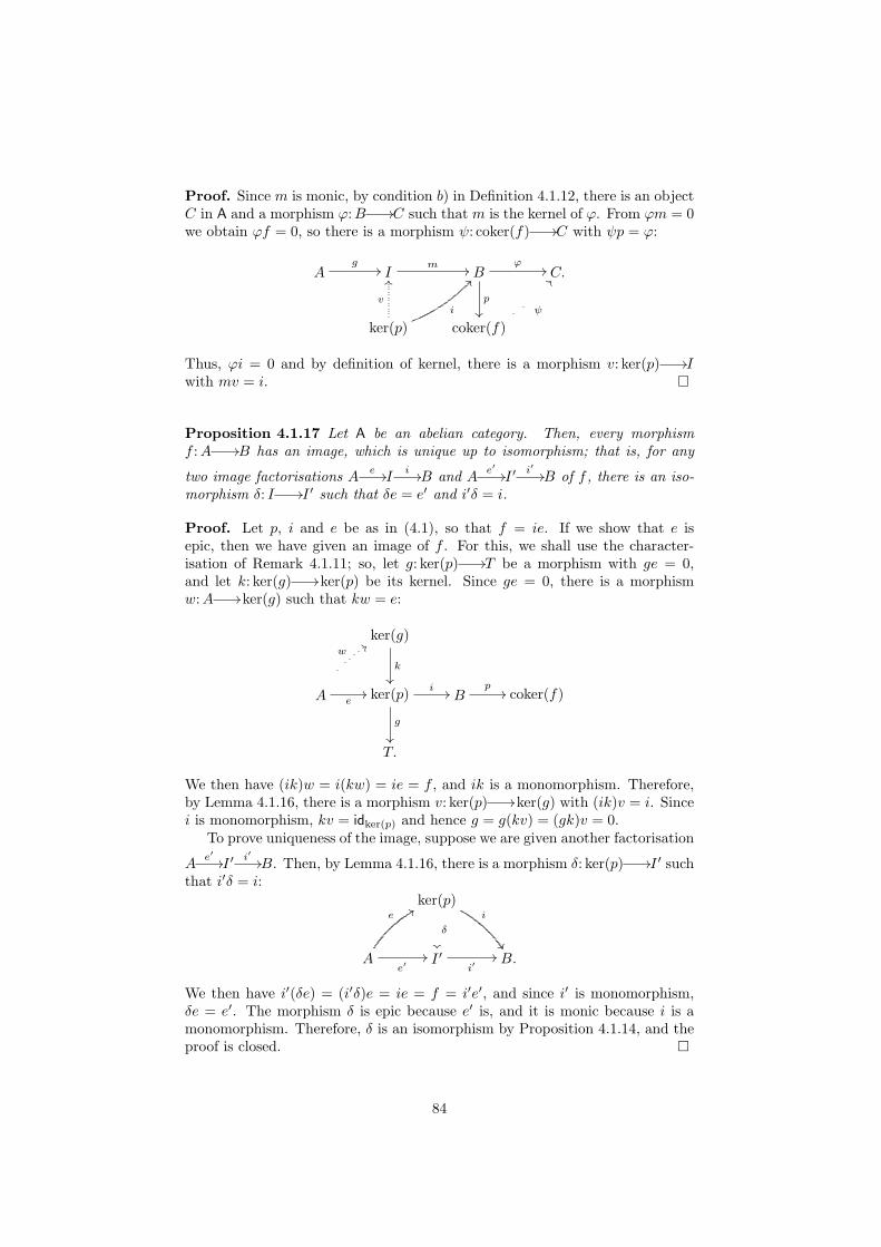
Proof. Since m is monic, by condition b) in Definition 4.1.12, there is an objectC in A and a morphism ϕ:B //C such that m is the kernel of ϕ. From ϕm = 0we obtain ϕf = 0, so there is a morphism ψ: coker(f) //C with ψp = ϕ:

Ag

// Im // B

p

²²

ϕ// C.

ker(p)

v

OO

i

@@

coker(f)ψ

BB

Thus, ϕi = 0 and by definition of kernel, there is a morphism v: ker(p) //Iwith mv = i. ¤

Proposition 4.1.17 Let A be an abelian category. Then, every morphismf :A //B has an image, which is unique up to isomorphism; that is, for any

two image factorisations A e //Ii //B and A e′ //I ′ i′ //B of f , there is an iso-

morphism δ: I //I ′ such that δe = e′ and i′δ = i.

Proof. Let p, i and e be as in (4.1), so that f = ie. If we show that e isepic, then we have given an image of f . For this, we shall use the character-isation of Remark 4.1.11; so, let g: ker(p) //T be a morphism with ge = 0,and let k: ker(g) // ker(p) be its kernel. Since ge = 0, there is a morphismw:A // ker(g) such that kw = e:

ker(g)

k

²²

A

w88

e// ker(p)

g

²²

i // Bp

// coker(f)

T.

We then have (ik)w = i(kw) = ie = f , and ik is a monomorphism. Therefore,by Lemma 4.1.16, there is a morphism v: ker(p) // ker(g) with (ik)v = i. Sincei is monomorphism, kv = idker(p) and hence g = g(kv) = (gk)v = 0.

To prove uniqueness of the image, suppose we are given another factorisation

Ae′ //I ′ i′ //B. Then, by Lemma 4.1.16, there is a morphism δ: ker(p) //I ′ such

that i′δ = i:ker(p)

i

½½

δ

²²

A

e88

e′// I ′

i′// B.

We then have i′(δe) = (i′δ)e = ie = f = i′e′, and since i′ is monomorphism,δe = e′. The morphism δ is epic because e′ is, and it is monic because i is amonomorphism. Therefore, δ is an isomorphism by Proposition 4.1.14, and theproof is closed. ¤

84

Having recovered the notion of kernel, image and zero map, we can now re-formulate in any abelian category the definition of an exact sequence. Formally,this is the same as Definition 1.6.2. So, we shall say that a (possibly infinite)sequence

· · · // Ai+1φi+1

// Aiφi // Ai−1

// · · ·of objects and maps in an abelian category A is exact at Ai if ker(φi) = im(φi+1),and that it is exact if it is exact at Ai for all i. Likewise, a short exact sequencewill be an exact sequence of the special form

0 // A′φ

// Aψ

// A′′ // 0.

The notions of left exact, right exact and exact functor as introduced in Definition1.6.9 readily translate in the present context, for any additive functor betweenabelian categories. Notice that the notion of exactness is self-dual, in the sensethat a sequence in A is exact if and only if the same sequence is exact in Aop.

Many arguments which we saw in Chapter 1 can be recovered in this moregeneral context, just by chasing arrows in a diagram, instead of elements.

Example 4.1.18 Just as for categories of modules, we can characterise mono-and epimorphisms in terms of exact sequences, in any abelian category:

a) the sequence 0 //Aϕ

//B is exact if and only if ϕ is monic;

b) the sequence Aϕ

//B //0 is exact if and only if ϕ is epic.

Example 4.1.19 If T is any object in an abelian category A, then the functorsHomA(T,−): A //Ab and HomA(−, T ): Aop //Ab are left exact.

The contravariant Hom functor is also useful in detecting exactness of se-quences, as made precise by the following result.

Lemma 4.1.20 If a sequence Af

//Bg

//C in an abelian category A has theproperty that for every object T , HomA(−, T ) sends it to the exact sequence

HomA(C, T )g∗

// HomA(B, T )f∗

// HomA(A, T )

of abelian groups, then the sequence is itself exact.

Proof. Take T = C, then the sequence

HomA(C,C)g∗

// HomA(B,C)f∗

// HomA(A,C)

is exact, so f∗g∗ = 0 and hence gf = 0, because gf = f∗g∗(idC). Therefore,im(f) ⊆ ker(g) as subobjects of B, i.e. the inclusion of im(f) in B factorsthrough the monomorphism j: ker(g) //B. For the opposite inclusion, takeT = coker(f). This determines an exact sequence

HomA(C, coker(f))g∗

// HomA(B, coker(f))f∗

// HomA(A, coker(f));

85

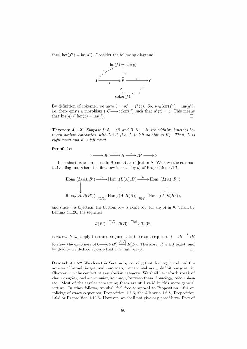
thus, ker(f∗) = im(g∗). Consider the following diagram:

im(f) = ker(p)

i

²²

Af

//

e66

Bg

//

p

²²

C

tvv

coker(f).

By definition of cokernel, we have 0 = pf = f∗(p). So, p ∈ ker(f∗) = im(g∗),i.e. there exists a morphism t:C // coker(f) such that g∗(t) = p. This meansthat ker(g) ⊆ ker(p) = im(f). ¤

Theorem 4.1.21 Suppose L:A //B and R:B //A are additive functors be-tween abelian categories, with LaR (i.e. L is left adjoint to R). Then, L isright exact and R is left exact.

Proof. Let

0 // B′f

// Bg

// B′′ // 0

be a short exact sequence in B and A an object in A. We have the commu-tative diagram, where the first row is exact by b) of Proposition 4.1.7:

HomB(L(A), B′)f∗ //

τ

²²

HomB(L(A), B)g∗ //

τ

²²

HomB(L(A), B′′)

τ

²²

HomA(A,R(B′))R(f)∗

// HomA(A,R(B))R(g)∗

// HomA(A,R(B′′)),

and since τ is bijection, the bottom row is exact too, for any A in A. Then, byLemma 4.1.20, the sequence

R(B′)R(f)

// R(B)R(g)

// R(B′′)

is exact. Now, apply the same argument to the exact sequence 0 //B′f

//B

to show the exactness of 0 //R(B′)R(f)

// R(B). Therefore, R is left exact, andby duality we deduce at once that L is right exact. ¤

Remark 4.1.22 We close this Section by noticing that, having introduced thenotions of kernel, image, and zero map, we can read many definitions given inChapter 1 in the context of any abelian category. We shall henceforth speak ofchain complex, cochain complex, homotopy between them, homology, cohomologyetc. Most of the results concerning them are still valid in this more generalsetting. In what follows, we shall feel free to appeal to Proposition 1.6.4 onsplicing of exact sequences, Proposition 1.6.6, the 5-lemma 1.6.8, Proposition1.9.8 or Proposition 1.10.6. However, we shall not give any proof here. Part of

86

the motivation for this choice is that the arguments are easy formal adaptationsof the original proofs in the case of modules (see exercise h) below). Moreover,such proofs are made unnecessary by Freyd’s embedding theorem [1, 5], to whichwe refer any interested reader.

Exercises

a) Prove the properties of linear categories expressed in Proposition 4.1.5.b) Prove the properties of kernel and cokernel maps stated in Proposition

4.1.7.c) Prove Proposition 4.1.10.d) Prove Proposition 4.1.14.e) Prove a) and b) of Example 4.1.18.f) Show functoriality and exactness of the Hom functors in Example 4.1.19.g) Show that any abelian category A admits pullbacks, i.e. that, for any

diagram of the formB

f

²²

A g// C

in A, there exists an object P and maps i and j fitting in a commutativesquare

Pi //

j

²²

B

f

²²

A g// C,

with the universal property that, for any other pair of maps j′:X //Aand i′:X //B with fi′ = gj′, there is a unique morphism e:X //P suchthat je = j′ and ie = i′. (Hint: build P as the kernel of an appropriatemap from A⊕B to C.)

h) In light of Remark 4.1.22, give a categorical proof of some of the resultsin Chapter 1 concerning exact sequences and (co)homology, such as the5-lemma or Proposition 1.10.6.

4.2 Derived functors

In this Section, we shall study the notion of derived functors. Given a leftexact functor F : A //X between abelian categories, and a short exact sequence0 //A //B //C //0 in A, we know that there is an exact sequence

0 // FA // FB // FC, (4.2)

but the rightmost map need not be an epimorphism. The right derived functorsof F provide a suitable extension of (4.2) to a long exact sequence. Left derivedfunctors provide the dual extension for right exact functors.

We shall henceforth assume all functors to be additive.

87

4.2.1 Left derived functors

As made clear in Remark 4.1.22, most notions introduced for modules in Chapter1 can be formulated in any abelian category. This is the case also for the notionof a projective module (Definition 1.7.1).

Definition 4.2.1 An object P in an abelian category A is projective if thefunctor HomA(P,−): A //Ab is (right) exact. Equivalently, P is projective if,for any epimorphism f :A //B, every map g:P //B factors through f :

A

f²²²²

P

66

g// B.

We say that A has enough projectives if every A in C can be covered by aprojective; that is, if there exists an epimorphism f :P //A, where P is aprojective object.

Example 4.2.2 For any ring R, the category R-mod of left R-modules hasenough projectives, by Lemma 1.7.5.

Remark 4.2.3 The arguments given for Lemma 1.10.12 and Proposition 1.10.13readily extend to any abelian category A, showing that if A has enough projec-tives, then every object admits a projective resolution, which is unique up tohomotopy of chain complexes.

Definition 4.2.4 Let A and X be abelian categories such that A has enoughprojectives. Let F : A //X be a right exact functor. Then, the left derivedfunctors of F are the functors Li(F ): A //X (i ∈ N) which, for an object A inA with a projective resolution 0 Aoo P?oo , are defined as

Li(F )(A) = Hi(F (P?)) for i ≥ 0.

Given a morphism f :A //B in A, where 0 Aoo P?oo and 0 Boo Q?oo

are two projective resolutions of A and B, respectively, there exists a (unique,up to homotopy) chain complex map f?:P? //Q? which extends f . The actionof the derived functor Li(F ) on f is then defined as

Li(F )(f) = Hi(F (f?)). (i ≥ 0)

Remark 4.2.5 The next proposition will make the properties of left derivedfunctors clear. However, before moving forward, we have to understand whatwe mean by homology group in Definition 4.2.4. Given a chain complex A? inan abelian category A, the condition dd = 0 implies that, for every i ∈ N, thereexists a monomorphism im(di+1) // ker(di). The i-th homology group Hi(A?)of A? is defined as the cokernel of this monomorphism.

Proposition 4.2.6 Let A be an abelian category with enough projectives and Fa right exact functor. Then:

88

a) the object Li(F )(A) is independent (up to a canonical isomorphism) ofthe projective resolution P? of A, and the image along Li(F )(−) of a mapf :A //B is independent of the chain map f? lifting f . Moreover, Li(F )(−)is a covariant functor;b) for any A in A, we have L0(F )(A) ∼= FA. More precisely there is anatural isomorphism L0(F ) ∼= F ;c) any short exact sequence in A

0 //Af

//Bg

//C //0

gives rise to a long exact sequence in X

· · · //L1(F )(C) δ //L0(F )(A) //L0(F )(B) //L0(F )(C) //0;

d) If A is projective in A, then Li(F )(A) = 0 for i > 0.

Proof. a) Consider a morphism f :A //B in A, and suppose two projectiveresolutions P? → A and Q? → B are given. Then, by Lemma 1.10.12 we knowthat f lifts to a morphism of exact sequences f?:P? //Q?. Moreover, f? isunique up to homotopy. Therefore, it induces a unique map in homology:

Hi(F (f?)):Hi(F (P?)) //Hi(F (Q?)).

This shows that the action of Li(F ) on maps is well-defined. Moreover, bytaking f = idA, we show that, up to isomorphism, Li(F )(A) = Hi(F (P?)) doesnot depend on the choice of the projective resolution P? of A. Functoriality nowfollows immediately.

b) Let A P?oo be a projective resolution of A. Then, by right exactness of

F , we get the exact sequence F (P1)F (d1)

// F (P0)F (d0)

// F (A) //0, showing thatF (A) ∼= coker(F (d1)). However, we know by the definition of the left derivedfunctor that L0(F )(A) = H0(F (P?)) = coker(F (d1)), hence L0(F )(A) ∼= F (A).

c) By Lemma 4.2.7 below, we can derive projective resolutions P?, Q? andR? for A, B and C, respectively, with the sequence 0 //P? //Q? //R? //0exact and pointwise split. Since additive functors preserve split exact sequences,it follows that 0 //F (P?) //F (Q?) //F (R?) //0 is also exact (and pointwisesplit). Hence, by Proposition 1.9.8, there is a long exact sequence in homology:

· · · // H1(F (R?))δ // H0(F (P?)) // H0(F (Q?)) // H0(F (R?)) // 0.

d) If A is a projective object, then 0 // AidA // A // 0 is a projective res-

olution of A; so, this part of the statement follows immediately from a). ¤

Lemma 4.2.7 Let 0 //Af

//Bg

//C //0 be a short exact sequence in an

abelian category A, and suppose A P?doo and C R?

loo are two projectiveresolutions of A and C, respectively. Then, there is a projective resolution

B Q?eoo and two chain maps f?:P? //Q? and g?:Q? //R? (lifting f and

g, respectively), such that the following sequence is exact and poinwise split:

0 // P?f? // Q?

g? // R? // 0. (4.3)

89

Proof. Since g:B //C is epic and R0 is projective, there exists a morphismα:R0

//B such that gα = l. Consider the direct sum Q0 = P0⊕R0, withinjections i and j, and projections p and q from and to P0 and R0, respectively.Then, the composite fd and the map α determine, via the universal propertyof Q0, a unique map e:Q0

//B such that ei = fd and ej = α:

0 // Af

//// Bg

// C // 0

0 // P0i //

d

OO

P0 ⊕R0

q//

e

OO

R0j

oo //

l

OO

α

ddIIIIIIIIII0.

(4.4)

We have ge = ge(idQ0) = (ge)(ip + jq) = g(ei)p + g(ej)q = gfd + (gα)q = lq;moreover, the map e is epic. To see this, suppose h:B //E is a morphismsuch that he = 0; we then have 0 = hei = hfd, and hf = 0, because d is anepimorphism. Therefore, h factors through a map y:C //E, so that yg = h,and we have 0 = he = yge = ylq. Since l and q are epic, we get y = 0, andtherefore h = 0.

Now, form the kernel of the maps d, e and l, with inclusions i1, i2 and i3,respectively. Then, the maps i and q restrict to maps i′ and q′, which form thesequence

0 // ker(d) i′ // ker(e)q′

// ker(l) // 0. (4.5)

The map i′ is clearly monic, since i and i1 are. Moreover, q′ is epic. To seethis, notice first that there is an obvious epimorphism l′:R1

// ker(l). Then,we have geji3l′ = 0, hence the composite eji3l′ factors as fγ, for some mapγ:R1

//A, and because R1 is projective, this factors in turn as γ = dβ, fora map β:R1

//P0. Now, consider the map φ = ji3l′ − iβ. We have that

qφ = qji3l′− qiβ = i3l

′; also, eφ = eji3l′− eiβ = eji3l

′−fdβ = eji3l′−fγ = 0,

hence φ = i2ψ, for some ψ:R1// ker(e). Therefore, i3q′ψ = qi2ψ = qφ = i3l

′,and since i3 is monic, we have l′ = q′ψ. This shows that q′ is epic, because l′

is. This proves exactness of (4.5) at ker(d) and ker(l).To prove that it is exact also at ker(e), notice that i3q′i′ = qi2i

′ = qii1 = 0,and because i3 is monic, q′i′ = 0, which implies im(i′) ⊆ ker(q′). Conversely,given a map h:X //Q0 such that eh = 0 (i.e. h factors through ker(e)) andqh = 0, we have h = idQ0h = (ip + jq)h = iph, hence fdph = eiph = eh = 0.Because f is monic, we get that dph = 0, so we have factored h through i via ph,which in turn factors through ker(d). This shows that ker(q′) ⊆ im(i′), hence(4.5) is an exact sequence. We then have the following diagram in which d′, l′

are epimorphisms and the map e′ is determined in the same way as the map ein (4.4) above:

0 // P0i // P0 ⊕R0

q// R0

// 0

0 // ker(d)

i1

OO

i′ // ker(e)

i2

OO

q′// ker(l)

i3

OO

// 0

0 // P1

d′

OO

i// P1 ⊕R1

e′

OO

q// R1

l′

OO

// 0.

90

We now set Q1 = P1⊕R1 and e = i2e′, and proceed by induction in defining the

objects Qi = Pi⊕Ri and the morphism e. It is clear by construction that thechain complex B Q?oo is a projective resolution of B, and the maps i and qform a pointwise split exact sequence. ¤

Remark 4.2.8 Notice that the sequence (4.3) in the previous statement is ashort exact sequence of chain complexes, which is pointwise split. However, thisdoes not mean that it is itself a split sequence of chain complexes.

Definition 4.2.9 Let A and X be abelian categories. A (homological) δ-functoris a sequence of functors Gn: A //X (n ≥ 0) such that, for any short exactsequence 0 //A //B //C //0, there exist morhisms δ:Gn(C) //Gn−1(A)(n ≥ 0) which satisfy the following properties:

a) there is a long exact sequence

· · · //G1(C) δ //G0(A) //G0(B) //G0(C) //0;

b) the morphisms δ are natural; that is, for any commutative diagram

0 // A //

²²

B //

²²

C //

²²

0

0 // A′ // B′ // C ′ // 0

of short exact sequences, the following diagram is commutative for all n > 0:

Gn(C) δ //

²²

Gn−1(A)

²²

Gn(C ′)δ′

// Gn−1(A′).

Example 4.2.10 For any right exact functor F : A //X, the derived functorsand the connecting morphism described in Proposition 4.2.6 c) form a (homo-logical) δ-functor (Li(F ), δ).

Definition 4.2.11 A morphism φ: (G, δ) //(G′, δ′) between δ-functors is a se-quence of natural transformations φn:Gn //G′n which are compatible with δ’s,that is, for any short exact sequence 0 //A //B //C //0, the followingsquare commutes:

Gn(C) δ //

φn

²²

Gn−1(A)

φn−1

²²

G′n(C)δ′

// G′n−1(A).

Now, we are ready to give a universal characterisation of left derived functors.

Theorem 4.2.12 (Universal property of left derived functors) Let F bea right exact functor A //X between abelian categories, where A has enoughprojectives, and let (G, δ′): A //X be a (homological) δ-functor. Then:

91

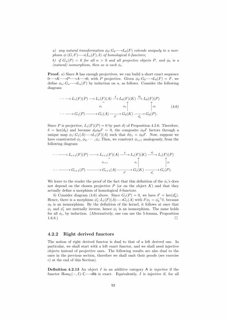
a) any natural transformation φ0:G0//L0(F ) extends uniquely to a mor-

phism φ: (G, δ′) //(L?(F ), δ) of homological δ-functors;b) if Gn(P ) = 0 for all n > 0 and all projective objects P , and φ0 is a(natural) isomorphism, then so is each φi.

Proof. a) Since A has enough projectives, we can build a short exact sequence0 //K //P //A //0, with P projective. Given φ0:G0

//L0(F ) = F , wedefine φn:Gn //Ln(F ) by induction on n, as follows. Consider the followingdiagram:

· · · // L1(F )(P ) // L1(F )(A) δ // L0(F )(K)d0 // L0(F )(P )

· · · // G1(P ) // G1(A)

φ1

OO

δ′// G0(K)

d′0

//

φ0

OO

G0(P ).

φ0

OO

(4.6)

Since P is projective, L1(F )(P ) = 0 by part d) of Proposition 4.2.6. Therefore,δ = ker(d0) and because d0φ0δ

′ = 0, the composite φ0δ′ factors through a

unique map φ1:G1(A) //L1(F )(A) such that δφ1 = φ0δ′. Now, suppose we

have constructed φ1, φ2, · · · , φi; Then, we construct φi+1 analogously, from thefollowing diagram:

· · · // Li+1(F )(P ) // Li+1(F )(A) δ // Li(F )(K)di // Li(F )(P )

· · · // Gi+1(P ) // Gi+1(A)

φi+1

OO

δ′// Gi(K)

d′i

//

φi

OO

Gi(P ).

φi

OO

We leave to the reader the proof of the fact that this definition of the φi’s doesnot depend on the chosen projective P (or on the object K) and that theyactually define a morphism of homological δ-functors.

b) Consider diagram (4.6) above. Since G1(P ) = 0, we have δ′ = ker(d′0).Hence, there is a morphism φ′1:L1(F )(A) //G1(A) with δ′φ1 = φ−1

0 δ, becauseφ0 is an isomorphism. By the definition of the kernel, it follows at once thatφ1 and φ′1 are mutually inverse, hence φ1 is an isomorphism. The same holdsfor all φi, by induction. (Alternatively, one can use the 5-lemma, Proposition1.6.8.) ¤

4.2.2 Right derived functors

The notion of right derived functor is dual to that of a left derived one. Inparticular, we shall start with a left exact functor, and we shall need injectiveobjects instead of projective ones. The following results are also dual to theones in the previous section, therefore we shall omit their proofs (see exercisec) at the end of this Section).

Definition 4.2.13 An object I in an additive category A is injective if thefunctor HomC(−, I): C //Ab is exact. Equivalently, I is injective if, for all

92

monomorphisms f :A //B and maps g:A //I there is an extension of g alongf :

Ag

//

f

²²

I.

B

GG

We say that A has enough injectives if, for any object A in A, there exists amonomorphism f :A //I, where I is an injective object.

Definition 4.2.14 (Dual of Definition 4.2.4) Let A and X be abelian cate-gories such that A has enough injectives. Let F : A //X be a left exact functor.Then, the right derived functors of F are the functors Ri(F ): A //X (i ∈ N)which, for an object A in A with an injective resolution 0 //A //I?, are de-fined as

Ri(F )(A) = Hi(F (I?)) for i ≥ 0.

Given a morphism f :A //B in A, where 0 //A //I? and 0 //B //J? aretwo injective resolutions of A and B, respectively, there exists a (unique, up tohomotopy) chain complex map f?: I? //J? which extends f . The action of thederived functor Ri(F ) on f is then defined as

Ri(F )(f) = Hi(F (f?)).

Lemma 4.2.15 (Dual of Lemma 4.2.7) Let 0 // Af

// Bg

// C // 0 bea short exact sequence in an additive category A. Suppose A //I? and C //K?

are two injective resolutions of A and C, respectively. Then, there is an injec-tive resolution B //J? and two chain maps f?: I? //J? and g?: J? //K?

such that the sequence

0 // I?f?

// J?g?

// K? // 0

is exact and pointwise split.

Proposition 4.2.16 (Dual of Proposition 4.2.6) Let A be an abelian cate-gory with enough injectives and F a left exact functor. Then:

a) the object Ri(F )(A) is independent of the injective resolution I? of A,and the image along Ri(F )(−) of a map f :A //B is independent of thechain map f? lifting f . Moreover, Ri(F )(−) is a covariant functor;b) for any A in A, we have R0(F )(A) ∼= FA. More precisely there is anatural isomorphism R0(F ) ∼= F ;c) any short exact sequence in A

0 //Af

//Bg

//C //0

gives rise to a long exact sequence in X

0 //R0(F )(A) //R0(F )(B) //R0(F )(C) δ //R1(F )(A) // · · · ;

d) if A is injective in A, then Ri(F )(A) = 0 for i > 0.

93

Definition 4.2.17 A (cohomological) δ-functor between abelian categories Aand X is a sequence of functors Gn: A //X (n > 0) such that for any short exactsequence 0 //A //B //C //0, there exist morphisms δ:Gn(C) //Gn+1(A)satisfying the following properties:

a) there is a long exact sequence

0 //G0(A) //G0(B) //G0(C) δ //G1(A) // · · · ;

b) the morphism δ is natural; that is, for any commutative diagram

0 // A //

²²

B //

²²

C //

²²

0

0 // A′ // B′ // C ′ // 0

of short exact sequences, the following square commutes for all n > 0:

Gn(C) δ //

²²

Gn+1(A)

²²

Gn(C ′)δ′

// Gn+1(A′).

Example 4.2.18 For any left exact functor F : A //X, the right derived func-tors and the connecting morphisms of Proposition 4.2.16 c) form a (cohomolog-ical) δ-functor (Ri(F ), δ).

Definition 4.2.19 Let (G, δ) and (G′, δ′) be two (cohomological) δ-functors. Amorphism φ: (G, δ) //(G′, δ′) consists of a sequence of natural transformationsφn:Gn //G′n which are compatible with δ’s; that is, for every short exactsequence 0 //A //B //C //0, the following commutes:

Gn(C) δ //

φn

²²

Gn+1(A)

φn+1

²²

G′n(C)δ′

// G′n+1(A).

Theorem 4.2.20 (Universal property of right derived functors) Let Fbe a left exact functor A //X between abelian categories, where A has enoughinjectives, and (G, δ′): A //X a (cohomological) δ-functor. Then:

a) any natural transformation φ0:R0(F ) //G0 extends uniquely to a mor-phism φ: (R?(F ), δ) //(G, δ′) of cohomological δ-functors;b) if Gn(I) = 0 for all n > 0 and all injective objects I, and φ0 is a (natural)isomorphism, then so is each φi.

Exercises

a) Give an argument for the statement of Remark 4.2.3.

94

b) Reformulate Theorem 4.2.12 a) in terms of an adjunction between thecategory of right exact functors from A to X and that of homologicalδ-functors between the same categories.

c) Check that the definition and results of Section 4.2.2 are reformulationsof those of Section 4.2.1 for the dual category Aop, hence do not need tobe proved again.

d) Reformulate Theorem 4.2.20 a) in terms of an adjunction between thecategory of left exact functors from A to X and that of cohomologicalδ-functors between the same categories.

4.3 Cohomology of Small Categories

In this Section, we shall apply the machinery of derived functors to the studyof cohomology of small categories. Starting with a fixed small category C,we shall associate an abelian category Ab(C) to it, and a left exact functorΓ:Ab(C) //Ab. The right derived functors RnΓ will then describe the coho-mology of C, as obtained from its nerve.

So, we start by defining the category Ab(C) of presheaves of abelian groups onC. This is the functor category [Cop,Ab], whose objects are contravariant func-tors from C to Ab and whose arrows are natural transformations (see RemarkA.0.13 in the Appendix).

For an arrow u:C //D in C and a presheaf A: Cop //Ab in Ab(C), the arrowA(u):A(D) //A(C) will be sometimes denoted by u∗. Recall that the natural-ity condition in the definition of morphisms in Ab(C) reads as commutativity ofthe following diagram:

A(D)A(u)

//

fD

²²

A(C)

fC

²²

B(D)B(u)

// B(C).

For every object C in C, there is an evaluation functor evC : Ab(C) //Ab, de-fined on a presheaf A as evC(A) = A(C), and on a presheaf morphism f :A //Bas evC(f) = fC .

Example 4.3.1

a) Consider a group G as a category G with just one object ? and one arrowg: ?→ ? for every element g ∈ G. Then, Ab(G) = mod-G = mod-Z[G];b) Consider the category ∆, whose objects are ordered initial segments ofthe natural numbers [n] = 0, 1, ..., n, n ≥ 0, and arrows are non decreasingfunctions. Then, Ab(∆) is the abelian category of simplicial abelian groups.c) Let X be a topological space with a basis B of open sets. View B as acategory whose arrows are inclusions. Many “geometric structures” on Xgive rise to objects of Ab(B); for example, if E //X is a vector bundle, thenthere is a functor Γ(E) in Ab(B), where Γ(E)(U) = Γ(U,E), the sections ofE|U , for U ∈ B.

Proposition 4.3.2 Let C be a small category. Then:

95

a) Ab(C) is an abelian category;b) for each C in C, evC is an exact functor;c) Ab(C) has enough projectives.

The category Ab(C) also has enough injectives, but we will not prove this here.

Proof. In order to prove a) we need to construct finite direct sums, kernelsand cokernels of functors. We do this pointwise; for example, if A and Bare presheaves in Ab(C), put (A ⊕ B)(C):= A(C) ⊕ B(C), for a morphismf :A //B in Ab(C), put (ker f)(C):= ker(A(C) //B(C)) and so on. Wemay take these as a definition and check that they have the required uni-versal properties. As an illustration, we derive the existence of cokernels:let (coker f)(C):= coker(A(C) //B(C)) and, for an arrow u:C //D in C,(coker f)(u) is the unique arrow coker f(D) // coker f(C) making the follow-ing commute:

A(D)

A(u)

²²

fD // B(D)

B(u)

²²

PD // (coker f)(D)

²²

A(C)fC

// B(C)PC

// (coker f)(C).

(4.7)

The mappings C 7→ (coker f)(C) and u 7→ (coker f)(u) determine a contravari-ant functor from C to Ab, i.e. an object in Ab(C), which we denote by coker f .Moreover, the collection of maps PC (C in C) form a natural transformation;that is, an arrow in Ab(C). It is immediate from (4.7) that the object coker fand the arrow P form the cokernel of f in Ab(C).

It is now immediate that b) holds, since we just saw that kernels and cokernelsin Ab(C) are computed pointwise.

The proof of c) goes via a reduction to the category of sets. First of all, noticethat, similarly to the definition of Ab(C), we may define Set(C) as the category ofcontravariant functors S:Cop //Set and natural transformations between them.As before, we have for each C in C an evaluation functor evC : Set(C) //Set.The important category of simplicial sets is of this type: it is the categorySet(∆). Now, we need a couple of results.

Lemma 4.3.3 An arrow f :S //T in Set(C) is an epimorphism if and only iffC :S(C) //T (C) is surjective for all C in C.

Proof. See Exercise a) below. ¤

Now, notice that there is an obvious adjunction Z[−]aU between the for-getful functor U :Ab //Set and the free abelian group functor Z[−]: Set //Ab.Composition with these two functors induces an adjunction

Ab(C)U //> Set(C),Z[−]

oo (4.8)

where, by an abuse of notation, we denote again by U the functor which point-wise forgets the abelian group structure, and by Z[−] the functor which point-wise takes the free abelian group; in other words, Z[S](C) = Z[S(C)] for anyfunctor S: Cop //Set and any C in C.

From Lemma 4.3.3, it then follows (see Exercise b) below) that:

96

Remark 4.3.4

a) For any A in Ab(C), the A-th component of the counit

εA:Z[U(A)] //A

is epic;b) by the dual of Lemma 1.8.12, since Z[−] is left-adjoint to U and the latterclearly preserves epimorphisms, Z[−] preserves projectives;c) if P //S is an epimorphism in Set(C), then Z[P ] //Z[S] is epic in Ab(C)(see exercise e) in the Appendix).

Now, in order to prove that Ab(C) has enough projectives, it is enoughto show that Set(C) does; for, if this is the case, then, given any presheafA:Cop //Ab, we can cover its image U(A) in Set(C) with a projective P , andthen, by Remark 4.3.4, the composite

Z[P ] // Z[U(A)] ε // A

is a covering of A by an epimorphism from the projective Z[P ].To show that Set(C) has enough projectives, recall from the Appendix the

notion of representable functor in Set(C) and Yoneda’s lemma A.0.15. Then,the following result closes the proof of Proposition 4.3.2. ¤

Proposition 4.3.5 For a small category C:

a) each representable presheaf in Set(C) is projective;b) Set(C) has enough projectives.

Proof.

a) Let B in C and consider the diagram in Set(C)

T

g

²²

HomC(−, B)f

// S,

where g is an epimorphism. Then, by Yoneda’s Lemma, a natural trans-formation HomC(−, B) //T corresponds to an element of T (B). Since gBis surjective, we may take any element in the preimage of fB(idB).

b) Let S in Set(C) and consider the coproduct P =∐B∈C,s∈S(B) HomC(−, B).

Then, by a) P is projective in Set(C). For each B in C and s ∈ S(B),Yoneda’s Lemma gives an arrow HomC(−, B) //S, so by the universalproperty of coproducts we obtain an arrow P //S, which is epic by Lemma4.3.3.

¤

97

Now that we have established the fact that Ab(C) is an abelian categoryand has enough projectives, we can turn our attention to describing a left exactfunctor from Ab(C) to Ab.

This will be the functor Γ: = HomAb(C)(Z,−): Ab(C) //Ab, where Z is theconstant functor mapping every object of C to Z.

Recall that, for every abelian group B, we have HomAb(Z, B) ' B; there-fore, for A in Ab(C) and a natural transformation α in HomAb(C)(Z, A), we canidentify the C-th component of α (for C in C) with an element in A(C). It fol-lows that Γ(A) is the set of functions α (also called sections) assigning to eachobject C ∈ C an element α(C) ∈ A(C) such that, for each arrow u:D //C,u∗(α(C)) = α(D).

Remark 4.3.6 The functor Γ has a left adjoint K: Ab //Ab(C), sending anabelian group to the corresponding constant presheaf. In particular, by Theorem4.1.21, Γ is left exact.

Example 4.3.7 Looking back at Example 4.3.1, we have:

a) When G is the category associated to a group G, we recover (−)G asΓ; indeed, we have already seen in Example 4.3.1 a) that Ab(G) = G-mod.Moreover, the functor K above is just the trivial module functor. Hence, byexercise b) of Section 2.4 and uniqueness of adjoints, (−)G and Γ are naturallyisomorphic;b) for C = ∆, we see that Γ(A) ' A([0]) = A0 (the set of vertices).

4.3.1 The nerve of a category

Our next goal is to give an explicit description of RnΓ, the right derived functorsof Γ. To this end, we recall from Example 3.1.3 b) that the nerve of a (small)category C is the simplicial set N?(C) defined as N0(C) = |C| and for n ≥ 1 asNn(C) = C0

u1←− · · · un←−− Cn, with maps di:Nn(C) //Nn−1(C) which “omitCi”; that is:

di(C0u1←− · · · un←−− Cn) =

C1u2←− · · · un←−− Cn, i = 0

C0 ← · · ·Ci−1uiui+1←−−−− Ci+1 · · · ← Cn, 0 < i < n

C0u1←− · · · un−1←−−− Cn−1, i = n

The di’s satisfy the simplicial identities didj+1 = djdi, for i ≤ j.For a presheaf A in Ab(C), we can build a cochain complex C?(C, A) using

the nerve N?(C), by putting

Cn(C, A):=∏

C0u1←−··· un←−−Cn

A(Cn),

with boundary maps

d =n∑

i=0

(−1)iδi:Cn−1(C, A) //Cn(C, A),

where δi is defined on a tuple α = aC0

u1←−··· un−1←−−−Cn−1

∈ Cn−1(C, A) as

δi(α)C0

u1←−··· un←−−Cn

=

adi(C0

u1←−··· un←−−Cn), i < n

u∗n(adn(C0u1←−··· un←−−Cn)

), i = n.

98

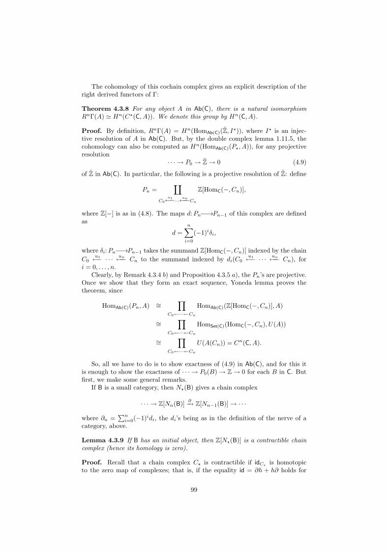
The cohomology of this cochain complex gives an explicit description of theright derived functors of Γ:

Theorem 4.3.8 For any object A in Ab(C), there is a natural isomorphismRnΓ(A) ' Hn(C?(C, A)). We denote this group by Hn(C, A).

Proof. By definition, RnΓ(A) = Hn(HomAb(C)(Z, I?)), where I? is an injec-tive resolution of A in Ab(C). But, by the double complex lemma 1.11.5, thecohomology can also be computed as Hn(HomAb(C)(P?, A)), for any projectiveresolution

· · · → P0 → Z→ 0 (4.9)

of Z in Ab(C). In particular, the following is a projective resolution of Z: define

Pn =∐

C0u1←−··· un←−−Cn

Z[HomC(−, Cn)],

where Z[−] is as in (4.8). The maps d:Pn //Pn−1 of this complex are definedas

d =n∑

i=0

(−1)iδi,

where δi:Pn //Pn−1 takes the summand Z[HomC(−, Cn)] indexed by the chainC0

u1←− · · · un←−− Cn to the summand indexed by di(C0u1←− · · · un←−− Cn), for

i = 0, . . . , n.Clearly, by Remark 4.3.4 b) and Proposition 4.3.5 a), the Pn’s are projective.

Once we show that they form an exact sequence, Yoneda lemma proves thetheorem, since

HomAb(C)(Pn, A) ∼=∏

C0←···←Cn

HomAb(C)(Z[HomC(−, Cn)], A)

∼=∏

C0←···←Cn

HomSet(C)(HomC(−, Cn), U(A))

∼=∏

C0←···←Cn

U(A(Cn)) = Cn(C, A).

So, all we have to do is to show exactness of (4.9) in Ab(C), and for this itis enough to show the exactness of · · · → P0(B)→ Z→ 0 for each B in C. Butfirst, we make some general remarks.

If B is a small category, then N?(B) gives a chain complex

· · · → Z[Nn(B)] ∂−→ Z[Nn−1(B)]→ · · ·

where ∂n =∑ni=0(−1)idi, the di’s being as in the definition of the nerve of a

category, above.

Lemma 4.3.9 If B has an initial object, then Z[N?(B)] is a contractible chaincomplex (hence its homology is zero).

Proof. Recall that a chain complex C? is contractible if idC? is homotopicto the zero map of complexes; that is, if the equality id = ∂h + h∂ holds for

99

opportune maps hn:Z[Nn−1(B)] //Z[Nn(B)]. Let I be the initial object of B.Then, the maps defined by

hn(C0 ← · · · ← Cn−1) = (−1)n(C0 ← · · · ← Cn−1 ← I)

satisfy the condition dihn+1 = −hndi for i = 0, . . . , n and dnhn = (−1)nid.Therefore, id = ∂h+ h∂. ¤

Now, fix an object B in C. The slice category B/C has as objects all pairs(u,C) with C in C and u:B //C, and as arrows f : (u,C) //(v, C ′) all thosearrows f :C //C ′ for which fu = v. The definition of arrows in B/C allowsus to identify Nn(B/C) with the set Sn of strings C0 ← · · · ← Cn ← B,hence S? is exactly the nerve N?(B/C). Also, the sum of all abelian groupsZ[HomC(B,Cn)], indexed over the strings C0 ← · · · ← Cn, is isomorphic toZ[Sn], hence Pn(B) ∼= Z[Sn]. From this we derive (see Exercise c) below)

Proposition 4.3.10 The complexes P?(B) and Z[N?(B/C)] are isomorphic.

Now, since (idB , B) is an initial object for B/C, Lemma 4.3.9 and Proposition4.3.10 imply the exactness of:

· · · → P1(B)→ P0(B)→ Z→ 0.

This finishes the proof of Theorem 4.3.8. ¤

Exercises

a) For an object C in C, show that the evaluation functor evC :Set(C) //Sethas a right adjoint defined by

RC(S) = HomSet(HomC(C,−), S);

Use this adjunction to prove Lemma 4.3.3.b) Give a proof of a), b) and c) in Remark 4.3.4.c) Prove Proposition 4.3.10 in detail.

4.4 Sheaf cohomology

For a fixed topological space X, we shall construct an abelian category Sh(X)of sheaves on X, together with a left exact functor Γ: Sh(X) //Ab. Then, weshall define the sheaf cohomology of the space X as Hn(X,A) = (RnΓ)(A), forA in Sh(X).

As a starting point, consider the partial order O(X), the set of open sub-sets of X as a small category. We can form the abelian category Ab(O(X))of presheaves of abelian groups on X, just like in Section 4.3. Its objects arecontravariant functors from O(X) to Ab; for an inclusion U ⊆ V of open sub-sets of X, such a presheaf A in Ab(O(X)) determines a map A(V ) //A(U),called a restriction morphism. The image of an element a ∈ A(V ) along such arestriction morphism will be denoted by a|U .

100

Just as in Section 4.3, for any open set U ∈ O(X), there is an exact eval-uation functor evU :Ab(O(X)) //Ab. The definition of the functor Γ standsalso in this context, and one can check that, for any presheaf A in Ab(O(X)),Γ(A) = evX(A) = A(X).

Now, we define Sh(X) as a full subcategory of Ab(O(X)) and, with an abuseof notation, we still write Γ for the restriction Γ: Sh(X) //Ab. It is importantto note that this restriction will not be exact; in particular, the inclusion functori: Sh(X) //Ab(O(X)) is not exact.

Definition 4.4.1 Let A ∈ Ab(O(X)) be a presheaf of abelian groups on X,U ∈ O(X) and consider an open cover Uii∈I of U . A family ai ∈ A(Ui)i∈Iis called compatible if ai|Uij = aj |Uij for all i, j, where Uij = Ui ∩ Uj . Anamalgamation, or glueing, of the family ai is an a ∈ A(U) with a|Ui

= ai forall i.

We say that A is a sheaf if for every open cover Ui of an open U ∈ O(X),every compatible family has a unique amalgamation.

Example 4.4.2 Classical examples of sheaves are:

a) Define R(U):= C0(U,R), the set of continuous functions from U to R,and for U ⊆ V let the map R(V )→ R(U) be the usual restriction of functions.Then, R is a sheaf.b) For any topological abelian group A, we have a similar sheaf A, whereA(U) = C0(U,A). If A has the discrete topology, we also denote the sheafA by K(A), and in this case K(A)(U) is the set of locally constant functionsU → A.c) Let p:E //X be a vector bundle on X. We define a sheaf E by

E(U):= Γ(U,E) = s:U → E | s continuous and ps = id.This construction makes sense for any bundle of abelian groups A→ X.

4.4.1 Germs of functions

Let U be an open subset of X, f :U //R a continuous map and x ∈ U . Thegerm of f at x, germx(f), is the equivalence class of all those functions whosebehaviour in a neighbourhood of x is equal to that of f . More precisely, we definethe set Germ(x) of germs of continuous functions at x as the set of equivalenceclasses of pairs (f, U), where f ∈ C0(U,R) and x ∈ U , modulo the equivalencerelation defined by (f, U) ∼ (g, V ) iff there is W ∈ O(X) with x ∈ W ⊆ U ∩ Vsuch that f |W = g|W .

Using the group structure of R, we can induce on the set Germ(x) an abeliangroup structure, by letting

[(f, U)] + [(f ′, U ′)] = [(f |U∩U ′ + f ′|U∩U ′ , U ∩ U ′)].Categorically, we can present this construction as a colimit: if U is an open

neighbourhood of x, then

Germ(x) = lim−−−→U⊆X

C0(U,R) = lim−−→x∈U

R(U).

In fact, this expression makes sense for any sheaf A:

101

Definition 4.4.3 The stalk of A at the point x ∈ X is the abelian group

Ax = lim−−→x∈U

A(U).

In other words, the elements of Ax are equivalence classes of pairs (a, U), wherex ∈ U and a ∈ A(U), under the relation (a, U) ∼ (b, V ) iff a|W = b|W for someW ∈ O(X) with x ∈W ⊂ U ∩ V . These classes add up as:

[(a, U)] + [(b, V )] = [(a|W + b|W ,W )] (4.10)

for some W ∈ O(X) with x ∈W ⊆ U ∩ V .

We now have all the elements to state the following result, which collects allthe properties of Sh(X) necessary in order to define and study sheaf cohomology.

Theorem 4.4.4 Let X be a topological space. Then:

a) Sh(X) is an abelian category;b) the inclusion functor i: Sh(X) → Ab(O(X)) is additive and left exact;c) for each U ∈ O(X), the functor evU : Sh(X) //Ab is additive and leftexact;d) For each x ∈ X, there is an exact functor (−)x: Sh(X) //Ab, taking eachsheaf to its stalk at x;e) Sh(X) has enough injectives (hence right derived functors like RnΓ aredefined).

Proof. We shall give an admittedly sketchy proof, here, and advise the reader tofill in the details. First of all, note that b) and c) are equivalent, by Proposition4.3.2 b).

For c) to hold, we must be able to compute the sum of f, g:A //B pointwise,as (f+g)U =fU+gU :A(U) //B(U). Likewise, kernels and direct sums must bedefined as (ker f)(U)=ker(fU ) and (A⊕B)(U)=A(U)⊕B(U)'A(U)

∏B(U).

Indeed, it is easy to check that these operations define a linear structure onSh(X). So, we have kernels and direct sums in Sh(X). We now focus on coker-nels. Let f :A //B and U ∈ O(X). Say that b ∈ B(U) is locally in the image off if there is a cover U = ∪Ui and elements ai ∈ A(Ui) such that b|Ui = fUi(ai).For an open cover U = ∪Ui, we call a family bi ∈ B(Ui) locally f -compatibleif, for all i, j, the element bi|Uij − bj |Uij is locally in the image of f . We de-fine coker f(U) as the set of equivalence classes of pairs (Ui, bi), where theUi form an open cover of U and bi ∈ B(Ui) is a locally f -compatible fam-ily, two such pairs (Ui, bi) and (Vj, cj) being equivalent if and only ifbi|Ui∩Vj−cj |Ui∩Vj is locally in the image of f ; that is, (Ui, bi) ∼ (Vj, cj)if and only if (Ui ∪ Vj, bi ∪ cj) is still locally f -compatible. The groupstructure on coker f(U) is

[(Ui, bi)] + [(Vj, cj)] = [(Ui ∩ Vj, bi|Ui∩Vj + cj |Ui∩Vj)].

For an inclusion V ⊆ U of open subsets in X, the action of the restrictionmorphism coker f(U) // coker f(V ) making coker f into a presheaf is given by

[(Ui, bi)] 7→ [(Ui ∩ V , bi|Ui∩V )].

102

There is an obvious map q:B // coker f in Ab(O(X)), whose components arethe maps qU :B(U) // coker f(U) defined as qU (b) = [(U, b)].

One should now check that coker f as defined above is indeed a sheaf, andthat the pair (coker f, q) has the required universal property. This then provesb) and c). With these explicit constructions of kernels, cokernels, etc. a) alsofollows.

We now prove e), leaving d) aside. For this, we look at the category∏x∈X Ab, whose objects are families Axx∈X of abelian groups and arrows are

families of groups homomorphisms. Note that, if X has the discrete topology,then Sh(X) '∏

x∈X Ab. In the more general case, there is only an adjunction

Sh(X)Stalk

-- ∏x∈X Ab,⊥

G

ll

where Stalk(A)x = Ax and G(Ax)(U) =∏x∈U Ax. To see that G is well

defined, let Ui be an open cover of U and ai = aix ∈∏x∈Ui

Axi be acompatible family; this means that for all i, j, aix = ajx if x ∈ Ui∩Uj . Therefore,a = axx∈U defined by ax = aix for any i with x ∈ Ui is well defined, and is anamalgamation of ai.

To establish the adjunction, let A and B = Bx be objects in Sh(X) and∏x∈X Ab, respectively. Then, for any open U ⊆ X, a map from Stalk(A) to

B, specifies a family of maps Ax → Bx (for x ∈ U). These compose withthe canonical maps τU,x:A(U) //Ax to give a map A(U)→∏

x∈U Bx, which isnatural in U . Conversely, for a presheaf morphism f :A //G(B) and an elementx ∈ X, application of the functor Stalk(−)x gives a map

Axfx //G(B)x = lim−−→

x∈U(∏

y∈UBy).

For each U ∈ O(X) containing x, we have a map pUx :∏y∈U By //Bx, and these

form a compatible family. Therefore, by the universal property of the colimit,we obtain a map G(B)x //Bx, hence a map Ax → Bx. It is easy to see thatthese associations are inverse to each other.

Let nowA be a sheaf onX. Since Ab has enough injectives, for each x ∈ X wecan find an injective object Ix ∈ Ab and a monomorphism fx:Ax //Ix. Then,for each U ∈ O(X), we obtain, as above, a map gU :A(U) //G(Ix)(U). SinceStalk preserves monomorphisms, G preserves injectives (see Lemma 1.8.12).So, we only have to show that the morphism g:A //G(Ix) is monic, and bypart b), This amounts to show that gU is injective for any open U ∈ O(X): ifgU (a) = 0, then τU,x(a) = 0, hence there is Vx ∈ O(X) with x ∈ Vx ⊆ U , suchthat a|Vx = 0. The sets Vx form an open cover of U , so a = 0 since A is a sheaf.

This finishes the proof of the theorem. ¤

Exercises

a) Show that A(∅) = 0 for any sheaf A on a topological space X.b) Verify that the operation (4.10) in Definition 4.4.3 defines on the stalk

Ax the structure of an abelian group.c) Give a proof of d) in Theorem 4.4.4.

103

4.5 Additional exercises

1. Assume that an abelian category A has enough injectives.

i) Prove the following sharpening of Lemma 4.1.20: A sequence

A //B //C

is exact if and only if for every injective object I, the sequence:

HomA(C, I) // HomA(B, I) // HomA(A, I)

is an exact sequence of abelian groups.

ii) Formulate the dual statement.

2. Let sAb be the category of simplicial abelian groups. It is an abeliancategory of the form Ab(C), discussed in Section 4.3, hence has enoughprojectives.

i) Prove that every projective object P is up to isomorphism of theform P ∼= ⊕Pi, where Pi = Z[∆[ni]] is the free abelian group on thestandard simplex ∆[ni] (cf. Example 3.1.3 d)).

ii) Let Hk: sAb //Ab be the homology functor defined in Remark 3.1.6.Prove that the Hk form a homological δ-functor.

iii) Prove thatHk vanishes on projectives if k > 0. (Hint: Use Additionalexercise 2 iii) from Chapter 3.)

iv) Conclude that H∗(A) ∼= H∗(∆op, A). Here we use the following defi-nition of the homology of small categories: let

lim→

:Ab(Cop) //Ab

be the colimit functor, mapping a functor A: C //Ab to the cokernelof the morphism

⊕

f :C→DA(C)

α−β//⊕

E∈C

A(E)

where αf (a) = a ∈ A(C) and βf (a) = A(f)(a) ∈ A(D). Check thatlim→

is right exact, and define

Hi(C, A) ∼= Li(lim→ )(A).

104

A. Categories and Functors

We have collated in this Appendix all the background definitions about categorytheory which provide the language to express and formalise the arguments inthe course. For further reading on this topic, we refer to Mac Lane’s classicbook [4].

The very basic observation lying behind the definition of a category, is thatwhenever we study some class of mathematical objects and their interactions,we have to restrict our attention to the “right kind of maps” between them.So, for example, when we compare groups, it is not interesting to look at anyfunction between their underlying sets. Rather, we have to focus on the mapsthat do preserve the group structure. Starting from this remark, we formulatethe following.

Definition A.0.1 A category C consists of the following data:

a) a class |C| whose elements are the objects of C;b) a set HomC(A,B) of morphisms from A to B for every ordered pair (A,B)of objects in C;c) a composition function

HomC(B,C)×HomC(A,B) // HomC(A,C)

for any objects A, B and C in C;d) an identity morphism idA in HomC(A,A) for every object A in C;

We use the words arrow, map, or morphism to denote elements of the Homsets. We write f :A //B to indicate that f is a morphism in HomC(A,B) (or amap from A to B), and we write g f (or even gf , when there is no ambiguity)for the composite of two morphisms f :A //B and g:B //C.

These data will have to satisfy the following conditions:

a) identity morphisms are left and right units for composition; that is, forany f in HomC(A,B),

idB f = f = f idA;

b) composition of morphisms is associative; namely, for any maps f inHomC(A,B), g in HomC(B,C) and h in HomC(C,D), one has

h (g f) = (h g) f

in HomC(A,D).

106

In a category C, we say that two objects A and B are isomorphic when thereare maps f :A //B and g:B //A such that gf = idA and fg = idB .

Example A.0.2 Examples of categories come mainly in two forms. On the onehand, we have categories whose objects are sets with some structure, and arrowsare functions between the underlying sets that preserve the structures; on theother, there are some mathematical structures that carry within themselves theinherent structure of a category.

The most obvious example of a category of the first kind, of course, is Setitself. Its objects are sets, its morphisms are functions between sets, compositionof morphisms is the usual composition of functions, and the identity morphismsare given by the identity function on each set. Another example is the categoryAb of abelian groups, whose objects are abelian groups, morphisms are grouphomomorphisms, composition and identities are those in Set. Likewise, for ringsR and S we have seen the categories R-mod, mod-S, R-mod-S of left R-modules,right S-modules, and (R,S)-bimodules, and their homomorphisms.

However, it is restrictive to think of objects in a category as sets with somestructure, for there are examples of categories where this is not true. Examplesof this second kind are the following. Every partially ordered set (A,≤) canbe viewed as a category, where the objects are the elements of A and there isprecisely one arrow between a and b when a ≤ b. Conversely, one can showthat any (small) category where Hom(a, b) has at most one element for any twoobjects a and b is a partially ordered set. Also, given a unary ring R, we candefine a category R as follows. R has only one object: •. The set HomR(•, •) isdefined to be R. Composition is given by the product operation in R, and theidentity is defined to be the unit 1.

The gain in abstracting the notion of category, has a price in that, not dealingwith sets, we can no longer formulate certain properties. For example, it makesno sense to say that a map f :A //B is injective any more. This is because Ais no longer a set, and therefore does not have elements.

One of the major challenges in category theory is that of defining notionsthat capture in this new and abstract formalism all the classical set-theoreticnotions that are needed in developing a certain argument.

For example, it is not hard to see that injective functions between sets canbe equivalently characterised as those maps f :A //B such that, for any twomaps g, h:X //A, if fg = fh then g = h. Now, this is a property that makessense in any category, and therefore we take this as a definition.

Definition A.0.3 A map f :A //B in C is called monic, or a mono(morphism),when for any pair of parallel maps g, h:X //A, if fg = fh then g = h. Wesometimes express this by saying that f has the left cancellation property. Themap f is called epic, or an epi(morphism), if for any pair of parallel mapsd, e:B //Y , d = e whenever df = ef . In this case, we shall also say that f hasthe right cancellation property.

Example A.0.4 It is an easy verification that monic and epic maps in Set areprecisely injective and surjective functions. Likewise, in Ab monomorphisms areprecisely injective homomorphisms of abelian groups. This holds more generallyfor the category R-mod, for any ring R.

107

In R-mod it is obvious that every surjective module homomorphism is alsoan epimorphism. The converse is also true, since for any module homomorphismf :A //B the two composites in

Af

// Bp

//

0// B/f(A)

are both the null map 0; hence, whenever f is epic, p = 0, proving that f(A) = Band f is surjective.

In the category Rng of unary rings and ring homomorphisms (preservingunits), however, the inclusion Z //Q is epic but clearly not surjective.

Remark A.0.5 In Set it is clearly the case that if a map is injective and sur-jective, then it is an isomorphism. Note that this is not true in general. Ina partially ordered set, considered as a category, every map is trivially monicand epic (the conditions being vacuously satisfied), but this does not mean thatevery two elements are equal!

As for all other mathematical structures, we can identify the right notion ofmorphism between categories as well.

Definition A.0.6 Let C and D be two categories. By a covariant functorF :C //D we mean a rule that assigns to each object A in |C| an object F (A)in |D|, and to each map f :A //B in C a morphism F (f):F (A) //F (B) in D,such that the following conditions hold:

a) For each object A in |C|, F (idA) = idF (A).b) For each f in HomC(A,B) and g in HomC(B,C), F (g f) = F (g) F (f).

Remark A.0.7 Given two functors F : C //D and G: D //E, we can definetheir composite to be the functor G F : C //E taking an object A in C tothe object G(F (A)) in E, and a map f in HomC(A,B) to the map G(F (f))in HomE(G(F (A)), G(F (B))). This composite operation is clearly associative.Moreover, there is an obvious identity functor IdC: C //C for any category C.So, we can consider the category Cat, whose objects are categories, arrows arefunctors, and composition and identities are the ones just defined.

Definition A.0.8 The opposite category Cop of a category C has as objectsthe same as C, but arrows “reversed”; more precisely, the set HomCop(A,B)is the same as HomC(B,A). Identities are the same, and composition is itself“reversed”: if f :A //B and g:B //C are maps in Cop, then they are mapsin C from B to A and from C to B, respectively. Therefore, we can form thecomposite f g:C //A in C, and this is a map from A to C in Cop, which wedefine as the composite g f . It is easy to verify that the necessary conditionshold; in fact, they are inherited from C.

Definition A.0.9 A contravariant functor F :C //D is a covariant functorfrom Cop to D. Naively, we can think of it as a functor that “reverses ar-rows”. More formally, it maps objects of C to objects of D, and an takes anarrow f in HomC(A,B) to a map F (f) in HomD(FB,FA). For composition,we have that F (g f) = F (f) F (g); identities are preserved as usual.

Notice that the composite of two contravariant functors is covariant. Gen-erally, we refer to covariant functors simply as functors, and specify explicitlyonly the contravariant case.

108

Example A.0.10 The inner structure of any category C determines both acovariant and a contravariant Hom functor. For a fixed object A in C, thefunctor HomC(A,−): C //Set maps an object B to the set HomC(A,B) of mapsin C between A and B. For a given map f :B //B′ in C, the Set-functionHomC(A, f): HomC(A,B) // HomC(A,B′) is defined just as composition withf , and takes a map g:A //B to the composite fg:A //B′. Functoriality ofHomC(A,−) is determined by associativity of composition and the properties ofthe identity maps.

Likewise, A determines a contravariant functor HomC(−, A): C //Set, tak-ing an object B in C to the set HomC(B,A) and a map f :B′ //B to theSet-function HomC(f,A): HomC(B,A) // HomC(B′, A) that is defined by pre-composition with f .

Example A.0.11 We saw in Section 1.2 how the Hom sets between R-modulescan be given different algebraic structures, therefore determining different Homfunctors relating R-mod to Ab, or other categories, according to the structuredconsidered. We also saw the tensor product functor of Section 1.3 and the(co)homology functors of Section 1.9.

It is also possible to introduce a notion of morphism between functors.

Definition A.0.12 Given two parallel functors F,G: C //D, a natural trans-formation α:F //G is a collection of maps

(αA:F (A) //G(A))A in |C|

in D, indexed by the objects of C and such that, for any map f :A //B in C,the following square commutes in D:

F (A)

F (f)

²²

αA // G(A)

G(f)

²²

F (B)αB

// G(B).

If all the components αA of a natural transformation α:F //G are isomor-phisms, then we say that α is a natural isomorphism between F and G.

Remark A.0.13 We can also define the (vertical) composition of two naturaltransformation. That is, for any three parallel functors F,G,H:C //D andtwo natural transformations α:F //G and β:G //H there is a natural trans-formation β α:F //H whose component on an object A in C is the mapβA αA:F (A) //H(A) in D.

It easy to show that composition of natural transformations is associativeand that the collection (idF (A))A in C defines the identity natural transformationfrom F to itself. Therefore, we can form the category of functors, denoted [C,D],whose objects are functors from C to D, and arrows are natural transformationsbetween them, with the composition and identities just defined.

It is easy to see that, when α:F //G is a natural isomorphism in [C,D],then the collection (α−1:G(A) //F (A))Ain|C| defines a natural transformationfrom G to F , which is inverse to α. Therefore, natural isomorphisms betweenF and G are precisely isomorphisms in the functor category [C,D].

109

When we work in the particular functor category [Cop,Set] of contravariantfunctors from a category C to Set, we can identify a special collection of objects.

Definition A.0.14 A functor F : Cop //Set is called representable if it is (upto isomorphism) of the form HomC(−, B) for a fixed object B in C.

The Yoneda embedding functor Y : C //[Cop,Set] maps an object A to thefunctor HomC(−, A), and a morphism f :A //B to the natural transformationf∗: HomC(−, A) // HomC(−, B).

Lemma A.0.15 (Yoneda Lemma) There is an isomorphism

Hom[Cop,Set](Y (A), F ) ' F (A)

natural in A in C and F in [Cop, Set].

When working in Cat, the notion of isomorphism is often too strict. In fact, itis often the case that the composites of two functors F : C //D and G: D //Care not exactly the identity functors; rather they may be just isomorphic tothem in the functor categories [C,C] and [D,D]. In this case, we say that thecategories C and D are equivalent. More concretely, this means that there arenatural isomorphisms η: IdC

//GF and ε:FG //IdD.The notion of equivalence of categories can be further relaxed, by asking for

η and ε to be merely natural transformations.

Definition A.0.16 Let C and D be two categories. Two functors L: C //Dand R: D //C are said to be adjoint if there are two natural transformations:

η: IdC//RL and ε:LR //IdD

satisfying the triangular identities:

RLRRε

½½

LRLεF

¼¼

R

ηR88

idR

// R, L

Lη88

idL

// L.

When this is the case we shall say that L is left adjoint to R (denoted LaR),and vice versa that R is right adjoint to L. Finally, the maps η and ε are calledthe unit and counit of the adjunction, respectively.

Proposition A.0.17 The following are equivalent for a functor L: C //D:

a) L has a right adjoint R;b) there is a functor R: D //C and, for any object A in C and B in D thereare isomorphisms

τA,B : HomD(L(A), B) // HomC(A,R(B));

moreover, these are natural in A and B, in the sense that for all f inHomC(A,A′) and g in HomD(B,B′) the following diagram commutes:

HomD(L(A′), B)−L(f)

//

τA′,B²²

HomD(L(A), B)g−

//

τA,B

²²

HomD(L(A), B′)

τA,B′

²²

HomC(A′, R(B)) −f// HomC(A,R(B))

R(g)−// HomC(A,R(B′));

110

c) for any B in D there is an object R(B) in C and a map εB :L(R(B)) //Bwith the universal property that, for any A in C and any map f :L(A) //B inD, there is a unique morphism f :A //R(B) making the following commute:

A

bf²²

L(A)

L( bf)

²²

f

¿¿

R(B) L(R(B))εB

// B.

Remark A.0.18 Dually to point c) in Proposition A.0.17, one can describe anadjunction in terms of the right adjoint R: D //C and, for any A in C, an objectL(A) in D and a map ηA:A //R(L(A)) with the universal property that, forany other map f :A //RB there is a unique morphism f :L(A) //B makingthe following commute:

AηA //

f''

R(L(A))

R( bf)²²

L(A)

bf²²

R(B) B.

Exercises

a) Given a category C and a functor F :D //E, show that post-compositionwith F determines a functor

F −: [C,D] //[C,E].

b) Prove the Yoneda lemma A.0.15. (Hint: define the isomorphism in onedirection by taking α ∈ Hom[Cop,Set](Y (A), F ) to fA(idA); for its inverse,map an element x ∈ F (A) to the natural transformation defined byαC(f) = F (f)(x), where f :C //A is an element of HomC(C,B))

c) Prove Proposition A.0.17.d) Show that the left and right adjoints to a functor F :C //D, when they

exist, are unique up to natural isomorphism.e) Show that a map f :A //B is monic in C if and only if it is epic in Cop,

and deduce from this the dual statement, that f is epic in C if and onlyif it is monic in Cop.

f) Show that right adjoint functors preserve monics and left adjoint preserveepics.

111

Bibliography

[1] Peter Freyd. Abelian categories. An introduction to the theory of functors.Harper’s Series in Modern Mathematics. Harper & Row Publishers, 1964.

[2] P. J. Hilton and U. Stammbach. A course in homological algebra, volume 4 ofGraduate Texts in Mathematics. Springer-Verlag, New York, second edition,1997.

[3] Serge Lang. Algebra, volume 211 of Graduate Texts in Mathematics.Springer-Verlag, New York, third edition, 2002.

[4] Saunders Mac Lane. Categories for the Working Mathematician. SpringerVerlag, 1971.

[5] Barry Mitchell. Theory of categories. Pure and Applied Mathematics, Vol.XVII. Academic Press, 1965.

112