algebra notes - university of california, san diegobdriver/103b_s09/lecture notes/103bsweeks1...

Bruce K. Driver

Algebra Notes

May 20, 2009 File:103bs.tex

Contents

Part I Algebra Homeworks

0 Math 103B Homework Problems . . . . . . . . . . . . . . . . . . . . . . . . . . . . . . . . . . . . . . . . . . . . . . . . . . . . . . . . . . . . . . . . . . . . . . . . . . . . . . . . . . . . . . . . . . . . . . . . . . . . . . . . . . 30.1 Homework #1 (Due Thursday, April 2) . . . . . . . . . . . . . . . . . . . . . . . . . . . . . . . . . . . . . . . . . . . . . . . . . . . . . . . . . . . . . . . . . . . . . . . . . . . . . . . . . . . . . . . . . . . . . . . . . . . . 30.2 Homework #2 (Due Thursday, April 9) . . . . . . . . . . . . . . . . . . . . . . . . . . . . . . . . . . . . . . . . . . . . . . . . . . . . . . . . . . . . . . . . . . . . . . . . . . . . . . . . . . . . . . . . . . . . . . . . . . . . 30.3 Homework #3 (Due Thursday, April 16) . . . . . . . . . . . . . . . . . . . . . . . . . . . . . . . . . . . . . . . . . . . . . . . . . . . . . . . . . . . . . . . . . . . . . . . . . . . . . . . . . . . . . . . . . . . . . . . . . . . 30.4 Homework #4 (Due Thursday, April 23) . . . . . . . . . . . . . . . . . . . . . . . . . . . . . . . . . . . . . . . . . . . . . . . . . . . . . . . . . . . . . . . . . . . . . . . . . . . . . . . . . . . . . . . . . . . . . . . . . . . 30.5 Homework #5 (Due Thursday, April 30) . . . . . . . . . . . . . . . . . . . . . . . . . . . . . . . . . . . . . . . . . . . . . . . . . . . . . . . . . . . . . . . . . . . . . . . . . . . . . . . . . . . . . . . . . . . . . . . . . . . 40.6 Homework #6 (Due Thursday, May 7) . . . . . . . . . . . . . . . . . . . . . . . . . . . . . . . . . . . . . . . . . . . . . . . . . . . . . . . . . . . . . . . . . . . . . . . . . . . . . . . . . . . . . . . . . . . . . . . . . . . . . 40.7 Homework #7 (Due Thursday, May 14) . . . . . . . . . . . . . . . . . . . . . . . . . . . . . . . . . . . . . . . . . . . . . . . . . . . . . . . . . . . . . . . . . . . . . . . . . . . . . . . . . . . . . . . . . . . . . . . . . . . . 40.8 Homework #8 (Due Thursday, May 21) . . . . . . . . . . . . . . . . . . . . . . . . . . . . . . . . . . . . . . . . . . . . . . . . . . . . . . . . . . . . . . . . . . . . . . . . . . . . . . . . . . . . . . . . . . . . . . . . . . . . 4

Part II Math 103B Lecture Notes

1 Lecture 1 . . . . . . . . . . . . . . . . . . . . . . . . . . . . . . . . . . . . . . . . . . . . . . . . . . . . . . . . . . . . . . . . . . . . . . . . . . . . . . . . . . . . . . . . . . . . . . . . . . . . . . . . . . . . . . . . . . . . . . . . . . . . . . . . . 71.1 Definition of Rings and Examples . . . . . . . . . . . . . . . . . . . . . . . . . . . . . . . . . . . . . . . . . . . . . . . . . . . . . . . . . . . . . . . . . . . . . . . . . . . . . . . . . . . . . . . . . . . . . . . . . . . . . . . . . . 71.2 Appendix: Facts about finite sums . . . . . . . . . . . . . . . . . . . . . . . . . . . . . . . . . . . . . . . . . . . . . . . . . . . . . . . . . . . . . . . . . . . . . . . . . . . . . . . . . . . . . . . . . . . . . . . . . . . . . . . . . 9

2 Lecture 2 . . . . . . . . . . . . . . . . . . . . . . . . . . . . . . . . . . . . . . . . . . . . . . . . . . . . . . . . . . . . . . . . . . . . . . . . . . . . . . . . . . . . . . . . . . . . . . . . . . . . . . . . . . . . . . . . . . . . . . . . . . . . . . . . . 112.1 Polynomial Ring Examples . . . . . . . . . . . . . . . . . . . . . . . . . . . . . . . . . . . . . . . . . . . . . . . . . . . . . . . . . . . . . . . . . . . . . . . . . . . . . . . . . . . . . . . . . . . . . . . . . . . . . . . . . . . . . . . 112.2 Subrings and Ideals I . . . . . . . . . . . . . . . . . . . . . . . . . . . . . . . . . . . . . . . . . . . . . . . . . . . . . . . . . . . . . . . . . . . . . . . . . . . . . . . . . . . . . . . . . . . . . . . . . . . . . . . . . . . . . . . . . . . . 12

3 Lecture 3 . . . . . . . . . . . . . . . . . . . . . . . . . . . . . . . . . . . . . . . . . . . . . . . . . . . . . . . . . . . . . . . . . . . . . . . . . . . . . . . . . . . . . . . . . . . . . . . . . . . . . . . . . . . . . . . . . . . . . . . . . . . . . . . . . 153.1 Some simple ring facts . . . . . . . . . . . . . . . . . . . . . . . . . . . . . . . . . . . . . . . . . . . . . . . . . . . . . . . . . . . . . . . . . . . . . . . . . . . . . . . . . . . . . . . . . . . . . . . . . . . . . . . . . . . . . . . . . . . 153.2 The R [S] subrings I . . . . . . . . . . . . . . . . . . . . . . . . . . . . . . . . . . . . . . . . . . . . . . . . . . . . . . . . . . . . . . . . . . . . . . . . . . . . . . . . . . . . . . . . . . . . . . . . . . . . . . . . . . . . . . . . . . . . . 153.3 Appendix: R [S] rings II . . . . . . . . . . . . . . . . . . . . . . . . . . . . . . . . . . . . . . . . . . . . . . . . . . . . . . . . . . . . . . . . . . . . . . . . . . . . . . . . . . . . . . . . . . . . . . . . . . . . . . . . . . . . . . . . . . 17

4 Contents

4 Lecture 4 . . . . . . . . . . . . . . . . . . . . . . . . . . . . . . . . . . . . . . . . . . . . . . . . . . . . . . . . . . . . . . . . . . . . . . . . . . . . . . . . . . . . . . . . . . . . . . . . . . . . . . . . . . . . . . . . . . . . . . . . . . . . . . . . . 194.1 Units . . . . . . . . . . . . . . . . . . . . . . . . . . . . . . . . . . . . . . . . . . . . . . . . . . . . . . . . . . . . . . . . . . . . . . . . . . . . . . . . . . . . . . . . . . . . . . . . . . . . . . . . . . . . . . . . . . . . . . . . . . . . . . . . . . 194.2 (Zero) Divisors and Integral Domains . . . . . . . . . . . . . . . . . . . . . . . . . . . . . . . . . . . . . . . . . . . . . . . . . . . . . . . . . . . . . . . . . . . . . . . . . . . . . . . . . . . . . . . . . . . . . . . . . . . . . . 194.3 Fields . . . . . . . . . . . . . . . . . . . . . . . . . . . . . . . . . . . . . . . . . . . . . . . . . . . . . . . . . . . . . . . . . . . . . . . . . . . . . . . . . . . . . . . . . . . . . . . . . . . . . . . . . . . . . . . . . . . . . . . . . . . . . . . . . . 20

5 Lecture 5 . . . . . . . . . . . . . . . . . . . . . . . . . . . . . . . . . . . . . . . . . . . . . . . . . . . . . . . . . . . . . . . . . . . . . . . . . . . . . . . . . . . . . . . . . . . . . . . . . . . . . . . . . . . . . . . . . . . . . . . . . . . . . . . . . 215.1 Characteristic of a Ring . . . . . . . . . . . . . . . . . . . . . . . . . . . . . . . . . . . . . . . . . . . . . . . . . . . . . . . . . . . . . . . . . . . . . . . . . . . . . . . . . . . . . . . . . . . . . . . . . . . . . . . . . . . . . . . . . 21

6 Lecture 6 . . . . . . . . . . . . . . . . . . . . . . . . . . . . . . . . . . . . . . . . . . . . . . . . . . . . . . . . . . . . . . . . . . . . . . . . . . . . . . . . . . . . . . . . . . . . . . . . . . . . . . . . . . . . . . . . . . . . . . . . . . . . . . . . . 256.1 Square root field extensions of Q . . . . . . . . . . . . . . . . . . . . . . . . . . . . . . . . . . . . . . . . . . . . . . . . . . . . . . . . . . . . . . . . . . . . . . . . . . . . . . . . . . . . . . . . . . . . . . . . . . . . . . . . . . 256.2 Homomorphisms . . . . . . . . . . . . . . . . . . . . . . . . . . . . . . . . . . . . . . . . . . . . . . . . . . . . . . . . . . . . . . . . . . . . . . . . . . . . . . . . . . . . . . . . . . . . . . . . . . . . . . . . . . . . . . . . . . . . . . . . 26

7 Lecture 7 . . . . . . . . . . . . . . . . . . . . . . . . . . . . . . . . . . . . . . . . . . . . . . . . . . . . . . . . . . . . . . . . . . . . . . . . . . . . . . . . . . . . . . . . . . . . . . . . . . . . . . . . . . . . . . . . . . . . . . . . . . . . . . . . . 27

8 Lecture 8 . . . . . . . . . . . . . . . . . . . . . . . . . . . . . . . . . . . . . . . . . . . . . . . . . . . . . . . . . . . . . . . . . . . . . . . . . . . . . . . . . . . . . . . . . . . . . . . . . . . . . . . . . . . . . . . . . . . . . . . . . . . . . . . . . 29

9 Lecture 9 . . . . . . . . . . . . . . . . . . . . . . . . . . . . . . . . . . . . . . . . . . . . . . . . . . . . . . . . . . . . . . . . . . . . . . . . . . . . . . . . . . . . . . . . . . . . . . . . . . . . . . . . . . . . . . . . . . . . . . . . . . . . . . . . . 319.1 Factor Rings . . . . . . . . . . . . . . . . . . . . . . . . . . . . . . . . . . . . . . . . . . . . . . . . . . . . . . . . . . . . . . . . . . . . . . . . . . . . . . . . . . . . . . . . . . . . . . . . . . . . . . . . . . . . . . . . . . . . . . . . . . . . 31

10 Lecture 10 . . . . . . . . . . . . . . . . . . . . . . . . . . . . . . . . . . . . . . . . . . . . . . . . . . . . . . . . . . . . . . . . . . . . . . . . . . . . . . . . . . . . . . . . . . . . . . . . . . . . . . . . . . . . . . . . . . . . . . . . . . . . . . . . 3310.1 First Isomorphism Theorem . . . . . . . . . . . . . . . . . . . . . . . . . . . . . . . . . . . . . . . . . . . . . . . . . . . . . . . . . . . . . . . . . . . . . . . . . . . . . . . . . . . . . . . . . . . . . . . . . . . . . . . . . . . . . . 33

11 Lecture 11 . . . . . . . . . . . . . . . . . . . . . . . . . . . . . . . . . . . . . . . . . . . . . . . . . . . . . . . . . . . . . . . . . . . . . . . . . . . . . . . . . . . . . . . . . . . . . . . . . . . . . . . . . . . . . . . . . . . . . . . . . . . . . . . . 35

12 Lecture 12 . . . . . . . . . . . . . . . . . . . . . . . . . . . . . . . . . . . . . . . . . . . . . . . . . . . . . . . . . . . . . . . . . . . . . . . . . . . . . . . . . . . . . . . . . . . . . . . . . . . . . . . . . . . . . . . . . . . . . . . . . . . . . . . . 3712.1 Higher Order Zeros (Not done in class) . . . . . . . . . . . . . . . . . . . . . . . . . . . . . . . . . . . . . . . . . . . . . . . . . . . . . . . . . . . . . . . . . . . . . . . . . . . . . . . . . . . . . . . . . . . . . . . . . . . . . 3812.2 More Example of Factor Rings . . . . . . . . . . . . . . . . . . . . . . . . . . . . . . . . . . . . . . . . . . . . . . . . . . . . . . . . . . . . . . . . . . . . . . . . . . . . . . . . . . . . . . . . . . . . . . . . . . . . . . . . . . . . 3812.3 II. More on the characteristic of a ring . . . . . . . . . . . . . . . . . . . . . . . . . . . . . . . . . . . . . . . . . . . . . . . . . . . . . . . . . . . . . . . . . . . . . . . . . . . . . . . . . . . . . . . . . . . . . . . . . . . . . 4012.4 Summary . . . . . . . . . . . . . . . . . . . . . . . . . . . . . . . . . . . . . . . . . . . . . . . . . . . . . . . . . . . . . . . . . . . . . . . . . . . . . . . . . . . . . . . . . . . . . . . . . . . . . . . . . . . . . . . . . . . . . . . . . . . . . . . 40

13 Lecture 13 . . . . . . . . . . . . . . . . . . . . . . . . . . . . . . . . . . . . . . . . . . . . . . . . . . . . . . . . . . . . . . . . . . . . . . . . . . . . . . . . . . . . . . . . . . . . . . . . . . . . . . . . . . . . . . . . . . . . . . . . . . . . . . . . 4313.1 Ideals and homomorphisms . . . . . . . . . . . . . . . . . . . . . . . . . . . . . . . . . . . . . . . . . . . . . . . . . . . . . . . . . . . . . . . . . . . . . . . . . . . . . . . . . . . . . . . . . . . . . . . . . . . . . . . . . . . . . . . 4313.2 Maximal and Prime Ideals . . . . . . . . . . . . . . . . . . . . . . . . . . . . . . . . . . . . . . . . . . . . . . . . . . . . . . . . . . . . . . . . . . . . . . . . . . . . . . . . . . . . . . . . . . . . . . . . . . . . . . . . . . . . . . . . 44

14 Lecture 14 . . . . . . . . . . . . . . . . . . . . . . . . . . . . . . . . . . . . . . . . . . . . . . . . . . . . . . . . . . . . . . . . . . . . . . . . . . . . . . . . . . . . . . . . . . . . . . . . . . . . . . . . . . . . . . . . . . . . . . . . . . . . . . . . 45

15 Lecture 15 . . . . . . . . . . . . . . . . . . . . . . . . . . . . . . . . . . . . . . . . . . . . . . . . . . . . . . . . . . . . . . . . . . . . . . . . . . . . . . . . . . . . . . . . . . . . . . . . . . . . . . . . . . . . . . . . . . . . . . . . . . . . . . . . 4715.1 The rest this section was not covered in class . . . . . . . . . . . . . . . . . . . . . . . . . . . . . . . . . . . . . . . . . . . . . . . . . . . . . . . . . . . . . . . . . . . . . . . . . . . . . . . . . . . . . . . . . . . . . . . 47

16 Lecture 16 . . . . . . . . . . . . . . . . . . . . . . . . . . . . . . . . . . . . . . . . . . . . . . . . . . . . . . . . . . . . . . . . . . . . . . . . . . . . . . . . . . . . . . . . . . . . . . . . . . . . . . . . . . . . . . . . . . . . . . . . . . . . . . . . 4916.1 The Degree of a Polynomial . . . . . . . . . . . . . . . . . . . . . . . . . . . . . . . . . . . . . . . . . . . . . . . . . . . . . . . . . . . . . . . . . . . . . . . . . . . . . . . . . . . . . . . . . . . . . . . . . . . . . . . . . . . . . . 4916.2 The evaluation homomorphism (review) . . . . . . . . . . . . . . . . . . . . . . . . . . . . . . . . . . . . . . . . . . . . . . . . . . . . . . . . . . . . . . . . . . . . . . . . . . . . . . . . . . . . . . . . . . . . . . . . . . . . 5016.3 The Division Algorithm . . . . . . . . . . . . . . . . . . . . . . . . . . . . . . . . . . . . . . . . . . . . . . . . . . . . . . . . . . . . . . . . . . . . . . . . . . . . . . . . . . . . . . . . . . . . . . . . . . . . . . . . . . . . . . . . . . 5016.4 Appendix: Proof of the division algorithm . . . . . . . . . . . . . . . . . . . . . . . . . . . . . . . . . . . . . . . . . . . . . . . . . . . . . . . . . . . . . . . . . . . . . . . . . . . . . . . . . . . . . . . . . . . . . . . . . . 52

Page: 4 job: 103bs macro: svmonob.cls date/time: 20-May-2009/18:02

Contents 5

17 Lecture 17 . . . . . . . . . . . . . . . . . . . . . . . . . . . . . . . . . . . . . . . . . . . . . . . . . . . . . . . . . . . . . . . . . . . . . . . . . . . . . . . . . . . . . . . . . . . . . . . . . . . . . . . . . . . . . . . . . . . . . . . . . . . . . . . . 5517.1 Roots of polynomials . . . . . . . . . . . . . . . . . . . . . . . . . . . . . . . . . . . . . . . . . . . . . . . . . . . . . . . . . . . . . . . . . . . . . . . . . . . . . . . . . . . . . . . . . . . . . . . . . . . . . . . . . . . . . . . . . . . . . 5517.2 Roots with multiplicities . . . . . . . . . . . . . . . . . . . . . . . . . . . . . . . . . . . . . . . . . . . . . . . . . . . . . . . . . . . . . . . . . . . . . . . . . . . . . . . . . . . . . . . . . . . . . . . . . . . . . . . . . . . . . . . . . 56

18 Lecture 18 . . . . . . . . . . . . . . . . . . . . . . . . . . . . . . . . . . . . . . . . . . . . . . . . . . . . . . . . . . . . . . . . . . . . . . . . . . . . . . . . . . . . . . . . . . . . . . . . . . . . . . . . . . . . . . . . . . . . . . . . . . . . . . . . 5918.1 Irreducibles and Maximal Ideals . . . . . . . . . . . . . . . . . . . . . . . . . . . . . . . . . . . . . . . . . . . . . . . . . . . . . . . . . . . . . . . . . . . . . . . . . . . . . . . . . . . . . . . . . . . . . . . . . . . . . . . . . . . 59

19 Lecture 19 . . . . . . . . . . . . . . . . . . . . . . . . . . . . . . . . . . . . . . . . . . . . . . . . . . . . . . . . . . . . . . . . . . . . . . . . . . . . . . . . . . . . . . . . . . . . . . . . . . . . . . . . . . . . . . . . . . . . . . . . . . . . . . . . 6119.1 Irreducibles Polynomials I . . . . . . . . . . . . . . . . . . . . . . . . . . . . . . . . . . . . . . . . . . . . . . . . . . . . . . . . . . . . . . . . . . . . . . . . . . . . . . . . . . . . . . . . . . . . . . . . . . . . . . . . . . . . . . . . 61

20 Lecture 20 . . . . . . . . . . . . . . . . . . . . . . . . . . . . . . . . . . . . . . . . . . . . . . . . . . . . . . . . . . . . . . . . . . . . . . . . . . . . . . . . . . . . . . . . . . . . . . . . . . . . . . . . . . . . . . . . . . . . . . . . . . . . . . . . 6320.1 Two more homomorphisms involving polynomials . . . . . . . . . . . . . . . . . . . . . . . . . . . . . . . . . . . . . . . . . . . . . . . . . . . . . . . . . . . . . . . . . . . . . . . . . . . . . . . . . . . . . . . . . . . . 6320.2 Gauss’ Lemma . . . . . . . . . . . . . . . . . . . . . . . . . . . . . . . . . . . . . . . . . . . . . . . . . . . . . . . . . . . . . . . . . . . . . . . . . . . . . . . . . . . . . . . . . . . . . . . . . . . . . . . . . . . . . . . . . . . . . . . . . . 64

21 Lecture 21 . . . . . . . . . . . . . . . . . . . . . . . . . . . . . . . . . . . . . . . . . . . . . . . . . . . . . . . . . . . . . . . . . . . . . . . . . . . . . . . . . . . . . . . . . . . . . . . . . . . . . . . . . . . . . . . . . . . . . . . . . . . . . . . . 6721.1 mod p Irreducibility Tests . . . . . . . . . . . . . . . . . . . . . . . . . . . . . . . . . . . . . . . . . . . . . . . . . . . . . . . . . . . . . . . . . . . . . . . . . . . . . . . . . . . . . . . . . . . . . . . . . . . . . . . . . . . . . . . . 68

22 Lecture 22 . . . . . . . . . . . . . . . . . . . . . . . . . . . . . . . . . . . . . . . . . . . . . . . . . . . . . . . . . . . . . . . . . . . . . . . . . . . . . . . . . . . . . . . . . . . . . . . . . . . . . . . . . . . . . . . . . . . . . . . . . . . . . . . . 6922.1 Eisenstein’s Criterion . . . . . . . . . . . . . . . . . . . . . . . . . . . . . . . . . . . . . . . . . . . . . . . . . . . . . . . . . . . . . . . . . . . . . . . . . . . . . . . . . . . . . . . . . . . . . . . . . . . . . . . . . . . . . . . . . . . . 7022.2 Summary of irreducibility tests . . . . . . . . . . . . . . . . . . . . . . . . . . . . . . . . . . . . . . . . . . . . . . . . . . . . . . . . . . . . . . . . . . . . . . . . . . . . . . . . . . . . . . . . . . . . . . . . . . . . . . . . . . . . 71

23 Lecture 23 . . . . . . . . . . . . . . . . . . . . . . . . . . . . . . . . . . . . . . . . . . . . . . . . . . . . . . . . . . . . . . . . . . . . . . . . . . . . . . . . . . . . . . . . . . . . . . . . . . . . . . . . . . . . . . . . . . . . . . . . . . . . . . . . 7323.1 Irreducibles and Primes II . . . . . . . . . . . . . . . . . . . . . . . . . . . . . . . . . . . . . . . . . . . . . . . . . . . . . . . . . . . . . . . . . . . . . . . . . . . . . . . . . . . . . . . . . . . . . . . . . . . . . . . . . . . . . . . . 73

24 Lecture 24 . . . . . . . . . . . . . . . . . . . . . . . . . . . . . . . . . . . . . . . . . . . . . . . . . . . . . . . . . . . . . . . . . . . . . . . . . . . . . . . . . . . . . . . . . . . . . . . . . . . . . . . . . . . . . . . . . . . . . . . . . . . . . . . . 7524.1 Unique Factorization Domains . . . . . . . . . . . . . . . . . . . . . . . . . . . . . . . . . . . . . . . . . . . . . . . . . . . . . . . . . . . . . . . . . . . . . . . . . . . . . . . . . . . . . . . . . . . . . . . . . . . . . . . . . . . . 75

25 Extra Topics (Not covered in class) . . . . . . . . . . . . . . . . . . . . . . . . . . . . . . . . . . . . . . . . . . . . . . . . . . . . . . . . . . . . . . . . . . . . . . . . . . . . . . . . . . . . . . . . . . . . . . . . . . . . . . . . 7725.1 Greatest Common Divisors . . . . . . . . . . . . . . . . . . . . . . . . . . . . . . . . . . . . . . . . . . . . . . . . . . . . . . . . . . . . . . . . . . . . . . . . . . . . . . . . . . . . . . . . . . . . . . . . . . . . . . . . . . . . . . . 7725.2 Partial Fractions . . . . . . . . . . . . . . . . . . . . . . . . . . . . . . . . . . . . . . . . . . . . . . . . . . . . . . . . . . . . . . . . . . . . . . . . . . . . . . . . . . . . . . . . . . . . . . . . . . . . . . . . . . . . . . . . . . . . . . . . 7825.3 Factorizing Polynomials in finite time . . . . . . . . . . . . . . . . . . . . . . . . . . . . . . . . . . . . . . . . . . . . . . . . . . . . . . . . . . . . . . . . . . . . . . . . . . . . . . . . . . . . . . . . . . . . . . . . . . . . . . 79

26 Lecture 24 . . . . . . . . . . . . . . . . . . . . . . . . . . . . . . . . . . . . . . . . . . . . . . . . . . . . . . . . . . . . . . . . . . . . . . . . . . . . . . . . . . . . . . . . . . . . . . . . . . . . . . . . . . . . . . . . . . . . . . . . . . . . . . . . 8326.1 Vector Spaces & Review of Linear Algebra . . . . . . . . . . . . . . . . . . . . . . . . . . . . . . . . . . . . . . . . . . . . . . . . . . . . . . . . . . . . . . . . . . . . . . . . . . . . . . . . . . . . . . . . . . . . . . . . . . 83

27 Lecture 25 . . . . . . . . . . . . . . . . . . . . . . . . . . . . . . . . . . . . . . . . . . . . . . . . . . . . . . . . . . . . . . . . . . . . . . . . . . . . . . . . . . . . . . . . . . . . . . . . . . . . . . . . . . . . . . . . . . . . . . . . . . . . . . . . 8727.1 Field Theory . . . . . . . . . . . . . . . . . . . . . . . . . . . . . . . . . . . . . . . . . . . . . . . . . . . . . . . . . . . . . . . . . . . . . . . . . . . . . . . . . . . . . . . . . . . . . . . . . . . . . . . . . . . . . . . . . . . . . . . . . . . . 8727.2 Splitting fields over Q . . . . . . . . . . . . . . . . . . . . . . . . . . . . . . . . . . . . . . . . . . . . . . . . . . . . . . . . . . . . . . . . . . . . . . . . . . . . . . . . . . . . . . . . . . . . . . . . . . . . . . . . . . . . . . . . . . . . 88

28 Lecture 26 . . . . . . . . . . . . . . . . . . . . . . . . . . . . . . . . . . . . . . . . . . . . . . . . . . . . . . . . . . . . . . . . . . . . . . . . . . . . . . . . . . . . . . . . . . . . . . . . . . . . . . . . . . . . . . . . . . . . . . . . . . . . . . . . 9128.1 More practice on understanding field extensions of Q . . . . . . . . . . . . . . . . . . . . . . . . . . . . . . . . . . . . . . . . . . . . . . . . . . . . . . . . . . . . . . . . . . . . . . . . . . . . . . . . . . . . . . . . . 91

29 Lecture 27 . . . . . . . . . . . . . . . . . . . . . . . . . . . . . . . . . . . . . . . . . . . . . . . . . . . . . . . . . . . . . . . . . . . . . . . . . . . . . . . . . . . . . . . . . . . . . . . . . . . . . . . . . . . . . . . . . . . . . . . . . . . . . . . . . 9329.1 Ruler and Compass Constructions . . . . . . . . . . . . . . . . . . . . . . . . . . . . . . . . . . . . . . . . . . . . . . . . . . . . . . . . . . . . . . . . . . . . . . . . . . . . . . . . . . . . . . . . . . . . . . . . . . . . . . . . . 93


Part I

Algebra Homeworks

0

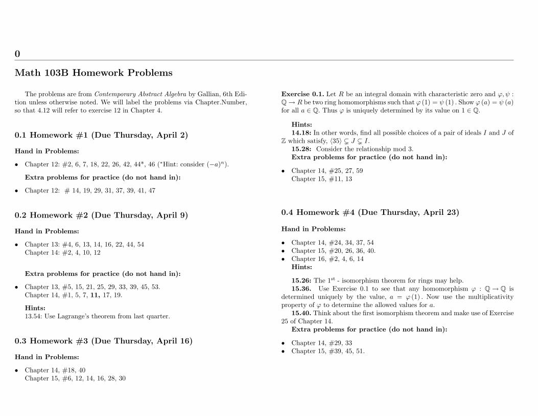
Math 103B Homework Problems

The problems are from Contemporary Abstract Algebra by Gallian, 6th Edi-tion unless otherwise noted. We will label the problems via Chapter.Number,so that 4.12 will refer to exercise 12 in Chapter 4.

0.1 Homework #1 (Due Thursday, April 2)

Hand in Problems:

• Chapter 12: #2, 6, 7, 18, 22, 26, 42, 44*, 46 (∗Hint: consider (−a)n).

Extra problems for practice (do not hand in):

• Chapter 12: # 14, 19, 29, 31, 37, 39, 41, 47


Hand in Problems:

• Chapter 13: #4, 6, 13, 14, 16, 22, 44, 54Chapter 14: #2, 4, 10, 12


• Chapter 13, #5, 15, 21, 25, 29, 33, 39, 45, 53.Chapter 14, #1, 5, 7, 11, 17, 19.

Hints:13.54: Use Lagrange’s theorem from last quarter.


Hand in Problems:

• Chapter 14, #18, 40Chapter 15, #6, 12, 14, 16, 28, 30

Exercise 0.1. Let R be an integral domain with characteristic zero and ϕ,ψ :Q→ R be two ring homomorphisms such that ϕ (1) = ψ (1) . Show ϕ (a) = ψ (a)for all a ∈ Q. Thus ϕ is uniquely determined by its value on 1 ∈ Q.

Hints:14.18: In other words, find all possible choices of a pair of ideals I and J of

Z which satisfy, 〈35〉 ( J ( I.15.28: Consider the relationship mod 3.Extra problems for practice (do not hand in):

• Chapter 14, #25, 27, 59Chapter 15, #11, 13


Hand in Problems:

• Chapter 14, #24, 34, 37, 54• Chapter 15, #20, 26, 36, 40.• Chapter 16, #2, 4, 6, 14

Hints:

15.26: The 1st - isomorphism theorem for rings may help.15.36. Use Exercise 0.1 to see that any homomorphism ϕ : Q→ Q is

determined uniquely by the value, a = ϕ (1) . Now use the multiplicativityproperty of ϕ to determine the allowed values for a.

15.40. Think about the first isomorphism theorem and make use of Exercise25 of Chapter 14.


• Chapter 14, #29, 33• Chapter 15, #39, 45, 51.

4 0 Math 103B Homework Problems


Hand in Problems:

Exercise 0.2 (This problem is to be handed in!). Let R be a commutativering with identity. Then R is a field iff R has no non-trivial proper ideals. (Recallthat I ⊂ R is the trivial ideal if I = {0} and is a proper ideal if I R.)

• Chapter 14, #28, 32, 36, 52• Chapter 15, #58, 60

Hints:14.36: Let S := {a+ bi : a ∈ Z4 and b ∈ Z2} . To count the number of ele-

ment in Z [i] / 〈2 + 2i〉 you might show

S 3 (a+ bi)ψ−→ [a+ bi] ∈ Z [i] / 〈2 + 2i〉

is a bijection.14.52: One way is to prove that Z [i] / 〈1− i〉 is isomorphic to Z2.Extra problems for practice (do not hand in):

• Chapter 14, #31• Chapter 15, #27, 29, 42, 62

0.6 Homework #6 (Due Thursday, May 7)

Hand in Problems:

• Chapter 16, #12, 18, 20, 24, 30, 36, 38, 48.Hint:

16.20. Think about the roots of the polynomial h = f − g.Extra problems for practice (do not hand in):

• Chapter 16, #1, 11, 13, 15, 19, 41


Hand in Problems:

• Chapter 17, #2, 4, 6, 8, 12, 14, 25 (17.4 is a special case of 17.25!)


• Chapter 17, #1, 3, 5, 7, 21


Hand in all problems below:

• Chapter 17, #10a, c, e, l0 b & d, 32

Exercise 0.3. Prove Proposition 20.4.

Exercise 0.4. Let ψ : R→ T be an onto ring homomorphism of commutativerings, R and T and I := ker (ψ) .

1. Explain why ψ : R [x]→ T [x] is onto.2. Show ker

(ψ)

= I [x] .3. Use the first isomorphism theorem to conclude R [x] /I [x] is isomorphicT [x] .

Exercise 0.5. Let R be a commutative ring and I ⊂ R be an ideal. Use theresults of Exercise 0.4 to show R [x] /I [x] is isomorphic to (R/I) [x] .

Exercise 0.6. Use Exercise 0.5 to give another proof Exercise 16.38 on page300 of the book. This proof should be very short and similar in spirit to theproof of Gauss’ Lemma on p. 305 of the book.

Exercise 0.7. Prove Proposition 18.7.

Exercise 0.8. Prove Proposition 23.3

Exercise 0.9. Show x8 − 20/9 ∈ Q [x] is irreducible over Q. Conclude that8√

20/9 /∈ Q.

Hints:17.10b & d. Try the mod p irreducibility test, using some small prime p.

Follow the method of examples 7 and 8 in the book.17.32. One possibility is to show Z [x] /

⟨x2 + 1

⟩is isomorphic to a ring we

have studied frequently. Then use Theorems 14.3 and 14.4 of the book.


Part II

Math 103B Lecture Notes

1

Lecture 1

1.1 Definition of Rings and Examples

A ring will be a set of elements, R, with both an addition and multiplicationoperation satisfying a number of “natural” axioms.

Axiom 1.1 (Axioms for a ring) Let R be a set with 2 binary operationscalled addition (written a + b) and multiplication (written ab). R is called aring if for all a, b, c ∈ R we have

1. (a+ b) + c = a+ (b+ c)2. There exists an element 0 ∈ R which is an identity for +.3. There exists an element −a ∈ R such that a+ (−a) = 0.4. a+ b = b+ a.5. (ab)c = a(bc).6. a(b+ c) = ab+ ac and (b+ c)a = ba+ bc.

Items 1. – 4. are the axioms for an abelian group, (R,+) . Item 5. says mul-tiplication is associative, and item 6. says that is both left and right distributiveover addition. Thus we could have stated the definition of a ring more succinctlyas follows.

Definition 1.2. A ring R is a set with two binary operations “+” = additionand “·”= multiplication, such that (R,+) is an abelian group (with identityelement we call 0), “·” is an associative multiplication on R which is both leftand right distributive over addition.

Remark 1.3. The multiplication operation might not be commutative, i.e., ab 6=ba for some a, b ∈ R. If we have ab = ba for all a, b ∈ R, we say R is acommutative ring. Otherwise R is noncommutative.

Definition 1.4. If there exists and element 1 ∈ R such that a1 = 1a = a for alla ∈ R, then we call 1 the identity element of R [the book calls it the unity.]

Most of the rings that we study in this course will have an identity element.

Lemma 1.5. If R has an identity element 1, then 1 is unique. If an elementa ∈ R has a multiplicative inverse b, then b is unique, and we write b = a−1.

Proof. Use the same proof that we used for groups! I.e. 1 = 1 · 1′ = 1′ andif b, b′ are both inverses to a, then b = b (ab′) = (ba) b′ = b′.

Notation 1.6 (Subtraction) In any ring R, for a ∈ R we write the additiveinverse of a as (−a). So at a + (−a) = (−a) + a = 0 by definition. For anya, b ∈ R we abbreviate a+ (−b) as a− b.

Let us now give a number of examples of rings.

Example 1.7. Here are some examples of commutative rings that we are alreadyfamiliar with.

1. Z= all integers with usual + and ·.2. Q= all mn such that m,n ∈ Z with n 6= 0, usual + and ·. (We will generalize

this later when we talk about “fields of fractions.”)3. R= reals, usual + and ·.4. C= all complex numbers, i.e. {a+ ib : a, b ∈ R} , usual + and · operations.

(We will explicitly verify this in Proposition 3.7 below.)

Example 1.8. 2Z = {. . . ,−4,−2, 0, 2, 4, . . . } is a ring without identity.

Example 1.9 (Integers modulo m). For m ≥ 2, Zm = {0, 1, 2, . . . ,m− 1} with

+ = addition modm· = multiplication modn.

Recall from last quarter that (Zm,+) is an abelian group and we showed,

[(ab) modm · c] modm = [abc] = [a (bc) modm] modm (associativity)

and

[a · (b+ c) modm] modm = [a · (b+ c)] modm= [ab+ ac] modm = (ab) modm+ (ac) modm

which is the distributive property of multiplication modm. Thus Zm is a ringwith identity, 1.

8 1 Lecture 1

Example 1.10. M2(F ) = 2 × 2 matrices with entries from F , where F = Z, Q,R, or C with binary operations;[

a bc d

]+[a′ b′

c′ d′

]=[a+ a′ b+ b′

c+ c′ d+ d′

](addition)

[a bc d

] [a′ b′

c′ d′

]=[aa′ + bc′ ab′ + bd′

ca′ + dc′ cb′ + dd′

]. (multiplication)

That is multiplication is the usual matrix product. You should have checked inyour linear algebra course that M2 (F ) is a non-commutative ring with identity,

I =[

1 00 1

].

For example let us check that left distributive law in M2(Z);[a bc d

]([e fg h

]+[p qr s

])=[a bc d

] [p+ e f + qg + r h+ s

]=[b (g + r) + a (p+ e) a (f + q) + b (h+ s)d (g + r) + c (p+ e) c (f + q) + d (h+ s)

]=[bg + ap+ br + ae af + bh+ aq + bsdg + cp+ dr + ce cf + dh+ cq + ds

]while [

a bc d

] [e fg h

]+[a bc d

] [p qr s

]=[bg + ae af + bhdg + ce cf + dh

]+[ap+ br aq + bscp+ dr cq + ds

]=[bg + ap+ br + ae af + bh+ aq + bsdg + cp+ dr + ce cf + dh+ cq + ds

]which is the same result as the previous equation.

Example 1.11. We may realize C as a sub-ring of M2 (R) as follows. Let

I =[

1 00 1

]∈M2 (R) and i :=

[0 −11 0

]and then identify z = a+ ib with

aI+bi := a

[1 00 1

]+ b

[0 −11 0

]=[a −bb a

].

Since

i2 =[

0 −11 0

] [0 −11 0

]= I

it is straight forward to check that

(aI+bi) (cI+di) = (ac− bd) I + (bc+ ad) i and(aI+bi) + (cI+di) = (a+ c) I + (b+ d) i

which are the standard rules of complex arithmetic. The fact that C is a ringnow easily follows from the fact that M2 (R) is a ring.

In this last example, the reader may wonder how did we come up with the

matrix i :=[

0 −11 0

]to represent i. The answer is as follows. If we view C as R2

in disguise, then multiplication by i on C becomes,

(a, b) ∼ a+ ib→ i (a+ ib) = −b+ ai ∼ (−b, a)

while

i(ab

)=[

0 −11 0

](ab

)=(−ba

).

Thus i is the 2× 2 real matrix which implements multiplication by i on C.

Theorem 1.12 (Matrix Rings). Suppose that R is a ring and n ∈ Z+. LetMn (R) denote the n× n – matrices A = (Aij)

ni,j=1 with entries from R. Then

Mn (R) is a ring using the addition and multiplication operations given by,

(A+B)ij = Aij +Bij and

(AB)ij =∑k

AikBkj .

Moreover if 1 ∈ R, then

I :=

1 0 0

0. . . 0

0 0 1

is the identity of Mn (R) .

Proof. I will only check associativity and left distributivity of multiplicationhere. The rest of the proof is similar if not easier. In doing this we will makeuse of the results about sums in the Appendix 1.2 at the end of this lecture.

Let A, B, and C be n× n – matrices with entries from R. Then


1.2 Appendix: Facts about finite sums 9

[A (BC)]ij =∑k

Aik (BC)kj =∑k

Aik

(∑l

BklClj

)=∑k,l

AikBklClj

while

[(AB)C]ij =∑l

(AB)il Clj =∑l

(∑k

AikBkl

)Clj

=∑k,l

AikBklClj .

Similarly,

[A (B + C)]ij =∑k

Aik (Bkj + Ckj) =∑k

(AikBkj +AikCkj)

=∑k

AikBkj +∑k

AikCkj = [AB]ij + [AC]ij .

Example 1.13. In Z6, 1 is an identity for multiplication, but 2 has no multi-plicative inverse. While in M2(R), a matrix A has a multiplicative inverse ifand only if det(A) 6= 0.

Example 1.14 (Another ring without identity). Let

R ={[

0 a0 0

]: a ∈ R

}with the usual addition and multiplication of matrices.[

0 a0 0

] [0 b0 0

]=[0 00 0

].

The identity element for multiplication “wants” to be[1 00 1

], but this is not in

R.More generally if (R,+) is any abelian group, we may make it into a ring

in a trivial way by setting ab = 0 for all a, b ∈ R. This ring clearly has nomultiplicative identity unless R = {0} is the trivial group.

1.2 Appendix: Facts about finite sums

Throughout this section, suppose that (R,+) is an abelian group, Λ is any set,and Λ 3 λ→ rλ ∈ R is a given function.

Theorem 1.15. Let F := {A ⊂ Λ : |A| <∞} . Then there is a unique function,S : F → R such that;

1. S (∅) = 0,2. S ({λ}) = rλ for all λ ∈ Λ.3. S (A ∪B) = S (A) + S (B) for all A,B ∈ F with A ∩B = ∅.

Moreover, for any A ∈ F , S (A) only depends on {rλ}λ∈A .

Proof. Suppose that n ≥ 2 and that S (A) has been defined for all A ∈ Fwith |A| < n in such a way that S satisfies items 1. – 3. provided that |A ∪B| <n. Then if |A| = n and λ ∈ A, we must define,

S (A) = S (A \ {λ}) + S ({λ}) = S (A \ {λ}) + rλ.

We should verify that this definition is independent of the choice of λ ∈ A. Tosee this is the case, suppose that λ′ ∈ A with λ′ 6= λ, then by the inductionhypothesis we know,

S (A \ {λ}) = S ([A \ {λ, λ′}] ∪ {λ′})= S (A \ {λ, λ′}) + S ({λ′}) = S (A \ {λ, λ′}) + rλ′

so that

S (A \ {λ}) + rλ = [S (A \ {λ, λ′}) + rλ′ ] + rλ

= S (A \ {λ, λ′}) + (rλ′ + rλ)= S (A \ {λ, λ′}) + (rλ + rλ′)= [S (A \ {λ, λ′}) + rλ] + rλ′

= [S (A \ {λ, λ′}) + S ({λ})] + rλ′

= S (A \ {λ′}) + rλ′

as desired. Notice that the “moreover” statement follows inductively using thisdefinition.

Now suppose that A,B ∈ F with A∩B = ∅ and |A ∪B| = n. Without lossof generality we may assume that neither A or B is empty. Then for any λ ∈ B,we have using the inductive hypothesis, that

S (A ∪B) = S (A ∪ [B \ {λ}]) + rλ = (S (A) + S (B \ {λ})) + rλ

= S (A) + (S (B \ {λ}) + rλ) = S (A) + (S (B \ {λ}) + S ({λ}))= S (A) + S (B) .


10 1 Lecture 1

Thus we have defined S inductively on the size of A ∈ F and we had nochoice in how to define S showing S is unique.

Notation 1.16 Keeping the notation used in Theorem 1.15, we will denoteS (A) by

∑λ∈A rλ. If A = {1, 2, . . . , n} we will often write,

∑λ∈A

rλ =n∑i=1

ri.

Corollary 1.17. Suppose that A = A1 ∪ · · · ∪ An with Ai ∩ Aj = ∅ for i 6= jand |A| <∞. Then

S (A) =n∑i=1

S (Ai) i.e.∑λ∈A

rλ =n∑i=1

(∑λ∈Ai

rλ

).

Proof. As usual the proof goes by induction on n. For n = 2, the assertionis one of the defining properties of S (A) :=

∑λ∈A rλ. For n ≥ 2, we have using

the induction hypothesis and the definition of∑ni=1 S (Ai) that

S (A1 ∪ · · · ∪An) = S (A1 ∪ · · · ∪An−1) + S (An)

=n−1∑i=1

S (Ai) + S (An) =n∑i=1

S (Ai) .

Corollary 1.18 (Order does not matter). Suppose that A is a finite subsetof Λ and B is another set such that |B| = n = |A| and σ : B → A is a bijectivefunction. Then ∑

b∈B

rσ(b) =∑a∈A

ra.

In particular if σ : A→ A is a bijection, then∑a∈A

rσ(a) =∑a∈A

ra.

Proof. We again check this by induction on n = |A| . If n = 1, then B = {b}and A = {a := σ (b)} , so that∑

x∈Brσ(x) = rσ(b) =

∑a∈A

ra

as desired. Now suppose that N ≥ 1 and the corollary holds whenever n ≤ N.If |B| = N + 1 = |A| and σ : B → A is a bijective function, then for any b ∈ B,we have with B′ := B′ \ {b} that

∑x∈B

rσ(x) =∑x∈B′

rσ(x) + rσ(b).

Since σ|B′ : B′ → A′ := A \ {σ (b)} is a bijection, it follows by the inductionhypothesis that

∑x∈B′ rσ(x) =

∑λ∈A′ rλ and therefore,∑

x∈Brσ(x) =

∑λ∈A′

rλ + rσ(b) =∑λ∈A

rλ.

Lemma 1.19. If {aλ}λ∈Λ and {bλ}λ∈Λ are two sequences in R, then∑λ∈A

(aλ + bλ) =∑λ∈A

aλ +∑λ∈A

bλ.

Moreover, if we further assume that R is a ring, then for all r ∈ R we have theright and left distributive laws;,

r ·∑λ∈A

aλ =∑λ∈A

r · aλ and(∑λ∈A

aλ

)· r =

∑λ∈A

aλ · r.

Proof. This follows by induction. Here is the key step. Suppose that α ∈ Aand A′ := A \ {α} , then∑

λ∈A

(aλ + bλ) =∑λ∈A′

(aλ + bλ) + (aα + bα)

=∑λ∈A′

aλ +∑λ∈A′

bλ + (aα + bα) (by induction)

=

(∑λ∈A′

aλ + aλ+

)(∑λ∈A′

bλ + bα

) (commutativity

and associativity

)=∑λ∈A

aλ +∑λ∈A

bλ.

The multiplicative assertions follows by induction as well,

r ·∑λ∈A

aλ = r ·

(∑λ∈A′

aλ + aα

)= r ·

(∑λ∈A′

aλ

)+ r · aα

=

(∑λ∈A′

r · aλ

)+ r · aα

=∑λ∈A

r · aλ.


2

Lecture 2

Recall that a ring is a set, R, with two binary operations “+” = additionand “·”= multiplication, such that (R,+) is an abelian group (with identityelement we call 0), (·) is an associative multiplication on R which is left and rightdistributive over “+.” Also recall that if there is a multiplicative identity, 1 ∈ R(so 1a = a1 = a for all a), we say R is a ring with identity (unity). Furthermorewe write a − b for a + (−b) . This shows the importance of distributivity. Wenow continue with giving more examples of rings.

Example 2.1. Let R denote the continuous functions, f : R→ R such thatlimx→±∞ f (x) = 0. As usual, let f + g and f · g be pointwise addition andmultiplication of functions, i.e.

(f + g) (x) = f (x) + g (x) and (f · g) (x) = f (x) g (x) for all x ∈ R.

Then R is a ring without identity. (If we remove the restrictions on the functionsat infinity, R would be a ring with identity, namely 1 (x) ≡ 1.)

Example 2.2. For any collection of rings R1, R2, . . . , Rm, define the direct sumto be

R = R1 ⊕ · · · ⊕Rn = {(r1, r2, . . . , rn) : ri ∈ Ri all i}

the set of all m-tuples where the ith coordinate comes from Ri. R is a ring ifwe define

(r1, r2, . . . , rm) + (s1, s2, . . . , sm) = (r1s1, r2s2, . . . , rmsm),

and

(r1, r2, . . . , rm) + (s1, s2, . . . , sm) = (r1 + s1, r2 + s2, . . . , rm + sm).

The identity element 0 is (0, 0, . . . , 0). (Easy to check)

2.1 Polynomial Ring Examples

Example 2.3 (Polynomial rings). Let R = Z, Q, R, or Z and let R [x] denote thepolynomials in x with coefficients from R. We add and multiply polynomials inthe usual way. For example if f = 3x2 − 2x+ 5 and g = 5x2 + 1, then

f + g = 8x2 − 2x+ 6 and

fg = (5x3 + 1)(3x2 − 2x+ 5)

= 5− 2x+ 3x2 + 25x3 − 10x4 + 15x5.

One may check (see Theorem 2.4 below) that R [x] with these operations is acommutative ring with identity, 1 = 1.These rules have been chosen so that(f + g) (α) = f (α) + g (α) and (f · g) (α) = f (α) g (α) for all α ∈ R where

f (α) :=∞∑i=0

aiαi.

Theorem 2.4. Let R be a ring and R [x] denote the collection of polynomialswith the usual addition and multiplication rules of polynomials. Then R [x] isagain a ring. To be more precise,

R [x] =

{p =

∞∑i=0

pixi : pi ∈ R with pi = 0 a.a.

},

where we say that pi = 0 a.a. (read as almost always) provided that|{i : pi 6= 0}| <∞. If q :=

∑∞i=0 qix

i ∈ R [x] , then we set,

p+ q :=∞∑i=0

(pi + qi)xi and (2.1)

p · q :=∞∑i=0

( ∑k+l=i

pkql

)xi =

∞∑i=0

(i∑

k=0

pkqi−k

)xi. (2.2)

Proof. The proof is similar to the matrix group examples. Let me only saya few words about the associativity property of multiplication here, since thisis the most complicated property to check. Suppose that r =

∑∞i=0 rix

i, then

12 2 Lecture 2

p (qr) =∞∑n=0

∑i+j=n

pi (qr)j

xn

=∞∑n=0

∑i+j=n

pi

∑k+l=j

qkrl

xn

=∞∑n=0

( ∑i+k+l=n

piqkrl

)xn.

As similar computation shows,

(pq) r =∞∑n=0

( ∑i+k+l=n

piqkrl

)xn

and hence the multiplication rule in Eq. (2.2) is associative.

2.2 Subrings and Ideals I

We now define the concept of a subring in a way similar to the concept ofsubgroup.

Definition 2.5 (Subring). Let R be a ring. If S is subset of R which is itselfa ring under the same operations +, · of R restricted to the set S, then S iscalled a subring of R.

Lemma 2.6 (Subring test). S ⊂ R is a subring if and only if S is a subgroupof (R,+) and S is closed under multiplication. In more detail, S is a subringof R, iff for all a, b ∈ S, that

a+ b ∈ S, − a ∈ S, and ab ∈ S.

Alternatively we may check that

a− b ∈ S, and ab ∈ S for all a, b ∈ S.

Put one last way, S is a subring of R if (S,+) is a subgroup of (R,+) which isclosed under the multiplication operation, i.e. S · S ⊂ S.

Proof. Either of the conditions, a + b ∈ S, −a ∈ S or a − b ∈ S for alla, b ∈ S implies that (S,+) is a subgroup of (R,+) . The condition that (S, ·)is a closed shows that “·” is well defined on S. This multiplication on S theninherits the associativity and distributivity laws from those on R.

Definition 2.7 (Ideals). Let R be a ring. A (two sided) ideal, I, of R is asubring, I ⊂ R such that RI ⊂ R and IR ⊂ R. Alternatively put, I ⊂ R is anideal if (I,+) is a subgroup of (R,+) such that RI ⊂ R and IR ⊂ R. (Noticethat every ideal, I, of R is also a subring of R.)

Example 2.8. Suppose that R is a ring with identity 1 and I is an ideal. If 1 ∈ I,then I = R since R = R · 1 ⊂ RI ⊂ I.

Example 2.9. Given a ring R, R itself and {0} are always ideals of R. {0} is thetrivial ideal. An ideal (subring) I ⊂ R for which I 6= R is called a proper ideal(subring).

Example 2.10. If R is a commutative ring and b ∈ R is any element, then theprinciple ideal generated by b, denoted by 〈b〉 or Rb, is

I = Rb = {rb : r ∈ R}.

To see that I is an ideal observer that if r, s ∈ R, then rb and sb are genericelements of I and

rb− sb = (r − s)b ∈ Rb.

Therefore I is an additive subgroup of R. Moreover, (rb) s = s (rb) = (sr) b ∈ Iso that RI = IR ⊂ I.

Theorem 2.11. Suppose that R = Z or R = Zm for some m ∈ Z+. Then thesubgroups of (R,+) are the same as the subrings of R which are the same asthe ideals of R. Moreover, every ideal of R is a principle ideal.

Proof. If R = Z, then 〈m〉 = mZ inside of Z is the principle ideal generatedby m. Since every subring, S ⊂ Z is also a subgroup and all subgroups of Z areof the form mZ for some m ∈ Z, it flows that all subgroups of (Z,+) are in factalso principle ideals.

Suppose now that R = Zn. Then again for any m ∈ Zn,

〈m〉 = {km : k ∈ Z} = mZn (2.3)

is the principle ideal in Zn generated by m. Conversely if S ⊂ Zn is a sub-ring,then S is in particular a subgroup of Zn. From last quarter we know that thisimplies S = 〈m〉 = 〈gcd (n,m)〉 for some m ∈ Zn. Thus every subgroup of(Zn,+) is a principle ideal as in Eq. (2.3).

Example 2.12. The set,

S ={[a b0 d

]: a, b, d ∈ R

},

is a subring of M2(R). To check this observe that;


2.2 Subrings and Ideals I 13[a b0 d

]−[a′ b′

0 d′

]=[a− a b− b′

0 d− d′]∈ S

and [a b0 d

] [a′ b′

0 d′

]=[a′a ab′ + bd′

0 dd′

]∈ S.

S is not an ideal since,[0 01 0

] [a b0 d

]=[0 0a b

]/∈ S if a 6= 0.

Example 2.13. Consider Zm and the subset U(m) the set of units in Zm. ThenU(m) is never a subring of Zm, because 0 /∈ U(m).

Example 2.14. The collection of matrices,

S ={[

0 ab c

]: a, b, c ∈ R

},

is not a subring of M2(R). It is an additive subgroup which is however notclosed under matrix multiplication;[

0 ab c

] [0 a′

b′ c′

]=[ab′ ac′

cb′ ba+ cc′

]/∈ S

Definition 2.15. Let R be a ring with identity. We say that S ⊂ R is a unitalsubring of R if S is a sub-ring containing 1R. (Most of the subrings we willconsider later will be unital.)

Example 2.16. Here are some examples of unital sub-rings.

1. S in Example 2.12 is a unital sub-ring of M2 (R) .2. The polynomial functions on R is a unital sub-ring of the continuous func-

tions on R.3. Z [x] is a unital sub-ring of Q [x] or R [x] or C [x] .4. Z [i] := {a+ ib : a, b ∈ Z} is a unital subring of C.

Example 2.17. Here are a few examples of non-unital sub-rings.

1. nZ ⊂ Z is a non-unital subring of Z for all n 6= 0 since nZ does not evencontain an identity element.

2. If R = Z8, then every non-trivial proper subring, S = 〈m〉 , of R has noidentity. The point is if k ∈ Z8 is going to be an identity for some sub-ringof Z8, then k2 = k. It is now simple to check that k2 = k in Z8 iff k = 0or 1 which are not contained in any proper non-trivial sub-ring of Z8. (SeeRemark 2.18 below.)

3. Let R := Z6 and S = 〈2〉 = {0, 2, 4} is a sub-ring of Z6. Moreover, one seesthat 1S = 4 is the unit in S (42 = 4 and 4 · 2 = 2) which is not 1R = 1.Thus again, S is not a unital sub-ring of Z6.

4. The set,

S ={[a 00 0

]: a ∈ R

}⊂ R = M2(R),

is a subring of M2 (R) with

1S =[1 00 0

]6=[1 00 1

]= 1R

and hence is not a unital subring of M2 (R) .5. Let v be a non-zero column vector in R2 and define,

S := {A ∈M2 (R) : Av = 0} .

Then S is a non-unital subring of M2 (R) which is not an ideal. (You shouldverify these assertions yourself!)

Remark 2.18. Let n ∈ Z+ and S := 〈m〉 be a sub-ring of Zn. It is natural toask, when does S have an identity element. To answer this question, we beginby looking for m ∈ Zn such that m2 = m. Given such a m, we claim that m isan identity for 〈m〉 since

(km)m = km2 = k1m for all km ∈ 〈m〉 .

The condition that m2 = m is equivalent to m (m− 1) = 0, i.e. n|m (m− 1) .Thus 〈m〉 = 〈gcd (n,m)〉 is a ring with identity iff n|m (m− 1) .

Example 2.19. Let us take m = 6 in the above remark so that m (m− 1) =30 = 3 · 2 · 5. In this case 10, 15 and 30 all divide m (m− 1) and therefore 6is the identity element in 〈6〉 thought of as a subring of either, Z10, or Z15, orZ30. More explicitly 6 is the identity in

〈6〉 = 〈gcd (6, 10)〉 = 〈2〉 = {0, 2, 4, 6, 8} ⊂ Z10,

〈6〉 = 〈gcd (6, 15)〉 = 〈3〉 = {0, 3, 6, 9, 12} ⊂ Z15, and〈6〉 = 〈gcd (6, 30)〉 = {0, 6, 12, 18, 24} ⊂ Z30.

Example 2.20. On the other hand there is no proper non-trivial subring of Z8

which contains an identity element. Indeed, if m ∈ Z8 and 8 = 23|m (m− 1) ,then either 23|m if m is even or 23| (m− 1) if m is odd. In either the onlym ∈ Z8 with this property is m = 0 and m = 1. In the first case 〈0〉 = {0} isthe trivial subring of Z8 and in the second case 〈1〉 = Z8 is not proper.


3

Lecture 3

3.1 Some simple ring facts

The next lemma shows that the distributive laws force 0, 1, and the symbol“−” to behave in familiar ways.

Lemma 3.1 (Some basic properties of rings). Let R be a ring. Then;

1. a0 = 0 = 0a for all a ∈ R.2. (−a)b = − (ab) = a(−b) for all a, b ∈ R3. (−a)(−b) = ab for all a, b ∈ R. In particular, if R has identity 1, then

(−1)(−1) = 1 and(−1)a = −a for all a ∈ R.

(This explains why minus times minus is a plus! It has to be true in anystructure with additive inverses and distributivity.)

4. If a, b, c ∈ R, then a (b− c) = ab− ac and (b− c) a = ba− ca.

Proof. For all a, b ∈ R;

1. a0 + 0 = a0 = a(0 + 0) = a0 + a0, and hence by cancellation in the abeliangroup, (R,+) , we conclude that , so 0 = a0. Similarly one shows 0 = 0a.

2. (−a)b+ab = (−a+a)b = 0b = 0, so (−a)b = − (ab). Similarly a(−b) = −ab.3. (−a)(−b) = − (a(−b)) = −(−(ab)) = ab, where in the last equality we have

used the inverting an element in a group twice gives the element back.4. This last item is simple since,

a (b− c) := a (b+ (−c)) = ab+ a (−c) = ab+ (−ac) = ab− ac.

Similarly one shows that (b− c) a = ba− ca.

In proofs above the reader should not be fooled into thinking these thingsare obvious. The elements involved are not necessarily familiar things like realnumbers. For example, in M2(R) item 2 states, (−I)A = −(IA) = −A, i.e.[

−1 00 −1

] [a bc d

]=[−a −b−c −d

]X

The following example should help to illustrate the significance of Lemma 3.1.

Example 3.2. Consider R = 〈2〉 = {0, 2, 4, 6, 8} ⊂ Z10. From Example 2.19 weknow that 1R = 6 which you can check directly as well. So −1R = −6 mod 10 =4. Taking a = 2 let us write out the meaning of the identity, (−1R) · a = −a;

(−1R) · a = 4 · 2 = 8 = −a.

Let us also work out (−2) (−4) and compare this with 2 · 4 = 8;

(−2) (−4) = 8 · 6 = 48 mod 10 = 8.

Lastly consider,

4 · (8− 2) = 4 · 6 = 24 mod 10 = 4 while4 · 8− 4 · 2 = 2− 8 = −6 mod 10 = 4.

3.2 The R [S] subrings I

Here we will construct some more examples of rings which are closely relatedto polynomial rings. In these examples, we will be given a commutative ring R(usually commutative) and a set S equipped with some sort of multiplication,we then are going to define R [S] to be the collection of linear combinations ofelements from the set, ∪∞n=0RS

n. Here RSn consists of formal symbols of theform rs1 . . . sn with r ∈ R and si ∈ S. The next proposition gives a typicalexample of what we have in mind.

A typical case will be where S = {s1, . . . , sn} is a finite set then

Proposition 3.3. If R ⊂ R is a sub-ring of a commutative ring R and S ={s1, . . . , sn} ⊂ R. Let

R [S] = R [s1, . . . , sn] =

{∑k

aksk : ak ∈ R with ak = 0 a.a.

},

where k = (k1, . . . kn) ∈ Nn and sk = sk11 . . . sknn with a0s

0 := a0 ∈ R. ThenR [s1, . . . , sn] is a sub-ring of R.

16 3 Lecture 3

Proof. If f =∑k aks

k and g =∑k bks

k, then

f + g =∑k

(ak + bk) sk ∈ R [S] ,

−g =∑k

−bksk ∈ R [S] , and

f · g =∑k

aksk ·∑l

blsl

=∑k,l

akblsksl =

∑k,l

akblsk+l

=∑n

( ∑k+l=n

akbl

)sn ∈ R [S] .

Example 3.4 (Gaussian Integers). Let i :=√−1 ∈ C. Then Z [i] =

{x+ yi : x, y ∈ Z} . To see this notice that i2 = −1 ∈ Z, and therefore

∞∑k=0

ak (i)k =∞∑l=0

[a4l (i)

4l + a4l+1 (i)4l+1 + a4l+2 (i)4l+2 + a4l+3 (i)4l+3]

=∞∑l=0

[a4l + a4l+1i− a4l+2 − a4l+3i]

=∞∑l=0

[a4l − a4l+2] +

( ∞∑l=0

[a4l+1 − a4l+3]

)i

= x+ yi

where

x =∞∑l=0

[a4l − a4l+2] and y =∞∑l=0

[a4l+1 − a4l+3] .

Example 3.5. Working as in the last example we see that

Z[√

2]

={a+ b

√2 : a, b ∈ Z

}is a sub-ring of R.

Example 3.6 (Gaussian Integers mod m). For any m ≥ 2, let

Zm [i] = {x+ yi : x, y ∈ Zm}

with the obvious addition rule and multiplication given by

(x+ yi) (u+ vi) = ux− vy + (uy + vx) i in Zm.

The next proposition shows that this is a commutative ring with identity, 1.

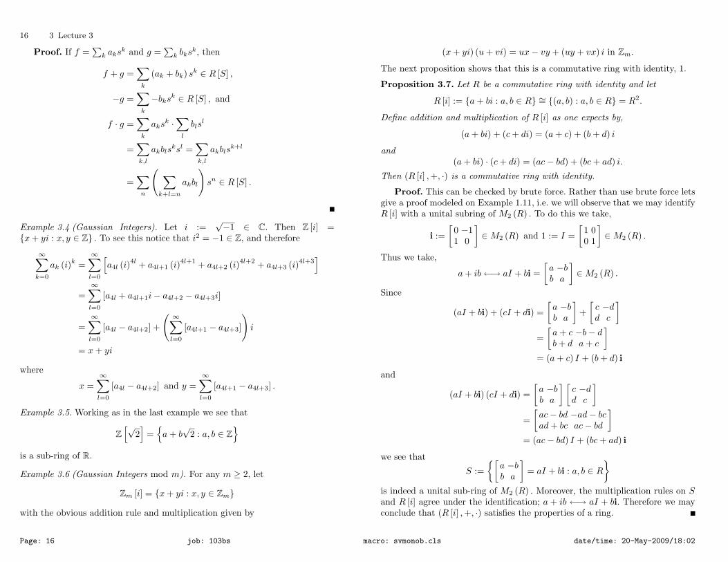
Proposition 3.7. Let R be a commutative ring with identity and let

R [i] := {a+ bi : a, b ∈ R} ∼= {(a, b) : a, b ∈ R} = R2.

Define addition and multiplication of R [i] as one expects by,

(a+ bi) + (c+ di) = (a+ c) + (b+ d) i

and(a+ bi) · (c+ di) = (ac− bd) + (bc+ ad) i.

Then (R [i] ,+, ·) is a commutative ring with identity.

Proof. This can be checked by brute force. Rather than use brute force letsgive a proof modeled on Example 1.11, i.e. we will observe that we may identifyR [i] with a unital subring of M2 (R) . To do this we take,

i :=[

0 −11 0

]∈M2 (R) and 1 := I =

[1 00 1

]∈M2 (R) .

Thus we take,

a+ ib←→ aI + bi =[a −bb a

]∈M2 (R) .

Since

(aI + bi) + (cI + di) =[a −bb a

]+[c −dd c

]=[a+ c −b− db+ d a+ c

]= (a+ c) I + (b+ d) i

and

(aI + bi) (cI + di) =[a −bb a

] [c −dd c

]=[ac− bd −ad− bcad+ bc ac− bd

]= (ac− bd) I + (bc+ ad) i

we see that

S :={[

a −bb a

]= aI + bi : a, b ∈ R

}is indeed a unital sub-ring of M2 (R) . Moreover, the multiplication rules on Sand R [i] agree under the identification; a + ib ←→ aI + bi. Therefore we mayconclude that (R [i] ,+, ·) satisfies the properties of a ring.


3.3 Appendix: R [S] rings II 17

3.3 Appendix: R [S] rings II

You may skip this section on first reading.Definition 3.8. Suppose that S is a set which is equipped with an associativebinary operation, ·, which has a unique unit denoted by e. (We do not assumethat (S, ·) has inverses. Also suppose that R is a ring, then we let R [S] consistof the formal sums,

∑s∈S ass where {as}s∈S ⊂ R is a sequence with finite

support, i.e. |{s ∈ S : as 6= 0}| <∞. We define two binary operations on R [S]by, ∑

s∈Sass+

∑s∈S

bss :=∑s∈S

(as + bs) s

and ∑s∈S

ass ·∑s∈S

bss =∑s∈S

ass ·∑t∈S

btt

=∑s,t∈S

asbtst =∑u∈S

(∑st=u

asbt

)u.

So really we R [S] are those sequences a := {as}s∈S with finite support with theoperations,

(a+ b)s = as + bs and (a · b)s =∑uv=s

aubv for all s ∈ S.

Theorem 3.9. The set R [S] equipped with the two binary operations (+, ·) isa ring.

Proof. Because (R,+) is an abelian group it is easy to check that (R [S] ,+)is an abelian group as well. Let us now check that · is associative on R [S] . Tothis end, let a, b, c ∈ R [S] , then

[a (bc)]s =∑uv=s

au (bc)v =∑uv=s

au

∑αβ=v

bαcβ

=∑uαβ=s

aubαcβ

while

[(ab) c]s =∑αβ=s

(ab)α cβ =∑αβ=s

∑uv=α

aubvcβ

=∑uvβ=s

aubvcβ =∑uαβ=s

aubαcβ = [a (bc)]s

as desired. Secondly,

[a · (b+ c)]s =∑uv=s

au (b+ c)v =∑uv=s

au (bv + cv)

=∑uv=s

aubv +∑uv=s

aucv

= [a · b]s + [a · c]s = [a · b+ a · c]s

from which it follows that a · (b+ c) = a · b + a · c. Similarly one shows that(b+ c) · a = b · a+ c · a.

Lastly if S has an identity, e, and es := 1s=e ∈ R, then

[a · e]s =∑uv=s

auev = as

from which it follows that e is the identity in R [S] .

Example 3.10 (Polynomial rings). Let x be a formal symbol and let S :={xk : k = 0, 1, 2 . . .

}with xkxl := xk+l being the binary operation of S. No-

tice that x0 is the identity in S under this multiplication rule. Then for anyring R, we have

R [S] =

{p (x) :=

n∑k=0

pkxk : pk ∈ R and n ∈ N

}.

The multiplication rule is given by

p (x) q (x) =∞∑k=0

k∑j=0

pjqk−j

xk

which is the usual formula for multiplication of polynomials. In this case it iscustomary to write R [x] rather than R [S] .

This example has natural generalization to multiple indeterminants as fol-lows.

Example 3.11. Suppose that x = (x1, . . . , xd) are d indeterminants and k =(k1, . . . , kd) are multi-indices. Then we let

S :={xk := xk11 . . . xkd

d : k ∈ Nd}

with multiplication law given by

xkxk′

:= xk+k′.


18 3 Lecture 3

Then

R [S] =

{p (x) :=

∑k

pkxk : pk ∈ R with pk = 0 a.a.

}.

We again have the multiplication rule,

p (x) q (x) =∑k

∑j≤k

pjqk−j

xk.

As in the previous example, it is customary to write R [x1, . . . , xd] for R [S] .

In the next example we wee that the multiplication operation on S need notbe commutative.

Example 3.12 (Group Rings). In this example we take S = G where G is agroup which need not be commutative. Let R be a ring and set,

R [G] := {a : G→ R| |{g :∈ G} : a (g) 6= 0| <∞} .

We will identify a ∈ R [G] with the formal sum,

a :=∑g∈G

a (g) g.

We define (a+ b) (g) := a (g) + b (g) and

a · b =

∑g∈G

a (g) g

(∑k∈G

b (k) k

)=∑g,k∈G

a (g) b (k) gk

=∑h∈G

∑gk=h

a (g) b (k)

h =∑h∈G

∑g∈G

a (g) b(g−1h

)h.

So formally we define,

(a · b) (h) :=∑g∈G

a (g) b(g−1h

)=∑g∈G

a (hg) b(g−1

)=∑g∈G

a(hg−1

)b (g)

=∑gk=h

a (g) b (k) .

We now claim that R is a ring which is non – commutative when G is non-abelian.

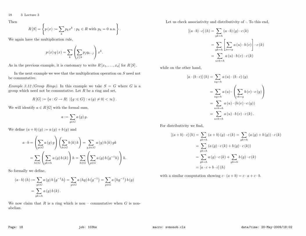
Let us check associativity and distributivity of ·. To this end,

[(a · b) · c] (h) =∑gk=h

(a · b) (g) · c (k)

=∑gk=h

[∑uv=g

a (u) · b (v)

]· c (k)

=∑uvk=h

a (u) · b (v) · c (k)

while on the other hand,

[a · (b · c)] (h) =∑uy=h

a (u) · (b · c) (y)

=∑uy=h

a (u) ·

∑vk=y

b (v) · c (y)

=∑uvk=h

a (u) · (b (v) · c (y))

=∑uvk=h

a (u) · b (v) · c (k) .

For distributivity we find,

[(a+ b) · c] (h) =∑gk=h

(a+ b) (g) · c (k) =∑gk=h

(a (g) + b (g)) · c (k)

=∑gk=h

(a (g) · c (k) + b (g) · c (k))

=∑gk=h

a (g) · c (k) +∑gk=h

b (g) · c (k)

= [a · c+ b · c] (h)

with a similar computation showing c · (a+ b) = c · a+ c · b.


4

Lecture 4

4.1 Units

Definition 4.1. Suppose R is a ring with identity. A unit of a ring is anelement a ∈ R such that there exists an element b ∈ R with ab = ba = 1. Welet U (R) ⊂ R denote the units of R.

Notice that in fact a = b in this definition since,

a = a · 1 = a (ub) = (au) b = 1 · b = b.

Moreover this argument shows that a satisfying au = 1 = ua is unique if itexists. For this reason we will write u−1 for a.

Proposition 4.2. The set U (R) equipped the multiplication law of R is a group.

Proof. This is a straight forward verification – see the homework assign-ment. The main point is to observe that u, v ∈ U (R) , then a := v−1u−1

satisfies, a (uv) = 1 = (uv) a, showing U (R) is closed under the multiplicationoperation of R.

Example 4.3. In M2(R), the units in this ring are exactly the elements inGL(2,R), i.e.

U (M2 (R)) = GL(2,R) = {A ∈M2 (R) : detA 6= 0} .

If you look back at last quarters notes you will see that we have alreadyproved the following theorem. I will repeat the proof here for completeness.

Theorem 4.4 (U (Zm) = U (m)). For any m ≥ 2,

U (Zm) = U (m) = {a ∈ {1, 2, . . . ,m− 1} : gcd (a,m) = 1} .

Proof. If a ∈ U (Zm) , there there exists r ∈ Zm such that 1 = r · a =ramodm. Equivalently put, m| (ra− 1) , i.e. there exists t such that ra − 1 =tm. Since 1 = ra− tm it follows that gcd (a,m) = 1, i.e. that a ∈ U (m) .

Conversely, if a ∈ U (m) ⇐⇒ gcd (a,m) = 1 which we know implies thereexists s, t ∈ Z such that sa + tm = 1. Taking this equation modm and lettingb := smodm ∈ Zm, we learn that b · a = 1 in Zm, i.e. a ∈ U (Zm) .

Example 4.5. In R, the units are exactly the elements in R× := R \ {0} that isU (R) = R×.

Example 4.6. Let R be the non-commutative ring of linear maps from R∞ toR∞ where

R∞ = {(a1, a2, a3, . . . ) : ai ∈ R for all i} ,

which is a vector space over R. Further let A,B ∈ R be defined by

A (a1, a2, a3, . . . ) = (0, a1, a2, a3, . . . ) andB (a1, a2, a3, . . . ) = (a2, a3, a4, . . . ) .

Then BA = 1 where

1 (a1, a2, a3, . . . ) = (a1, a2, a3, . . . )

whileAB (a1, a2, a3, . . . ) = (0, a2, a3, . . . ) 6= 1 (a1, a2, a3, . . . ) .

This shows that even though BA = 1 it is not necessarily true that AB = 1.Neither A nor B are units of R∞.

4.2 (Zero) Divisors and Integral Domains

Definition 4.7 (Divisors). Let R be a ring. We say that for elements a, b ∈ Rthat a divides b if there exists an element c such that ac = b.

Note that if R = Z then this is the usual notion of whether one integerevenly divides another, e.g., 2 divides 6 and 2 doesn’t divide 5.

Definition 4.8 (Zero divisors). A nonzero element a ∈ R is called a zerodivisor if there exists another nonzero element b ∈ R such that ab = 0, i.e. adivides 0 in a nontrivial way. (The trivial way for a|0 is; 0 = a ·0 as this alwaysholds.)

Definition 4.9 (Integral domain). A commutative ring R with no zero di-visors is called an integral domain (or just a domain). Alternatively put,R should satisfy, ab 6= 0 for all a, b ∈ R with a 6= 0 6= b.

20 4 Lecture 4

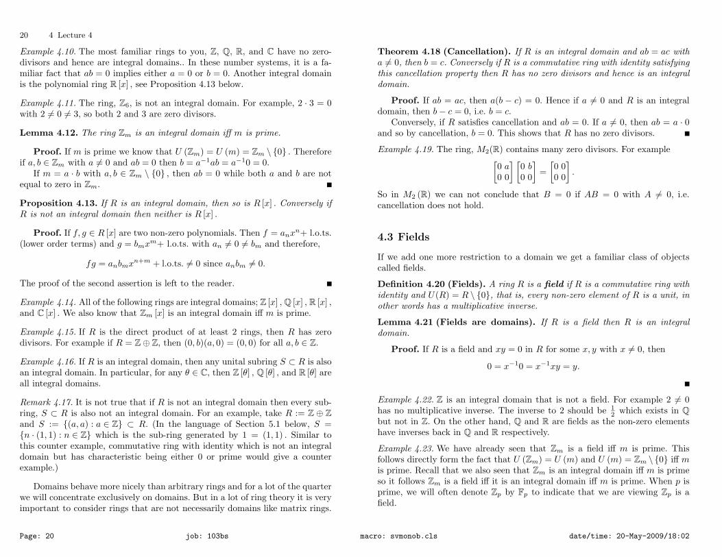
Example 4.10. The most familiar rings to you, Z, Q, R, and C have no zero-divisors and hence are integral domains.. In these number systems, it is a fa-miliar fact that ab = 0 implies either a = 0 or b = 0. Another integral domainis the polynomial ring R [x] , see Proposition 4.13 below.

Example 4.11. The ring, Z6, is not an integral domain. For example, 2 · 3 = 0with 2 6= 0 6= 3, so both 2 and 3 are zero divisors.

Lemma 4.12. The ring Zm is an integral domain iff m is prime.

Proof. If m is prime we know that U (Zm) = U (m) = Zm \ {0} . Thereforeif a, b ∈ Zm with a 6= 0 and ab = 0 then b = a−1ab = a−10 = 0.

If m = a · b with a, b ∈ Zm \ {0} , then ab = 0 while both a and b are notequal to zero in Zm.

Proposition 4.13. If R is an integral domain, then so is R [x] . Conversely ifR is not an integral domain then neither is R [x] .

Proof. If f, g ∈ R [x] are two non-zero polynomials. Then f = anxn+ l.o.ts.

(lower order terms) and g = bmxm+ l.o.ts. with an 6= 0 6= bm and therefore,

fg = anbmxn+m + l.o.ts. 6= 0 since anbm 6= 0.

The proof of the second assertion is left to the reader.

Example 4.14. All of the following rings are integral domains; Z [x] , Q [x] , R [x] ,and C [x] . We also know that Zm [x] is an integral domain iff m is prime.

Example 4.15. If R is the direct product of at least 2 rings, then R has zerodivisors. For example if R = Z⊕ Z, then (0, b)(a, 0) = (0, 0) for all a, b ∈ Z.

Example 4.16. If R is an integral domain, then any unital subring S ⊂ R is alsoan integral domain. In particular, for any θ ∈ C, then Z [θ] , Q [θ] , and R [θ] areall integral domains.

Remark 4.17. It is not true that if R is not an integral domain then every sub-ring, S ⊂ R is also not an integral domain. For an example, take R := Z ⊕ Zand S := {(a, a) : a ∈ Z} ⊂ R. (In the language of Section 5.1 below, S ={n · (1, 1) : n ∈ Z} which is the sub-ring generated by 1 = (1, 1) . Similar tothis counter example, commutative ring with identity which is not an integraldomain but has characteristic being either 0 or prime would give a counterexample.)

Domains behave more nicely than arbitrary rings and for a lot of the quarterwe will concentrate exclusively on domains. But in a lot of ring theory it is veryimportant to consider rings that are not necessarily domains like matrix rings.

Theorem 4.18 (Cancellation). If R is an integral domain and ab = ac witha 6= 0, then b = c. Conversely if R is a commutative ring with identity satisfyingthis cancellation property then R has no zero divisors and hence is an integraldomain.

Proof. If ab = ac, then a(b − c) = 0. Hence if a 6= 0 and R is an integraldomain, then b− c = 0, i.e. b = c.

Conversely, if R satisfies cancellation and ab = 0. If a 6= 0, then ab = a · 0and so by cancellation, b = 0. This shows that R has no zero divisors.

Example 4.19. The ring, M2(R) contains many zero divisors. For example[0 a0 0

] [0 b0 0

]=[0 00 0

].

So in M2 (R) we can not conclude that B = 0 if AB = 0 with A 6= 0, i.e.cancellation does not hold.

4.3 Fields

If we add one more restriction to a domain we get a familiar class of objectscalled fields.

Definition 4.20 (Fields). A ring R is a field if R is a commutative ring withidentity and U(R) = R \ {0}, that is, every non-zero element of R is a unit, inother words has a multiplicative inverse.

Lemma 4.21 (Fields are domains). If R is a field then R is an integraldomain.

Proof. If R is a field and xy = 0 in R for some x, y with x 6= 0, then

0 = x−10 = x−1xy = y.

Example 4.22. Z is an integral domain that is not a field. For example 2 6= 0has no multiplicative inverse. The inverse to 2 should be 1

2 which exists in Qbut not in Z. On the other hand, Q and R are fields as the non-zero elementshave inverses back in Q and R respectively.

Example 4.23. We have already seen that Zm is a field iff m is prime. Thisfollows directly form the fact that U (Zm) = U (m) and U (m) = Zm \ {0} iff mis prime. Recall that we also seen that Zm is an integral domain iff m is primeso it follows Zm is a field iff it is an integral domain iff m is prime. When p isprime, we will often denote Zp by Fp to indicate that we are viewing Zp is afield.


5

Lecture 5

In fact, there is another way we could have seen that Zp is a field, using thefollowing useful lemma.

Lemma 5.1. If R be an integral domain with finitely many elements, then Ris a field.

Proof. Let a ∈ R with a 6= 0. We need to find a multiplicative inverse fora. Consider a, a2, a3, . . . . Since R is finite, the elements on this list are not alldistinct. Suppose then that ai = aj for some i > j ≥ 1. Then ajai−j = aj · 1.By cancellation, since R is a domain, ai−j = 1. Then ai−j−1 is the inverse fora. Note that ai−j−1 ∈ R makes sense because i− j − 1 ≥ 0.

For general rings, an only makes sense for n ≥ 1. If 1 ∈ R and a ∈ U (R) ,we may define a0 = 1 and a−n =

(a−1

)n for n ∈ Z+. As for groups we thenhave anam = an+m for all m,n ∈ Z. makes sense for all n ∈ Z, but in generallynegative powers don’t always make sense in a ring. Here is another very inter-esting example of a field, different from the other examples we’ve written downso far.

Example 5.2. Lets check that C is a field. Given 0 6= a + bi ∈ C, a, b ∈ R,i =√−1, we need to find (a+ ib)−1 ∈ C. Working formally; we expect,

(a+ ib)−1 =1

a+ bi=

1a+ bi

a− bia− bi

a− bia2 + b2

=a

a2 + b2− b

a2 + b2i ∈ C,

which makes sense if N (a+ ib) := a2 + b2 6= 0, i.e. a+ ib 6= 0. A simple directcheck show that this formula indeed gives an inverse to a+ ib;

(a+ ib)[

a

a2 + b2− b

a2 + b2i

]=

1a2 + b2

(a+ ib) (a− ib) =1

a2 + b2(a2 + b2

)= 1.

So if a+ ib 6= 0 we have shown

(a+ bi)−1 =a

a2 + b2− b

a2 + b2i.

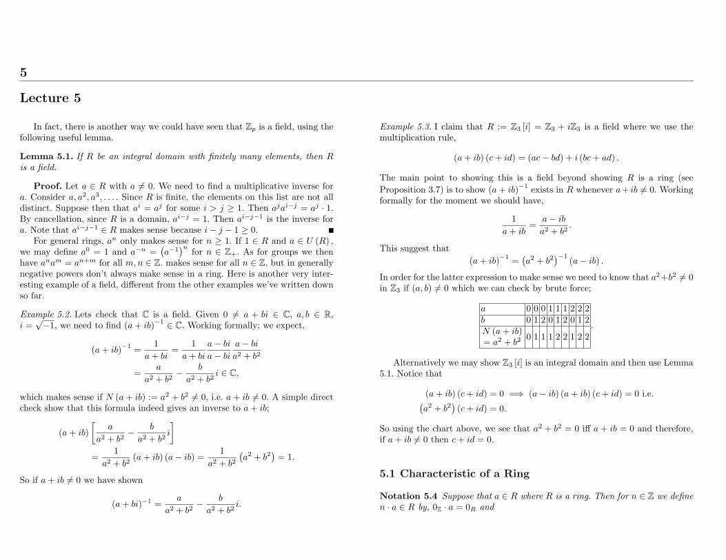
Example 5.3. I claim that R := Z3 [i] = Z3 + iZ3 is a field where we use themultiplication rule,

(a+ ib) (c+ id) = (ac− bd) + i (bc+ ad) .

The main point to showing this is a field beyond showing R is a ring (seeProposition 3.7) is to show (a+ ib)−1 exists in R whenever a+ ib 6= 0. Workingformally for the moment we should have,

1a+ ib

=a− iba2 + b2

.

This suggest that(a+ ib)−1 =

(a2 + b2

)−1(a− ib) .

In order for the latter expression to make sense we need to know that a2+b2 6= 0in Z3 if (a, b) 6= 0 which we can check by brute force;

a 0 0 0 1 1 1 2 2 2b 0 1 2 0 1 2 0 1 2N (a+ ib)= a2 + b2

0 1 1 1 2 2 1 2 2.

Alternatively we may show Z3 [i] is an integral domain and then use Lemma5.1. Notice that

(a+ ib) (c+ id) = 0 =⇒ (a− ib) (a+ ib) (c+ id) = 0 i.e.(a2 + b2

)(c+ id) = 0.

So using the chart above, we see that a2 + b2 = 0 iff a + ib = 0 and therefore,if a+ ib 6= 0 then c+ id = 0.

5.1 Characteristic of a Ring

Notation 5.4 Suppose that a ∈ R where R is a ring. Then for n ∈ Z we definen · a ∈ R by, 0Z · a = 0R and

22 5 Lecture 5

n · a =

n times︷︸︸︷

a+ · · ·+ a if n ≥ 1

−

|n| times︷︸︸︷(a+ · · ·+ a) = |n| · (−a) if n ≤ −1

.

So 3 · a = a+ a+ a while −2 · a = −a− a.

Lemma 5.5. Suppose that R is a ring and a, b ∈ R. Then for all m,n ∈ Z wehave

(m · a) b = m · (ab) , (5.1)a (m · b) = m · (ab) . (5.2)

We also have

− (m · a) = (−m) · a = m · (−a) and (5.3)m · (n · a) = mn · a. (5.4)

Proof. If m = 0 both sides of Eq. (5.1) are zero. If m ∈ Z+, then using thedistributive associativity laws repeatedly gives;

(m · a) b =

m times︷︸︸︷(a+ · · ·+ a)b

=

m times︷︸︸︷(ab+ · · ·+ ab) = m · (ab) .

If m < 0, then

(m · a) b = (|m| · (−a)) b = |m| · ((−a) b) = |m| · (−ab) = m · (ab)

which completes the proof of Eq. (5.1). The proof of Eq. (5.2) is similar andwill be omitted.

If m = 0 Eq. (5.3) holds. If m ≥ 1, then

− (m · a) = −m times︷︸︸︷

(a+ · · ·+ a) =

m times︷︸︸︷((−a) + · · ·+ (−a)) = m · (−a) = (−m) · a.

If m < 0, then

− (m · a) = − (|m| · (−a)) = (− |m|) · (−a) = m · (−a)

and

− (m · a) = − (|m| · (−a)) = (|m| · (− (−a))) = |m| · a = (−m) · a.

which proves Eq. (5.3).Letting x := sgn(m)sgn(n)a, we have

m · (n · a) = |m| · (|n| · x) =

|m| times︷︸︸︷(|n| · x+ · · ·+ |n| · x)

=

|m| times︷︸︸︷|n| times︷︸︸︷

(x+ · · ·+ x) + · · ·+

|n| times︷︸︸︷(x+ · · ·+ x)

= (|m| |n|) · x = mn · a.

Corollary 5.6. If R is a ring, a, b ∈ R, and m,n ∈ Z, then

(m · a) (n · b) = mn · ab. (5.5)

Proof. Using Lemma 5.5 gives;

(m · a) (n · b) = m · (a (n · b)) = m · (n · (ab)) = mn · ab.

Corollary 5.7. Suppose that R is a ring and a ∈ R. Then for all m,n ∈ Z,

(m · a) (n · a) = mn · a2.

In particular if a = 1 ∈ R we have,

(m · 1) (n · 1) = mn · 1.

Unlike the book, we will only bother to define the characteristic for ringswhich have an identity, 1 ∈ R.

Definition 5.8 (Characteristic of a ring). Let R be a ring with 1 ∈ R. Thecharacteristic, chr (R) , of R is is the order of the element 1 in the additivegroup (R,+). Thus n is the smallest number in Z+ such that n · 1 = 0. If nosuch n ∈ Z+ exists, we say that characteristic of R is 0 by convention and writechr (R) = 0.

Lemma 5.9. If R is a ring with identity and chr (R) = n ≥ 1, then n · x = 0for all x ∈ R.

Proof. For any x ∈ R, n · x = n · (1x) = (n · 1)x = 0x = 0.

Lemma 5.10. Let R be a domain. If n = chr (R) ≥ 1, then n is a primenumber.


Proof. If n is not prime, say n = pq with 1 < p < n and 1 < q < n, then

(p · 1R) (q · 1R) = pq · (1R1R) = pq · 1R = n · 1R = 0.

As p · 1R 6= 0 and q · 1R 6= 0 and we may conclude that both p · 1R and q · 1Rare zero divisors contradicting the assumption that R is an integral domain.

Example 5.11. The rings Q, R, C, Q[√

d]

:= Q+Q√d, Z [x] , Q [x] , R [x] , and

Z [x] all have characteristic 0.For each m ∈ Z+, Zm and Zm [x] are rings with characteristic m.

Example 5.12. For each prime, p, Fp := Zp is a field with characteristic p. Wealso know that Z3 [i] is a field with characteristic 3. Later, we will see otherexamples of fields of characteristic p.

6

Lecture 6

6.1 Square root field extensions of Q

Recall that√

2 is irrational. Indeed suppose that√

2 = m/n ∈ Q and, with outloss of generality, assume that gcd (m,n) = 1. Then m2 = 2n2 from which itfollows that 2|m2 and so 2|m by Euclid’s lemma. However, it now follows that22|2n2 and so 2|n2 which again by Euclid’s lemma implies 2|n. However, weassumed that m and n were relatively prime and so we have a contradictionand hence

√2 is indeed irrational. As a consequence of this fact, we know that{

1,√

2}

are linearly independent over Q, i.e. if a+ b√

2 = 0 then a = 0 = b.

Example 6.1. In this example we will show,

R = Q[√

2]

= {a+ b√

2 : a, b ∈ Q} (6.1)

is a field. Using similar techniques to those in Example 3.4 we see that Q[√

2]

may be described as in Eq. (6.1) and hence is a subring of Q by Proposition3.3. Alternatively one may check directly that the right side of Eq. (6.1) is asubring of Q since;

a+ b√

2− (c+ d√

2) = (a− c) + (b− d)√

2 ∈ R

and

(a+ b√

2)(c+ d√

2) = ac+ bc√

2 + ad√

2 + bd(2)

= (ac+ 2bd) + (bc+ ad)√

2 ∈ R.

So by either means we see that R is a ring and in fact an integral domain byExample 4.16. It does not have finitely many elements so we can’t use Lemma5.1 to show it is a field. However, we can find

(a+ b

√2)−1

directly as follows.

If ξ =(a+ b

√2)−1

, then1 = (a+ b

√2)ξ

and therefore,

a− b√

2 = (a− b√

2)(a+ b√

2)ξ =(a2 − 2b2

)ξ

which implies,

ξ =a

a2 − 2b2+

−ba2 − 2b2

√2 ∈ Q

[√2].

Moreover, it is easy to check this ξ works provided a2−2b2 6= 0. But if a2−2b2 =0 with b 6= 0, then

√2 = |a| / |b| showing

√2 is irrational which we know to be

false – see Proposition 6.2 below for details. Therefore, Q[√

2]

is a field.

Observe that Q ( R := Q[√

2]( R. Why is this? One reason is that

R := Q[√

2]

is countable and R is uncountable. Or it is not hard to show thatan irrational number selected more or less at random is not in R. For example,you could show that

√3 /∈ R. Indeed if

√3 = a+ b

√2 for some a, b ∈ Q then

3 = a2 + 2ab√

2 + 2b2

and hence 2ab√

2 = 3 − a2 − 2b2. Since√

2 is irrational, this can only happenif either a = 0 or b = 0. If b = 0 we will have

√3 ∈ Q which is false and if

a = 0 we will have 3 = 2b2. Writing b = kl , this with gcd (k, l) = 1, we find

3l2 = 2k2 and therefore 2|l by Gauss’ lemma. Hence 22|2k2 which implies 2|kand therefore gcd (k, l) ≥ 2 > 1 which is a contradiction. Hence it follows that√

3 6= a+ b√

2 for any a, b ∈ Q.The following proposition is a natural extension of Example 6.1.

Proposition 6.2. For all d ∈ Z \ {0} , F := Q[√

d]

is a field. (As we will seein the proof, we need only consider those d which are “square prime” free.

Proof. As F := Q[√

d]

= Q+Q√d is a subring of R which is an integral

domain, we know that F is again an integral domain. Let d = εpk11 . . . pknn

with ε ∈ {±1} , p1, . . . , pn being distinct primes, and ki ≥ 1. Further let δ =ε∏i:ki is odd pi, then

√d = m

√δ for some integer m and therefore it easily

follows that F = Q[√

δ]. So let us now write δ = εp1 . . . pk with ε ∈ {±1} ,

p1, . . . , pk being distinct primes so that δ is square prime free.Working as above we look for the inverse to a+ b

√δ when (a, b) 6= 0. Thus

we will look for u, v ∈ Q such that

1 =(a+ b

√δ)(

u+ v√δ).

Multiplying this equation through by a− b√δ shows,

26 6 Lecture 6

a− b√δ =

(a2 − b2δ

) (u+ v

√δ)

so thatu+ v

√δ =

a

a2 − b2δ− b

a2 − b2δ√δ. (6.2)

Thus we may define,(a+ b

√δ)−1

=a

a2 − b2δ− b

a2 − b2δ√δ

provided a2 − b2δ 6= 0 when (a, b) 6= (0, 0) .Case 1. If δ < 0 then a2 − b2δ = a2 + |δ| b2 = 0 iff a = 0 = b.Case 2. If δ ≥ 2 and suppose that a, b ∈ Q with a2 = b2δ. For sake of

contradiction suppose that b 6= 0. By multiplying a2 = b2δ though by thedenominators of a2 and b2 we learn there are integers, m,n ∈ Z+ such thatm2 = n2δ. By replacing m and n by m

gcd(m,n) and ngcd(m,n) , we may assume that

m and n are relatively prime.We now have p1|

(n2δ)

implies p1|m2 which by Euclid’s lemma implies thatp1|m. Thus we learn that p2

1|m2 = n2p1, . . . , pk and therefore that p1|n2. An-other application of Euclid’s lemma shows p1|n. Thus we have shown that p1 isa divisor of both m and n contradicting the fact that m and n were relativelyprime. Thus we must conclude that b = 0 = a. Therefore a2 − b2δ = 0 only ifa = 0 = b.

Later on we will show the following;

Fact 6.3 Suppose that θ ∈ C is the root of some polynomial in Q [x] , then Q [θ]is a sub-field of C.

Recall that we already know Q [θ] is an integral domain. To prove that Q [θ]is a field we will have to show that for every nonzero z ∈ Q [θ] that the inverse,z−1 ∈ C, is actually back in Q [θ] .

6.2 Homomorphisms

Definition 6.4. Let R and S be rings. A function ϕ : R→ S is a homomor-phism if

ϕ(r1r2) = ϕ(r1)ϕ(r2) andϕ(r1 + r2) = ϕ(r1) + ϕ(r2)

for all r1, r2 ∈ R. That is, ϕ preserves addition and multiplication. If we furtherassume that ϕ is an invertible map (i.e. one to one and onto), then we sayϕ : R→ S is an isomorphism and that R and S are isomorphic.

Example 6.5 (Conjugation isomorphism). Let ϕ : C→ C be defined by ϕ (z) =z where for z = x + iy, z := x − iy is the complex conjugate of z. Then it isroutine to check that ϕ is a ring isomorphism. Notice that z = z iff z ∈ R. Thereis analogous conjugation isomorphism on Q [i] , Z [i] , and Zm [i] (for m ∈ Z+)with similar properties.

Here is another example in the same spirit of the last example.

Example 6.6 (Another conjugation isomorphism). Let ϕ : Q[√

2]→ Q

[√2]

bedefined by

ϕ(a+ b

√2)

= a− b√

2 for all a, b ∈ Q.

Then ϕ is a ring isomorphism. Again this is routine to check. For example,

ϕ(a+ b

√2)ϕ(u+ v

√2)

=(a− b

√2)(

u− v√

2)

= au+ 2bv − (av + bu)√

2

while

ϕ((a+ b

√2)(

u+ v√

2))

= ϕ(au+ 2bv + (av + bu)

√2)

= au+ 2bv − (av + bu)√

2.

Notice that for ξ ∈ Q[√

2], ϕ (ξ) = ξ iff ξ ∈ Q.

Example 6.7. The only ring homomorphisms, ϕ : Z→ Z are ϕ (a) = a andϕ (a) = 0 for all a ∈ Z. Indeed, if ϕ : Z→ Z is a ring homomorphism andt := ϕ (1) , then t2 = ϕ (1)ϕ (1) = ϕ (1 · 1) = ϕ (1) = t. The only solutions tot2 = t in Z are t = 0 and t = 1. In the first case ϕ ≡ 0 and in the second ϕ = id.


7

Lecture 7

Example 7.1. Suppose that g ∈ M2 (R) is a unit, i.e. g−1 exists. Then ϕ :M2 (R)→M2 (R) defined by,

ϕ (A) := gAg−1 for all A ∈M2 (R) ,

is a ring isomorphism. For example,

ϕ (A)ϕ (B) =(gAg−1

) (gBg−1

)= gAg−1gBg−1 = gABg−1 = ϕ (AB) .

Observe that ϕ−1 (A) = g−1Ag and ϕ (I) = I.

Proposition 7.2 (Homomorphisms from Z). Suppose that R is a ring anda ∈ R is an element such that a2 = a. Then there exists a unique ring ho-momorphism, ϕ : Z → R such that ϕ (1) = a. Moreover, ϕ (k) = k · a for allk ∈ Z.

Proof. Recall from last quarter that, ϕ (n) := n · a for all n ∈ Z is a grouphomomorphism. This is also a ring homomorphism since,

ϕ (m)ϕ (n) = (m · a) (n · a) = mn · a2 = mn · a = ϕ (mn) ,

wherein we have used Corollary 5.6 for the second equality.

Corollary 7.3. Suppose that R is a ring with 1R ∈ R. Then there is a uniquehomomorphism, ϕ : Z→ R such that ϕ (1Z) = 1R.

Proposition 7.4. Suppose that ϕ : R→ S is a ring homomorphism. Then;

1. ϕ (0) = 0,2. ϕ (−r) = −ϕ (r) for all r ∈ R,3. ϕ(r1 − r2) = ϕ(r1)− ϕ(r2) for all r1, r2 ∈ R.4. If 1R ∈ R and ϕ is surjective, then ϕ (1R) is an identity in S.5. If ϕ : R → S is an isomorphism of rings, then ϕ−1 : S → R is also a

isomorphism.

Proof. Noting that ϕ : (R,+)→ (S,+) is a group homomorphism, it followsthat items 1. – 3. were covered last quarter when we studied groups. The proofof item 5. is similar to the analogous statements for groups and hence will beomitted. So let me prove item 4. here.

To each s ∈ S, there exists a ∈ R such that ϕ (a) = s. Therefore,

ϕ (1R) s = ϕ (1R)ϕ (a) = ϕ (1Ra) = ϕ (a) = s

andsϕ (1R) = ϕ (a)ϕ (1R) = ϕ (a1R) = ϕ (a) = s.

Since these equations hold for all s ∈ S, it follows that ϕ (1R) is an (the) identityin S.

Definition 7.5. As usual, if ϕ : R→ S is a ring homomorphism we let

ker (ϕ) := {r ∈ R : ϕ (r) = 0} = ϕ−1 ({0S}) ⊂ R.

Lemma 7.6. If ϕ : R→ S is a ring homomorphism, then ker (ϕ) is an ideal ofR.

Proof. We know from last quarter that ker (ϕ) is a subgroup of (R,+) . Ifr ∈ R and n ∈ ker (ϕ) , then

ϕ (rn) = ϕ (r)ϕ (n) = ϕ (r) 0 = 0 andϕ (nr) = ϕ (n)ϕ (r) = 0ϕ (r) = 0,

which shows that rn and nr ∈ ker (ϕ) for all r ∈ R and n ∈ ker (ϕ) .

Example 7.7. Let us find all of the ring homomorphisms, ϕ : Z→ Z10 and theirkernels. To do this let t := ϕ (1) . Then t2 = ϕ (1)ϕ (1) = ϕ (1 · 1) = ϕ (1) = t.The only solutions to t2 = t in Z10 are t = 0, t = 1, t = 5 and t = 6.

1. If t = 0, then ϕ ≡ 0 and ker (ϕ) = Z.2. If t = 1, then ϕ (x) = xmod 10 and kerϕ = 〈10〉 = 〈0〉 = {0} ⊂ Z.3. If t = 5, then ϕ (x) = 5xmod 10 and x ∈ kerϕ iff 10|5x iff 2|x so that

ker (ϕ) = 〈2〉 = {0, 2, 4, 8} .4. If t = 6, then ϕ (x) = 6xmod 10 and x ∈ kerϕ iff 10|6x iff 5|x so that

ker (ϕ) = 〈5〉 = {0, 5} ⊂ Z.

Proposition 7.8. Suppose n ∈ Z+, R is a ring, and a ∈ R is an element suchthat a2 = a and n · a = 0. Then there is a unique homomorphism, ϕ : Zn → Rsuch that ϕ (1) = a and in fact ϕ (k) = k · a for all k ∈ Zn.

28 7 Lecture 7

Proof. This has a similar proof to the proof of Proposition 7.2.

Corollary 7.9. Suppose that R is a ring, 1R ∈ R, and chr (R) = n ∈ Z+. Thenthere is a unique homomorphism, ϕ : Zn → R such that ϕ (1Zn

) = 1R which isgiven by ϕ (m) = m · 1R for all m ∈ Zn. Moreover, ker (ϕ) = 〈0〉 = {0} .

Example 7.10. Suppose that ϕ : Z10 → Z10 is a ring homomorphism and t :=ϕ (1) . Then t2 = ϕ (1)2 = ϕ (1) = t, and therefore t2 = t. Moreover we musthave 0 = ϕ (0) = ϕ (10 · 1) = 10 · t which is not restriction on t. As we haveseen the only solutions to t2 = t in Z10 are t = 0, t = 1, t = 5 and t = 6. Thusϕ must be one of the following; ϕ ≡ 0, ϕ = id, ϕ (x) = 5x, or ϕ (x) = 6x for allx ∈ Z10. The only ring isomorphism is the identity in this case. If ϕ (x) = 5x

Example 7.11. Suppose that ϕ : Z12 → Z10 is a ring homomorphism and lett := ϕ (1). Then as before, t2 = t and this forces t = 0, 1, 5, or 6. In this casewe must also require 12 · t = 0, i.e. 10|12 · t, i.e. 5|t. Therefore we may now onlytake t = 0 or t = 5, i.e.

ϕ (x) = 0 for all x ∈ Z12 orϕ (x) = 5xmod 10 for all x ∈ Z12

are the only such homomorphisms.

Theorem 7.12 (Not covered in class). If ϕ : R→ R is a ring homomor-phism, then ϕ is either the zero or the identity homomorphism.

Proof. If t = ϕ (1) , then as above, t2 = t, i.e. t (t− 1) = 0. Since R is afield this implies that t = 0 or t = 1. If t = 0, then for all a ∈ R,

ϕ (a) = ϕ (a · 1) = ϕ (a)ϕ (1) = ϕ (a) · 0 = 0,

i.e. ϕ is the zero homomorphism. So we may now assume that t = 1.If t = 1,

ϕ (n) = ϕ (n · 1) = n · ϕ (1) = n · 1 = n

for all n ∈ Z. Therefore for n ∈ N \ {0} and m ∈ Z,

m = ϕ (m) = ϕ(n · m

n

)= ϕ (n)ϕ

(mn

)= nϕ

(mn

)from which it follows that ϕ (m/n) = m/n. Thus we now know that ϕ|Q is theidentity.

Since ker (ϕ) 6= R, we must have ker (ϕ) = {0} so that ϕ is injective. Inparticular ϕ (b) 6= 0 for all b 6= 0. Moreover if a > 0 in R and b :=

√a, then

ϕ (a) = ϕ(b2)

= [ϕ (b)]2 > 0.

So if y, x ∈ R with y > x, then ϕ (y) − ϕ (x) = ϕ (y − x) > 0, i.e. ϕ is orderpreserving.

Finally, let a ∈ R and choose rational numbers xn, yn ∈ Q such that xn <a < yn with xn ↑ a and yn ↓ a as n→∞. Then

xn = ϕ (xn) < ϕ (a) < ϕ (yn) = yn for all n.

Letting n → ∞ in this last equation then shows, a ≤ ϕ (a) ≤ a, i.e. ϕ (a) = a.Since a ∈ R was arbitrary, we may conclude that ϕ is the identity map on R.


8

Lecture 8

Remark 8.1 (Comments on ideals). Let me make two comments on ideals in acommutative ring, R.

1. To check that a non-empty subset, S ⊂ R, is an ideal, we should show(S,+) is a subgroup of R and that RS ⊂ S. Since R is commutative, youdo not have to also show SR ⊂ S. This is because RS = SR in when R iscommutative.

2. If a ∈ R, the principle ideal generated by a is defined by;

〈a〉 := Ra = {ra : r ∈ R} .

It is easy to check that this is indeed an ideal. So for example if R = R [x]then 〈x〉 = R [x] ·x which is the same as the polynomials without a constantterm, i.e. p (x) = a1x+ a2x

2 + · · ·+ anxn. The coefficient a0 = 0. Similarly,⟨

x2 + 1⟩

= R [x](x2 + 1

)is the collection of all polynomials which contain(

x2 + 1)

as a factor.

Recall from last time:

1. If a ∈ R satisfies a2 = a, then ϕ (k) := k · a is a ring homomorphism fromZ→ R.

2. If we further assume that n · a = 0 for some n ∈ Z+, then ϕ (k) := k · a alsodefines a ring homomorphism from Zn → R.

Example 8.2. For any m > 1, ϕ : Z → Zm given by ϕ (a) = a · 1Zm = amodmis a ring homomorphism. This also follows directly from the properties of the(·) modm – function. In this case ker (ϕ) = 〈m〉 = Zm.

Example 8.3. If n ∈ Z+ and m = kn with k ∈ Z+, then there is a unique ringhomomorphisms, ϕ : Zm → Zn such that ϕ (1m) = 1n. To be more explicit,

ϕ (a) = ϕ (a · 1m) = a · ϕ (1m) = a · 1n = (amodn) · 1n = amodn.

Example 8.4. In Z10, the equation, a2 = a has a solutions a = 5 and a = 6.Notice that |5| = 2 and |6| = |gcd (10, 6)| = |2| = 5. Thus we know that for anyk ≥ 1 there are ring homomorphisms, ϕ : Z5k → Z10 and ψ : Z2k → Z10 suchthat

ϕ (15k) = 6 and ψ (12k) = 5.

As before, one shows that

ϕ (m) = m · 6 = (6m) mod 10 and ψ (m) = m · 5 = (5m) mod 10.

Example 8.5 (Divisibility tests). Let n = akak−1 . . . a0 be written in decimalform, so that

n =k∑i=0

ai10i. (8.1)

Applying the ring homomorphism, mod 3 and mod 9 to this equation shows,

nmod 3 =k∑i=0

ai mod 3 · (10 mod 3)i

=

(k∑i=0

ai

)mod 3

and similarly,

nmod 9 =k∑i=0

ai mod 9 · (10 mod 9)i =

(k∑i=0

ai

)mod 9.

Thus we learn that nmod 3 = 0 iff(∑k

i=0 ai

)mod 3 = 0 i.e. 3|n iff

3|(∑k

i=0 ai

). Similarly, since 10 mod 9 = 1, the same methods show 9|n iff

9|(∑k

i=0 ai

). (See the homework problems for more divisibility tests along

these lines. Also consider what this test gives if you apply mod 2 to Eq. (8.1).)

Theorem 8.6. Let R be a commutative ring with 1 ∈ R. To each a ∈ R witha2 + 1 = 0, there is a unique ring homomorphism ϕ : Z [i] → R such thatϕ (1) = 1 and ϕ (i) = a.

Proof. Since Z [i] is generated by i, we see that ϕ is completely determinedby a := ϕ (i) ∈ R. Now we can not choose a arbitrarily since we must have

a2 = ϕ (i)2 = ϕ(i2)

= ϕ (−1) = −1R,

i.e. a2 + 1 = 0.Conversely given a ∈ R such that a2 + 1 = 0, we should define

ϕ (x+ iy) = x1 + ya for all x, y ∈ Z,where ya = a + a + · · · + a – y times. The main point in checking that ϕ is ahomomorphism is to show it preserves the multiplication operation of the rings.To check this, let x, y, u, v ∈ Z and consider;

ϕ ((x+ iy) (u+ iv)) = ϕ (xu− yv + i (xv + yu)) = (xu− yv) 1R + (xv + yu) a.

On the other hand

ϕ (x+ iy)ϕ (u+ iv) = (x1R + ya) (u1R + va)= (x1R + ya) (u1R + va)

= xu1R + yva2 + yua+ xva

= (xu− yv) 1R + (yu+ xv) a= ϕ ((x+ iy) (u+ iv)) .

Thus we have shown ϕ (ξη) = ϕ (ξ)ϕ (η) for all ξ, η ∈ Z [i] . The fact thatϕ (ξ + η) = ϕ (ξ) + ϕ (η) is easy to check and is left to the reader.

Remark 8.7. This could be generalized by supposing that a, b ∈ R with b2 = band a2 + b = 0. Then we would have ϕ (x+ yi) = x · b + y · a would be thedesired homomorphism. Indeed, let us observe that

ϕ (x+ iy)ϕ (u+ iv) = (xb+ ya) (ub+ va)= (xb+ ya) (ub+ va)

= xub2 + yva2 + yua+ xva

= (xu− yv) b+ (yu+ xv) a= ϕ ((x+ iy) (u+ iv)) .

Example 8.8. Let ϕ : Z [i] → Z3 [i] be the unique homomorphism such thatϕ (1) = 1 and ϕ (i) = i, i.e.

ϕ (a+ ib) = a · 1 + b · i = amod 3 + (bmod 3) i ∈ Z3 [i] .

Notice that

ker (ϕ) = {a+ bi : a, b ∈ 〈3〉 ⊂ Z} = 〈3〉+ 〈3〉 i.Here is a more interesting example.

Example 8.9. In Z10 we observe that 32 = 9 = −1 and also 7 = −3 has thisproperty, namely 72 = (−3)2 = 32 = 9 = −1. Therefore there exists a uniquehomomorphism, ϕ : Z [i] → Z10 such that ϕ (1) = 1 and ϕ (i) = 7 = −3. Theexplicit formula is easy to deduce,

ϕ (a+ bi) = a · 1 + b · 7 = (a− 3b) mod 10.

9

Lecture 9

Lemma 9.1. If ϕ : R→ S is a ring homomorphism, then ker (ϕ) is an ideal ofR.

Proof. We know from last quarter that ker (ϕ) is a subgroup of (R,+) . Ifr ∈ R and n ∈ ker (ϕ) , then

ϕ (rn) = ϕ (r)ϕ (n) = ϕ (r) 0 = 0 andϕ (nr) = ϕ (n)ϕ (r) = 0ϕ (r) = 0,

which shows that rn and nr ∈ ker (ϕ) for all r ∈ R and n ∈ ker (ϕ) .

Example 9.2. If ϕ : Z→ Zm is the ring homomorphism defined by ϕ (a) :=amodm, then

kerϕ = {a ∈ Z : amodm = 0} = Zm = 〈m〉 .

We will see many more examples of Lemma 9.1 below.

9.1 Factor Rings

Definition 9.3. Let R be a ring, I ⊂ R an ideal. The factor ring R/I is definedto be

R/I := {r + I : r ∈ R}

with operations

(a+ I) + (b+ I) := (a+ b) + I and(a+ I)(b+ I) := (ab) + I.

We may also write [a] for a+ I in which cases the above equations become,

[a] + [b] := [a+ b] and [a] [b] := [ab] .

Theorem 9.4. A factor ring really is a ring.

Proof. The elements of R/I are the left cosets of I in the group (R,+).There is nothing new here. R/I is itself a group with the operation + definedby (a + I) + (b + I) = (a + b) + I. This follows from last quarter as I ⊂ R isa normal subgroup of (R,+) since (R,+) is abelian. So we only need really tocheck that the definition of product makes sense.

Problem: we are multiplying coset representatives. We have to check thatthe resulting coset is independent of the choice of representatives. Thus weneed to show; if a, b, a′, b′ ∈ R with

a+ I = a′ + I and b+ I = b′ + I,

then ab + I = a′b′ + I. By definition of cosets, we have i := a − a′ ∈ I andj := b− b′ ∈ I. Therefore,

ab = (a′ + i) (b′ + j) = a′b′ + ib′ + a′j + ij ∈ a′b′ + I

since ib′+a′j+ ij ∈ I because I is an ideal. So indeed, ab+ I = a′b′+ I and wehave a well defined product on R/I. Checking that product is associative andthe distributive laws is easy and will be omitted.

Example 9.5. Suppose that I = 〈4〉 = Z · 4 ⊂ Z. In this case, if a ∈ Z thena− amod 4 ∈ I and therefore,

[a] = a+ I = amod 4 + I = [amod 4] .

Moreover if 0 ≤ a, b ≤ 3 with a + I = b + I then a − b ∈ I, i.e. a − b is amultiple of 4. Since |a− b| < 4, this is only possible if a = b. Thus if we letS = {0, 1, 2, 3} , then

Z/ 〈4〉 = {[m] = m+ 〈4〉 : m ∈ S} = [S] .

Moreover, we have[a] [b] = [ab] = [(ab) mod 4]

and[a] + [b] = [a+ b] = [(a+ b) mod 4] .

Thus the induced ring structure on S is precisely that of Z4 and so we mayconclude;

Z4 3 a→ [a] = a+ 〈4〉 ∈ Z/ 〈4〉is a ring isomorphism.

10

Lecture 10

Remark 10.1. Roughly speaking, you should think of R/I being R with theproviso that we identify two elements of R to be the same if they differ by anelement from I. To understand R/I in more concrete terms, it is often usefulto look for subset, S ⊂ R, such that the map,

S 3 a→ a+ I ∈ R/I

is a bijection. (We will call such an S a slice.) This allows us to identify R/Iwith S and this identification induces a ring structure on S. We will see howthis goes in the examples below. Warning: the choice of a slice S is highlynon-unique although there is often a “natural” choice in a given example. Thepoint is to make S we need only choose one element from each of the cosets inR/I.

Example 9.5 easily generalizes to give the following theorem. We will giveanother proof shortly using the first isomorphism theorem, see 10.4 below.

Theorem 10.2 (Zm ∼= Z/ 〈m〉). For all m ≥ 2, the map,

Zm 3 a→ [a] = a+ 〈m〉 ∈ Z/ 〈m〉 (10.1)

is a ring isomorphism.

Proof. The distinct cosets of Z/ 〈m〉 are given by

{[k] = k + 〈m〉 : k = 0, 1, 2 . . . ,m− 1}

and therefore we may take S = Zm. Since [a] = [amodm] , it is easy to see thatthe map in Eq. (10.1) is a ring isomorphism.

10.1 First Isomorphism Theorem

Recall that two rings, R and S (written R ∼= S) are isomorphic, if there is aring isomorphism, ϕ : R → S. That is ϕ should be a one-to-one and onto ringhomomorphism.

Theorem 10.3 (First Isomorphism Theorem). Let R and S be rings andϕ : R→ S be a homomorphism. Let

ϕ(R) = Ranϕ = {ϕ(r) : r ∈ R} ⊂ S

and recall that I = kerϕ := {r ∈ R : ϕ(r) = 0} is an ideal in R. Then ϕ(R) isa subring of S and ϕ : R/I → ϕ(R) defined by

ϕ ([r]) = ϕ (r + I) := ϕ (r) for all r ∈ R


Proof. We have seen last quarter that ϕ : R/ kerϕ→ ϕ(R) is an (additive)group isomorphism. So it only remains to show ϕ preserves the multiplicationoperations on ϕ (R) and R/I which goes as follows;

ϕ ([a]) ϕ ([b]) = ϕ (a)ϕ (b)= ϕ (ab) = ϕ ([ab]) = ϕ ([a] [b]) .

Example 10.4 (Z/ (Zm) ∼= Zm). Let m ∈ Z+ and ϕ : Z → Zm be the ringhomomorphism, ϕ (x) = xmodm. Since ϕ (Z) = Zm and ker (ϕ) = 〈m〉 = Zm,the first isomorphism theorem implies, ϕ : Z/ (Zm)→ Zm is a ring isomorphismwhere ϕ ([a]) = ϕ (a) = amodm for all a ∈ Z.

Example 10.5. Let us consider R := Z [i] / 〈i− 2〉 . In this ring [i− 2] = 0 orequivalently, [i] = [2] . Squaring this equation also shows,

[−1] =[i2]

= [i]2 = [2]2 =[22]

= [4]

from which we conclude that [5] = 0, i.e. 5 ∈ 〈i− 2〉 . This can also be seendirectly since 5 = − (i+ 2) (i− 2) ∈ 〈i− 2〉 . Using these observations we learnfor a+ ib ∈ Z [i] that

[a+ ib] = [a+ 2b] = [(a+ 2b) mod 5] .

Thus, if we define S = {0, 1, 2, 3, 4} , we have already shown that

R = {[a] : a ∈ S} = [S] .

Now suppose that a, b ∈ S with [a] = [b] , i.e. 0 = [a− b] = [c] wherec = (a− b) mod 5. Since c ∈ 〈i− 2〉 we must have

c = (i− 2) (a+ bi) = − (2a+ b) + (a− 2b) i

from which it follows that a = 2b and

c = − (2a+ b) = −5b.

Since 0 ≤ c < 5, this is only possible if c = 0 and therefore,

a = amod 5 = bmod 5 = b.

Finally let us now observe that

[a] + [b] = [a+ b] = [(a+ b) mod 5] and[a] · [b] = [ab] = [(ab) mod 5]

so that the induced ring structure on S is the same a the ring structure on Z5.Hence we have proved,

Z5 3 a→ [a] = a+ 〈i− 2〉 ∈ Z [i] / 〈i− 2〉

is an isomorphism of rings.

11

Lecture 11

Example 11.1 (Example 10.5 revisited). In Z5, we see that 22 = 4 = −1 andtherefore there is a ring homomorphism, ϕ : Z [i]→ Z5 such that ϕ (1) = 1 andϕ (i) = 2. More explicitly we have,

ϕ (a+ bi) = a · 1 + b · 2 = (a+ 2b) mod 5.

Moreover, (a+ ib) ∈ ker (ϕ) iff a+ 2b = 5k for some k ∈ Z and therefore,

ker (ϕ) = {−2b+ 5k + ib : b, k ∈ Z} = Z (2− i) + Z · 5.

Since (2 + i) (2− i) = 5 and 2− i ∈ ker (ϕ) , we have, and

〈2− i〉 ⊂ ker (ϕ) = Z (2− i) + Z · 5 ⊂ 〈2− i〉

from which it follows that ker (ϕ) = 〈2− i〉 . Thus by the first isomorphismtheorem, ϕ : Z [i] / 〈2− i〉 → Z5 defined by

ϕ ([a+ ib]) = ϕ (a+ bi) = (a+ 2b) mod 5

is a ring isomorphism. Notice that the inverse isomorphism is given by ϕ−1 (a) =[a] for all a ∈ Z5 which should be compared with Example 10.5 above.

For what follows recall that the evaluation maps are homomorphisms.

Theorem 11.2 (Evaluation homomorphism). Let R be a subring of acommutative ring, R, and t ∈ R. Then there exists a ring homomorphism,ϕt : R [x]→ R such that

ϕt (p) =n∑k=0

aktk when p (x) =

n∑k=0

akxk ∈ R [x] .

We will usually simply write p (t) for ϕt (p) .

The hole point of how we define polynomial multiplication is to make thistheorem true. We will give the formal proof of this theorem a bit later in thenotes.

Example 11.3. Let I := 〈x〉 = R [x]x ⊂ R [x] from which it follows that [x] =0 ∈ R [x] / 〈x〉 . Therefore if p (x) = a0 + a1x+ · · ·+ anx

n, then

[p (x)] = [a0 + a1x+ · · ·+ anxn] = [a0] .

Alternatively put, p (x) + I = a0 + I since a1x + · · · + anxn ∈ I. Moreover, if

[a0] = [b0] , then a0 − b0 ∈ I which can happen iff a0 = b0. Therefore we mayidentify R [x] / 〈x〉 with S = R thought of as the constant polynomials inside ofR [x] . In fact it is easy to check that

R 3 a→ a+ I ∈ R [x] / 〈x〉

is a ring isomorphism.Alternatively we may use the first isomorphism theorem as follows. Let

ϕ (p) := p (0) , then ϕ : R [x]→ R is a ring homomorphism onto R with ker (ϕ) =〈x〉 . Therefore, ϕ : R [x] / 〈x〉 → R is a ring isomorphism.

Theorem 11.4 (Division Algorithm). Let F [x] be a polynomial ring whereF is a field. Given f, g ∈ F [x] both nonzero, there exists a unique q, r ∈ F [x]with f = qg + r such that either r = 0 or deg r < deg g.

Interpretation. We are dividing f by g and so g goes into f, q timeswith remainder r. This is really high school polynomial division which wewill discuss in more detail a bit later. In the sequel we will sometimes denotethe remainder, r by f mod g.

Corollary 11.5. Suppose that F is a field, p (x) = c0 + · · ·+ cnxn ∈ F [x] is a

polynomial with cn 6= 0, and let

S :={a0 + a1x+ · · ·+ an−1x

n−1 : ai ∈ F for i = 0, 1, . . . , n− 1}.

Then the map, ϕ : S → F [x] / 〈p〉 defined by

ϕ (f) = [f ] := f + 〈p〉 for all f ∈ S

is a bijection. Moreover, S becomes a ring and ϕ a ring homomorphism providedwe define

f (x) · g (x) := [f (x) g (x)] mod p

and f + g as usual polynomial addition.

36 11 Lecture 11

Proof. 1. If f ∈ F [x] , then by the division algorithm

f = qp+ r = qp+ f mod p

and therefore,

[f ] = [qp+ r] = [q] [p] + [r] = [q] 0 + [r] = [r] .

Thus we have shown

[f ] = [f mod p] for all f ∈ F [x] . (11.1)

2. Equation (11.1) shows ϕ : S → F [x] / 〈p〉 is onto. To see ϕ is injective,suppose that f, g ∈ S and ϕ (f) = ϕ (g) . Then [f − g] = 0, i.e. f − g ∈ 〈p〉 , i.e.f − g = q · p for some q ∈ F [x] . However this is impossible unless q = 0 andf = g since otherwise,

n− 1 ≥ deg (f − g) = deg (q) + deg (p) = deg (q) + n.

Thus we have shown ϕ is injective as well, i.e. ϕ : S → F [x] / 〈p〉 is a bijection.3. Making use of Eq. (11.1) and the fact that ϕ is a bijection shows,

ϕ (f)ϕ (g) = [f ] [g] = [fg] = [(fg) mod p] = ϕ ((fg) mod p) andϕ (f) + ϕ (g) = [f ] + [g] = [f + g] = ϕ (f + g)

for all f, g ∈ S. Thus S equipped with the operations described in the theoremmakes S into a ring for which ϕ is a ring isomorphism.

Theorem 11.6 (C as a factor ring). C ∼= R [x] /⟨x2 + 1

⟩=: R. The maps,

C3 (a+ ib)→ [a+ bx] ∈ R [x] /⟨x2 + 1

⟩and

R [x] /⟨x2 + 1

⟩3 [p (x)] = p (x) +

⟨x2 + 1

⟩→ p (i) ∈ C

are ring isomorphisms which are inverses to one another.

Proof. We are going to give two proofs that C ∼= R [x] /⟨x2 + 1

⟩. Our first

proof gives rise to the first map while our second gives rise to the second map.First Proof. Let S = {a+ bx : x, b ∈ R} so that

S 3 (a+ bx)→ [a+ bx] ∈ R [x] /⟨x2 + 1

⟩is a bijection. Since

[x2 + 1

]= 0, we have

[x2]

= [−1] and therefore,

[a+ bx] [c+ dx] =[ac+ (bc+ ad)x+ bdx2

]= [ac+ (bc+ ad)x+ bd (−1)]= [ac− bd+ (bc+ ad)x] .

Moreover one easily shows,

[a+ bx] + [c+ dx] = [(a+ c) + (b+ d)x] .

From these two facts it is now easy to check that

C 3 (a+ ib)→ [a+ bx] ∈ R

is an isomorphism of rings.Second Proof. Let ϕ : R [x] → C be the evaluation homomorphism,

ϕ (p) = p (i) where i =√−1 ∈ C. We then have ϕ (R [x]) = R [i] = C and so

by the first isomorphism theorem, R [x] / ker (ϕ) ∼= C. So to finish the proof wemust show,

ker (ϕ) =⟨x2 + 1

⟩= R [x]

(x2 + 1

). (11.2)

Suppose that p ∈ ker (ϕ) and use the division algorithm to write,

p (x) = q (x)(x2 + 1

)+ r (x) where

r (x) = a+ bx for some a, b ∈ R.

As p (i) = 0 and i2 + 1 = 0, it follows that r (i) = a+ bi = 0. But this happensiff a = 0 = b, and therefore we see that r ≡ 0 an hence that p (x) ∈

⟨x2 + 1

⟩.

Thus we have shown ker (ϕ) ⊂⟨x2 + 1

⟩and since x2 + 1 ∈ ker (ϕ) we must

have ker (ϕ) =⟨x2 + 1

⟩which completes the second proof of the theorem.

Alternative method for computing ker (ϕ) .If p ∈ ker (ϕ) , then p (i) = 0. Taking the complex conjugates of this equation

(using z + w = z + w and zw = z · w for all z, w ∈ C) we learn that p (−i) = 0as well. As we will see in detail later, p (i) = 0 implies p (x) = (x− i)u (x) forsome u ∈ C [x] . Moreover since,

0 = p (−i) = −2i · u (−i)

we learn that u (−i) = 0 and therefore, u (x) = (x+ i) q (x) with q ∈ C [x] .Therefore,

p (x) = (x− i) (x+ i) q (x) =(x2 + 1

)q (x) .

It is not too hard to see (use complex conjugation again) that in fact q ∈ R [x] .Conversely if p (x) =

(x2 + 1

)q (x) with q ∈ R [x] , then p (i) = 0. Therefore we

have again proved Eq. (11.2).


12

Lecture 12

Example 12.1. Let R := Q [x] /⟨x2 − 2

⟩so that

[x2]

= [2] now. Again we takeS = {a+ bx : a, b ∈ Q} and observe that

[a+ bx] [c+ dx] =[ac+ (bc+ ad)x+ bdx2

]= [ac+ (bc+ ad)x+ bd2]= [ac+ 2bd+ (bc+ ad)x] .

Recalling that, in Q[√

2], that(

a+ b√

2)(

c+ d√

2)

= ac+ 2bd+ (bc+ ad)√

2

it follows that

Q[√

2]3 a+ b

√2→ [a+ bx] ∈ Q [x] /

⟨x2 − 2

⟩is a ring isomorphism.

Example 12.2 (Example 12.1 revisited). Let ϕ : Q [x] → Q[√

2]

be the eval-uation map, ϕ (p) = p

(√2). Then by the first isomorphism theorem, ϕ :

Q [x] / ker (ϕ)→ Q[√

2]

is an isomorphism of rings. We now claim that

ker (ϕ) =⟨x2 − 2

⟩. (12.1)

Since x2−2 ∈ ker (ϕ) we know that⟨x2 − 2

⟩⊂ ker (ϕ) . Conversely, if p ∈ ker (ϕ)

and p (x) = q (x)(x2 − 2

)+ r (x) for some r (x) = a+ bx with a, b ∈ Q, then

0 = p(√

2)

= q(√

2)· 0 + r

(√2)

= a+ b√

2.

As√

2 is irrational, this is only possible if a = b = 0, i.e. r (x) = 0. Thus wehave shown p ∈

⟨x2 − 2

⟩and therefore Eq. (12.1) is valid.

Example 12.3. Let I :=⟨x2⟩

= R [x]x2 ⊂ R [x] . If p (x) = a0 +a1x+ · · ·+anxn,then p + I = a0 + a1x + I since a2x

2 + · · · + anxn ∈ I. Alternatively, we now

have[x2]

= 0 in R [x] /⟨x2⟩, so that

[p (x)] = [a0 + a1x+ · · ·+ anxn] = [a0 + a1x] .

Moreover [a0 + a1x] = 0 iff a0 = a1 = 0, so we may take S ={a0 + a1x : a0, a1 ∈ R} – the polynomials of degree less than or equal to 1.Thus it follows that

R [x] /⟨x2⟩

= {(a0 + a1x) + I : a0, a1 ∈ R} ∼ R2.

This induces a ring multiplication on R2 determined as follows;

[a0 + a1x] [b0 + b1x] = [(a0 + a1x) (b0 + b1x)]

=[a0b0 + (a1b0 + a0b1)x+ a1b1x

2]

= [a0b0 + (a1b0 + a0b1)x] .

Thus the multiplication rule on S should be defined by

(a0 + a1x) (b0 + b1x) = a0b0 + (a1b0 + a0b1)x.

Alternatively, if we identify S with R := R2 and equip R with the multiplicationand addition rules,

(a0, a1) · (b0, b1) = (a0b0, a1b0 + a0b1) and (12.2)(a0, a1) + (b0, b1) = (a0 + b0, a1 + b1) ,

thenR 3 (a0, a1)→ a0 + a1x+ I ∈ R [x] /

⟨x2⟩


An important point to observe for later is that R in Example 12.3 is not afield and in fact not even an integral domain. For example, (0, 1)·(0, 1) = (0, 0) =0. Alternatively, notice that [x] · [x] =

[x2]

= 0, so that 0 6= [x] ∈ R [x] /⟨x2⟩

isa zero divisor.

Example 12.4 (Example 12.3 revisited). We let R be the ring, R2, with usualaddition and the multiplication rule in Eq. (12.2). Let ϕ : R [x]→ R be the mapdefine by, ϕ (p) = (p (0) , p′ (0)) where p′ (x) is the derivative of p (x) computedas usual for polynomials. Then one easily checks that ϕ is a ring homomorphism.Moreover if p ∈ ker (ϕ) , then p (0) = 0 and therefore p (x) = xg (x) for somepolynomial g (x) . Since

38 12 Lecture 12

0 = p′ (0) = g (0) + 0 · g′ (0)

it follows that g (x) = xq (x) for some polynomial q (x) . Thus p (x) =x2q (x) . Conversely if p (x) = x2q (x) , then p (0) = 0 and p′ (0) =[2xq (x) + x2q′ (x)

]x=0

= 0. Therefore we have shown, ker (ϕ) =⟨x2⟩

andso by the first isomorphism theorem, it follows that R [x] /

⟨x2⟩3 [p (x)] →

(p (0) , p′ (0)) ∈ R is a ring isomorphism.

12.1 Higher Order Zeros (Not done in class)

Remark 12.5. Example 12.4 generalizes in the following way. Let n ∈ Z+ andλ ∈ R and define ϕ : R [x]→ R := Rn+1 by

ϕ (p) :=(p (λ) , p′ (λ) , . . . , p(n) (λ)

)∈ R. (12.3)

We wish to define + and · on R so that his map is a homomorphism. Sincethe derivative operation is linear we should use the ordinary vector additionon Rn+1 in which case ϕ will be an additive group homomorphism. For themultiplication rule we have to use the product rule of differentiation in thefollowing form,

(pq)(k) (λ) =k∑j=0

(k

j

)p(j) (λ) q(k−j) (λ) .

Thus if a = (a0, . . . , an) and b = (b0, . . . , bn) , we should define

a · b := ((a · b)0 , . . . , (a · b)n) (12.4)

where

(a · b)k :=k∑j=0

(k

j

)aj · bk−j . (12.5)

Theorem 12.6. Suppose that R = Rn+1 with the addition and multiplicationoperations described in Remark 12.5. Then;

1. R is a ring with identity, 1 = (1, 0, . . . , 0) .2. ϕ : R [x]→ R defined in Eq. (12.3) is a ring homomorphism.3. ker (ϕ) =

⟨(x− λ)n+1

⟩= R [x] (x− λ)n+1

.

Proof. Item 1. can be proved by a straight forward but tedious verification.However there is a better way! Consider the bijective map,

R 3 (a0, . . . , an)ϕ−→

[n∑k=0

akk!xk

]:=

n∑k=0

akk!xk +

⟨xn+1

⟩⊂ R [x] /

⟨xn+1

⟩.

Since, [n∑k=0

akk!xk

][n∑l=0

bll!xl

]=

2n∑k=0

k∑j=0

ajj!

bk−j(k − j)!

xk

=

n∑k=0

1k!

k∑j=0

(k

j

)ajbk−j

xk

,that ϕ becomes a ring homomorphisms provided we use the multiplication rulein Eqs. (12.4) and (12.5).

Item 2. is easy since we defined the ring multiplication on R so that ϕ wouldbe a homomorphism.

For item 3. let me only explain the case where n = 1 here. If p ∈ ker (ϕ) ,then

0 = (0, 0) = ϕ (p) = (p (λ) , p′ (λ)) .

Since p (λ) = 0, we know p (x) = (x− λ)u (x) for some u ∈ R [x] .Differentiatingthis equation at x = λ then implies, 0 = p′ (λ) = u (λ) and therefore u (x) =(x− λ) q (x) for some q ∈ R [x] . Therefore p (x) = (x− λ)2 q (x) for some q ∈R [x] . Conversely if p (x) = (x− λ)2 q (x) , then

ϕ (p) = ϕ ((x− λ))ϕ ((x− λ))ϕ (q) = (0, 1) (0, 1)ϕ (q) = (0, 0)ϕ (q) = 0.

Thus we have shown, ker (ϕ) = R [x] (x− λ)2 as claimed when n = 1. (We havealso shown that (0, 1) is a zero divisor in R and hence R is not an integraldomain.)

12.2 More Example of Factor Rings

Example 12.7. Here is another example similar to Example 11.1. In R :=Z [i] / 〈3 + i〉 , we have [i] = [−3] and therefore [−1] = [9] or equivalently[10] = 0. Therefore for a, b ∈ Z,

[a+ ib] = [a− 3b] = [(a− 3b) mod 10] .

Thus we should take S = {0, 1, 2, . . . , 9} . If a, b ∈ S and [a] = [b] , then [c] = 0where c = (b− a) mod 10. Since [c] = 0, we must have

c = (3 + i) (a+ ib) = (3a− b) + (a+ 3b) i

from which it follows that a = −3b and 3 (−3b)−b = −10b = c. Since 0 ≤ c ≤ 9,this is only possible if c = 0 and so as above if a = b. Therefore


12.2 More Example of Factor Rings 39

S 3 a→ [a] = a+ 〈3 + i〉 ∈ Z [i] / 〈3 + i〉

is a bijection. Moreover it is easy to see that thinking of S as Z10, the abovemap is in fact a ring isomorphism.

Example 12.8 (Example 12.7 revisited). From Example 8.9 we have seen thatϕ : Z[i]→ Z10 defined by ϕ (a+ bi) = (a− 3b) mod 10 is a ring homomorphism– recall that 32 = (−3)2 = 9 = −1. In this case,

a+ ib ∈ ker (ϕ) ⇐⇒ a− 3b = 0 in Z10,

i.e. a = 3b+ 10k for some k ∈ Z. Therefore,

ker (ϕ) = {3b+ 10k + ib : b, k ∈ Z} = Z (3 + i) + Z · 10.

In particular it follows that 3 + i ∈ ker (ϕ) and therefore

〈3 + i〉 ⊂ kerϕ = Z (3 + i) + Z · 10.

Moreover, since (3− i) (3 + i) = 10, we see that

Z (3 + i) + Z · 10 ⊂ Z (3 + i) + Z [i] (3 + i) = Z [i] (3 + i) = 〈3 + i〉 .

Hence we have shown,

〈3 + i〉 ⊂ kerϕ = Z (3 + i) + Z · 10 ⊂ 〈3 + i〉

and therefore

kerϕ = Z (3 + i) + Z · 10 = 〈3 + i〉 = Z [i] (3 + i) .

Consequently, by the first isomorphism theorem, ϕ : Z[i]/ 〈3 + i〉 → Z10, givenby

ϕ ([a+ bi]) = ϕ (a+ bi) = (a− 3b) mod 10

is a ring isomorphism. Again, by taking b = 0, we see that ϕ−1 (a) = [a] =a+ 〈3 + i〉 is the inverse isomorphism, compare with Example 12.7.

Theorem 12.9. Let ρ ∈ Z+ and a, b ∈ Z such that a+ib 6= 0 and 1 = gcd (a, b) .Further let

S := Zρ(a2+b2) + iZρ ={x+ iy : x ∈ Zρ(a2+b2) and y ∈ Zρ

}where Z1 := {0} and in this case we may take S := Zρ(a2+b2). Then the map,

S 3 (x+ iy)ϕ−→ [x+ iy] ∈ Z [i] / 〈ρ (a+ ib)〉 (12.6)

is a bijection of sets. If we further assume that ρ = 1, then

Z(a2+b2) 3 x→ [x] ∈ Z [i] / 〈a+ ib〉 (12.7)

is an isomorphism of rings.

Proof. The proof is carried out in a number of steps.

1. First observe that

〈ρ (a+ ib)〉 = {ρ (a+ ib) (s+ it) : s, t ∈ Z}= {ρ [as− bt+ i (bs+ at)] : s, t ∈ Z} . (12.8)

2. There exists s, t ∈ Z such that bs+ at = 1 and so from Eq. (12.8) it followsthat [ρi] = [bt− as] . Therefore every element of Z [i] / 〈ρ (a+ ib)〉 may berepresented in the form [x+ iy] where x ∈ Z and y ∈ Zρ. Notice that

ρ = min {β ∈ Z+ : α+ iβ ∈ 〈ρ (a+ ib)〉 for some α ∈ Z} .

3. If s, t ∈ Z such that bs + at = 0, then (s, t) = λ (a,−b) for some λ ∈ Q. Infact λ can not be a fraction. If it were, since both s, t ∈ Z, the denominator(in reduced form) of λ would have to divide both a and b and hence λ = ±1as gcd (a, b) = 1. Thus we have λ ∈ Z.For such (s, t) = λ (a,−b) with λ ∈ Z we have

ρ [as− bt+ i (bs+ at)] = λρ(a2 + b2

).

So the smallest positive number this expression can take is ρ(a2 + b2

)which

occurs when λ = 1.4. From item 3. it follows that

[ρ(a2 + b2

)]= 0. Combining this observation

with item 2. shows that the map, ϕ, in Eq. (12.6) is onto.5. The last main thing to prove is that the map ϕ is one to one. Suppose thatx+ iy and x′ + iy′ are in S with [x+ iy] = [x′ + iy′] . This happens iff

[x− x′ + i (y − y′)] = [0] ⇐⇒ x− x′ + i (y − y′) ∈ 〈ρ (a+ ib)〉 . (12.9)

Since |y − y′| < ρ, it follows form item 2. that if Eq. (12.9) holds theny− y′ = 0. Since |x− x′| < ρ

(a2 + b2

), it now follows from item 3. that we

must have x − x′ = 0. Thus we have shown x + iy = x′ + iy′ and hence ϕis one to one.

6. The assertion that when ρ = 1 the map in Eq. (12.7) is a ring isomorphismis left to the reader.

Example 12.10. In this example, we wish to consider, Z [x] / 〈2x− 1〉 . In thisring we have

[1] = [2x] = [2] [x]

which suggests that roughly speaking, “ [x] = 1/2.” Thus we might guess that

Z [x] / 〈2x− 1〉 ∼= Z [1/2] . (12.10)


40 12 Lecture 12

The general element of Z [1/2] is a rational number which has a denominator ofthe form 2n for some n ∈ N. In order to try to prove this, let ϕ : Z [x]→ Z [1/2]be the evaluation map, ϕ (p) = p (1/2) . Since ϕ (Z [x]) = Z [1/2] to prove Eq.(12.10) we need to show

ker (ϕ) = 〈2x− 1〉 . (12.11)

On one hand it is clear that 2x− 1 ∈ ker (ϕ) and therefore 〈2x− 1〉 ⊂ ker (ϕ) .For the opposite inclusion, suppose that p ∈ ker (ϕ) , i.e. p (1/2) = 0. By thedivision algorithm, we may write p (x) = q (x) (x− 1/2) + r where r ∈ Q. Sincep (1/2) = 0 it follows that r = 0. Let g (x) := 1

2q (x) , then g (x) ∈ Q [x] satisfies,

p (x) = g (x) (2x− 1) .

I claim that g (x) ∈ Z [x]. To see this look at the expressions,

p (x) =n∑k=0

akxk =

n−1∑j=0

bjxj

(2x− 1)

where ak ∈ Z and bk ∈ Q. By looking at the coefficient of the xk term we learn,ak = −bk + 2bj−1 with the convention that b−1 = 0 = bn. So for k = 0 we learnthat b0 = −a0 ∈ Z, and for general k, that bk = −ak + 2bj−1. Thus it followsinductively that bk ∈ Z for all k.

Hence we have shown if p ∈ ker (ϕ) , then p ∈ 〈2x− 1〉 , i.e. ker (ϕ) ⊂〈2x− 1〉 which completes the proof of Eq. (12.11).

12.3 II. More on the characteristic of a ring

Let R be a ring with 1. Recall: the characteristic of R is the minimum n > 1 (if

any exist) such that n·1 =

n︷︸︸︷1 + ·+ 1 = 0. If no such n exists, we call chr (R) = 0.

Theorem 12.11 (Characteristic Theorem). Let R be a ring with 1. Thenϕ (a) := a · 1R is a homomorphism from Z → R and kerϕ = 〈m〉 where m =chr (R) . Moreover, R contains a copy of Z/ 〈m〉 as a subring.

Proof. Since 12R = 1R, we have already seen that ϕ (a) = a · 1R defines a

homomorphism Moreover it is clear that a · 1R = 0 iff chr (R) |a, i.e. ker (ϕ) =〈m〉 . The remaining statement follows by an application of the first isomorphismtheorem; i.e. Z/ 〈m〉 ∼= ϕ(Z) = Ranϕ. So Ranϕ is a subring of R, and it isisomorphic to Z/ 〈m〉.

So the rings Z and Z/ 〈m〉 ∼= Zm are the “simplest” rings in the sense thatevery ring with 1 has a copy of one of these sitting inside of it.

Example 12.12. Let m ≥ 2 and

R = M2(Zm) ={[a bc d

]: a, b, c, d ∈ Zm

}.

Then the homomorphisms above is ϕ : Z→M2(Zm) by

a 7→ a ·[1 00 1

]=[a 00 a

]kerϕ = 〈m〉, and R has the subring{[

a 00 a

]: a, b, c, d ∈ Zm

}which is isomorphic is Zm.

Example 12.13. If R = Zm the homomorphism ϕ : Z → Zm constructed aboveis just the natural one a 7→ amodm that we have been looking at all along andchr (Zm) = m.

Example 12.14. If R = Z[i] = {a+ bi : a, b ∈ Z}. Then ϕ : Z→ Z[i], a 7→ a · 1 =a+0i has kernel kerϕ = 〈0〉. So chr (Z [i]) = 0 and Z[i] has a copy of Z/ 〈0〉 ∼= Zinside it, namely {a+ 0i : a ∈ Z}.

12.4 Summary

Let us summarize what we know about rings so far and compare this to thegroup theory of last quarter.


Group Ring

DefinitionG with · ,associative,identity,multiplicativeinverse.

R with (+, ·) 3 (R,+) isan abelian group (can addand subtract). Associative,distributive lawsa(b+ c) = ab+ ac,(b+ c)a = ba+ ca.

Sub-structure

H ⊂ G is a subgroupif h1h

−12 ∈ H for all

h1, h2 ∈ H,i.e. H is closed under thegroup operations

S ⊂ R is a subring ifa− b ∈ S, ab ∈ S∀ a, b ∈ S.

FactorStructure

If H C G is a normalsubgroup of G, thenG/H := {gH : g ∈ G}is the factor group ofG by H.

If I ⊂ R is an ideal, thenR/I = {r + I : r ∈ R} isthe factor ring of R by I.

Homo-morphisms:FunctionsPreservingStructure

ϕ : G→ H a functionbetween groups, G, andH is a homomorphism ifϕ(g1g2) = ϕ(g1)ϕ(g2)for all g1, g2 ∈ G.

ϕ : R→ S is a functionbetween two rings R andS is a homomorphism ifϕ(r1 + r2) = ϕ(r1) + ϕ(r2)and ϕ(r1r2) = ϕ(r1)ϕ(r2)for all r1, r2 ∈ R.

13

Lecture 13

13.1 Ideals and homomorphisms

Example 13.1. Let R = Z. We have already seen that the ideals of Z are exactly〈0〉 = {0}, 〈1〉 = Z, 〈2〉 , 〈3〉 , . . . , i.e., every ideal is a principle ideal of the form〈m〉 for some m ≥ 0. We already know that the ideal 〈m〉 is the kernel of thehomomorphism Z→ Z/ 〈m〉 ∼= Zm.

Theorem 13.2 (Kernels are ideals). Let R be a ring and I ⊂ R be an ideal.Then the that map, π : R→ R/I, defined by

π (a) := [a] = a+ I for all a ∈ R,

is a homomorphism of rings called that natural homomorphism. In particu-lar as subset, S ⊂ R is an ideal iff S is the kernel of some ring homomorphism.

Proof. We have already seen in Lemma 7.6 that kernels of ring homo-morphisms are ideals. We leave it to the reader to verify π : R → R/I is ahomomorphism with kerπ = I. Once this is done, it follows that every ideal isalso the kernel of some homomorphism – namely π.

Lemma 13.3. Let ϕ : R → R be a surjective homomorphism of rings andJ ⊂ R be an ideal. Then ϕ−1 (ϕ (J)) = J + ker (ϕ) .

Proof. Unwinding all the definitions implies;

a ∈ ϕ−1 (ϕ (J)) ⇐⇒ ϕ (a) ∈ ϕ (J) ⇐⇒ ϕ (a) = ϕ (j) for some j ∈ J⇐⇒ ϕ (a− j) = 0 for some j ∈ J⇐⇒ a− j ∈ ker (ϕ) for some j ∈ J⇐⇒ a ∈ J + ker (ϕ) .

Proposition 13.4. Let ϕ : R→ R be a surjective homomorphism of rings andI := ker (ϕ) . Then the two sided ideals of R which contain I are in one to onecorrespondence with the two sided ideals of R. The correspondence is given by,

{J : I ⊂ J ⊂ R} 3 J → ϕ (J) ⊂ R and (13.1)

{J : I ⊂ J ⊂ R} 3 ϕ−1(J)←− J ⊂ R. (13.2)

Proof. Let us begin by showing that ϕ (J) and ϕ−1(J)

are ideals wheneverJ and J are ideals. First off it is easy to verify that ϕ (J) and ϕ−1

(J)

aresub-rings if J and J are subrings. Moreover, for r ∈ R, we have

ϕ(rϕ−1

(J))

= ϕ (r)ϕ(ϕ−1

(J))

= ϕ (r) J ⊂ J

and similarly,

ϕ(ϕ−1

(J)r)

= ϕ(ϕ−1

(J))ϕ (r) = Jϕ (r) ⊂ J

wherein we have used ϕ is surjective to conclude that ϕ(ϕ−1

(J))

= J . Simi-larly, if r ∈ R, there exists r ∈ ϕ−1 ({r}) and therefore,

rϕ (J) = ϕ (r)ϕ (J) = ϕ (rJ) ⊂ ϕ (J) andϕ (J) r = ϕ (J)ϕ (r) = ϕ (Jr) ⊂ ϕ (J)

which shows that ϕ (J) is an ideal as well.Lastly we show that the maps in Eqs. (13.1) and (13.2) are inverses to one

another. Indeed,

ϕ(ϕ−1

(J))

= J and

ϕ−1 (ϕ (J)) = J + I = J.

In the first line we have used that fact that ϕ is surjective while in the second weused Lemma 13.3 and the assumption that I = ker (ϕ) ⊂ J so that I + J = J.

Example 13.5. Let ϕ : Z [x]→ Z be the evaluation homomorphism, ϕ (f (x)) =f (0) so that

ker (ϕ) = 〈x〉 = {f (x) ∈ Z [x] : f (0) = 0} .

For any m ∈ Z, 〈m〉 ⊂ Z is an ideal and therefore,

ϕ−1 (〈m〉) = {f (x) ∈ Z [x] : f (0) ∈ 〈m〉}

is an ideal in Z [x] which contains 〈x〉 . In fact this is the list of all ideals of Z [x]which contain 〈x〉 = ϕ−1 ({0}) .

Corollary 13.6. If I ⊂ R is an ideal than the ideals of R/I are in one to onecorrespondence with the ideals of R containing I. The correspondence is givenby J ⊂ R with I ⊂ J is sent to π (J) = {[a] = a+ I : a ∈ J} .Example 13.7. Let us find all of the ideals of Z/ 〈10〉 . Since that ideals of Zcontaining 〈10〉 are;

Z = {0,±1,±2, . . . }, 〈2〉 = 0,±2,±4, . . . },〈5〉 = {0,±5,±10, . . . }, and 〈10〉 = {0,±10,±20, . . . },

it follows by Corollary 13.6 that the ideals of Z/ 〈10〉 are given by

Z/ 〈10〉 = {0, 1, 2, . . . , 9}+ 〈10〉 ,〈2〉 / 〈10〉 = {0, 2, 4, 6, 8}+ 〈10〉 ,〈5〉 / 〈10〉 = {0, 5}+ 〈10〉 , and〈10〉 / 〈10〉 = {0}+ 〈10〉 .

13.2 Maximal and Prime Ideals

Let R be a ring, and I an ideal. How do we tell if R/I has properties we like?For example, when is R/I a domain or when is R/I a field? It turns out thatthis has nothing to do with R itself but rather only depends on properties of theideal, I. We explore these connections in the context where R is a commutativering with 1 ∈ R.Definition 13.8. Let R be a commutative ring with identity 1. An ideal I iscalled prime if given any a, b ∈ R with ab ∈ I, either a ∈ I or b ∈ I. An idealI is called maximal if given an ideal J with I ⊂ J ⊂ R either I = J or J = R.

Example 13.9. In Z, the ideal 〈m〉 is neither prime nor maximal when m iscomposite. For example, 〈6〉 is not prime. We see that 2 · 3 = 6 ∈ 〈6〉, but2 6∈ 〈6〉 , and 3 6∈ 〈6〉. Moreover 〈6〉〈2〉 Z and 〈6〉〈3〉 Z which showsthat 〈6〉 is not prime. On the other hand, if p is prime, then the ideal 〈p〉 isboth prime and maximal. Let us also observe that 〈0〉 = {0} is prime, butnot maximal. To see that it is not maximal simply observe, for example, that〈0〉 ( 〈2〉 ( Z. The fact that 〈0〉 is prime is equivalent to the statement that Zis an integral domain, see the next lemma.

Example 13.10. Consider the ideal, I := 〈x〉 ⊂ Z [x] . This ideal is prime. Indeed,if p, q ∈ Z [x] , then

p (x) q (x) ∈ I =⇒ p (0) q (0) = 0=⇒ p (0) = 0 or q (0) = 0 =⇒ p (x) ∈ I or q (x) ∈ I.

On the other hand, because of Example 13.5 we know that 〈x〉 is not a maximalideal.

14

Lecture 14

Lemma 14.1. Let R be a commutative ring with identity 1 = 1R. Then R isan integral domain iff 〈0〉 = {0} is a prime ideal and R is a field iff 〈0〉 = {0}is a maximal ideal.

Proof. Suppose that a, b ∈ R. Then ab ∈ 〈0〉 iff ab = 0. If 〈0〉 is a primeideal then a ∈ 〈0〉 or b ∈ 〈0〉 , i.e. either a = 0 or b = 0. This shows that R is anintegral domain. Similarly if R is an integral domain and ab ∈ 〈0〉 , then ab = 0and hence either a = 0 or b = 0, i.e. either a ∈ 〈0〉 or b ∈ 〈0〉 . Thus 〈0〉 is aprime ideal.

You are asked to prove on your homework that R is a field iff the only idealsof R are {0} and R. Now {0} is maximal iff the only other ideal of R is R itself.

Theorem 14.2. Suppose that R and R are commutative rings with identitiesand ϕ : R→ R is a surjective homomorphism. Then an ideal, J ⊂ R such thatker (ϕ) ⊂ J is prime (maximal) iff ϕ (J) is prime (maximal) in R. Similarly,an ideal J ⊂ R is prime (maximal) iff ϕ−1

(J)

is prime (maximal) in R.

Proof. We begin by proving the statements referring to J. In what followsbelow J will always be an ideal of R containing ker (ϕ) .

1. Suppose that J ⊂ R is prime and let a = ϕ (a) and b = ϕ (b) are genericelements of R. Then ab ∈ ϕ (J) iff ϕ (a)ϕ (b) = ϕ (j) for some j ∈ J whichhappens iff ab − j ∈ ker (ϕ) , i.e. ab ∈ J + ker (ϕ) = J. Since J is prime itfollows that either a or b ∈ J and therefore either a or b in ϕ (J) .Now suppose that ϕ (J) is prime. If a, b ∈ R such that ab ∈ J, thenϕ (a)ϕ (b) = ϕ (ab) ∈ ϕ (J) . Since ϕ (J) is prime it follows that eitherϕ (a) or ϕ (b) is in ϕ (J) , i.e. either a or b ∈ ϕ−1 (ϕ (J)) = J + ker (ϕ) = J.

2. If J ⊂ R is not a maximal ideal then there exists an ideal K such thatJ K R. Since ϕ−1 (ϕ (J)) = J, ϕ−1 (ϕ (K)) = K, ϕ−1

(R)

= R,it follows that ϕ (J) ϕ (K) R which shows ϕ (J) is not maximal.Conversely if ϕ (J) is not maximal, there exists an ideal, K of R, such thatϕ (J) K R. Then K := ϕ−1

(K)

is an ideal of R that J ⊂ K ⊂ R.Since ϕ (J) K = ϕ (K) R, it follows that J K R and hence J isnot maximal.

The statements referring to J now follow from what we have already proved.Indeed, let J ⊂ R be an ideal and J := ϕ−1

(J)

which is an ideal of R containing

ker (ϕ) . By what we have already proved we know that ϕ−1(J)

= J is prime(maximal) in R iff J = ϕ

(ϕ−1

(J))

= ϕ (J) is prime (maximal) in R.The following theorem is now an easy corollary of Lemma 14.1 and Theorem

14.2.

Theorem 14.3. Let R be commutative with 1, I a prime ideal. Then

1. R/I is an integral domain ⇔ I is a prime.2. R/I is a field ⇔ I is maximal.

Proof. Easy Proof. As usual we will write [a] for a + I and recall fromyour homework that R/I is a commutative ring with identity, [1] = 1 + I.Let π : R → R/I be the natural homomorphism, π (a) = [a] = a + I. ThenI = ker (π) = π−1 ({0}) . Therefore, by Theorem 14.2, I ⊂ R is prime (maximal)iff {0} ⊂ R/I is prime (maximal). But by Lemma 14.1 we know that {0} ⊂ R/Iis prime iff R/I is an integral domain and {0} ⊂ R/I is maximal iff R/I is afield.

Second Proof. To help the reader understand this theorem better, let usalso give a second more direct proof of the theorem.

1. Suppose I is prime and [ab] = [a] [b] = [0] in R/I, then ab ∈ I. Since I isprime it follows that a ∈ I or b ∈ I, i.e. [a] = 0 or [b] = 0. Therefore R/Ihas no zero divisors, i.e. R/I is an integral domain.Conversely, if I is not prime there exists a, b ∈ R \ I with ab ∈ I. Therefore[a] 6= 0 6= [b] while [a] [b] = [ab] = 0 which shows that R/I has zero divisorsand hence is not an integral domain.

2. Suppose that I is maximal and let 0 6= [a] ∈ R/I so that a ∈ R but a /∈ I.Let J be the ideal generated by a and I, i.e.

J := Ra+ I = {ra+ b : r ∈ R, b ∈ I}.

(You should check that J is an ideal.) Since a ∈ J it follows that I ( Jand since I was maximal we may conclude that J = R. In particular 1 ∈ Jand hence there exists r ∈ R and b ∈ I such that 1 = ra + b. Therefore,1 = [1] = [ra] = [r] · [a] which shows [a]−1 exists and is equal to [r] .Therefore U (R/I) = (R/I) \ {0} which shows R/I is a field.Conversely if I is not maximal, then there exists another ideal, J, of R suchthat I & J & R. Let b ∈ J \ I so that [b] = b + I 6= 0. If [b]−1 exists, then

46 14 Lecture 14

there exist a ∈ R such that [a] [b] = 1 = [1] , i.e. i := ab− 1 ∈ I. Solving for1 gives,

1 = i+ ab ∈ I + J ⊂ J.This however contradicts the fact that J is proper since R = R·1 ⊂ RJ = J.Thus [b] is not invertible for all b ∈ J \ I.

Corollary 14.4. In a commutative ring R with 1, every maximal ideal is alsoa prime ideal.

Proof. First Proof. This follows from the Theorem 14.3 since a field isalways an integral domain.

Second Proof. Suppose I is a maximal ideal that a /∈ I and let J :=I + Ra = J + 〈a〉 . Then J is an ideal in R which properly contains I andtherefore we must have J = R. Hence it follows that 1 = ra+ i for some r ∈ Rand i ∈ I. So if ab ∈ I then

b = rab+ ib ∈ I

showing I is a prime ideal.

Example 14.5 (Example 13.9 revisited). Since Z/ 〈m〉 ∼= Zm and Zm is an inte-gral domain (field) iff m is prime, we see that the following are equivalent,

1. m is prime,2. 〈m〉 is a prime ideal of Z, and3. 〈m〉 is a maximal ideal of Z.

Example 14.6. In Z6 = {0, 1, 2, 3, 4, 5}, I = {0, 3} is a maximal ideal. To see thislet ϕ : Z6 → Z3 be the homomorphism, ϕ (x) = xmod 3. Then ker (ϕ) = I andsince Z3 is a field it follows that 〈0〉 is a maximal ideal and hence ϕ−1 ({0}) =ker (ϕ) is a maximal ideal.

Example 14.7. In R [x], 〈x〉 is maximal since R [x] / 〈x〉 ∼= R. Notice also that〈0〉 is prime since R [x] is an integral domain but not maximal since R [x] is nota field.

Example 14.8. 〈2− i〉 is maximal inside of Z[i]. This is hard to see without ourearlier result that Z[i]/ 〈2− i〉 ' Z5, which is a field.

Example 14.9. Let I := 〈2, x〉 = Z [x] · 2 + Z [x] · x – an ideal of Z [x] . Let ϕ :Z [x]→ Z be the evaluation homomorphism, ϕ (p (x)) = p (0) with kerϕ = 〈x〉 .Notice that kerϕ ⊂ I and that ϕ (I) = 2Z = 〈2〉 . Since 〈2〉 is maximal in Z weknow that I = 〈2, x〉 is a maximal ideal of Z [x] . In fact for any prime, p ∈ N,the same argument shows that 〈p, x〉 is a maximal ideal of Z [x] and these areprecisely all of the maximal ideals of Z [x] which contain 〈x〉 .

Example 14.10. 〈x〉 ⊂ Z [x] is a prime ideal which is not maximal. Indeed fromthe previous example, 〈x〉〈2, x〉 Z [x] which implies 〈x〉 is not maximal. Tosee that it is prime observe that Z [x] / 〈x〉 ∼= Z is an integral domain. Moreoversince Z is not a field it again follows that 〈x〉 is not a maximal ideal.

Alternative 1. Observe that ϕ (〈x〉) = {0} and {0} is prime but not max-imal in Z.

Alternative 2. If f ∈ Z [x] , we have f (x) = xq (x) + a0 and using [x] =0 = [2] we find

[f (x)] = [x] [q (x)] + [a0] = [a0 mod 2] .

Moreover if a, b ∈ Z2 and [a] = [b] , then a− b ∈ 〈2, x〉 which is only possible ifa − b = 0. Thus it follows that we may take S = Z2. We may now work as wehave done many times before to see that Z [x] / 〈2, x〉 ∼= Z2.

Definition 14.11 (Principle ideal domains). A principle ideal domain(PID for short) is an integral domain, R, such that every ideal I ⊂ R is aprinciple ideal.

Example 14.12. Z and Zm for all m ∈ Z+ are principle ideal domains. We willalso see later that F [x] is a principle ideal domain for every field F.

Example 14.13. In this example we show that Z [x] is not a principle idealdomain. For example, consider that ideal generated by 〈2, x〉 , i.e.

〈2, x〉 = Z [x] · 2 + Z [x] · x= {2a+ xq (x) : a ∈ Z and q (x) ∈ Z [x]} (14.1)= {f (x) ∈ Z [x] : f (0) ∈ 〈2〉} . (14.2)

If 〈2, x〉 = 〈p (x)〉 for some p ∈ Z [x] , then 2 = q (x) p (x) for some q (x) ∈ Z [x] .However, this is only possible if both q (x) and p (x) are constant polynomialsin which case we must have p (x) = a0 ∈ {±1,±2} . We can rule out a0 = ±1since 〈2, x〉 is a proper ideal and hence we may assume that p (x) = 2. Notingthat x /∈ 〈2〉 we learn that 〈2〉 $ 〈2, x〉 and therefore 〈2, x〉 is not a principleideal in Z [x] .


15

Lecture 15

• We first went over Quiz #4 in class.

Lemma 15.1. Suppose that R is an integral domain and a, b ∈ R with a 6= 0 6=b. Then 〈a〉 = 〈b〉 iff a and b are associates, i.e. a = ub for some u ∈ U (R) .

Proof. If 〈a〉 = 〈b〉 then a ∈ 〈b〉 and b ∈ 〈a〉 and therefore there existsu1, u2 ∈ R such that a = u1b and b = u2a. Thus we may conclude that b =u2u1b and hence by cancellation that u2u1 = 1. This shows that a = ub withu = u1 ∈ U (R) . Conversely if a = ub with u ∈ U (R) then a ∈ 〈b〉 and b ∈ 〈a〉since b = u−1a. Therefore, 〈a〉 ⊂ 〈b〉 and 〈b〉 ⊂ 〈a〉 , i.e. 〈a〉 = 〈b〉 .

Proposition 15.2 (maximal ⇐⇒ prime in PIDs). If R is a principle idealdomain and I ⊂ R be a non-zero ideal. Then I is maximal iff I is prime.

Proof. By Corollary 14.4, we know in general that maximal ideals are primeideals. So we need only show that if I is a prime ideal then I is a maximal ideal.Suppose that I = 〈a〉 ⊂ R (with a 6= 0) is a prime ideal and J = 〈b〉 is anotherideal such that I ⊂ J. We will finish the proof by showing either J = I orJ = R.

As a ∈ 〈b〉 , we have a = bc for some c ∈ R. Since bc ∈ I = 〈a〉 and Iis prime, we must have either b ∈ 〈a〉 or c ∈ 〈a〉 . Case 1: if b ∈ 〈a〉 , thenJ = 〈b〉 ⊂ 〈a〉 = I and hence J = I. Case 2: if c ∈ 〈a〉 , then c = au for someu ∈ R and we then have a = bc = bau. Cancelling a (here is where we use a 6= 0)from this equation shows that 1 = bu and therefore b and 1 are associates andso, by Lemma1 15.1, J = 〈1〉 = R.

15.1 The rest this section was not covered in class

Lemma 15.3. Suppose that R1 and R2 are two commutative rings with iden-tities.. Then every ideal, J ⊂ R1 ⊕R2, is of the form J = I1 ⊕ I2 where I1 andI2 are ideals of R1 and R2 respectively.

Proof. It is easy to check that J := I1⊕ I2 ⊂ R1⊕R2 is an ideal wheneverI1 and I2 are ideals of R1 and R2 respectively. So let us concentrate on theconverse assertion.1 More directly, 1 = bu implies b−1 exists and therefore 1 = b−1b ∈ 〈b〉 = J and

hence that J = R.

Suppose that J ⊂ R1 ⊕ R2. If (a, b) ∈ J, then (a, 0) = (1, 0) (a, b) and(0, b) = (0, 1) (a, b) are in J. It is now a simple matter to check that

I1 := {a ∈ R1 : (a, 0) ∈ J} and I1 := {b ∈ R2 : (0, b) ∈ J}

are ideals of R1 and R2 respectively. If a ∈ I1 and b ∈ I2, then (a, b) = (a, 0) +(0, b) ∈ J showing I1⊕I2 ⊂ J. Similarly if (a, b) ∈ J, then as noted above a ∈ I1and b ∈ I2 which implies J ⊂ I1 ⊕ I2.

Corollary 15.4. Let R1, R2, be as in Lemma 15.3. Then the maximal idealsof R1 ⊕R2 are of the form J = I1 ⊕R2 or J = R1 ⊕ I2 where I1 is a maximalideal of R1 and I2 is a maximal ideal of R2.

Example 15.5 (Book problem 14.30). Find the maximal ideals, I, in R := Z8 ⊕Z30 and for each maximal ideal find size of the field, R/I. The only maximalideal of Z8 is 〈2〉 and the maximal ideals of Z30 are 〈2〉 , 〈3〉 , and 〈5〉 . Thus themaximal ideals of R are

〈2〉 ⊕ Z30, Z8 ⊕ 〈2〉 , Z8 ⊕ 〈3〉 , and Z8 ⊕ 〈5〉 .

The respective fields have size, by Lagrange’s theorem or other means, 2 =8/ 8

gcd(2,8) , 2 = 30/ 30gcd(2,30) , 3 = 30/ 30

gcd(3,30) , and 5 = 30/ gcd (5, 30) .

16

Lecture 16

16.1 The Degree of a Polynomial

Recall the following definition of being a polynomial.

Definition 16.1. Let R be any commutative ring with identity. The polynomialring R [x] is defined to be

R [x] = {anxn + an−1xn−1 + · · ·+ a1x+ a0 : ai ∈ R and n ≥ 0}

equipped with the usual rules for addition and multiplication of polynomials.

Recall that the multiplicative identity in R [x] is 1, and the additive identityis 0.

Notation 16.2 Suppose that

f = anxn + · · ·+ a1x+ a0 ∈ R [x]

is a polynomial with an 6= 0. The we say an is the leading coefficient andf has degree n, written deg (f) = n. (It is convenient to use the conventionthat deg (0) = −∞.) If an = 1, then f is called monic. When deg f = 0, i.e.f = a0, we say f is a constant polynomial.

Example 16.3. In C [x], deg(4x2 + (i + 3)x + 5) = 2. The coefficient of thelargest power of x is called the leading coefficient. The leading coefficient of4x2 + (i + 3)x + 5 is 4. The polynomial 4x2 + (i + 3)x + 5 is not monic whileg = x2 + 6 is monic. f = 5 is constant, but g = x+ 5 is not.

Example 16.4. Let R = Z6 = {0, 1, . . . , 5},

f = x2 + 5, g = 2x+ 1, and h = 3x.

Then

fg = (2x3 + x2 + 10x+ 5) = 2x3 + x2 + 4x+ 5,

f + g = x2 + 2x+ 6 = x2 + 2x, and

gh = 6x2 + 3x = 3x.

In this example, deg f = 2, deg g = 1, deg h = 1, and deg (gh) = 1 (6= 2) . Soit is not always true in a polynomial ring that deg(fg) = deg g + deg h. Let uscompute the “values” of g (x) ;

x 0 1 2 3 4 5g (x) 0 3 0 3 0 3

.

Thus we see that deg (g) = 1 yet g (x) has three roots over Z6.

Theorem 16.5. Let R be an integral domain. Then for any f, g ∈ R [x],

deg(fg) = deg(f) + deg(g),

and R [x] is an integral domain.

Proof. If f = 0 then fg = 0 and we will have deg (fg) = −∞ and deg (f)+deg (g) = −∞ + deg (g) = −∞. So we may now assume that f and g arenon-zero polynomials which we write as,

f = anxn + · · ·+ a1x+ a0, and

g = bmxn + · · ·+ b1x+ b0

with ai, bi ∈ R, an 6= 0, and bm 6= 0. Then deg f = n and deg g = m. So

fg = anbmxn+m + · · ·+ (a1b0 + a0b1)x+ a0b0,

and anbm 6= 0 so that fg is not the zero polynomial and deg (fg) = m + n =deg f + deg g.

Lemma 16.6. If R is an integral domain, then U (R [x]) = U (R) . In particularif R = F is a field and F× := F \ {0} , then U (F [x]) = F×.

Proof. If p (x) ∈ U (R [x]) then there exists q (x) ∈ R [x] such thatp (x) q (x) = 1. Therefore, 0 = deg (p) + deg (q) , showing deg (p) = 0 = deg (q) .Thus p (x) = p0 ∈ R and p0 is invertible in R [x] iff it is invertible in R becausewe have seen above that deg (q) = 0 where q (x) is the inverse to p (x) = p0.

50 16 Lecture 16

16.2 The evaluation homomorphism (review)

Theorem 16.7 (Evaluation homomorphism). Let R be a subring of acommutative ring, R, and t ∈ R. Then there exists a ring homomorphism,ϕt : R [x]→ R such that

ϕt (p) =n∑k=0

aktk when p (x) =

n∑k=0

akxk ∈ R [x] .

We will usually simply write p (t) for ϕt (p) .

Proof. Let q (x) =∑nl=0 blx

l, then

ϕt (p+ q) = ϕt

(n∑l=0

(al + bl)xl)

=n∑l=0

(al + bl) tl

=n∑l=0

(alt

l + bltl)

=n∑l=0

altl +

n∑l=0

bltl

= ϕt (p (x)) + ϕt (q (x)) .

Similarly,

ϕt (pq) = ϕt

(∑m

( ∑l+k=m

albk

)xm

)

=∑m

( ∑l+k=m

albk

)tm =

∑m

( ∑l+k=m

albktm

)

=∑m

( ∑l+k=m

altlbkt

k

)=∑l,k

altlbkt

k

=

(∑l

altl

)(∑k

bktk

)= ϕt (p) · ϕt (q) .

The point is that the multiplication and addition rules for polynomials waschosen precisely so as to make this theorem true.

Example 16.8. Suppose that ϕ := ϕ1 : R [x] → R is the evaluation homomor-phism, ϕ (p) = p (1) . Then

ϕ(fg) = fg(1) = f(1)g(1) andϕ(f + g) = [f + g](1) = f(1) + g(1).

For example suppose that

f = x2 + 5 and g = 2x3 − 5x+ 2.

Then

f + g = 2x3 + x2 − 5x+ 7,

fg = 2x5 + 5x3 + 2x2 − 25x+ 10,f(1) = 6, g(1) = −1,

and so

(f + g)(1) = 5 = f(1) + g(1) and(fg) (1) = −6 = f(1) · g(1).

Example 16.9 (Evaluation example). Suppose that R = Z6 = {0, 1, 2, 3, 4, 5},a = 3, and ϕ : R [x] → R is the evaluation map, f 7→ f(3). For example, iff = 3x2 + 5x+ 2, and g = x+ 3, then

ϕ(f) = f(3) = 3(3)2 + 5(3) + 2 = 44 = 2 andϕ(g) = g(3) = 3 + 3 = 6 = 0,

from which it follows that f /∈ ker (ϕ) while g ∈ ker (ϕ) .

Example 16.10. Suppose that λ ∈ R and ϕ = evalλ : R [x] → R, i.e. ϕ (p) =p (λ) . Then p ∈ kerϕ iff p (λ) = 0 which happens (as we will see shortly) iffp (x) = (x− λ) q (x) for some q ∈ R [x] . Therefore,

ker (ϕ) = 〈x− λ〉 = R [x] (x− λ)

for this homomorphism.

16.3 The Division Algorithm

Definition 16.11. Let R be an integral domain and f, g ∈ R [x] . We say thatg divides f if f = kg for some k ∈ R [x] . We also say that g is a factor of f.

Example 16.12. In Z [x] , (2x− 4) does not divide(x2 − 4

). Indeed, if it did

thenx2 − 4 = (a+ bx) (2x− 4) = −4a+ (2a− 4b)x+ 2bx2

which would imply 2b = 1 which is impossible in Z. On the other hand, workingin Q [x] , we have

x2 − 4 = (x− 2) (x+ 2) = (2x− 4)(

12x+ 1

)which shows that (2x− 4) is a factor of x2 − 4 in Q [x] .


16.3 The Division Algorithm 51

Theorem 16.13 (Division Algorithm). Let F [x] be a polynomial ring whereF is a field. Given f, g ∈ F [x] both nonzero, there exists a unique q, r ∈ F [x]with f = qg+ r such that either r = 0 or deg r < deg g. (We will give the proofof this theorem later.)

Interpretation. We are dividing f by g and so g goes into f, q timeswith remainder r. This is really high school polynomial division which wewill discuss in more detail a bit later. In the sequel we will sometimes denotethe remainder, r by f mod g.

Example 16.14. Let f := 3x3 + 5 and g = 2x+ 3 in Q [x] , then

32x

2 − 94x+ 27

8

2x+ 3)

3x3 + 5− 3x3 − 9

2x2

− 92x

2

92x

2 + 274 x274 x + 5

− 274 x−

818

− 418

which shows,

3x3 + 5 =(

32x2 − 9

4x+

278

)(2x+ 3) +

(−41

8

)so that

q (x) =(

32x2 − 9

4x+

278

)and r (x) = −41

8in this example.

Example 16.15. Consider f (x) = x2 + x+ 2 and g (x) = 2x+ 1 inside of Z3 [x] .Then, using 2 · 2 = 4 mod 3 = 1, we find

2x − 22x+ 1

)x2 + x + 2x2 + 2x

−x + 2−x − 2

4 = 1

,

which implies

x2 + x+ 2 = (2x− 2) (2x+ 1) + 1= (2x+ 1) (2x+ 1) + 1.

Example 16.16 (Example 16.15). Here is alternate way to do the last example.First use the division algorithm over Q to find;

12x+ 1

4

2x+ 1)

x2 + x + 2− x2 − 1

2x12x + 2

− 12x−

1474

,

that is over Q we have

x2 + x+ 2 =(

12x+

14

)(2x+ 1) + 7/4.

Multiplying this equation through by 4 gives,

4(x2 + x+ 2

)= (2x+ 1) (2x+ 1) + 7

and then apply the “mod 3 homomorphism” to the coefficients implies,

x2 + x+ 2 = (2x+ 1) (2x+ 1) + 1

which is the result above again.

Example 16.17. Let f (x) = 2x3 and g (x) = ix2 + 5x+ 2 in C [x] , then

−2ix + 10ix2 + 5x+ 2

)2x3 + 0x2 + 0x + 02x3 − 10ix2 − 4ix

+ 10ix2 + 4ix + 0+ 10ix2 + 50x + 20

(−50 + 4i)x − 20

so that2x3 = (−2ix+ 10)

(ix2 + 5x+ 2

)+ (−50 + 4i)x− 20,

that isq (x) = (−2ix+ 10) and r (x) = (−50 + 4i)x− 20.

Corollary 16.18. Let F be a field, a ∈ F, and f (x) ∈ F [x] . Then f (a) is theremainder in the division of f (x) by (x− a) .

Proof. By the division algorithm, there exists k (x) , r (x) ∈ F [x] such thatdeg (r) = 0 < 1 and


52 16 Lecture 16

f (x) = k (x) (x− a) + r (x) . (16.1)

Since deg (r) = 0, r (x) = b for some b ∈ F and hence evaluating Eq. (16.1) atx = a implies,

f (a) = k (a) (a− a) + b = b.

Example 16.19. Let f (x) = x2 + 5 in R [x] . If we divide (x+ 1) = (x− (−1))into f (x) the remainder will be f (−1) = 6.

Example 16.20. If we divide x− 1 into x2 + 2 we find,

x+ 1x− 1

)x2 + 2

− x2 + x

x+ 2− x+ 1

3

which gives x2 +2 = (x+ 1) (x− 1)+3. Notice that the remainder, 3 = (1)2 +2as it should be.

Theorem 16.21 (F [x] is a PID). Let F be a field, then F [x] is a principleideal domain. Moreover the map,

{monic polynomials} 3 p→ 〈p〉 ∈ {non-zero ideals of F [x]} (16.2)

is a one to one correspondence. The inverse map is given by associating to anon-zero ideal, I ⊂ F [x] , the unique monic polynomial, p ∈ I, with lowestdegree.

Proof. Let us first show the map in Eq. (16.2) is one to one. So supposethat p and q are monic polynomials such that 〈p〉 = 〈q〉 . Then by Lemmas 15.1and 16.6, we know that p (x) = kq (x) for some k ∈ U (F ) = F \ {0} . Sinceboth p and q are monic, we must in fact have k = 1, i.e. p (x) = q (x) .

Suppose that I ⊂ F [x] is an ideal. If I = {0} then I = 〈0〉 so that {0} is aprinciple ideal (as always). So now suppose that I 6= {0} and let p (x) ∈ I be anon-zero polynomial in I with minimal degree. By dividing p (x) by its leadingorder coefficient, we may further assume that p (x) is monic. If f (x) ∈ I, usethe division algorithm to write, f (x) = k (x) p (x) + r (x) where deg (r) <deg (p) . Since r = f − kq ∈ I, we must have r = 0 showing that I = 〈p〉 asclaimed. If q ∈ I is another monic polynomial such that deg (q) = deg (p) , thenq (x) = k (x) p (x) for some k ∈ F [x] . A simple degree argument then showsthat deg (k) = 0 so that k (x) = k0 is a constant polynomial. Since q and p areboth monic, it follows that k0 = 1, i.e. q (x) = p (x) .

Example 16.22. Z [x] is not an principle ideal domain. For example consider theideal,

I := 〈2, x〉 = Z [x] · 2 + Z [x] · x.

This ideal is proper since if 1 ∈ I, then 1 = 2p (x) + xq (x) which would implythat 2p0 = 1 for some p0 ∈ Z. But this is impossible. If there exists q ∈ Z [x]such that I = 〈q〉 , then 2 = q (x) p (x) for some p. However this would imply0 = deg (2) = deg (p)+deg (q) from which it follows that deg (q) = 0. Thereforeq (x) = q0 for some q0 ∈ Z. As I is proper we know that q0 6= ±1 and since2 ∈ 〈q0〉 we must have q0 = ±2. However, it should be clear that x ∈ I whilex /∈ 〈2〉 = 〈−2〉 . Thus I is not a principle ideal.

16.4 Appendix: Proof of the division algorithm

Let us now give the formal proof of Theorem 16.13.Proof. Proof of Theorem 16.13. Suppose that f, g ∈ F [x] with g 6= 0.

We break the proof into the existence and uniqueness assertions.Uniqueness. Suppose that we have two decompositions,

f = qg + r = q′g + r′

where deg r < deg g and deg r′ < deg g. Then

(q − q′)g + (r − r′) = 0,

or equivalently,(q − q′)g = (r′ − r).

If r − r′ 6= 0, we may take degrees of this equation to conclude,

deg(q − q′) + deg g = deg (r − r′) < deg g

which is a contradiction. Therefore r = r′ which then forces q = q′ since F [x]is an integral domain and g 6= 0.This proves uniqueness.

Existence. Write

f (x) = anxn + · · ·+ a1x+ a0 and

g (x) = bmxm + · · ·+ b1x+ b0.

If m = deg g > deg f = n then we q = 0, and r = f so that f = 0 · g + f withdeg f < deg g.

If m = deg g ≤ deg f = n, we will use induction on the degree of f . Inthe base case, deg f = 0, we have deg g = 0 so that f = a0 and g = b0 and


therefore, f = a0b0g + 0, so r = 0 in this case. Now suppose that n = deg f ≥ 1

and the existence has been established for all lower n. Let

f ′ (x) = f (x)− anbm

xn−mg (x)

= anxn + · · ·+ a1x+ a0 −

anbm

xn−m (bmxm + · · ·+ b1x+ b0)

= cn−1xn−1 + · · ·+ c0.

Thus deg f ′ < n and hence by the induction hypothesis, f ′ (x) = q′ (x) g (x) +r (x) where r = 0 or deg (r) < deg (g) . Therefore,

f (x) =anbm

xn−mg (x) + f ′ (x) =anbm

xn−mg (x) + q′ (x) g (x) + r (x)

=[anbm

xn−m + q′ (x)]g (x) + r (x)

= q (x) g (x) + r (x)

where q (x) = an

bmxn−m + q′ (x) and r = 0 or deg (r) < deg g.

17

Lecture 17

We reviewed Corollary 11.5 in preparation for the next quiz.

17.1 Roots of polynomials

Definition 17.1. Let R be an integral domain and f (x) ∈ R [x] . Then a ∈ Ris a zero or root of f (x) if f (a) = 0.

Example 17.2. Let f (x) = 2x2 + 5x− 7 in Z [x] . Then f (1) = 0 so 1 is a rootwhile f (2) = 11 6= 0 so 2 is not a root of f.

Corollary 17.3. Let F be a field, a ∈ F, and f (x) ∈ F [x] . Then(x− a) |f (x) ⇐⇒ f (a) = 0, i.e. iff a is a root of f (x) .

Remark 17.4. Corollary 17.3 holds more generally in that we may replace Fby any commutative ring with identity. Indeed, if f (x) ∈ R [x] and f (a) = 0for some a ∈ R. Let g (x) := f (x+ a) , so that g (x) ∈ R [x] with g (0) = 0.Since g (0) = 0, g (x) has no constant term which means that we may factor xout of g (x) , i.e. g (x) = xk (x) for some k (x) ∈ R [x] . This translates into thestatement about f (x) ;

f (x) = g (x− a) = (x− a) k (x− a) ,

which shows x− a is a factor of f (x) .

Example 17.5. Let f (x) = x2 + 5 has no roots over R but two roots over C.Indeed,

f (x) =(x− i

√5)(

x+ i√

5)

so that f(±i√

5)

= 0.

Example 17.6 (Book Problem 17.13). Consider the polynomial, f (x) = x3 + 6on Z7 [x] and observe that

x 0 1 2 3 4 5 6f (x) 6 0 0 5 0 5 5

.

Thus we know that (x− 1) , (x− 2) , and (x− 4) are all factors of f (x) . Forexample,

x2 + x + 1x− 1

)x3 + 0x2 + 0x + 6x3 − x2

+ x2 ++ x2 − x

x + 6x − 1

7 = 0

from which it follows that

f (x) = (x− 1)(x2 + x+ 1

).

Let g (x) = x2 + x + 1 and notice that 0 = f (2) = g (2) so that (x− 2) mustdivide g (x) . Indeed this is the case,

x + 3x− 2

)x2 + x + 1x2 − 2x

+ 3x + 1+ 3x − 6

7 = 0

from which it follows that

g (x) = (x− 2) (x+ 3) = (x− 2) (x− 4) .

Thus as expected, we have

f (x) = (x− 1) (x− 2) (x− 4) .

Corollary 17.7. Let F be a field, f (x) ∈ F [x] , and suppose that {ai}ni=1 ⊂ Fis a list of n – distinct zeros of f. Then

∏ni=1 (x− ai) divides f (x) . Alternatively

put, there exists k (x) ∈ F [x] such that

f (x) = k (x) (x− a1) (x− a2) . . . (x− an) . (17.1)

56 17 Lecture 17

Proof. The proof goes by induction on n. When n = 1 this is the content ofCorollary 17.3. Suppose the result holds for all k ≤ n for some n ≥ 1. Then if{ai}n+1

i=1 is a list of distinct zeros of f, by corollary 17.3, there exists g (x) ∈ F [x]such that

f (x) = g (x) (x− an+1) . (17.2)

Since0 = f (ai) = g (ai) (ai − an + 1)

and ai − an+1 6= 0 for all i ≤ n, it follows that {ai}ni=1 are distinct zeros of g.Therefore by the induction hypothesis, there exists, k (x) ∈ F [x] such that

g (x) = k (x) (x− a1) (x− a2) . . . (x− an) . (17.3)

Thus it follows from Eqs. (17.2) and (17.3) that

f (x) = k (x) (x− a1) (x− a2) . . . (x− an) (x− an+1)

which completes the induction step and the proof.

Corollary 17.8. Let F be a field and f (x) ∈ F [x] with N := deg (f) . Then fhas at most N distinct roots in F.

Proof. If a1, . . . , an be distinct zeros of f (x) . Then we may write f (x) asin Eq. (17.1) from which it follows that

N = deg (f) = n+ deg (k) ≥ n.

Example 17.9. Consider

f (x) = (x− 4) (x− 5) = (x+ 2) (x+ 1) = x2 + 3x+ 2

in Z6 [x] . Clearly f (4) = f (5) = 0 but this is not all. Indeed, f (0) = 2 6= 0,f (1) = 3 · 2 = 6 = 0, f (2) = 4 · 3 = 12 = 0, f (3) = (−1) (−2) = 2 6= 0. Thussee that f (x) has four zeros in Z6, namely {1, 2, 4, 5} .

Example 17.10 (Zeros of xn − 1). Suppose that z = reiθ is a zero of xn − 1 inC. Then we must have

rneinθ = 1

which implies r = 1 and inθ = k2π for some k ∈ Z. Thus the zeros, Z, of xn−1are,

Z ={eik2π/n : k ∈ Z

}={eik2π/n : k ∈ Zn

}.

If we let ω := ei2π/n, then we may write

Z ={ωk : k ∈ Zn

}and ω is called a primitive nth – root of unity.

17.2 Roots with multiplicities

Definition 17.11. Let F be a field and f (x) ∈ F [x] . A root, a ∈ F, of f (x)is said to have multiplicity k ≥ 1 if (x− a)k divides f (x) but (x− a)k+1 doesnot.

Example 17.12. In R [x] , 3 is a root of order 2 for f (x) = x2 − 6x+ 9. Indeed,f (x) = (x− 3)2 . If f (x) = x2 − 7x + 10, then f (x) = (x− 2) (x− 5) and theonly zeros of f are x = 2 and x = 5 each of which have multiplicity 1.

Example 17.13. Since f (x) = x3 − 2x2 + x ∈ Q [x] factors as,

f (x) = x(x2 − 2x+ 1

)= x (x− 1)2 ,

the roots of f (x) are 0 and 1 with multiplicities 1 and 2 respectively.

Example 17.14. In R [x] the polynomial, f (x) = x4+2x2+1 has no roots. Whilein C [x] it has two distinct roots each with multiplicity 2. To find these rootsobserve that

f (x) =(x2 + 1

)2= [(x− i) (x+ i)]2 = (x− i)2 (x+ i)2 .

Thus the roots are ±i.

Example 17.15 (17.23). Find all of the zeros and multiplicity of

f (x) = x5 + 4x4 + 4x3 − x2 − 4x+ 1 ∈ Z5 [x] .

We start by finding all of the roots;

x 0 1 2 3 4f (x) 1 0 2 0 3

.

Then we divide (x− 1) into f (x) to find,

x4 + 4x2 + 3x − 1x− 1

)x5 + 4x4 + 4x3 − x2 − 4x + 1x5 − x4

4x3 − x2 − 4x + 14x3 − 4x2

3x2 − 4x + 13x2 − 3x− x + 1− x + 1

0


to findf (x) = (x− 1) g (x)

with g (x) = x4 + 4x2 + 3x− 1. Let us check we got this right,

(x− 1)(x4 + 4x2 + 3x− 1

)= x5 − x4 + 4x3 − x2 − 4x+ 1

= x5 + 4x4 + 4x3 − x2 − 4x+ 1.X

Notice that g (1) = 7 mod 5 = 2 6= 0 so that 1 is a root with multiplicity 1. Wenow divide (x− 3) into g (x) to find;

x3 + 3x2 + 3x + 2x− 3

)x4 + 0x3 + 4x2 + 3x − 1x4 − 3x3

3x3 + 4x2 + 3x − 13x3 − 4x2

+ 3x2 + 3x − 1+ 3x2 − 4x

+ 2x − 1+ 2x − 1

0

so thatg (x) = (x− 3)

(x3 + 3x2 + 3x+ 2

).

Let h (x) := x3 + 3x2 + 3x + 2, then h (3) = 2 · 33 + 32 + 2 = 65 mod 5 = 0 sothat (x− 3) goes into h (x) . Here is the computation,

x2 + x + 1x− 3

)x3 + 3x2 + 3x + 2x3 − 3x2

x2 + 3x + 2x2 − 3x

+ x + 2+ x − 3

+ 5 = 0

.

Thus we have shown,

x5 + 4x4 + 4x3 − x2 − 4x+ 1 = (x− 1) (x− 3)2(x2 + x+ 1

).

so that 3 has multiplicity 2. This is rather painful way to carry this out. We willlater develop a derivative test to make finding multiplicities easier to determine.

18

Lecture 18

Corollary 17.7 has the following useful refinement.

Theorem 18.1. Suppose that a1, . . . , an are distinct zeros of f (x) ∈ F [x] withmultiplicities, l1, . . . , ln. Then there exists k (x) ∈ F [x] such that

f (x) = k (x) (x− a1)l1 . . . (x− an)ln . (18.1)

Proof. The proof will be by induction on N :=∑ni=1 li. If N = 1, then we

have n = 1, a1 = a ∈ F and l1 = 1. In this case it follows by definition of a rootwith multiplicity 1 that f (x) = k (x) (x− a) for some k (x) ∈ F [x] .

Now suppose N ≥ 2 and the theorem holds whenever∑ni=1 li < N. By the

induction hypothesis there exists k1 (x) ∈ F [x] such that

f (x) = k1 (x) (x− a1)l1−1 (x− a2)l2 . . . (x− an)ln . (18.2)

Moreover since (x− a1)l1 |f (x) it follows that (x− a1) divides

f1 (x) = k1 (x) (x− a2)l2 . . . (x− an)ln

which implies f1 (a1) = 0. Since f1 (a1) = 0 while

(x− a2)l2 . . . (x− an)ln |x=a1 6= 0,

we may conclude that k1 (a1) = 0. Therefore that (x− a1) |k1 (x) , i.e. k1 (x) =k (x) (x− a1) for some k (x) ∈ F [x] . Using this expression for k1 (x) back inEq. (18.2) completes the proof.

Corollary 18.2. Let F be a field and f (x) ∈ F [x] with N := deg (f) . Then fhas at most N roots in F when counted with multiplicities. In particular, therecan be at most N distinct roots of f (x) in F.

Proof. If a1, . . . , an be zeros of f (x) with multiplicities, l1, . . . , ln. Thenfrom Theorem 18.1 there exists k (x) ∈ F [x] such that Eq. (18.1) holds. Inparticular it follows that

N := deg (f) = deg (k) +n∑i=1

li ≥n∑i=1

li.

This inequality is precisely what the Corollary states.

18.1 Irreducibles and Maximal Ideals

Definition 18.3. Let R be an integral domain and a ∈ R×\U (R) . We say thata is reducible if it admits a non-trivial factorization, i.e. a = bc for comeb, c ∈ R× \ U (R) . Otherwise we say that a is irreducible. So a is irreducibleiff a 6= 0, a /∈ U (R) , and whenever a = bc then either b or c is in U (R) .

Let F be a field and recall from Lemma 16.6 that U (F [x]) = U (F ) = F×.Therefore the associates to f (x) ∈ F [x] are {af (x) : a ∈ F×} . So f (x) =a · h (x) with a ∈ F× and h (x) ∈ F [x] is a trivial factorization.

Example 18.4. If F is a field then f (x) ∈ F [x] is reducible iff there is a factor-ization of the form f (x) = g (x)h (x) where deg g ≥ 1 and deg h ≥ 1.

Lemma 18.5. If F is a field and f (x) = g ∈ F [x] is reducible, thendeg (f (x)) ≥ 2. In particular if deg (f (x)) = 1 then f (x) is irreducible.

Proof. If f (x) admits a non-trivial factorization, f (x) = g (x)h (x) , then

deg f (x) = deg h (x) + deg g (x) ≥ 1 + 1 ≥ 2.

Example 18.6. In Z [x] ;

1. x2 − 1 is reducible since x2 − 1 = (x− 1) (x+ 1) .2. 2x+ 4 = 2 (x+ 2) is reducible in Z [x] since both 2 and x+ 2 are not units

in Z [x] . Similarly 5x ∈ Z [x] is reducible since f (x) = 5 · x where both 5and x are not units.

Notice that 2x + 4 = 2 (x+ 2) is irreducible in Q [x] by Lemma 18.5. Thedifference now is that 2 is invertible in Q [x] while it is not in Z [x] .

Proposition 18.7. Suppose that D is an integral domain and 0 6= a ∈ D \U (D) . Then a is irreducible iff 〈a〉 is maximal among all principle ideals inD. To say 〈a〉 is maximal among all principle ideals in D we mean if b ∈ Dsatisfies 〈a〉 ⊂ 〈b〉 ⊂ R, then either 〈a〉 = 〈b〉 or 〈b〉 = R.

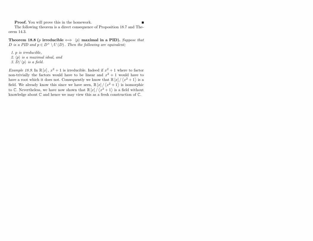
Proof. You will prove this in the homework.The following theorem is a direct consequence of Proposition 18.7 and The-

orem 14.3.

Theorem 18.8 (p irreducible ⇐⇒ 〈p〉 maximal in a PID). Suppose thatD is a PID and p ∈ D× \ U (D) . Then the following are equivalent;

1. p is irreducible,2. 〈p〉 is a maximal ideal, and3. D/ 〈p〉 is a field.

Example 18.9. In R [x] , x2 + 1 is irreducible. Indeed if x2 + 1 where to factornon-trivially the factors would have to be linear and x2 + 1 would have tohave a root which it does not. Consequently we know that R [x] /

⟨x2 + 1

⟩is a

field. We already know this since we have seen, R [x] /⟨x2 + 1

⟩is isomorphic

to C. Nevertheless, we have now shown that R [x] /⟨x2 + 1

⟩is a field without

knowledge about C and hence we may view this as a fresh construction of C.

19

Lecture 19

19.1 Irreducibles Polynomials I

Let F be a field – later it will be Q. Our goal is to determine when a polynomial,p (x) ∈ F [x] , is irreducible. We start with the following general results.

Example 19.1 (Second proof of Lemma 18.5). Let F be a field and λ ∈ F. Thenϕ : F [x]→ F be the evaluation homomorphism, ϕ (p) = p (λ) . Then ϕ (F [x]) =F, I = ker (ϕ) = 〈x− λ〉 = F [x] · (x− λ) , and therefore, F [x] / 〈x− λ〉 ∼= Fand therefore x− λ is irreducible in F [x] for all λ ∈ F by Theorem 18.8.

Lemma 19.2. If F is a field, f (x) ∈ F [x] with deg (f) ≥ 2, and f has a zeroin F , then f is reducible over F.

Proof. Let a ∈ F be a root of f, then f (x) = (x− a) k (x) for some k (x) ∈F (x) with deg (k) ≥ 1. Since both (x− a) and k (x) are not units, it followsthat f is reducible.

We have the following partial converse to this lemma.

Theorem 19.3. If F is a field, f (x) ∈ F [x] with deg (f) = 2 or deg (f) = 3,then f is irreducible over F iff f has no zeros in F.

Proof. Lemma 19.2 shows that f has zero implies f is reducible. Converselyif f is reducible, then f (x) = p (x) q (x) for some polynomials p and q withdeg (p) ,deg (q) ≥ 1. Since deg (p) + deg (q) = deg (f) ≤ 3, it follows thatdeg (p) = 1 or deg (q) = 1, say deg (p) = 1. Thus p (x) = ax + b for somea, b ∈ F with a 6= 0 and f (x) = (ax+ b) q (x) . Therefore

f

(−ba

)=(a−ba

+ b

)q

(−ba

)= 0 · q

(−ba

)which shows that f has a zero in F.

Example 19.4 (Construction of finite fields). Observe that the x3 function onZ5 is given by

x 0 1 2 3 4x3 0 1 3 2 4

.

Let f (x) := x3 + x+ 1 ∈ Z5 [x] , then

x 0 1 2 3 4f (x) 1 3 1 1 4

showing f (x) has not roots and hence is irreducible. Therefore 〈f (x)〉 ⊂ Z5 [x]is a maximal ideal and therefore,

F := Z5 [x] / 〈f (x)〉

is a field. As we have,

F ={[a+ bx+ cx2

]: a, b, c ∈ Z5

},

we see that the number of elements in F is 53 = 125. Thus we have constructeda field with 125 elements and characteristic 5.

Proposition 19.5. Suppose that f (x) =∑nk=0 akx

k ∈ Z [x] . If and f (r/s) = 0for some r ∈ Z and s ∈ Z+ with gcd (r, s) = 1, .then s|an and r|a0. In particularif f (x) is monic, i.e. an = 1, the only possible rational roots of f (x) mustactually be in Z and in fact must be a divisor of a0.

Proof. See problem 17.25 in Gallian which you are assigned for homework.

Example 19.6. Let k ≥ 2 and p be a prime in Z+, then k√p is irrational. Indeed

if k√p = r were rational, being a root of xk − p, r would have to be an integer

which divides p by Proposition 19.5. Thus r would have to be ±p or ±1 none ofwhich will work. Hence we may conclude that x2− p and x3− p are irreduciblepolynomials over Q (or Z) for any prime number p. (In fact by Eisenstein’sCriterion, Theorem 22.6 below, it is easy to see that xk − p is irreducible overQ for all primes, p, and k ≥ 2.) Of course

x2 − 2 =(x−√

2)(

x+√

2)

in R [x]

and therefore x2 − 2 is reducible over R.

Example 19.7. In this example we consider the polynomial, x2 + 1 ∈ F [x] for anumber of fields, F.

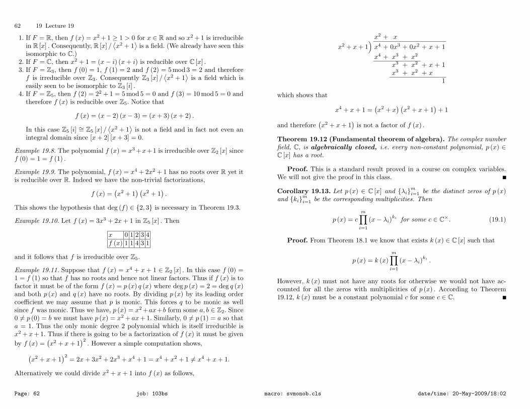
62 19 Lecture 19

1. If F = R, then f (x) = x2 + 1 ≥ 1 > 0 for x ∈ R and so x2 + 1 is irreduciblein R [x] . Consequently, R [x] /

⟨x2 + 1

⟩is a field. (We already have seen this

isomorphic to C.)2. If F = C, then x2 + 1 = (x− i) (x+ i) is reducible over C [x] .3. If F = Z3, then f (0) = 1, f (1) = 2 and f (2) = 5 mod 3 = 2 and thereforef is irreducible over Z3. Consequently Z3 [x] /

⟨x2 + 1

⟩is a field which is

easily seen to be isomorphic to Z3 [i] .4. If F = Z5, then f (2) = 22 + 1 = 5 mod 5 = 0 and f (3) = 10 mod 5 = 0 and

therefore f (x) is reducible over Z5. Notice that

f (x) = (x− 2) (x− 3) = (x+ 3) (x+ 2) .

In this case Z5 [i] ∼= Z5 [x] /⟨x2 + 1

⟩is not a field and in fact not even an

integral domain since [x+ 2] [x+ 3] = 0.

Example 19.8. The polynomial f (x) = x3 +x+1 is irreducible over Z2 [x] sincef (0) = 1 = f (1) .

Example 19.9. The polynomial, f (x) = x4 + 2x2 + 1 has no roots over R yet itis reducible over R. Indeed we have the non-trivial factorizations,

f (x) =(x2 + 1

) (x2 + 1

).

This shows the hypothesis that deg (f) ∈ {2, 3} is necessary in Theorem 19.3.

Example 19.10. Let f (x) = 3x3 + 2x+ 1 in Z5 [x] . Then

x 0 1 2 3 4f (x) 1 1 4 3 1

and it follows that f is irreducible over Z5.

Example 19.11. Suppose that f (x) = x4 + x + 1 ∈ Z2 [x] . In this case f (0) =1 = f (1) so that f has no roots and hence not linear factors. Thus if f (x) is tofactor it must be of the form f (x) = p (x) q (x) where deg p (x) = 2 = deg q (x)and both p (x) and q (x) have no roots. By dividing p (x) by its leading ordercoefficient we may assume that p is monic. This forces q to be monic as wellsince f was monic. Thus we have, p (x) = x2 +ax+b form some a, b ∈ Z2. Since0 6= p (0) = b we must have p (x) = x2 + ax+ 1. Similarly, 0 6= p (1) = a so thata = 1. Thus the only monic degree 2 polynomial which is itself irreducible isx2 + x+ 1. Thus if there is going to be a factorization of f (x) it must be givenby f (x) =

(x2 + x+ 1

)2. However a simple computation shows,(

x2 + x+ 1)2

= 2x+ 3x2 + 2x3 + x4 + 1 = x4 + x2 + 1 6= x4 + x+ 1.

Alternatively we could divide x2 + x+ 1 into f (x) as follows,

x2 + x

x2 + x+ 1)x4 + 0x3 + 0x2 + x + 1x4 + x3 + x2

x3 + x2 + x + 1x3 + x2 + x

1

which shows that

x4 + x+ 1 =(x2 + x

) (x2 + x+ 1

)+ 1

and therefore(x2 + x+ 1

)is not a factor of f (x) .

Theorem 19.12 (Fundamental theorem of algebra). The complex numberfield, C, is algebraically closed, i.e. every non-constant polynomial, p (x) ∈C [x] has a root.

Proof. This is a standard result proved in a course on complex variables.We will not give the proof in this class.

Corollary 19.13. Let p (x) ∈ C [x] and {λi}mi=1 be the distinct zeros of p (x)and {ki}mi=1 be the corresponding multiplicities. Then

p (x) = cm∏i=1

(x− λi)ki for some c ∈ C×. (19.1)

Proof. From Theorem 18.1 we know that exists k (x) ∈ C [x] such that

p (x) = k (x)m∏i=1

(x− λi)ki .

However, k (x) must not have any roots for otherwise we would not have ac-counted for all the zeros with multiplicities of p (x) . According to Theorem19.12, k (x) must be a constant polynomial c for some c ∈ C.


20

Lecture 20

Corollary 20.1. The only irreducible polynomials in C [x] are those with de-gree equal to one. The only irreducible polynomials in R [x] are the degree onepolynomials and the degree two polynomials with no roots.

Proof. The first assertion should be clear from Corollary 19.13. For thesecond assertion, suppose that p (x) ∈ R [x] is any polynomial. If λ ∈ C is aroot of p (x) , then 0 = p (λ) = p

(λ)

because p (x) has all real coefficients. Letus now suppose that p (x) is irreducible over R.

If λ ∈ R is a root of p (x) , then p (x) = (x− λ) k (x) for some k (x) ∈ R [x] .Since p (x) is irreducible we must have deg (k (x)) = 0, i.e. .k (x) is a constantand p (x) is linear. On the other hand if λ ∈ C \ R is a root of p (x) then so isλ. Therefore we know

p (x) = (x− λ)(x− λ

)k (x) =

(x2 − 2 Reλ+ |λ|2

)k (x)

for some k (x) ∈ R [x] . Since p (x) is irreducible, we must again have deg k (x) =2. This observation along with Theorem 19.3 completes the proof of the corol-lary.

Proposition 20.2. Let p (x) ∈ R [x] , then p (x) may be factored into irre-ducibles of R [x] .

Proof. If p (x) is not irreducible, there exists h (x) , k (x) ∈ R [x] withdeg h ≥ 1, deg k ≥ 1, and p (x) = h (x) k (x) . Since deg h (x) < deg p (x) and ddeg k (x) < deg p (x) , the result follows by a simple induction argument.

20.1 Two more homomorphisms involving polynomials

Lemma 20.3. Let R and T be commutative rings, ϕ : R [x] → T be a ringhomomorphism, and let t := ϕ (x) . Then

ϕ

(n∑k=0

akxk

)=

n∑k=0

ϕ (ak) tk for alln∑k=0

akxk ∈ R [x] .

Proof. Using the ring homomorphism properties we find,

ϕ (p (x)) =n∑k=0

ϕ(akx

k)

=n∑k=0

ϕ (ak)ϕ(xk)

=n∑k=0

ϕ (ak)ϕ (x)k =n∑k=0

ϕ (ak) tk.

Proposition 20.4 (Changing coefficients). Let R and T be commutativerings and ψ : R→ T be a ring homomorphism. Further define ψ : R [x]→ T [x]by the formula,

ψ

(n∑k=0

akxk

):=

n∑k=0

ψ (ak)xk for alln∑k=0

akxk ∈ R [x] . (20.1)

Then ψ is a ring homomorphism. Moreover this is the unique ring homo-morphism from R [x] → T [x] such that ψ (x) = x and ψ (a) = ψ (a) for alla ∈ R ⊂ R [x] .

Proof. You are asked to prove this for homework.

Example 20.5. Suppose that ψk : Z→ Zk is the homomorphism, ψk (a) :=amod k so that ψk : Z [x]→ Zk [x] . For example,

ψ3

(5x3 + 7x+ 3

)= 2x3 + x ∈ Z3 [x] ,

ψ5

(5x3 + 7x+ 3

)= 2x+ 3 ∈ Z5 [x] , and

ψ7

(5x3 + 7x+ 3

)= 5x3 + 3 ∈ Z7 [x] .

Corollary 20.6. Let R and T be commutative rings and ϕ : R → T be aring homomorphism. Then for each t ∈ T there exists a ring homomorphismϕt : R [x] → T such that ϕt (a) = ϕ (a) for all a ∈ R and ϕt (x) = t. Morespecifically, if

ϕt

(n∑k=0

akxk

)=

n∑k=0

ϕ (ak) tk for alln∑k=0

akxk ∈ R [x] .

64 20 Lecture 20

Proof. Let ψ : R [x]→ T [x] be the homomorphism in Proposition 20.4 andevt : T [x] → T be the evaluation homomorphism at t. Then ϕt = evt ◦ ψ :R [x]→ T is the desired homomorphism.

Example 20.7. As an application of Corollary 20.6, let R be a commutativering, ϕ : R → R [x] be the homomorphism taking a ∈ R to the constantpolynomial a ∈ R [x] , and t (x) ∈ R [x] be any polynomial. Then there is aunique homomorphism, ϕt : R [x] → R [x] such that ϕt (a) = a for all a ∈ Rand ϕt (x) = t (x) which is given formulaically as,

ϕ (p (x)) = p (t (x)) for all p (x) ∈ R [x] .

In particular if t (x) = x−a for some a ∈ R the map, p (x)→ p (x− a) is a ringisomorphism from R [x] to R [x] with inverse being given by p (x)→ p (x+ a) .

20.2 Gauss’ Lemma

We now go back to finding more ways to determine when f (x) ∈ Q [x] is irre-ducible. Are first goal is to change the question into one involving a polynomialg (x) ∈ Z [x] being irreducible or not – see Corollary 21.5 below. The main toolhere will be Gauss’ Lemma 20.10 below.

Definition 20.8. Let f (x) =∑nk=0 anx

n ∈ Z [x] , then c (f) := gcd (a0, . . . , an)is called the content of f. A polynomial f ∈ Z [x] is said to be primitive ifc (f) = 1.

Example 20.9. If f (x) = 14x2+10x+6, then c (f) = 2 and 12f (x) = 7x2+5x+3

is a primitive polynomial.

Lemma 20.10 (Gauss’ Lemma). If f (x) , g (x) ∈ Z [x] are primitive polyno-mials, then f (x) g (x) is primitive as well, i.e. c (f) = 1 = c (g) =⇒ c (fg) = 1.

Proof. Suppose that c (fg) > 1 and let p be a prime divisor of c (fg) .Further let f (x) :=

∑nk=0 (an mod p)xn and similarly for g (x) . Observe that

f → f is a ring homomorphism from Z [x] → Zp [x] so that fg = f g. Sincep divides all of the coefficients of fg we know fg = 0 and since Zp [x] is anintegral domain, we may conclude that either f = 0 or g = 0, i.e. p|c (f) orp|c (g) . Thus at least one of the polynomials, f or g, is not primitive.

Lemma 20.11. Suppose that a0, . . . , an ∈ Z (not all zero) and m ∈ Z+. Thengcd (ma0, . . . ,man) = m gcd (a0, . . . , an) . In particular if f (x) ∈ Z [x] andm ∈ Z×, then c (mf) = |m| c (f) .

Proof. First Proof. One way to compute the gcd of a bunch of numbersis by looking at their prime number decompositions. In terms of this decompo-sition,

gcd (a0, . . . , an) =N∏i=1

pkii

where {pi}Ni=1 are the distinct primes which appear in these decomposition andki ∈ {0, 1, 2, . . . } is chosen so that pki

i |aj for all j but pki+1i does not divide one

of the aj . Using this description it is easy to see the truth of the lemma.Second Proof. Let d := gcd (a0, . . . , an) and c := gcd (ma0, . . . ,man) then

we know there exists si ∈ Z such that

d = s0a0 + · · ·+ snan.

From this it follows that

md = s0ma0 + · · ·+ snman.

Thus every common divisor of mai for all i is a divisor of md and in particularc| (md) . Since md is a divisor of mai for all i we also know that md|c. Thus wemay conclude that md = c as claimed.

Corollary 20.12. If f, g ∈ Z [x] then c (fg) = c (f) · c (g) . In particular,f (x) g (x) is primitive iff both f (x) and g (x) are primitive.

Proof. Let f0 (x) := 1c(f)f (x) and g0 (x) := 1

c(g)g (x) so that both f0 (x) andg0 (x) are primitive in Z [x] . Then by Gauss’ lemma, f0 (x) g0 (x) is primitiveand since f (x) g (x) = c (f) c (g) f0 (x) g0 (x) , it follows from Lemma 20.11 thatc (fg) = c (f) c (g) .

Corollary 20.13. Suppose that f (x) , g (x) ∈ Z [x] , g (x) is primitive, andk (x) ∈ Q [x] . If f (x) = k (x) g (x) in Q [x] , then k (x) ∈ Z [x] . In words ifg (x) divides f (x) in Q [x] then the quotient is in fact back in Z [x] .

Proof. Let t ∈ Z+ be chosen so that h (x) := tk (x) ∈ Z [x] – for examplelet t be the least common multiple of all of the denominators in the coefficientsof k (x) . We then have tf (x) = h (x) g (x) therefore that tc (f) = c (tf) =c (h) c (g) = c (h) . It now follows that

1c (f)

f (x) =1

c (tf)tf (x) =

1c (h)

tf (x) =1

c (h)h (x) g (x) =

1c (h)

h (x) g (x) .

Thereforef (x) = c (f)

1c (h)

h (x) g (x) = k (x) g (x)


and hence

k (x) = c (f)(

1c (h)

h (x))∈ Z [x] .

Example 20.14. If g (x) is not primitive, the results in Corollary 20.13 may fail.For example take f (x) = x2, g (x) = 2x and k (x) = 1

2x.

21

Lecture 21

Lemma 21.1. Suppose that f (x) , g (x) ∈ Z [x] are primitive polynomials andthere exists α, β ∈ Q× such that αf (x) = βg (x) as polynomials in Q [x] . Then|α| = |β| and f (x) = ±g (x) .

Proof. Apply Corollary 20.13 with k (x) = β/α to learn that β/α = t ∈ Z.Since f (x) = tg (x) it follows that 1 = c (f) = |t| c (g) = |t| so that β/α = t =±1.

Alternative Proof. Let α := ab and β := u

v with a, b, u, v ∈ Z\ {0} . Thenvaf (x) = ubg (x) . From Lemma 20.11 we know

|va| = c (vaf (x)) = c (ubg (x)) = |ub|

from which it follows that f (x) = ±g (x) .

Example 21.2. The polynomial, f (x) = x2 − 5x + 6 ∈ Z [x] has a factorizationover Q as

f (x) =(

12x− 3

2

)(2x− 4) .

Of course if we move the factor of 2 from the second factor to the first we alsohave the factorizations of f (x) over Z as,

f (x) = (x− 3) (x− 2) .

The next theorem shows this sort of rejiggering can always be done.

Theorem 21.3. Let f (x) ∈ Z [x] . If f (x) is reducible over Q then f (x) isreducible over Z. In fact f (x) is reducible over Q [x] iff f (x) factors in Z [x] inthe form, f (x) = u (x) v (x), where u (x) , v (x) ∈ Z [x] with deg u (x) ≥ 1 anddeg v (x) ≥ 1.

Consequently: if f (x) is irreducible over Z then f (x) is also irreducibleover Q.

Proof. We need to show that any non-trivial factorization over Q gives riseto a non-trivial factorization over Z. So suppose f (x) ∈ Z [x] and h (x) , g (x) ∈Q [x] with deg (h) ≥ 1, deg (g) ≥ 1, and f (x) = g (x)h (x) in Q [x] . Chooses, t ∈ Z+ such that g1 (x) := sg (x) and h1 (x) := th (x) and in Z [x] . Then wehave

stf (x) = g1 (x)h1 (x) =⇒ stc (f) = c (g1) · c (h1)

and therefore

1c (f)

f (x) =1

stc (f)stf (x) =

1c (g1)

g1 (x) · 1c (h1)

h1 (x) .

Therefore we have found a non-trivial factorization of f (x) over Z in the desiredform, namely;

f (x) =[c (f)

1c (g1)

g1 (x)]·[

1c (h1)

h1 (x)]

=[c (f)

s

c (g1)g (x)

]·[

t

c (h1)h (x)

]=: u (x) v (x) .

Example 21.4. Notice that x ∈ Z [x] is irreducible. Indeed if x = f (x) g (x) forsome f (x) , g (x) ∈ Z [x] , then 1 = deg (f (x))+deg (g (x)) and we may supposethat deg (f) = 1 and deg (g) = 0. Moreover we know that f (x) and g (x) areprimitive and therefore g (x) = ±1 ∈ U (Z [x]) . Thus the factorization is trivialand x ∈ Z [x] is irreducible.

On the other hand, f (x) = 5x ∈ Z [x] is reducible over Z but irreducibleover Q. The point being that 5 ∈ U (Q) while 5 /∈ U (Z) .

However we do have the following corollary to Theorem 21.3.

Corollary 21.5. If f (x) ∈ Z [x] is primitive, then f (x) is irreducible overZ [x] iff f (x) is irreducible over Q [x] .

Proof. 1. First observe that if g (x) /∈ U (Z [x]) and g (x) is primitive thendeg g (x) ≥ 1. Indeed if deg g (x) = 0 and g (x) is primitive, then g (x) = ±1,i.e. g (x) ∈ U (Z [x]) .

2. Suppose that f (x) is primitive and reducible over Z, i.e. f (x) = g (x)h (x)for some g (x) , h (x) /∈ U (Z [x]) . Since 1 = c (f) = c (g) c (h) it follows thatc (g) = 1 = c (h) and therefore by the first part we must have deg g (x) ≥ 1 anddeg h (x) ≥ 1. Therefore g (x) , h (x) /∈ U (Q [x]) ∼= Q× and so the factorizationf (x) = g (x)h (x) is nontrivial over Q as well, i.e. f (x) is reducible in Q [x] .Since the converse was already proven in Theorem 21.3, the proof is complete.

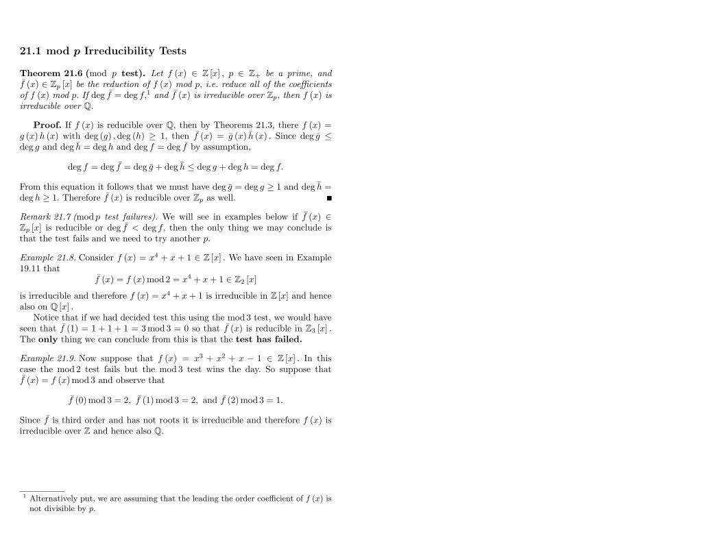
21.1 mod p Irreducibility Tests

Theorem 21.6 (mod p test). Let f (x) ∈ Z [x] , p ∈ Z+ be a prime, andf (x) ∈ Zp [x] be the reduction of f (x) mod p, i.e. reduce all of the coefficientsof f (x) mod p. If deg f = deg f,1 and f (x) is irreducible over Zp, then f (x) isirreducible over Q.

Proof. If f (x) is reducible over Q, then by Theorems 21.3, there f (x) =g (x)h (x) with deg (g) ,deg (h) ≥ 1, then f (x) = g (x) h (x) . Since deg g ≤deg g and deg h = deg h and deg f = deg f by assumption,

deg f = deg f = deg g + deg h ≤ deg g + deg h = deg f.

From this equation it follows that we must have deg g = deg g ≥ 1 and deg h =deg h ≥ 1. Therefore f (x) is reducible over Zp as well.

Remark 21.7 (mod p test failures). We will see in examples below if f (x) ∈Zp [x] is reducible or deg f < deg f, then the only thing we may conclude isthat the test fails and we need to try another p.

Example 21.8. Consider f (x) = x4 + x + 1 ∈ Z [x] . We have seen in Example19.11 that

f (x) = f (x) mod 2 = x4 + x+ 1 ∈ Z2 [x]

is irreducible and therefore f (x) = x4 + x+ 1 is irreducible in Z [x] and hencealso on Q [x] .

Notice that if we had decided test this using the mod 3 test, we would haveseen that f (1) = 1 + 1 + 1 = 3 mod 3 = 0 so that f (x) is reducible in Z3 [x] .The only thing we can conclude from this is that the test has failed.

Example 21.9. Now suppose that f (x) = x3 + x2 + x − 1 ∈ Z [x] . In thiscase the mod 2 test fails but the mod 3 test wins the day. So suppose thatf (x) = f (x) mod 3 and observe that

f (0) mod 3 = 2, f (1) mod 3 = 2, and f (2) mod 3 = 1.

Since f is third order and has not roots it is irreducible and therefore f (x) isirreducible over Z and hence also Q.

1 Alternatively put, we are assuming that the leading the order coefficient of f (x) isnot divisible by p.

22

Lecture 22

Let f (x) ∈ Z [x] and for any prime p ≥ 2, let fp (x) := f (x) mod p. Thencombining Theorems 21.3 and 21.6 we have the following implication; ∃ p such that

deg fp (x) = deg f (x) &fp (x) ∈ Zp [x] is irreducible

=⇒(f (x) is irreducible

over Q

).

Example 22.1. Let us consider the polynomial,

f (x) := 5x4 − 83x3 + 3x+

113∈ Q [x] .

Then f (x) is irreducible iff

g (x) := 3f (x) = 15x4 − 8x3 + 9x+ 11

is irreducible over Q. As g (x) ∈ Z [x] and c (g) = 1 we need only show thatg (x) is irreducible over Z [x] . To test this out, let g (x) be g (x) mod 2, so that

g (x) = x4 + x+ 1 ∈ Z2 [x] .

We have already seen in Example 19.11 that g (x) is irreducible and thereforeby the mod 2 test, g (x) is irreducible and therefore so is 3f (x) ∈ Z [x] andhence f (x) ∈ Q [x] .

Example 22.2 (Converse of mod p test is false). Let f (x) := x2+5x+25 ∈ Z [x]and f (x) = x2 be f (x) mod 5. Notice that f is reducible over Z5 yet f (x) isirreducible over Q. Indeed, it is easy to see that f (x) has not roots in Z andhence not roots in Q. Alternatively, apply the mod 2 test in which case weconsider x2 +x+1 which is irreducible over Z2 as it has no roots. Alternatively,by the quadratic formula the roots of f (x) are given by

−5±√

25− 1002

=−5± i

√75

2so there are not even any real roots. This can also be seen by completing thesquares to see,

f (x) =(x+

52

)2

+ 25−(

52

)2

=(x+

52

)2

+ 25 · 34≥ 75

4.

Example 22.3 (Degree hypothesis is necessary). Let

f (x) = 2x2 + 3x+ 1 = (2x+ 1) (x+ 1) ∈ Q [x] . (22.1)

Clearly this polynomial is reducible. On the on the other hand if we reduce fmod 2 we get the polynomial, f (x) = x+1 which is linear and hence irreducible.Notice that under the mod 2 reduction, the factorization in Eq. (22.1) becomes,

x+ 1 = 1 · (x+ 1)

which is a trivial factorization of x+ 1.

Example 22.4. Let us determine if

f (x) :=37x3 +

57x+

17∈ Q [x]

is irreducible or not. We need only consider 7f (x) = 3x3 + 5x + 1 which isprimitive in Z [x].

Plot of 7f (x) .

Let us consider

g (x) := 7f (x) mod 2 = x3 + x+ 1.

Since g (0) = g (1) = 1, it follows that g is irreducible and since deg (g) =deg (7f) , we learn that 7f and hence f is irreducible over Q.

Alternatively we may use Proposition 19.5 to argue that 7f (x) and hencef (x) has no roots in Q. According to Proposition 19.5 we need only look for

70 22 Lecture 22

roots of the form a/3 where a ∈ {±1} that is we need only consider {0,±1/3} .By direct calculation we learn

7f (−1/3) = −7/9 6= 0 and 7f (1/3) =2596= 0.

This again shows that f (x) is irreducible over Q [x] .

Example 22.5. Let us show again the f (x) = x3 + 5 is irreducible over Q.

1. Method 1. By Proposition 19.5 the only possible roots of f (x) are for x ∈{±5} and it is clear that neither of these are roots of f (x) .

2. Method 2. Let us try the mod p tests.a) For p = 2 and p = 3 the tests fails since 1 is a root in each of these

cases.b) For p = 5, f (x) = x3 is clearly reducible so the test fails again.c) For p = 7 we find

f (0) mod 7 = 5, f (1) mod 7 = 6, f (2) mod 7 = 6, f (3) mod 7 = 4,f (4) mod 7 = 6, f (5) mod 7 = 4, f (6) mod 7 = 4

and the test has succeeded in showing that x3 + 5 is irreducible over Q.3. Method 3. Use Eisenstein’s criteria in Theorem 22.6 below.

22.1 Eisenstein’s Criterion

Theorem 22.6 (Eisenstein’s Criterion). Let f (x) :=∑nk=0 akx

k ∈ Z [x]with n ≥ 2. If there is a prime p such that p - an, p2 - a0 while p|aj forj = 0, 1, 2, . . . , n− 1 then f (x) is irreducible. over Q.

Proof. If f (x) were reducible over Q [x] then, by Theorem 21.3, there existsg (x) , h (x) ∈ Z [x] with deg (g) ,deg (h) ≥ 1 such that f (x) = g (x)h (x) . Let

g (x) =r∑

k=0

gkxk and h (x) =

s∑k=0

hkxk

where r + s = n.In order to absorb the general proof better let us first suppose that r = s = 1

so that

f (x) = (g0 + g1x) (h0 + h1x) = g0h0 + (g0h1 + g1h0)x+ g1h1x2.

Since p| (g0h0) and p2 - (g0h0) , we may assume that p|g0 but p - h0. Combiningthis with the assumption that p| (g0h1 + g1h0) implies that p|g1. But this then

implies p| (g1h1) which contradicts the assumption that p does not divide theleading order coefficient of f (x) .

With this as a warm-up we go to the general case. Notice that a0 = g0h0

and an = grhs. Since p|a0 while p2 - a0 it follows that p divides exactly one ofg0 or h0 but not both. Suppose that p|g0 and p - h0. Also notice that p - animplies p - gr so there is a first 0 < t ≤ r < n such that p - gt. Since,

at = g0ht + g1ht−1 + · · ·+ gt−1h1 + gth0,

and p|at, it follows that p|gth0 which then implies p|h0 which is a contradiction.

For a second proof of this theorem, see Theorem 24.7 below.

Example 22.7. The polynomial, x5+9x4+12x2+6 is irreducible over Q [x] sincep = 3 divides all of the coefficients except the leading order one and 32 - 6.

For n ∈ N, letΦn (x) = 1 + x+ x2 + · · ·+ xn−1.

This geometric series may be summed in the usual way,

xΦn (x)− Φn (x) = xn − 1 =⇒ Φn (x) =xn − 1x− 1

.

Corollary 22.8. For any prime, p ∈ N, Φp (x) is irreducible over Q.

Proof. Observe that

(x+ 1)p − 1 =p∑k=0

(p

k

)xk − 1 =

p∑k=1

(p

k

)xk,

(x+ 1)− 1 = x, and hence

Φp (x+ 1) =(x+ 1)p − 1(x+ 1)− 1

=∑pk=1

(pk

)xk

x=

p∑k=1

(p

k

)xk−1

= xp−1 +(

p

p− 1

)xp−2 +

(p

p− 2

)xp−3 + . . .

(p

2

)x+

(p

1

).

For 1 ≤ k < p, since there is no factor of p in k! or (p− k)!, it follows that(p

p− k

)=

p (p− 1)!k! (p− k)!

= p · (p− 1)!k! (p− k)!

is an integer which is divisible by p. Thus p|(p

p−k)

for 1 ≤ k ≤ p − 1 whilep2 -

(p1

)= p and hence the Eisenstein’s Criterion, Φp (x+ 1) is irreducible. This

then is easily seen to imply Φp (x) is irreducible.


22.2 Summary of irreducibility tests

Theorem 22.9 (Reducibility tests). Let F be a field and f (x) ∈ F [x] . Ifdeg f (x) = 1, then f (x) is irreducible so suppose that deg f (x) ≥ 2. Then;

(f (x) has a root

in F

)=⇒

(f (x) is reducible

over F

).

Moreover if deg f (x) = 2 or deg f (x) = 3, then(f (x) has a root

in F

)⇐⇒

(f (x) is reducible

over F

).

Theorem 22.10 (Finding roots). Suppose that f (x) =∑nk=0 akx

k ∈ Z [x]with an 6= 0 6= a0. Then the rational roots of f (x) are contained in{r

s: r ∈ N, s ∈ Z+ 3 s|an and r|a0

}.

Theorem 22.11 (Q – Irreducibility tests). Suppose f (x) =∑nk=0 akx

k ∈Z [x] with n := deg f (x) ≥ 2. Then;

deg f (x) = 1 ordeg f (x) = 2 or 3

& f (x) has noroots in Q

mod p test ⇓ Eisenstein’s

Criterion∃ a prime p 3

deg fp (x) = deg f (x)& fp (x) is irreducible

over Zp

=⇒(f (x) is irreducible

over Q

)⇐=

∃ a prime p

such thatp|ak for k < np - an & p2 - a0

.

⇑(f (x) is irreducible

over Z

)Moreover if f (x) is primitive (i.e. c (f) = 1) then(

f (x) is irreducibleover Q

)⇐⇒

(f (x) is irreducible

over Z

).

23

Lecture 23

23.1 Irreducibles and Primes II

Definition 23.1. Let D be an integral domain (i.e. a commutative ring with 1which has no zero divisors, i.e. cancellation holds in D) and a, b, c ∈ D. Then;

1. a is associated to b if a = b (mod)U (R) , i.e. a ∈ bU (R) or equivalentlyb ∈ aU (R) .

2. a ∈ D is irreducible iff a 6= 0, a /∈ U (R) and whenever a = bc then eitherb ∈ U (R) or c ∈ U (R) . (So a ∈ D is irreducible if it can not be factored ina non-trivial way.) Similarly we say that 0 6= a ∈ D is reducible if it admitsa factorization of the form a = bc with b, c /∈ U (R) .

3. a ∈ D is prime if 0 6= a /∈ U (R) and if a satisfies; whenever a|bc theneither a|b or a|c. (So a ∈ D is prime if the conclusion of Euclid’s lemmaholds.)

Example 23.2. Let R = Z so that U (Z) = {±1} and the associates to m are{±m} . Now 0 6= a ∈ Z is irreducible iff whenever a = bc we must have b or cis ±1. (That is |a| is prime in our old sense of the word.) It therefore followsby Euclid’s lemma (also see Theorem 23.6)) that if a|bc then a|b or a|c whichmeans that a is prime in our new sense of being prime as well. As will see inTheorem 23.4 below, prime always implies irreducible. Thus we are new notionof prime gives {±2,±3,±5,±7, . . . } for the primes in Z.

Proposition 23.3 (〈prime〉 is prime). Let D be an integral domain and a ∈D with 0 6= a /∈ U (R) . Then the following are equivalent;

1. a is prime.2. 〈a〉 = Ra is a prime ideal in D.3. R/ 〈a〉 is an integral domain.

Proof. See the homework.

Theorem 23.4 (Prime =⇒ irreducible). If D is an integral domain anda ∈ D is prime then a is irreducible.

Proof. Suppose that a ∈ D is a prime. If a = bc then a|b or a|c. Say thata|b, i.e. b = at. Then a = atc and since D is a domain we may cancel a form thisequation to see that 1 = tc. This shows that c ∈ U (R) and so a only admitstrivial factorizations, i.e. a is irreducible.

Theorem 23.5. Let R be an integral domain and 〈a〉 = Ra where a ∈ R witha 6= 0 and a /∈ U (R) . Then;

〈a〉 is maximal ideal ⇐⇒ R/ 〈a〉 is a field⇓ (1)

〈a〉 is a prime ideal ⇐⇒ R/ 〈a〉 is an integral domainm (2)

a is a prime element in R

⇓ (3)a is an irreducible element in R.

If we further assume that R is a PID, then the converse of all of the aboveimplications hold.1

Proof. The horizontal equivalences are contained in Theorem 14.3. The ver-tical implication (1) has been explained in Corollary 14.4. The vertical equiva-lence (2) is Proposition 23.3 and (3) is Theorem 23.4.

If R is now a PID, we know from Theorem 18.8 that a is irreducible implies〈a〉 is maximal. Therefore all statements in the theorem are now equivalent.

Remark 23.6 (Prime ⇐⇒ irreducible in a PID). Here is an alternative proofthat if D is a PID (principle ideal domain) and a ∈ D is irreducible then a isprime. Suppose that a ∈ D is irreducible and a|bc for some b, c ∈ D. Let

I := aD + bD := {ax+ by : x, y ∈ D} .

Notice that I is an ideal of D and hence I = 〈d〉 for some d ∈ D. Since a ∈ I wehave a = dr for some r ∈ D. As a is irreducible, either d ∈ U (R) or a ∈ U (R) .If d ∈ U (R) , then I = 〈d〉 = R and in particular 1 ∈ I. Thus there existsx, y ∈ D such that ax+ by = 1. Therefore,

axc+ ybc = c

from which it follows that a|c. On the other hand of r ∈ U (R) , then I = 〈d〉 =〈a〉 . Since b ∈ I it follows that b = at for some t ∈ D, i.e. a|b. So we have shownthat a|bc implies a|b or a|c, i.e. a is prime.1 More succinctly, if R is a PID and a ∈ R× \ U (R) is irreducible, then 〈a〉 is a

maximal ideal in R.

74 23 Lecture 23

Example 23.7. We have x ∈ Z [x] is prime and hence irreducible. Neverthe-less, 〈x〉 is not a maximal ideal as we have seen above. For example, 〈x〉 ${p (x) : p (0) is even} $ Z [x] . Thus we can not drop the assumption that D isa PID in Theorem 23.4. Nevertheless, we will see below in Theorem 24.1 thatf (x) ∈ Z [x] is prime iff it is irreducible in Z [x] .

Let me summarize the main theorems we have involving maximal and primeprinciple ideals and prime and irreducible elements of an integral domain R.

Example 23.8. In Z5, x2 + 1 has two zeros, namely x = 2 and x = 3. There-

fore, x2 + 1 factors as (x− 2) (x− 3) from which it follows that⟨x2 + 1

⟩is not a maximal ( ⇐⇒ prime) ideal in Z5 [x] . Therefore it follows thatZ5 [x] /

⟨x2 + 1

⟩ ∼= Z5 [i] is not a field and not even an integral domain. Ex-plicitly we have (i− 2) (i− 3) = 6− 1− 5i = 0 in Z5 [i] .

Remark 23.9. On the other hand, it is easy to verify that x2 + 1 has no zerosover Z3 and therefore x2 + 1 is irreducible over Z3. From this we may concludethat Z3 [i] ∼= Z3 [x] /

⟨x2 + 1

⟩is a field. This was already proved with some

effort in Example 5.3.

The next example shows that the converse of Theorem 23.4 is false in general.

Example 23.10 (Example 1, p. 321). In this example we will show that

α := 1 +√−3 ∈ R := Z

[√−3]

is irreducible but not prime which we will now verify. First observe that R isa sub-ring of C which will simplify our computations. Given x = a+b

√−3 ∈ R,

let x := a − b√−3 and N (x) := |x|2 = xx = a2 + 3b2 ∈ N. Since |xy| = |x| |y|

for all x, y ∈ C A direct calculation shows2 that N (xy) = N (x)N (y) for allx, y ∈ R.

• U (R) = {±1} . If xy = 1, then 1 = N (1) = N (x)N (y) implies N (x) =1 = N (y) . Conversely if N (x) = 1, then x−1 = x and therefore

U (R) = {x ∈ R : N (x) = 1} = {±1} .

• α is irreducible. If α = xy with x, y ∈ R, then 4 = N (α) = N (x)N (y) . Ifneither x nor y is a unit, we must have N (x) = 2 = N (y) which is impossiblesince N (x) = a2 + 3b2 which is never 2. Thus no such decomposition existsand α is irreducible.

2 You should check this by direct calculation if this is not familiar to you.

• α is not prime. Since αα = N (α) = 4, α|4 while 4 = 2 · 2. So if α wereprime we would have α|2, i.e. 2 = αx for some x = a + b

√−3. However if

2 = αx then 2α = α · αx = N (α)x = 4x. Thus we must have 2x = α, i.e.

2a+ 2b√−3 = 1−

√−3

which is impossible to do unless we take a = 1/2 and b = −1/2 neither ofwhich are in R. Thus we have shown α does not divide 2 and so α is notprime.

If time permits we will consider some other interesting integral domainswhich are not PID’s and for which some of the equivalences in Theorem 23.5no longer hold.


24

Lecture 24

It is possible for all irreducibles to be prime even if the ring is not a PID asthe next theorem shows.

Theorem 24.1 (Irreducible ⇐⇒ prime in Z[x]). If f (x) ∈ Z [x] is irre-ducible then f (x) is prime in Z [x] .

Proof. In the proof to follow we suppose that g (x) , h (x) ∈ Z [x] and thatf (x) |g (x)h (x) , i.e. there exists k (x) ∈ Z [x] such that

g (x)h (x) = k (x) f (x) . (24.1)

Case 1. Suppose that deg (f) = 0, i.e. f (x) is constant. Since f (x) is irre-ducible we must have f (x) = p where p is a prime in Z which we assume to bepositive for simplicity. Applying the content function, c (·) , to Eq. (24.1) gives

c (g) c (h) = c (k) c (f) = c (k) · p.

Therefore p|c (g) c (h) which implies p|c (g) or p|c (h) , i.e. p|g (x) or p|h (x) .Case 2. Suppose that deg (f) ≥ 1. In this case c (f) = 1 for otherwise

f (x) = c (f)[

1c (f)

f (x)]

would be a non-trivial factorization of f (x) over Z [x] . Since f (x) is primitiveand irreducible over Z [x] it is irreducible over Q [x] by Corollary 21.5. Thereforef (x) is prime in Q [x] and it follows that f (x) |g (x) or f (x) |h (x) in Q [x] . Butby Corollary 20.13 this implies that f (x) |g (x) or f (x) |h (x) in Z [x] , i.e. f (x)is prime in Z [x] .

24.1 Unique Factorization Domains

Definition 24.2 (UFD). A unique factorization domain (UFD for short)is an integral domain, R, such that

1. Every non-zero element of R which is not a unit may be written as a productof irreducibles in R.

2. The factorization into irreducibles is unique up to associates and the orderin which the factors appear. To be more precise, if a1, . . . , an and b1, . . . , bmare irreducibles in R such that a1 . . . an = b1 . . . bm then m = n and thereexists a permutation, σ ∈ Sn, such that ai and bσ(i) are associates for eachi.

Example 24.3. The fundamental theorem of arithmetic asserts that Z is a uniquefactorization domain.

Example 24.4 (Z[√−3] is not a UFD). Example 23.10 easily allows us to see

that R := Z[√−3]⊂ C is not a unique factorization domain. (see Definition

24.2 below). We have see that 4 ∈ R may be factored as 4 = 2 · 2 and also as4 = α · α where

α := 1 +√−3 and α := 1−

√−3.

Since the units of R are {±1} it is clear neither α nor α is associated to 2. (SeeChapter 18 of the book and in particular the comments on p. 333 as to whenZ[√

d]

is a UFD.)

Proposition 24.5. Suppose that R is a commutative ring with 1 ∈ R. If ai, bj ∈R are all elements of R which are prime and

a1 . . . am = b1 . . . bn,

then m = n and after a possible reordering of the {bi}ni=1 , we have ai and biare associates for each i.

Proof. We will give the proof using induction on N := max (m,n). For sakeof definiteness we assume that n = N. If N = 1, we have a1 = b1 and there isnothing to prove. For N = 2 we have either a1 = b1b2 or a1a2 = b1b2. In eithercase a1 being prime either divides b1 or b2. Relabeling the b’s if necessary, wemay assume that a1|b1, i.e. b1 = a1u1 for some u1 ∈ R. Since b1 is irreducibleand a1 /∈ U (R) we must have u1 ∈ U (R) so that a1 and b1 are associates.Thus we now have (using cancellation) that either 1 = u1b2 or a2 = u2b2. Thefirst case implies b2 ∈ U (R) which contradicts b2 being irreducible so it can notoccur. In the second case a2 and b2 are associates.

With this as warm up let us now do the general induction argument. Supposethat N = max (m,n) = n ≥ 2 and the result hold for lower N. Then working

76 24 Lecture 24

as above, after relabeling the b’s is necessary we may assume that b1 = a1u1 forsome u1 ∈ U (R) . If m = 1, this would imply that 1 = b2 . . . bn showing that allthe remaining bi are units which is impossible. Therefore we must have m ≥ 2and we now have (

u−11 a2

). . . am = b2b3 . . . bn = b′2 . . . b

′n.

By the induction hypothesis we now may conclude that m = n and that afterrelabeling the {bi} that

u−11 a2 = u2b2, a3 = u3b3, . . . , an = unbn

for some ui ∈ U (R) . This completes the proof since a2 = u1u2b2 and u1u2 ∈U (R) .

Because of this proposition we see that the uniqueness of factorizations intoirreducibles will hold if we can show the irreducibles are prime. In general weknow that primes are irreducibles, however it is not always true that irreduciblesare primes – see Example 32.2 below.

Theorem 24.6 (F [x] is a UFD). If F is a field, then F [x] is a unique fac-torization domain.

Proof. Let f (x) ∈ F [x] with deg (f) ≥ 1. If f (x) is not irreducible, thenf (x) = g (x)h (x) for some g (x) , h (x) ∈ F [x] with deg g ≥ 1 and deg h ≥ 1.Since deg g + deg h = deg f we must have deg g < deg f and deg h < deg f.By further decomposing g (x) and h (x) is possible we must eventually arriveat a decomposition of f (x) into irreducibles which gives the desired existence.(You may add the formal the induction proof if you wish.) The uniqueness ofthis factorization follows from Proposition 24.5 and the fact that primes andirreducibles are the same in a PID like F [x] , see Theorem 23.6.

As an application of this theorem let us give another proof of Eisenstein’sCriterion – see Theorem 22.6. For the readers convenience we repeat the state-ment here.

Theorem 24.7 (Eisenstein’s Criterion). Let f (x) :=∑nk=0 akx

k ∈ Z [x] .If there is a prime p such that p - an, p2 - a0 while p|aj for j = 0, 1, 2, . . . , n− 1then f (x) is irreducible. over Q.

Proof. If f (x) were reducible over Q [x] then, by Theorem 21.3, it wouldbe reducible over Z [x] and in fact there would exists g (x) , h (x) ∈ Z [x] withdeg (g) ,deg (h) ≥ 1 such that f (x) = g (x)h (x) . Letting f , g and h be thereductions of f, g, and h mod p we find, anxn = g (x) h (x) wherein we have usean := an mod p 6= 0 in Zp. Since Zp is a field, Zp [x] is a UFD and because deg gand deg h are both less than n we must have x divides both g (x) and h (x) . (Infact there must exist b, c ∈ Z×p such that g (x) = bxdeg g and h (x) = cxdeg h.)This then implies that p|g (0) and p|h (0) and therefore p2|a0 as a0 = g (0)h (0) .However this contradicts the assumption that p2 - a0.

Theorem 24.8 (Z[x] is a UFD). Z [x] is a unique factorization domain.

Proof. Existence. Let f (x) ∈ Z [x] and set f0 (x) := 1c(f)f0 (x) so that

f (x) = c (f) f0 (x) where f0 (x) is primitive. Since we may factor c (f) intoprime integers which are irreducible in Z [x] it suffices to factor f0 (x) intoirreducibles. So from now on we assume that f (x) is primitive.

If f (x) is not irreducible, the f (x) = h (x) g (x) with neither h (x) or g (x)being invertible. Since c (h) c (g) = c (f) = 1 we know that both h and g areprimitive and therefore deg h ≥ 1 and deg g ≥ 1. Since deg f = deg h+deg g, wemust have deg h < deg f and deg g < deg f. Thus the existence of a factorizationof f (x) when f (x) is primitive goes just as in the proof of Theorem 24.6.

Uniqueness. The uniqueness of the factorization follows by combiningProposition 24.5 with Theorem 24.1.

Fact 24.9 (Facts about UFD’s) Here are two more facts about unique fac-torization domains which we will not prove in class.

1. Every PID is a UFD. This is proved in Gallian and is fairly similar to theproof of Theorem 24.6.

2. If R a UFD then R [x] is a UFD. Our proof that Z [x] is a UFD is rathersimilar to the general case – see Knapp [1, pgs. 384-396] for details.


25

Extra Topics (Not covered in class)

25.1 Greatest Common Divisors

Definition 25.1. Let R be an integral domain. We say that c ∈ R is a commondivisor of a1, . . . , an ∈ R if c|ai for all i. We say that d ∈ R is a greatestcommon divisor of a1, . . . , an ∈ R if d is a divisor and if c|d for any otherdivisor of a1, . . . , an ∈ R.

If c and d are two greatest common divisors of a1, . . . , an ∈ R, then c = udand d = vc for some u, v ∈ R. Therefore, c = uvc and since R is an integraldomain, uv = 1 by cancellation. Thus c and d are associates and the gcd ofa1, . . . , an is well defined modulo U (R) .

Proposition 25.2. If R is a PID, then every list of elements, a1, . . . , an ∈ R×,has a greatest common divisor, d. Moreover there exists r1, . . . , rn ∈ R suchthat

d = r1a1 + · · ·+ riai + · · ·+ rnan. (25.1)

Proof. Let J = 〈a1, . . . , an〉 = 〈a1〉+ · · ·+ 〈an〉 be the ideal of R generatedby (a1, . . . , an) and choose c ∈ R such that J = 〈c〉 . Then by definition of J,c may be expressed as in Eq. (25.1) and ai ∈ 〈c〉 for all i. The latter conditionasserts that c|ai for all i so that c is a common divisor and it follows from Eq.(25.1) that in fact c is a greatest common divisor.

Definition 25.3. As in the case R = Z we will say that elements, a1, . . . , anin a PID, R, are relatively prime if the greatest common divisors are units.Alternatively, this is equivalent to saying 1 ∈ gcd (a1, . . . , an) .

Here is the analogue of Euclid’s Lemma in this more general context.

Lemma 25.4 (Euclid’s Lemma II). Let R be a PID and a, b, c ∈ R with a, bbeing relatively prime. If a| (bc) then a|c.

Proof. From Proposition 25.2 we know that 1 = sa+ tb for some s, t ∈ R.Therefore c = sac+ tbc from which it follows that a|c.

Remark 25.5. If F is a field and p (x) , q (x) ∈ F [x] are two non-zero polynomi-als, one may find gcd (p, q) using the division algorithm just as we did for theintegers, Z. The point is to repeatedly make use of the fact that

gcd (p, q) = gcd (q, qmod p)

where qmod p denotes the remainder from dividing p into q.where qmod p de-notes the remainder from dividing p into q.

The next result has already been proved in Theorem 18.8. Nevertheless it isinstructive to give another proof.

Corollary 25.6. Suppose that F is a field and p (x) ∈ F [x] is irreducible. ThenF [x] / 〈p (x)〉 is a field.

Proof. If f (x) ∈ F [x] with deg f (x) < deg p (x) , then f (x) and p (x) arerelatively prime since the only possible non-trivial common factor would bep (x) which is impossible since deg f (x) < deg p (x) . Therefore by Proposition25.2, there exists s (x) , t (x) ∈ F [x] such that

s (x) f (x) + t (x) p (x) = 1.

Since [p (x)] = 0 it follows that [s (x)] [f (x)] = 1 and we have shown [f (x)]−1 =[s (x)] exists. Thus every non-zero element of F [x] / 〈p (x)〉 is invertible andhence F [x] / 〈p (x)〉 is a field.

Remark 25.7. It is interesting to see how to compute [f (x)]−1 in the context ofCorollary 25.6 explicitly. This can be done using the same technique as for find-ing inverses in Un = U (Zn) . That is we repeatedly use the division algorithmas follows;

p (x) = k0 (x) f (x) + f1 (x)f (x) = k1 (x) f1 (x) + f2 (x)f1 (x) = k2 (x) f2 (x) + f3 (x)

...fl−1 (x) = kl (x) fl (x) + fl+1

where fl+1 ∈ F×. We then work backwards from this set of equation to solvefor fl+1. Rather than explain this in general, let me show how this works in anexample.

78 25 Extra Topics (Not covered in class)

Example 25.8. Let I :=⟨x3 + 2x+ 1

⟩⊂ Q [x] . Notice that p (x) := x3 + 2x+ 1

is irreducible by the mod 3 test. We now wish to compute [x]−1 and[x2]−1

.The first case is rather simple since,

p (x) = x3 + 2x+ 1 = x(x2 + 2

)+ 1

and therefore1 = p (x)− x

(x2 + 2

)so that

1 = [p (x)]− [x][x2 + 2

]= − [x]

[x2 + 2

]which shows that [x]−1 = −

[x2 + 2

].

Now to compute[x2]−1

. By the division algorithm we have

p (x) = x3 + 2x+ 1 = x · x2 + 2x+ 1

and12x −

14

2x+ 1)x2

x2 + 12x− 1

2x− 1

2x −1414

so that

x2 =(

12x− 1

4

)(2x+ 1) +

14.

Working backwards this implies,

14

= x2 −(

12x− 1

4

)(2x+ 1)

= x2 −(

12x− 1

4

)(p (x)− x · x2

)= x2

(1 +

(12x− 1

4

)x

)−(

12x− 1

4

)p (x) .

Therefore,

[1] = 4 ·[

14

]= 4 ·

[x2

(1 +

(12x− 1

4

)x

)]=[x2]

[4 + (2x− 1)x] =[x2] [

2x2 − x+ 4]

which shows that

[x2]−1

=[2x2 − x+ 4

].

As a check we should have[x2]−1

=(

[x]−1)2

=[(x2 + 2

)2]=[x4 + 4x2 + 4

]. (25.2)

Howeverx

x3 + 2x+ 1)x4 + 0x3 + 4x2 + 0x + 4x4 + + 2x2 + x

2x2 − x + 4

which is to say,x4 + 4x2 + 4 = x · p (x) + 2x2 − x+ 4

and therefore, [x2]−1

=[x · p (x) + 2x2 − x+ 4

]=[2x2 − x+ 4

]as before. Alternatively, from Eq. (25.2) we may simply use[

x4]

=[x · x3

]= [x · (−2x− 1)] = −

[2x2 + x

]to discover, (

[x]−1)2

=[x4 + 4x2 + 4

]=[−(2x2 + x

)+ 4x2 + 4

]=[2x2 − x+ 4

].

Remark 25.9. If p (x) ∈ F [x] is not irreducible, then we may still computeU (F [x] / 〈p (x)〉) as we did for the rings Zm where m was not prime. The resultis,

U (F [x] / 〈p (x)〉) ={

[f (x)] : deg f (x) < deg p (x) and gcd (f (x) , p (x)) ∈ F×}.

The division algorithm gives us again a way to compute [f (x)]−1 whengcd (f (x) , p (x)) ∈ F×.

25.2 Partial Fractions

In this section let F be a fixed field. We are going verify in this sections stan-dard facts about partial fraction decompositions which you were probably firstintroduced to when studying integral calculus.


25.3 Factorizing Polynomials in finite time 79

Theorem 25.10 (Partial fractions). Let p (x) , q (x) , and f (x) be in F [x]and assume that p and q are relatively prime and that deg f (x) < deg p (x) +deg q (x) = deg (p (x) q (x)) . Then there exists unique polynomials, a (x) andb (x) with deg a (x) < deg p (x) and deg b (x) < deg q (x) such that

f (x)p (x) q (x)

=a (x)p (x)

+b (x)q (x)

. (25.3)

Proof. Choose t (x) and s (x) ∈ F [x] such that 1 = t (x) p (x) + s (x) q (x) .Then

f (x)p (x) q (x)

=f (x)

p (x) q (x)(t (x) p (x) + s (x) q (x))

=s (x) f (x)p (x)

+t (x) f (x)q (x)

.

Let a (x) := s (x) f (x) mod p (x) and b (x) := t (x) f (x) mod q (x) in which casewe have,

f (x)p (x) q (x)

=a (x)p (x)

+b (x)q (x)

+ k (x)

for some k (x) ∈ F [x] . Multiplying this last equation by p (x) q (x) then implies,

f (x) = a (x) q (x) + b (x) p (x) + k (x) q (x) p (x) .

So on one hand,

deg k (x) + deg (q (x) p (x)) = deg (k (x) q (x) p (x))= deg (f (x)− a (x) q (x)− b (x) p (x)) < deg (p (x) q (x))

from which we conclude that deg k (x) = −∞, i.e. k (x) = 0. So we have provedthe existence of the decomposition in Eq. (25.3).

To prove uniqueness, it suffices to show that if f (x) = 0 then a (x) = 0 =b (x) in Eq. (25.3) or equivalently that

a (x) q (x) + b (x) p (x) = 0 =⇒ a (x) = 0 = b (x) .

However, since a (x) q (x) = −b (x) p (x) it follows that q (x) |b (x) p (x) and asq (x) and p (x) are relatively prime, we must have q (x) |b (x) . but deg b (x) <deg q (x) and therefore this is only possible if b (x) = 0 which then impliesa (x) = 0 as well.

Proposition 25.11. Suppose that p (x) ∈ F [x] is a polynomial with deg p (x) ≥1, n ∈ Z+, and f (x) ∈ F [x] has deg f (x) < deg p (x)n = ndeg p (x) . Thenthere exists unique polynomials, ai (x) with deg ai (x) < deg p (x) such that

f (x)p (x)n

=n∑i=1

ai (x)

p (x)i. (25.4)

Proof. By the division algorithm, there exists k (x) , r (x) ∈ R [x] such thatf (x) = k (x) p (x) + an (x) where deg an (x) < deg p (x) . Moreover we musthave deg k (x) < deg p (x)n−1 since otherwise we would violate the assumptionthat deg f (x) ≥ deg p (x)n . Therefore,

f (x)p (x)n

=k (x) p (x) + an (x)

p (x)n=

k (x)p (x)n−1 +

an (x)p (x)n

and iterating this procedure (i.e. by induction) we easily prove the existence ofthe decomposition in Eq. (25.4).

For uniqueness, it suffices to show that if∑ni=1

ai(x)

p(x)i = 0 with deg ai (x) <deg p (x) , then ai (x) = 0 for all i. Equivalently we must show if

0 = p (x)nn∑i=1

ai (x)

p (x)i=

n∑i=1

ai (x) p (x)n−i =⇒ ai (x) = 0 ∀ i.

To see this observe that

0 =n∑i=1

ai (x) p (x)n−i = a1 (x) p (x)n−1 + r (x)

where

r (x) =n∑i=2

ai (x) p (x)n−i and deg r (x) < deg p (x)n−1.

Therefore, by the division algorithm (or directly by degree arguments) we musthave that a1 (x) = 0 and r (x) = 0. Repeating this procedure (induction again)then shows that all of the ai (x) must be zero.

Corollary 25.12 (Partial fractions). Let F be a field and {pi (x)}mi=1 be acollection of distinct monic irreducible polynomials in F [x] . Further let ki ≥ 1for each i and f (x) ∈ F [x] with deg f (x) <

∑mi=1 ki deg pi (x) . Then there

exists aij (x) ∈ F [x] for 1 ≤ i ≤ m and 1 ≤ j ≤ ki such that deg aij (x) <deg pi (x) for all i and j and

f (x)∏mi=1 pi (x)ki

=m∑i=1

ki∑j=1

aij (x)

pi (x)j.

Proof. Repeatedly make use of Theorem 25.10 and Proposition 25.11.

25.3 Factorizing Polynomials in finite time

The goal of this section is to show that it is possible to factor f (x) ∈ Z [x]with a finite number of operations. The point is Mignotte’s bound in Corollary


80 25 Extra Topics (Not covered in class)

25.17 which states that if h (x) ∈ Z [x] is a factor of f (x) , then there is an apriori bound on the size of all of the coefficients of h (x) in terms of a boundon the coefficients of f (x) and the degrees of the polynomials, f (x) and h (x) .Thus when looking for factorizations of f (x) we may reduce the question to afinite number of possibilities to try out. The material presented below is takendirectly from [2, p. 162 - 164].

Notation 25.13 Given f (x) =∑nk=0 fkx

k ∈ C [x] , let

‖f‖∞ := maxk|fk| , ‖f‖1 :=

∑k

|fk| , and ‖f‖2 :=

(∑k

|fk|2)1/2

.

Further we let

M (f) := |fn|n∏i=1

max (1, |zi|)

where {zi}ni=1 are the roots of f counted with multiplicities, i.e.

f (x) = fn

n∏i=1

(x− zi) . (25.5)

Lemma 25.14. If z ∈ C, and f (x) ∈ C [x] , then

‖(x− z) f (x)‖2 = ‖(zx− 1) f (x)‖ .

Proof. Letting f−1 = 0 and fk = 0 for k > deg f, we have

‖(x− z) f (x)‖22 =∞∑k=0

|fk−1 − zfk|2

=∞∑k=0

(|fk−1|2 + |zfk|2 − 2 Re

(fk−1fkz

))=(

1 + |z|2)‖f (x)‖22 − 2

∞∑k=0

Re(fk−1fkz

).

On the other hand,

‖(zx− 1) f (x)‖22 =∞∑k=0

|zfk−1 − fk|2

=∞∑k=0

(|zfk−1|2 + |fk|2 − 2 Re

(zfk−1fk

))=(

1 + |z|2)‖f (x)‖22 − 2

∞∑k=0

Re(fk−1fkz

).

Comparing these last two equations completes the proof.

Theorem 25.15 (Landau’s inequality). For all f (x) ∈ C [x] , M (f) ≤‖f‖2 .

Proof. Let f (x) be factored as in Eq. (25.5) and S := {1 ≤ i ≤ n : |zi| ≤ 1}and L := {1 ≤ i ≤ n : |zi| > 1} – so S represents the small roots and L the largeones. Then M (f) = |fn|

∏i∈L |zi| . Now let

g (x) := fn∏i∈L

(zix− 1)∏i∈S

(x− zi) =

(fn∏i∈L

zi

)·∏i∈L

(x− 1

zi

)∏i∈S

(x− zi) .

Then M (f) = |fn|∏i∈L |zi| =

∣∣fn∏i∈L zi∣∣ = |gn| and therefore,

M (f) ≤ |gn| ≤ ‖g‖2 .

Letting h (x) := fn∏i∈S (x− zi), we have using Lemma 25.14 repeatedly, that

‖g (x)‖2 =

∥∥∥∥∥h (x)∏i∈L

(zix− 1)

∥∥∥∥∥2

=

∥∥∥∥∥h (x)∏i∈L

(x− zi)

∥∥∥∥∥2

= ‖f (x)‖2 .

Combining the last two equations completes the proof.

Theorem 25.16. Suppose that h (x) , f (x) ∈ (C [x])× , deg h = m ≥ 1, deg f =n ≥ m, and h (x) |f (x) . Then

‖h‖2 ≤ ‖h‖1 ≤ 2mM (h) ≤ 2m∣∣∣∣hmfn

∣∣∣∣ ‖f‖2 .Proof. Write h is factored form as

h (x) = hm

m∏i=1

(x− ui)

where each factor, (x− ui) , is also a factor of f (x) , i.e. {ui}mi=1 ⊂ {zi}ni=1 with

multiplicities. The kth coefficient of h (x) is given by

hk = hm∑

S⊂{1,2,...,m}#S=m−k

∏i∈S

(−ui)

and therefore,

|hk| ≤∑

S⊂{1,2,...,m}#S=m−k

|hm|∏i∈S|ui|

≤∑

S⊂{1,2,...,m}#S=m−k

M (h) =(m

k

)M (h) .


Summing this equation on k (using the binomial theorem) shows,

‖h‖2 ≤ ‖h‖1 ≤ 2mM (h) .

Finally, looking at the definition of M (·) , we see that M (h) ≤ |hm||fm|M (f) .

Corollary 25.17 (Mignotte’s bound). Suppose that f, g, h ∈ Z [x] have de-grees deg f = n ≥ 1, deg g = m, and deg h = k, and that gh|f in Z [x] . Then

‖g‖∞ ‖h‖∞ ≤ ‖g‖2 ‖h‖2 ≤ ‖g‖1 ‖h‖1 (abstract nonsense)

≤ 2m+k ‖f‖2 ≤ (n+ 1)1/2 2m+k ‖f‖∞ (25.6)

and

‖h‖∞ ≤ ‖h‖2 ≤ 2k ‖f‖2 ≤ 2k ‖f‖1 and

‖h‖∞ ≤ ‖h‖2 ≤ (n+ 1)1/2 2k ‖f‖∞ . (25.7)

Proof. First off, notice that M (g)M (h) = M (gh) ≤ M (f) since (gh)n =gmhk|fn. By Theorems 25.16 and 25.15,

‖g‖1 ‖h‖1 ≤ 2mM (g) 2kM (h) = 2m+kM (gh)

≤ 2m+kM (f) ≤ 2m+k ‖f‖2 ≤ (n+ 1)1/2 2m+k ‖f‖∞ .

The second set of inequalities follow by taking g = 1 in Eq. (25.6).

algebra notes - university of california, san diegobdriver/103b_s09/lecture notes/103bsweeks1...

Documents