particle physics ii lecture notes - cornell...
TRANSCRIPT
1
PARTICLE PHYSICS IILECTURE NOTES
Lecture notes are largely based on a lectures series givenby Yuval Grossman at Cornell University supplemented
with by my own additions.
Notes Written by: JEFF ASAF DROR
2014
Contents
1 Preface 4
2 Introduction 52.1 The Standard Model . . . . . . . . . . . . . . . . . . . . . . . . . . . . . 62.2 Spontaneous symmetry breaking . . . . . . . . . . . . . . . . . . . . . . . 82.3 Beyond the Standard Model . . . . . . . . . . . . . . . . . . . . . . . . . 14
3 Electroweak Precision 163.1 Neutral Currents . . . . . . . . . . . . . . . . . . . . . . . . . . . . . . . 223.2 Atomic parity violation . . . . . . . . . . . . . . . . . . . . . . . . . . . . 233.3 Using EWP - S, T and U parameters . . . . . . . . . . . . . . . . . . . . 243.4 Custodial symmetry . . . . . . . . . . . . . . . . . . . . . . . . . . . . . 263.5 Higher dimensional operators . . . . . . . . . . . . . . . . . . . . . . . . 293.A Gauge boson propagator at 1 loop . . . . . . . . . . . . . . . . . . . . . . 323.B Matrix form of the Higgs . . . . . . . . . . . . . . . . . . . . . . . . . . . 34
4 Flavor Physics 364.1 Flavor changing currents . . . . . . . . . . . . . . . . . . . . . . . . . . . 36
4.1.1 Unitarity triangles . . . . . . . . . . . . . . . . . . . . . . . . . . 404.1.2 Wolfenstein parameterisation . . . . . . . . . . . . . . . . . . . . 41
4.2 FCNC at 1 loop . . . . . . . . . . . . . . . . . . . . . . . . . . . . . . . . 414.3 Flavor and BSM . . . . . . . . . . . . . . . . . . . . . . . . . . . . . . . 434.4 Mixing and oscillations . . . . . . . . . . . . . . . . . . . . . . . . . . . . 434.5 CP Violation . . . . . . . . . . . . . . . . . . . . . . . . . . . . . . . . . 48
4.5.1 Meson mixing with CP violation . . . . . . . . . . . . . . . . . . . 514.5.2 Kaons . . . . . . . . . . . . . . . . . . . . . . . . . . . . . . . . . 544.5.3 Kaon pion mixing - A lesson in QM . . . . . . . . . . . . . . . . . 55
5 Neutrino Physics 575.1 Dirac vs Majorana Masses . . . . . . . . . . . . . . . . . . . . . . . . . . 575.2 See-saw . . . . . . . . . . . . . . . . . . . . . . . . . . . . . . . . . . . . 595.3 Neutrino Mixing . . . . . . . . . . . . . . . . . . . . . . . . . . . . . . . 605.4 Neutrino Oscillations . . . . . . . . . . . . . . . . . . . . . . . . . . . . . 635.5 Neutrino oscillations in matter . . . . . . . . . . . . . . . . . . . . . . . . 66
2
CONTENTS 3
5.6 Neutrino oscillation experiments . . . . . . . . . . . . . . . . . . . . . . . 705.6.1 Atmospheric neutrinos . . . . . . . . . . . . . . . . . . . . . . . . 725.6.2 Reactors neutrinos . . . . . . . . . . . . . . . . . . . . . . . . . . 745.6.3 Accelerator neutrinos . . . . . . . . . . . . . . . . . . . . . . . . . 74
5.7 Beyond the νSM . . . . . . . . . . . . . . . . . . . . . . . . . . . . . . . 755.7.1 Sterile neutrinos . . . . . . . . . . . . . . . . . . . . . . . . . . . . 75
5.8 Lepton flavor problem . . . . . . . . . . . . . . . . . . . . . . . . . . . . 765.9 Additional constraints on neutrinos . . . . . . . . . . . . . . . . . . . . . 77
5.9.1 Neutrinos in supernova . . . . . . . . . . . . . . . . . . . . . . . . 775.9.2 Neutrino dark matter . . . . . . . . . . . . . . . . . . . . . . . . . 78
5.10 Bounds on new physics . . . . . . . . . . . . . . . . . . . . . . . . . . . . 78
6 Cosmology 806.1 Big bang nucleosynthesis . . . . . . . . . . . . . . . . . . . . . . . . . . . 856.2 Baryogenesis . . . . . . . . . . . . . . . . . . . . . . . . . . . . . . . . . . 886.3 Dark Matter . . . . . . . . . . . . . . . . . . . . . . . . . . . . . . . . . . 91
6.3.1 Hunting for DM . . . . . . . . . . . . . . . . . . . . . . . . . . . . 92
7 Grand Unified Theories 947.1 Introduction . . . . . . . . . . . . . . . . . . . . . . . . . . . . . . . . . . 947.2 A little group theory . . . . . . . . . . . . . . . . . . . . . . . . . . . . . 957.3 Coupling Unification . . . . . . . . . . . . . . . . . . . . . . . . . . . . . 957.4 Pati-Salam Model . . . . . . . . . . . . . . . . . . . . . . . . . . . . . . . 997.5 Moving to simple groups . . . . . . . . . . . . . . . . . . . . . . . . . . . 101
7.5.1 Example of simple Lie group breaking, SU(3)→ SU(2) . . . . . . 1017.6 Normalization of hypercharge (g′) . . . . . . . . . . . . . . . . . . . . . . 1057.7 sin2 θw . . . . . . . . . . . . . . . . . . . . . . . . . . . . . . . . . . . . . 1067.8 Charge Quantization . . . . . . . . . . . . . . . . . . . . . . . . . . . . . 1077.9 Gauge Bosons . . . . . . . . . . . . . . . . . . . . . . . . . . . . . . . . . 1087.10 Yukawa Unification . . . . . . . . . . . . . . . . . . . . . . . . . . . . . . 110
7.10.1 Doublet-Triplet Splitting . . . . . . . . . . . . . . . . . . . . . . . 1107.11 SO(10) . . . . . . . . . . . . . . . . . . . . . . . . . . . . . . . . . . . . . 1127.12 Orbifold GUTs . . . . . . . . . . . . . . . . . . . . . . . . . . . . . . . . 114
7.12.1 Fermions . . . . . . . . . . . . . . . . . . . . . . . . . . . . . . . . 1167.12.2 SU(5) SUSY Orbifold GUTs . . . . . . . . . . . . . . . . . . . . . 1217.12.3 Gauge coupling unification and proton decay . . . . . . . . . . . . 122
Chapter 1
Preface
This lecture notes are based on a course given by Yuval Grossman at Cornell University.If you have any corrections please let me know at [email protected].
4
Chapter 2
Introduction
High energy physics can be summarized with the question,
L =? (2.1)
In theory you could start with the Lagrangian and get all the information that you needfrom a theory. To get the Lagrangian you need the following axioms,
1. Gauge symmetry
2. Irreducible representation of fermions and scalars
3. The spontaneous symmetry breaking pattern of the model (e.g. in the SM its inthe input that the µ2 parameter is negtative)
4. L is the most general Lagrangian that is renormalizable,
L = Λ4O0 + Λ3O1 + Λ2O2 + ΛO3 +O4 +O5
Λ+O6
Λ2(2.2)
where the linear term is always eliminated by a field redefinition and the constantterm is gives rise the problem known as the cosmological constant problem.
Note that we don’t typically impose global symmetries. The reason we only impose gaugesymmetries is that we think that any global symmetry will be broken by gravity. Thearguement is as follows. Consider a black hole,
A black hole obeys a no hair theorem. This theorem says that if you have somethingand you throw it into a black hole it will dissappear and have no memory of it. Thisarguement fails in the case of a gauge field. The difference between a gauge symmetry
5
6 CHAPTER 2. INTRODUCTION
and a global symmetry is that a gauge symmetry has field lines. These field lines extendto infintiy. Hence a black hole can’t “eat” the entire gauge charge. So if you have throwa charge of 1C into the black hole, the only memory that the black hole will have of thisprocess is the charge. Therefore you can have,
p+BH → e+ + γ (2.3)
Electric charge must be conserved, but not global charges (such as baryon number), can’tbe.
Every model you have will have a set of free parameters. For example there are 18free parameters in the SM (19 included θQCD, but since it appears to be zero we neglectthis parameter). In principle these 18 parameters can be anything. The value of theseparamters is not well defined since we can’t measure bare quantities in the Lagrangian.However, you can measure the physical parameters. These are the parameters you canmeasure in a lab. Once all these 18 parameters are measured we can then start makingpredictions.
2.1 The Standard Model
The gauge symmetry of the SM is
SU(3)c × SU(2)L × U(1)Y (2.4)
The fermions are given by,particle repQL (3, 2)1/6
U (3, 1)2/3
D (3, 1)−1/3
L (1, 2)−1/2
E (1, 1)−1
φ (1, 2)−1/2
φ ≡ iσ2φ∗ (1, 2)1/2
The spontaneous symmetry breaking (SSB) pattern is specified by the Higgs potential,
V (φ) = µ2 |φ|2 + λ |φ|4 (2.5)
µ2 parameter being less than zero. The most general Lagrangian is given by as follows:
LSM = Lkin + LHiggs + LY uk (2.6)
To get the kinetic term we make the modification,
ψ /∂ψ → ψ /Dψ (2.7)
2.1. THE STANDARD MODEL 7
where the covariant derivative takes the form,
Dµ = ∂µ + igsGµaLa + igW µ
b Tb + ig′BµY (2.8)
where,
La → Gellman matrices
Tb → Pauli matrices
Y → number
where for the Higgs we have,|Dµφ|2 (2.9)
The gauge bosons Gµa are the gluons, W µ
b and Bµ are mixtures of the electroweak bosons,W±µ, Zµ, Aµ. Note that the kinetic term has 3 free parameters. These parameters arereal as a consequence of requiring the Lagrangian to be real.
The Higgs potential is,LHiggs = µ2 |φ|2 + λ |φ|4 (2.10)
where we don’t have a cubic term due to SU(2) invariance. Furthermore, note that wetake λ > 0 in order to require that a bounded potential. In principle one can instead usenonrenormalizable interactions to stabilize the potential, though this is not the case inthe SM.
Another way to write the Higgs potential is to write it as,
λ∣∣φ2 − v2
∣∣2 (2.11)
These two are equivalent up to a constant. In the first method our two parameters areλ, µ2 and in the second way the two parameters are λ, v.
Note that the µ2 (or v) parameter are the only dimensionful parameter in the SM. Itsimportant to understand that this is only one scale in the SM Lagrangian. This makesthe theory not conformally invariant. This is actually an oversimplification we also havethe scale ΛQCD. However, ΛQCD is scale with a very different and somewhat strangeorigin. If you took the SM without the Higgs then it would have no scales in it, but itwould still have a scale such that the coupling runs to 1 (this is known as the Landaupole). The process of getting this scale is known as “dimensional transmutation”.
The idea is as follows. If you look at the classical theory with no dimensionful cou-plings you would never be able to generate a scale. The only reason you generate a scalein such theories is because of the renormalization group (RG) equations. Because the RGequations always have an associated scale, from the β functions defined as,
β = Mdg
dM. (2.12)
The running generates a new dimensionful scale (where M is the renormalizable scale).In QCD the scale is generated in the infrared. So in the SM we really have two scales,
8 CHAPTER 2. INTRODUCTION
v and ΛQCD. These two scales differ by about a factor of 100. Why these two scales ofvery different origin differ by only a factor of 100 is a mystery.
Lastly we have the Yukawa interactions,
LY uk = YDQLφDR + YUQLφUR + YELLφER (2.13)
There turns out to be just 13 independent parameters in total for these 3× 3 matrices.The (exact to dimension four) accidental symmetries of the SM are,
U(1)B × U(1)e × U(1)µ × U(1)τ (2.14)
2.2 Spontaneous symmetry breaking
Q = T3 + Y (2.15)
which gives the masses for the gauge bosons,
m2W =
g2v2
4m2Z =
1
2(g2 − g′2)v2 m2
A = 0 (2.16)
Then we define the Weinberg angle,
tan θw =g′
g(2.17)
This is basically a basis rotation,(ZA
)=
(cw −swsw cw
)(W3
B
)(2.18)
After SSB we have,
md = Ydv
mu = Yuv
me = Yev
mν = 0
Before SSB we really can’t tell an electron from a neutrino. This is the case in the sameway that we can’t tell a red quark from a blue quark. Only because of SSB we can’t tellup and down or electron from neutrino.
Another important point is that in the SM all the fermions are massless prior to SSB.This is unique the SM. In other BSM theories this is not the case and we can write suchtree level mass terms.
Now lets further examine the masses of the gauge bosons. We define a parametercalled the “rho” parameter,
ρ =m2W
m2Z cos θw
(2.19)
2.2. SPONTANEOUS SYMMETRY BREAKING 9
The SM predicts that this is equal to 1. The electroweak gauge sector is described by 4parameters,
g, g′, λ, vThe ρ relation has nothing to do with the self coupling of the Higgs, λ, therefore it onlydepends on the 3 parameters,
g, g′, v (2.20)
Instead of using this parameter set we prefer to use a set that is really well measured,
α,GF ,mZ (2.21)
α is measured from atomic physics, GF is measured using the muon lifetime (Γµ ∼m5µG
2F
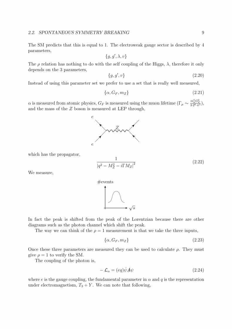
3·26·π3 ),and the mass of the Z boson is measured at LEP through,
e
e
Z
which has the propagator,1
|q2 −M2Z − iΓMZ |2
(2.22)
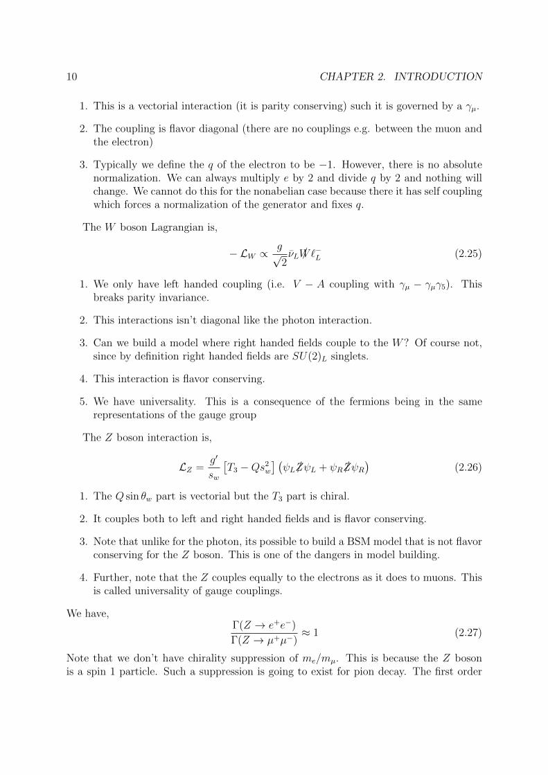
We measure,
#events
√s
In fact the peak is shifted from the peak of the Lorentzian because there are otherdiagrams such as the photon channel which shift the peak.
The way we can think of the ρ = 1 measurement is that we take the three inputs,
α,GF ,mZ (2.23)
Once these three parameters are measured they can be used to calculate ρ. They mustgive ρ = 1 to verify the SM.
The coupling of the photon is,
− Lα = (eq)ψ /Aψ (2.24)
where e is the gauge coupling, the fundamental parameter in α and q is the representationunder electromagnetism, T3 + Y . We can note that following,
10 CHAPTER 2. INTRODUCTION
1. This is a vectorial interaction (it is parity conserving) such it is governed by a γµ.
2. The coupling is flavor diagonal (there are no couplings e.g. between the muon andthe electron)
3. Typically we define the q of the electron to be −1. However, there is no absolutenormalization. We can always multiply e by 2 and divide q by 2 and nothing willchange. We cannot do this for the nonabelian case because there it has self couplingwhich forces a normalization of the generator and fixes q.
The W boson Lagrangian is,
− LW ∝g√2νL /W`−L (2.25)
1. We only have left handed coupling (i.e. V − A coupling with γµ − γµγ5). Thisbreaks parity invariance.
2. This interactions isn’t diagonal like the photon interaction.
3. Can we build a model where right handed fields couple to the W? Of course not,since by definition right handed fields are SU(2)L singlets.
4. This interaction is flavor conserving.
5. We have universality. This is a consequence of the fermions being in the samerepresentations of the gauge group
The Z boson interaction is,
LZ =g′
sw
[T3 −Qs2
w
] (ψL /ZψL + ψR /ZψR
)(2.26)
1. The Q sin θw part is vectorial but the T3 part is chiral.
2. It couples both to left and right handed fields and is flavor conserving.
3. Note that unlike for the photon, its possible to build a BSM model that is not flavorconserving for the Z boson. This is one of the dangers in model building.
4. Further, note that the Z couples equally to the electrons as it does to muons. Thisis called universality of gauge couplings.
We have,Γ(Z → e+e−)
Γ(Z → µ+µ−)≈ 1 (2.27)
Note that we don’t have chirality suppression of me/mµ. This is because the Z bosonis a spin 1 particle. Such a suppression is going to exist for pion decay. The first order
2.2. SPONTANEOUS SYMMETRY BREAKING 11
correction to this is due to the mass of the muon, mµ/MZ , which gives a larger phasespace to the electrons. A similar ratio is,
Γ(π+ → µ+ν)
Γ(π+ → e+ν)≈m2µ
m2e
(2.28)
However, in this case because of helicity suppression this ratio is about 104, while naivelyyou would expect the electron to have a larger branching ratio. The idea is the neutrinois only left chiral, while the charged lepton, because the decaying particle is a scalar mustthen have right handed helicity. But since the W only couples to left handed particlesyou need a left handed charged lepton to mix into a right handed charged lepton and thismixing is proportional to the mass. Therefore the suppression is,
∼(mµ
me
)2
∼ 4× 10⁴ (2.29)
which after accounting for the additional phase space of the electron is closer to 104. Thischirality suppression can be eliminated if a photon is also added into the final state.
The W boson quark coupling is given by,
− LW =g√2uiLγ
µVijdjLW
+µ + h.c. (2.30)
where Vij is the CKM matrix. This matrix encodes flavor and CP violation. The CKM has10 parameters. This is very peculiar since we started with 36 (18 for each Yukawa matrix).However, it turns out that many of these are unphysical. We now do this countingexpilcitly. To understand how to do this counting we take a detour into symmetries.
The global symmetries of the SM are,
U(1)B × U(1)e × U(1)µ × U(1)τ (2.31)
These symmetries are accidental, meaning that they are not imposed but a consequenceof the gauge group and field content. Note that such symmetries are only preserved atthe renormalizable level and hence are also a consequence of choosing to truncate theLagrangian at a given order.
Recall that the fermion Lagrangian is
L = Lkin + LY uk (2.32)
The symmetries of the kinetic term is much larger then the symmetries of the Yukawainteraction. As an example lets consider the kinetic term of the up type quarks,
Lukin = iU i /DU i (2.33)
This Lagrangian is invariant under an U(3) rotation between the up flavors (if U werereal then the symmetry would be O(3)). This rotation for example means if we want touse u and c as our light up type quarks we are equally well to use,
u± c√2
(2.34)
12 CHAPTER 2. INTRODUCTION
This symmetry is not satisfied by the Yukawa interaction because the Yukawas, YijQiφU j,
are not universal. After a rotation we have,
RkiYijRj`QkφU ` (2.35)
and in generalRkiYijRj` 6= Yk` (2.36)
This is a simple Lie group,U(3) = SU(3)× U(1) (2.37)
The global symmetry of the kinetic term of the quarks is given by,
U(3)Q × U(3)D × U(3)U (2.38)
Under these three global symmetries we have,
Q = (3, 1, 1) (2.39)
D = (1, 3, 1) (2.40)
U = (1, 1, 3) (2.41)
An important tool in this business is the spurion. A spurion is a number (not a field!)but we assign this number the transformation properties of some group. As an exampleconsider the Higgs. We can write the Higgs as,(
0v
)(2.42)
We can say this that this number transforms as a doublet under SU(2)L. We could havewritten this without ever knowing that the Higgs actually transforms in this way.
Now lets think of the Yukawas as spurions. Consider for example the quark Yukawa,
YUQUφ (2.43)
Under a flavor rotation we have,
YUQUφ→ R†QY′URUQUφ (2.44)
This term is invariant ifYU → RQYUR
†U (2.45)
i.e. ifYU = (3, 1, 3) (2.46)
Similarly we have,YD = (3, 3, 1) (2.47)
Even though this symmetry doesn’t exist in SM, its stil useful to know how terms breakthe symmetry. For example in the electroweak sector we still talk about SU(2) × U(1)
2.2. SPONTANEOUS SYMMETRY BREAKING 13
even though its broken. In the same way even though this flavor symmetry is broken westill use these spurion transformation properties.
We can finally move onto counting parameters. As an easy example lets consider theZeeman effect. There we put an atom in a magnetic field,
B = Bxx+Byy +Bz z (2.48)
In quantum mechanics classes we then move on and say the field is in the z direction.Why are we able to make this simplification? The answer is although its true we have 3parameters, we only have 1 physical parameter which is the magnitude of the magneticfield. We have,
# of param = 1 physical + 2 unphysical
The reason we were able to make this simplificaition is because of symmetry. The un-perturbed Hamiltonian is SO(3). After applying a magnetic field the symmetry becomesSO(2) (for us the unperturbed symmetry is that of the kinetic term and the perturbedone is the symmetry of the Yukawa interaction). We reduced the symmetry of the prob-lem by applying the magnetic field. SO(3) has 3 generators, while SO(2) has only one.Therefore we broke 2 generators. We can use the broken generators to rotate away un-physical parameters. In this case rotate around x and y axes to eliminate Bx and By.We always have,
# of phys param = # total−# broken gen
Lets consider the number of parameters in the up type quark sector. The initialsymmetry was U(3)Q × U(3)U × U(3)D which has 9 + 9 + 9 = 27 parameters. The finalsymmetry is U(1) which has 1 parameter. Therefore there are 26 broken generators. Thetotal number of parameters is
3 × 3︸ ︷︷ ︸3 by 3 mat.
×Re + Im︷︸︸︷
2 × 2︸︷︷︸up+down
= 36 . (2.49)
Therefore there are 36− 26 = 10 physical parameters, 6 quark masses, 3 mixing angles,and 1 phase. You can even find how many real and how many imaginary parameters.The yukawa matrices had 18 real and 18 imaginary parameters. The U(3) matrices have5 real parameter and 4 imaginary (recall there are 5 real Gell-mann matices) resultingin 15 broken real generators and 11 broken imaginary generators (U(1)B is an unbrokenimaginary generator). This gives, 18 − 15 = 3 real parameters in the quark sector and18− 11 = 7 imaginary parameters.
Lets do the same trick for the lepton. The initial symmetry is U(3)L×U(3)E which has18 parameters and the final symmetry is U(1)e×U(1)µ×U(1)τ which has 3 parameters.Therefore the number of physical parameters is,
18− (18− 3) = 3 (2.50)
These are just the lepton masses since in the SM we don’t have a PMNS matrix (and noneutrino masses).
14 CHAPTER 2. INTRODUCTION
2.3 Beyond the Standard Model
Problems with the Standard Model can be divided into two types “data” and “beauty”.Data problems are the traditional type of problem in science, however, theoretical highenergy physics also has beauty or hierarchy problems.
1. Gravity - “theoretical problem”
2. Hierarchy problems
3. Data - neutrino masses, dark matter, dark energy, baryogenesis, inflation
The hierarchy problems in the SM are as follows:
1. mφ MPl - “10−16 problem“
2. Flavor puzzle - “ 10−6”
3. Strong CP problem - “10−10”
4. Cosmological constant problem - “10−120”
5. Gauge unification
Fine tunings can take two distinct form, problems which are “technically natural”(e.g., the flavor problem) or not-“technically natural” (e.g., the hierarchy problem). Asmall number is technical natural if a symmetry is restored in the limit that the numbergoes to zero. For example consider the mass of the electron. In the limit that me → 0,QED has a new symmetry, a chiral symmetry, e → eiγ5e. This is not true for the SMhiggs mass. This feature is important because any corrections to the parameter mustthen be proportional to the parameter. For example,
m1-loope = mtree
e (log(...)...) (2.51)
(m1-looph )2 = Λ2(log(...) + ...) (2.52)
The higgs mass corrections are proportional to the physics at the UV while the electronmass corrections are proportional to the electron. If there is a solution to a technicallynatural problem it can live at any scale, problems that are not technically natural mustbe solved at the scale of the parameter.
We can write the SM Lagrangian as,
LSM = LR︸︷︷︸renormalizable
+ L(5) + L(6) + ...︸ ︷︷ ︸nonrenormalizable
(2.53)
There is a single unique dimension five operator in the SM,
L(5) =(LH)2
Λ(2.54)
2.3. BEYOND THE STANDARD MODEL 15
There is of order 100 new operators that can show up at dimension six,
L(6) =OΛ2
(2.55)
One such operator is,uRuRdReR (2.56)
This will give rapid proton decay and spoils the first success that we listed of SM. Toavoid this term we have two options,
1. Impose a symmetry (e.g. R parity)
2. Take Λ v.
3. Approximate symmetry
Chapter 3
Electroweak Precision
For this section we use the references,
1. Peskin - chapter 22
2. PDG
3. hep-ph/0412166
4. Skiba - TASI 2009
In electroweak we have,SU(2)L × U(1)Y → U(1)EM (3.1)
and its charatorized byg, g′, v (3.2)
These 3 parameters completely describe the electroweak sector of the SM at tree level.Basically what we want to do is overconstrain these three parameters and test our theory.At tree level the gauge sector is governed by only three parameters. After loop correctionswe have to worry about more parameters due to new processes happening at one loop.The most important parameters that are going to be important are the ones that arelarge,
mh,mt, gs (3.3)
As an example of electroweak prceision (EWP) lets think about how to measure theweinberg angle. There are three ways to define the Weinberg angle. The first two are,
sin2 θW = 1− m2W
m2Z
(3.4)
sin2 2θ0 =4πα(m2
Z)√2GF (m2
µ)m2Z
(3.5)
The capital W on θW reminds us that this definition arises from the mass of the W bosonand not just the weinberg angle and the 0 subscript is just conventional.
16
17
The third definition arises from the coupling of the Z to the fermions which is givenby,
LψiψiZ = − g
2 cos θwψiγµ
(giV − giAγ5
)ψiZ
µ (3.6)
then 1,
gV = T3 − 2q sin2 θ∗ (3.8)
gA = T3 (3.9)
Taking the difference of these equations and dividing by 2qi we get,
sin2 θi∗ ≡giA − giV
2qi(3.10)
In principle we have 9 of these definitions of the Weinberg angle (one for each fermionwhich is charged) and so θ∗ should have a flavor index on it. But to leading order thecorrection is universal. The best way to measure the θ∗ is to use polarization informationsince then it differentiates gV from gA.
To find the corrections to the different definitions we consider the corrections to thepropagator (these will effect the mass of the gauge bosons and hence the weinberg angles).
1.Z → `+`− (3.11)
This only works for the b or τ since they decay and then you can measure theirpolarization from the angular distributions. But you it doesn’t work for the otherflavors.
2. One can polarize e+e− → Z as was done at SLAC.
When we talk about oblique corrections we mean corrections that are the same for allthe flavors.
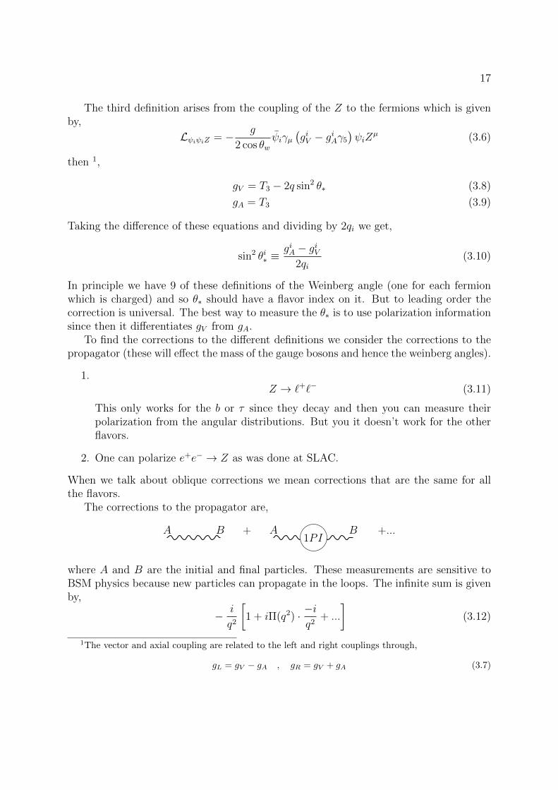
The corrections to the propagator are,
A B + A B1PI
+...
where A and B are the initial and final particles. These measurements are sensitive toBSM physics because new particles can propagate in the loops. The infinite sum is givenby,
− i
q2
[1 + iΠ(q2) · −i
q2+ ...
](3.12)
1The vector and axial coupling are related to the left and right couplings through,
gL = gV − gA , gR = gV + gA (3.7)
18 CHAPTER 3. ELECTROWEAK PRECISION
Here we are being a little hasty. Outside of QED it is not clear what exactly is meant byΠ(q2) since in general the propagator correction is,
ΠµνAB(q2) = ΠAB(q2)gµν −∆(q2)qµqν (3.13)
We define the scalar, ΠAB(q2) as the quantity preceding the gµν in the propagator cor-rection. In the results that follow the ∆ dependent terms will always be proportionalto
qµjµ = 0 (3.14)
due to gauge invariance. Therefore, we can drop this contribution for the purposes of ourdiscussion.
We can work in either the physical basis,
W±, γ, Z
(3.15)
or in the unphysical basis, W+,W 3, B
(3.16)
In general we have four propagator that we need to calculate,
ΠW−W− ,ΠW+W+ ,Πγγ,ΠZZ (3.17)
We now make the assumption that we work in a region with small q2 compared tothe heavy particles,
Π(q2) = Π(0) + q2Π′(0) + ... (3.18)
We have the identities,
m2W = m
(tree) 2W + ΠWW (m2
W ) (3.19)
Πγγ(0) = 0 (3.20)
ΠγZ(0) = ΠγZ(m2Z) = 0 (3.21)
where the last two identities follow since particles can only mix while both particles areoff-shell. [Q 1: I don’t think the last identity is true, ΠγZ(m2
Z) = 0 since we use it later...]
This isn’t a very good assumption for the massive gauge bosons mass corrections (theyare about a factor of 2 ligher then the top), but a terrific one for the photon propagatorcorrection
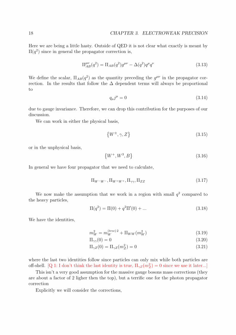
Explicitly we will consider the corrections,
19
a)
W Wb
t
b)
Z Zb, t
b, t
c)
γ γ
b, t
b, t
d) µ
νµ
e)
Z γ
b, t
b, t
Note that (a) and (d) are really same calculation however we write them separately sincethey are evaluated at different q2. (a) is evaluated at the Higgs mass while (d) is evaluatedat the muon mass.
Lets consider these corrections. The massive gauge boson masses are,
m2W =
g2v2
4+ ΠWW (mZ) (3.22)
m2Z =
(g2 + g′2)v2
4+ ΠZZ(mZ) (3.23)
Then we can calculate θW (the “W boson weinberg angle”),
sin2 θW = 1−m2W,0 + ΠWW
m2Z,0 + ΠZZ
(3.24)
= sin2 θ︸ ︷︷ ︸tree level result
− 1
m2Z
[ΠWW − cos2 θΠZZ
](3.25)
where cos2 θ is just the tree level result since the corrections to this are a higher ordereffect, and we used a subscript 0 to denote the tree level masses. ΠAB is calulated inappendix 3.A. Lets try to study the divergences of diagram (a). The diagram is roughlygiven by,
∼∫
d4k(/k +m)(/k +m)
(k2 +m2)2∼∫d4k
k2∼ Λ2 (3.26)
However, this divergence is artificial and isn’t existent due to the Ward identity. It maynot be obvious that the massive gauge boson still is protected by a Ward identity butit turns out to be the case. The intuition behind this is that the UV divergence doesn’t
20 CHAPTER 3. ELECTROWEAK PRECISION
see the masses of the particles (at very large momenta you can set the masses to zero).However, there is a log divergence2. However, the divergence between two definitions ofθ always cancels.
The calculation for θW was relatively easy since the modifications of mW and mZ areobvious. This isn’t always the case. To find the correction to θ∗ we need the correctionto α,GF , and mW . To find the corrections for α recall that due to gauge invariance wehave3,
e =√
1 + Π(q2)/q2e0 (3.27)
Taylor expanding the propagator we have,
Π(q2) ≈[*0
Π(0) + q2Π′(0) + ...
](3.28)
where the first term vanishes due to gauge invariance and we drop terms of order q4/m4t .
Rewriting in terms of the fine structure constant we have,
4πα =g2g′2
g2 + g′2(1 + Π′γγ(0)
)(3.29)
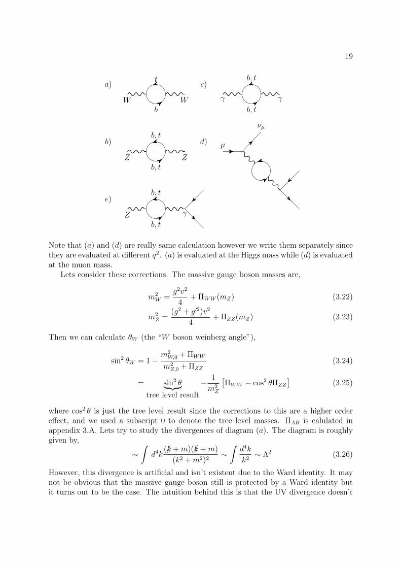
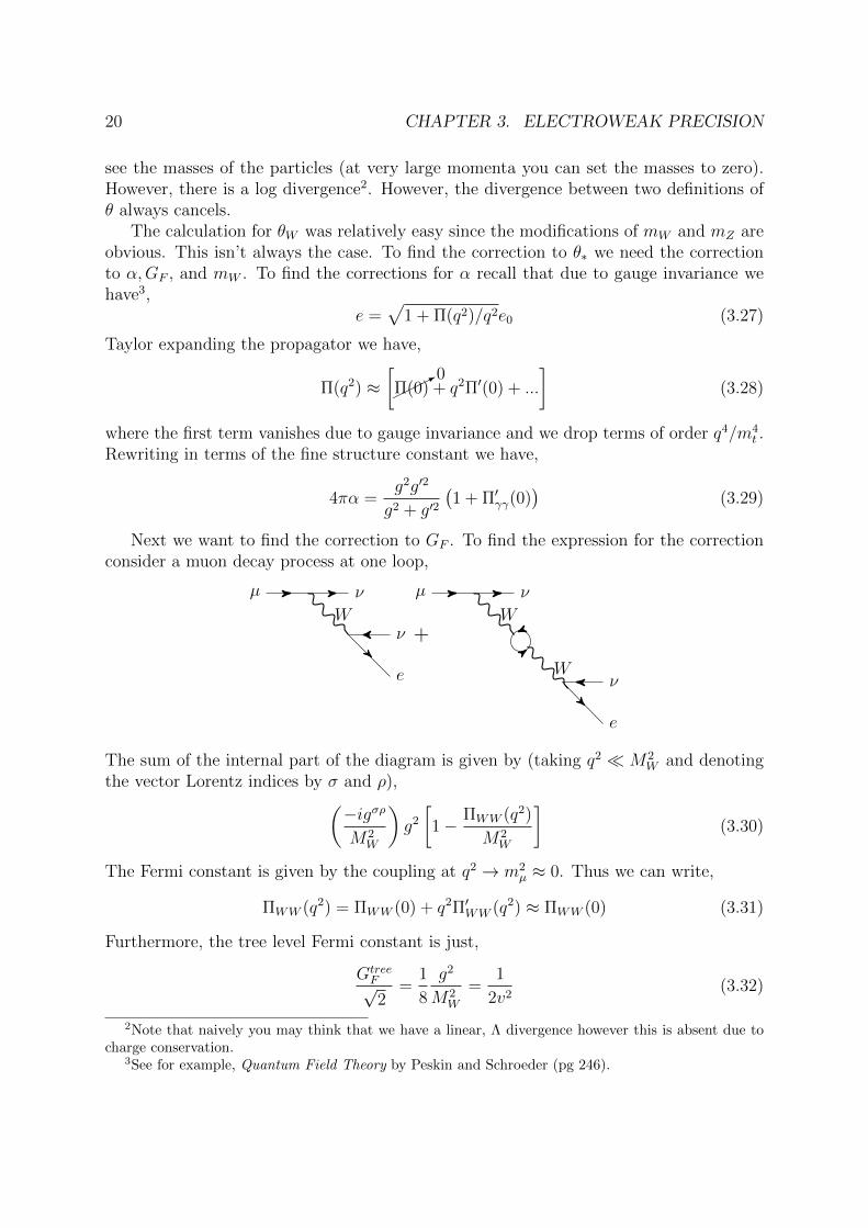
Next we want to find the correction to GF . To find the expression for the correctionconsider a muon decay process at one loop,
µ ν
W
e
ν +
µ ν
W
W
e
ν
The sum of the internal part of the diagram is given by (taking q2 M2W and denoting
the vector Lorentz indices by σ and ρ),(−igσρ
M2W
)g2
[1− ΠWW (q2)
M2W
](3.30)
The Fermi constant is given by the coupling at q2 → m2µ ≈ 0. Thus we can write,
ΠWW (q2) = ΠWW (0) + q2Π′WW (q2) ≈ ΠWW (0) (3.31)
Furthermore, the tree level Fermi constant is just,
GtreeF√2
=1
8
g2
M2W
=1
2v2(3.32)
2Note that naively you may think that we have a linear, Λ divergence however this is absent due tocharge conservation.
3See for example, Quantum Field Theory by Peskin and Schroeder (pg 246).
21
Therefore the sum of the diagrams is,
− i8GtreeF√2gσρ[1− ΠWW (0)
m2W
](3.33)
which implies thatGF√
2=
1
2v2
[1− ΠWW (0)
M2W
](3.34)
We are finally in position to calculate sin2 2θ0 at one loop. Using equation 3.5,
sin2 2θ0 =g′2
g2 + g′2(1 + Π′γγ(m
2Z)) [ 1
v2
(1− ΠWW (0)
M2W
)((g2 + g′2)v2
4+ ΠZZ(m2
Z)
)]−1
(3.35)
=4g′2g2
(g2 + g′2)2
[1 + Π′γγ(0) +
ΠWW (0)
M2W
− ΠZZ(0)
m2Z
](3.36)
where the factor in front is just another way of writing sin2 2θw at tree level. While thisexpression is perfectly fine it is more convenient to have an expression for sin2 θ0. To findthe new expression we make the convenient definitions,
A ≡ 4 sin2 2θw ε ≡ Π′γγ(0) +ΠWW (0)
M2W
− ΠZZ(0)
m2Z
(3.37)
Then we have,sin2 θ0
(1− sin2 θ0
)= A(1 + ε) (3.38)
which after using the quadratic equation give,
sin2 θ0 =1
2
(1±
√1− 4A(1 + ε)
)(3.39)
for θw ≈ 20o the physical root is the negative one. Identifying 1−√
1− 4A with sin2 θwwe have,
sin2 θ0 = sin2 θw +cos2 θ sin2 θ
cos 2θ
[Π′γγ(0) +
ΠWW (0)
M2W
− ΠZZ(0)
m2Z
](3.40)
In an analogous way to the calculation leading to equation 3.25 one can show that,
sin2 θ∗ − sin2 θtree = −sin θ cos θΠγZ (m2Z)
m2Z
(3.41)
An explicit calculation gives
sin2 θ0 − sin2 θ∗ =3α
16π cos2 2θ
m2t
m2Z
(3.42)
sin2 θW − sin2 θ∗ =−3α
16π sin2 θ
m2t
m2Z
(3.43)
22 CHAPTER 3. ELECTROWEAK PRECISION
where we have only kept terms quadratic in mt. Note that differences of quantities thatyou renormalize is finite. This is always the case since the differences of two renormalizedquantities is physical. This is analogous to absolute energies being unphysical but energydifferences are physical. This is a prime example of how you can get sensitivity to a heavyparticle (the top in this case) at one loop. We see that this result appears to violate thedecoupling theorem which says that as the mass of a particle is taken to infinity it shoulddissapear from the theory. However, this is not true since taking the mass here to infinitywould require taking the Yukawa coupling to infinity which is impossible since it wouldmake the theory nonperturbative.
Through these types of calculations we were able to predict the mass of the top to bearound 150GeV which was correct within 1σ. One can calculate the corresponding Higgscorrection to this quantity such a correction gives,
s20 − s2
θ =3α
16π cos2 2θ
m2t
m2Z
+ # log(mH
mZ
) (3.44)
The Higgs correction surprisingly is going to logarithmic. This is a unique one loopeffect and is due to the fact that the Higgs is not just a regular scalar but the particlewhich breaks spontaneous symmetry breaking. This logarithm reduces the effectivenessin predicting the mass of the Higgs.
The general philosophy is to look at many different measurements as the one above.After you are done you can make a fit between all these results and estimate each pa-rameter. This is done in the Gfitter website.
We can divide the actual measurements into two types of data, low energy and highenergy data. For low energy data we have neutrino scattering. Basically you take aneutrino and you scatter it off a wall and you see the ejected electron moving. Thesensitivity to these sorts of interactions is due to coupling to the Z. Other low energymeasurements arise from parity violating atomic physics as well of course measurementsof GF , α, g − 2, ....
High energy data arose from LEP and SLAC. They calculated, mZ ,ΓZ ,ΓZ→had,ΓZ→νν ,and Afb. More recent high energy data arises from hadron colliders which aren’t verygood for precision measurements but designed for discovery instead.
3.1 Neutral Currents
Prior to discovery of the Z boson people thought about whether such a boson reallyexists. At this point people only new of the four fermi interaction which only couples left
chiral fields. In fact you can build a model with SU(2)SSB−−→ U(1)EM which will just have
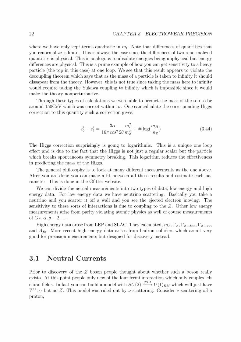
W±, γ but no Z. This model was ruled out by ν scattering. Consider ν scattering off aproton,
3.2. ATOMIC PARITY VIOLATION 23
ν ν
Z
The signiture would be a proton in a sheet getting a kick due to a neutrino beam. Onecan device a similar experiment for scattering off an electron,
ν ν
ee
Z
These involve a low energy Z exchange. The only time a low energy Z will be importantwill be when we use neutrinos since they don’t interact with the photon.The cross-sectionfor interaction with an electron is,
σ =GFmeEν
2π
[(gV ± gα)2 +
1
3(gV ∓ gA)2
](3.45)
To calculate gV and gA you can take the ratio of different neutrino flavor interactions.
3.2 Atomic parity violation
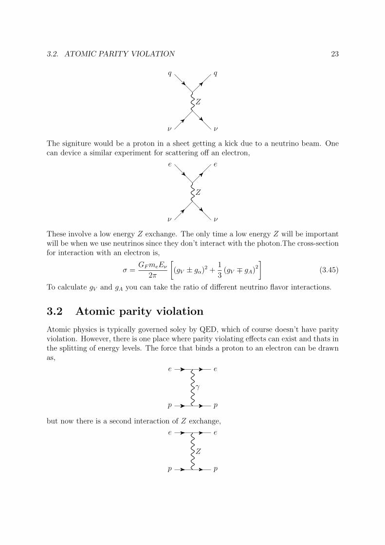
Atomic physics is typically governed soley by QED, which of course doesn’t have parityviolation. However, there is one place where parity violating effects can exist and thats inthe splitting of energy levels. The force that binds a proton to an electron can be drawnas,
ee
γ
p p
but now there is a second interaction of Z exchange,
ee
Z
p p
24 CHAPTER 3. ELECTROWEAK PRECISION
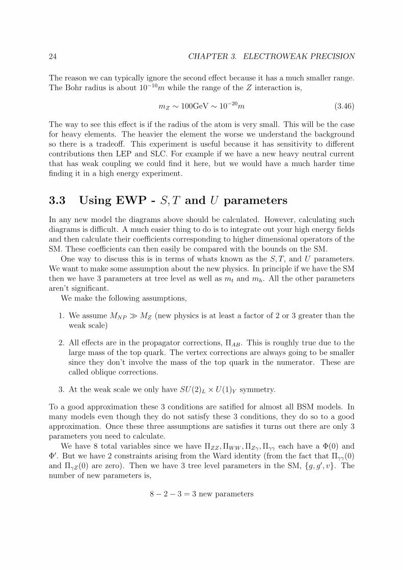
The reason we can typically ignore the second effect because it has a much smaller range.The Bohr radius is about 10−10m while the range of the Z interaction is,
mZ ∼ 100GeV ∼ 10−20m (3.46)
The way to see this effect is if the radius of the atom is very small. This will be the casefor heavy elements. The heavier the element the worse we understand the backgroundso there is a tradeoff. This experiment is useful because it has sensitivity to differentcontributions then LEP and SLC. For example if we have a new heavy neutral currentthat has weak coupling we could find it here, but we would have a much harder timefinding it in a high energy experiment.
3.3 Using EWP - S, T and U parameters
In any new model the diagrams above should be calculated. However, calculating suchdiagrams is difficult. A much easier thing to do is to integrate out your high energy fieldsand then calculate their coefficients corresponding to higher dimensional operators of theSM. These coefficients can then easily be compared with the bounds on the SM.
One way to discuss this is in terms of whats known as the S, T, and U parameters.We want to make some assumption about the new physics. In principle if we have the SMthen we have 3 parameters at tree level as well as mt and mh. All the other parametersaren’t significant.
We make the following assumptions,
1. We assume MNP MZ (new physics is at least a factor of 2 or 3 greater than theweak scale)
2. All effects are in the propagator corrections, ΠAB. This is roughly true due to thelarge mass of the top quark. The vertex corrections are always going to be smallersince they don’t involve the mass of the top quark in the numerator. These arecalled oblique corrections.
3. At the weak scale we only have SU(2)L × U(1)Y symmetry.
To a good approximation these 3 conditions are satified for almost all BSM models. Inmany models even though they do not satisfy these 3 conditions, they do so to a goodapproximation. Once these three assumptions are satisfies it turns out there are only 3parameters you need to calculate.
We have 8 total variables since we have ΠZZ ,ΠWW ,ΠZγ,Πγγ each have a Φ(0) andΦ′. But we have 2 constraints arising from the Ward identity (from the fact that Πγγ(0)and ΠγZ(0) are zero). Then we have 3 tree level parameters in the SM, g, g′, v. Thenumber of new parameters is,
8− 2− 3 = 3 new parameters
3.3. USING EWP - S, T AND U PARAMETERS 25
We define,
T ≡ 1
α
[ΠWW
m2W
− ΠZZ
m2Z
](3.47)
S ≡ 4 sin2 2θ
α
[Π′ZZ −
2 cos2 2θ
sin2 2θΠ′Zγ − Π′γγ
](3.48)
U ≡ 4 sin2 θ
α
[Π′WW − cos2 θΠ′ZZ − sin 2θΠ′Zγ − sin2 θΠ′γγ
](3.49)
[Q 2: Which θ do we use?]A few remarks:
1. This is not really the proper definition. In the real definition you add a constantsuch that the SM value of T, S, U is zero.
2. The T parameter is closely related to the ρ− ρSM parameter.
3. Practically we never hear about U , we only hear about T and S. The reason is thatwhen you write these parameters in terms of higher dimensional operators, T andS are dimension 6 while U is dimension 8.
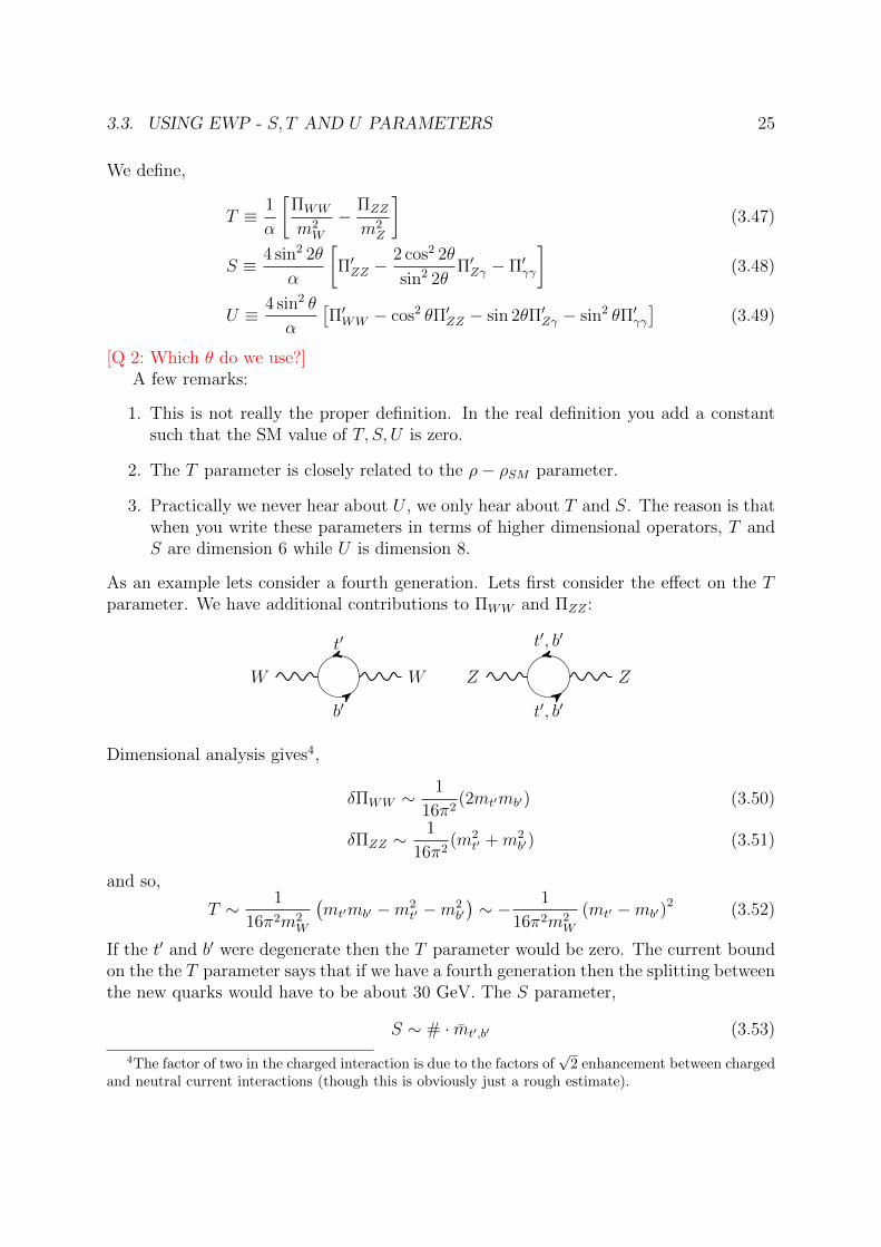
As an example lets consider a fourth generation. Lets first consider the effect on the Tparameter. We have additional contributions to ΠWW and ΠZZ :
W
t′
b′
W Z
t′, b′
t′, b′
Z
Dimensional analysis gives4,
δΠWW ∼1
16π2(2mt′mb′) (3.50)
δΠZZ ∼1
16π2(m2
t′ +m2b′) (3.51)
and so,
T ∼ 1
16π2m2W
(mt′mb′ −m2
t′ −m2b′
)∼ − 1
16π2m2W
(mt′ −mb′)2 (3.52)
If the t′ and b′ were degenerate then the T parameter would be zero. The current boundon the the T parameter says that if we have a fourth generation then the splitting betweenthe new quarks would have to be about 30 GeV. The S parameter,
S ∼ # · mt′,b′ (3.53)
4The factor of two in the charged interaction is due to the factors of√
2 enhancement between chargedand neutral current interactions (though this is obviously just a rough estimate).
26 CHAPTER 3. ELECTROWEAK PRECISION
where # is roughly the number of particles. This parameter essentially counts howmany new generations you have. The S parameter has actually already ruled out sucha possibility except for peculiar regions of parameter space. Note that the bounds onadditional scalars are about 6 times weaker. This is why SUSY is still within thesebounds.
3.4 Custodial symmetry
The custodial symmetry is an accidental symmetry which is only of the Higgs sector. Fora extensive discussion on custodial symmetry, see 0410370 Here we outline the importantpoints.
Consider the Higgs potential in the SM,
V = −µ2φ†φ+ λ(φ†φ)2 (3.54)
The Higgs doublet takes the explicit form 5,
φ =
(φ1 + iφ2
φ3 + iφ4
)=
(φ+
φ0
)φ ≡ εφ∗ =
(φ0∗
−φ−)
(3.55)
But the only variable in the potential is given by,
φ†φ = φ21 + φ2
2 + φ23 + φ2
4 (3.56)
Since the potential depends only on the length of a four dimensional vector, there isactually a larger symmetry, SO(4) ∼ SU(2)⊗ SU(2). The length after SSB is given by,
φ†φ→ (φ1 + v)2 + φ22 + φ2
3 + φ24 (3.57)
Since there is still a rotational symmetry about φ2, φ3, φ4 there is a residual SO(3) sym-metry. Therefore we have,
SO(4)→ SO(3) ∼ SU(2)D (3.58)
where the D stands for “diagonal”. This SU(2)D is what we call custodial symmetry.Its easier to discuss this symmetry if we combine the Higgs, φ, and its conjugtate, φ,
into a matrix representation. We define6,
Φ =1√2
(φ φ
)(3.59)
5Recall that φ isn’t an independent degree of freedom but just a convenient way to form SU(2)Ldoublets out of a Higgs with opposite hypercharge.
6Alternatively, one can think of projecting the Higgs vector,(φ1 φ2 φ3
)Tonto the Pauli matrices
and then switching the charged basis.
3.4. CUSTODIAL SYMMETRY 27
Note that,
Φ†Φ =1
2
(φ†φ φ†φ
φ†φ φ†φ
)⇒ Tr
[Φ†Φ
]= φ†φ (3.60)
where we have used the fact that φ†φ = φ†φ. Deriving the kinetic term is more involvedand the derivation is shown in appendix 3.B. The Higgs Lagrangian is given by,
LHiggs = TrDµΦ†DµΦ− µ2Tr[Φ†Φ
]+ λTr
[Φ†Φ
](3.61)
where the covariant derivative takes the form,
DµΦ = ∂µΦ− i
2gW a
µσaΦ +
i
2g′BµΦσ3 (3.62)
Note the extra σ3 on the hypercharge term which is a consequence of φ and φ havingdifferent hyperchanges. Furthermore, note that σ3 multiplies Φ from the right.
Since φ and φ both transform as doublets under SU(2)L we can write,
Φ =1√2
(φ φ
)→ L
1√2
(φ φ
)(3.63)
while we the usual global transformation for the gauge field, W µ → LW µL†. The scalarpotential, which is made out of TrΦ†Φ is trivially invariant under SU(2)L. For the kineticterm we have,
Tr∂µΦ†∂µΦ→ Tr∂µΦL†L∂µΦ (3.64)
Tr∂µΦ†W µa σ
aΦ→ Tr∂µΦ†L†LW µa L†LΦ (3.65)
Tr∂µΦ†BµΦσ3 → Tr∂µΦ†L†LBµΦσ3 (3.66)
etc.Note however, that due to the trace we almost have another symmetry, Φ → ΦR†,
where R is an SU(2) transformation. The symmetry breaking term is the g′ contribution.For example,
Tr∂µΦ†BµΦσ3 → Tr∂µΦ†BµΦR†σ3R (3.67)
where we have the extra factor, R†σ3R 6= σ3.This symmetry is also broken by the Yukawa interactions which in our notation take
the form,
Tr
[(t†L b†Lt†L b†L
)(φ0∗ φ+
φ− φ0
)(yt 00 yb
)(tR 00 bR
)](3.68)
The downtype quarks aren’t made of SU(2) multiplets so we can’t just let them trans-form analagously to the tL, bL fields to keep the Yukawas invariant under the custodialsymmetry.
We can identify one of the SU(2) as the gauge symmetry. The symmetry of the theoryis given by,
SU(2)L ⊗ SU(2)R (3.69)
28 CHAPTER 3. ELECTROWEAK PRECISION
SU(2)L is easy to identify. SU(2)R contains U(1)Y and two other global symmetrygenerators (i.e. they are not gauged). Note that in a left right symmetric theory thisSU(2)R is also gauged. The Higgs transforms as,
Φ→ LΦR† (3.70)
The VEV of the Higgs takes the form,
〈Φ〉 =1
2
(v 00 v
)(3.71)
This is not invariant under SU(2)L or SU(2)R (its easy to see that L 〈Φ〉 6= 〈Φ〉, andsimilarly for SU(2)R). However, it is invariant under transformations such that L = R.We say that the resultant theory is invariant under diagonal or vector transformations,
〈Φ〉 → D 〈Φ〉D† = 〈Φ〉 (3.72)
The W aµ gauge bosons transform as a triplet under SU(2)L and a singlet under SU(2)R
because forming a singlet out of TrDµΦ†DµΦ relies on the W µ remaining underchangedunder SU(2)R and using the trace to cycle the transformation matrices. Therefore, theymust transform as a triplet under SU(2)D.
In the limit that g′ = 0 we have 3 massive degenerate gauge bosons and one masslessphoton. Moving away from this limit, one boson remains massless while there is a splittingbetween the remaining 3. We have,
m2W =
1
4g2v2 m2
Z =1
4(g2 + g′2)v2 (3.73)
We also have the mixing angle,
cos2 θw =g2
g2 + g′2(3.74)
which controls how far we are from the g′ = 0 limit (g′ = 0 → cos2 θw = 1). However, westill have the equality mW3 = mW1,2 . This results in the famous SM tree level prediction,
ρ ≡ m2W
m2Z cos2 θw
= 1 (3.75)
where mW3 ≡ mZ cos θw and mW = mW1 = mW2 as these masses are unaffected by therotation in the neutral sector. The ρ = 1 relation is a consequence of the custodial sym-metry since this is what gaurentees that mW1,2 = mW3 . If we had a higher representationof the Higgs then the masses of the W bosons would be different. In general each com-ponent of the W couples to a different combination of φi. Each of them gets a fractionof the VEV.
Since the custodial symmetry is broken by both the Yukawa interactions as well asg′, radiative corrections to the ρ = 1 relation must be either proportional to the splittingof the quarks or g′.
3.5. HIGHER DIMENSIONAL OPERATORS 29
3.5 Higher dimensional operators
This analysis follows hep-ph/0412166.
If you keep all the flavor indices in the SM then there are 2499 dimension 6 operators.If you forget about flavor indices there are 80 operators. However, it turns out that youcan use the equations of motion to eliminate some of the operators. This reduces thenumber of operators to 59. Many of these still don’t affect EWP but are only relevantin flavor physics. This is because the bounds from KK mixing are much stronger thenfrom EWP. This brings us to only 28 dimension 6 operators.If you check what the datais sensitive to there are only 21 operators.
In the reference above they took the 21 operators and they found the matrix of bounds.So in your new physics model you can calculate all the 21 operators and compare withthese bounds. Out of all these operators the most important ones are
S ↔ OWB ≡H†W µνBµνH
Λ2(3.76)
T ↔ OH ≡∣∣H†DµH
∣∣2Λ2
(3.77)
Y ↔ OBB ≡(DµB
µν)2
Λ2(3.78)
W ↔ OWW ≡(DµW
µν)2
Λ2(3.79)
where the letters on the left indicate a name for these operators. [Q 3: There is somesubtlety associated with how one defines Wµν . Look this up and comment.]
After electroweak symmetry breaking we can charactorize what symmetries the oper-ators break:
Custodial SU(2)LS + −T − −Y + +W + +
where a + (−) indicates that it conserves (doesn’t conserve) the symmetry. Note thatoperators that break a symmetry are much easier to probe. This is a very general propertysince in channels that break a symmetry we have lower backgrounds. This is for examplethe reason why we can probe the hyperfine splitting very precisely. With this in mindwe see that T is the most important parameter while S is the second most importantparameter for EWP.
We have two different expansions that we can consider. The first one is in our energyscale divded by the heavy physics energy scale. The other thing we can do is expand inq2 instead. For example in the muon decay,
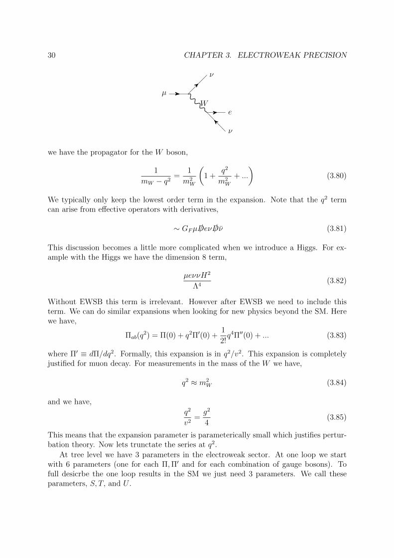
30 CHAPTER 3. ELECTROWEAK PRECISION
µ
ν
We
ν
we have the propagator for the W boson,
1
mW − q2=
1
m2W
(1 +
q2
m2W
+ ...
)(3.80)
We typically only keep the lowest order term in the expansion. Note that the q2 termcan arise from effective operators with derivatives,
∼ GFµ /Deν /Dν (3.81)
This discussion becomes a little more complicated when we introduce a Higgs. For ex-ample with the Higgs we have the dimension 8 term,
µeννH2
Λ4(3.82)
Without EWSB this term is irrelevant. However after EWSB we need to include thisterm. We can do similar expansions when looking for new physics beyond the SM. Herewe have,
Πab(q2) = Π(0) + q2Π′(0) +
1
2!q4Π′′(0) + ... (3.83)
where Π′ ≡ dΠ/dq2. Formally, this expansion is in q2/v2. This expansion is completelyjustified for muon decay. For measurements in the mass of the W we have,
q2 ≈ m2W (3.84)
and we have,
q2
v2=g2
4(3.85)
This means that the expansion parameter is parameterically small which justifies pertur-bation theory. Now lets trunctate the series at q2.
At tree level we have 3 parameters in the electroweak sector. At one loop we startwith 6 parameters (one for each Π,Π′ and for each combination of gauge bosons). Tofull desicrbe the one loop results in the SM we just need 3 parameters. We call theseparameters, S, T, and U .
3.5. HIGHER DIMENSIONAL OPERATORS 31
We can relate the Π’s to the couplings,
g−2 = Π′W+W− (3.86)
g′−2 = Π′BB (3.87)
v2 = −2ΠW+W− (3.88)
g−2m2W T = Π33 − ΠW+W− (3.89)
g−2S = Π′3B (3.90)
g−2U = Π′33 − Π′W+W− (3.91)
We define the “hatted” operators as rescaled versions of the operators we defined earlier,
S =4 sin2 θwS
αT =
T
αU = −4 sin2 θwU
α(3.92)
Unlike S and T , U doesn’t arise from a dimension 6 operator. Y and W which wementioned last time don’t break any symmetries.
If we keep one more order in q2 we have Π′′ and we need four more parameterswhich we call V (dim10)X(dim8)Y (dim6)W (dim6). In Π′′′ there are no more dimension6 operators.
There is another seminal paper in this field, Arxiv: 0007265. In this paper they justcalculate each operator one at a time. There they the bounds on these operators aregiven by,
OS ⇒ Λ & 10TeV (3.93)
OT ⇒ Λ & 5TeV (3.94)
This for example implies that in Randal Sundrum models (this is not 10 TeV becauseof a coupling),
mKK & 3TeV (3.95)
(the reason we have 3TeV and not 10TeV is because we have some couplings here). Asanother example supersymmetry is affected by these bounds. However, because super-symmetric particles must appear in loops, these bounds are reduced by factors of 16π2.
A last example of the utility of EWP is looking at a fourth generation. In that casewe introduce a t′, b′, e′, ν ′. The CKM becomes,
0VCKM 0
00 0 0 1
(3.96)
The masses of the new quarks are mt′ and mb′ . The T parameter is sensitive to breakingof the custodial symmetry so we would depend on the difference in their masses,
T ≈ Nc
12π sin2 θw cos2 θw
m2t′ −m2
b′
m2Z
(3.97)
32 CHAPTER 3. ELECTROWEAK PRECISION
Due to the boudns of the T parameter we have to assume the new generation is roughlygenerate. However the S is just a number,
S ≈ Nc
6π
(1− Y log
m2t′
m2b′
)≈ Nc
6π(3.98)
We say that S essentially counts the number of new flavors because for each new genera-tion we would get a contribution of about Nc/16π to the S parameter. The factor of Nc
is equal to 3 for the quarks and 1 for the leptons. Lastly, note that this doesn’t obey thedecoupling limit. This is because we are assuming the fourth generation couples to theHiggs and the coupling is bounded at 4π.
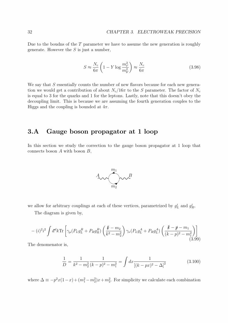
3.A Gauge boson propagator at 1 loop
In this section we study the correction to the gauge boson propagator at 1 loop thatconnects boson A with boson B,
A
m1
m2
B
we allow for arbitrary couplings at each of these vertices, parametrized by giL and giR,
The diagram is given by,
− (i)2i2∫ddkTr
[γµ(PLg
BL + PRg
BR)
(/k −m2
k2 −m22
)γν(PLg
AL + PRg
AL )
(/k − /p−m1
(k − p)2 −m21
)](3.99)
The denomenator is,
1
D=
1
k2 −m22
1
(k − p)2 −m21
=
∫dx
1
[(k − px)2 −∆]2(3.100)
where ∆ ≡ −p2x(1−x)+(m21−m2
2)x+m22. For simplicity we calculate each combination
3.A. GAUGE BOSON PROPAGATOR AT 1 LOOP 33
of left right projection operator simulataneously. We define a, b = ±1 and then we have,
Tr [...] =1
4
Tr[γµ(/k −m2)γν(/k − /p−m1)
]+ aTr
[γµγ
5(/k −m2)γν(/k − /p−m1)]
bTr[γµ(/k −m2)γνγ
5(/k − /p−m1)]
+ abTr[γµγ
5(/k −m2)γνγ5(/k − /p−m1)
](3.101)
=1
4
(1 + ab)Tr
[γµ/kγν(/k − /p)
]+ (1− ab)m1m2Tr [γµγν ]
− (a+ b)Tr[γµ/kγν(/k − /p)γ5
](3.102)
= (1 + ab) (kµ(k − p)ν − gµνk · (k − p) + (k − p)µkν) + (1− ab)m1m2gµν
+ (a+ b)iεµσνρkσ(k − p)ρ (3.103)
Shifting the integration variable and dropping terms linear in kµ we have,
Tr [...] = (1 + ab)(2kµkν − 2pµpν(1− x)x− gµν(k2 − p2x(1− x))
)+ (1− ab)m1m2gµν
(3.104)where the εµσνρ term doesn’t contribute since it multiplies a symmetric term. The relevantintegrals are, ∫
ddkkµkν
(k2 −∆)2=−i/2
(4π)d/2gµν∆
Γ(2− d/2)
∆2−d/2 (3.105)∫ddk
k2
(k2 −∆)2=
−i(4π)d/2
∆Γ(2− d/2)
∆2−d/2d/2
1− d/2(3.106)∫
ddk1
(k2 −∆)2 =i
(4π)d/2Γ(2− d/2)
∆2−d/2 (3.107)
which gives,
−∫ddk
∑a,b
gAa gBb (...) =
∑a,b
gAa gBb
−i(4π)d/2
∫dx
Γ(2− d/2)
∆2−d/2
[gµν(
(1 + ab) (−∆ + p2x(1− x))
+ (1− ab)m1m2
)+ pµpν(1 + ab)(−2x(1− x))
](3.108)
If A = B we have the relations,∑a,b
gagb = (gL + gR)2∑a,b
abgagb = (gL − gR)2 (3.109)
which gives the simplification,
=−2i
(4π)d/2
∫dx
Γ(2− d/2)
∆2−d/2
[gµν( (g2L + g2
R
)(−∆ + p2x(1− x))
+ 2gLgRm1m2
)+ pµpν
(g2L + g2
R
)(−2x(1− x))
](3.110)
34 CHAPTER 3. ELECTROWEAK PRECISION
If we assume a gauge invairant interaction then m1 = m2. In this case we have,
=−4i
(4π)d/2
∫dx
Γ(2− d/2)
∆2−d/2
[(g2L + g2
R)x(1− x)
(gµν −
pµpνp2
)+ gµν(g
2L − g2
R)m2
](3.111)
Therefore a chiral gauge theory will always violate the Ward identity. For a nonabeliangauge group this is not an issue since the Ward identity doesn’t exist for such groups.However, this shows that you can’t have a chiral U(1) gauge theory (this is a consequenceof the well known axial anomaly).
For the photon we reproduce the expected prediction,
=−8e2i
(4π)d/2
∫dx
Γ(2− d/2)
∆2−d/2 x(1− x)
(gµν −
pµpνp2
)(3.112)
⇒ Πγγ(p2) =
−8e2
(4π)d/2
∫dx
Γ(2− d/2)
∆2−d/2 x(1− x) (3.113)
For other gauge bosons we still have the relation,
ΠAB(p2) =∑a,b
gAa gBb
−1
(4π)d/2
∫dx
Γ(2− d/2)
∆2−d/2
[(1 + ab) (−∆ + p2x(1− x)) + (1− ab)m1m2
](3.114)
ΠAA(p2) =−2
(4π)d/2
∫dx
Γ(2− d/2)
∆2−d/2
[(g2L + g2
R)(−∆ + p2x(1− x)) + 2gLgRm1m2
](3.115)
Using this formula we calculate the different gauge boson propagator corrections, e.g.,
ΠZZ ≈−2
(4π)d/2
∫dx
Γ(2− d/2)
∆2−d/2
[2(g2
L + g2R)p2x(1− x)− (gL + gR)2m2
t
](3.116)
ΠWW ≈−2g2
(4π)d/2
∫dx
Γ(2− d/2)
∆2−d/2
[2p2x(1− x)− xm2
t
](3.117)
ΠγZ =1
2
e
sθcθ
(1
4− 2
3s2θ
)−1
(4π)d/2
∫dx
Γ(2− d/2)
∆2−d/2
[2p2x(1− x)
](3.118)
3.B Matrix form of the Higgs
We can put the Higgs into matrix form using,
Φ =1√2
(φ φ
)(3.119)
Its now easy to see that,
TrΦ†Φ =1
2(φ†φ+ φ†φ) = φ†φ (3.120)
3.B. MATRIX FORM OF THE HIGGS 35
which can be used to form the scalar potential.Building the kinetic term is more difficult. In this section we prove that the covariant
derivative for the matrix Higgs must take the form,
DµΦ = ∂µΦ− i
2gW a
µσaΦ +
i
2BµΦσ3 (3.121)
which gives,Lkin = TrDµΦ†DµΦ (3.122)
Expanding we have,
Lkin = Tr
[(∂µΦ− i
2gW a
µσaΦ +
i
2BµΦσ3
)†(∂µΦ− i
2gW a
µσaΦ +
i
2BµΦσ3
)](3.123)
We now expand this kinetic term in terms of the component Higgs field. We have,
ΦΦ† =1
2
(φ0∗φ0 + φ−φ+
)( 1 00 1
)(3.124)
Φ∂µΦ† =1
2
(φ0∗∂µφ
0 + φ+∂µφ− φ+∂µφ
0∗ − φ0∗∂µφ+
−φ−∂µφ0 + φ0∂µφ− φ−∂µφ
+ + φ0∂µφ0∗
)(3.125)
Using these two identities is straightforward to show that,
iTr[∂µΦ†σ3Φ
]+ h.c. = i(φ0∗∂µφ
0 + φ+∂µφ−) + h.c. (3.126)
iTr[∂µΦ†σ1Φ
]+ h.c. = i(φ0∂µφ
− − φ−∂µφ0) + h.c. (3.127)
iTr[∂µΦ†σ2Φ
]+ h.c. = (φ0∂µφ
− − φ−∂µφ0) + h.c. (3.128)
Tr[Φ†σaσbΦ
]= δab
(φ0∗φ0 + φ−φ+
)(3.129)
Putting this all together gives,
Tr[DµΦ†DµΦ
]= (∂µφ
0)∗∂µφ0 + ∂µφ−∂µφ+
+ (g2W aµW
µa − 2gg′W 3
µBµ + g′2BµB
µ)(φ0∗φ0 + φ−φ+
)− ig(W µ
1 − iWµ2 )(φ0∂µφ
− − φ−∂µφ0) + h.c. (3.130)
This is just the ordinary kinetic term for the Higgs field.
Chapter 4
Flavor Physics
4.1 Flavor changing currents
The different bounds we have on new physics are,
1. EWP → Λ & 10TeV
2. Flavor physics Λ & 105TeV
3. Baryon and lepton number violation, Λ & 1016TeV.
[Q 4: Fix the ordering of these paragraphs.]Any meson can be described in terms of flavor quantum numbers. For example pion
can be described by,
π+ → d = −1 u = 1 (4.1)
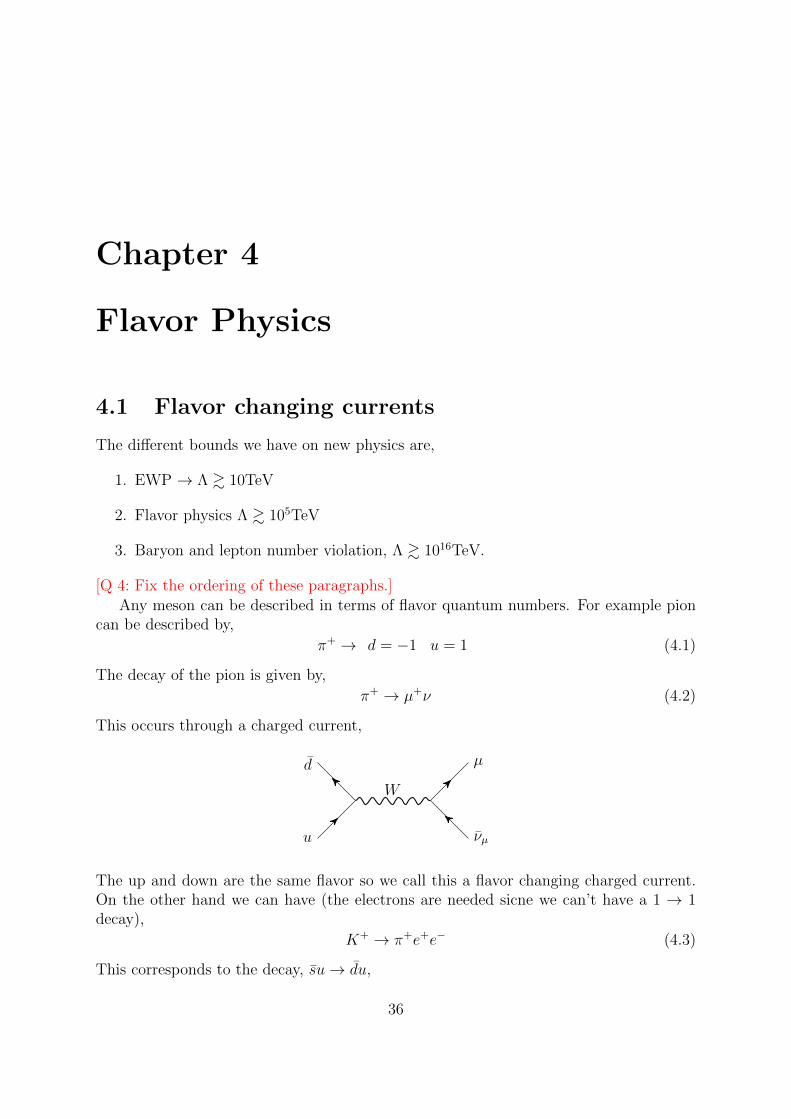
The decay of the pion is given by,
π+ → µ+ν (4.2)
This occurs through a charged current,
u
d
W
µ
νµ
The up and down are the same flavor so we call this a flavor changing charged current.On the other hand we can have (the electrons are needed sicne we can’t have a 1 → 1decay),
K+ → π+e+e− (4.3)
This corresponds to the decay, su→ du,
36
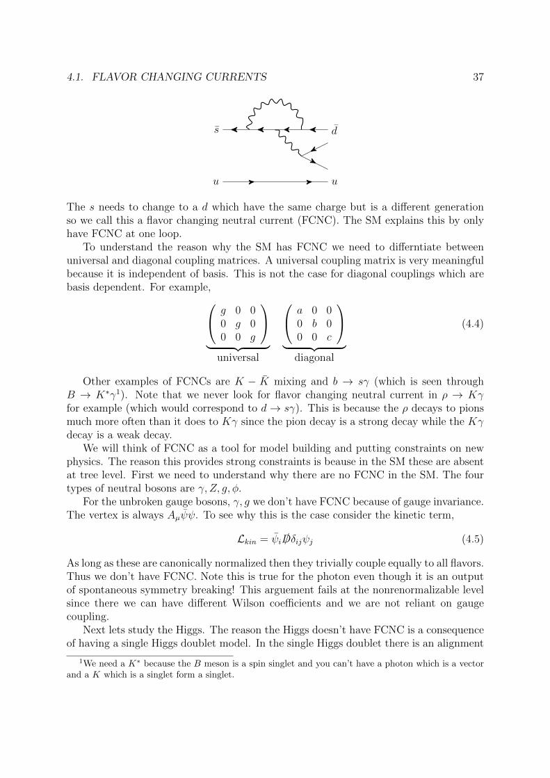
4.1. FLAVOR CHANGING CURRENTS 37
u u
s d
The s needs to change to a d which have the same charge but is a different generationso we call this a flavor changing neutral current (FCNC). The SM explains this by onlyhave FCNC at one loop.
To understand the reason why the SM has FCNC we need to differntiate betweenuniversal and diagonal coupling matrices. A universal coupling matrix is very meaningfulbecause it is independent of basis. This is not the case for diagonal couplings which arebasis dependent. For example, g 0 0
0 g 00 0 g
︸ ︷︷ ︸
universal
a 0 00 b 00 0 c
︸ ︷︷ ︸
diagonal
(4.4)
Other examples of FCNCs are K − K mixing and b → sγ (which is seen throughB → K∗γ1). Note that we never look for flavor changing neutral current in ρ → Kγfor example (which would correspond to d→ sγ). This is because the ρ decays to pionsmuch more often than it does to Kγ since the pion decay is a strong decay while the Kγdecay is a weak decay.
We will think of FCNC as a tool for model building and putting constraints on newphysics. The reason this provides strong constraints is beause in the SM these are absentat tree level. First we need to understand why there are no FCNC in the SM. The fourtypes of neutral bosons are γ, Z, g, φ.
For the unbroken gauge bosons, γ, g we don’t have FCNC because of gauge invariance.The vertex is always Aµψψ. To see why this is the case consider the kinetic term,
Lkin = ψi /Dδijψj (4.5)
As long as these are canonically normalized then they trivially couple equally to all flavors.Thus we don’t have FCNC. Note this is true for the photon even though it is an outputof spontaneous symmetry breaking! This arguement fails at the nonrenormalizable levelsince there we can have different Wilson coefficients and we are not reliant on gaugecoupling.
Next lets study the Higgs. The reason the Higgs doesn’t have FCNC is a consequenceof having a single Higgs doublet model. In the single Higgs doublet there is an alignment
1We need a K∗ because the B meson is a spin singlet and you can’t have a photon which is a vectorand a K which is a singlet form a singlet.
38 CHAPTER 4. FLAVOR PHYSICS
between the mass matrix and the Higgs couplings. As an example consider the downYukawas,
Y QLφDR → Y dL(φ+ v)dR (4.6)
The mass of the down-type quarks is,
m = Y v (4.7)
where Y is a matrix. When we diagonalize the mass matrix, the Yukawas are alsoautomatically diagonalized. Therefore there are no flavor changing contributions.
Now suppose we have two Higgs,
(Y1H1 + Y2H2)QLDR (4.8)
The masses are given by,
m = Y1v1 + Y2v2 (4.9)
while the matrix couplings to the down type quarks are Y1 and Y2 for h1 and h2 respec-tively. If the matrix U diagonalizes m then we have,
Lyuk = QLU†(Y1H1 + Y2H2)UDR (4.10)
but U †Y1U 6= Y diag1 since here the U ’s diagonalize the sum of Y1v1 and Y2v2 instead of
a single one. So diagonalizing the mass matrix doesn’t lead to diagonalization of theYukawas and hence we have FCNC in the Yukawa interactions. This is often not an issuebecause of the necessarily small couplings of the Higgs to the fermions.
Finally lets consider the Z boson. We write the Z coupling in the interaction basisand then move to the mass masis. For example we have,
uL/R → V uL/RuL/R (4.11)
dL/R → V dL/RdL/R (4.12)
We have four rotations to do. The W interaction we have,
LW = iuL /WdL → iuLVµL V
d†L/WdL (4.13)
and we define,
VCKM ≡ V uL V
d†L (4.14)
Now lets consider what happens in the neutral current sector. In this case we have,
LZ = iu /ZQZu→ iuV uQZVu† /Zu (4.15)
The “CKM-like” matrix is just the identity. To see why this happened lets recall the Zcharge,
QZ = T3 − q sin2 θw (4.16)
4.1. FLAVOR CHANGING CURRENTS 39
In general we can have some matrix,
QiZψ
iψi (4.17)
(we don’t need to necessarily impose flavor universality because the symmetry is sponta-neously broken regardless). We have,
QijZ =
Q1Z 0 0
0 Q2Z
...... ...
. . .
⇒ LZ = ψiQijψj (4.18)
where i, j are flavor indices. If QZ is universal then the Lagrangian is invariant underthe rotations that diagonalize the fermions. However, if this is not universal (but onlydiagonal) then,
V QZV† 6= diagonal matrix (4.19)
The condition for particles to mix is that they be under the same representation underall symmetries of the lorentz group. In the SM it just so happens that every field thathas the same quantum numbers (QN) under SU(2) × U(1)Y has the same QN underelectromagnetism. However, this is very unique to the SM. [Q 5: Why exactly does thishappen?] This results in universal couplings also for the Z boson.
Its easy to cook up a model which doesn’t have this property. Lets consider the 1generation SM and consider the vector-like quark (that the left and right have the samerepresentation),
ψL(3, 1)−1/3 ψR(3, 1)−1/3 QL(3, 2)1/6 dR(3, 1)−2/3 (4.20)
We have mass terms,
m1ψLψR +m2ψLdR + Y1vQLψR + Y2vQLdR (4.21)
The mass matrix is, (m1 m2
Y1v Y2v
)(4.22)
In principle we have four couplings of the Z and we want to see whether they are diagonal.We still have,
QZ = T3 − q sin2 θw (4.23)
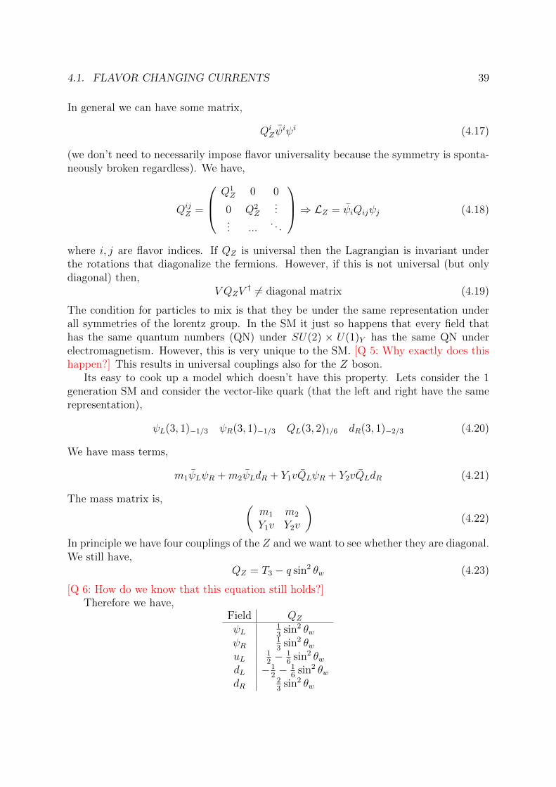
[Q 6: How do we know that this equation still holds?]Therefore we have,
Field QZ
ψL13
sin2 θwψR
13
sin2 θwuL
12− 1
6sin2 θw
dL −12− 1
6sin2 θw
dR23
sin2 θw
40 CHAPTER 4. FLAVOR PHYSICS
Therefore we have the down type quark matrices,
QLZ =
(12
sin2 θw 0
0 −12− sin2 θw
2
)(4.24)
QRZ =
(13
sin2 θw 00 1
3sin2 θw
)(4.25)
Since the QLZ charge is not universal we would expect FCNC in the left sector.
The way the SM deals with the requirement of no FCNC is to make all the fermionscopies of one another.
Now suppose we have a neutral heavy gauge boson that is not the Z boson (Z ′). ThisZ ′ can be problematic because it can mediate FCNC. In order for this new boson not tocreate FCNC, we must require that all the SM fermions be under the same representationof this new boson.
Lets now consider the coupling of the W in this model, the CKM matrix. For the Wcoupling we have,
uLVu†
L V dLdL (4.26)
The V uL is still a 3 × 3 matrix, but V d
L is not a 4 × 4 matrix projected out to the statesthat interact with the W . The CKM is no longer a unitary matrix. In this kind of modelswhere we get FCNC we also get nonunitarity in the CKM.
4.1.1 Unitarity triangles
The unitarity of the CKM says that,∑k
VikV∗jk = 0 (4.27)
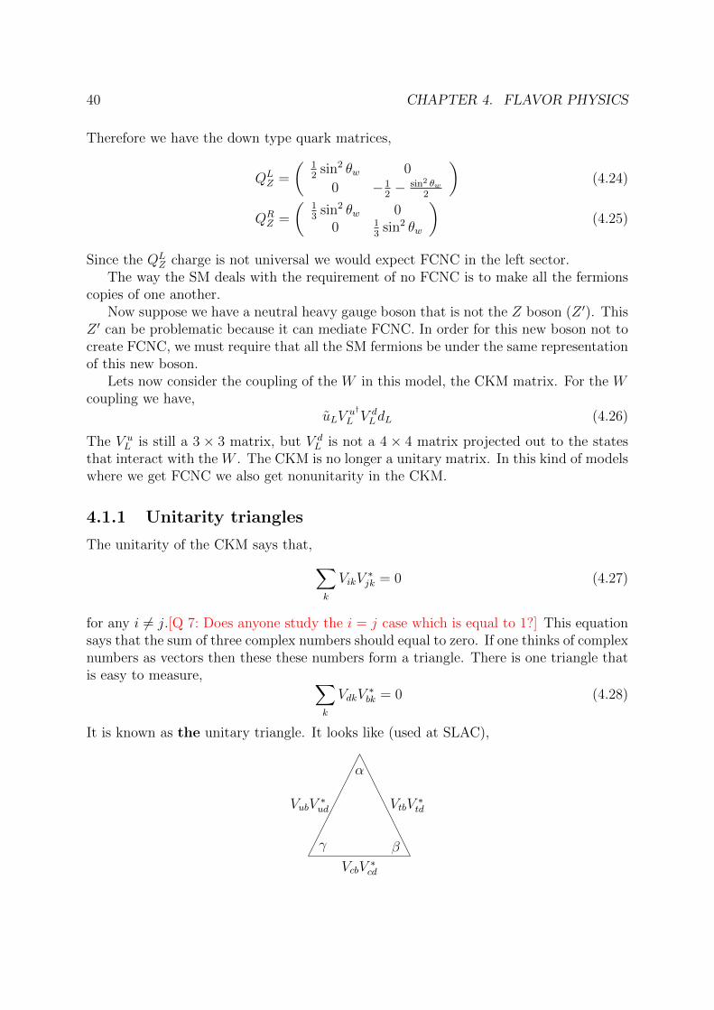
for any i 6= j.[Q 7: Does anyone study the i = j case which is equal to 1?] This equationsays that the sum of three complex numbers should equal to zero. If one thinks of complexnumbers as vectors then these these numbers form a triangle. There is one triangle thatis easy to measure, ∑
k
VdkV∗bk = 0 (4.28)
It is known as the unitary triangle. It looks like (used at SLAC),
VcbV∗cd
VtbV∗tdVubV
∗ud
γ β
α
4.2. FCNC AT 1 LOOP 41
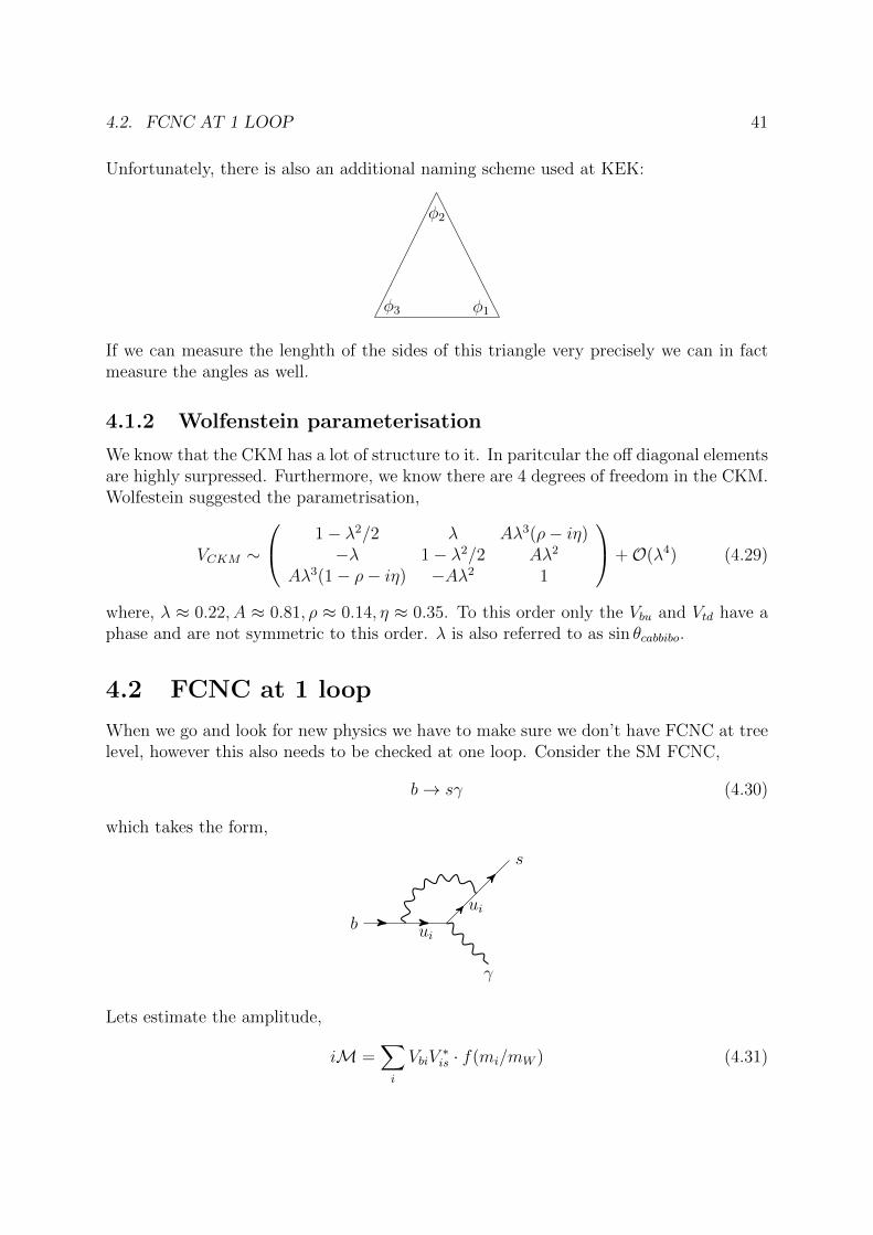
Unfortunately, there is also an additional naming scheme used at KEK:
φ3 φ1
φ2
If we can measure the lenghth of the sides of this triangle very precisely we can in factmeasure the angles as well.
4.1.2 Wolfenstein parameterisation
We know that the CKM has a lot of structure to it. In paritcular the off diagonal elementsare highly surpressed. Furthermore, we know there are 4 degrees of freedom in the CKM.Wolfestein suggested the parametrisation,
VCKM ∼
1− λ2/2 λ Aλ3(ρ− iη)−λ 1− λ2/2 Aλ2
Aλ3(1− ρ− iη) −Aλ2 1
+O(λ4) (4.29)
where, λ ≈ 0.22, A ≈ 0.81, ρ ≈ 0.14, η ≈ 0.35. To this order only the Vbu and Vtd have aphase and are not symmetric to this order. λ is also referred to as sin θcabbibo.
4.2 FCNC at 1 loop
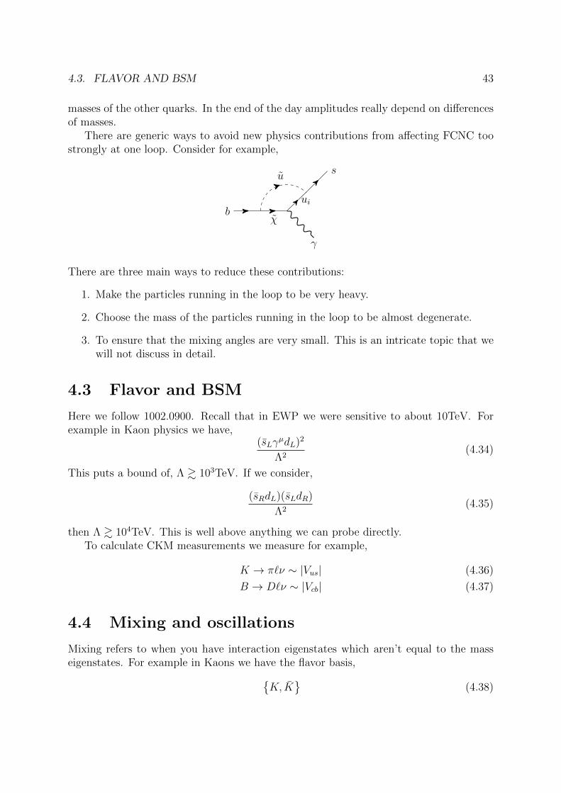
When we go and look for new physics we have to make sure we don’t have FCNC at treelevel, however this also needs to be checked at one loop. Consider the SM FCNC,
b→ sγ (4.30)
which takes the form,
b ui
ui
s
γ
Lets estimate the amplitude,
iM =∑i
VbiV∗is · f(mi/mW ) (4.31)

42 CHAPTER 4. FLAVOR PHYSICS
where we ignore the dependence on the masses of the external particles, which are inprinciple important but because we will in the end take the internal particle to be thetop these will be a higher order effect.
Note that if f(...) was equal to 1 the amplitude would be zero! due to unitarity of theCKM. We can write f as a Taylor expansion2,
f
(m2i
m2W
)= f0 + f2
m2i
m2W
+ f4m4i
m4W
+ ... (4.32)
Note that f0 is unphysical. This is because the CKM gaurentees this term is zero. Thisis very important because f0 is where the logarithmic divergence would live. Since thereare no FCNC, there is no counterterm for this process. In fact QFT tells us that thelowest order contribution must be finite, which in this case is the one loop contribution.
Note that if we consider the model above and a process with a Z:
b ui
ui
s
Z
Since the CKM is not unitary, this diagram can diverge. However, here we also haveFCNC at tree level and hence we have a counterterm.
Now lets return to the case of a unitary CKM matrix. The amplitude is already smallsince it occurs at one loop. However, if we assume mi is small we can write,
f
(m2i
m2W
)≈ f0 + f2
(m2i
m2W
)(4.33)
If the CKM is unitary we can forget about f0 and we have quadratic dependence on theheavy field, m2
t . This is essentially the GIM mechanism [Q 8: expand on this.] While thisis not really relevant here since mt > mW however it is used for K → µ+µ− for example.
Notice that this is counterintiutive because the heavier the massive field, the moreimportant it becomes. The decoupling theorem, that says that the heavier the field theless important it should be, is failing. The reason is happening because of the Higgs.What’s really growing is not the mass of the top but the Yukawa couplings to the Higgs.So you can’t really take the mass to infinity because then the theory becomes then thecoupling becomes too large and the theory is nonperturbative.
Now suppose that quarks were all degenerate. If all the quarks were degerate thenthe mass can be taken out of the sum and the amplitude would again vanish by unitarityof the CKM. Therefore, we don’t really have just the mass of the top, but also the small
2This expansion is not really justified for the top but lets ignore this caveat for now.
4.3. FLAVOR AND BSM 43
masses of the other quarks. In the end of the day amplitudes really depend on differencesof masses.
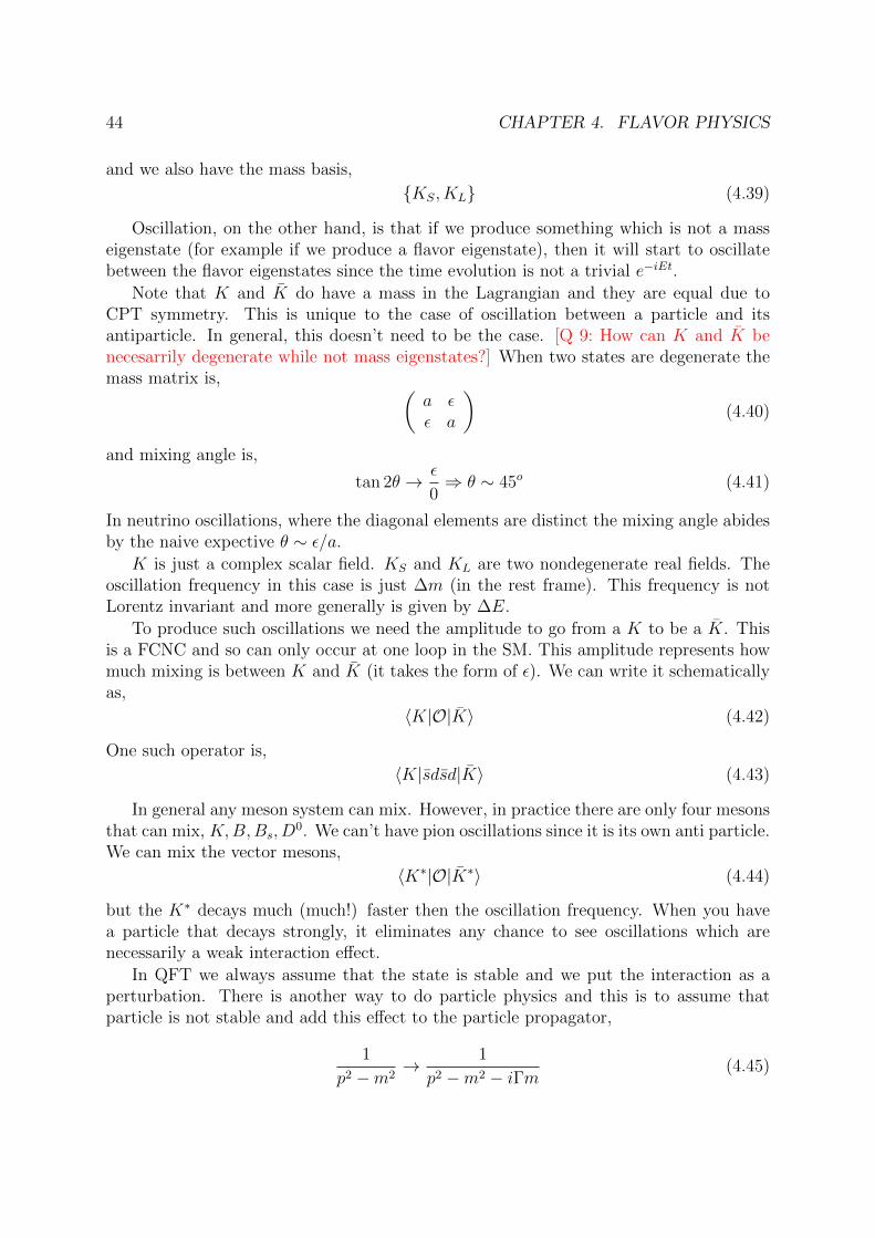
There are generic ways to avoid new physics contributions from affecting FCNC toostrongly at one loop. Consider for example,
bχ
ui
s
γ
u
There are three main ways to reduce these contributions:
1. Make the particles running in the loop to be very heavy.
2. Choose the mass of the particles running in the loop to be almost degenerate.
3. To ensure that the mixing angles are very small. This is an intricate topic that wewill not discuss in detail.
4.3 Flavor and BSM
Here we follow 1002.0900. Recall that in EWP we were sensitive to about 10TeV. Forexample in Kaon physics we have,
(sLγµdL)2
Λ2(4.34)
This puts a bound of, Λ & 103TeV. If we consider,
(sRdL)(sLdR)
Λ2(4.35)
then Λ & 104TeV. This is well above anything we can probe directly.To calculate CKM measurements we measure for example,
K → π`ν ∼ |Vus| (4.36)
B → D`ν ∼ |Vcb| (4.37)
4.4 Mixing and oscillations
Mixing refers to when you have interaction eigenstates which aren’t equal to the masseigenstates. For example in Kaons we have the flavor basis,
K, K
(4.38)
44 CHAPTER 4. FLAVOR PHYSICS
and we also have the mass basis,
KS, KL (4.39)
Oscillation, on the other hand, is that if we produce something which is not a masseigenstate (for example if we produce a flavor eigenstate), then it will start to oscillatebetween the flavor eigenstates since the time evolution is not a trivial e−iEt.
Note that K and K do have a mass in the Lagrangian and they are equal due toCPT symmetry. This is unique to the case of oscillation between a particle and itsantiparticle. In general, this doesn’t need to be the case. [Q 9: How can K and K benecesarrily degenerate while not mass eigenstates?] When two states are degenerate themass matrix is, (
a εε a
)(4.40)
and mixing angle is,
tan 2θ → ε
0⇒ θ ∼ 45o (4.41)
In neutrino oscillations, where the diagonal elements are distinct the mixing angle abidesby the naive expective θ ∼ ε/a.
K is just a complex scalar field. KS and KL are two nondegenerate real fields. Theoscillation frequency in this case is just ∆m (in the rest frame). This frequency is notLorentz invariant and more generally is given by ∆E.
To produce such oscillations we need the amplitude to go from a K to be a K. Thisis a FCNC and so can only occur at one loop in the SM. This amplitude represents howmuch mixing is between K and K (it takes the form of ε). We can write it schematicallyas,
〈K|O|K〉 (4.42)
One such operator is,
〈K|sdsd|K〉 (4.43)
In general any meson system can mix. However, in practice there are only four mesonsthat can mix, K,B,Bs, D
0. We can’t have pion oscillations since it is its own anti particle.We can mix the vector mesons,
〈K∗|O|K∗〉 (4.44)
but the K∗ decays much (much!) faster then the oscillation frequency. When you havea particle that decays strongly, it eliminates any chance to see oscillations which arenecessarily a weak interaction effect.
In QFT we always assume that the state is stable and we put the interaction as aperturbation. There is another way to do particle physics and this is to assume thatparticle is not stable and add this effect to the particle propagator,
1
p2 −m2→ 1
p2 −m2 − iΓm(4.45)
4.4. MIXING AND OSCILLATIONS 45
The original propagator is unitary, however this is not true for the decaying propagator.This requires a nonhermitian Hamiltonian,
H = M − i
2Γ (4.46)
where M and Γ are hermitian (any nonhermitian Hamiltonian can be written as a sumof hermitian and antihermitian parts). We write,
H2×2 =
[ K K
K H11 H12
K H21 H22
](4.47)
Lets discuss each term one by one. H22 is equal to H11 by CPT and M12 = M∗21,Γ12 = Γ∗21.
[Q 10: Check this statement].M11 = mK ,Γ11 = ΓK . This is the mass and width of the Kaon if there were no mixing.
M12 is related to the matrix element that we wrote above. Any matrix element can bewritten in terms of its real and imaginary parts. The real part contributes to the massand the imaginary corresponds to decay.
M12 ∼ Res 〈K|O|K〉 (4.48)
Γ12 ∼ Ims 〈K|O|K〉 (4.49)
where here we take the real and imaginary parts of what we call strong phase. In generalwe like to distinguish between two kinds of phases, CP-even phase (“strong phase”) andCP-odd phase (“weak phase”). A CP-even phase is one that does not change under CP.CP-odd phases arise from phases in the Lagrangian. A strong phase is typically due totime evolution. The phase due to time evoluation doesn’t change under CP. The i in theHamiltonian is a strong phase. If we have same electron with wavefunction, ψ, evolvingin time,
ψ(t) = e−iHtψ(0) (4.50)
If we have a positron it propagates with the same e−iHt (there is no i→ −i here).Typically in QFT we just diagonalize the mass matrix, as oppose to the Hamiltonian.
This is an approximation. The eigenvalues are,
µα = Mα −i
2Γα (4.51)
where α = 1, 2. Note that Mα and Γα are not the eigenvalues of the mass and decaymatrices.
We write the mass eigenstates as,
KL = p |K〉+ q |K〉 (4.52)
KS = p |K〉 − q |K〉 (4.53)
such that p2 + q2 = 1.
46 CHAPTER 4. FLAVOR PHYSICS
Note that this rotation is not unitary. This results in,
〈KS|KL〉 = |p|2 − |q|2 (4.54)
This means that you can produce a KS but if you measure it afterwords you can measurea KL.
Furthermore, one can show that if
arg (M12Γ∗12) = 0 (4.55)
then|q| = |p| (4.56)
[Q 11: Check]If CP is a good symmetry then,
[H,CP ] = 0 (4.57)
If we have a nondegenerate state then the state must be an eigenstate of all the symmetriesthat commute with the Hamiltonian. Since KL and KS are nondegenerate then if CPcommutes with Hamiltonian then we can choose,
CP (KS) =1√2CP (K + K) = +KS (4.58)
CP (KL) =1√2CP (K − K) = −KL (4.59)
We have seen that KL can decay into 2π (which are CP even). Thus we know that theweak interaction has /CP.We now define the eigenvalues,
µα = Mα −i
2Γα (4.60)
which gives,
∆m = m1 −m2 (4.61)
∆Γ = Γ1 − Γ2 (4.62)
in the limit of CP we have,
∆m = 2 |M12| (4.63)
∆Γ = 2 |Γ12| (4.64)
We define,
x ≡ δm
Γy ≡ ∆Γ
2Γ(4.65)
andθ = arg (M12Γ∗12) (4.66)
4.4. MIXING AND OSCILLATIONS 47
We now assume CP conservation,
KL,S =1√2
(K ± K
)(4.67)
We define K(t) as the state at time t for a state that started out as a K.
K(t) = cos∆mt
2|K〉+ i sin
∆mt
2K (4.68)
The probability for measuring a K at time t is3
P (K → K) [t] =1 + cos ∆mt
2(4.69)
P (K → K) =1− cos ∆mt
2(4.70)
One can use this to measure ∆m. Here we have ignored the decay amplitude. We wereable to do this because of timescales. The relevant time scale in this problem is ∆m.
Consider the case that x 1. In this case the meson will decay very quickly and thereis no time for things to oscillate. Now suppose that ∆x 1, in this case the oscillationis extremely fast and the probability averages to 1/2. Oscillatons are important if x ∼ 1.Experimentally it has been found that
xK ∼ 1
xB ∼ 1
xD ∼ 10−2
xBs ∼ 25
The fact that xK and xB are so close to 1 is accidental finetuning.Lets now return to the braket we mentioned above,
M12 = Re 〈k|O|k〉 (4.71)
O needs to be a ∆s = 2 operator - sdsd. Recall that a s field annihilates a free |s〉 stateand creates a free |s〉, and similarly for the d field. But suddenly we are asking our fieldsto act upon a bounded |s〉 and a bounded |d〉. We need to specify how our fields act onthe bound state. To calculate this braket we need lattice QCD.
The diagram is,
sui
s
d ujd∼ g4 sdsd
M2W
×∑ij
VidV∗isVjdV
∗is × F (xi, xj)
3In practice we can differentiate between a K and K by its decay products since one decays with anelectron and another with an electron.
48 CHAPTER 4. FLAVOR PHYSICS
where F is a finite function and xi ≡ m2i
m2W
. Here we see the GIM mechanism taking place
because if we had no mass dependence in F then the diagram would be zero. Anotherinteresting point is that this amplitude is g4. We say this is second order in the weakinteraction. [Q 12: Didn’t we just say above that we can’t calculate it because of QCD?How do you relate this calculation to the above?] In an explicit calculation one can showthat,
F ∼ xi ∼m2c
m2W
(4.72)
where we only keep the charm due to CKM suppression. This calculation is only validif none of the interactions in the loop are of O(ΛQCD). For the B quark this is a goodassumption, however this is not the case in Kaon or charm physics. Therefore the calcu-lation only holds up to order 1 corrections.
4.5 CP Violation
CP violation is a strong constraint on new physics. [Q 13: Show why complex numbersand CPV are related.] Fundamentally, /CP and flavor are two distinct phenomena, butin the SM they seem to come together. We build the SM such that we only have 1 /CPphase. The only other phase in the SM is θQCD.
In general if we have some process which takes us from A→ B then,
P (A→ B)(x) 6= P (A→ B)(−x)⇒ /P (4.73)
P (A+ → B+) 6= P (A− → B−)⇒ /C (4.74)
P (A→ B) 6= P (B → A) ⇒ /T (4.75)
P (A→ B) 6= P (A→ B) ⇒ /CP (4.76)
P (A→ B) 6= P (B → A) ⇒ /CPT (4.77)
where we use the common notation that the bar over the states, A and B, is bothconjugation and reversal of x→ −x.
In 1964 people found KL → ππ. This was a huge surprise because people knew thatKS decayed to ππ and if CP is a good quantum number then both couldn’t decay to ππ.KL decays to ππ about 10−3 of the time. In 1967 people found,
Γ(KL → π−e+ν
)6= Γ
(KL → π+e−ν
)(4.78)
Until this point there was no unambigious definition of the electron. After this experimentyou can define the electron to be the outgoing particle that corresponds to the longerlifetime KL decay.
In 1973 the third generation was predicted since it was needed for /CP. In 1990’s theyfound that KL → π+π− 6= KL → π0π0 [Q 14: What is the significance of this result?]
To know that KL → ππ is CP violating note the following. A symmetry is an operatorthat commutes with the Hamiltonian, [O, H] = 0. Furthermore, for all non degenerate
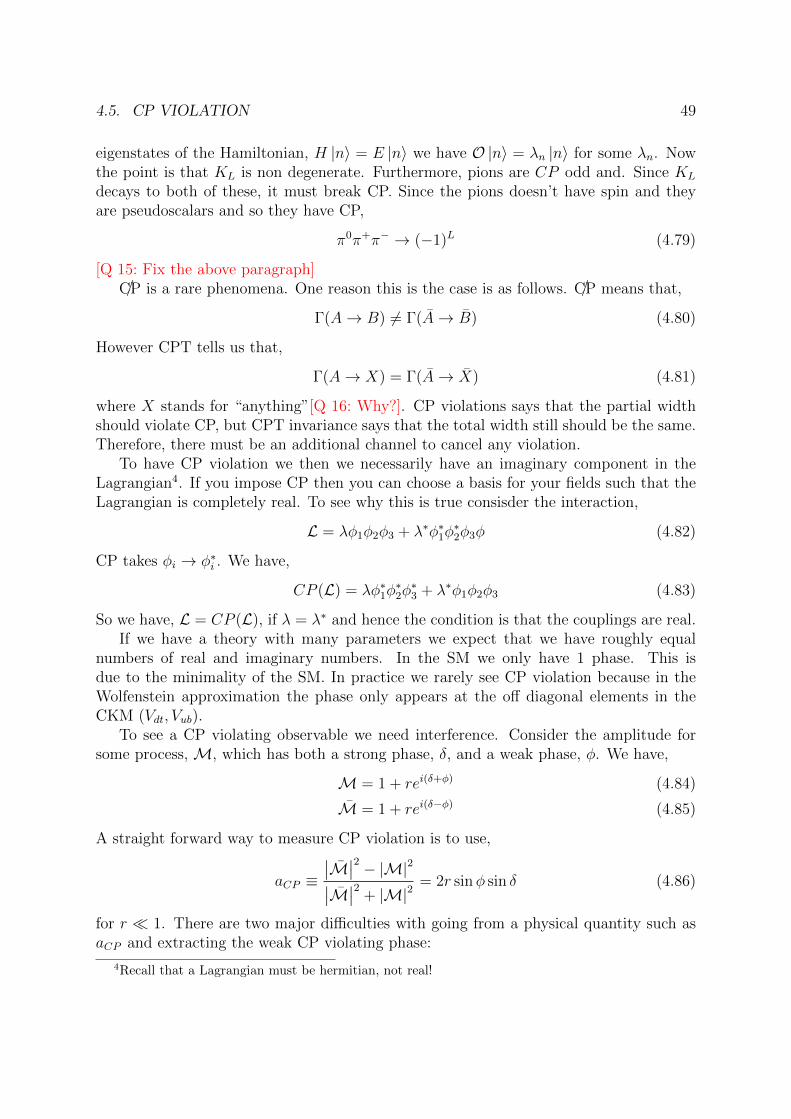
4.5. CP VIOLATION 49
eigenstates of the Hamiltonian, H |n〉 = E |n〉 we have O |n〉 = λn |n〉 for some λn. Nowthe point is that KL is non degenerate. Furthermore, pions are CP odd and. Since KL
decays to both of these, it must break CP. Since the pions doesn’t have spin and theyare pseudoscalars and so they have CP,
π0π+π− → (−1)L (4.79)
[Q 15: Fix the above paragraph]/CP is a rare phenomena. One reason this is the case is as follows. /CP means that,
Γ(A→ B) 6= Γ(A→ B) (4.80)
However CPT tells us that,
Γ(A→ X) = Γ(A→ X) (4.81)
where X stands for “anything”[Q 16: Why?]. CP violations says that the partial widthshould violate CP, but CPT invariance says that the total width still should be the same.Therefore, there must be an additional channel to cancel any violation.
To have CP violation we then we necessarily have an imaginary component in theLagrangian4. If you impose CP then you can choose a basis for your fields such that theLagrangian is completely real. To see why this is true consisder the interaction,
L = λφ1φ2φ3 + λ∗φ∗1φ∗2φ3φ (4.82)
CP takes φi → φ∗i . We have,
CP (L) = λφ∗1φ∗2φ∗3 + λ∗φ1φ2φ3 (4.83)
So we have, L = CP (L), if λ = λ∗ and hence the condition is that the couplings are real.If we have a theory with many parameters we expect that we have roughly equal
numbers of real and imaginary numbers. In the SM we only have 1 phase. This isdue to the minimality of the SM. In practice we rarely see CP violation because in theWolfenstein approximation the phase only appears at the off diagonal elements in theCKM (Vdt, Vub).
To see a CP violating observable we need interference. Consider the amplitude forsome process, M, which has both a strong phase, δ, and a weak phase, φ. We have,
M = 1 + rei(δ+φ) (4.84)
M = 1 + rei(δ−φ) (4.85)
A straight forward way to measure CP violation is to use,
aCP ≡∣∣M∣∣2 − |M|2∣∣M∣∣2 + |M|2
= 2r sinφ sin δ (4.86)
for r 1. There are two major difficulties with going from a physical quantity such asaCP and extracting the weak CP violating phase:
4Recall that a Lagrangian must be hermitian, not real!
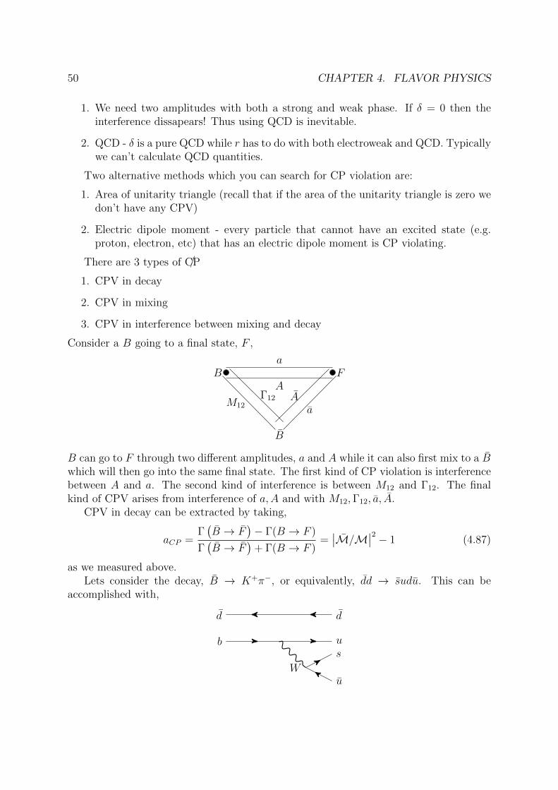
50 CHAPTER 4. FLAVOR PHYSICS
1. We need two amplitudes with both a strong and weak phase. If δ = 0 then theinterference dissapears! Thus using QCD is inevitable.
2. QCD - δ is a pure QCD while r has to do with both electroweak and QCD. Typicallywe can’t calculate QCD quantities.
Two alternative methods which you can search for CP violation are:
1. Area of unitarity triangle (recall that if the area of the unitarity triangle is zero wedon’t have any CPV)
2. Electric dipole moment - every particle that cannot have an excited state (e.g.proton, electron, etc) that has an electric dipole moment is CP violating.
There are 3 types of /CP
1. CPV in decay
2. CPV in mixing
3. CPV in interference between mixing and decay
Consider a B going to a final state, F ,
BA
Fa
B
Aa
M12Γ12
B can go to F through two different amplitudes, a and A while it can also first mix to a Bwhich will then go into the same final state. The first kind of CP violation is interferencebetween A and a. The second kind of interference is between M12 and Γ12. The finalkind of CPV arises from interference of a,A and with M12,Γ12, a, A.
CPV in decay can be extracted by taking,
aCP =Γ(B → F
)− Γ(B → F )
Γ(B → F
)+ Γ(B → F )
=∣∣M/M
∣∣2 − 1 (4.87)
as we measured above.Lets consider the decay, B → K+π−, or equivalently, dd → sudu. This can be
accomplished with,
d d
b u
W
s
u
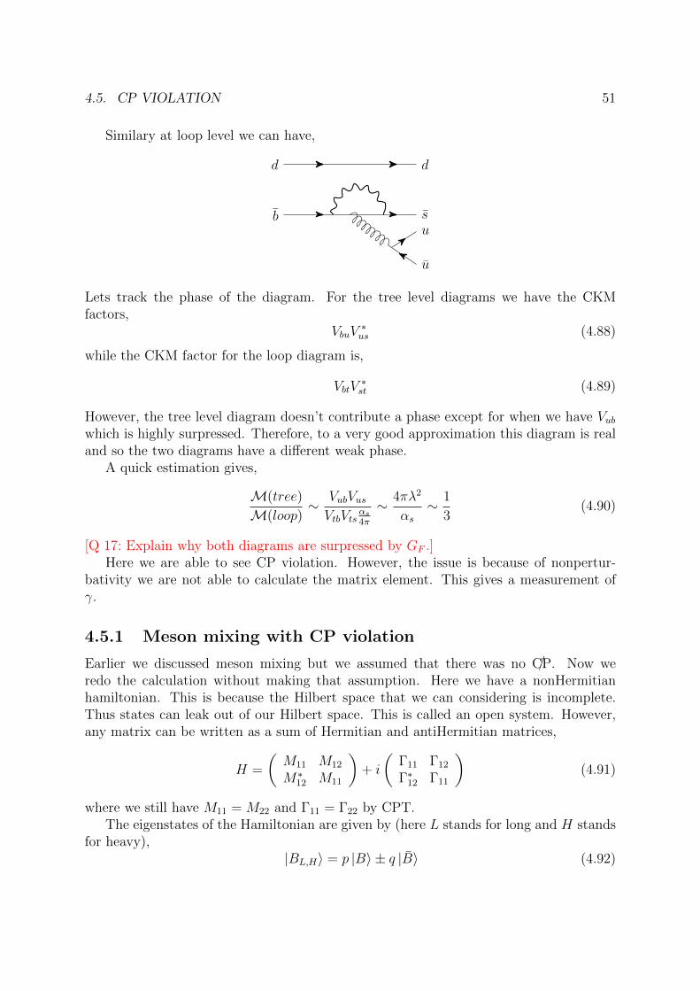
4.5. CP VIOLATION 51
Similary at loop level we can have,
d d
b su
u
Lets track the phase of the diagram. For the tree level diagrams we have the CKMfactors,
VbuV∗us (4.88)
while the CKM factor for the loop diagram is,
VbtV∗st (4.89)
However, the tree level diagram doesn’t contribute a phase except for when we have Vubwhich is highly surpressed. Therefore, to a very good approximation this diagram is realand so the two diagrams have a different weak phase.
A quick estimation gives,
M(tree)
M(loop)∼ VubVusVtbVts
αs4π
∼ 4πλ2
αs∼ 1
3(4.90)
[Q 17: Explain why both diagrams are surpressed by GF .]Here we are able to see CP violation. However, the issue is because of nonpertur-
bativity we are not able to calculate the matrix element. This gives a measurement ofγ.
4.5.1 Meson mixing with CP violation
Earlier we discussed meson mixing but we assumed that there was no /CP. Now weredo the calculation without making that assumption. Here we have a nonHermitianhamiltonian. This is because the Hilbert space that we can considering is incomplete.Thus states can leak out of our Hilbert space. This is called an open system. However,any matrix can be written as a sum of Hermitian and antiHermitian matrices,
H =
(M11 M12
M∗12 M11
)+ i
(Γ11 Γ12
Γ∗12 Γ11
)(4.91)
where we still have M11 = M22 and Γ11 = Γ22 by CPT.The eigenstates of the Hamiltonian are given by (here L stands for long and H stands
for heavy),|BL,H〉 = p |B〉 ± q |B〉 (4.92)
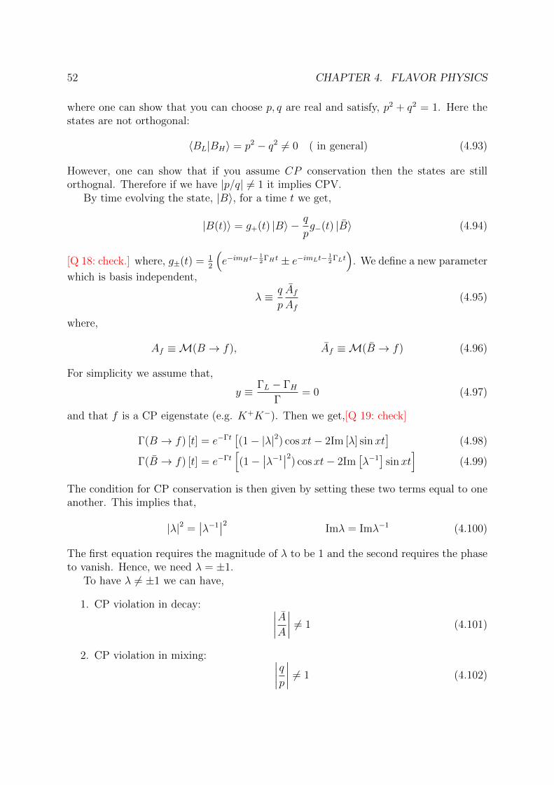
52 CHAPTER 4. FLAVOR PHYSICS
where one can show that you can choose p, q are real and satisfy, p2 + q2 = 1. Here thestates are not orthogonal:
〈BL|BH〉 = p2 − q2 6= 0 ( in general) (4.93)
However, one can show that if you assume CP conservation then the states are stillorthognal. Therefore if we have |p/q| 6= 1 it implies CPV.
By time evolving the state, |B〉, for a time t we get,
|B(t)〉 = g+(t) |B〉 − q
pg−(t) |B〉 (4.94)
[Q 18: check.] where, g±(t) = 12
(e−imH t−
12
ΓH t ± e−imLt− 12
ΓLt)
. We define a new parameter
which is basis independent,
λ ≡ q
p
AfAf
(4.95)
where,
Af ≡M(B → f), Af ≡M(B → f) (4.96)
For simplicity we assume that,
y ≡ ΓL − ΓHΓ
= 0 (4.97)
and that f is a CP eigenstate (e.g. K+K−). Then we get,[Q 19: check]
Γ(B → f) [t] = e−Γt[(1− |λ|2) cosxt− 2Im [λ] sinxt
](4.98)
Γ(B → f) [t] = e−Γt[(1−
∣∣λ−1∣∣2) cosxt− 2Im
[λ−1]
sinxt]
(4.99)
The condition for CP conservation is then given by setting these two terms equal to oneanother. This implies that,
|λ|2 =∣∣λ−1
∣∣2 Imλ = Imλ−1 (4.100)
The first equation requires the magnitude of λ to be 1 and the second requires the phaseto vanish. Hence, we need λ = ±1.
To have λ 6= ±1 we can have,
1. CP violation in decay: ∣∣∣∣AA∣∣∣∣ 6= 1 (4.101)
2. CP violation in mixing: ∣∣∣∣qp∣∣∣∣ 6= 1 (4.102)
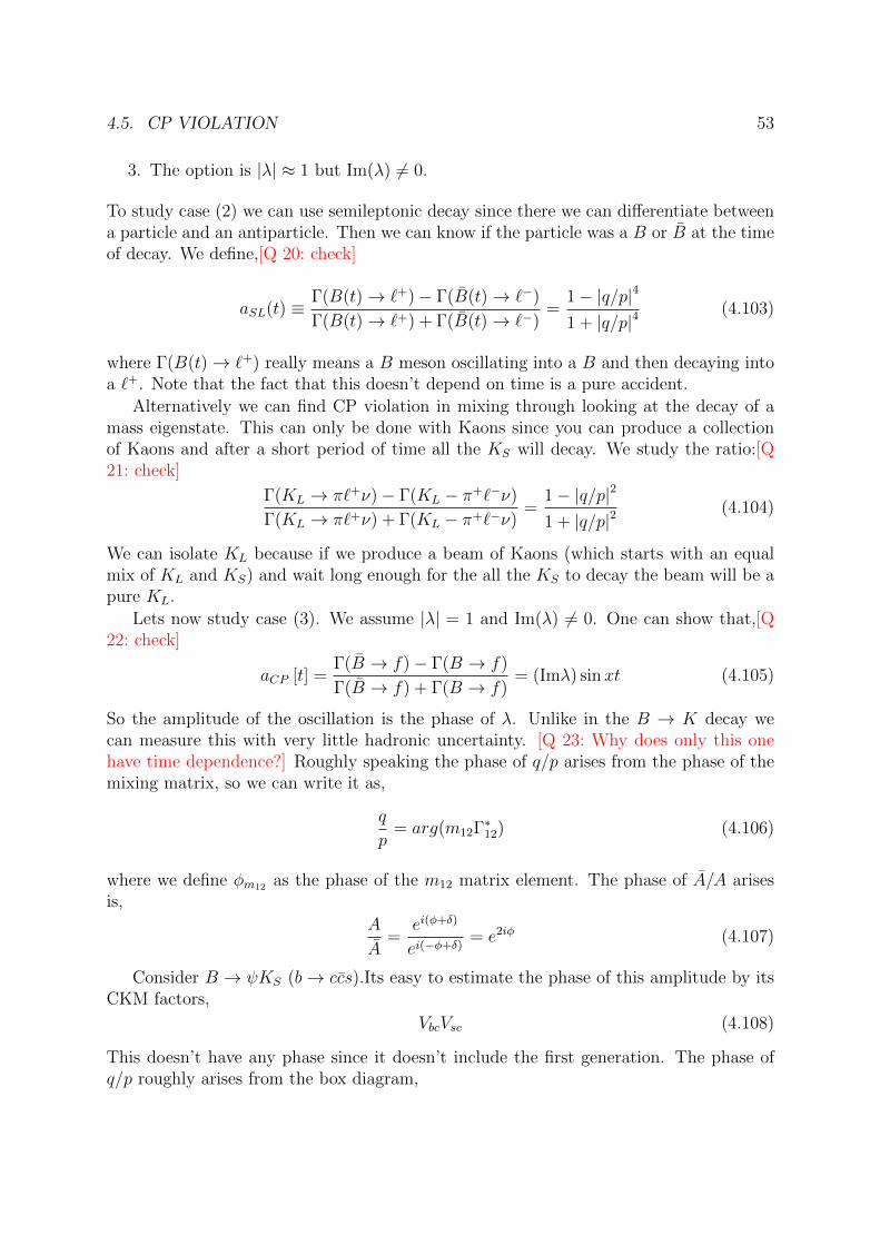
4.5. CP VIOLATION 53
3. The option is |λ| ≈ 1 but Im(λ) 6= 0.
To study case (2) we can use semileptonic decay since there we can differentiate betweena particle and an antiparticle. Then we can know if the particle was a B or B at the timeof decay. We define,[Q 20: check]
aSL(t) ≡ Γ(B(t)→ `+)− Γ(B(t)→ `−)
Γ(B(t)→ `+) + Γ(B(t)→ `−)=
1− |q/p|4
1 + |q/p|4(4.103)
where Γ(B(t)→ `+) really means a B meson oscillating into a B and then decaying intoa `+. Note that the fact that this doesn’t depend on time is a pure accident.
Alternatively we can find CP violation in mixing through looking at the decay of amass eigenstate. This can only be done with Kaons since you can produce a collectionof Kaons and after a short period of time all the KS will decay. We study the ratio:[Q21: check]
Γ(KL → π`+ν)− Γ(KL − π+`−ν)
Γ(KL → π`+ν) + Γ(KL − π+`−ν)=
1− |q/p|2
1 + |q/p|2(4.104)
We can isolate KL because if we produce a beam of Kaons (which starts with an equalmix of KL and KS) and wait long enough for the all the KS to decay the beam will be apure KL.
Lets now study case (3). We assume |λ| = 1 and Im(λ) 6= 0. One can show that,[Q22: check]
aCP [t] =Γ(B → f)− Γ(B → f)
Γ(B → f) + Γ(B → f)= (Imλ) sinxt (4.105)
So the amplitude of the oscillation is the phase of λ. Unlike in the B → K decay wecan measure this with very little hadronic uncertainty. [Q 23: Why does only this onehave time dependence?] Roughly speaking the phase of q/p arises from the phase of themixing matrix, so we can write it as,
q
p= arg(m12Γ∗12) (4.106)
where we define φm12 as the phase of the m12 matrix element. The phase of A/A arisesis,
A
A=
ei(φ+δ)
ei(−φ+δ)= e2iφ (4.107)
Consider B → ψKS (b→ ccs).Its easy to estimate the phase of this amplitude by itsCKM factors,
VbcVsc (4.108)
This doesn’t have any phase since it doesn’t include the first generation. The phase ofq/p roughly arises from the box diagram,
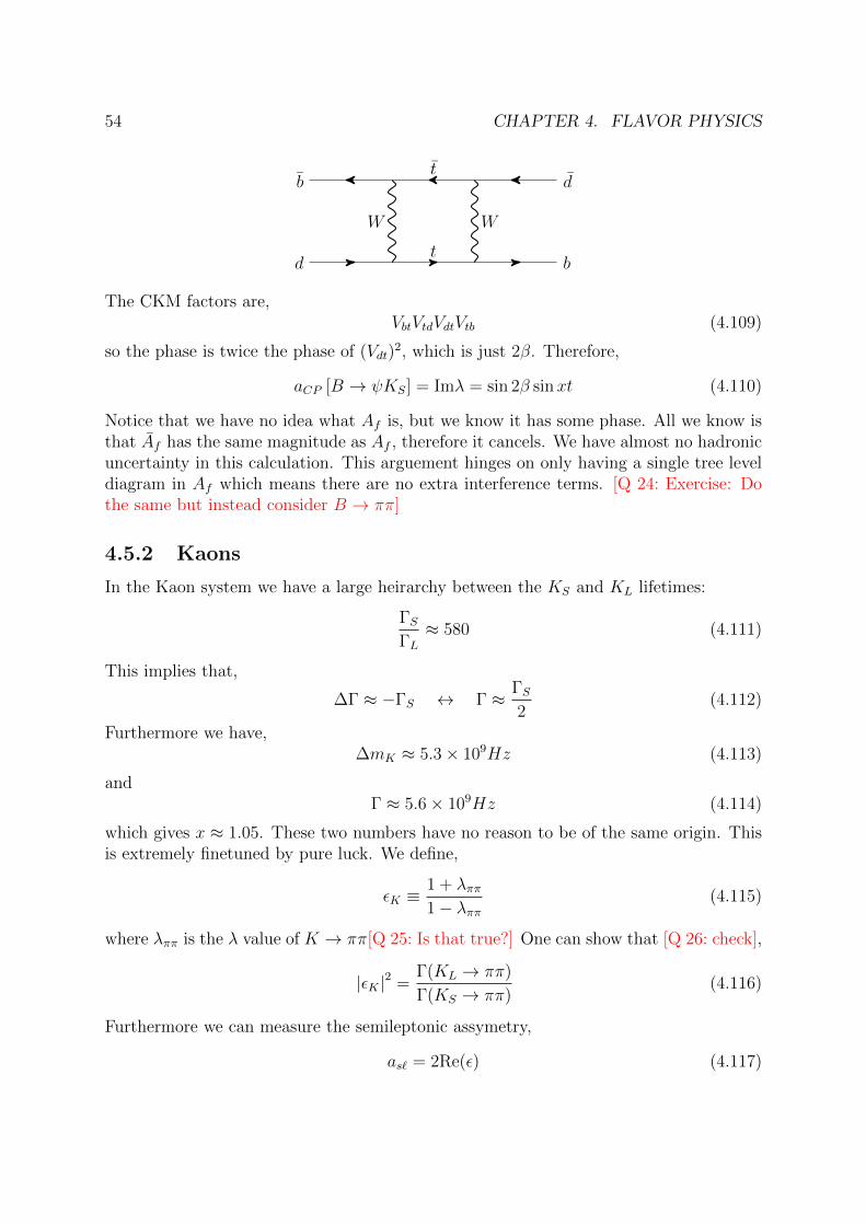
54 CHAPTER 4. FLAVOR PHYSICS
bt
d
dt
b
W W
The CKM factors are,VbtVtdVdtVtb (4.109)
so the phase is twice the phase of (Vdt)2, which is just 2β. Therefore,
aCP [B → ψKS] = Imλ = sin 2β sinxt (4.110)
Notice that we have no idea what Af is, but we know it has some phase. All we know isthat Af has the same magnitude as Af , therefore it cancels. We have almost no hadronicuncertainty in this calculation. This arguement hinges on only having a single tree leveldiagram in Af which means there are no extra interference terms. [Q 24: Exercise: Dothe same but instead consider B → ππ]
4.5.2 Kaons
In the Kaon system we have a large heirarchy between the KS and KL lifetimes:
ΓSΓL≈ 580 (4.111)
This implies that,
∆Γ ≈ −ΓS ↔ Γ ≈ ΓS2
(4.112)
Furthermore we have,∆mK ≈ 5.3× 10⁹Hz (4.113)
andΓ ≈ 5.6× 10⁹Hz (4.114)
which gives x ≈ 1.05. These two numbers have no reason to be of the same origin. Thisis extremely finetuned by pure luck. We define,
εK ≡1 + λππ1− λππ
(4.115)
where λππ is the λ value of K → ππ[Q 25: Is that true?] One can show that [Q 26: check],
|εK |2 =Γ(KL → ππ)
Γ(KS → ππ)(4.116)
Furthermore we can measure the semileptonic assymetry,
as` = 2Re(ε) (4.117)
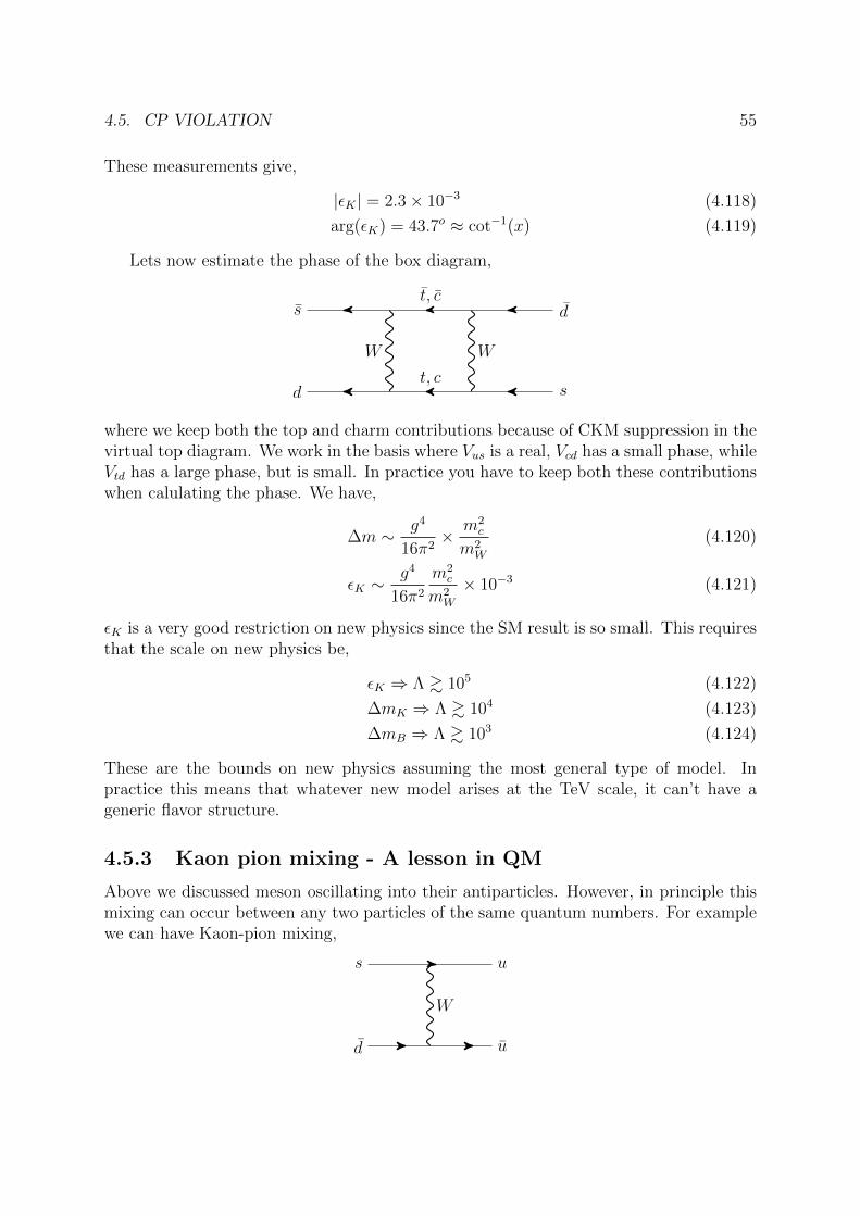
4.5. CP VIOLATION 55
These measurements give,
|εK | = 2.3× 10⁻³ (4.118)
arg(εK) = 43.7o ≈ cot−1(x) (4.119)
Lets now estimate the phase of the box diagram,
st, c
d
dt, c
s
W W
where we keep both the top and charm contributions because of CKM suppression in thevirtual top diagram. We work in the basis where Vus is a real, Vcd has a small phase, whileVtd has a large phase, but is small. In practice you have to keep both these contributionswhen calulating the phase. We have,
∆m ∼ g4
16π2× m2
c
m2W
(4.120)
εK ∼g4
16π2
m2c
m2W
× 10−3 (4.121)
εK is a very good restriction on new physics since the SM result is so small. This requiresthat the scale on new physics be,
εK ⇒ Λ & 105 (4.122)
∆mK ⇒ Λ & 104 (4.123)
∆mB ⇒ Λ & 103 (4.124)
These are the bounds on new physics assuming the most general type of model. Inpractice this means that whatever new model arises at the TeV scale, it can’t have ageneric flavor structure.
4.5.3 Kaon pion mixing - A lesson in QM
Above we discussed meson oscillating into their antiparticles. However, in principle thismixing can occur between any two particles of the same quantum numbers. For examplewe can have Kaon-pion mixing,
d u
s u
W
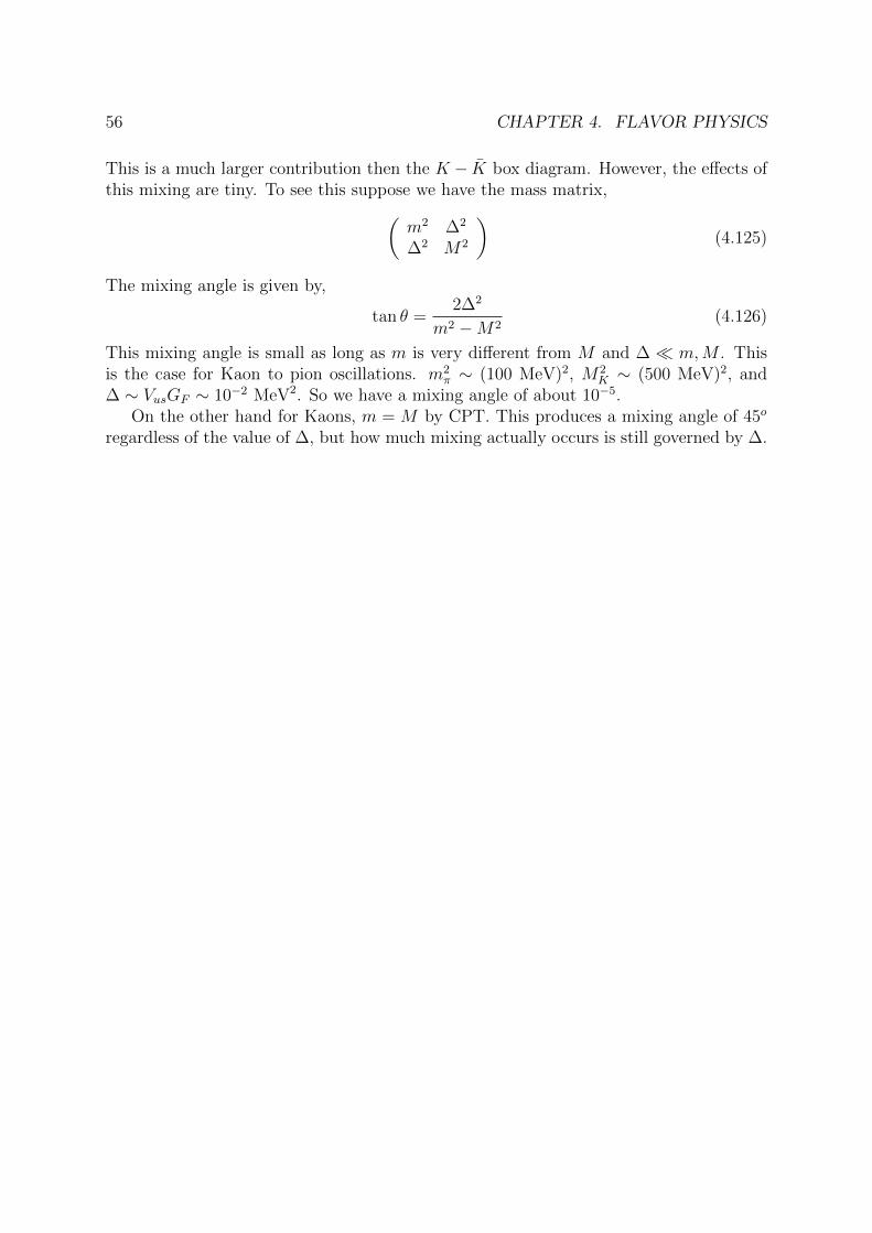
56 CHAPTER 4. FLAVOR PHYSICS
This is a much larger contribution then the K − K box diagram. However, the effects ofthis mixing are tiny. To see this suppose we have the mass matrix,(
m2 ∆2
∆2 M2
)(4.125)
The mixing angle is given by,
tan θ =2∆2
m2 −M2(4.126)
This mixing angle is small as long as m is very different from M and ∆ m,M . Thisis the case for Kaon to pion oscillations. m2
π ∼ (100 MeV)2, M2K ∼ (500 MeV)2, and
∆ ∼ VusGF ∼ 10−2 MeV2. So we have a mixing angle of about 10−5.On the other hand for Kaons, m = M by CPT. This produces a mixing angle of 45o
regardless of the value of ∆, but how much mixing actually occurs is still governed by ∆.
Chapter 5
Neutrino Physics
Unlike all the other topics discussed up to now, the SM doesn’t encode the results of thischapter. Instead people invented the νSM (pronounced as “new Standard Model”).
People have measured,
∆m212 ∼ 10−4eV2 (5.1)
∆m223 ∼ 10−3eV (5.2)
which implies,mν . 10−1eV (5.3)
The massses of the neutrinos are roughly 10−7 smaller then the mass of the electron. Themixing angles are,
θ12 ∼ θ23 ∼ 1, θ13 ∼ 0.1 (5.4)
which is very different then in the quark sector, where there is very little mixing betweendifferent generations.
5.1 Dirac vs Majorana Masses
A mass term couples a right handed field to a left handed field,
mψRψL (5.5)
If ψL 6= ψR then we have a Dirac mass. Alternatively, we can define,
ψc ≡ CψT (5.6)
which changes the chirality of a field. Then we can write,
mψcLCψL (5.7)
However, for this term to exist the field must be neutral under all U(1). Since Q [ψc] =−Q [ψ]. Now suppose that ψ is charged under some non-abelian group instead. Then wehave,
ψ → eiTaαaψ (5.8)
57
58 CHAPTER 5. NEUTRINO PHYSICS
which gives,ψcLCψL → ψcLCe
iT ∗aαaeiTbαbψL (5.9)
which is invariant if −T ∗a = Ta. This is the condition for having a real representation.In the SM the only fields which can be Majorana are the neutrinos. In SUSY the
gauginos as well as the neutral Higgsino can be Majorana.Lets try to understand why neutrino masses are zero in the SM. Firstly we choose
not to include right handed neutrinos which implies that there is no Dirac mass for theright handed neutrinos. Secondly, we assume only a doublet. If we had a triplet scalar,∆(1, 3)1, then we can have a Majorana mass for the neutrinos,
LcL∆LL (5.10)
where L is the lepton doublet. We also choose the SM to be renormalizable. If weincluded dimension 5 operators then we could write,
(HLi)(HLj) (5.11)
We also need to make sure that there is some symmetry to prevent the neutrinos fromgetting mass at loop level and the reason is because U(1)B−L is anomaly free (up to theeffects of gravity).
There are essentially two ways to produce neutrino masses in the SM. We can adda fermion, νR and produce Dirac masses, or a scalar, ∆, which gives Majorana masses.The most naive guess might be Dirac masses,
MN cLNL (5.12)
However, this is highly problematic since there is no good reason for M = 0.If we have a scalar then the neutrino masses are,
mν ∼ λ 〈∆LL〉 (5.13)
The problem is that ∆LL needs to be very small (& GeV) not to interfere with a the ρparameter of EWP and the coupling must also be small.
The modern way to think about adding these heavy degrees of freedom to the SM iswe can write higher dimensional operators to the model. These can be written in termsof the dimension 5 neutrino mass operator above,
λ(HL)2
M⇒ mν =
mv2
M(5.14)
In this modern way of thinking neutrino masses must be there as long as the SM is aneffective theory (unless the UV completian doesn’t give the higher dimensional operator).
The scale of M is apriori unkown. The most naive guess would be M = MPl howeverthen neutrino masses turn out to be too low. There are an infinite number of UVcompletians that contain the dimension 5 operator as an output. The simplest option isthe see-saw mechanism.
5.2. SEE-SAW 59
5.2 See-saw
In this model we add a right handed neutrino, NR(1, 1)0, which implies that we haveadditional terms to the Lagrangian (H ≡ εH∗),
∆L = iNR/∂NR + Y LLHNR +1
2MNN c
RNR (5.15)
After SSB we assume that MN v. One may be concerned that this introduces aheiarachy problem. But we already have the heirarchy problem anyways so adding thisin doesn’t really make the problem any worse.
We make the one generation approximation. We get the mass matrix,
[ νL NR
νL 0 mD
NR m∗D MN
](5.16)
where mD ≡ Y v. To a good approximation the eigenvalues are given by 1,
m1 ≈ −m2D
MN
(5.17)
m2 ≈MN (5.18)
A few remarks:
1. We have a negative mass. However, we can always redefine your fields to eliminatethe phase. The only physical quantity is m†m.
2. The mixing angle is θνN ∼ mD/MN 1. Therefore the mass eigenstate is to a verygood approximation the same as the flavor eigenstate,
|1〉 ≈ |NR〉 |2〉 ≈ |νL〉 (5.19)
3. Matching with the dimension 5 operator we get,
M = MN λ = Y 2 (5.20)
4. If we extend this to 3 flavors we find,
m2D
M→ mT
DM−1mD (5.21)
and,
U →(XNN XNν
XνN Xνν
)(5.22)
XNν is the matrix that generalizes the mixing angle θνN so must be very small,O(mD/M). Since U is the PMNS matrix, in the limit that XNν → 0 limit Xνν isalmost unitary.
1A quick way to diagonalize a two by two matrix is to note that the sum of the eigenvalues shouldbe equal to the trace and the product of the eigenvalues is equal to the determinant.
60 CHAPTER 5. NEUTRINO PHYSICS
5. This model has tree-level flavor changing neutral currents! You can have the pro-cesses:
N → νZ, νH (5.23)
These are typically small since they are suppressed by a mixing angle.
6. What if mD M? In this case you get “sterile neutrinos”. These neutrinos areimportant at low energies but difficult to probe. They can be a form of DM.
This is often called seesaw type I. There are alternatives such as type II where weintroduce a new Higgs as while as seesaw type III where we introduce a new tripletfermion. Each case gives small neutrino masses but has some different phenomenology.
5.3 Neutrino Mixing
Consider some general neutrino masses,
mij νiLν
jR (5.24)
where we νR here is just the chirality symbol we don’t really care here if it is actually aSU(2)L singlet. The charged current interaction is given by,
LW = − g√2
¯L,`U`nγ
µ(νL)nWµ (5.25)
where U is some matrix. ` = e, µ, τ and n = 1, 2, 3. To have neutrino mixing, U must benondiagonal. The matrix breaks the lepton flavor symmetries:
U(1)e × U(1)µ × U(1)τ → U(1)L (5.26)
The mixing itself doesn’t break lepton number (though lepton number violation ofteninevitably appears in the masses, e.g., in the right hand majorana neutrino masses).The mixing matrix has many names, “neutrino mixing matrix”, “PMNS”, “MNS”, or“MNSP”.
The mixing angles of the PMNS matrix are large,
sin θ23 ∼ sin θ12 ∼ O(1) sin θ13 ∼ O(0.1) (5.27)
This is a big difference from the CKM matrix structure. One last difference is the orderof the indices in the mixing matrix. Here we have U`n (charged lepton then neutrinos)(“down” then “up”). However, this is the opposite from the CKM which is defined as,(VCKM)ud. This is just conventional, but important to keep in mind.
In the quark sector we have the up type and down type mass matrices. We chooseto diagonalize mu and md and we choose to keep the charged current nondiagonal. Forthe leptons however, we choose to diagonalize the charged leptons as well as the charged
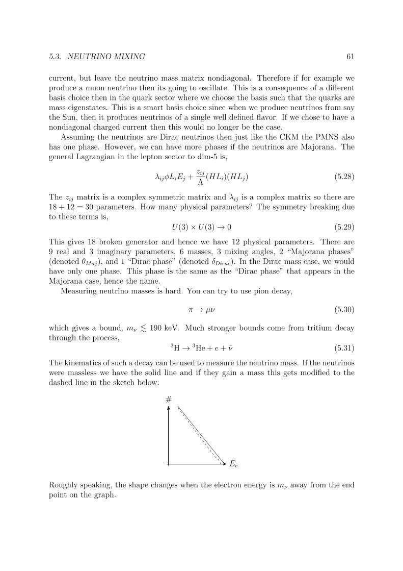
5.3. NEUTRINO MIXING 61
current, but leave the neutrino mass matrix nondiagonal. Therefore if for example weproduce a muon neutrino then its going to oscillate. This is a consequence of a differentbasis choice then in the quark sector where we choose the basis such that the quarks aremass eigenstates. This is a smart basis choice since when we produce neutrinos from saythe Sun, then it produces neutrinos of a single well defined flavor. If we chose to have anondiagonal charged current then this would no longer be the case.
Assuming the neutrinos are Dirac neutrinos then just like the CKM the PMNS alsohas one phase. However, we can have more phases if the neutrinos are Majorana. Thegeneral Lagrangian in the lepton sector to dim-5 is,
λijφLiEj +zijΛ
(HLi)(HLj) (5.28)
The zij matrix is a complex symmetric matrix and λij is a complex matrix so there are18 + 12 = 30 parameters. How many physical parameters? The symmetry breaking dueto these terms is,
U(3)× U(3)→ 0 (5.29)
This gives 18 broken generator and hence we have 12 physical parameters. There are9 real and 3 imaginary parameters, 6 masses, 3 mixing angles, 2 “Majorana phases”(denoted θMaj), and 1 “Dirac phase” (denoted δDirac). In the Dirac mass case, we wouldhave only one phase. This phase is the same as the “Dirac phase” that appears in theMajorana case, hence the name.
Measuring neutrino masses is hard. You can try to use pion decay,
π → µν (5.30)
which gives a bound, mν . 190 keV. Much stronger bounds come from tritium decaythrough the process,
3H→ 3He + e+ ν (5.31)
The kinematics of such a decay can be used to measure the neutrino mass. If the neutrinoswere massless we have the solid line and if they gain a mass this gets modified to thedashed line in the sketch below:
#
Ee
Roughly speaking, the shape changes when the electron energy is mν away from the endpoint on the graph.
62 CHAPTER 5. NEUTRINO PHYSICS
There are two effects. One is that the line shifts down and the other is the changeof shape. Finding the change is shape is in practice much easier to measure. This issomewhat surprising because there are much more events in the rest of the plot. However,since knowing the normalization precisely is very difficult this isn’t feasible. This has beendone to energies, mνe . 2.2eV.
Another way to probe neutrino masses is done by neutrinoless double beta decay(0νββ). β decay is just,
n→ p+ e+ ν (5.32)
Here the neutrino must be present for angular momentum (and lepton number) conser-vation. Another process is ννββ,
2n→ 2p+ 2e+ 2ν (5.33)
In this case angular momentum can be satisfied with or without the neutrinos, they areonly needed for lepton number conservation. 0νββ is,
2n→ 2p+ 2e (5.34)
Beta decay is very common. Two neutrino double beta decay is quite rare. It can onlyoccur if two neutrinos come together and you also have huge phase space surpression.Neutrinoless double beta decay is even more surpressed since they only occur if neutrinosare Majorana fermions, but we do gain some on the phase space.
Remarks:
1. The rate for 0νββ obeys,
Γ ∝ m2ν (5.35)
since it must break lepton number by 2 units. If we have Dirac mass then we don’thave lepton number violation and hence we can’t have this process. 0νββ decayreally measures lepton number violation. In the νSM the only source of leptonnumber is related to the neutrino masses and hence in this model this measures theneutrino mass. The mass is given by,
meββ =
∑miU
2ei (5.36)
Note there is no type here: there is no absolute value signs on Uei.
2. There is theoreoretical uncertainty associated with nuclear matrix elements.
3. It turns out that the best way to study this effect is to use Germanium. In practicewe actually build the detectors out of Germanium and let the Germanium decay.
4. The bounds from this experiment are
mββ . 0.4eV (5.37)
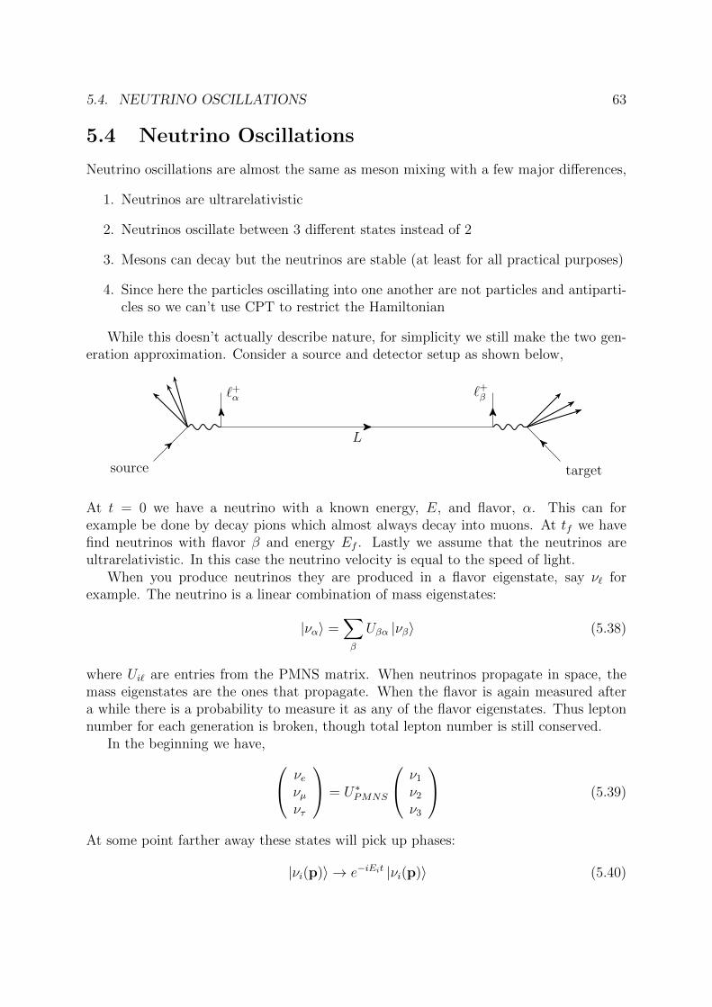
5.4. NEUTRINO OSCILLATIONS 63
5.4 Neutrino Oscillations
Neutrino oscillations are almost the same as meson mixing with a few major differences,
1. Neutrinos are ultrarelativistic
2. Neutrinos oscillate between 3 different states instead of 2
3. Mesons can decay but the neutrinos are stable (at least for all practical purposes)
4. Since here the particles oscillating into one another are not particles and antiparti-cles so we can’t use CPT to restrict the Hamiltonian
While this doesn’t actually describe nature, for simplicity we still make the two gen-eration approximation. Consider a source and detector setup as shown below,
source
L
target
`+α `+
β
At t = 0 we have a neutrino with a known energy, E, and flavor, α. This can forexample be done by decay pions which almost always decay into muons. At tf we havefind neutrinos with flavor β and energy Ef . Lastly we assume that the neutrinos areultrarelativistic. In this case the neutrino velocity is equal to the speed of light.
When you produce neutrinos they are produced in a flavor eigenstate, say ν` forexample. The neutrino is a linear combination of mass eigenstates:
|να〉 =∑β
Uβα |νβ〉 (5.38)
where Ui` are entries from the PMNS matrix. When neutrinos propagate in space, themass eigenstates are the ones that propagate. When the flavor is again measured aftera while there is a probability to measure it as any of the flavor eigenstates. Thus leptonnumber for each generation is broken, though total lepton number is still conserved.
In the beginning we have, νeνµντ
= U∗PMNS
ν1
ν2
ν3
(5.39)
At some point farther away these states will pick up phases:
|νi(p)〉 → e−iEit |νi(p)〉 (5.40)
64 CHAPTER 5. NEUTRINO PHYSICS
where Ei =√
p2 +m2i . Due to this interference between states we have a non-vanishing
probability to find a new type of neutrino. This gives rise to the phenomena of neutrinooscillations. We now answer the question “if you produce a flavor α what is the probabilitythat you will detect a flavor β a given distance away?” We label this probability P (`α →`β).
We derive this result using simple quantum mechanics and treat the neutrinos asplane waves. At some initial time you produce a neutrino is a flavor state;
|να(t0)〉 =∑i
U∗α,i |νi(p)〉 (5.41)
These states are eigenstates of the Hamiltonian and are on shell:
H |νi(p)〉 = Ei |νi(p)〉 (5.42)
Ei =√m2i + p2 ≈ |p|
(1 +
m2i
p2
)(5.43)
We evolve the initial state through the evolution operator:
|να(t)〉 =∑i
U∗αie−iEi(tf−t) |νi(p)〉 (5.44)
The probability is simply
P (να → νβ) = |〈νβ|να(t)〉|2 (5.45)
=
∣∣∣∣∣∑i
Uβ,iU∗α,ie−iEi(tf−t)
∣∣∣∣∣2
(5.46)
The difference of the energies is,
Ej − Ei =√|p|2 +m2
j −√|p|2 +mi (5.47)
≈m2j −m2
i
2 |p|(5.48)
Furthermore,
L = tf − t (5.49)
Inputting in these results gives the master formula:
P (να → νβ) =∑ij
U∗β,jUα,jUβ,iU∗α,ie
i∆m2jiL/2|p| (5.50)
The master formula gives the “probability of appearance” for α 6= β and the “probabilityof dissappearance” for α = β. One can show that the master formula can be written
5.4. NEUTRINO OSCILLATIONS 65
in a slightly more famililar form using the Unitarity of the matrix: [Q 27: Derive thisformula.]
P (να → νβ) = δαβ − 4∑i<j
Re[U∗α,iUβ,iUα,jU
∗β,j
]sin2
∆m2ijL
4E
− 2∑i<j
Im[U∗α,iUβ,iUα,jU
∗β,j
]sin
∆m2ijL
2E(5.51)
To compute the corresponding formula for neutrinos we just need to take the complexconjugate of the product of matrix. This gives,
P (να → νβ) = δαβ − 4∑i<j
Re[U∗α,iUβ,iUα,jU
∗β,j
]sin2
∆m2ijL
4E
+ 2∑i<j
Im[U∗α,iUβ,iUα,jU
∗β,j
]sin
∆m2ijL
2E(5.52)
Thus to the extent that the imaginary term does not vanish we will have a difference inthe oscillation probability for neutrinos and antineutrinos. In order to avoid this termthe phases in the imaginary parts need to add to zero. It is a simple exercise to showthat in the case that ∆m = 0 for one set of the neutrinos this term vanishes.
For only two generations there is one angle in the mixing matrix and its given by,
U =
(cos θ − sin θsin θ cos θ
)(5.53)
Plugging in to the result above for disappearance2
P (να → νβ) = sin2 2θ sin2 ∆m2L
4E= sin2 2θ sin2
(1.27∆m2(eV)L(km)
E(GeV)
)(5.54)
This formula can be easily understood. You’ll have more oscillation if the mass differ-ences are greater or you have a longer beamline. Furthermore, we have a 1/E due to atime dialation factor. The greater the energy, the shorter the beamline appears to theneutrinos. The oscillation length is,
λ ≡ 2πE
∆m2(5.55)
Lets consider some limits:L λ P (να → νβ)→ 0L λ P (να → νβ)→ 1
2sin2 2θ
L ∼ λ P (να → νβ)→ sin2 2θ sin2 ∆m2L4E
(5.56)
For GeV neutrinos with a beamline of 1 km we see 1 oscillation. To get more oscilla-tions we want to minimize the energy and large beamlines. Then we can probe smaller∆m2.
2It helps to note that for i > j we can only have i = 1, j = 2.
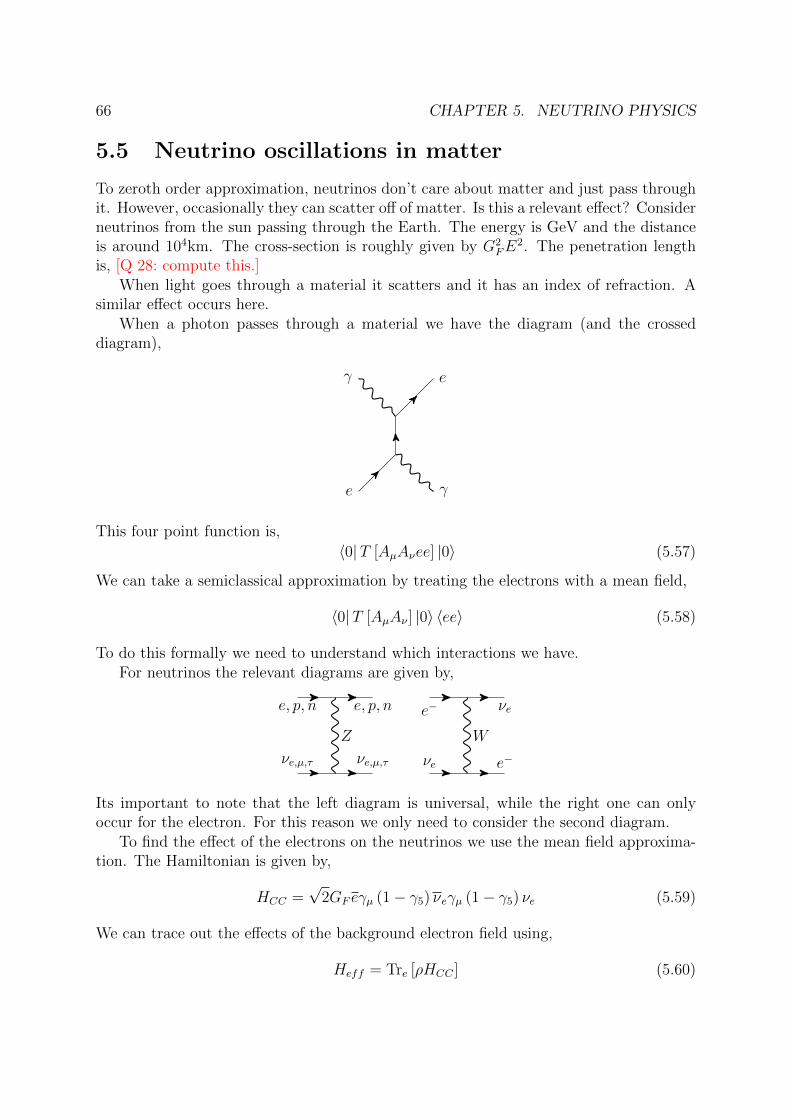
66 CHAPTER 5. NEUTRINO PHYSICS
5.5 Neutrino oscillations in matter
To zeroth order approximation, neutrinos don’t care about matter and just pass throughit. However, occasionally they can scatter off of matter. Is this a relevant effect? Considerneutrinos from the sun passing through the Earth. The energy is GeV and the distanceis around 104km. The cross-section is roughly given by G2
FE2. The penetration length
is, [Q 28: compute this.]When light goes through a material it scatters and it has an index of refraction. A
similar effect occurs here.When a photon passes through a material we have the diagram (and the crossed
diagram),
e
γ e
γ
This four point function is,
〈0|T [AµAνee] |0〉 (5.57)
We can take a semiclassical approximation by treating the electrons with a mean field,
〈0|T [AµAν ] |0〉 〈ee〉 (5.58)
To do this formally we need to understand which interactions we have.For neutrinos the relevant diagrams are given by,
νe,µ,τ νe,µ,τ
Z
e, p, n e, p, n
νe e−
W
e− νe
Its important to note that the left diagram is universal, while the right one can onlyoccur for the electron. For this reason we only need to consider the second diagram.
To find the effect of the electrons on the neutrinos we use the mean field approxima-tion. The Hamiltonian is given by,
HCC =√
2GF eγµ (1− γ5) νeγµ (1− γ5) νe (5.59)
We can trace out the effects of the background electron field using,
Heff = Tre [ρHCC ] (5.60)
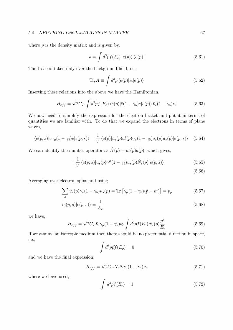
5.5. NEUTRINO OSCILLATIONS IN MATTER 67
where ρ is the density matrix and is given by,
ρ =
∫d3pf(Ee) |e(p)〉 〈e(p)| (5.61)
The trace is taken only over the background field, i.e.
TreA ≡∫d3p 〈e(p)|A|e(p)〉 (5.62)
Inserting these relations into the above we have the Hamiltonian,
Heff =√
2GF
∫d3pf(Ee) 〈e(p)|e(1− γ5)e|e(p)〉 νe(1− γ5)νe (5.63)
We now need to simplify the expression for the electron braket and put it in terms ofquantities we are familiar with. To do that we expand the electrons in terms of planewaves,
〈e(p, s)|eγµ(1− γ5)e|e(p, s)〉 =1
V〈e(p)|us(p)a†s(p)γµ(1− γ5)as(p)us(p)|e(p, s)〉 (5.64)
We can identify the number operator as N(p) = a†(p)a(p), which gives,
=1
V〈e(p, s)|us(p)γµ(1− γ5)us(p)Ne(p)|e(p, s)〉 (5.65)
(5.66)
Averaging over electron spins and using∑s
us(p)γµ(1− γ5)us(p) = Tr[γµ(1− γ5)(/p−m)
]= pµ (5.67)
〈e(p, s)|e(p, s)〉 =1
Ee(5.68)
we have,
Heff =√
2GF νeγµ(1− γ5)νe
∫d3pf(Ee)Ne(p)
pµ
Ee(5.69)
If we assume an isotropic medium then there should be no preferential direction in space,i.e., ∫
d3p~pf(Ep) = 0 (5.70)
and we have the final expression,
Heff =√
2GFNeνeγ0(1− γ5)νe (5.71)
where we have used, ∫d3pf(Ee) = 1 (5.72)
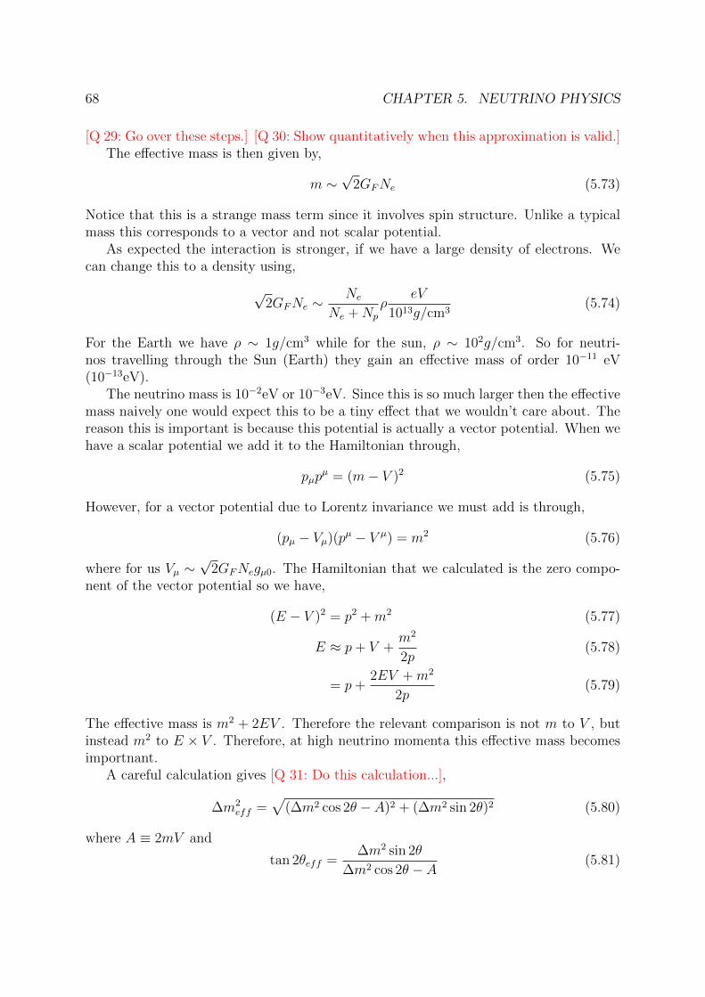
68 CHAPTER 5. NEUTRINO PHYSICS
[Q 29: Go over these steps.] [Q 30: Show quantitatively when this approximation is valid.]The effective mass is then given by,
m ∼√
2GFNe (5.73)
Notice that this is a strange mass term since it involves spin structure. Unlike a typicalmass this corresponds to a vector and not scalar potential.
As expected the interaction is stronger, if we have a large density of electrons. Wecan change this to a density using,
√2GFNe ∼
Ne
Ne +Np
ρeV
1013g/cm3(5.74)
For the Earth we have ρ ∼ 1g/cm3 while for the sun, ρ ∼ 102g/cm3. So for neutri-nos travelling through the Sun (Earth) they gain an effective mass of order 10−11 eV(10−13eV).
The neutrino mass is 10−2eV or 10−3eV. Since this is so much larger then the effectivemass naively one would expect this to be a tiny effect that we wouldn’t care about. Thereason this is important is because this potential is actually a vector potential. When wehave a scalar potential we add it to the Hamiltonian through,
pµpµ = (m− V )2 (5.75)
However, for a vector potential due to Lorentz invariance we must add is through,
(pµ − Vµ)(pµ − V µ) = m2 (5.76)
where for us Vµ ∼√
2GFNegµ0. The Hamiltonian that we calculated is the zero compo-nent of the vector potential so we have,
(E − V )2 = p2 +m2 (5.77)
E ≈ p+ V +m2
2p(5.78)
= p+2EV +m2
2p(5.79)
The effective mass is m2 + 2EV . Therefore the relevant comparison is not m to V , butinstead m2 to E × V . Therefore, at high neutrino momenta this effective mass becomesimportnant.
A careful calculation gives [Q 31: Do this calculation...],
∆m2eff =
√(∆m2 cos 2θ − A)2 + (∆m2 sin 2θ)2 (5.80)
where A ≡ 2mV and
tan 2θeff =∆m2 sin 2θ
∆m2 cos 2θ − A(5.81)
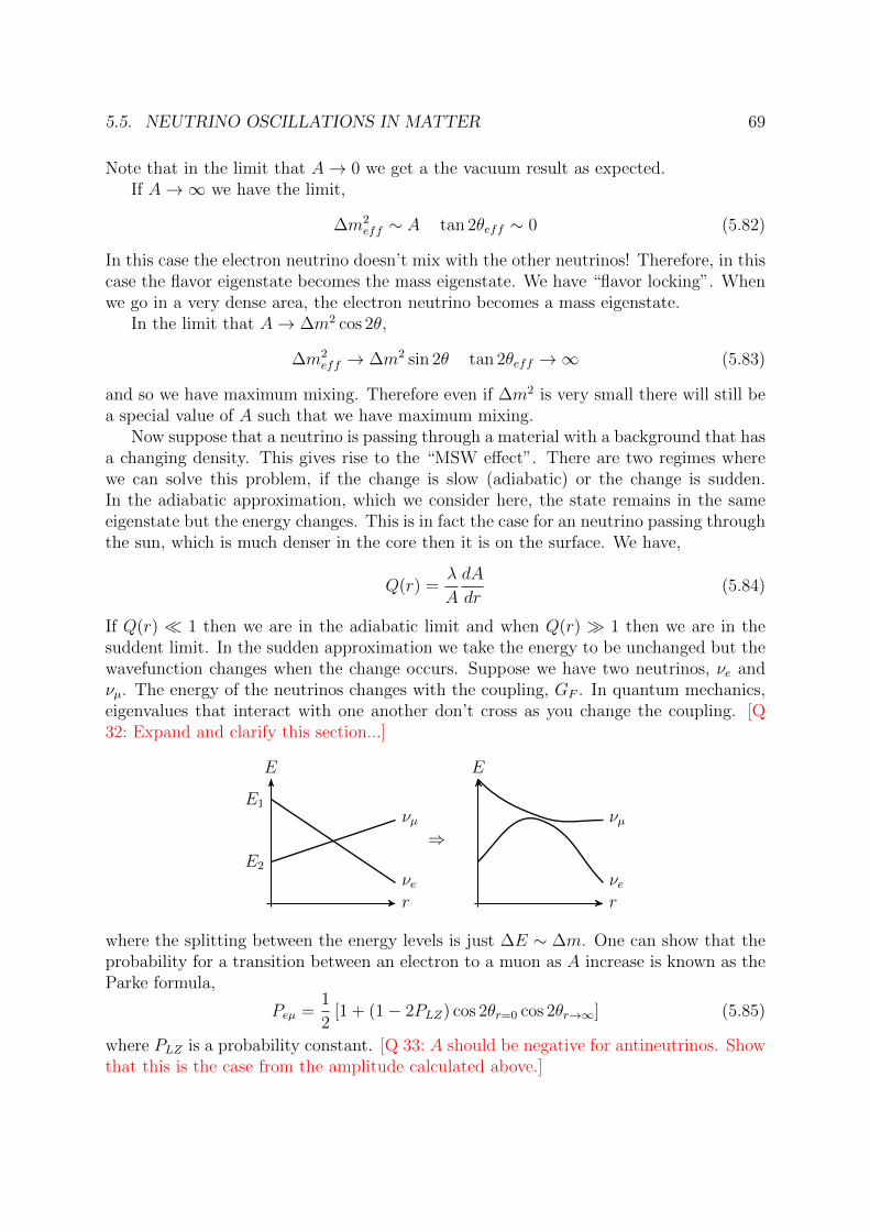
5.5. NEUTRINO OSCILLATIONS IN MATTER 69
Note that in the limit that A→ 0 we get a the vacuum result as expected.If A→∞ we have the limit,
∆m2eff ∼ A tan 2θeff ∼ 0 (5.82)
In this case the electron neutrino doesn’t mix with the other neutrinos! Therefore, in thiscase the flavor eigenstate becomes the mass eigenstate. We have “flavor locking”. Whenwe go in a very dense area, the electron neutrino becomes a mass eigenstate.
In the limit that A→ ∆m2 cos 2θ,
∆m2eff → ∆m2 sin 2θ tan 2θeff →∞ (5.83)
and so we have maximum mixing. Therefore even if ∆m2 is very small there will still bea special value of A such that we have maximum mixing.
Now suppose that a neutrino is passing through a material with a background that hasa changing density. This gives rise to the “MSW effect”. There are two regimes wherewe can solve this problem, if the change is slow (adiabatic) or the change is sudden.In the adiabatic approximation, which we consider here, the state remains in the sameeigenstate but the energy changes. This is in fact the case for an neutrino passing throughthe sun, which is much denser in the core then it is on the surface. We have,
Q(r) =λ
A
dA
dr(5.84)
If Q(r) 1 then we are in the adiabatic limit and when Q(r) 1 then we are in thesuddent limit. In the sudden approximation we take the energy to be unchanged but thewavefunction changes when the change occurs. Suppose we have two neutrinos, νe andνµ. The energy of the neutrinos changes with the coupling, GF . In quantum mechanics,eigenvalues that interact with one another don’t cross as you change the coupling. [Q32: Expand and clarify this section...]
E
r
E2
νµE1
νe
⇒
E
r
νe
νµ
where the splitting between the energy levels is just ∆E ∼ ∆m. One can show that theprobability for a transition between an electron to a muon as A increase is known as theParke formula,
Peµ =1
2[1 + (1− 2PLZ) cos 2θr=0 cos 2θr→∞] (5.85)
where PLZ is a probability constant. [Q 33: A should be negative for antineutrinos. Showthat this is the case from the amplitude calculated above.]
70 CHAPTER 5. NEUTRINO PHYSICS
5.6 Neutrino oscillation experiments
The big issue with neutrino oscillation experiments is that the cross section of neutrinointeractions with the detectors is very small. To solve this problem we can do two things,
1. Increase the size of the target
2. Bring the source close to the target so all the neutrinos hit the target
On the other hand the oscillation frequency scales inversely with the length of theexperiment. Therefore, we don’t want to bring the target too close that we don’t seeoscillation but not too far so we don’t lose too many neutrinos.
Next consider the neutrino energy. The cross section of Fermi interaction increaseswith the energy. Furthermore, the higher energy beam that you have, the easier it is tofocus the beam. On the other hand, we also would like to have low energy neutrinos sincelower energy neutrinos oscillate more. This is just because of special relativity. For veryfast moving neutrinos, the length of the beam line is contracted by a γ factor. Therefore,similarly for the length of the beamline, we again have a competition.
For an initial beam we want to know the energy, the flux, as well as the flavor. Wethen detect each of these quantity for the final beam.
In general there are two types of neutrino oscillation experiments. The one typeis called appearance exeriments. In this set of experiments you start with some flavorNα(t = 0) = 0 and find that at some time tf after Nα(tf ) 6= 0. For this experiment theflux cancels out when calculating physical quantities. Therefore, the important propertiesfor these types of experiments is the energy of length of the beamline. For disappearanceexperiment we start with Nα(t = 0) and check how many neutrinos of flavor α we haveat some time tf . Here the flux is important.
An interesting test of neutrinos comes from looking at the Sun. The photons in thesun have a very difficult time getting out of the Sun due to all the interactions withmatter. The time it takes a photon to leave the center of the Sun and arrive on Earth isroughly a billion years. On the other hand, because neutrinos don’t interact the time ittakes neutrinos to go from the Sun to the Earth is about 8 minutes.
At the sun we know the flavor of the neutrinos very well since its dominated byelectron neutrinos. Note that fusion tends to come with neutrinos while fission tends tocome with antineutrinos. The energy is roughly given by the scale of nuclear physics,MeV. We certainly can’t produce muons which have a mass of about 100MeV. The basicprocess is given by,
4p→ 4He + 2e+ + 2νe + 2γ (5.86)
The 98.5% of the neutrinos have an energy, Eν < 0.. The problem is that experimentallyis very hard to go to such small neutrino energies. The first generation of experimentswasn’t able to probe these low energy neutrinos.
One detection mechanism is known as the charged current interaction,
νe + n→ p+ e− (5.87)
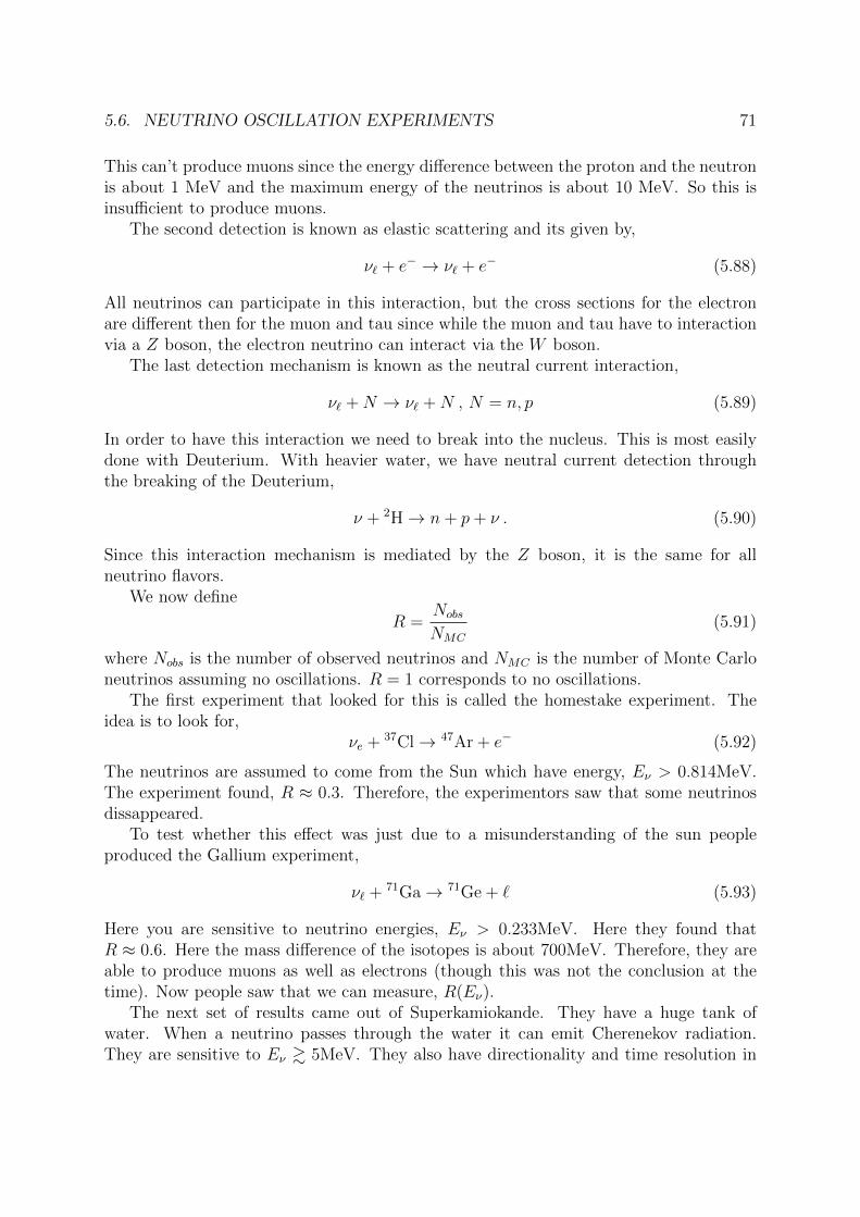
5.6. NEUTRINO OSCILLATION EXPERIMENTS 71
This can’t produce muons since the energy difference between the proton and the neutronis about 1 MeV and the maximum energy of the neutrinos is about 10 MeV. So this isinsufficient to produce muons.
The second detection is known as elastic scattering and its given by,
ν` + e− → ν` + e− (5.88)
All neutrinos can participate in this interaction, but the cross sections for the electronare different then for the muon and tau since while the muon and tau have to interactionvia a Z boson, the electron neutrino can interact via the W boson.
The last detection mechanism is known as the neutral current interaction,
ν` +N → ν` +N , N = n, p (5.89)
In order to have this interaction we need to break into the nucleus. This is most easilydone with Deuterium. With heavier water, we have neutral current detection throughthe breaking of the Deuterium,
ν + 2H→ n+ p+ ν . (5.90)
Since this interaction mechanism is mediated by the Z boson, it is the same for allneutrino flavors.
We now define
R =Nobs
NMC
(5.91)
where Nobs is the number of observed neutrinos and NMC is the number of Monte Carloneutrinos assuming no oscillations. R = 1 corresponds to no oscillations.
The first experiment that looked for this is called the homestake experiment. Theidea is to look for,
νe + 37Cl→ 47Ar + e− (5.92)
The neutrinos are assumed to come from the Sun which have energy, Eν > 0.814MeV.The experiment found, R ≈ 0.3. Therefore, the experimentors saw that some neutrinosdissappeared.
To test whether this effect was just due to a misunderstanding of the sun peopleproduced the Gallium experiment,
ν` + 71Ga→ 71Ge + ` (5.93)
Here you are sensitive to neutrino energies, Eν > 0.233MeV. Here they found thatR ≈ 0.6. Here the mass difference of the isotopes is about 700MeV. Therefore, they areable to produce muons as well as electrons (though this was not the conclusion at thetime). Now people saw that we can measure, R(Eν).
The next set of results came out of Superkamiokande. They have a huge tank ofwater. When a neutrino passes through the water it can emit Cherenekov radiation.They are sensitive to Eν & 5MeV. They also have directionality and time resolution in
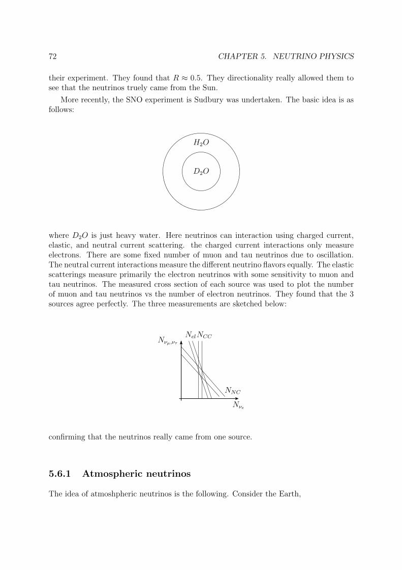
72 CHAPTER 5. NEUTRINO PHYSICS
their experiment. They found that R ≈ 0.5. They directionality really allowed them tosee that the neutrinos truely came from the Sun.
More recently, the SNO experiment is Sudbury was undertaken. The basic idea is asfollows:
D2O
H2O
where D2O is just heavy water. Here neutrinos can interaction using charged current,elastic, and neutral current scattering. the charged current interactions only measureelectrons. There are some fixed number of muon and tau neutrinos due to oscillation.The neutral current interactions measure the different neutrino flavors equally. The elasticscatterings measure primarily the electron neutrinos with some sensitivity to muon andtau neutrinos. The measured cross section of each source was used to plot the numberof muon and tau neutrinos vs the number of electron neutrinos. They found that the 3sources agree perfectly. The three measurements are sketched below:
Nνµ,ντ
Nνe
NCCNel
NNC
confirming that the neutrinos really came from one source.
5.6.1 Atmospheric neutrinos
The idea of atmoshpheric neutrinos is the following. Consider the Earth,
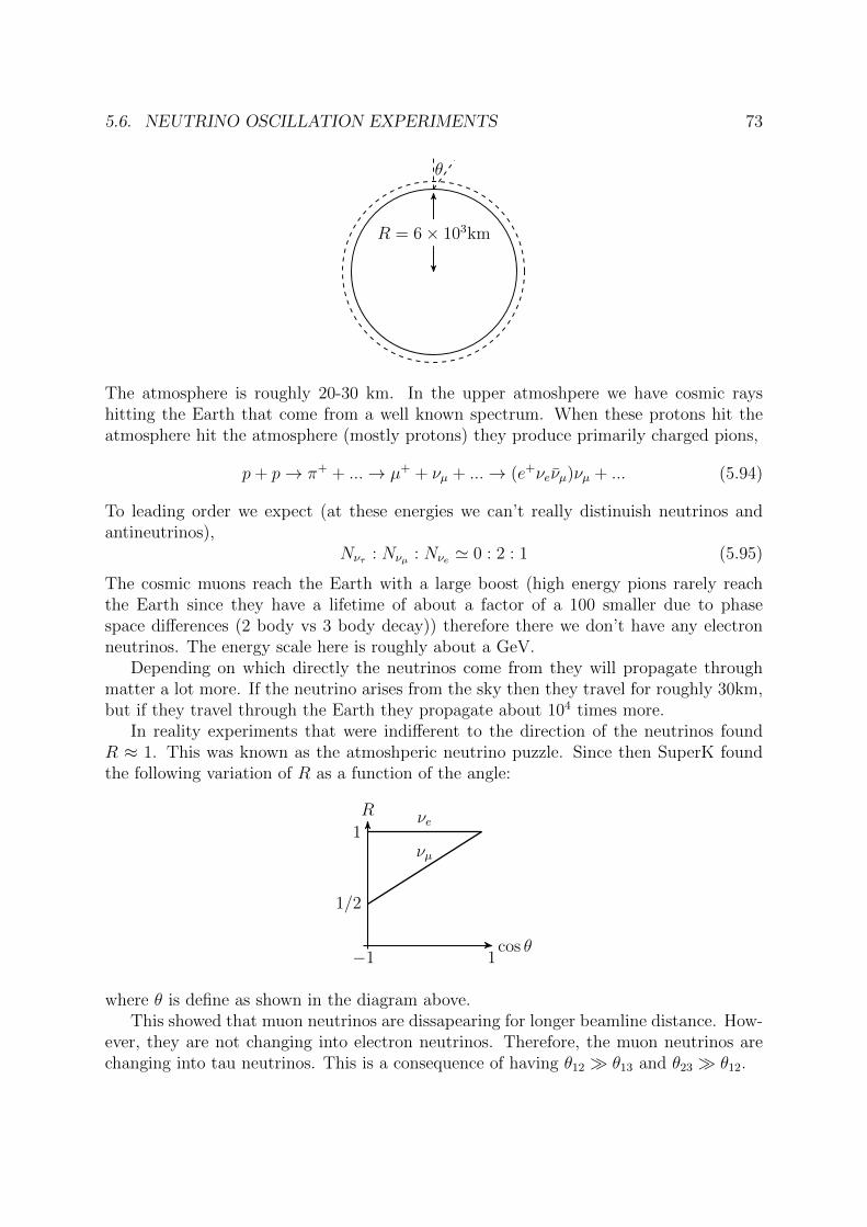
5.6. NEUTRINO OSCILLATION EXPERIMENTS 73
R = 6× 10³km
θ
The atmosphere is roughly 20-30 km. In the upper atmoshpere we have cosmic rayshitting the Earth that come from a well known spectrum. When these protons hit theatmosphere hit the atmosphere (mostly protons) they produce primarily charged pions,
p+ p→ π+ + ...→ µ+ + νµ + ...→ (e+νeνµ)νµ + ... (5.94)
To leading order we expect (at these energies we can’t really distinuish neutrinos andantineutrinos),
Nντ : Nνµ : Nνe ' 0 : 2 : 1 (5.95)
The cosmic muons reach the Earth with a large boost (high energy pions rarely reachthe Earth since they have a lifetime of about a factor of a 100 smaller due to phasespace differences (2 body vs 3 body decay)) therefore there we don’t have any electronneutrinos. The energy scale here is roughly about a GeV.
Depending on which directly the neutrinos come from they will propagate throughmatter a lot more. If the neutrino arises from the sky then they travel for roughly 30km,but if they travel through the Earth they propagate about 104 times more.
In reality experiments that were indifferent to the direction of the neutrinos foundR ≈ 1. This was known as the atmoshperic neutrino puzzle. Since then SuperK foundthe following variation of R as a function of the angle:
R
−1 1cos θ
1νe
1/2
νµ
where θ is define as shown in the diagram above.This showed that muon neutrinos are dissapearing for longer beamline distance. How-
ever, they are not changing into electron neutrinos. Therefore, the muon neutrinos arechanging into tau neutrinos. This is a consequence of having θ12 θ13 and θ23 θ12.
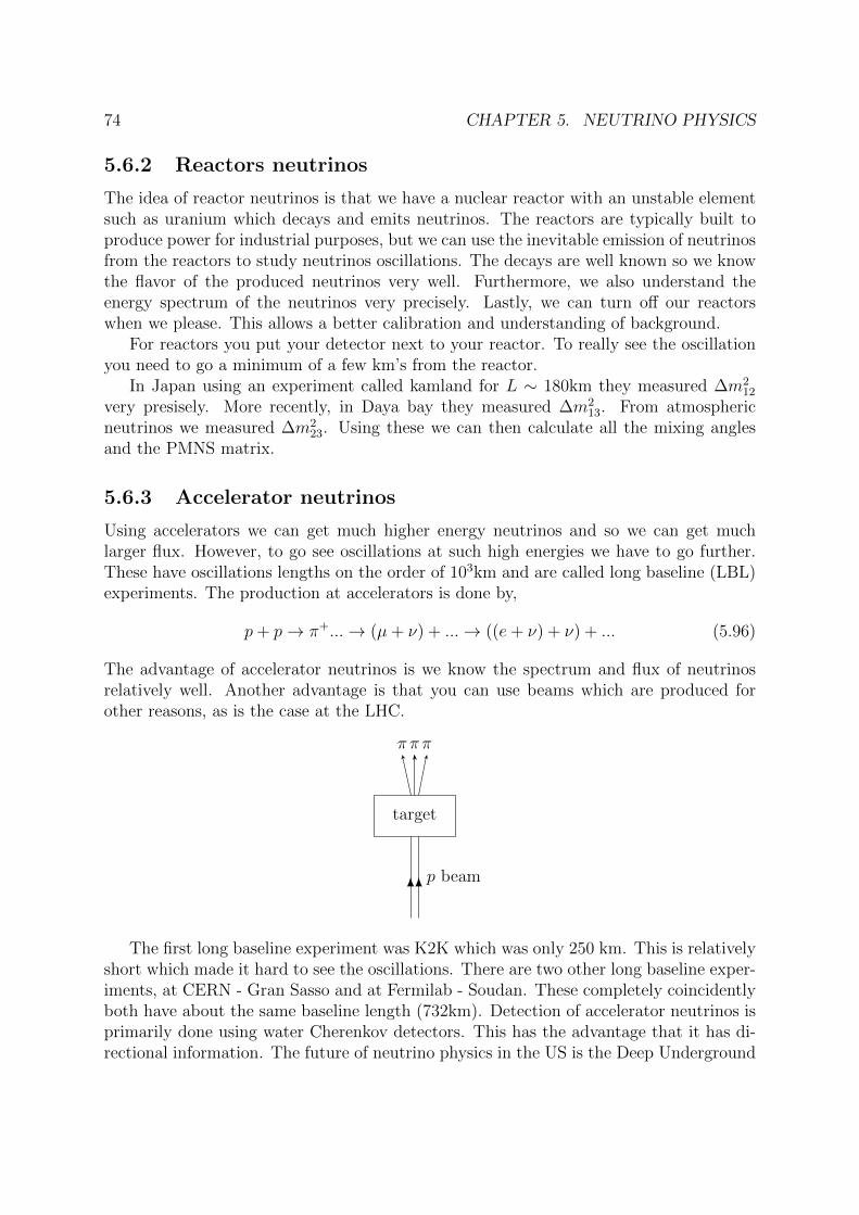
74 CHAPTER 5. NEUTRINO PHYSICS
5.6.2 Reactors neutrinos
The idea of reactor neutrinos is that we have a nuclear reactor with an unstable elementsuch as uranium which decays and emits neutrinos. The reactors are typically built toproduce power for industrial purposes, but we can use the inevitable emission of neutrinosfrom the reactors to study neutrinos oscillations. The decays are well known so we knowthe flavor of the produced neutrinos very well. Furthermore, we also understand theenergy spectrum of the neutrinos very precisely. Lastly, we can turn off our reactorswhen we please. This allows a better calibration and understanding of background.
For reactors you put your detector next to your reactor. To really see the oscillationyou need to go a minimum of a few km’s from the reactor.
In Japan using an experiment called kamland for L ∼ 180km they measured ∆m212
very presisely. More recently, in Daya bay they measured ∆m213. From atmospheric
neutrinos we measured ∆m223. Using these we can then calculate all the mixing angles
and the PMNS matrix.
5.6.3 Accelerator neutrinos
Using accelerators we can get much higher energy neutrinos and so we can get muchlarger flux. However, to go see oscillations at such high energies we have to go further.These have oscillations lengths on the order of 103km and are called long baseline (LBL)experiments. The production at accelerators is done by,
p+ p→ π+...→ (µ+ ν) + ...→ ((e+ ν) + ν) + ... (5.96)
The advantage of accelerator neutrinos is we know the spectrum and flux of neutrinosrelatively well. Another advantage is that you can use beams which are produced forother reasons, as is the case at the LHC.
p beam
πππ
target
The first long baseline experiment was K2K which was only 250 km. This is relativelyshort which made it hard to see the oscillations. There are two other long baseline exper-iments, at CERN - Gran Sasso and at Fermilab - Soudan. These completely coincidentlyboth have about the same baseline length (732km). Detection of accelerator neutrinos isprimarily done using water Cherenkov detectors. This has the advantage that it has di-rectional information. The future of neutrino physics in the US is the Deep Underground
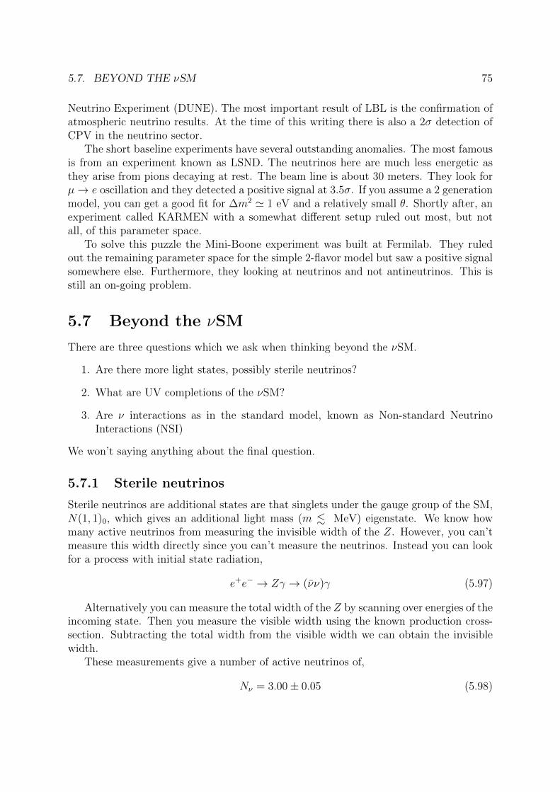
5.7. BEYOND THE νSM 75
Neutrino Experiment (DUNE). The most important result of LBL is the confirmation ofatmospheric neutrino results. At the time of this writing there is also a 2σ detection ofCPV in the neutrino sector.
The short baseline experiments have several outstanding anomalies. The most famousis from an experiment known as LSND. The neutrinos here are much less energetic asthey arise from pions decaying at rest. The beam line is about 30 meters. They look forµ→ e oscillation and they detected a positive signal at 3.5σ. If you assume a 2 generationmodel, you can get a good fit for ∆m2 ' 1 eV and a relatively small θ. Shortly after, anexperiment called KARMEN with a somewhat different setup ruled out most, but notall, of this parameter space.
To solve this puzzle the Mini-Boone experiment was built at Fermilab. They ruledout the remaining parameter space for the simple 2-flavor model but saw a positive signalsomewhere else. Furthermore, they looking at neutrinos and not antineutrinos. This isstill an on-going problem.
5.7 Beyond the νSM
There are three questions which we ask when thinking beyond the νSM.
1. Are there more light states, possibly sterile neutrinos?
2. What are UV completions of the νSM?
3. Are ν interactions as in the standard model, known as Non-standard NeutrinoInteractions (NSI)
We won’t saying anything about the final question.
5.7.1 Sterile neutrinos
Sterile neutrinos are additional states are that singlets under the gauge group of the SM,N(1, 1)0, which gives an additional light mass (m . MeV) eigenstate. We know howmany active neutrinos from measuring the invisible width of the Z. However, you can’tmeasure this width directly since you can’t measure the neutrinos. Instead you can lookfor a process with initial state radiation,
e+e− → Zγ → (νν)γ (5.97)
Alternatively you can measure the total width of the Z by scanning over energies of theincoming state. Then you measure the visible width using the known production cross-section. Subtracting the total width from the visible width we can obtain the invisiblewidth.
These measurements give a number of active neutrinos of,
Nν = 3.00± 0.05 (5.98)
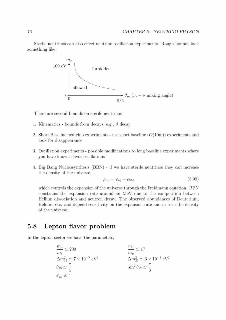
76 CHAPTER 5. NEUTRINO PHYSICS
Sterile neutrinos can also effect neutrino oscillation experiments. Rough bounds looksomething like:
ms
θsa (νs − ν mixing angle)0
0π/4
100 eV
allowed
forbidden
There are several bounds on sterile neutrinos
1. Kinematics - bounds from decays, e.g., β decay
2. Short Baseline neutrino experiments - use short baseline (O(10m)) experiments andlook for disappearance
3. Oscillation experiments - possible modifications to long baseline experiments whereyou have known flavor oscillations
4. Big Bang Nucleosynthesis (BBN) - if we have sterile neutrinos they can increasethe density of the universe,
ρtot = ρνs + ρSM (5.99)
which controls the expansion of the universe through the Freidmann equation. BBNconstrains the expansion rate around an MeV due to the competition betweenHelium dissociation and neutron decay. The observed abundances of Deuterium,Helium, etc. and depend sensitivity on the expansion rate and in turn the densityof the universe.
5.8 Lepton flavor problem
In the lepton sector we have the parameters,
mµ
me
' 200mτ
mµ
' 17
∆m212 ' 7× 10⁻⁵ eV2 ∆m2
23 ' 3× 10⁻³ eV2
θ23 'π
4sin2 θ12 '
π
3θ13 1
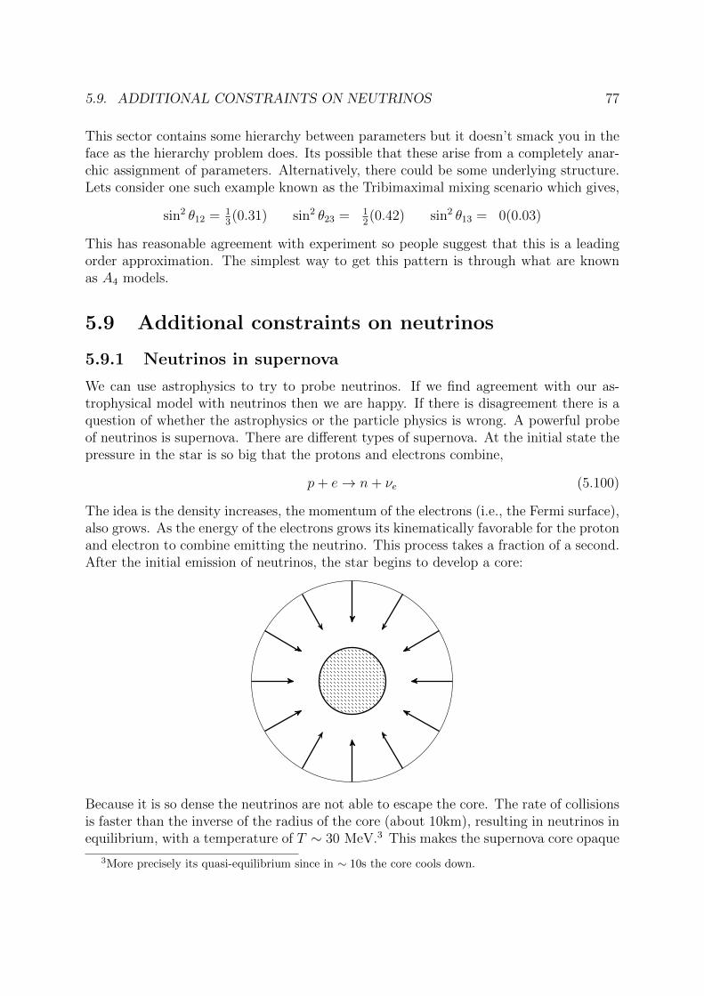
5.9. ADDITIONAL CONSTRAINTS ON NEUTRINOS 77
This sector contains some hierarchy between parameters but it doesn’t smack you in theface as the hierarchy problem does. Its possible that these arise from a completely anar-chic assignment of parameters. Alternatively, there could be some underlying structure.Lets consider one such example known as the Tribimaximal mixing scenario which gives,
sin2 θ12 = 13(0.31) sin2 θ23 = 1
2(0.42) sin2 θ13 = 0(0.03)
This has reasonable agreement with experiment so people suggest that this is a leadingorder approximation. The simplest way to get this pattern is through what are knownas A4 models.
5.9 Additional constraints on neutrinos
5.9.1 Neutrinos in supernova
We can use astrophysics to try to probe neutrinos. If we find agreement with our as-trophysical model with neutrinos then we are happy. If there is disagreement there is aquestion of whether the astrophysics or the particle physics is wrong. A powerful probeof neutrinos is supernova. There are different types of supernova. At the initial state thepressure in the star is so big that the protons and electrons combine,
p+ e→ n+ νe (5.100)
The idea is the density increases, the momentum of the electrons (i.e., the Fermi surface),also grows. As the energy of the electrons grows its kinematically favorable for the protonand electron to combine emitting the neutrino. This process takes a fraction of a second.After the initial emission of neutrinos, the star begins to develop a core:
Because it is so dense the neutrinos are not able to escape the core. The rate of collisionsis faster than the inverse of the radius of the core (about 10km), resulting in neutrinos inequilibrium, with a temperature of T ∼ 30 MeV.3 This makes the supernova core opaque
3More precisely its quasi-equilibrium since in ∼ 10s the core cools down.
78 CHAPTER 5. NEUTRINO PHYSICS
to neutrinos. This is analogous to what happens in the sun for photons. The photons inthe sun are stuck since the rate of collisions in so large.
The supersnova core (also known as the “neutrino sphere”) is different from the elec-tron and muon (or tau) neutrinos. The reason is that cross-section to collide with electronsis different for the different type of neutrinos.
The most famous supernova is probably supernova 1987A. This was a supernova in theMangellanic cloud. It was not in our galaxy but it was close enough. Superkamiokandewas able to observe about 20 events. They saw potentially a faint signal from the initialsupernova collapse but saw a very clear signal from the supernova core. There are a fewbounds we can derive from this event,
1. Stability: since the distance to the supernova was ∼ 170 000 light years we knowthe neutrino lifetime is roughly longer then 105 years.
2. Mass difference: to our experimental sensitivity we found the neutrino beams comeall in the single bunch. If there mass difference was large, then we would get 3separate bunches. This allowed us to put a constraint of O(10 eV) on the massdifference
3. Neutrino magnetic moment: If the neutrino is a Dirac neutrino it will have a mag-netic moment which will interact with the magnetic field of the universe.
4. Lorentz invariance violation: Lorentz invariance tells us that the velocity of theneutrino will be independent of the direction of the proton that created it. We cancheck this using these supernova neutrinos. This is actually the best bounds wehave on Lorentz invariance violation.
the nuetr
5.9.2 Neutrino dark matter
Neutrinos are a form of dark matter so in principle they could account for the extramatter in the universe. If the neutrino were heavier, with a mass around 20 eV, then itcould account for the extra energy density observed today in dark matter. However thisis ruled out for additional reason, because we observe small scale structure which wouldbe inconsistent with hot dark matter. We can use this to put an additional constraint onneutrino masses
5.10 Bounds on new physics
All this section we discussed the SM unique dimension 5 operator,
LHLH
M(5.101)
5.10. BOUNDS ON NEW PHYSICS 79
There are many dimension 6 operators. Flavor conserving operators are bound by EWP,flavor violating operators are bound by meson measurements, and baryon/lepton numberviolation is bound through proton decay.
We spoke in depth about all of the operators except the ones correponding to protondecay bounds. One such operator is,
QQQL
M2(5.102)
This could give proton decay through,
p→ e+γ, p→ e+π0 (5.103)
In principle since these operators are dimension 6 they should give a much weaker boundon the scale M . However experimentally, proton decay is very easy to probe. For thisreason, the strongest bound on M (from proton decay) gives, M & 1016GeV.
To have proton decay we actually need both baryon and lepton number violation.The reason is that the proton needs a (assymptotically free) fermion to decay to and inthe SM the only fermions lighter then the proton are the leptons. This is actually a bittoo strong a statement since we could have for example decays to the gravitino whichwould be invisible.
The proton decay operators are ∆B = ∆L = 1. There are also experiments whichprobe ∆B = 2,∆L = 0. One such experiment looks for n − n oscillation. Anotherexample looks for,
16O → 16C + π+π− (5.104)
The bound on these are much weaker then on proton decay.
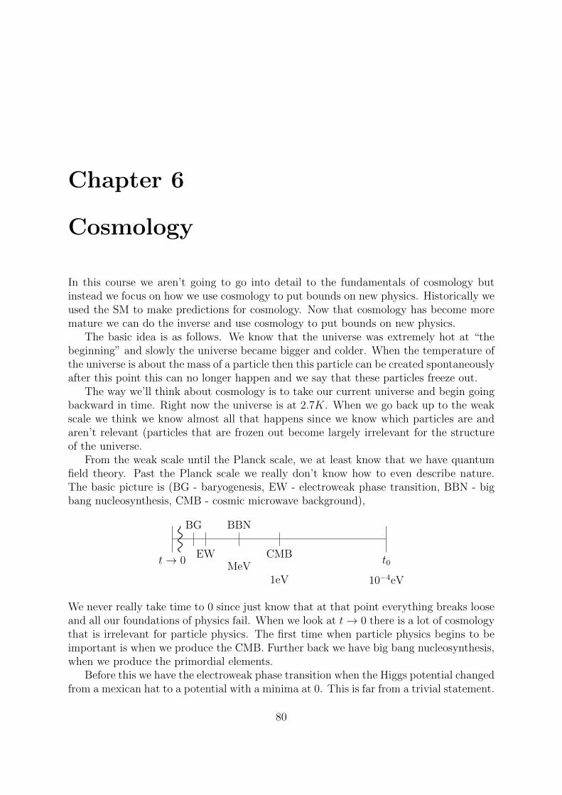
Chapter 6
Cosmology
In this course we aren’t going to go into detail to the fundamentals of cosmology butinstead we focus on how we use cosmology to put bounds on new physics. Historically weused the SM to make predictions for cosmology. Now that cosmology has become moremature we can do the inverse and use cosmology to put bounds on new physics.
The basic idea is as follows. We know that the universe was extremely hot at “thebeginning” and slowly the universe became bigger and colder. When the temperature ofthe universe is about the mass of a particle then this particle can be created spontaneouslyafter this point this can no longer happen and we say that these particles freeze out.
The way we’ll think about cosmology is to take our current universe and begin goingbackward in time. Right now the universe is at 2.7K. When we go back up to the weakscale we think we know almost all that happens since we know which particles are andaren’t relevant (particles that are frozen out become largely irrelevant for the structureof the universe.
From the weak scale until the Planck scale, we at least know that we have quantumfield theory. Past the Planck scale we really don’t know how to even describe nature.The basic picture is (BG - baryogenesis, EW - electroweak phase transition, BBN - bigbang nucleosynthesis, CMB - cosmic microwave background),
t→ 0 t0CMB
BBN
EW
BG
10−4eV1eVMeV
We never really take time to 0 since just know that at that point everything breaks looseand all our foundations of physics fail. When we look at t→ 0 there is a lot of cosmologythat is irrelevant for particle physics. The first time when particle physics begins to beimportant is when we produce the CMB. Further back we have big bang nucleosynthesis,when we produce the primordial elements.
Before this we have the electroweak phase transition when the Higgs potential changedfrom a mexican hat to a potential with a minima at 0. This is far from a trivial statement.
80
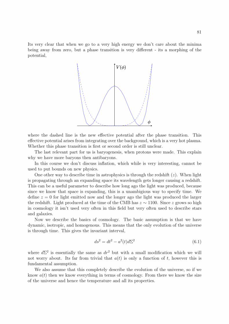
81
Its very clear that when we go to a very high energy we don’t care about the minimabeing away from zero, but a phase transition is very different - its a morphing of thepotential,
φ
V (φ)
φ
V (φ)
where the dashed line is the new effective potential after the phase transition. Thiseffective potential arises from integrating over the background, which is a very hot plasma.Whether this phase transition is first or second order is still unclear.
The last relevant part for us is baryogenesis, when protons were made. This explainwhy we have more baryons then antibaryons.
In this course we don’t discuss inflation, which while is very interesting, cannot beused to put bounds on new physics.
One other way to describe time in astrophysics is through the redshift (z). When lightis propagating through an expanding space its wavelength gets longer causing a redshift.This can be a useful parameter to describe how long ago the light was produced, becausesince we know that space is expanding, this is a unambigious way to specify time. Wedefine z = 0 for light emitted now and the longer ago the light was produced the largerthe redshift. Light produced at the time of the CMB has z ∼ 1100. Since z grows so highin cosmology it isn’t used very often in this field but very often used to describe starsand galaxies.
Now we describe the basics of cosmology. The basic assumption is that we havedynamic, isotropic, and homogenous. This means that the only evolution of the universeis through time. This gives the invariant interval,
ds2 = dt2 − a2(t)dΣ2 (6.1)
where dΣ2 is essentially the same as dr2 but with a small modification which we willnot worry about. Its far from trivial that a(t) is only a function of t, however this isfundamental assumption.
We also assume that this completely describe the evolution of the universe, so if weknow a(t) then we know everything in terms of cosmology. From there we know the sizeof the universe and hence the temperature and all its properties.
82 CHAPTER 6. COSMOLOGY
This a(t) is related to the redshift and the wavelength of light emitted at time t (λ(t))by,
1 + z ≡ a(t0)
a(t)=λ(t0)
λ(t)(6.2)
We define the Hubble constant,
H(t) =a(t)
a(t)(6.3)
This is not a constant in time, but in direction. H tells you how fast the universe ischanging. H tells you the typical time scale for things that happen in the universe.When we talk about cosmology, each process has some time, e.g. a neutron decaying.When we talk about BBN we can compare the neutron decay rate (15min) to the Hubbleconstant. If Γneutron H then we can treat the neutron as stable.
The current value of H is,H0 ∼ 10−33eV (6.4)
This is a very small number compared to quantities we are used to in particle physics.Thus we almost never have to worry about the effects of this expansion. Taking theinverse of this quantity give the lifetime of the universe, ∼ 13.7 billion years.
The Hubble law says that,H0d ≈ z (z 1) (6.5)
where d is the distance to a given object.[Q 34: Derive this]In order to solve a(t) we need to solve Einstein’s equations which are related to the
matter in the universe. We define the critical density of the universe as,
ρc ≡3H2
0
8πGN
(6.6)
This is the density that the universe would have collapsed (there is so much mass that itwill implode).
Furthermore we define,
Ωi =ρiρc
(6.7)
For example ΩDM ∼ 0.23. In general one wouldn’t expect ρi to have anything to do withρc. However, it turns that that
∑i ρi ≈ ρc. This is a very important piece of evidence
for inflation (though its not trivial why this is the case).We can separate the different densities through,
Ω = Ωmatter + ΩDM + ΩCC (6.8)
How the universe expands depends on what particles are inside it. If we have a boxwith a gas of a certain density and we increase the length of each side of the box by 2,then the density will go down by a factor of 23. So we see that for regular matter,
ρ ∝ L−3 (6.9)
83
where L is the length of the sides of the box. For the universe the length of the box isessentially given by a. Therefore we have,
ρ ∝ a−3 (6.10)
For photons the same reduction in number density will happen. However, here the energyof the photons will change when we increase the size of the box due to the redshift.Therefore, we have,1
ρ ∝ a−4 (6.11)
The cosmological constant doesn’t change with scale. So we have,
ρCC = a0 (6.12)
This is very peculiar. For radiation and for the cosmological constant, the energy of theuniverse changes when we increase the size of the universe. Therefore, in this case wedon’t have energy conservation. This is because energy conservation is a consequence oftime translation invariance. However, we don’t have this symmetry here since we haveexpansion so we don’t have energy conservation!
We can get these relationships from the equation of state which relates the density tothe pressure in the universe,
p = wρ (6.13)
where w is a constant. For matter w = 0. For radiation, w = 1/3, and for the cosmologicalconstant, w = −1. [Q 35: Derive these from thermo.] This gives,
ρ ∼ a−3(1+w) (6.14)
So knowing how the density scales with a is the same as knowing w.From here you can find how a(t) is dependent on time,
a = t2/(3(1+w)) (6.15)
It isn’t trivial that we can define a temperature for the universe. This is becausetypical definitions of temperature require things to be in equilibrium.
Lets think how the number density of electrons scales with temperatures. If thetemperature is below the electron mass, then it is a constant. On the other hand, thenumber density of photons always scales with the temperature, nγ ∝ T 3 and so ργ ∝ T 4,since they never become non-relativistic.
Suppose we are in the radiation dominated era of cosmology. Then we have the energydensity of radiation,
ρR =π2
30g∗T
4 (6.16)
1This is easy to see from thermodynamics,
ρ ∼∫dp
p3
ep/T + 1∼ T 4
84 CHAPTER 6. COSMOLOGY
where g∗ is the effective number of degrees of freedom, g∗ = gB + 7gF/8, and gB, gF arethe number of degrees of freedom of bosons and fermions. You can kind of understandwhy the fermions are less important then the bosons. You can’t put two fermions in asingle level, so you can’t place them close together which makes you have a hard time toincrease the density. g∗ changes as a function of time, but it changes very slowly.
Say we start with a radiation dominated universe. Since ρrad ∝ a−4 and ρmat ∝ a−3
the universe will at one point become matter dominated instead.In general we think of the evolution of the universe as,
ΩCC → Ωrad → Ωmat → ΩCC (6.17)
In general Ωi is equal to 1 for a single type of energy at one point in time. Transitionsperiods are very short. Baryogensis for example, occurs in the radiation dominant era.
Right now we are in between matter domination and cosmological constant domina-tion. It is peculiar that we live in this special time that we are in between two regions.This is an unsolved problem of cosmology. [Q 36: Draw the different density curves.]
Currently we say that the temperature of the universe is 2.7 K. This means that thephotons from the big bang at 2.7 K (as opposed to e.g. the neutrinos).
Through more algebra one can show that,
H(T ) = T 2√g∗(
7π3GN
90
)1/2
(6.18)
The very last definition that we have is the entropy density,
S =ρ+ p
T=
2π2
4πg∗T
3 (6.19)
As of today the number density of photons is related to the entropy by,
S ' 7nγ (6.20)
The number density also scales like T 3 so we often use these interchangeably.Decoupling or “freezing out” is the last important topic we need to understand. Say
you have a universe with a plasma and a particle A with temperature, T mA wheremA is the mass of the particle. The particle will contantly interact with its surroundings(i.e., in equilibrium). This is independent of the details of the plasma, but just requiresthat the cross section of interaction will be large compared to how fast the universe isexpanding. In this case the number density goes as, nA ∼ T 3e−mA/T . If mA T thenthe exponential is harmless and e−mA/T ∼ 1. However, if mA ∼ T then the exponentialbecomes important the number density sharply drops.
However, this is not the end of the story. At one point the particles interaction crosssection will become so low that it effectively doesn’t interact with the thermal bath at all.At what point this will occur isn’t obvious but usually will occur at some point T mA.The larger the interaction cross section is (relative to the mass) the longer the particlewill remain in thermal equilibrium and hence be exponentially suppressed. This is shownbelow:
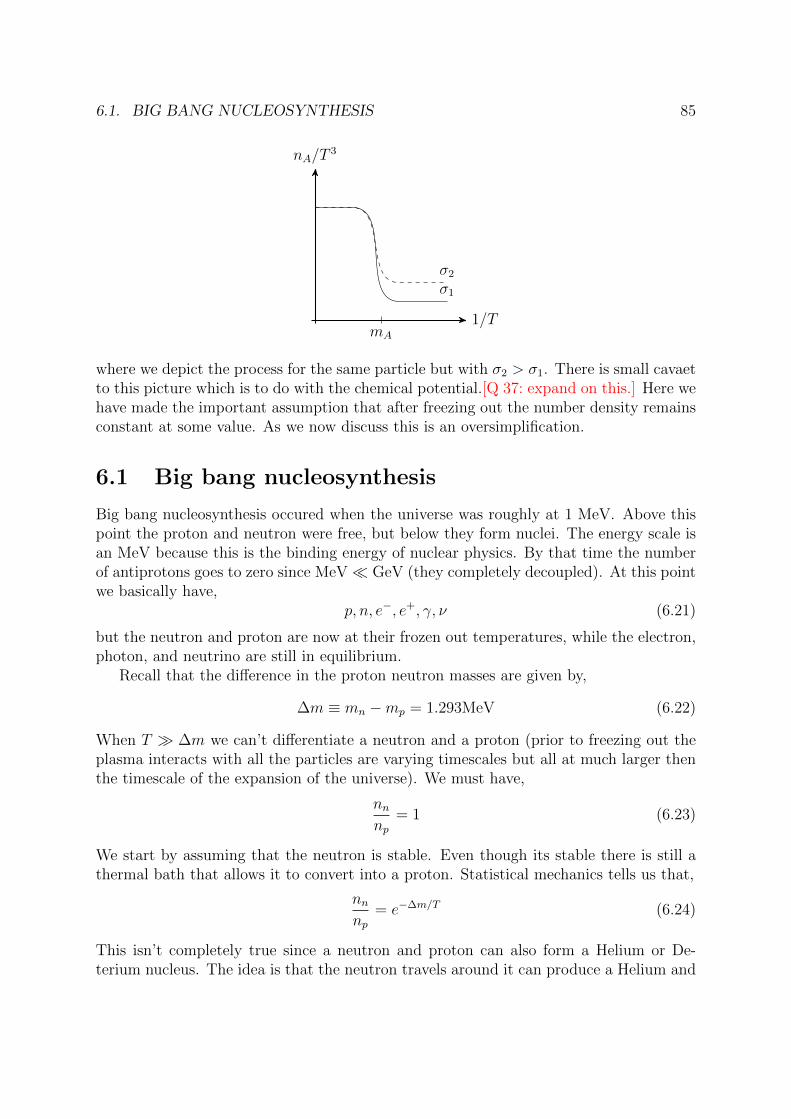
6.1. BIG BANG NUCLEOSYNTHESIS 85
nA/T3
1/T
σ1
σ2
mA
where we depict the process for the same particle but with σ2 > σ1. There is small cavaetto this picture which is to do with the chemical potential.[Q 37: expand on this.] Here wehave made the important assumption that after freezing out the number density remainsconstant at some value. As we now discuss this is an oversimplification.
6.1 Big bang nucleosynthesis
Big bang nucleosynthesis occured when the universe was roughly at 1 MeV. Above thispoint the proton and neutron were free, but below they form nuclei. The energy scale isan MeV because this is the binding energy of nuclear physics. By that time the numberof antiprotons goes to zero since MeV GeV (they completely decoupled). At this pointwe basically have,
p, n, e−, e+, γ, ν (6.21)
but the neutron and proton are now at their frozen out temperatures, while the electron,photon, and neutrino are still in equilibrium.
Recall that the difference in the proton neutron masses are given by,
∆m ≡ mn −mp = 1.293MeV (6.22)
When T ∆m we can’t differentiate a neutron and a proton (prior to freezing out theplasma interacts with all the particles are varying timescales but all at much larger thenthe timescale of the expansion of the universe). We must have,
nnnp
= 1 (6.23)
We start by assuming that the neutron is stable. Even though its stable there is still athermal bath that allows it to convert into a proton. Statistical mechanics tells us that,
nnnp
= e−∆m/T (6.24)
This isn’t completely true since a neutron and proton can also form a Helium or De-terium nucleus. The idea is that the neutron travels around it can produce a Helium and
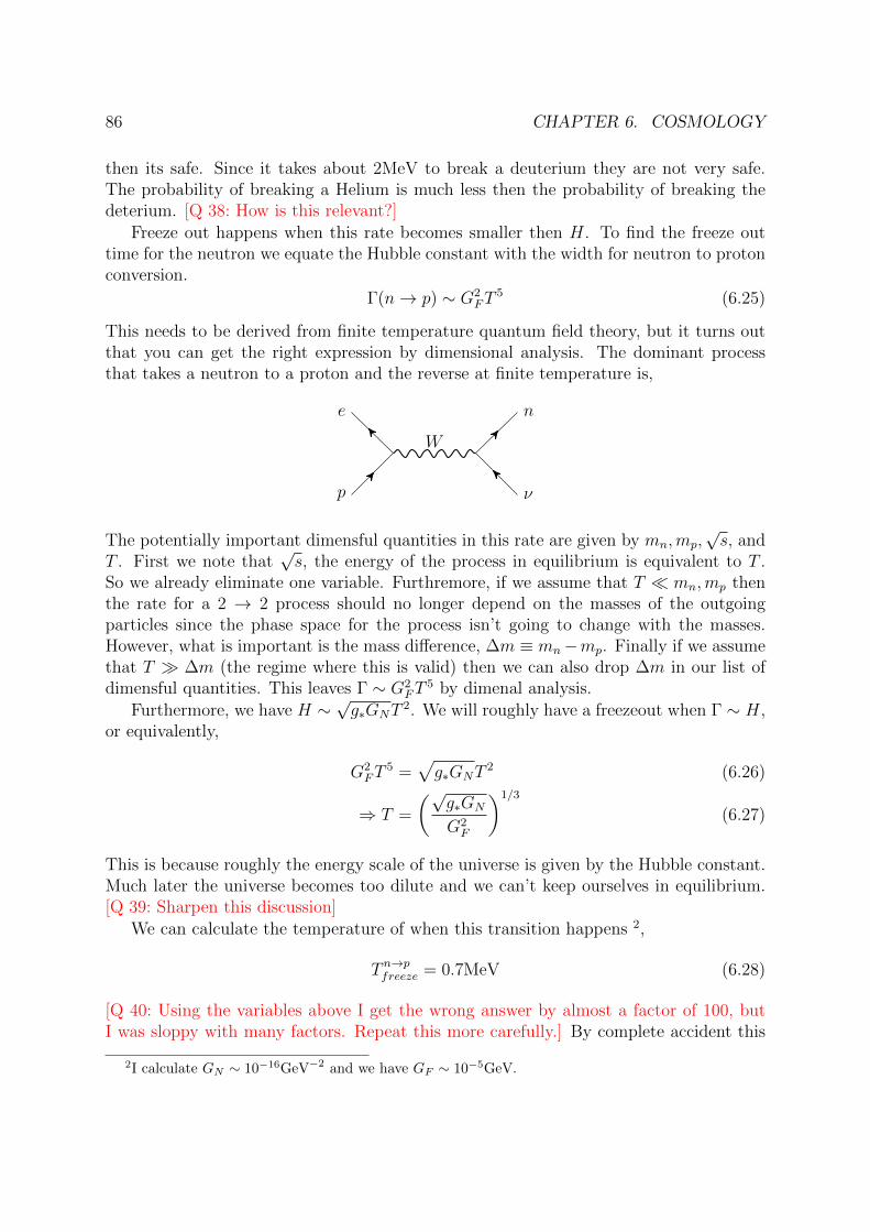
86 CHAPTER 6. COSMOLOGY
then its safe. Since it takes about 2MeV to break a deuterium they are not very safe.The probability of breaking a Helium is much less then the probability of breaking thedeterium. [Q 38: How is this relevant?]
Freeze out happens when this rate becomes smaller then H. To find the freeze outtime for the neutron we equate the Hubble constant with the width for neutron to protonconversion.
Γ(n→ p) ∼ G2FT
5 (6.25)
This needs to be derived from finite temperature quantum field theory, but it turns outthat you can get the right expression by dimensional analysis. The dominant processthat takes a neutron to a proton and the reverse at finite temperature is,
p
e
W
n
ν
The potentially important dimensful quantities in this rate are given by mn,mp,√s, and
T . First we note that√s, the energy of the process in equilibrium is equivalent to T .
So we already eliminate one variable. Furthremore, if we assume that T mn,mp thenthe rate for a 2 → 2 process should no longer depend on the masses of the outgoingparticles since the phase space for the process isn’t going to change with the masses.However, what is important is the mass difference, ∆m ≡ mn−mp. Finally if we assumethat T ∆m (the regime where this is valid) then we can also drop ∆m in our list ofdimensful quantities. This leaves Γ ∼ G2
FT5 by dimenal analysis.
Furthermore, we have H ∼√g∗GNT
2. We will roughly have a freezeout when Γ ∼ H,or equivalently,
G2FT
5 =√g∗GNT
2 (6.26)
⇒ T =
(√g∗GN
G2F
)1/3
(6.27)
This is because roughly the energy scale of the universe is given by the Hubble constant.Much later the universe becomes too dilute and we can’t keep ourselves in equilibrium.[Q 39: Sharpen this discussion]
We can calculate the temperature of when this transition happens 2,
T n→pfreeze = 0.7MeV (6.28)
[Q 40: Using the variables above I get the wrong answer by almost a factor of 100, butI was sloppy with many factors. Repeat this more carefully.] By complete accident this
2I calculate GN ∼ 10−16GeV−2 and we have GF ∼ 10−5GeV.
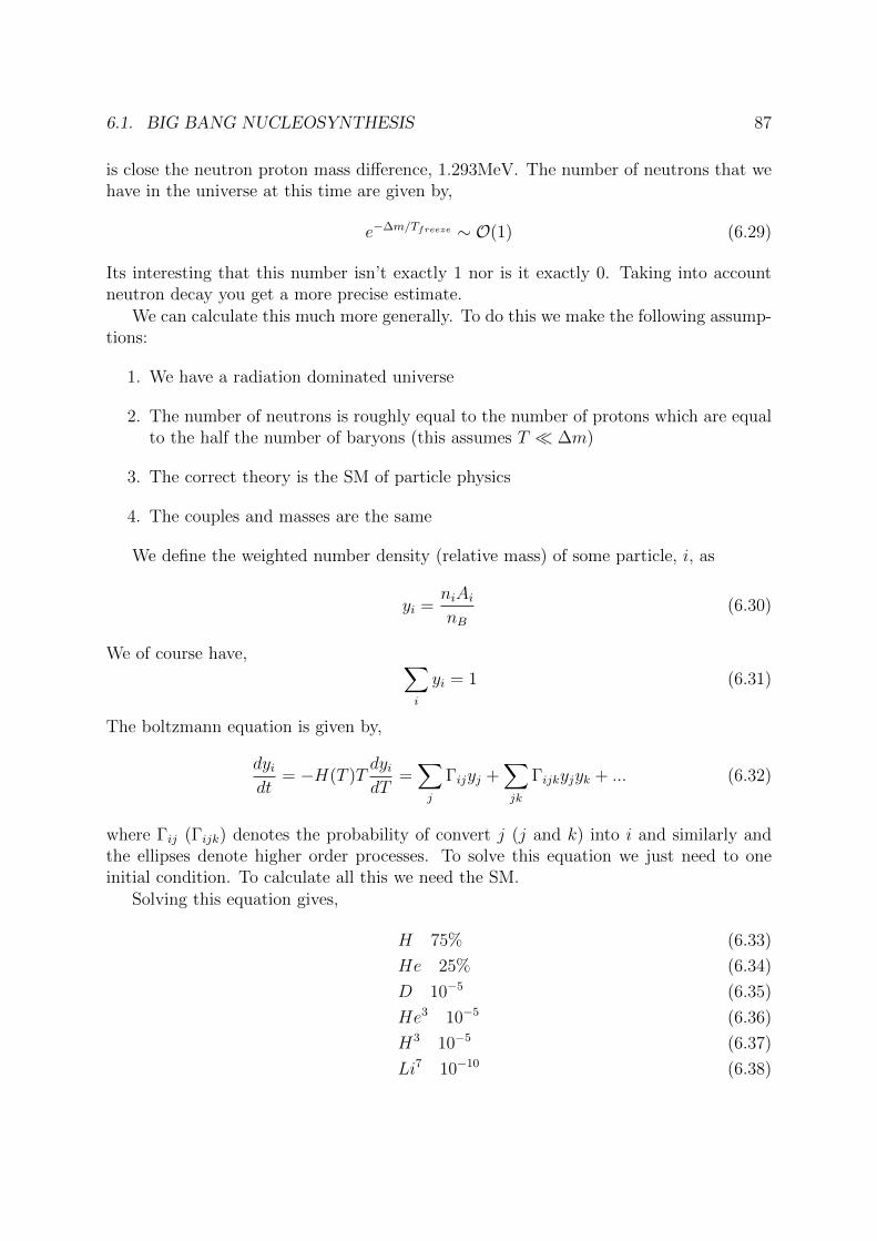
6.1. BIG BANG NUCLEOSYNTHESIS 87
is close the neutron proton mass difference, 1.293MeV. The number of neutrons that wehave in the universe at this time are given by,
e−∆m/Tfreeze ∼ O(1) (6.29)
Its interesting that this number isn’t exactly 1 nor is it exactly 0. Taking into accountneutron decay you get a more precise estimate.
We can calculate this much more generally. To do this we make the following assump-tions:
1. We have a radiation dominated universe
2. The number of neutrons is roughly equal to the number of protons which are equalto the half the number of baryons (this assumes T ∆m)
3. The correct theory is the SM of particle physics
4. The couples and masses are the same
We define the weighted number density (relative mass) of some particle, i, as
yi =niAinB
(6.30)
We of course have, ∑i
yi = 1 (6.31)
The boltzmann equation is given by,
dyidt
= −H(T )TdyidT
=∑j
Γijyj +∑jk
Γijkyjyk + ... (6.32)
where Γij (Γijk) denotes the probability of convert j (j and k) into i and similarly andthe ellipses denote higher order processes. To solve this equation we just need to oneinitial condition. To calculate all this we need the SM.
Solving this equation gives,
H 75% (6.33)
He 25% (6.34)
D 10−5 (6.35)
He3 10−5 (6.36)
H3 10−5 (6.37)
Li7 10−10 (6.38)
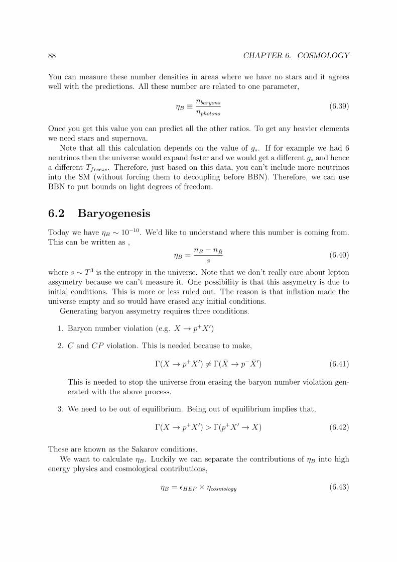
88 CHAPTER 6. COSMOLOGY
You can measure these number densities in areas where we have no stars and it agreeswell with the predictions. All these number are related to one parameter,
ηB ≡nbaryonsnphotons
(6.39)
Once you get this value you can predict all the other ratios. To get any heavier elementswe need stars and supernova.
Note that all this calculation depends on the value of g∗. If for example we had 6neutrinos then the universe would expand faster and we would get a different g∗ and hencea different Tfreeze. Therefore, just based on this data, you can’t include more neutrinosinto the SM (without forcing them to decoupling before BBN). Therefore, we can useBBN to put bounds on light degrees of freedom.
6.2 Baryogenesis
Today we have ηB ∼ 10−10. We’d like to understand where this number is coming from.This can be written as ,
ηB =nB − nB
s(6.40)
where s ∼ T 3 is the entropy in the universe. Note that we don’t really care about leptonassymetry because we can’t measure it. One possibility is that this assymetry is due toinitial conditions. This is more or less ruled out. The reason is that inflation made theuniverse empty and so would have erased any initial conditions.
Generating baryon assymetry requires three conditions.
1. Baryon number violation (e.g. X → p+X ′)
2. C and CP violation. This is needed because to make,
Γ(X → p+X ′) 6= Γ(X → p−X ′) (6.41)
This is needed to stop the universe from erasing the baryon number violation gen-erated with the above process.
3. We need to be out of equilibrium. Being out of equilibrium implies that,
Γ(X → p+X ′) > Γ(p+X ′ → X) (6.42)
These are known as the Sakarov conditions.We want to calculate ηB. Luckily we can separate the contributions of ηB into high
energy physics and cosmological contributions,
ηB = εHEP × ηcosmology (6.43)
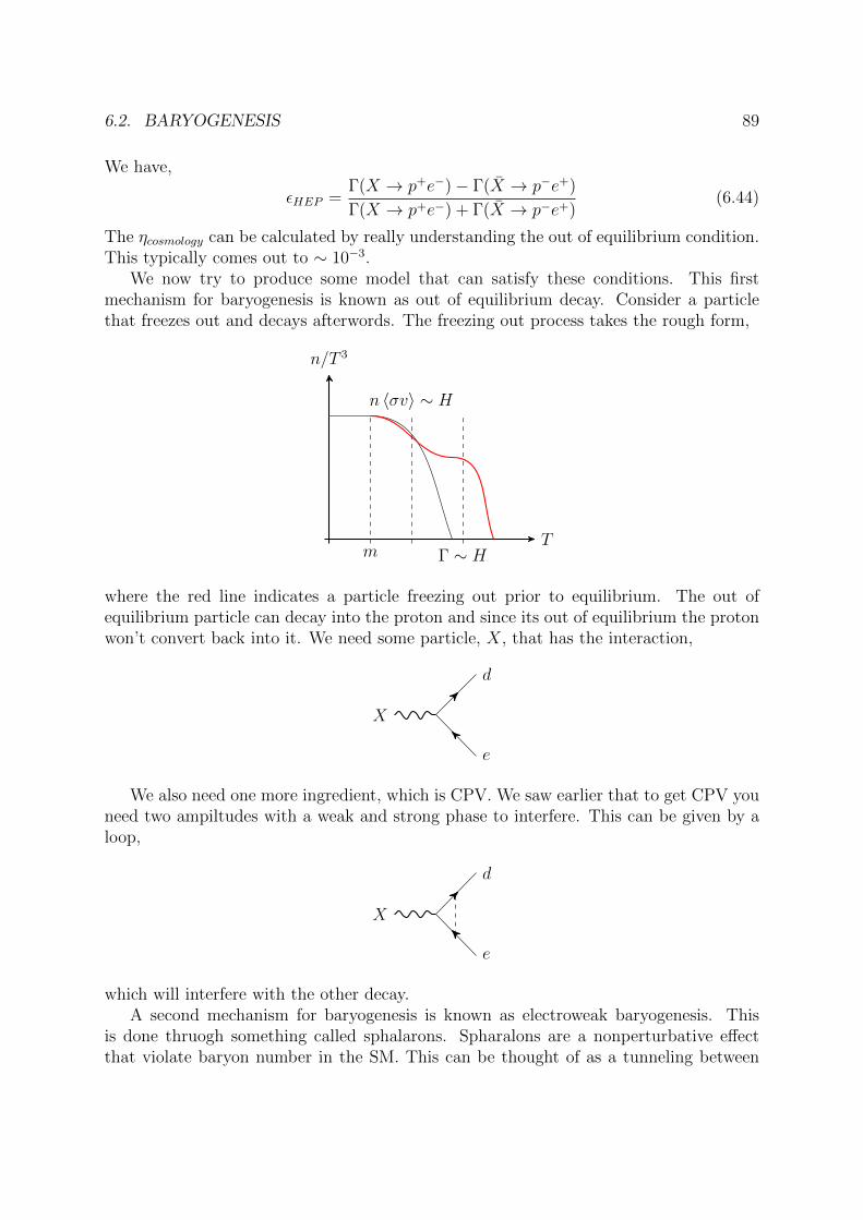
6.2. BARYOGENESIS 89
We have,
εHEP =Γ(X → p+e−)− Γ(X → p−e+)
Γ(X → p+e−) + Γ(X → p−e+)(6.44)
The ηcosmology can be calculated by really understanding the out of equilibrium condition.This typically comes out to ∼ 10−3.
We now try to produce some model that can satisfy these conditions. This firstmechanism for baryogenesis is known as out of equilibrium decay. Consider a particlethat freezes out and decays afterwords. The freezing out process takes the rough form,
n/T 3
Tm
n 〈σv〉 ∼ H
Γ ∼ H
where the red line indicates a particle freezing out prior to equilibrium. The out ofequilibrium particle can decay into the proton and since its out of equilibrium the protonwon’t convert back into it. We need some particle, X, that has the interaction,
X
d
e
We also need one more ingredient, which is CPV. We saw earlier that to get CPV youneed two ampiltudes with a weak and strong phase to interfere. This can be given by aloop,
X
d
e
which will interfere with the other decay.A second mechanism for baryogenesis is known as electroweak baryogenesis. This
is done thruogh something called sphalarons. Spharalons are a nonperturbative effectthat violate baryon number in the SM. This can be thought of as a tunneling between
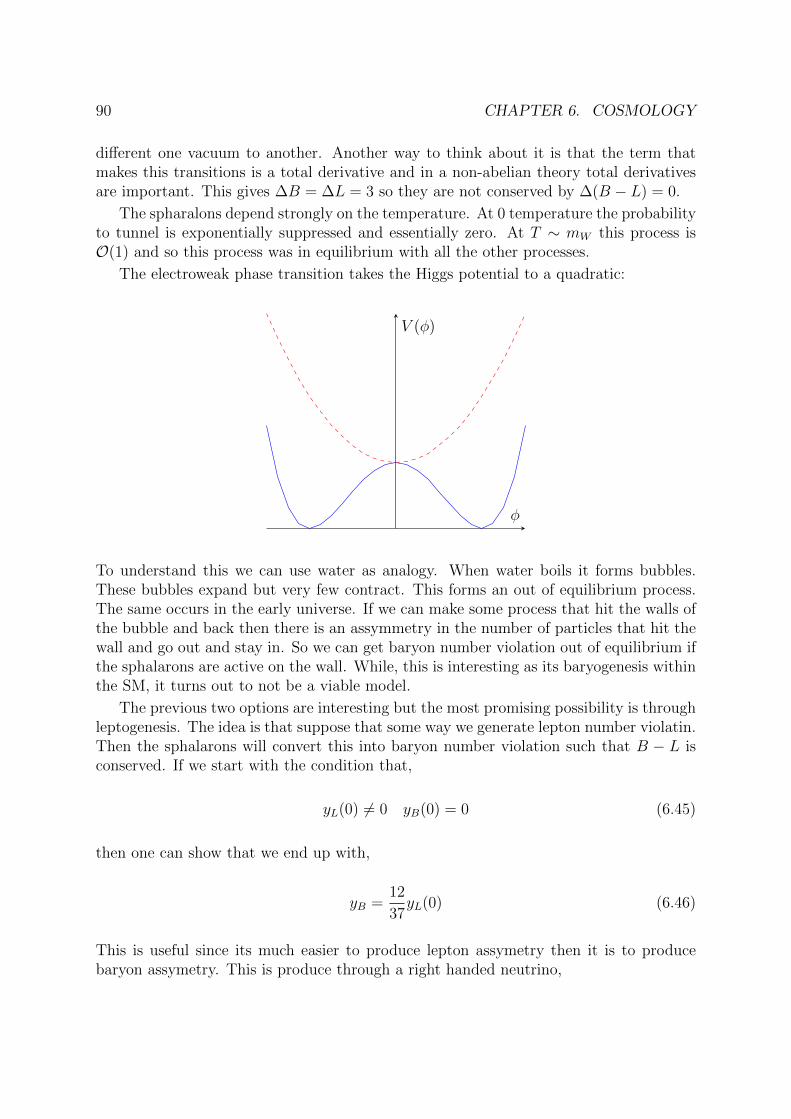
90 CHAPTER 6. COSMOLOGY
different one vacuum to another. Another way to think about it is that the term thatmakes this transitions is a total derivative and in a non-abelian theory total derivativesare important. This gives ∆B = ∆L = 3 so they are not conserved by ∆(B − L) = 0.
The spharalons depend strongly on the temperature. At 0 temperature the probabilityto tunnel is exponentially suppressed and essentially zero. At T ∼ mW this process isO(1) and so this process was in equilibrium with all the other processes.
The electroweak phase transition takes the Higgs potential to a quadratic:
φ
V (φ)
To understand this we can use water as analogy. When water boils it forms bubbles.These bubbles expand but very few contract. This forms an out of equilibrium process.The same occurs in the early universe. If we can make some process that hit the walls ofthe bubble and back then there is an assymmetry in the number of particles that hit thewall and go out and stay in. So we can get baryon number violation out of equilibrium ifthe sphalarons are active on the wall. While, this is interesting as its baryogenesis withinthe SM, it turns out to not be a viable model.
The previous two options are interesting but the most promising possibility is throughleptogenesis. The idea is that suppose that some way we generate lepton number violatin.Then the sphalarons will convert this into baryon number violation such that B − L isconserved. If we start with the condition that,
yL(0) 6= 0 yB(0) = 0 (6.45)
then one can show that we end up with,
yB =12
37yL(0) (6.46)
This is useful since its much easier to produce lepton assymetry then it is to producebaryon assymetry. This is produce through a right handed neutrino,
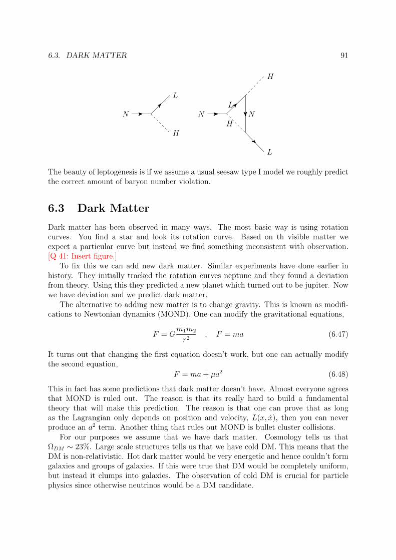
6.3. DARK MATTER 91
N
L
H
NL
H
L
N
H
The beauty of leptogenesis is if we assume a usual seesaw type I model we roughly predictthe correct amount of baryon number violation.
6.3 Dark Matter
Dark matter has been observed in many ways. The most basic way is using rotationcurves. You find a star and look its rotation curve. Based on th visible matter weexpect a particular curve but instead we find something inconsistent with observation.[Q 41: Insert figure.]
To fix this we can add new dark matter. Similar experiments have done earlier inhistory. They initially tracked the rotation curves neptune and they found a deviationfrom theory. Using this they predicted a new planet which turned out to be jupiter. Nowwe have deviation and we predict dark matter.
The alternative to adding new matter is to change gravity. This is known as modifi-cations to Newtonian dynamics (MOND). One can modify the gravitational equations,
F = Gm1m2
r2, F = ma (6.47)
It turns out that changing the first equation doesn’t work, but one can actually modifythe second equation,
F = ma+ µa2 (6.48)
This in fact has some predictions that dark matter doesn’t have. Almost everyone agreesthat MOND is ruled out. The reason is that its really hard to build a fundamentaltheory that will make this prediction. The reason is that one can prove that as longas the Lagrangian only depends on position and velocity, L(x, x), then you can neverproduce an a2 term. Another thing that rules out MOND is bullet cluster collisions.
For our purposes we assume that we have dark matter. Cosmology tells us thatΩDM ∼ 23%. Large scale structures tells us that we have cold DM. This means that theDM is non-relativistic. Hot dark matter would be very energetic and hence couldn’t formgalaxies and groups of galaxies. If this were true that DM would be completely uniform,but instead it clumps into galaxies. The observation of cold DM is crucial for particlephysics since otherwise neutrinos would be a DM candidate.
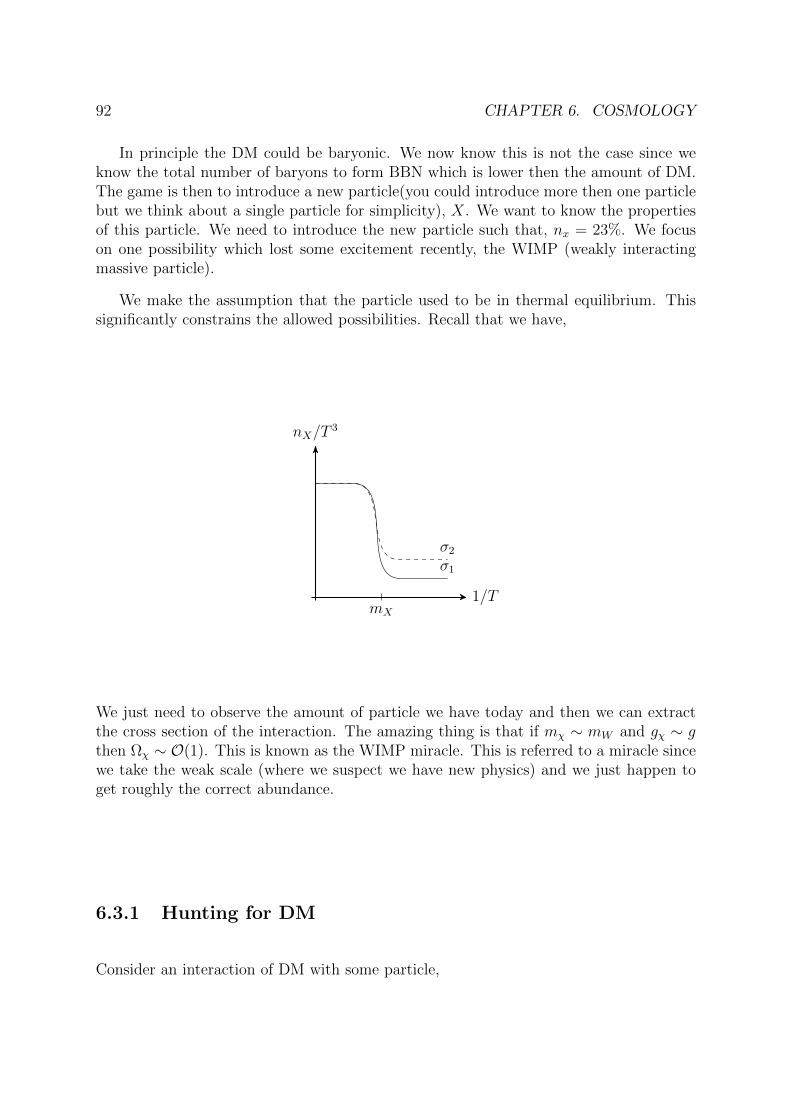
92 CHAPTER 6. COSMOLOGY
In principle the DM could be baryonic. We now know this is not the case since weknow the total number of baryons to form BBN which is lower then the amount of DM.The game is then to introduce a new particle(you could introduce more then one particlebut we think about a single particle for simplicity), X. We want to know the propertiesof this particle. We need to introduce the new particle such that, nx = 23%. We focuson one possibility which lost some excitement recently, the WIMP (weakly interactingmassive particle).
We make the assumption that the particle used to be in thermal equilibrium. Thissignificantly constrains the allowed possibilities. Recall that we have,
nX/T3
1/T
σ1
σ2
mX
We just need to observe the amount of particle we have today and then we can extractthe cross section of the interaction. The amazing thing is that if mχ ∼ mW and gχ ∼ gthen Ωχ ∼ O(1). This is known as the WIMP miracle. This is referred to a miracle sincewe take the weak scale (where we suspect we have new physics) and we just happen toget roughly the correct abundance.
6.3.1 Hunting for DM
Consider an interaction of DM with some particle,
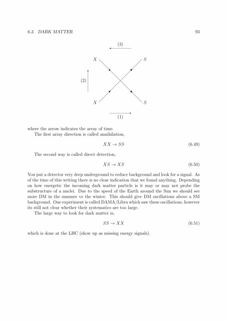
6.3. DARK MATTER 93
X
X S
S
(1)
(2)
(3)
where the arrow indicates the array of time.The first array direction is called annihilation,
XX → SS (6.49)
The second way is called direct detection,
XS → XS (6.50)
You put a detector very deep underground to reduce background and look for a signal. Asof the time of this writing there is no clear indication that we found anything. Dependingon how energetic the incoming dark matter particle is it may or may not probe thesubstructure of a nuclei. Due to the speed of the Earth around the Sun we should seemore DM in the summer vs the winter. This should give DM oscillations above a SMbackground. One experiment is called DAMA/Libra which saw these oscillations, howeverits still not clear whether their systematics are too large.
The large way to look for dark matter is,
SS → XX (6.51)
which is done at the LHC (show up as missing energy signals).
Chapter 7
Grand Unified Theories
7.1 Introduction
In this chapter we describe grand unified theories in detail. Unlike the rest of the bookthis chapter is made using a compilation of references including the lectures by YuvalGrossman, a set of 3 lectures by Stuart Raby at PITP on SUSY GUTs, and Supersym-metry - Theory,Experiment, and Cosmology by Pierre Binetruy.
Unification is the bringing together of symmetry groups into a fewer groups. Elec-troweak unification is an example of this, where we can describe weak and electromagneticphysics using the group group, SU(2) × U(1). Grand unified theories (GUTs) are onesthat try to unify the strong force as well.
The zeroth order motivation for GUTs is that when we run all 3 gauge couplings tohigher energies with our current field content we find that they all meet at roughly thesame energy scale.
Other motivations are the correct predictions of the Weinberg angle as well as therelative values of the bottom and tau Yukawa. The final important motivation for GUTsis charge quantization. In general the changes of all the particles could be completelyarbitrary. This is because charges of Abelian symmetries are continuous. However, inNature we see a very strange pattern between the charges. In particular they are allmultiples of some fundamental charge. GUTs fix this because the charges come from anon-abelian symmetry. Non-abelian symmetries have quantized charges (e.g. the T3 ofall lepton and quark doublets can’t be continuous but are fixed to be ±1/2).
GUTs can also help with other SM puzzles such as neutrino masses, baryogenesis, aswell as flavor.
The striking prediction of all GUTs is proton decay. The reason for this is that grandunified theories put lepton and quarks in the same multiplets. This breaks lepton andbaryon number explicitly. Proton decay experiments are ongoing. The most common issuperK, which is now commonly used as a neutrino machine instead.
94
7.2. A LITTLE GROUP THEORY 95
7.2 A little group theory
We want to consider the breaking of a Lie group into the SM Lie groups. This is a highlynontrivial process and apriori its not obvious how a group will break under spontaneoussymmetry breaking. In order to find the breaking patterns without resorting to repre-sentations we can use the technique known as Dynkin diagrams. This is very simple toimplement but confusing to justify.
[Q 42: Expand on this section and fix the reference...]One strong indication that the SM arises from a larger gauge group is that the SM
matter fields all add to zero. To see why this is important we recall that non-abeliangroup generators must be traceless. Furthermore, for hypercharge to be unbroken afterthe breaking of the gauge group, it must form a subgroup of the GUT group and henceappear as one of the GUT generators (in some choice of basis). Explicitly this says thatif we denote the particles in representation n by |in〉 then we must have,
〈in|Y |jn〉 = δinjnyjn (7.1)
where Y denotes the hypercharge generator in the GUT group. However, if the SM fieldsmake up a collection of complete representations (no new fields) then we have,∑
n
∑in
〈in|Y |in〉 =∑n
∑in
yn,in = 0 (7.2)
where the sum on the right is just sums over all particles in all representations. For theSM fields we have,∑
n,in
yn,in =
(−1
2− 1
2− 1 + 3
(1
6+
1
6+
2
3− 1
3
))× 3 = 0 (7.3)
as required. This also shows that one cannot include the Higgs field into the GUT groupsince doing so wouldn’t allow hypercharge to be unbroken after breaking the GUT groupunless one includes other new fields as well.
7.3 Coupling Unification
There are two ways to proceed to see if coupling constant unify. We could either start inthe IR and run the couplings up to the GUT scale or we could start in the UV and thenrun the couplings down to scale of experiment. Here we proceed in the first way.
The running of couplings takes the form1,
dα
d log µ= −bi
α2
2π, bi =
(11
3C2(G)− 2
3C(r)nweyl −
1
3C(r)nscalar
)(7.4)
1Note the factor of two difference in fermionic and bosonic results. This should be expected and isdue a Weyl fermion having two degrees of freedom.
96 CHAPTER 7. GRAND UNIFIED THEORIES
where µ is the renormalization scale, C2(G) = N for SU(N), C(r) = 12
for SU(N), nweylis the number of Weyl fermions, and nscalar is the number of complex scalars.
We have (as is common in discussions of GUTs we denote the gauge groups ofU(1)Y , SU(2)L, and SU(3)c as 1, 2, and 3 respectfully),
QCD : C2(G) = 3, C(r) = 1/2, nweyl = (
uR,dR,QL︷ ︸︸ ︷1 + 1 + 2)×Ng, nscalar = 0⇒ b3 = 7 (7.5)
SU(2)L : C2(G) = 2, C(r) = 1/2, nweyl = (
QL,L︷ ︸︸ ︷3 + 1)×Ng, nscalar = 1⇒ b2 =
19
6(7.6)
For hypercharge, due to its abelian nature the calculation is a bit different. In particular,the scale of hypercharge isn’t fixed as for non-abelian gauge theories. However, if weassume it will arise from the spontaneous breaking of some non-abelian group underwhich the SM fields from a full representation then it turns out that we can uniquelyrescale the hypercharge.
To see this we note that at the generators of the GUT group should all be normalizedin the same way, Tr
[T aT b
]= N
2δab. Explicitly we must have,∑
n
∑in
〈in|Y 2|in〉 =∑n
∑in
〈in|T3|in〉 (7.7)
Now since hypercharge doesn’t have a correct normalization in the SM case we can write,yα = CySM,α for particle α. Explicitly we have,∑
n
∑in
y2i,n =
∑n
∑in
t23,in (7.8)∑SM
C2y2SM =
∑SM
t23,SM (7.9)
where the sum is now over all the charges of the SM fields.Carrying out the sums we have,∑
SM
y2SM =
(1
4+
1
4+ 1 + 3×
(1
36+
1
36+ 1 +
4
9+
1
9
)3
)× 3 = 10 (7.10)
∑SM
t23,SM =
(1
4+
1
4+ 3×
(1
4+
1
4
))× 3 = 6 (7.11)
which gives,
C =
√10
6=
√5
3(7.12)
We see that when you go to the GUT scale the hypercharge is no longer arbitrary. It
is uniquely given by√
53
times the values which were conventionally assigned many years
ago. We will check this relationship again once we choose a particular GUT group.
7.3. COUPLING UNIFICATION 97
Alternatively one can think of scaling the couplings. To see this consider the La-grangians in the SM and the broken GUT. We must have,
LSM = g′YSMBµ (...) LGUT = gGUTY Bµ (...) (7.13)
i.e.
gGUTY = g′YSM = g′√
5
3Y (7.14)
which gives the relation,
gGUT =
√5
3g′ (7.15)
Now that we are equipped with this we are finally ready to consider the abelian aswell as non-abelian running. First we note that the one-loop coefficient for an abeliancoupling beta function is given by2,
b1 = − 1
C2
(2
3
∑f
y2f +
1
3y2φ
)⇒ bi = −41
10(7.16)
where yf and yφ are the SM gauge charges. This gives,
dα3
d log µ= −7
α23
2π(7.17)
dα2
d log µ= −19
6
α22
2π(7.18)
dα1
d log µ=
41
10
α21
2π(7.19)
The solution to the equation, α′ = βα2 is given by,
1
α=
1
α0
− β logµ
mZ
(7.20)
To track the couplings as a function of energy scale we need a starting point. Due toLEP these couplings are all best measured at the Z pole where they found,
α3(mZ) = 0.118 αe(mZ) = 1/128 sin2 θw(mZ) = 0.231 (7.21)
⇒α3(mZ) = 0.118 α2(mZ) = 0.0338 α1(mZ) = 0.0102× 5
3(7.22)
We can now plot the couplings as a function of energy. The result is shown below,
2To get the right results its important to note that above the EW scale the Higgs would count as twoscalars.
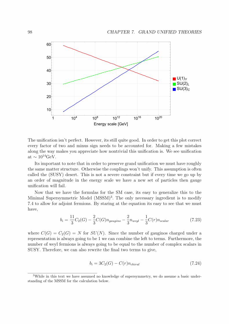
98 CHAPTER 7. GRAND UNIFIED THEORIES
1 104 108 1012 1016 1020
10
20
30
40
50
60
Energy scale [GeV]
1 U(1)YSU(2)LSU(3)C
The unification isn’t perfect. However, its still quite good. In order to get this plot correctevery factor of two and minus sign needs to be accounted for. Making a few mistakesalong the way makes you appreciate how nontrivial this unification is. We see unificationat ∼ 1014GeV.
Its important to note that in order to preserve grand unification we must have roughlythe same matter structure. Otherwise the couplings won’t unify. This assumption is oftencalled the (SUSY) desert. This is not a severe constraint but if every time we go up byan order of magnitude in the energy scale we have a new set of particles then gaugeunification will fail.
Now that we have the formulas for the SM case, its easy to generalize this to theMinimal Supersymmetric Model (MSSM)3. The only necessary ingredient is to modify7.4 to allow for adjoint fermions. By staring at the equation its easy to see that we musthave,
bi =11
3C2(G)− 2
3C(G)ngaugino −
2
3nweyl −
1
3C(r)nscalar (7.23)
where C(G) = C2(G) = N for SU(N). Since the number of gauginos charged under arepresentation is always going to be 1 we can combine the left to terms. Furthermore, thenumber of weyl fermions is always going to be equal to the number of complex scalars inSUSY. Therefore, we can also rewrite the final two terms to give,
bi = 3C2(G)− C(r)nchiral (7.24)
3While in this text we have assumed no knowledge of supersymmetry, we do assume a basic under-standing of the MSSM for the calculation below.
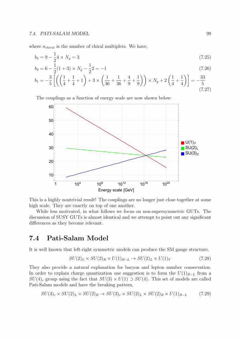
7.4. PATI-SALAM MODEL 99
where nchiral is the number of chiral multiplets. We have,
b3 = 9− 1
24×Ng = 3 (7.25)
b2 = 6− 1
2(1 + 3)×Ng −
1
22 = −1 (7.26)
b1 = −3
5
[((1
4+
1
4+ 1
)+ 3×
(1
36+
1
36+
4
9+
1
9
))×Ng + 2
(1
4+
1
4
)]= −33
5(7.27)
The couplings as a function of energy scale are now shown below:
1 104 108 1012 1016 1020
10
20
30
40
50
60
Energy scale [GeV]
U(1)YSU(2)LSU(3)C
This is a highly nontrivial result! The couplings are no longer just close together at somehigh scale. They are exactly on top of one another.
While less motivated, in what follows we focus on non-supersymmetric GUTs. Thediscussion of SUSY GUTs is almost identical and we attempt to point out any significantdifferences as they become relevant.
7.4 Pati-Salam Model
It is well known that left-right symmetric models can produce the SM gauge structure,
SU(2)L × SU(2)R × U(1)B−L → SU(2)L × U(1)Y (7.28)
They also provide a natural explanation for baryon and lepton number conservation.In order to explain charge quantization one suggestion is to form the U(1)B−L from aSU(4)c group using the fact that SU(3) × U(1) ⊃ SU(4). This set of models are calledPati-Salam models and have the breaking pattern,
SU(4)c × SU(2)L × SU(2)R → SU(3)c × SU(2)L × SU(2)R × U(1)B−L (7.29)
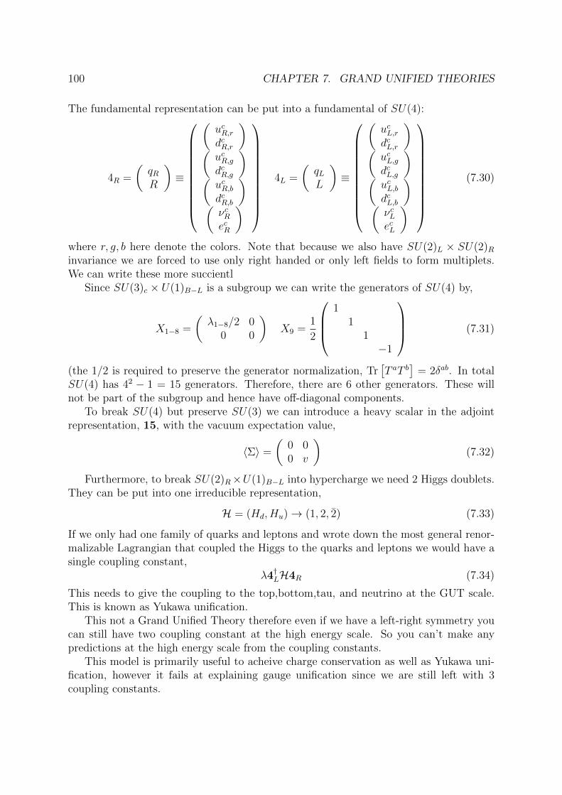
100 CHAPTER 7. GRAND UNIFIED THEORIES
The fundamental representation can be put into a fundamental of SU(4):
4R =
(qRR
)≡
(ucR,rdcR,r
)(ucR,gdcR,g
)(ucR,bdcR,b
)(νcRecR
)
4L =
(qLL
)≡
(ucL,rdcL,r
)(ucL,gdcL,g
)(ucL,bdcL,b
)(νcLecL
)
(7.30)
where r, g, b here denote the colors. Note that because we also have SU(2)L × SU(2)Rinvariance we are forced to use only right handed or only left fields to form multiplets.We can write these more succientl
Since SU(3)c × U(1)B−L is a subgroup we can write the generators of SU(4) by,
X1−8 =
(λ1−8/2 0
0 0
)X9 =
1
2
1
11−1
(7.31)
(the 1/2 is required to preserve the generator normalization, Tr[T aT b
]= 2δab. In total
SU(4) has 42 − 1 = 15 generators. Therefore, there are 6 other generators. These willnot be part of the subgroup and hence have off-diagonal components.
To break SU(4) but preserve SU(3) we can introduce a heavy scalar in the adjointrepresentation, 15, with the vacuum expectation value,
〈Σ〉 =
(0 00 v
)(7.32)
Furthermore, to break SU(2)R×U(1)B−L into hypercharge we need 2 Higgs doublets.They can be put into one irreducible representation,
H = (Hd, Hu)→ (1, 2, 2) (7.33)
If we only had one family of quarks and leptons and wrote down the most general renor-malizable Lagrangian that coupled the Higgs to the quarks and leptons we would have asingle coupling constant,
λ4†LH4R (7.34)
This needs to give the coupling to the top,bottom,tau, and neutrino at the GUT scale.This is known as Yukawa unification.
This not a Grand Unified Theory therefore even if we have a left-right symmetry youcan still have two coupling constant at the high energy scale. So you can’t make anypredictions at the high energy scale from the coupling constants.
This model is primarily useful to acheive charge conservation as well as Yukawa uni-fication, however it fails at explaining gauge unification since we are still left with 3coupling constants.
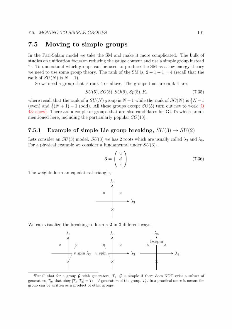
7.5. MOVING TO SIMPLE GROUPS 101
7.5 Moving to simple groups
In the Pati-Salam model we take the SM and make it more complicated. The bulk ofstudies on unification focus on reducing the gauge content and use a simple group instead4 . To understand which groups can be used to produce the SM as a low energy theorywe need to use some group theory. The rank of the SM is, 2 + 1 + 1 = 4 (recall that therank of SU(N) is N − 1).
So we need a group that is rank 4 or above. The groups that are rank 4 are:
SU(5), SO(8), SO(9), Sp(8), F4 (7.35)
where recall that the rank of a SU(N) group is N −1 while the rank of SO(N) is 12N −1
(even) and 12(N + 1)− 1 (odd). All these groups except SU(5) turn out not to work [Q
43: show]. There are a couple of groups that are also candidates for GUTs which aren’tmentioned here, including the particularly popular SO(10).
7.5.1 Example of simple Lie group breaking, SU(3)→ SU(2)
Lets consider an SU(3) model. SU(3) we has 2 roots which are usually called λ3 and λ8.For a physical example we consider a fundamental under SU(3)c,
3 =
uds
(7.36)
The weights form an equalateral triangle,
λ8
λ3
××
×
We can visualize the breaking to form a 2 in 3 different ways,
λ8
λ3
××
×
v spin
λ8
λ3
××
×
u spin
λ8
λ3
××
×
Isospin
4Recall that for a group G with generators, Tg, G is simple if there does NOT exist a subset ofgenerators, Th, that obey [Th, Tg] = Th ∀ generators of the group, Tg. In a practical sense it means thegroup can be written as a product of other groups.
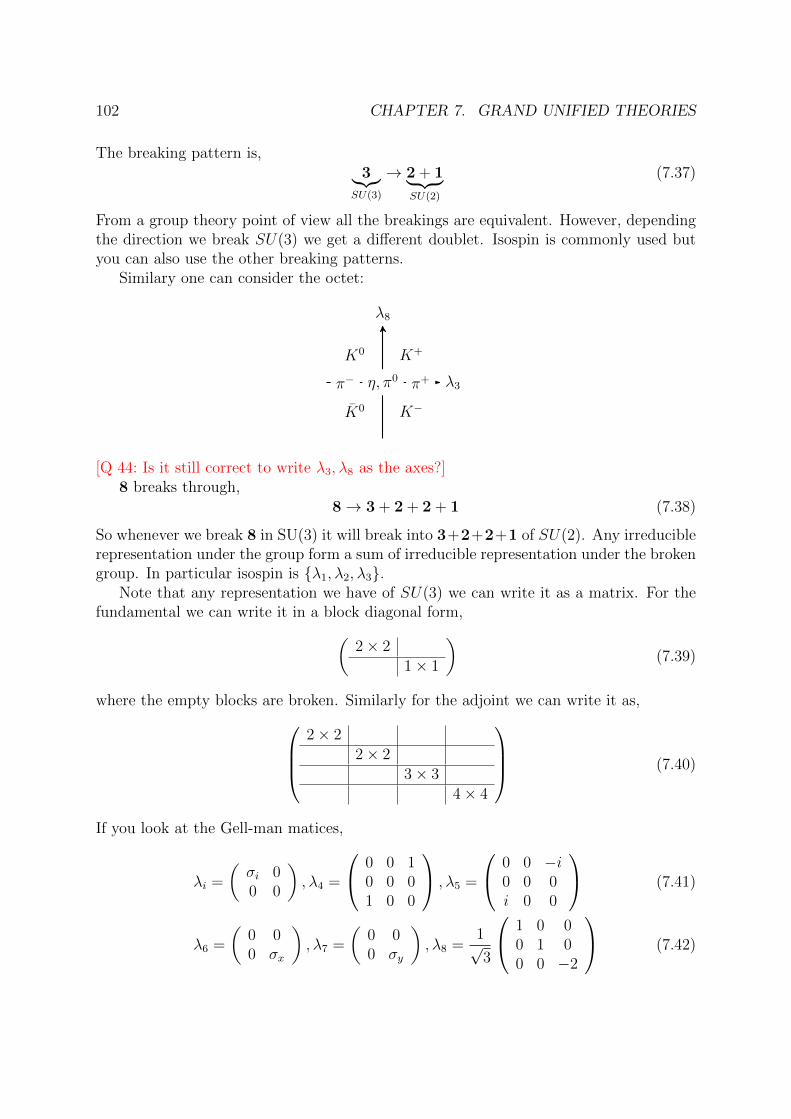
102 CHAPTER 7. GRAND UNIFIED THEORIES
The breaking pattern is,3︸︷︷︸
SU(3)
→ 2 + 1︸ ︷︷ ︸SU(2)
(7.37)
From a group theory point of view all the breakings are equivalent. However, dependingthe direction we break SU(3) we get a different doublet. Isospin is commonly used butyou can also use the other breaking patterns.
Similary one can consider the octet:
λ8
λ3
K+K0
K−K0
π+η, π0π−
[Q 44: Is it still correct to write λ3, λ8 as the axes?]8 breaks through,
8→ 3 + 2 + 2 + 1 (7.38)
So whenever we break 8 in SU(3) it will break into 3+2+2+1 of SU(2). Any irreduciblerepresentation under the group form a sum of irreducible representation under the brokengroup. In particular isospin is λ1, λ2, λ3.
Note that any representation we have of SU(3) we can write it as a matrix. For thefundamental we can write it in a block diagonal form,(
2× 21× 1
)(7.39)
where the empty blocks are broken. Similarly for the adjoint we can write it as,2× 2
2× 23× 3
4× 4
(7.40)
If you look at the Gell-man matices,
λi =
(σi 00 0
), λ4 =
0 0 10 0 01 0 0
, λ5 =
0 0 −i0 0 0i 0 0
(7.41)
λ6 =
(0 00 σx
), λ7 =
(0 00 σy
), λ8 =
1√3
1 0 00 1 00 0 −2
(7.42)
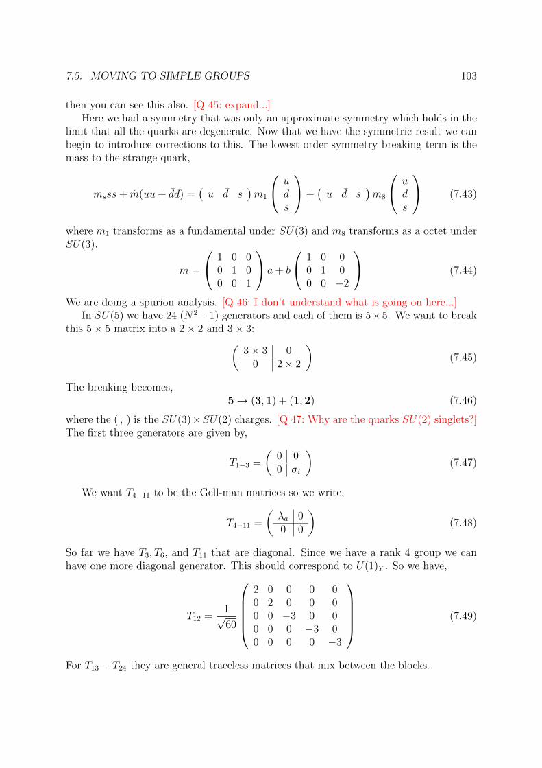
7.5. MOVING TO SIMPLE GROUPS 103
then you can see this also. [Q 45: expand...]Here we had a symmetry that was only an approximate symmetry which holds in the
limit that all the quarks are degenerate. Now that we have the symmetric result we canbegin to introduce corrections to this. The lowest order symmetry breaking term is themass to the strange quark,
msss+ m(uu+ dd) =(u d s
)m1
uds
+(u d s
)m8
uds
(7.43)
where m1 transforms as a fundamental under SU(3) and m8 transforms as a octet underSU(3).
m =
1 0 00 1 00 0 1
a+ b
1 0 00 1 00 0 −2
(7.44)
We are doing a spurion analysis. [Q 46: I don’t understand what is going on here...]In SU(5) we have 24 (N2−1) generators and each of them is 5×5. We want to break
this 5× 5 matrix into a 2× 2 and 3× 3:(3× 3 0
0 2× 2
)(7.45)
The breaking becomes,5→ (3,1) + (1,2) (7.46)
where the ( , ) is the SU(3)×SU(2) charges. [Q 47: Why are the quarks SU(2) singlets?]The first three generators are given by,
T1−3 =
(0 00 σi
)(7.47)
We want T4−11 to be the Gell-man matrices so we write,
T4−11 =
(λa 00 0
)(7.48)
So far we have T3, T6, and T11 that are diagonal. Since we have a rank 4 group we canhave one more diagonal generator. This should correspond to U(1)Y . So we have,
T12 =1√60
2 0 0 0 00 2 0 0 00 0 −3 0 00 0 0 −3 00 0 0 0 −3
(7.49)
For T13 − T24 they are general traceless matrices that mix between the blocks.
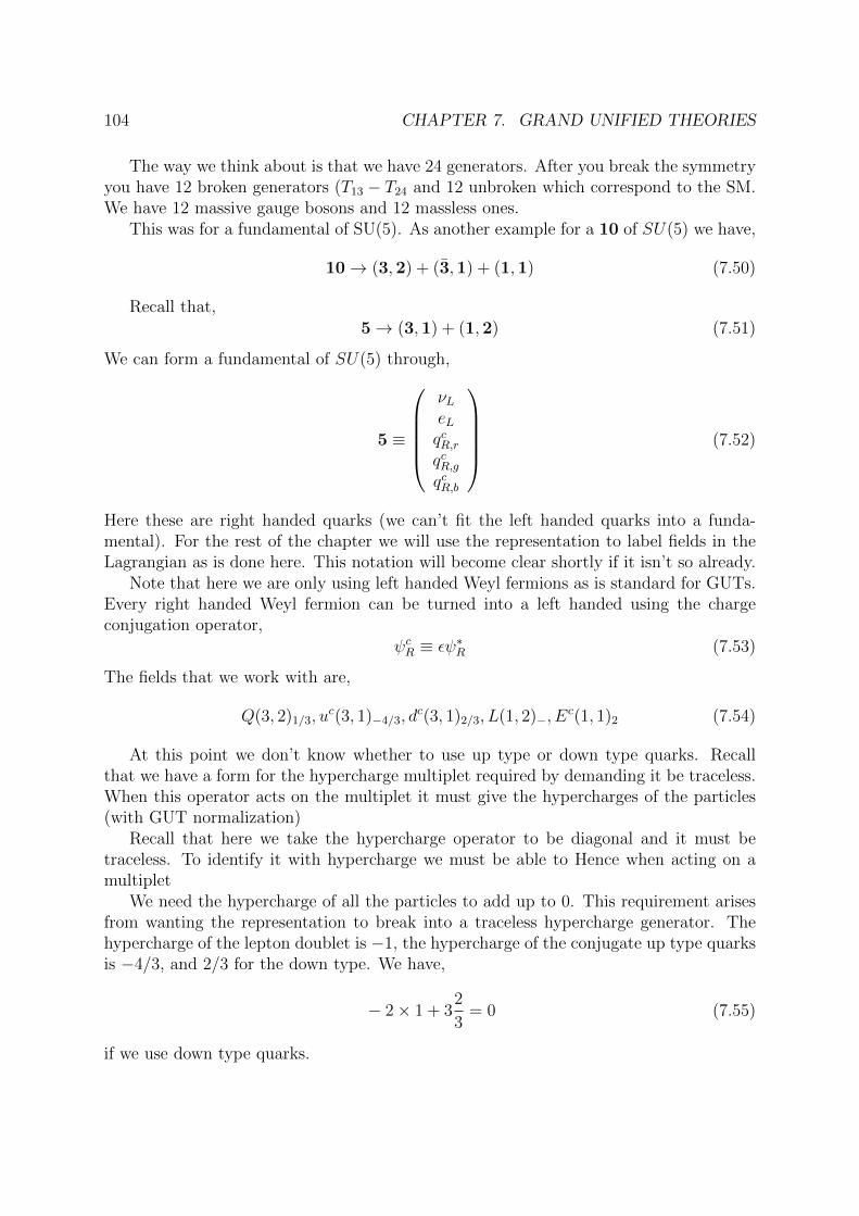
104 CHAPTER 7. GRAND UNIFIED THEORIES
The way we think about is that we have 24 generators. After you break the symmetryyou have 12 broken generators (T13 − T24 and 12 unbroken which correspond to the SM.We have 12 massive gauge bosons and 12 massless ones.
This was for a fundamental of SU(5). As another example for a 10 of SU(5) we have,
10→ (3,2) + (3,1) + (1,1) (7.50)
Recall that,5→ (3,1) + (1,2) (7.51)
We can form a fundamental of SU(5) through,
5 ≡
νLeLqcR,rqcR,gqcR,b
(7.52)
Here these are right handed quarks (we can’t fit the left handed quarks into a funda-mental). For the rest of the chapter we will use the representation to label fields in theLagrangian as is done here. This notation will become clear shortly if it isn’t so already.
Note that here we are only using left handed Weyl fermions as is standard for GUTs.Every right handed Weyl fermion can be turned into a left handed using the chargeconjugation operator,
ψcR ≡ εψ∗R (7.53)
The fields that we work with are,
Q(3, 2)1/3, uc(3, 1)−4/3, d
c(3, 1)2/3, L(1, 2)−, Ec(1, 1)2 (7.54)
At this point we don’t know whether to use up type or down type quarks. Recallthat we have a form for the hypercharge multiplet required by demanding it be traceless.When this operator acts on the multiplet it must give the hypercharges of the particles(with GUT normalization)
Recall that here we take the hypercharge operator to be diagonal and it must betraceless. To identify it with hypercharge we must be able to Hence when acting on amultiplet
We need the hypercharge of all the particles to add up to 0. This requirement arisesfrom wanting the representation to break into a traceless hypercharge generator. Thehypercharge of the lepton doublet is −1, the hypercharge of the conjugate up type quarksis −4/3, and 2/3 for the down type. We have,
− 2× 1 + 32
3= 0 (7.55)
if we use down type quarks.
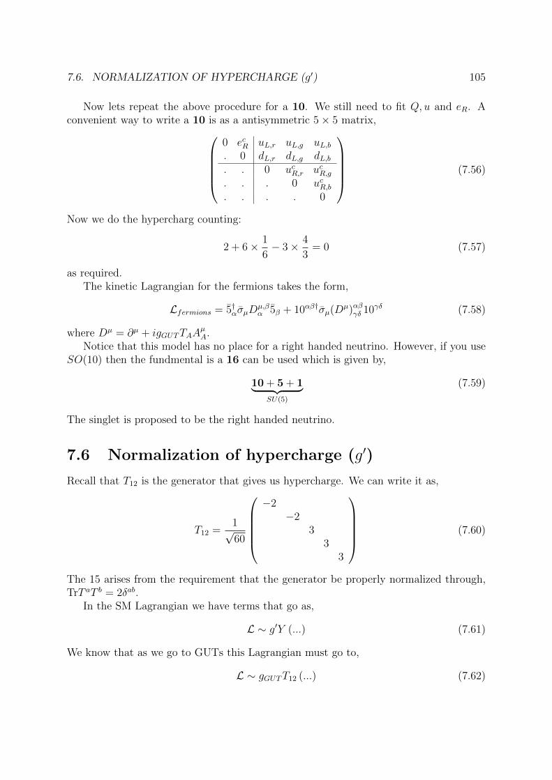
7.6. NORMALIZATION OF HYPERCHARGE (g′) 105
Now lets repeat the above procedure for a 10. We still need to fit Q, u and eR. Aconvenient way to write a 10 is as a antisymmetric 5× 5 matrix,
0 ecR uL,r uL,g uL,b. 0 dL,r dL,g dL,b. . 0 ucR,r ucR,g. . . 0 ucR,b. . . . 0
(7.56)
Now we do the hypercharg counting:
2 + 6× 1
6− 3× 4
3= 0 (7.57)
as required.The kinetic Lagrangian for the fermions takes the form,
Lfermions = 5†ασµDµ,βα 5β + 10αβ†σµ(Dµ)αβγδ 10γδ (7.58)
where Dµ = ∂µ + igGUTTAAµA.
Notice that this model has no place for a right handed neutrino. However, if you useSO(10) then the fundmental is a 16 can be used which is given by,
10 + 5 + 1︸ ︷︷ ︸SU(5)
(7.59)
The singlet is proposed to be the right handed neutrino.
7.6 Normalization of hypercharge (g′)
Recall that T12 is the generator that gives us hypercharge. We can write it as,
T12 =1√60
−2
−23
33
(7.60)
The 15 arises from the requirement that the generator be properly normalized through,TrT aT b = 2δab.
In the SM Lagrangian we have terms that go as,
L ∼ g′Y (...) (7.61)
We know that as we go to GUTs this Lagrangian must go to,
L ∼ gGUTT12 (...) (7.62)
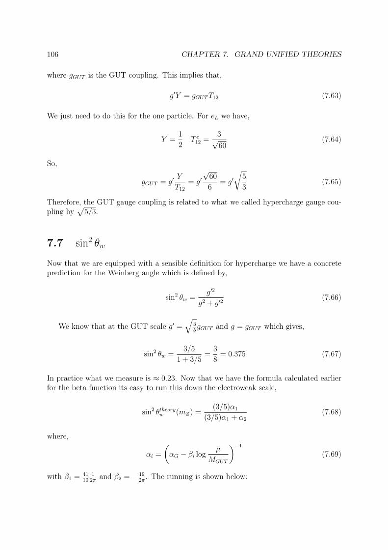
106 CHAPTER 7. GRAND UNIFIED THEORIES
where gGUT is the GUT coupling. This implies that,
g′Y = gGUTT12 (7.63)
We just need to do this for the one particle. For eL we have,
Y =1
2T e12 =
3√60
(7.64)
So,
gGUT = g′Y
T12
= g′√
60
6= g′
√5
3(7.65)
Therefore, the GUT gauge coupling is related to what we called hypercharge gauge cou-pling by
√5/3.
7.7 sin2 θw
Now that we are equipped with a sensible definition for hypercharge we have a concreteprediction for the Weinberg angle which is defined by,
sin2 θw =g′2
g2 + g′2(7.66)
We know that at the GUT scale g′ =√
35gGUT and g = gGUT which gives,
sin2 θw =3/5
1 + 3/5=
3
8= 0.375 (7.67)
In practice what we measure is ≈ 0.23. Now that we have the formula calculated earlierfor the beta function its easy to run this down the electroweak scale,
sin2 θtheoryw (mZ) =(3/5)α1
(3/5)α1 + α2
(7.68)
where,
αi =
(αG − βi log
µ
MGUT
)−1
(7.69)
with β1 = 4110
12π
and β2 = − 192π
. The running is shown below:
7.8. CHARGE QUANTIZATION 107
100 104 106 108 1010 1012 1014
0.25
0.30
0.35
Energy scale [GeV]
sin2θwtheory
We find,
sin2 θ(m2Z) ≈ 0.21 (7.70)
This is close to the true value but not exactly equal to. If you use supersymmetry theprediction becomes 0.23 as expected.
7.8 Charge Quantization
Charge in the SM is given by,
Q = T3 + Y (7.71)
Changing the coupling g′ effectively changes the hypercharge giving,
Q = T3 +
√5
3T12 (7.72)
The fundamental has the charges,
5→
000
1/2−1/2
+
1/31/31/3−1/2−1/2
=
1/31/31/30−1
(7.73)
As promised electric charge is necessarily quantized. In particular, the charge of theelectron is a multiple of the charge of the downtype quarks as expected. Similarly theright handed lepton has a charge which is a multiple of the left handed quark doublet.
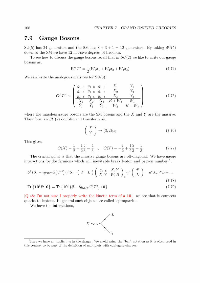
108 CHAPTER 7. GRAND UNIFIED THEORIES
7.9 Gauge Bosons
SU(5) has 24 generators and the SM has 8 + 3 + 1 = 12 generators. By taking SU(5)down to the SM we have 12 massive degrees of freedom.
To see how to discuss the gauge bosons recall that in SU(2) we like to write our gaugebosons as,
W aT a =1
2(W1σ1 +W2σ2 +W3σ3) (7.74)
We can write the analogous matrices for SU(5):
GATA ∼
g1−8 g1−8 g1−8 X1 Y1
g1−8 g1−8 g1−8 X2 Y2
g1−8 g1−8 g1−8 X3 Y3
X1 X2 X3 B +W3 W1
Y1 Y2 Y3 W2 B −W3
(7.75)
where the massless gauge bosons are the SM bosons and the X and Y are the massive.They form an SU(2) doublet and transform as,(
XY
)→ (3, 2)5/3 (7.76)
This gives,
Q(X) =1
2+
1
2
5
3=
4
3, Q(Y ) = −1
2+
1
2
5
3=
1
3(7.77)
The crucial point is that the massive gauge bosons are off-diagonal. We have gaugeinteractions for the fermions which will inevitable break lepton and baryon number 5,
5†(∂µ − igGUTGA
µTA)γµ5 =
(dc L
)( g1−8 X, YX, Y W,B
)µ
γµ(dc
L
)= dcXµγ
µL+ ...
(7.78)
Tr10† /D10
= Tr
10†
(/∂ − igGUTGa
µTa)
10
(7.79)
[Q 48: I’m not sure I properly write the kinetic term of a 10.] we see that it connectsquarks to leptons. In general such objects are called leptoquarks.
We have the interactions,
X
L
q
5Here we have an implicit γ0 in the dagger. We avoid using the “bar” notation as it is often used inthis context to be part of the definition of multiplets with conjugate charges.
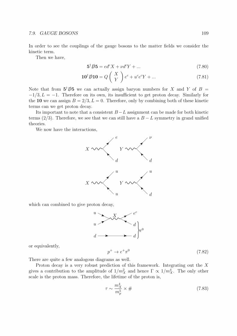
7.9. GAUGE BOSONS 109
In order to see the couplings of the gauge bosons to the matter fields we consider thekinetic term.
Then we have,
5† /D5 = edcX + νdcY + ... (7.80)
10† /D10 = Q
(XY
)ec + ucecY + ... (7.81)
Note that from 5† /D5 we can actually assign baryon numbers for X and Y of B =−1/3, L = −1. Therefore on its own, its insufficient to get proton decay. Similarly forthe 10 we can assign B = 2/3, L = 0. Therefore, only by combining both of these kineticterms can we get proton decay.
Its important to note that a consistent B−L assignment can be made for both kineticterms (2/3). Therefore, we see that we can still have a B−L symmetry in grand unifiedtheories.
We now have the interactions,
X
e
d
Y
ν
d
X
u
u
Y
u
d
which can combined to give proton decay,
d d
u
uX
ec
dπ0
or equivalently,p+ → e+π0 (7.82)
There are quite a few analogous diagrams as well.Proton decay is a very robust prediction of this framework. Integrating out the X
gives a contribution to the amplitude of 1/m2X and hence Γ ∝ 1/m4
X . The only otherscale is the proton mass. Therefore, the lifetime of the proton is,
τ ∼ m4X
m5p
×# (7.83)
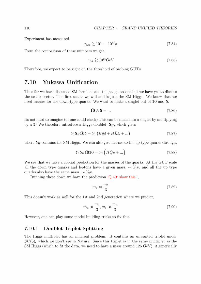
110 CHAPTER 7. GRAND UNIFIED THEORIES
Experiment has measured,τexp & 1031 − 1033y (7.84)
From the comparison of these numbers we get,
mX & 1015GeV (7.85)
Therefore, we expect to be right on the threshold of probing GUTs.
7.10 Yukawa Unification
Thus far we have discussed SM fermions and the gauge bosons but we have yet to discussthe scalar sector. The first scalar we will add is just the SM Higgs. We know that weneed masses for the down-type quarks. We want to make a singlet out of 10 and 5.
10⊗ 5 = ... (7.86)
Its not hard to imagine (or one could check) This can be made into a singlet by multiplyingby a 5. We therefore introduce a Higgs doublet, 5H , which gives
Y15H 105 = Y1
(Hqd+HLE + ...
)(7.87)
where 5H contains the SM Higgs. We can also give masses to the up-type quarks through,
Y25H 1010 = Y2
(HQu+ ...
)(7.88)
We see that we have a crucial prediction for the masses of the quarks. At the GUT scaleall the down type quarks and leptons have a given mass, ∼ Y1v, and all the up typequarks also have the same mass, ∼ Y2v.
Running these down we have the prediction [Q 49: show this.],
mτ ≈mb
3(7.89)
This doesn’t work as well for the 1st and 2nd generation where we predict,
mµ ≈ms
3,me ≈
md
3(7.90)
However, one can play some model building tricks to fix this.
7.10.1 Doublet-Triplet Splitting
The Higgs multiplet has an inherent problem. It contains an unwanted triplet underSU(3)c which we don’t see in Nature. Since this triplet is in the same multiplet as theSM Higgs (which to fit the data, we need to have a mass around 126 GeV), it generically
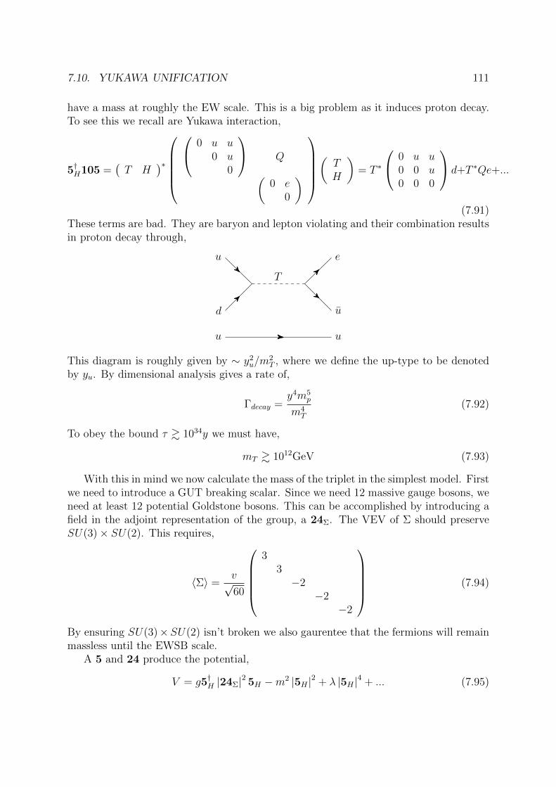
7.10. YUKAWA UNIFICATION 111
have a mass at roughly the EW scale. This is a big problem as it induces proton decay.To see this we recall are Yukawa interaction,
5†H105 =(T H
)∗ 0 u u
0 u0
Q(0 e
0
)(TH
)= T ∗
0 u u0 0 u0 0 0
d+T ∗Qe+...
(7.91)These terms are bad. They are baryon and lepton violating and their combination resultsin proton decay through,
d
u
T
e
u
u u
This diagram is roughly given by ∼ y2u/m
2T , where we define the up-type to be denoted
by yu. By dimensional analysis gives a rate of,
Γdecay =y4m5
p
m4T
(7.92)
To obey the bound τ & 1034y we must have,
mT & 1012GeV (7.93)
With this in mind we now calculate the mass of the triplet in the simplest model. Firstwe need to introduce a GUT breaking scalar. Since we need 12 massive gauge bosons, weneed at least 12 potential Goldstone bosons. This can be accomplished by introducing afield in the adjoint representation of the group, a 24Σ. The VEV of Σ should preserveSU(3)× SU(2). This requires,
〈Σ〉 =v√60
3
3−2
−2−2
(7.94)
By ensuring SU(3)×SU(2) isn’t broken we also gaurentee that the fermions will remainmassless until the EWSB scale.
A 5 and 24 produce the potential,
V = g5†H |24Σ|2 5H −m2 |5H |2 + λ |5H |4 + ... (7.95)
112 CHAPTER 7. GRAND UNIFIED THEORIES
The 5H is made up of the SM doublet and a new color triplet Higgs,
5H =
(TH
)(7.96)
where H = (1, 2)1, T = (3, 1)−1/3. The masses of the Higgses are,
m2H ∼ 32 〈Σ〉2 +m2 (7.97)
m2T ∼ 22 〈Σ〉2 +m2 (7.98)
To have mT at around the GUT scale we need 〈Σ〉 to be around the GUT scale. Therefore,the only way to have a light Higgs is to get 〈Σ〉2 and m2 to cancel to very high precision.This is called the doublet triplet splitting problem. For SUSY this problem turns out tobe much more severe.
7.11 SO(10)
One might wonder why we bothered to put the matter fields into different representations.The number of matter fields in the SM for each generation is,
quark︷ ︸︸ ︷3× 4 + 3︸︷︷︸
lepton
= 15 (7.99)
We could have put all the SM fields of one generation into a 15. While this is appealing,it can be very problematic when trying to build a Higgs sector for this theory as it willinevitably give the same Yukawa for all the matter fields, including the neutrinos. Neu-trinos will form extremely massive Majorana spinors, which horribly contradicts reality.Furthermore, we can’t just use the seesaw mechanism since there are no right handedneutrinos (keep in mind that adding a field here necessarily means a whole new mutlipletwith a new set of particles that we don’t observe.
While this idea of putting all the fields in the same multiplet is a big nuisance inSU(5), its completely natural in SO(10). SO(10) has the subgroups,
SU(5)× U(1) (7.100)
SU(4)× SU(2)× SU(2) (7.101)
[Q 50: Why do I get SU(4)× SU(2) using Dynkin diagrams?]The possibility of breaking through SU(5)×U(1) is intriguing as all the good features
we mentioned earlier will still hold here. The only difference is that we have an extraU(1) symmetry. This U(1) can be identified with B−L. Since we don’t see an additionalmassless gauge boson in Nature, this symmetry must be broken. However, the scale ofthis breaking can be anything.
All the SM can fit neatly into 16, where now we have room for an additional field,the right handed neutrino. A yukawa interaction will need to involve two 16’s. To find
7.11. SO(10) 113
the possible Higgs representations we need to know the possible charges of a product ofmatter fields,
16× 16 = 10 + 126 + 120 (7.102)
Therefore, the simplest possibility is to have a Higgs of 10 and use a two Higgs doubletmodel,
10 = 5 + 5 (7.103)
The terms in the Lagrangian in terms of the SU(5) reps are
L = 161610H = 5105H + 10× 105H + 155H (7.104)
where 1 is the right handed neutrino. We see that the SM particles get masses,
mu = mν = −λvu md = me = −λvd (7.105)
However, there can be an additional mass for the right handed neutrino arising from theGUT breaking Higgs. Suppose the GUT breaking scalar is a ¯126 (with a scalar φ) suchthat it has a Yukawa with the right handed neutrinos.
λN νcRνLφ (7.106)
This won’t break the SM gauge symmetry if it has U(1) = 10 and B − L = −2. Whenthe scalar gets a VEV it will break B − L but since B − L is even it will leave matterparity,
Rm = (−1)3(B−L) (7.107)
invariant. Matter parity is equivalent to the much more well known R parity,
Rp = (−1)3(B−L)+2s (7.108)
Therefore, GUTs actually provide a natural motivation forRp which is commonly imposedad hoc in the MSSM.
Furthermore, we now have the neutrino mass matrix,(0 λvuλvu 〈φ〉
)(7.109)
To get neutrino masses at around the eV scale we need 〈φ〉 ∼ 1013GeV, which is con-veniently very close to the GUT scale. This was the original motivation for the famoussee-saw mechanism.
An alternative to the breaking pattern discussed above is to use the Pati Salammodels. Recall that Pati Salam theories are made using SU(4)c. SU(4)c is homomorphicto SO(6).6 Furthermore, the other two groups in Pati Salam are given by SU(2)×SU(2)which is homomorphic to SO(4). Therefore, Pati Salam is equivalent to,
SO(6)× SO(4) (7.110)
6Recall that a group homomorphism is a mapping f : G → H such that for every element of g:f(g1 · g2) = f(g1) · f(g2). In contract an group isomorphism is a mapping that can go both from G→ Hand from H → G.
114 CHAPTER 7. GRAND UNIFIED THEORIES
Its easy to show (or guess) that this is a subgroup of SO(10). The spinor representation ofSO(10) contains one family of quarks and leptons. In fact if you take SO(10) and breakit up into Pati salam you get (recall that the notation here is (SU(4)c, SU(2)L, SU(2)R)),
16→ (4, 2, 1) + (4, 1, 2) (7.111)
For the Higgses we have through SSB,
10→ (6, 1, 1) + (1, 2, 2) (7.112)
7.12 Orbifold GUTs
Current four dimensional solutions of the doublet-triplet splitting problem aren’t pretty.They either require very large representations for the scalar sector or significant fine-tuning as shown above. Its hard to imagine these theories coming out of theory ofquantum gravity such as string theory. The mainstream solution to this problem is toconsider orbifold GUTs. The idea that the GUT is a GUT in 5 or 6 dimensions but whenwe go to 4 dimensions you have broken the unification symmetry down the SM.
Consider a SO(3) gauge theory which is defined on a circle (by this we mean that thefields have periodic boundary conditions in the fifth dimension) ,
Minkowski︷︸︸︷M4 ⊗S1 (7.113)
The gauge bosons are given by,
AM(xµ, y) ≡ AaM(xµ, y)T a (7.114)
where M = 0, 1, 2, 3, 5 and y goes from 0 to 2πR. The field strength tensor is given by,
FMN(x, y) = F aMNT
a = ∂MAN − ∂NAM + i [AM , AN ] (7.115)
The Lagrangian is given by,
L5 = − 1
2g25k
TrFMNFMN (7.116)
where k is the normalization of the generators,
TrT aT b = kδab (7.117)
The gauge bosons transform under gauge transformations as,
AM(xµ, y)→ UAMU† − iU∂MU † (7.118)
where U = exp (iθa(xµ, y)T a).
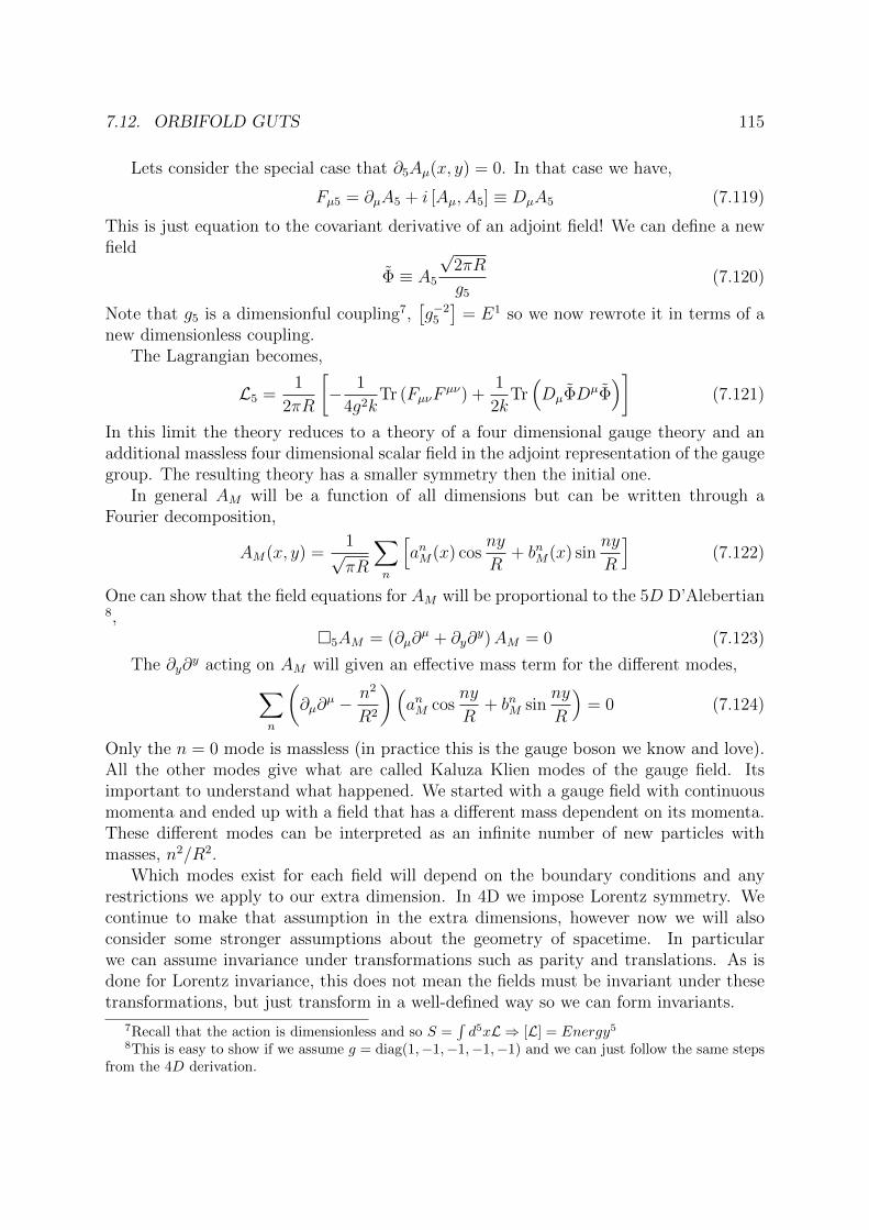
7.12. ORBIFOLD GUTS 115
Lets consider the special case that ∂5Aµ(x, y) = 0. In that case we have,
Fµ5 = ∂µA5 + i [Aµ, A5] ≡ DµA5 (7.119)
This is just equation to the covariant derivative of an adjoint field! We can define a newfield
Φ ≡ A5
√2πR
g5
(7.120)
Note that g5 is a dimensionful coupling7,[g−2
5
]= E1 so we now rewrote it in terms of a
new dimensionless coupling.The Lagrangian becomes,
L5 =1
2πR
[− 1
4g2kTr (FµνF
µν) +1
2kTr(DµΦDµΦ
)](7.121)
In this limit the theory reduces to a theory of a four dimensional gauge theory and anadditional massless four dimensional scalar field in the adjoint representation of the gaugegroup. The resulting theory has a smaller symmetry then the initial one.
In general AM will be a function of all dimensions but can be written through aFourier decomposition,
AM(x, y) =1√πR
∑n
[anM(x) cos
ny
R+ bnM(x) sin
ny
R
](7.122)
One can show that the field equations for AM will be proportional to the 5D D’Alebertian8,
5AM = (∂µ∂µ + ∂y∂
y)AM = 0 (7.123)
The ∂y∂y acting on AM will given an effective mass term for the different modes,∑
n
(∂µ∂
µ − n2
R2
)(anM cos
ny
R+ bnM sin
ny
R
)= 0 (7.124)
Only the n = 0 mode is massless (in practice this is the gauge boson we know and love).All the other modes give what are called Kaluza Klien modes of the gauge field. Itsimportant to understand what happened. We started with a gauge field with continuousmomenta and ended up with a field that has a different mass dependent on its momenta.These different modes can be interpreted as an infinite number of new particles withmasses, n2/R2.
Which modes exist for each field will depend on the boundary conditions and anyrestrictions we apply to our extra dimension. In 4D we impose Lorentz symmetry. Wecontinue to make that assumption in the extra dimensions, however now we will alsoconsider some stronger assumptions about the geometry of spacetime. In particularwe can assume invariance under transformations such as parity and translations. As isdone for Lorentz invariance, this does not mean the fields must be invariant under thesetransformations, but just transform in a well-defined way so we can form invariants.
7Recall that the action is dimensionless and so S =∫d5xL ⇒ [L] = Energy5
8This is easy to show if we assume g = diag(1,−1,−1,−1,−1) and we can just follow the same stepsfrom the 4D derivation.
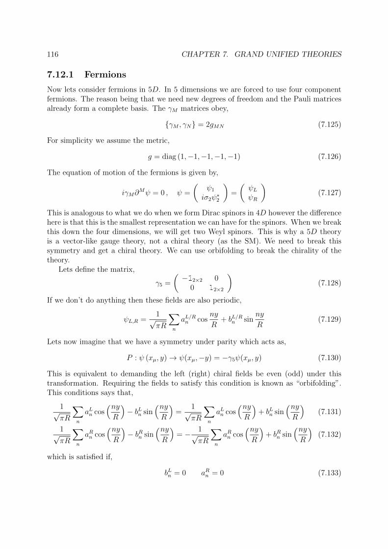
116 CHAPTER 7. GRAND UNIFIED THEORIES
7.12.1 Fermions
Now lets consider fermions in 5D. In 5 dimensions we are forced to use four componentfermions. The reason being that we need new degrees of freedom and the Pauli matricesalready form a complete basis. The γM matrices obey,
γM , γN = 2gMN (7.125)
For simplicity we assume the metric,
g = diag (1,−1,−1,−1,−1) (7.126)
The equation of motion of the fermions is given by,
iγM∂Mψ = 0 , ψ =
(ψ1
iσ2ψ∗2
)=
(ψLψR
)(7.127)
This is analogous to what we do when we form Dirac spinors in 4D however the differencehere is that this is the smallest representation we can have for the spinors. When we breakthis down the four dimensions, we will get two Weyl spinors. This is why a 5D theoryis a vector-like gauge theory, not a chiral theory (as the SM). We need to break thissymmetry and get a chiral theory. We can use orbifolding to break the chirality of thetheory.
Lets define the matrix,
γ5 =
(−12×2 0
0 12×2
)(7.128)
If we don’t do anything then these fields are also periodic,
ψL,R =1√πR
∑n
aL/Rn cosny
R+ bL/Rn sin
ny
R(7.129)
Lets now imagine that we have a symmetry under parity which acts as,
P : ψ (xµ, y)→ ψ(xµ,−y) = −γ5ψ(xµ, y) (7.130)
This is equivalent to demanding the left (right) chiral fields be even (odd) under thistransformation. Requiring the fields to satisfy this condition is known as “orbifolding”.This conditions says that,
1√πR
∑n
aLn cos(nyR
)− bLn sin
(nyR
)=
1√πR
∑n
aLn cos(nyR
)+ bLn sin
(nyR
)(7.131)
1√πR
∑n
aRn cos(nyR
)− bRn sin
(nyR
)= − 1√
πR
∑n
aRn cos(nyR
)+ bRn sin
(nyR
)(7.132)
which is satisfied if,
bLn = 0 aRn = 0 (7.133)
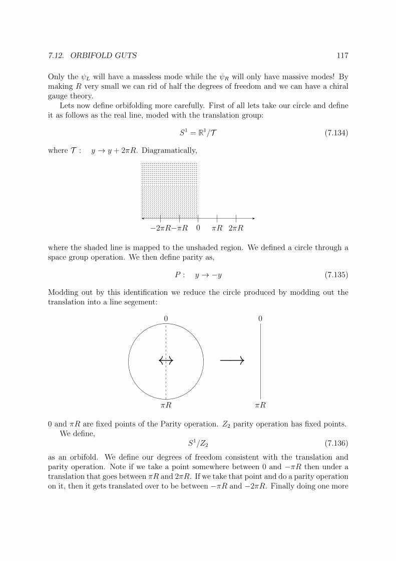
7.12. ORBIFOLD GUTS 117
Only the ψL will have a massless mode while the ψR will only have massive modes! Bymaking R very small we can rid of half the degrees of freedom and we can have a chiralgauge theory.
Lets now define orbifolding more carefully. First of all lets take our circle and defineit as follows as the real line, moded with the translation group:
S1 = R1/T (7.134)
where T : y → y + 2πR. Diagramatically,
−2πR−πR 0 πR 2πR
where the shaded line is mapped to the unshaded region. We defined a circle through aspace group operation. We then define parity as,
P : y → −y (7.135)
Modding out by this identification we reduce the circle produced by modding out thetranslation into a line segement:
↔
0
πR
−→
πR
0
0 and πR are fixed points of the Parity operation. Z2 parity operation has fixed points.We define,
S1/Z2 (7.136)
as an orbifold. We define our degrees of freedom consistent with the translation andparity operation. Note if we take a point somewhere between 0 and −πR then under atranslation that goes between πR and 2πR. If we take that point and do a parity operationon it, then it gets translated over to be between −πR and −2πR. Finally doing one more
118 CHAPTER 7. GRAND UNIFIED THEORIES
translation we get between 0 and πR. The next effect of this combination, T PT isequivalent to the Parity operation, i.e.,
T PT = P (7.137)
Now lets represent this parity operation on fields. For the time being lets think of Φto being in some representation of SO(3). Parity takes the form:
P : Φ(x, y)→ Φ(x,−y) = PΦ(x, y) (7.138)
(P here represents a phase) where, P2 = 1 implies that P 2 = 1 and P = ±1.The situation is similar for translations. Typically we start with periodic functions.
But since this is a gauge theory we have periodic functions that come back to the samefunction up to a finite gauge transformation,
T : Φ(x, y)→ Φ(x, y + 2πR) = TΦ(x, y) (7.139)
The finite gauge transformation can quite generally be written in the form,
T = exp
(i
∮〈A5〉 dy
)(7.140)
This is known as a Wilson line. Instead of the functions being purely periodic they areperiodic up to the possibility of a phase. T is an element of the SO(3) group and hencewe also have T 2 = 1.
Due to T PT = P we also have 9,
(PT )2 = 1 ⇒ (PT )2 = 1 (7.141)
where we can define,
P ′ ≡ PT (7.142)
We can now think of imposing the group,
S1/Z2 = S1/Z2 ⊗ Z ′2 (7.143)
We now take our fields and assume they obey,
P : Φ(y)→ Φ(−y) = PΦ(y) (7.144)
P ′ Φ(y)→ Φ(−y + 2πR) = P ′Φ(y) (7.145)
We can either do a parity operation around point zero or around a point πR. We haveparity eigenstate possibilities,
(P, P ′) = (±,±) (7.146)
9Here we assume that you can simultaneously diagonalize P and T .
7.12. ORBIFOLD GUTS 119
Our components (i.e., the Fourier decomposition modes) will differ depending on thesechoices,
ξm(+,+)(y) ≈ cosmy
R(7.147)
ξm(+,−)(y) ≈ cos
[(m+
1
2
)y/R
](7.148)
ξm(−,+)(y) ≈ sin
[(m+
1
2
)y/R
](7.149)
ξm(−,−)(y) ≈ sin [(m+ 1)y/R] (7.150)
To understand why this is take for example the (+,−) mode. It should be even under Pand odd under P ′. We have,
ξm(+,−)P−→ cos
[−(m+
1
2
)y/R
]= ξm(+,−) (7.151)
ξm(+,−)P ′−→ cos
[−(m+
1
2
)y/R + 2π
(m+
1
2
)]= ξm(+,−) = −ξm(+,−) (7.152)
as required. Note that any function which is positive under the boundary conditions, thewavefunction in the fifth direction does not vanish on that boundary. So e.g. at the zeroboundary, ξm(+,±) has nonzero wavefunction.
We see that the 0 boundary and the πR boundary are totally different. We will thinkof them soon when we consider the SO(3) gauge theory as different branes with differentboundary conditions.[Q 51: Define branes carefully.]
Further, note the Kaluza Klien masses for the states are,
M2KK =
+ + m2/R2
+−(m+ 1
2
)/R2
−+(m+ 1
2
)/R2
−− (m+ 1)2 /R2
(7.153)
Therefore, only the ++ boundary condition has massless modes. We will now considerhow we can use these boundary conditions to break the gauge symmetry.
As an example lets consider SO(3) gauge theory. We will take the Wilson line, T , tobe given by,
T = exp(iπT 3
)=
−1−1
1
(7.154)
where T 3 is the generator in the adjoint representation. This is equivalent to saying thatonly the third component of the generator receives a vacuum expectation value. Doingthe integral from 0 to 2πR we are assuming,
〈A5〉 =1
2R(7.155)
120 CHAPTER 7. GRAND UNIFIED THEORIES
[Q 52: Clarify this.] Lets choose certain parities of the fields.The Aaµ fields appear in the field strength,
Fµν = ∂µAν − ∂νAµ − i [Aµ, Aν ] (7.156)
We need parity to be a symmetry of the theory. Fµν can only be a parity eigenstate onlyif
AaµP−→ Aaµ (7.157)
A5 appears in the field strength,
Fµ5 = ∂µA5 − ∂5Aµ − i [Aµ, A5] (7.158)
Under the parity operator ∂5 changes sign and Aaµ does not which implies that ∂µA5 has
to change sign as well. This can only be the case if A5P−→ −A5.
Under the second parity operation we have (remember that T is real and Aµ are inthe adjoint representation),
A′µ = TPAµPT (7.159)
For A3µ which transforms as,
A3′µ = TPA3
µT3PT (7.160)
the transformation is simple since A3µ is P invariant and trivially T invariant as well.
For A35 we still have,
TT 3T = T 3 (7.161)
but its also odd under P . This results in A35 also being odd under P ′.
To consider the off diagonal component we define the quantities,
W±µ =
1√2
(A1µ ∓ iA2
µ
)T± = T1 ± iT2 (7.162)
then,TT±T = ±T± (7.163)
One can show that,
W±µ = (+,−) (7.164)
W±5 = (−,+) (7.165)
[Q 53: check.]We have broken up the theory so the different gauge bosons have different parities.
The only gauge boson that has a massless mode is A3µ. Therefore, we’ve broken down
SO(3) down to SO(2) ≈ U(1). The lightest gauge boson has mass(m+ 1
2
)/R.
Lastly we note that an infinitesimal gauge transformations for the fields must beconsistent with the boundary conditions. For example A3
µ has ++ boundary conditionsand so under a gauge transformation is,
δA3µ = ∂µθ
3++ (7.166)
7.12. ORBIFOLD GUTS 121
Similarly,δA1/2
µ = ∂µθ1/2+− (7.167)
The A1/2µ fields vanish at the πR fixed point. We say that in bulk we have an SO(3)
gauge theory. We call the y = 0 brane an SO(3) brane since there all gauge fieldstransform in the same way. [Q 54: Aren’t the off-diagonal gauge fields still massive?] Weonly have SO(2) symmetry on the right brane.
0 πR
SO(3) SO(2)
7.12.2 SU(5) SUSY Orbifold GUTs
We consider an orbifolding,M4 ⊗ S1/Z2 ⊗ Z ′2 (7.168)
We now think of an N = 1 supersymmetry is 5D. The gauge sector of superfield infive dimensions contains,
V5 = AM , λ, λ′, σ (7.169)
where λ and λ′ are two Weyl spinors and σ is a scalar where all fields are in the adjointrepresentation of SU(5). This can be thought of as N = 2 supersymmetry in 4D. Thegauge multiplet in 4D is,
V = Aµ, λ (7.170)
and a chiral field,
Σ =
σ + A5√
2, λ′
(7.171)
So out of the 5D adjoint multiplet we get a 4D N = 1 gauge multiplet and a 4D N = 1chiral multiplet. these two together form a N = 2 representation. These will go in thebulk. We will also put our higgses in the bulk. The Higgs make up two multiplets:
H = H5, Hc5 (7.172)
Together these form an N = 1 5D multiplet. We also introduce,
H =H5, H
c5
(7.173)
These also go in the bulk. Pictorally we will have,
0 πR
SU(5)
(V,Σ)
(H, H)
SU(5) brane SM brane
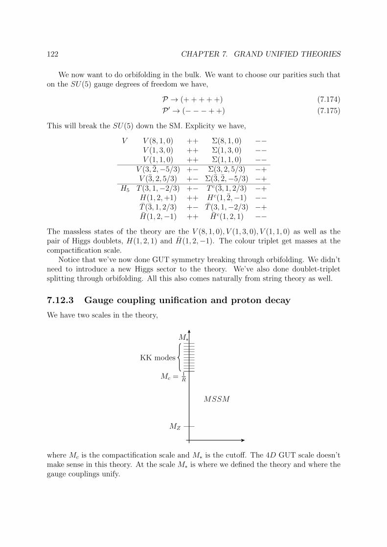
122 CHAPTER 7. GRAND UNIFIED THEORIES
We now want to do orbifolding in the bulk. We want to choose our parities such thaton the SU(5) gauge degrees of freedom we have,
P → (+ + + + +) (7.174)
P ′ → (−−−+ +) (7.175)
This will break the SU(5) down the SM. Explicity we have,
V V (8, 1, 0) ++ Σ(8, 1, 0) −−V (1, 3, 0) ++ Σ(1, 3, 0) −−V (1, 1, 0) ++ Σ(1, 1, 0) −−
V (3, 2,−5/3) +− Σ(3, 2, 5/3) −+V (3, 2, 5/3) +− Σ(3, 2,−5/3) −+
H5 T (3, 1,−2/3) +− T c(3, 1, 2/3) −+H(1, 2,+1) ++ Hc(1, 2,−1) −−T (3, 1, 2/3) +− T (3, 1,−2/3) −+H(1, 2,−1) ++ Hc(1, 2, 1) −−
The massless states of the theory are the V (8, 1, 0), V (1, 3, 0), V (1, 1, 0) as well as thepair of Higgs doublets, H(1, 2, 1) and H(1, 2,−1). The colour triplet get masses at thecompactification scale.
Notice that we’ve now done GUT symmetry breaking through orbifolding. We didn’tneed to introduce a new Higgs sector to the theory. We’ve also done doublet-tripletsplitting through orbifolding. All this also comes naturally from string theory as well.
7.12.3 Gauge coupling unification and proton decay
We have two scales in the theory,
MZ
Mc = 1R
M∗
KK modes
MSSM
where Mc is the compactification scale and M∗ is the cutoff. The 4D GUT scale doesn’tmake sense in this theory. At the scale M∗ is where we defined the theory and where thegauge couplings unify.

Bibliography
123