algebraic number theory ben green

Algebraic Number Theory

Ben Green

Contents

Preface 1

0.1. A brief introduction 1

0.2. These notes 2

0.3. Prerequisites 2

Chapter 1. Algebraic numbers 3

1.1. Algebraic numbers. Minimal polynomials. 3

1.2. The algebraic numbers are a field 5

1.3. Number fields. The primitive element theorem 6

1.4. More examples 7

1.5. Conjugates and embeddings 8

1.6. Norms 10

1.7. Norms and determinants 12

1.8. Discriminants 14

Chapter 2. Algebraic integers 17

2.1. Algebraic integers 17

2.2. The ring of integers of a number field 19

2.3. Units 19

2.4. Integral bases 20

2.5. Quadratic fields 22

2.6. Computing an integral basis 23

Chapter 3. Irreducibles and factorisation 27

3.1. Basic concepts 27

3.2. Failure in Q[√−5] 28

3.3. The usefulness of unique factorisation 29

Chapter 4. Ideals and their basic properties 31

4.1. Ideals and principal ideals 31

4.2. A nonprincipal ideal 32

4.3. Basic properties of ideals 33

4.4. Norms. Integral basis for an ideal. 33

v

vi CONTENTS

4.5. Multiplying ideals. Prime ideals. 34

Chapter 5. Unique factorisation into prime ideals 37

5.1. Prime factors 37

5.2. Finding an inverse 38

5.3. Cancellation, divisibility and prime ideals 40

5.4. Proof of unique factorsation 41

5.5. Finding the prime ideals 41

Chapter 6. Irreducibles and factorisation, revisited 43

6.1. Irreducibles and primes 43

6.2. UFDs and PIDs 44

Chapter 7. More on norms of ideals 45

7.1. Norm of a product 45

7.2. Ideals divide their norms 46

7.3. Automorphisms 47

Chapter 8. Q(√−5) revisited 49

Chapter 9. Factoring into prime ideals in practice 51

9.1. Splitting of rational primes 51

9.2. Irreducibility over Z and mod p 52

9.3. Dedekind’s lemma 53

9.4. Example: Splitting of primes in Q(i) 54

9.5. Factoring a general ideal 54

Chapter 10. The class group 57

10.1. Basic definitions 57

10.2. Minkowski bound. Finiteness of the class group. 58

10.3. Elements with small norm 59

10.4. Geometry of numbers 60

10.5. Elements with small norm: imaginary quadratic fields 60

10.6. Elements with small norm: general case 61

Chapter 11. Example class group calculations 65

11.1. Q(i) and sums of squares 65

11.2. Q(√−5) 66

11.3. Q(√−29) 66

11.4. Q(√−163) and the Rabinowitch Phenomenon 68

Chapter 12. An elliptic curve 71

CONTENTS vii

Chapter 13. The case n = 3 of Fermat’s last theorem 73

Chapter 14. Quadratic forms and the class group 77

14.1. From ideal classes to Γ \H. 77

14.2. Quadratic forms from points of H 79

14.3. Action of SL2(Z) and reduction theory 80

14.4. Integral binary quadratic forms and Heegner points 82

14.5. Example: Q(√−29) 83

14.6. Further remarks 84

Chapter 15. Unsolved problems 85

Appendix A. Free abelian groups and lattices 87

Appendix B. Geometry of numbers 89

Appendix C. Gauss’s Lemma 91

Appendix D. Vandermonde determinants 93

Preface

0.1. A brief introduction

Every positive integer greater than one may be factored into primes, and this

factorisation is unique up to the ordering of the primes. You have known this fact

since school (though the first time you saw a proof may well have been last year,

in Part A). It is impossible to imagine doing number theory without it.

Does unique factorisation into primes generalise? To understand why one might

care about this question, let us look at some theorems about diophantine equations

(equations to be solved in integers) that have been proven by mathematicians in

the past.

• considered by Fermat and Euler: the only solutions to y2 + 2 = x3 are

x = 3, y = ±5.

• Fermat: if p is a prime, p = x2 + y2 has a solution if and only if p ≡1(mod 4).

• Euler: if x3 + y3 = z3, one of x, y, z is zero (the case n = 3 of Fermat’s

last theorem).

• Nagell (conjecture of Ramanujan): if x2 + 7 = 2n, then n = 3, 4, 5, 7, 15.

A common feature of these equations is that they admit natural factorisations,

but not over the integers. Respectively, they may be factored as

(y +√−2)(y −

√−2) = x3,

p = (x+ iy)(x− iy),

(x+ y)(x+ ζy)(x+ ζ2y) = z3

(where ζ = e2πi/3) and

(x+√−7)(x−

√−7) = 2n.

To proceed further, one needs to understand the more general “number systems” in

which we have written these factorisations. This – especially the question of unique

factorisation into primes – is the main theme of the course.

1

2 PREFACE

0.2. These notes

These are notes I wrote to teach the course B3.4 Algebraic Number Theory at

Oxford in Hilary Term 2020. They cover the examinable material of that course as

well as some extra material on the link between class groups of imaginary quadratic

fields and binary quadratic forms. I was able to cover the material fairly comfortably

in sixteen 55-minute lectures, omitting only the proof of the Minkowski bound in

the general case.

In making these notes available to a general audience, I have omitted any men-

tion of which topics and proofs are considered examinable in the Oxford course.

In preparing the notes I used various books, particularly Stewart and Tall, as well

as previous notes by Victor Flynn, building on earlier notes of Neil Dummigan, Alan

Lauder and Roger Heath-Brown. In particular, most of the illustrative examples

are lifted directly from those notes.

Please send any corrections to

[email protected].

0.3. Prerequisites

Students taking B3.4 are expected to have attended the second year course Rings

and Modules, which covers the basic theory of rings and ideals, UFDs, PIDs and

so on. In the notes I recall a lot of this material, often with self-contained proofs.

A third year course on Galois theory is also listed as a prerequisite, but very little

Galois theory is actually used in this introductory course. The few sections requiring

Galois theory are starred.

I assume that students have taken a first course in number theory and cer-

tainly that they are familiar with modular arithmetic, as well as the statements of

quadratic reciprocity.

CHAPTER 1

Algebraic numbers

In this chapter we introduce the basic objects of the course.

1.1. Algebraic numbers. Minimal polynomials.

Definition 1.1.1. A complex number α is algebraic if it is the solution to some

polynomial equation with coefficients in Q. The set of all algebraic numbers is

denoted by Q.

Examples. Every rational is algebraic, as are i,√

2, 31/5 . . . but not e, π (though

we shall not prove this here!). Q is countable, since one may enumerate the poly-

nomials over Q, and each has only finitely many roots.

Lemma 1.1.2 (Minimal polynomial). Suppose that α ∈ Q. Then there is a

unique nonzero monic irreducible polynomial mα(X) satisfied by α, which we call

the minimal polynomial of α. If f ∈ Q[X] is any other polynomial satisfied by α

then mα|f .

Proof. Take mα to be a monic nonzero polynomial of least degree satisfied by α. If

mα were reducible, say mα(X) = f(X)g(X) with deg f, deg g < degmα, then since

mα(α) = 0 we have f(α)g(α) = 0, whence either f(α) = 0 or g(α) = 0, contrary to

the minimality of degmα.

Now let f ∈ Q[X] be some polynomial satisfied by α. By the Euclidean algo-

rithm we may write f(X) = mα(X)q(X) + r(X) with deg r < degmα. If f(α) = 0

then, since mα(α) = 0, we have r(α) = 0. By the minimality of deg(mα), we must

have r = 0, and so mα|f .

The uniqueness of mα follows immediately, since the only monic irreducible f

for which mα|f is mα itself.

Examples. The minimal polynomial mi(X) is X2 + 1. The minimal polynomial

m√2(X) is X2 − 2. If ω = e2πi/3 is a primitive third root of unity then mω(X) is

not X3 − 1, since this is a reducible polynomial; rather, mω(X) = X2 +X + 1.

Given any complex number α, write Q(α) for the smallest field containing Q and

α; this will consist of all fractions p(α)/q(α), where p, q ∈ Q[X] are polynomials.

3

4 1. ALGEBRAIC NUMBERS

Recall that if K,L are two fields with K ⊇ L then the degree [K : L] is the degree

of K, considered as a vector space over L (it may be infinite).

Lemma 1.1.3. Let α ∈ C. Then α is algebraic if, and only if, [Q(α) : Q] < ∞.

Suppose that α is algebraic. Then Q(α) = Q[α]. Suppose that mα, the minimal

polynomial for α, has degree n. Then a basis for Q(α) as a vector space over Q is

1, α, . . . , αn−1, that is to say Q(α) may be identified with the polynomials in α of

degree < n, and hence [Q(α) : Q] = degmα = n.

Proof. Suppose first that [Q(α) : Q] is finite, say equal to n. In particular, the

numbers 1, α, . . . , αn must be linearly dependent over Q, which means precisely

that α satisfies some polynomial equation with coefficients in Q (of degree 6 n)

and hence is algebraic.

In the other direction, suppose that α ∈ Q, and that mα is the minimal poly-

nomial of α, with degmα = n. Consider the evaluation map Q[X] → Q[α], which

sends f(X) to f(α). This is a surjective ring homomorphism whose kernel is the

set of polynomials in Q[X] satisfied by α. As we saw above, this is precisely (mα),

the ideal generated by mα. Therefore

Q[α] ∼= Q[X]/(mα).

Now (mα) is a maximal ideal in Q[X] (since all ideals in Q[X] are principal, and

if (mα) ⊆ (f) then f |mα and so (f) = (1) or (mα)). Therefore the quotient

Q[X]/(mα) is actually a field. We have shown that the polynomial ring Q[α] is in

fact a field, and so of course it must be Q(α).

Suppose that f(α) ∈ Q[α]. By the Euclidean algorithm, f(X) = mα(X)q(X) +

r(X) where deg r < n, and so f(α) = r(α). That is, Q[α] is spanned by 1, α, . . . , αn−1.

In the other direction, these elements are independent over Q since otherwise there

would be a nonzero polynomial of degree < n satisfied by α.

Remark. To help in understanding all this, let us explain a little more explicitly

and algorithmically why inverses exist in Q[α], a fact which is surprising at first

sight. Let f(α) ∈ Q[α], f(α) 6= 0. Then f is not divisible by mα and so is coprime

it. By the Euclidean algorithm there are polynomials q, p such that f(X)q(X) +

mα(X)p(X) = 1. Thus f(α)q(α) = 1, so q(α) is the inverse of f(α).

Examples. The field Q(i) = {a+ bi : a, b ∈ Q}, with the inverse being given by1

a+bi = a−bia2+b2 .

Similarly Q(√

2) = {a+ b√

2 : a, b ∈ Q}, with 1a+b√

2= a−b

√2

a2−2b2 .

Corollary 1.1.4. Suppose that α satisfies an equation of degree n over Q.

Then [Q(α) : Q] 6 n.

1.2. THE ALGEBRAIC NUMBERS ARE A FIELD 5

Proof. The minimal polynomial of α has degree 6 n, so the result follows straight

away from Lemma 1.1.3.

Arbitrary fields. Everything in this section in fact holds with Q replaced by

an arbitrary field k, and the proofs are essentially the same. The definitions of

algebraic and minimal polynomial must all be taken with respect to k. We did not

state results in this generality, for the following reasons:

• For almost the entire course, only the case k = Q is important;

• When k = Q, we can cheat somewhat, at least from the point of view

of exposition, because we already have the complex numbers C at our

disposal, in which we may locate Q as a specific subset. For general

fields k, extensions k(α) and an algebraic closure k must be constructed

abstractly. (This is probably the “correct” way to proceed when k = Qas well.)

In particular we have the following.

Lemma 1.1.5. Let k be a field. If α satisfies a polynomial of degree n over k,

then k[α] = k(α) is a field and [k(α) : k] 6 n. If α satisfies an irreducible monic

polynomial of degree n over k, then [k(α) : k] = n.

We will need this twice. In Lemma 14.3.1 we will need it when k = Q(α) in

which case, since this field is contained in C, the proof goes exactly as for k = Q.

Later, in Lemma 9.2.1, we will need the case k = Fp.

1.2. The algebraic numbers are a field

Lemma 1.2.1. Suppose that α, β are algebraic. Then

[Q(α, β) : Q(α)] 6 [Q(β) : Q].

Proof. Let mβ be the minimal polynomial of β. Suppose it has degree n, thus

[Q(β) : Q] = n. Now mβ may also be regarded as a polynomial of degree n over

k = Q(α), and of course it is satisfied by β (it might not be the minimal polynomial

for β over k, though). Therefore by Lemma 1.1.5 we have [k(β) : k] 6 n.

Corollary 1.2.2. Suppose that α, β are algebraic. Then

[Q(α, β) : Q] 6 [Q(α) : Q][Q(β) : Q].

Proof. If K1 ⊂ K2 ⊂ K3 are fields then

(1.1) [K3 : K1] 6 [K3 : K2][K2 : K1].


Indeed if e1, . . . , en is a basis for K2 over K1, and f1, . . . , fm a basis for K3 over

K2, then an easy exercise shows that

(1.2) {eifj : 1 6 i 6 n, 1 6 j 6 m}

spans K3 over K1. (In fact (1.1) is an equality, the so-called tower law for field

extensions. This is because (1.2) is actually a basis for K3 over K1, which is another

easy exercise). Applying (1.1) with K1 = Q, K2 = Q(α), and K3 = Q(α, β) we get

[Q(α, β) : Q] = [Q(α, β) : Q(α)][Q(α) : Q].

The result now follows immediately from Lemma 14.3.1.

Proposition 1.2.3. The algebraic numbers Q are a field.

Proof. Suppose that α, β ∈ Q. By Corollary 1.2.2, [Q(α, β) : Q] is finite. Since

Q(α + β) ⊆ Q(α, β), [Q(α + β) : Q] is finite, and so so by Lemma 1.1.3 α + β is

algebraic. Similarly, αβ is algebraic.

1.3. Number fields. The primitive element theorem

We have seen that if α is algebraic then Q(α) is a finite degree extension of Q.

Definition 1.3.1. A number field K is a subfield of C which is a finite degree

extension of Q.

Lemma 1.3.2. Let α ∈ C. Then α is algebraic if and only if it lies in some

number field K.

Proof. If α is algebraic, take K = Q(α). Conversely, if α ∈ K, where [K : Q] = n,

observe that 1, α, α2, . . . , αn are linearly dependent over Q and so α satisfies some

polynomial equation over Q.

Proposition 1.3.3 (Primitive element theorem). Every number field K is of

the form Q(θ) for some algebraic number θ.

Proof. *The key fact we will need is that there are only finitely many fields

intermediate between Q and K. This follows from the fundamental theorem of

Galois theory: consider some K ⊇ K (for example, the normal closure) such that

K/Q has finite degree and is Galois. Then the subfields of K are in one-to-one

correspondence with the subgroups of Gal(K/Q). This being a finite group, it only

has finitely many subgroups.

Turning to the proposition at hand, certainly every number field is finitely gen-

erated, that is to say K = Q(α1, . . . , αn) for some n (if not, keep adding new

elements; the degree increases each time).

1.4. MORE EXAMPLES 7

By induction, it suffices to check that any number field K = Q(α, β) generated

by two elements is in fact generated by one element. By the key fact (and the

pigeonhole principle), there must be two different rationals c1, c2 such that Q(α +

c1β) = Q(α+ c2β). Take θ = α+ c1β. Then α+ c2β ∈ Q(θ) and hence both α and

β lie in this field since they may be expressed as a rational combination of α+ c1β

and α+ c2β.

Remarks. θ is not unique – in fact a “generic” θ ∈ K is likely to work. For

instance, Q(√

2) is generated by any a+ b√

2 with b 6= 0.

1.4. More examples

Example 1 (Quadratic fields). Suppose the minimal polynomial mα is an irre-

ducible quadratic over Q, say mα(X) = X2 + bX + c. The roots of this are of

course −b±√d

2 , where d = b2 − 4c. The field generated by either root is Q(√d); the

irreducibility of mα manifests in the fact that d is not a square. By clearing denomi-

nators and removing square factors, one may assume that d is in fact a squarefree in-

teger, other than 1. For instance, Q(√

1219 ) = Q(

√12 · 19) = Q(

√3 · 19) = Q(

√57).

Moreover, all these fields are distinct. To see this, suppose that Q(√d1) =

Q(√d2), with d1, d2 squarefree integers. Then u + v

√d1 =

√d2 for some a, b ∈ Q,

which implies that 2uv√d1 = d2 − u2 − d1v

2. This can only happen if uv = 0.

If v = 0 then d2 = u2, contrary to the fact that d2 is squarefree. If u = 0,

d2 = d1v2, which again cannot happen for squarefree integers d1, d2 (consider prime

factorisations).

Almost all of the examples and calculations in this course will be quadratic

fields.

Example 2 (Cubic fields). We have already discussed the example Q(21/3). This

is an example of a pure cubic field. More generally, one may consider α with a

minimal polynomial mα(X) = X3 + pX + q; there is more on this, including the

criterion for irreducibility, on the first example sheet. This is the most general type

of cubic field since one may always remove the X2 term from a cubic X3 + aX2 +

bX + c by substituting Y = X − a3 , and the resulting field will be the same. We

will occasionally touch on cubic fields as a source of examples on the sheets, but

already they can be difficult to work with by hand.

Example 3 (Cyclotomic fields). These are fields Q(ζn) where ζn is a primitive

nth root of unity, satisfying the polynomial Xn − 1 = 0. (This will not be the

minimal polynomial, as Xn−1 is reducible.) The case n = p prime is an important

and interesting example and takes up a portion of Sheet 2.


Example 4 (Quartic fields). General quartic (i.e. degree 4) fields are too com-

plicated as a source of examples in this course. However we will occasionally look

at biquadratic fields such as K = Q(√

2,√

3). In this case, the primitive element

theorem is not obvious just by looking at the field; it is an exercise to show that

K = Q(θ) where θ =√

2 +√

3 (for example).

1.5. Conjugates and embeddings

Conjugates. Suppose that α is an algebraic number with minimal polynomial

mα of degree n. Then the roots of mα are called the conjugates of α.

Example. The conjugates of√

2 are ±√

2. The conjugates of i are ±i. The

minimal polynomial of 21/3 is X3 − 2 (which is irreducible by Gauss’s lemma (see

Lemma C.0.1) since it has no integer root, or alternatively by Eisenstein’s criterion).

Hence the conjugates of 21/3 are ω21/3 and ω221/3; note in particular that these do

not lie in K = Q(21/3).

Conjugates are distinct. In Lemma 1.5.2 below we will show that the field Qis perfect, which means that the roots (in Q) of any irreducible polynomial are

distinct. Thus the conjugates of any algebraic number are distinct. These facts will

be familiar to anyone having taken a course on Galois theory, but we include the

(short) proof here.

We isolate a general lemma from the proof. We state it for general fields since

we will need the case k = Fp later, for a different purpose.

Lemma 1.5.1. Let k be a field, and suppose that f(X), g(X) ∈ k[X]. Suppose

that f, g gave a common root in some field extension of k. Then f(X) and g(X)

have a common factor in k[X].

Proof. Suppose not. Then f(X), g(X) are coprime in k[X], and so by Euclid’s algo-

rithm there are polynomials a(X), b(X) ∈ k[X] such that f(X)a(X) + g(X)b(X) =

1. If α is a common root of f, g (in some extension field of k) then substituting

X = α immediately gives a contradiction.

Lemma 1.5.2. Let f(X) ∈ Q[X] be irreducible. Then the roots of f in Q are

distinct. Thus the conjugates of any algebraic number are distinct.

Proof. If f had a repeated root β in C then f(X) = (X − β)2g(X) (for some

f ∈ C[X]) and hence the derivative f ′(X) = 2(X − β)g(X) + (X − β)2g′(X) would

also have β as a root. By Lemma 1.5.1, f and f ′ would have a common factor

over in Q[X]. Since f ′ is not zero, this is contrary to the assumption that f is

irreducible.

1.5. CONJUGATES AND EMBEDDINGS 9

Remarks. The only place we used the fact that the underlying field is Q was

when we asserted that f ′ is not zero. Indeed, if

(1.3) f(X) = anXn + · · ·+ a0

then

(1.4) f ′(X) = nanXn−1 + · · · 6= 0.

All we used about Q is that it has characteristic zero. By contrast, in Fp there do

exist nonconstant polynomials, such as Xp, with zero derivative. It turns out that

finite fields are nonetheless perfect (by a more elaborate argument). However there

do exist nonperfect fields of positive characteristic.

Let us also remark that the derivative f ′ is a purely algebraic object – we are

not doing calculus. We omit a detailed discussion, but the key point is that (1.4)

can be taken as the definition of the derivative, and then one may prove key facts

such as the product rule (which we used in the proof of Lemma 1.5.2) algebraically.

When this is done, the derivative makes sense over an arbitrary field*.

As a consequence of Lemma 1.5.2, if α1, . . . , αn are the conjugates of α (including

α, which by convention we take to be α1) then

mα(X) =

n∏j=1

(X − αj).

Note that mα, since it is irreducible and satisfied by each αj , is also the minimal

polynomial for each of the conjugates αj .

Embeddings. Let K be a number field. Then an embedding is a field homomor-

phism σ : K → C which preserves Q (pointwise). It is an easy exercise to see that

σ must be injective (in fact, any field homomorphism mapping 0 to 0 and 1 to 1 is

injective) and so K is isomorphic to σ(K).

Proposition 1.5.3. Let K = Q(θ) be a number field of degree n. Then any

embedding σ : K → C maps θ to one of its conjugates θi. Conversely, for each

i there is a unique embedding σi : K → C with σ(θ) = θi. In particular, K has

exactly n distinct embeddings.

Proof. Suppose that mθ is the minimal polynomial of θ, thus n = degmθ. Let

σ : K → C be an embedding. Then

0 = σ(mθ(θ)) = mθ(σ(θ))

and so σ(θ) must be a root of mθ, that is to say one of the θi.


It is also easy to see that if σ is an embedding then it is uniquely determined

by its value on θ: indeed (if c0, . . . , cn−1 ∈ Q) then

σ(c0 + c1θ + · · ·+ cn−1θn−1) = c0 + c1σ(θ) + · · ·+ cn−1σ(θ)n−1.

It follows that there are at most n embeddings from K to C.

To see that these embeddings do exist, recall that mθ is the minimal polynomial

of each of the θi. Thus

Q(θi) ∼= Q[X]/(mθi) = Q[X]/(mθj ) ∼= Q(θj).

Here, the isomorphism

Q[X]/(mθi)→ Q(θi)

is given by evaluation, i.e. f(X)→ f(θi), and similarly for j. Thus the isomorphism

Q(θi) ∼= Q(θj) maps θi to θj . By convention, we are taking θ = θ1, so taking i = 1

gives the statement we need.

Remarks. Just to be clear, although we used the primitive element θ in the

proof, the notion of embedding depends only on K, and not on θ (which will, in

general, be very far from unique). There is no canonical ordering of the σi, but it

is usual to take σ1 to be the identity.

Examples. When K = Q(i), the two embeddings are the identity map and

complex conjugation.

When K = Q(√

2), the two embeddings are the identity map and the map which

sends√

2 to −√

2, thus σ(a+ b√

2) = a− b√

2.

More generally the same holds for any quadratic field K = Q(√d) with d a

squarefree integer.

When K = Q(21/3), there are three embeddings: the identity σ1, the map σ2

defined by σ2(21/3) = ω21/3, and the map σ3(21/3) = ω221/3. Note in particular

that for these embeddings (unlike the two quadratic examples) we do not have

σ(K) = K. (The reason for this is that K/Q is not Galois.)

1.6. Norms

Let K be a number field of degree n, and let σ1, . . . , σn : K → C be its embed-

dings. If α ∈ K, we define the norm

(1.5) NK/Q(α) :=

n∏i=1

σi(α).

Examples. If K = Q(i) then NK/Q(a+ ib) = (a+ ib)(a− ib) = a2 + b2.

1.6. NORMS 11

If K = Q(√d) then NK/Q(a + b

√d) = (a + b

√d)(a − b

√d) = a2 − db2 . An

important thing to note here is that this will be nonnegative if d < 0 but not if

d > 0. For instance when K = Q(√

2) we have NK/Q(a + b√

2) = a2 − 2b2 which

certainly takes negative values.

The following facts follow immediately from the fact that the embeddings σi are

field homomorphisms preserving Q:

NK/Q(αβ) = NK/Q(α)NK/Q(β),

NK/Q(γ) = 0 if and only if γ = 0;

NK/Q(q) = qn for q ∈ Q.

This last point, though obvious, should be carefully noted: the norm of an

algebraic integer α is not an absolute function of α, but depends on the field K in

which α sits. When K = Q(√

2), NK/Q(5 +√

2) = 23. When looking at Sheet 1,

Q2, you might want to try calculating NK/Q(5 +√

2) when K is the larger field

Q(√

2,√

3).

The following fact is not so obvious. We first give a proof using a little Galois

theory; we will give a second proof later.

Lemma 1.6.1. The norm NK/Q takes values in Q.

Proof. *Let K = Q(θ). Let K ⊇ K, K ⊆ C be the splitting field of θ, so K/Qis Galois. All the conjugates of θ lie in K and so σi(K) ⊆ K for all i. Thus if

σ ∈ Gal(K/Q) we can define the composites σσi : K → K. These will all be

embeddings of K, and they are distinct. Thus {σσ1, . . . , σσn} is a permutation of

{σ1, . . . , σn}. It follows that

σ(NK/Q(α)) =

n∏j=1

σσj(α) =

n∏j′=1

σj′(α) = NK/Q(α).

Thus NK/Q(α) is invariant under the whole Galois group G and hence, by Galois

theory, is rational.

Example. I recommend trying this out on a nontrivial example beyond the

quadratic ones discussed above. For instance, when K = Q(21/3) we have K =

Q(21/3, ω), where ω = e2πi/3, and a nontrivial element σ ∈ Gal(K/Q) is the one

with σ(21/3) = ω21/3 and σ(ω) = ω2. If σi is the embedding with σi(21/3) = ωi21/3

(i = 0, 1, 2) then we have σσ0 = σ1, σσ1 = σ0, σσ2 = σ2.


1.7. Norms and determinants

Suppose that K is a number field and that e1, . . . , en is a basis for K over Q.

Then for various reasons it is natural1 to introduce the matrix M = M(e1, . . . , en)

whose (i, j)th entry is Mij = σi(ej).

Lemma 1.7.1. Suppose that e′1, . . . , e′n is another basis for K over Q and that

the change of basis is given by

(1.6) e′j =∑k

Akjek,

where Akj ∈ Q. Let M ′ = M(e′1, . . . , e′n). Then M ′ = MA.

Proof. Indeed, since σi is a field homomorphism fixing Q we have

M ′ij = σi(e′j) =

∑k

Akjσi(ek) =∑k

MikAkj = (MA)ij .

This concludes the proof.

Lemma 1.7.2. The matrix M(e1, . . . , en) is always nonsingular (if e1, . . . , en is

a basis for K over Q).

Proof. By the preceding lemma, we need only find one basis for which this is so.

Suppose K = Q(θ), and take the basis 1, θ, · · · , θn−1, that is to say ej = θj−1. Then

Mij = σi(θj−1) = xj−1

i , where xi := σi(θ). Note that the xi, being the conjugates

of θ, are distinct by Lemma 1.5.2. The determinant detM is then what is known as

a Vandermonde determinant, and its value can be shown to be∏i<j(xi − xj) 6= 0.

See Appendix D for the short proof.

We may now give an alternative interpretation of the norm, as the determinant

of the multiplication-by-α map, as a linear map from K to K as vector spaces over

Q. This gives a second proof that NK/Q(α) ∈ Q, not using any Galois theory.

Lemma 1.7.3. Let α ∈ K. Then NK/Q(α) is the determinant of the multiplication-

by-α map from K to K, considered as a Q-linear map.

Proof. Let e1, . . . , en be some basis for K over Q. Let e′j := αej , and suppose that

(1.7) e′j =∑k

Akjek

with Akj ∈ Q. Thus A is the matrix of the multiplication-by-α map, with respect

to the basis e1, . . . , en. Let M = M(e1, . . . , en) and M ′ = M(e′1, . . . , e′n). Then, as

1Note, however, that this is not canonically defined, since there is no natural ordering on theembeddings σ1, . . . , σn. Different orderings permute the rows of the matrix.

1.7. NORMS AND DETERMINANTS 13

we saw above,

(1.8) M ′ = MA.

Note, however, that

M ′ij = σi(e′j) = σi(α)σi(ej) = σi(α)Mij ,

and so

(1.9) M ′ = DM

where D is the diagonal matrix with Dii = σi(α). It follows, since M is nonsingular

(by Lemma 1.7.2), that A = M−1DM , and therefore

(1.10) detA = detD =∏i

σi(α) = NK/Q(α).


Examples. Let us first check a quadratic example. When K = Q(i), a basis for

K over Q is {e1, e2} = {1, i}. Let α = 2 + i. Then

e′1 = (2 + i)e1 = 2 + i = 2e1 + e2,

e′2 = (2 + i)e2 = (2 + i)i = −e1 + 2e2.

Thus

detA =

∣∣∣∣∣ 2 −1

1 2

∣∣∣∣∣ = 5,

which does indeed conform with what we saw earlier.

Now let us look a a cubic example, where Lemma 1.7.3 actually makes the

computation of the norm easier than using the definition in terms of conjugates.

Suppose that α = a+b21/3+c22/3 in K = Q(21/3). Let e1 = 1, e2 = 21/3, e3 = 22/3.

Let e′i = αei. Then we can compute

e′1 = ae1 + be2 + ce3,

e′2 = 2ce1 + ae2 + be3,

e′3 = 2be1 + 2ce2 + ae3.

Thus

NK/Q(α) =

∣∣∣∣∣∣∣a b c

2c a b

2b 2c a

∣∣∣∣∣∣∣ = a3 + 2b3 + 4c3 − 6abc.


1.8. Discriminants

In this section we introduce the notion of discriminant. We will use the word in

two different ways in these notes. First, in this chapter, a discriminant is associated

with an n-tuple of elements. In the next chapter we will use this notion to define

the discriminant ∆K of a number field, which is a single quantity associated to K

and somehow measuring its “size”.

Let K be a number field with embeddings σ1, . . . , σn .

Definition 1.8.1. Let e1, . . . , en be a basis for K over Q. Then we define

the discriminant discK/Q(e1, . . . , en) to be (detM)2, where M = M(e1, . . . , en), as

above, is the matrix with Mij = σi(ej).

It follows from Lemma 1.7.2 that discK/Q(e1, . . . , en) 6= 0. An important alter-

native expression for discK/Q involves the trace, which we define now.

Definition 1.8.2. Suppose that α ∈ K. Then the trace trK/Q(α) is defined to

be∑i σi(α), the sum being over all embeddings of K.

Lemma 1.8.3. For all α we have trK/Q(α) ∈ Q.

Proof. *As with the norm, a short proof may be given using Galois theory, and

in fact the proof is almost exactly the same as for the norm: suppose K = Q(θ),

and let K be the splitting field of θ, so that K/Q is Galois. For σ ∈ Gal(K/Q) the

embeddings σσ1, . . . , σσn are a rearrangement of σ1, . . . , σn, and so

σ(trK/Q(α)) =∑k

σσk(α) =∑k′

σk′(α) = trK/Q(α).

Thus trK/Q(α) is invariant under Gal(K/Q) and hence is rational*.

We may also note from the proof of Lemma 1.7.3 that trK/Q(α) is the trace of

the multiplication-by-α map from K to K. Indeed (in the notation of that proof)

tr(A) = tr(M−1DM) = tr(D) =∑i

σi(α) = trK/Q(α).

Either way, the proof is complete.

The link between the discriminant and the trace is as follows. First note that

discK/Q(e1, . . . , en) = (detM)2 = det(MTM).

However, MTM has (i, j)-entry∑k σk(ei)σk(ej) =

∑k σk(eiej) = trK/Q(eiej),

thus

discK/Q(e1, . . . , en) = det((trK/Q(eiej)i,j).

From this and Lemma 1.8.3, the following is immediate.

Lemma 1.8.4. We have discK/Q(e1, . . . , en) ∈ Q.

1.8. DISCRIMINANTS 15

Remark. The discriminant, whilst being rational and the square of something

(detM), is not necessarily positive. For instance,

∆Q(i)/Q(1, i) =

∣∣∣∣∣ 1 i

1 −i

∣∣∣∣∣2

= −4.

The following fact about how discriminants fare under base change is immediate

from the corresponding fact for M , namely Lemma 1.7.1.

Lemma 1.8.5. Suppose that e1, . . . , en and e′1, . . . , e′n ∈ K are related by e′j =∑

k Akjek, where the matrix A has rational entries. Then

discK/Q(e′1, . . . , e′n) = (detA)2 discK/Q(e1, . . . , en).

Notation. We conclude by remarking that there is not absolute consistency

in the literature, or indeed in past exam questions. Sometimes people write ∆

instead of M , and the the discriminant ∆ becomes ∆2. For us, the notation M

is an auxillary one which is used to establish basic properties of the norm and

discriminant.

CHAPTER 2

Algebraic integers

2.1. Algebraic integers

Definition 2.1.1. Suppose that α ∈ Q is an algebraic number. Then α is an

algebraic integer if it satisfies a monic polynomial in Z[X].

Examples. A rational number is an algebraic integer if and only if it is an integer.

The algebraic integers in Q(i) are {a+ bi : a, b ∈ Z}, and the algebraic integers in

Q(√

2) are {a+ b√

2, a, b ∈ Z}. We caution that the obvious generalization of this

pattern to Q(√d) fails. Indeed, the golden ratio 1

2 (1 +√

5) is an algebraic integer,

because it satisfies X2 −X − 1 = 0. We will study the integers in quadratic fields

in full generality later on.

The set of algebraic integers is denoted byO. Note that the traditional integers Zare all algebraic integers. Usually, we will just call these “integers”, but occasionally

we will call them rational integers if there is a danger of confusion. Similarly, by

rational prime we mean a prime in Z.

Lemma 2.1.2. Let α be an algebraic number. Then α is an algebraic integer

if and only if its minimal polynomial mα has integer coefficients. In particular, a

rational number is an algebraic integer if and only if it is an integer, that is to say

O ∩Q = Z.

Proof. The “if” direction is trivial. The “only if” direction follows from Gauss’s

lemma (see Appendix C): Suppose that f ∈ Z[X] is the monic integer polynomial

of minimal degree satisfied by α. If f is not already the minimal polynomial of

α, then f(X) is reducible in Q[X], and hence in Z[X], contrary to the minimality

assumption.

Shortly (in Proposition 2.1.4 below) we are going to prove that the algebraic

integers form a ring. The following lemma is very useful in that regard.

Lemma 2.1.3. Let K be a number field. Then α ∈ K is an algebraic integer if

and only if there is a nonzero finitely-generated Z-module V ⊆ K such that αV ⊆ V .

Proof. First suppose that α is an algebraic integer. Then we have αd =∑d−1i=0 aiα

i for some rational integers ai. Thus αd is in the Z-module generated

by 1, α, . . . , αd−1, which therefore has the required property.

17

18 2. ALGEBRAIC INTEGERS

Conversely, suppose that V ⊂ K is a finitely-generated Z module, with gener-

ating set e1, . . . , en, and that αV ⊆ V .

Then

αej =∑k

Ajkek

for some integers Akj ∈ Z. This means that the column vector (e1, . . . , en) lies in

the kernel of the n×n matrix A−αI, which therefore has zero determinant. That

is, det(A − αI) = 0, which provides a monic polynomial with integer coefficients,

satisfied by α.

Proposition 2.1.4. The algebraic integers O form a ring.

Proof. Suppose that α, β ∈ O. Then by Lemma 2.1.3 we can find finitely generated

Z-modules V (generated by e1, . . . , en) and W (generated by f1, . . . , fm) such that

αV ⊆ V and βW ⊆ W . Let VW be the Z-module generated by the products vw.

This is finitely generated, by the eifj . Moreover,

(α+ β)VW ⊆ (αV )W + V (βW ) ⊆ VW,

and similarly

(αβ)VW ⊆ (αV )(βW ) ⊆ VW.

By the other direction of Lemma 2.1.3, both α + β and αβ are algebraic integers.

This completes the proof.

We finish this section with an easy lemma which is sometimes useful.

Lemma 2.1.5. Suppose that α ∈ Q. Then some integer multiple of α is an

algebraic integer.

Proof. Suppose that α satisfies the equation

αn + an−1αn−1 + · · ·+ a0 = 0,

where a0, . . . , an−1 ∈ Q. Then, for any m ∈ Z, mα satisfies the equation

(mα)n +man−1(mα)n−1 + · · ·+mna0 = 0.

By choosing m suitably, we may clear all the denominators and ensure that all of

man−1,m2an−1, . . . ,m

na0 are all integers.

A particular consequence of this is that every element of K is a ratio of two

elements of OK . Therefore K is (isomorphic to) the field of fractions of OK .

Another consequence, of this and the primitive element theorem, is the following.

2.3. UNITS 19

Proposition 2.1.6. Every number field is of the form K = Q(θ) with θ an

algebraic integer. In particular, 1, θ, θ2, . . . , θn−1 is a basis for K over Q consisting

of algebraic integers.

2.2. The ring of integers of a number field

If K ⊂ Q is a number field, we write OK := K ∩ O for the algebraic integers

which lie in K. This is invariably called the ring of integers of K, this being

justifiable as a consequence of Proposition 2.1.4. Let us record some key general

facts about OK .

Lemma 2.2.1. Let K be a number field and let σ1, . . . , σn → C be its embeddings.

Suppose that α ∈ OK . Then σi(α) is an algebraic integer.

Proof. Let f be a monic integer polynomial satisfied by α. Then σi(f(α)) =

f(σi(α)) = 0, since σi fixes Q and hence Z. Thus f is also satisfied by σi(α).

Corollary 2.2.2. If α ∈ OK then NK/Q(α) ∈ Z and trK/Q(α) ∈ Z.

Proof. Recall the definition of norm, NK/Q(α) =∏i σi(α). By Lemma 2.2.1 and

the fact that O is a ring, NK/Q(α) ∈ O. However, we have already seen in Lemma

1.6.1 that NK/Q(α) ∈ Q. It follows that NK/Q(α) ∈ O ∩Q = Z.

The proof for the trace is essentially identical.

Corollary 2.2.3. Suppose that e1, . . . , en ∈ OK . Then discK/Q(e1, . . . , en) ∈Z.

Proof. We have already shown (just with the assumption that the ei lie in

K) that discK/Q(e1, . . . , en) ∈ Q. Recall that the definition of discriminant was

(detM)2, where the (i, j)-entry of M is σi(ej). By Lemma 2.2.1, each of these

entries is an algebraic integer. Therefore (since O is a ring) (detM)2 ∈ O. Hence

discK/Q(e1, . . . , en) ∈ O ∩Q = Z.

2.3. Units

Let K be a number field, and OK its ring of integers. Note that OK (being

contained in a field) is an integral domain. A unit is an element u for which there

is v ∈ OK with uv = 1. Equivalently, the inverse u−1 (in the field K) in fact lies in

OK . It is easy to see that the units form a group under multiplication.

We will sometimes write U(OK) for the group of units in OK .

Example. The units in Q are ±1. The units in Q(i) are {±1,±i}. However,

Q(√

3) has infinitely many units, and they can be very large (in the Euclidean norm


on R). Indeed, 7 + 4√

3 is a unit since (7 + 4√

3)(7− 4√

3) = 1, and hence so is any

power (7 + 4√

3)n.

Lemma 2.3.1. u ∈ OK is a unit if and only if NK/Q(u) = ±1.

Proof. The only if direction is easy: if uv = 1 then NK/Q(u)NK/Q(v) =

NK/Q(uv) = 1. But NK/Q(u),NK/Q(v) are both integers, so must be ±1.

Conversely, suppose that NK/Q(u) = ±1. Set v := ±σ2(u) · · ·σn(u). Then

uv = ±NK/Q(u) = 1. Now u ∈ OK is an algebraic integer and hence so are all the

conjugates σi(u), by Lemma 2.2.1. (Note however that they are not necessarily in

K.) Since O is a ring, v ∈ O. However, since v = ±u−1, we also have v ∈ K, and

so v ∈ O ∩K = OK . Therefore u is a unit.

Dirichlet’s units theorem. In this course we do not give a detailed discussion of

the structure of the group of units in general. However, I feel it would be remiss

not to mention the main theorem in this regard.

Let K be a number field of degree n, with embeddings σ1, . . . , σn : K → C. Some

of these, say r of them, will be real embeddings, which means that σi(K) ⊂ R. The

other embeddings are called complex, and they must come in conjugate pairs since

if σi : K → C is an embedding then so is σi : K → C, since complex conjugation is

an automorphism of C preserving Q. Suppose there are s complex conjugate pairs;

thus r + 2s = n.

Theorem 2.3.2 (Dirichlet’s Units Theorem). Suppose that K is a number field

with r real embeddings and s pairs of complex conjugate embeddings. Then the

group of units U(OK) is isomorphic, as a multiplicative group, to a finite group

(the roots of unity in OK) times Zr+s−1.

Let us conclude by remarking that the only case in which r+ s− 1 = 0 is when

r = 0 and s = 1, in which case K is an imaginary quadratic field Q(√d) with d < 0.

Thus only in this case are there finitely many units. We leave it to the reader to

give a complete description of them in each case.

2.4. Integral bases

Let K be a number field with ring of integers OK . Since OK is a ring containing

Z, OK is certainly a Z-module. The main result of this section is that this has a

particularly nice structure.

Theorem 2.4.1 (Integral bases). Suppose K has degree n. Then OK is a free

abelian group of rank n, by which we mean that there are e1, . . . , en such that

OK =⊕n

i=1 Zei (that is, the ei lie in OK and every element of OK is an integer

2.4. INTEGRAL BASES 21

combination of the ei in precisely one way). In this situation, e1, . . . , en is called

an integral basis for OK .

Observe that if e1, . . . , en are an integral basis then they are also a basis for K as

a vector space over Q. This is because in any nontrivial Q-relation q1e1+· · ·+qnen =

0 we may clear denominators to get a Z-relation, which cannot exist by the definition

of integral basis. Thus e1, . . . , en are n Q-linearly independent elements of K, and

must therefore be a basis.

Example. {1, i} gives an integral basis for K = Q(i), since OK = {a+ bi : a, b ∈Z} = Z⊕Zi. We will specify integral bases for quadratic fields in general in the next

section. For cubic and higher fields, it can be rather difficult to compute integral

bases, although there are algorithms which are guaranteed to produce them. We

will suggest some strategies shortly.

Proof. [Proof of Theorem 2.4.1.] First observe that there is some Q-basis for K con-

sisting of elements of OK . This follows by taking an arbitrary basis and multiplying

up each element to get an element of OK , using Lemma 2.1.5. If e1, . . . , en is such a

basis then discK/Q(e1, . . . , en) is a non-zero integer, by Corollary 2.2.3 and Lemma

1.7.2. Suppose that e1, . . . , en ∈ OK are chosen so that |discK/Q(e1, . . . , en)| is

minimal (subject to being non-zero). We claim that e1, . . . , en is then an integral

basis.

Suppose this is not the case. Then (subtracting integer multiples of the ei)

there is some element∑i ciei ∈ OK with, for some i, 0 < |ci| < 1. Without loss of

generality, i = 1. Set e′1 :=∑i ciei. Then e′1, e2, . . . , en is a basis for K as a vector

space over Q, all of whose elements lie in OK . Its base change matrix A relative to

e1, . . . , en is given by Aj1 = cj and Aji = δij when i > 2. Thus det(A) = c1 and so

by Lemma 1.8.5

discK/Q(e′1, e2, . . . , en) = c21 discK/Q(e1, . . . , en).

Since 0 < c21 < 1, this contradicts the supposed minimality.

Integral bases are not unique. Let e1, . . . , en and e′1, . . . , e′n be two bases for K

over Q. Then the sums⊕

Zei and⊕

Ze′i are indeed both direct sums. If the base

change matrix is given by e′i =∑j Ajiej then it is easy to see that

⊕Ze′i ⊆

⊕Zei

if, and only if, A ∈ Matn(Z), the n× n integer matrices. Similarly⊕

Zei ⊆⊕

Ze′iif, and only if, A−1 ∈ Matn(Z) is an integer matrix. This implies the following.

Proposition 2.4.2. Suppose that e1, . . . , en is an integral basis, and suppose

e′1, . . . , e′n are elements of K given by e′i =

∑j Ajiej. Then e′1, . . . , e

′n is an integral

basis for OK if and only if both A,A−1 ∈ Matn(Z).


A matrix A with this property is called unimodular.

Lemma 2.4.3. Suppose that A ∈ Matn(Z). Then A is unimodular if and only if

detA = ±1.

Proof. The only if direction is easy: we have 1 = (detA)(detA−1), and if A is

unimodular then both detA and detA−1 are integers.

The if direction requires some nontrivial linear algebra, specifically Cramer’s

formula for the inverse of a matrix, that is to say 1/detA times the adjoint matrix.

This formula makes it clear that if A ∈ Matn(Z) and detA = ±1 then A−1 ∈Matn(Z).

As a consequence, the unimodular matrices form a group. It is the double cover

of SLn(Z) = {A ∈ Matn(Z) : detA = 1}. Even when n = 2 this group is certainly

infinite. For instance, ( 5 313 8 ) is unimodular.

Corollary 2.4.4. Suppose that e1, . . . , en and e′1, . . . , e′n are two integral bases

for OK . Then

discK/Q(e′1, . . . , e′n) = discK/Q(e1, . . . , en).

Proof. By Proposition 2.4.2 we have e′i =∑j Ajiej with detA = 1. By Lemma

1.8.5,

discK/Q(e′1, . . . , e′n) = (detA)2 discK/Q(e1, . . . , en) = discK/Q(e1, . . . , en).

Corollary 2.4.4 allows us to make the following definition.

Definition 2.4.5 (Discriminant of a field). Let K be a number field. Then

its discriminant ∆K is defined to be discK/Q(e1, . . . , en), where e1, . . . , en is any

integral basis for K.

We have layered many definitions on top of one another. For the moment one

should, roughly thinking, imagine that ∆K describes the “size” or “density” of the

ring of integers OK . This interpretation will become a little clearer in Section 10.6.

2.5. Quadratic fields

Let us work through some of the concepts just discussed for quadratic fields

Q(√d), d 6= 1 a squarefree integer.

Proposition 2.5.1. Let K = Q(√d), d 6= 1 squarefree. Then an integral basis

for K is given by

• 1 and√d if d ≡ 2, 3(mod 4);

2.6. COMPUTING AN INTEGRAL BASIS 23

• 1 and 12 (1 +

√d) if d ≡ 1(mod 4).

The discriminant ∆K is given as follows:

• 4d if d ≡ 2, 3(mod 4);

• d if d ≡ 1(mod 4).

Proof. Suppose that a + b√d ∈ OK , where a, b ∈ Q. Then (by Lemma 2.2.1)

a− b√d ∈ OK . In particular (a+ b

√d)+(a− b

√d) = 2a (i.e., the trace) lies in OK ,

which means that a = `2 for some rational integer `. Also, (a+ b

√d)− (a− b

√d) =

2b√d lies in OK and hence so does its square 4b2d. Since d is squarefree, the only

denominator b could have is 2. Thus we also have b = m2 for some m ∈ Z. Thus

everything in OK is, up to adding elements of Z ⊕ Z√d, an element of the set

S := {0, 12 ,√d

2 ,12 (1 +

√d)}. The middle two elements of S are easily seen not to be

algebraic integers, so we need only decide whether or not α = 12 (1 +

√d) ∈ O. The

minimal polynomial mα(X) is X2−X+ 1−d4 , so this is so if and only if d ≡ 1(mod 4).

The discriminants may now be calculated by simply evaluating 2 × 2 determi-

nants – we leave this to the reader.

It follows from Proposition 2.5.1 that quadratic fields are monogenic, meaning

that OK = Z[α] for some α. (Sometimes this is called a “power integral basis”).

Whilst many fields share this property, it is not universal and indeed there are cubic

fields which are not monogenic.

2.6. Computing an integral basis

We managed to compute an integral basis for quadratic fields by hand. For

larger fields, this quickly gets difficult. In this section, we give a couple of lemmas

which can be helpful in this regard.

Lemma 2.6.1. Let K be a number field and suppose that e1, . . . , en ∈ OK are

such that discK/Q(e1, . . . , en) is nonzero and squarefree. Then e1, . . . , en is an in-

tegral basis.

Proof. Let e′1, . . . , e′n be some integral basis. Let the base change matrix from the e′i

to the ei beA, thusA ∈ Matn(Z). Then by Lemma 1.8.5 we have discK/Q(e1, . . . , en) =

(detA)2 discK/Q(e′1, . . . , e′n), and so

(detA)2|discK/Q(e1, . . . , en).

Since discK/Q(e1, . . . , en) is squarefree it follows that detA = ±1, and so A is

unimodular. By Proposition 2.4.2, it follows that e1, . . . , en is an integral basis.


Remark. The converse is not true, so this lemma us by no means universally

applicable. One can already see this for quadratic fields since ∆Q(i) is divisible by

4.

Lemma 2.6.4 below is of more general applicability. In the proof we will need

the following result about abelian groups.

Lemma 2.6.2. Suppose that e1, . . . , en and e′1, . . . , e′n are linearly independent

tuples in OK , and that e′i =∑j Ajiej, where A ∈ Matn(Z). Set M := Ze1 ⊕ · · · ⊕

Zen and M ′ := Ze′1 ⊕ · · · ⊕ Ze′n, thus M ′ ⊆M . Then [M : M ′], the index of M as

an additive subgroup of M ′, is equal to |detA|.

Proof. See Appendix A.

Corollary 2.6.3. Suppose that e′1, . . . , e′n ∈ OK are linearly independent over

Q. Write M ′ = Ze′1 ⊕ · · · ⊕ Ze′n. Then

discK/Q(e′1, . . . , e′n) = [OK : M ′]2∆K .

Remark. This is tautologous (given what we have already proven) when e′1, . . . , e′n

is an integral basis. The point, of course, is that it applies more generally.

Proof. Let e1, . . . , en be an integral basis for OK , and let A be the base-change

matrix expressing the e′i in terms of the ei. Then, by Lemma 1.8.5 and the definition

of ∆K ,

discK/Q(e′1, . . . , e′n) = (detA)2 discK/Q(e1, . . . , en) = (detA)2∆K .

However, since M = OK , it follows from Lemma 2.6.2 that

[OK : M ′] = [M : M ′] = detA.

The result follows.

Finally, we come to the lemma which is actually useful for computing integral

bases in practice.

Lemma 2.6.4. Suppose that K is a number field and that e1, . . . , en are elements

of OK , independent over Q, which do not form an integral basis. Then there exists

a prime p with p2|discK/Q(e1, . . . , en) and integers m1, . . . ,mn ∈ {0, . . . , p−1}, not

all zero, such that 1p (m1e1 + · · ·+mnen) ∈ OK .

Proof. Let M = Ze1 ⊕ · · · ⊕ Zen. By assumption, M 6= OK . Therefore there

is some prime p dividing [OK : M ]; by Corollary 2.6.3, p2|discK/Q(e1, . . . , en).

By Cauchy’s theorem from finite group theory, the additive group OK/M has an

element of order p. The lift of this in OK must be of the form 1p (m1e1 + · · ·+mnen),

2.6. COMPUTING AN INTEGRAL BASIS 25

with mi ∈ Z and not all divisible by p. By subtracting elements of M , we may then

ensure that all of the mi lie in {0, 1, . . . , p− 1}, and they are not all zero.

Suppose that, in the conclusion of Lemma 2.6.4, m1 6= 0. By the proof of

Proposition 2.4.1, if we replace e1 by e′1 = 1p (m1e1 + · · ·+mnen), then

0 < |discK/Q(e′1, e2, . . . , en)| < |discK/Q(e1, . . . , en)|.

This allows us to give an algorithm for computing an integral basis which, although

potentially painful, is guaranteed to terminate in finite time. The algorithm goes

as follows:

• Start with elements e1, . . . , en of OK spanning K as a vector space over

Q (for example, one might start with a power basis 1, θ, . . . , θn−1, the

existence of which is guaranteed by Proposition 2.1.6).

• For each prime p with p2|discK/Q(e1, . . . , en), test all 1p (m1e1 + · · · +

mnen), 0 6 mi < p, not all mi zero, to see if they lie in OK .

• If none do, e1, . . . , en is an integral basis.

• Suppose that 1p (m1e1 + · · · + mnen) ∈ OK , with (say) m1 6= 0. Set

e′1 := 1p (m1e1 + · · · + mnen), then replace e1, . . . , en with e′1, e2, . . . , en

and return to the start.

Let us additionally remark that we can save a factor of roughly p in the time

taken for the second step by observing that if there is some 1p (m1e1 + · · ·+mnen) ∈

OK with p - mi, then we can find such an element with m1 ≡ 1(mod p), by multi-

plying up by the inverse of mi(mod p). Then we may reduce so that all the mi lie

between 0 and p− 1, and in particular mi = 1.

CHAPTER 3

Irreducibles and factorisation

3.1. Basic concepts

Most of the rest of the course is about the multiplicative structure of OK . As

you have known for a long time, when K = Q (thus OK = Z) there is a very nice

multiplicative structure: unique decomposition into primes.

Although, at school, you learn that a “prime” is a number with no factors other

than itself and ±1, we will instead call numbers with this property irreducible.

As you know, Z has unique factorisation into irreducibles. Let us give the formal

definition of what this means. We state the next couple of definitions in the context

of arbitrary integral domains R, but you can always think of R = OK , which is the

case of relevance in this course.

Definition 3.1.1. Let R be an integral domain. An element x ∈ R is irreducible

if it is not a unit and if, whenever x = yz with y, z ∈ R, then one of y, z is a unit.

Definition 3.1.2 (UFD). Let R be an integral domain. Then R is a unique

factorisation domain (UFD) if the following is true. If

α = x1 · · ·xm = y1 · · · yn

with xi, yj irreducible then m = n and, after relabelling, xi equals yi up to a unit,

in the sense that there is a unit ui such that xi = yiui.

Remark. One often says that if x and y differ by a unit then they are asso-

ciate. Thus, in a UFD, factorisations into irreducibles exist and are unique up to

reorderings and associates.

We start with the good news, which is that when R = OK factorisation into

irreducibles does always exist.

Lemma 3.1.3. Let OK be the ring of integers of a number field. Then every

x ∈ OK may be written, in at least one way, as a product of irreducibles.

Proof. We proceed by induction on the absolute value of the norm |NK/Q(x)|which, by Lemma 2.2.2. If x is itself irreducible, we are done. Otherwise, we

have x = yz with neither y nor z a unit. Taking norms, we have NK/Q(x) =

NK/Q(y)NK/Q(z). Since neither y nor z is a unit, NK/Q(y),NK/Q(z) 6= ±1. (Here

27

28 3. IRREDUCIBLES AND FACTORISATION

we used Lemma 2.3.1.) It follows that |NK/Q(y)|, |NK/Q(z)| < NK/Q(x), and so

by induction y, z admit decompositions into irreducibles. Hence so does x.

Remark. This lemma holds in any commutative noetherian ring, a concept you

may wish to read up on.

There is more good news: the rings of integers in many small number fields such

as Q(i),Q(√

2) and Q(√−2) are UFDs. You have probably already seen this in an

earlier course by showing that these fields are Euclidean domains. We will not be

saying very much about Euclidean domains in this course. However, the fact that

these examples are UFDs may also be proven using the techniques we develop in

this course. We do this explicitly for Q(i) in Section 11.1.

3.2. Failure in Q[√−5]

However, there is bad news - it is not hard to come up with an example where

OK does not admit unique factorisation into irreducibles.

Lemma 3.2.1. When K = Q(√−5), OK is not a UFD.

Proof. First note that, by Lemma 2.5.1, OK = Z[√−5] = {a + b

√−5 : a, b ∈ Z}.

Now observe that

6 = 2× 3 = (1 +√−5)× (1−

√−5).

We claim that 2, 3, 1 +√−5, 1−

√−5 are all irreducible, and that neither 2 nor 3

are associate to 1±√−5.

To see this, we use norms. Note that

NK/Q(a+ b√−5) = (a+ b

√−5)(a− b

√−5) = a2 + 5b2.

Thus the possible values of the norm are

(3.1) 1, 4, 5, 6, 9, . . . .

Note that

NK/Q(2) = 4, NK/Q(3) = 9, NK/Q(1±√−5) = 6.

None of these numbers 4, 6, 9 factors as a product of two smaller numbers in the

sequence (3.1), and so 2, 3, 1 ±√−5 are all irreducible. Indeed, if we had 2 =

xy with neither x nor y a unit then, taking norms, we would have NK/Q(2) =

NK/Q(x)NK/Q(y), with neither NK/Q(x),NK/Q(y) being 1 by Lemma 2.3.1.

Neither 2 nor 3 is associate to 1 ±√−5, because associate elements have the

same norm.

3.3. THE USEFULNESS OF UNIQUE FACTORISATION 29

3.3. The usefulness of unique factorisation

We will be spending most of the rest of the course discussing unique factorisation.

As justification for this, let us see how to use unique factorisation in Z[√−2] to

solve the equation y2 + 2 = x3 mentioned in the introduction.

Theorem 3.3.1. The only integer solutions to y2 + 2 = x3 are x = 3, y = ±5.

Proof. Factor the equation as

(3.2) (y +√−2)(y −

√−2) = x3.

We claim that the two factors on the left are coprime (the only integers in Z[√−2]

dividing both of them are units). Suppose, to the contrary, that some irreducible α

divides both factors. Then α divides (y+√−2)− (y−

√−2) = 2

√−2 = −(

√−2)3.

Now√−2 is irreducible in Z[

√−2], since it has norm 2, so if it factors into two

elements of Z[√−2], one of them must have norm 1 and hence be a unit. Therefore,

by unique factorisation into irreducibles, α is an associate of√−2. Modifying α by

a unit, we can assume that α =√−2.

Thus√−2|(y+

√−2), and so

√−2|y. Taking norms, we see that 2|y2, and hence

2|y. But then, returning to the original equation y2 + 2 = x3, we see that 2|x, and

hence y2 ≡ 6(mod 8). This is impossible, and so indeed the two factors on the left

in (3.2) are coprime.

Using unique factorisation again, it follows that both y±√−2 are associates of

cubes in Z[√−2]. Since the only units in Z[

√−2] are ±1, and −1 is a cube, both

y ±√−2 are cubes. Suppose that

y +√−2 = (a+ b

√−2)3,

where a, b ∈ Z. Expanding out and comparing coefficients of√−2, we obtain

1 = b(3a2 − 2b2).

This is a vert easy equation to solve over the integers. We must have either b = −1,

in which case 3a2 − 2 = −1, which is impossible, or else b = 1, in which case

3a2 − 2 = 1 and so a = ±1. This leads to y+√−2 = (±1 +

√−2)3 and so y = ±5.

Historical note: According to MathOverflow post 142220 and the references

linked there, Fermat considered this equation but is not thought to have had a

valid proof. Euler gave the argument above, but did not understand the fact that

he was using unique factorisation, or what notions such as “coprime” mean. Thus

he also did not have a valid proof.

CHAPTER 4

Ideals and their basic properties

In the next few chapters we come to the main theme of the course: whilst OK is

not necessarily a UFD, we may recover a theory of unique factorisation by working

in the enlarged world of ideals.

First a word on notation. It is not uncommon (for example in previous iterations

of this course in Oxford) to use capital letters such as I, J, P,Q for ideals in OK .

However, it is also somewhat standard to use fraktur letters a, b, p, q. This is what

is done in the book of Stewart and Tall, and we will follow this convention too. In

particular, p and q will always denote prime ideals (we will recall the definition in

the next section).

4.1. Ideals and principal ideals

Let us first recall the basic definitions, adapted to the notation of this course.

Definition 4.1.1 (Ideals, principal ideals). An ideal a in OK is a subset which

is a subgroup under addition, and which is closed under multiplication by elements

of OK : if x ∈ a and α ∈ OK then αx ∈ a. We will sometimes write Ideals(OK) for

the set of ideals in OK . Given x ∈ OK , we may form the principal ideal

(x) := {αx : α ∈ OK}.

Given elements x1, . . . , xr ∈ OK , the ideal generated by the xi is

(x1, . . . , xr) := {α1x1 + · · ·+ αrxr : α1, . . . , αr ∈ OK}.

The map ι : OK → Ideals(OK) which associates x ∈ OK to the principal ideal

(x) is “an embedding up to units”. (More precisely, ι induces an injective map

OK/U(OK)→ Ideals(OK).) Indeed if (x) = (y) then there must be some u, v such

that x = uy and y = xv, but then x = xuv and so uv = 1; conversely, if x and y

are associates (differ up to units) then (x) = (y).

Sometimes, ι will be surjective.

Definition 4.1.2 (PID). If the map ι : OK → Ideals(OK) is surjective, that

is to say if every ideal is a principal ideal, then OK is said to be a principal ideal

domain (PID).

31

32 4. IDEALS AND THEIR BASIC PROPERTIES

You have seen in a first course on rings that a PID is a UFD, not just for rings

of integers OK but for general integral domains. Indeed, when showing that a

Euclidean domain is a UFD, one first shows that it is a PID and then one shows

that all PIDs are UFDs.

The converse is not true in general: for instance Z[X,Y ] is a UFD (because a

polynomial ring over a UFD is a UFD) but it is not a PID since, for example, the

ideal (X,Y ) is not principal.

We will show later on that the converse is true in number fields.

Theorem 4.1.3. Let OK be the ring of integers of a number field. Suppose that

OK is a UFD. Then OK is a PID.

Proof. See Chapter 6. As we have remarked, this is not true for arbitrary integral

domains and so we must rely on properties at least somewhat specific to number

fields.

The picture we have at the moment (not all proven!) is as follows. We have a

map OK → Ideals(OK). This is surjective if and only if OK is a UFD. Our plan is

to show that unique factorisation can always be recovered by working in the larger

world Ideals(OK).

4.2. A nonprincipal ideal

Let us pause to check that we are indeed building a nonempty theory, by giving

an example of a nonprincipal ideal. But the remarks above, to find such an ideal

we need to look in some K where OK is not a UFD. We have already discussed

such an example, K = Q(√−5).

Lemma 4.2.1. Let K = Q(√−5). Then the ideal a = (2, 1 +

√−5) generated by

2 and 1 +√−5 is not principal.

Proof. First note that

(2) ( a;

the inclusion is strict since 1+√−5

2 /∈ OK . Second, note that

a ( (1).

Indeed if 1 ∈ a then we would have 1 = 2(a+b√−5)+(1+

√−5)(c+d

√−5) for some

integers a, b, c, d. Comparing coefficients gives 1 = 2a+ c− 5d, so c+ d ≡ 1(mod 2),

and 2b+ c+ d = 0, so c+ d ≡ 0(mod 2). This is a contradiction.

It follows that if a = (α) were principal then 1 < NK/Q(α) < 4 (in fact, that

NK/Q(α) = 2). However, recalling that NK/Q(a + b√−5) = a2 + 5b2, we see that

there is no such element.

4.4. NORMS. INTEGRAL BASIS FOR AN IDEAL. 33

4.3. Basic properties of ideals

Let us record some simple properties of ideals, somewhat specific to the number

field case.

Lemma 4.3.1. Let a be a non-zero ideal in OK . Then a contains a non-zero

rational integer a, and thus the principal ideal (a) is contained in a.

Proof. Let α ∈ a be some nonzero element. Since α ∈ OK , it is an algebraic

integer and therefore satisfies some equation αn + cn−1αn−1 + · · · + c0 = 0 with

c0, . . . , cn−1 ∈ Z, and with c0 6= 0 (otherwise divide through by α). Rearranging

gives c0 = −α(c1 + · · ·+ cn−1αn−2 +αn−1), and therefore c0 is a multiple of α, and

hence lies in a.

Lemma 4.3.2. Let a be a nonzero ideal. Then the quotient ring OK/a is finite.

Proof. First note that if b ⊆ a then there is a natural surjective map from OK/b to

OK/a. Therefore it suffices to prove the statement for any nonzero ideal b contained

in a. By Lemma 4.3.1, it suffices to prove that OK/(a) is finite, for any non-zero

rational integer a. Switching a to −a if necessary, we may assume a > 0. Let

e1, . . . , en be an integral basis for OK . Then

(a) = {m1e1 + · · ·+mnen|mi ∈ Z, a|mi}.

Therefore the quotient OK/(a) is isomorphic to (Z/aZ)n, which is clearly finite.

In particular (forgetting the ideal structure), a is a finite-index Z-submodule of

OK .

4.4. Norms. Integral basis for an ideal.

Definition 4.4.1 (Norm of an ideal). Let a be a nonzero ideal in OK . Then

we define the norm N(a) to be |OK/a|.

It follows from Lemma 4.3.2 that N(a) is finite, provided a 6= {0}.

As we have seen, OK is a free abelian group of rank n (that is, it has an integral

basis). It is a general fact (see Appendix A) that any finite index subgroup of a

free abelian group of rank n is also free abelian of rank n. Thus a is free abelian of

rank n, or in other words a has an integral basis, that is to say

a =

n⊕i=1

Ze′i

for some e′i ∈ OK .

Moreover, the following is a consequence of Proposition A.0.1.

34 4. IDEALS AND THEIR BASIC PROPERTIES

Lemma 4.4.2. Suppose that e1, . . . , en is an integral basis for OK . Let a be an

ideal with integral basis e′1, . . . , e′n, and suppose that e′i =

∑j Ajiej for some matrix

A. Then N(a) = |detA|.

In the course of the proof of Lemma 4.3.2, we showed that if a is a positive

rational integer then OK/(a) ∼= (Z/aZ)n, and so N((a)) = an (where n is the degree

of K). We also have NK/Q(a) = an, and so N((a)) = NK/Q(a) for a ∈ Z \ {0}. In

fact this generalises to all principal ideals.

Lemma 4.4.3. Suppose that a = (α) is a principal ideal, for some α ∈ OK \{0}.Then N(a) = |NK/Q(α)|.

Proof. Let e1, . . . , en be an integral basis for OK . Then an integral basis for

(α) is e′1, . . . , e′n, where e′i = αei. We have already seen, in Lemma 1.7.3, that

if A is the matrix of the multiplication-by-α map, that is if e′i =∑j Ajiej , then

detA = NK/Q(α). The result follows immediately from Lemma 4.4.2.

In other words, the absolute value of the norm is respects the embedding OK →Ideals(OK), and generalises the notion of (absolute value of) norm on OK to a

notion on Ideals(OK).

4.5. Multiplying ideals. Prime ideals.

Our next task is to embed the multiplicative structure of OK into a multiplica-

tive structure on Ideals(OK) by defining the notion of the product of two ideals.

Definition 4.5.1. Let a, b be ideals in OK . Then we define the product ab to

consist of all finite sums∑ki=1 aibi with ai ∈ a and bi ∈ b.

We leave it as an exercise to check that ab is an ideal. Since OK is commutative,

the product operation on ideals is commutative too. It is very important to note

that the definition of product does not say that ab consists of the products ab with

a ∈ a and b ∈ b; one would not expect that to be closed under addition. Observe

also that

ab ⊆ a, b.

Also, OK = (1) is itself an ideal and

a · (1) = a.

If a = (x) and b = (y) with x, y ∈ Z then ab = (xy). In particular, the embedding

(up to units) of OK in Ideals(OK) respects this multiplicative structure.

Remark. Though it is possible to define the sum of two ideals a + b = {a + b :

a ∈ a, b ∈ b}, this does not respect the additive structure on OK under the map

OK → Ideals(OK). (For instance, if a = (1) = b then a + b = (1) 6= (1 + 1) = (2)).

4.5. MULTIPLYING IDEALS. PRIME IDEALS. 35

Now we have a notion of multiplication of ideals, it is very simple to give a

definition of divisor.

Definition 4.5.2. Let a, b be two ideals in OK . Then we say that b|a if there

is an ideal c such that a = bc.

Note that if b|a then a ⊆ b. That is, division implies containment. Remarkably,

the converse is also true, but much harder to prove (Theorem 5.0.2). However, we

strongly suggest the reader keep this fact in mind when reading what follows.

Prime ideals. The notion of prime ideal is the standard one from ring theory,

specialised to the setting of number fields.

Definition 4.5.3. An ideal p in OK is prime if it is not OK = (1), and if xy ∈ p

implies that either x or y lies in p.

Let us record the following equivalent description of prime ideal.

Lemma 4.5.4. An ideal p is prime if and only if the following is true: whenever

ab ⊆ p, either a ⊆ p or b ⊆ p.

Proof. Suppose first that p is prime, that ab ⊆ p, and that a is not contained in

p. Let x ∈ a \ p, and let y ∈ b be arbitrary.

Then xy ∈ ab ⊆ p and hence xy ∈ p. But p is prime, so either x or y lies in p.

Since x /∈ p we must have y ∈ p. Therefore b ⊆ p.

Conversely, suppose that p is not prime, and find x, y /∈ p with xy ∈ p. Then

if we take a = (x) and b = (y) we see that ab = (xy) ⊂ p, but neither a nor b is

contained in p.

In number fields, we do not introduce the notion of maximal ideal, since in OKall prime ideals are maximal. Let us recall from a first course in rings that the

quotient R/I is an integral domain (resp. field) if I is prime (resp. maximal).

Lemma 4.5.5. In OK , all prime ideals are maximal. In particular, if p and q

are two prime ideals with p ⊆ q, then p = q.

Proof. If p is prime then OK/p is an integral domain. It is also finite, by Lemma

4.3.2. However, all finite integral domains are fields, since any nonzero element x

has xn = 1 for some n, which means that xn−1 is an inverse for x. Therefore OK/pis a field, which is equivalent to p being maximal.

CHAPTER 5

Unique factorisation into prime ideals

The main theorem of this chapter, and one of the main theorems of the course,

is the following.

Theorem 5.0.1. Let K be a number field with ring of integers OK . Then any

non-zero proper ideal a admits a unique factorisation a = p1 · · · pk into prime ideals.

Remark. This statement is actually cleaner than the statement of unique fac-

torisation over the integers, because there is no ambiguity up to multiplication by

units. Indeed if x and y are associates then the ideals (x) and (y) are the same.

During the proof of Theorem 5.0.1, we will establish two facts of independent

interest. First, we will prove that containment of ideals is equivalent to division:

Proposition 5.0.2. Suppose that a and b are nonzero ideals in OK . Then a ⊆ b

if and only if b|a.

Second, we will show that prime ideals behave like prime numbers in the follow-

ing sense.

Lemma 5.0.3. Let p be a prime ideal, and suppose that p|ab. Then p|a or p|b.

Once these results are proven, one can easily establish analogues of facts familiar

from elementary number theory. For instance, we can say that two ideals a and

b are coprime if there is no prime ideal p dividing both of them. Using unique

factorisation one may then show that if a and b are coprime ideals dividing a third

ideal c, then ab|c.

5.1. Prime factors

We turn now to the proof of Theorem 5.0.1, starting with some basic preliminary

facts.

Lemma 5.1.1. Let a be a proper ideal in OK . Then there is a prime ideal p with

a ⊆ p.

Proof. If a is maximal, then it is itself prime. Otherwise, find an ideal b with

a ( b ( OK . Note that N(b) = |OK/b| < |OK/a| = N(a). Thus this process can

37

38 5. UNIQUE FACTORISATION INTO PRIME IDEALS

only continue for finitely many steps before we reach a maximal (and hence prime)

ideal.

Remark. In fact, any any ring with 1, every ideal is contained in a maximal (and

hence prime) ideal; this is a standard application of Zorn’s lemma (and hence relies

on the axiom of choice). The proof of Lemma 5.1.1 uses the fact that the index of

nonzero ideals in OK is finite to give a more down-to-earth proof in this case.

Lemma 5.1.2. Let a be a nonzero ideal in OK . Then there are prime ideals

p1, . . . , pk such that p1 · · · pk ⊆ a.

Proof. Suppose the result is false. Then there is a counterexample a with minimal

norm. Clearly a is not itself prime, and therefore we may find x, y ∈ OK with

xy ∈ a but x, y /∈ a. The ideals a′ := a+ (x) and a′′ := a+ (y) strictly contain a. It

is immediate from the definition of norm that N(a′), N(a′′) < N(a), and hence by

minimality we have

p′1 · · · p′k′ ⊆ a′,

p′′1 · · · p′′k′′ ⊆ a′′.

Finally, observe that a′a′′ ⊂ a, since a is an ideal and xy ∈ a.

Remark. What we are really using is the fact that OK is noetherian, that is to

say there is no infinite ascending chain of ideals. This property follows immediately

from the fact that nonzero ideals have finite index, which is (of course) the main

ingredient in the proof of Lemma 5.1.2.

5.2. Finding an inverse

The key ingredient in the proof of Theorem 5.0.1 is the following, which is a far

less obvious result than the ones we have established so far.

Proposition 5.2.1. Let a be an ideal in OK . Then there is an ideal b such that

ab is principal.

Remarks. The title of the section comes from the fact that b is indeed an inverse

to a in the ideal class group, which we shall introduce later.

Before proving Proposition 5.2.1, we assemble some lemmas. Here is the first of

them.

Lemma 5.2.2. Suppose that a is a nonzero proper ideal (thus it is not all of

OK). Then there is some θ ∈ K \ OK such that θa ⊆ OK .

Proof. Let x be a nonzero element of a. Thus (x) ⊆ a. By Lemma 5.1.2 there are

prime ideals p1, . . . , pr such that

p1 · · · pr ⊆ (x).

5.2. FINDING AN INVERSE 39

Assume that r is minimal with this property.

By Lemma 5.1.1 there is a prime ideal p such that a ⊆ p. Thus, putting

everything together,

(5.1) p1 · · · pr ⊆ (x) ⊆ a ⊆ p,

so p1 · · · pr ⊆ p.

Since p is prime, by Lemma 4.5.4 there is some i, without loss of generality

i = 1, such that p1 ⊆ p. Since prime ideals are maximal (specifically, by Lemma

4.5.5) we in fact have p = p1, and so by (5.1)

(5.2) a ⊆ p1.

Now by the minimality of r, we do not have p2 · · · pr ⊆ (x). Let y ∈ p2 · · · pr\(x).

Take θ := yx . Then θ ∈ K \ OK .

Finally, note that

θa =y

xa

⊆ 1

xp2 · · · pka since y ∈ p2 · · · pk

⊆ 1

xp1 · · · pk since a ⊆ p1, by (5.2)

⊆ 1

x(x) since p1 · · · pr ⊆ (x), by (5.1)

= OK .


Here is the second preparatory lemma for the proof of Proposition 5.2.1.

Lemma 5.2.3. Suppose that a is an ideal in OK , and that θ ∈ K is such that

θa ⊆ a. Then θ ∈ OK .

Proof. This is a special case of Lemma 2.1.3, since a is a Z-module. (Recall the

proof: Let e1, . . . , en be an integral basis for a. Certainly θai ∈ a for all i, and

so for some integer matrix A we have θei =∑j Ajiej , for all i. Thus the column

vector (e1, . . . , en)T lies in the kernel of A− θI, which is therefore singular, and so

det(A− θI) = 0. This is a monic polynomial with integer coefficients, satisfied by

θ.)

With these two preparatory lemmas in hand, we may prove Proposition 5.2.1

itself. In fact we will show more: that for any nonzero x ∈ a there is an ideal b

such that ab = (x).


Define

b := {y ∈ OK : ya ⊆ (x)}.

That is, b is the biggest ideal for which ab ⊆ (x). To complete the proof we need

to show that ab is not properly contained in (x).

Define c := 1xab. Then c is an ideal in OK , and we want to show that c is in

fact all of OK . Suppose, as a hypothesis for contradiction, that this is not the case.

By our first preparatory lemma, Lemma 5.2.2, there is some θ ∈ K \OK such that

θc ⊆ OK . Since x ∈ a, b = 1x (x)b ⊂ 1

xab = c, that is to say b ⊆ c. Therefore

θb ⊆ OK .

Also, θba = θc(x) ⊆ OK(x) = (x). It therefore follows from the definition of b

that θb ⊆ b.

From Lemma 5.2.3, θ is an algebraic integer. This is a contradiction, since

θ ∈ K \ OK . This concludes the proof.

5.3. Cancellation, divisibility and prime ideals

The proof of Proposition 5.2.1 was quite involved. However, now we have it in

hand, we can reach a number of pleasant consequences quite quickly.

Corollary 5.3.1 (Cancellation). Suppose that ac = ac′. Then c = c′.

Proof. By Proposition 5.2.1 there is b such that ab = (x) is principal. Multiplying

through by b, we see that c(x) = c′(x), and then it is clear that c = c′.

Proposition 5.0.2 is also a quick corollary. We recall the statement.

Proposition 5.0.2. Suppose that a ⊆ b. Then there is some c such that a = bc.

In other words, b|a if and only if a ⊆ b.

Proof. By Proposition 5.2.1 there is d so that bd = (x) is principal. Multiplying

the hypothesis through by d gives ad ⊆ bd = (x). Let c = 1xda, which is an ideal in

OK . Then bc = 1xbda = 1

x (x)a = a.

Recall Lemma 4.5.4: this stated that if p is a prime ideal and ab ⊆ p then either

a ⊆ p or b ⊆ p. In the light of Proposition 5.0.2, this may be rephrased in the

following much more suggestive form.

Lemma 5.3.2. Let p be a prime ideal, and suppose that p|ab. Then p|a or p|b.

As we shall shortly see, Lemma 5.3.2 implies unique factorisation into prime

ideals quite easily.

5.5. FINDING THE PRIME IDEALS 41

5.4. Proof of unique factorsation

We may now proceed to the proof of unique factorisation, which is quite straight-

forward now that we have prepared the ground. Let us recall the statement.

Theorem 5.0.1. Let K be a number field with ring of integers OK . Then any

non-zero proper ideal a admits a unique factorisation a = p1 · · · pk into prime ideals.

Proof. We first show existence of some factorisation into prime ideals. This we

do by induction on N(a). We know from Lemma 5.1.1 that there is some prime

ideal p with a ⊆ p or, (as we now know) p|a. Let b be such that a = pb. Then

a ⊆ b. Moreover, a is a proper subset of b, since if not we would have bp = b

which, by cancellation, would imply p = OK . It follows that N(b) < N(a), and so

by induction b is a product of primes. (Once again, what we are really using here

is the fact that OK is noetherian, that is to say has no infinite ascending chain of

ideals.)

To prove uniqueness, we use Lemma 5.3.2 repeatedly, in a manner entirely anal-

ogous to the proof of unique factorisation in Z. Suppose that

p1 · · · pk = q1 · · · qm.

Then, by Lemma 5.3.2, p1 divides some qi, say p1|q1. Thus q1 ⊆ p1, which means,

by Lemma 4.5.5, that p1 = q1.

Applying the cancellation property, Corollary 5.3.1, we see that

p2 · · · pr = q2 · · · qm.

One may now proceed inductively.

Further reading. Readers may want to read up on the concept of Dedekind

domain, which is the “correct” general context for proving unique factorisation

into prime ideals.

5.5. Finding the prime ideals

Proposition 5.5.1. Every prime ideal p occurs as the prime factor of a unique

(p), where p is some rational prime.

Proof. By Lemma 4.3.1, p contains some rational integer m. Thus (m) ⊆ p,

that is to say p|(m). Factoring m into (rational) primes pi and using Lemma 5.3.2

repeatedly, we then see that p|(pi) for some i.

For uniqueness, note that if p|(p1), (p2) with p1 6= p2 then p1, p2 ∈ p. However,

by the Euclidean algorithm there are a, b ∈ Z such that ap1 + bp2 = 1 and hence

1 ∈ p, which means that p = OK . This, of course, is not the case.


If p divides (p) then we say that p “lies above” p.

The important thing to note is that (p) is not generally a prime ideal, even if p

is a (rational) prime. For instance, in Q(i) we have (5) = (2− i)(2 + i), so 5 splits

in Q(i). We will study splitting in much greater depth later on.

CHAPTER 6

Irreducibles and factorisation, revisited

In this brief chapter we prove Theorem 4.1.3: that is, if OK is a UFD, then it

is a PID. Recall that this fails for general rings (for example Q[X,Y ]) and so we

must use some specific properties of OK . The key fact we will use is Lemma 5.3.2:

if p is a prime ideal in OK , and if p|ab, then p|a or p|b.

6.1. Irreducibles and primes

Most of this material should be in a first course in ring theory but there is

certainly no harm in refreshing our memory.

Let R be an integral domain (such as OK). Recall that x ∈ R is prime if x|yzimplies that x|y or x|z.

Lemma 6.1.1. Primes are always irreducible.

Proof. Suppose that x is prime and that x = ab. Then either x|a or x|b, without

loss of generality the former. Then a = xv for some v. Thus x = (xv)b and so

1 = vb, which means that b is a unit.

The converse is not true: irreducibles need not be prime. However, this is true

when R is a UFD. (In fact, this characterises UFDs, but we do not need this fact

here.)

Lemma 6.1.2. Let R be a UFD. The all irreducibles x ∈ R are prime.

Proof. Suppose x is irreducible and that x|yz. Then xv = yz for some v. Factor

v, y, z into irreducibles, obtaining xv1 · · · vn = y1 · · · ykz1 · · · zm. By uniqueness of

this factorisation, x must be one of the yi (say) up to a unit, which means that x|y.

The notion of a prime in OK behaves well under the map OK → Ideals(OK).

This is almost a tautology:

Lemma 6.1.3. Let x ∈ OK be prime. Then the principal ideal (x) ∈ Ideals(OK)

is prime. Conversely, suppose the principal ideal (x) is prime; then x is prime.

43

44 6. IRREDUCIBLES AND FACTORISATION, REVISITED

Proof. Suppose that x ∈ OK is a prime element. Suppose that yz ∈ (x). Then

x|yz, and so either x|y or x|z, which means that either y ∈ (x) or z ∈ (x). Thus

(x) is a prime ideal.

Conversely suppose that (x) is a prime ideal. Suppose that x|yz. Then yz ∈ (x),

which means that either y ∈ (x) or z ∈ (x), and so either x|y or x|z. Thus x is a

prime element.

6.2. UFDs and PIDs

We can now prove Theorem 4.1.3, that is to say if OK is a UFD then it is also

a PID.

Every ideal can be factored into prime ideals. Therefore it is enough to show

that if OK is a UFD then all prime ideals p in OK are principal.

Let p be a prime ideal. Let α ∈ p, so that p|(α). Let α = α1 · · ·αk be the

(essentially unique) factorisation of α into irreducibles in OK . By Lemma 6.1.2,

the αi are all primes in OK . By Lemma 6.1.3, all of the (αi) are prime ideals.

Therefore the factorisation of (α) into prime ideals is (α1) · · · (αk). Since p|(α),

it follows from Lemma 5.3.2 that p is one of the (αi), and therefore it is principal.


CHAPTER 7

More on norms of ideals

So far, we have made very limited use of the concept of the norm of an ideal.

We have used the fact that |OK/a| is finite to avoid Zorn’s lemma (in the proof

of Lemma 5.1.1) and (essentially) to prove that OK is noetherian (in the proof of

Lemma 5.1.2, and again in final part of the proof of Theorem 5.0.1 itself).

Now that we Theorem 5.0.1 in hand, we can revisit the notion of norm of an

ideal and establish some important further facts about it.

7.1. Norm of a product

The main result of this section is the following very useful fact.

Proposition 7.1.1. For any two ideals a and b we have N(ab) = N(a)N(b).

We say that two ideals a and b are coprime if they do not have any prime (ideal)

factors in common.

Lemma 7.1.2. If a and b are coprime then a ∩ b = ab.

Proof. It is always the case that ab ⊆ a∩b, thus a∩b|ab. In other other direction,

note that a ∩ b ⊆ a and so a|a ∩ b. Similarly b|a ∩ b. Thus, since a, b do not share

any prime factors, ab|a ∩ b. The result follows.

Proposition 7.1.1 in the coprime case is now an immediate consequence of the

Chinese remainder theorem and the definition of norm:

N(ab) = |OK/ab| = |OK/(a ∩ b)| = |(OK/a)⊕ (OK/b)| = N(a)N(b).

By factoring into prime ideals, Proposition 7.1.1 is therefore a consequence of the

special case in which a, b are prime powers, that is to say the following.

Lemma 7.1.3. Let p be a prime ideal and t an integer. Then N(pt) = N(p)t.

We isolate a lemma from the proof.

Lemma 7.1.4. Let p be a prime ideal in OK , and let i be an integer. Then

|pi/pi+1| = N(p).

45

46 7. MORE ON NORMS OF IDEALS

Remark. Here, when writing the quotient pi/pi+1, we are ignoring the ideal

structure and taking the quotient as abelian groups.

Proof. By the cancellation lemma for ideals, pi+1 is strictly contained in pi.

Therefore we may pick some α ∈ pi \ pi+1. Note that

pi+1 ( (α) + pi+1 ⊆ pi.

By unique factorisation of prime ideals, we can only have

(7.1) (α) + pi+1 = pi.

Define a homomorphism

π : OK → pi/pi+1

by

π(x) := xα+ pi+1.

By (7.1), π is surjective.

We claim that kerπ = p. Write (α) = pia, where a is coprime to p. Now

x ∈ kerπ ⇔ xα ∈ pi+1 ⇔ pi+1|(x)(α) ⇔ p|(x)a ⇔ p|(x) ⇔ x ∈ p.

The claim follows.

It follows that

pi/pi+1 ∼= OK/ kerπ = OK/p,

from which Lemma 7.1.4 is immediate.

Lemma 7.1.3 now follows almost immediately by a telescoping product argu-

ment:

N(pt) = |OK/pt| = |OK/p||p/p2| · · · |pt−1/pt| = N(p)t.

Here, we used the tower law for indices of abelian groups, that is to say [G1 : G2] =

[G1 : G2][G2 : G3] if G3 6 G2 6 G1.

The following is an immediate (and useful) corollary of Proposition 7.1.1.

Corollary 7.1.5. Let a be an ideal for which N(a) is prime. Then a is prime.

7.2. Ideals divide their norms

We have already seen in Lemma 4.3.1 that every ideal a contains some rational

integer a, so that (a) ⊆ a. We now know that this means a|(a). That is, every ideal

divides the ideal generated by some rational integer. (The same result follows from

Proposition 5.5.1 and the fact that a factors into primes.)

Here is a more precise version of the same fact, which will be useful when

bounding class numbers later on.

7.3. AUTOMORPHISMS 47

Lemma 7.2.1. For any ideal a we have a|(N(a)).

Proof. Let m := N(a). By the definition of norm, |OK/a| = m. Therefore the

×m map is trivial on the additive group OK/a, and so in particular m ∈ a. This is

precisely what it means for a to divide (m).

A corollary of this, and unique factorisation into prime ideals, is there are only

finitely many ideals of a given norm.

7.3. Automorphisms

In this section we record a small lemma, Lemma 7.3.1, which is not really

important in the theoretical development but is occasionally useful in computations,

as we shall see in the next chapter.

Suppose that K is a number field and that σ = σi : K → C is an embedding

which fixes K. That is, σ : K → K is a field automorphism fixing Q.

By Lemma 2.2.1, σ maps OK to itself.

Lemma 7.3.1. Let a be an ideal in OK . Then

(i) aσ := {σ(x) : x ∈ a} is an ideal;

(ii) If p is a prime ideal, pσ is also prime;

(iii) N(a) = N(aσ).

Proof. We leave (i) and (ii) as exercises. For (iii), note that there is a bijection

OK/a→ OK/aσ given by

t+ a 7→ σ(t) + aσ,

thus

N(a) = |OK/a| = |OK/aσ| = N(aσ).


CHAPTER 8

Q(√−5) revisited

At this point, it is extremely instructive to revisit the example given in Chapter

3, which we are now in a position to “explain” in terms of what we know about

ideals.

Recall that we were working in Q(√−5), and we observed that

(8.1) 6 = 2× 3 = (1 +√−5)× (1−

√−5),

with all of 2, 3, 1 +√−5, 1−

√−5 being irreducible.

Let p1 = (2, 1 +√−5), p2 = (2, 1−

√−5), q1 = (3, 1 +

√−5), q2 = (3, 1−

√−5).

We claim that p1p2 = (2). To see this, note that (by definition of the product of

ideals and the fact that (1+√−5)(1−

√−5) = 6) we have p1p2 = (4, 2+2

√−5, 2−

2√−5, 6). Clearly all four generators are contained in (2), so p1p2 ⊆ (2). In the

other direction, 2 = 6− 4 lies in p1p2, so (2) ⊆ p1p2.

We leave it to the reader to check, in similar fashion, that q1q2 = (3).

There is an automorphism σ : Q(√−5)→ Q(

√−5) with σ(

√−5) = −

√−5. We

have p2 = pσ1 , and so by Lemma 7.3.1 we have N(p1) = N(p2). Since N(p1)N(p2) =

N(p1p2) = N((2)) = 4, it follows that N(p1) = N(p2) = 2. As a consequence of

Corollary 7.1.5, both p1 and p2 are prime.

It follows from Lemma 4.4.3 that neither p1 nor p2 are principal, since the norm

of any element α = a+ b√−5 is a2 + 5b2, which does not take the value 2.

Similarly, N(q1) = N(q2) = 3, both q1 and q2 are prime, and neither of them

are principal.

Evidently we have

6 = 2× 3 = (p1p2)(q1q2).

By unique factorisation into prime ideals, we must be able to find the other

factorisation in (8.1) here too.

To this end, observe that (1 +√−5) ⊆ p1, q1 and so p1q1|(1 +

√−5) (note

that, since p1, q1 have different norms, they are different ideals and hence coprime).

Since N(1 +√−5) = 6 = N(pq1), we in fact have p1q1 = (1 +

√−5). Similarly,

p2q2 = (1−√−5).

Hence,

6 = (1 +√−5)(1−

√−5) = (p1q1)(p2q2).

49

50 8. Q(√−5) REVISITED

Finally, we remark (and you should check) that in fact p1 = p2, but q1 and q2

are distinct. (Later, we will introduce some terminology for this: 2 is “ramified” in

Q(√−5), but 3 is not. )

CHAPTER 9

Factoring into prime ideals in practice

In this chapter we will examine some strategies for factoring ideals into prime

ideal factors. We begin with the case of rational prime ideals (p), where there is a

useful tool – Dedekind’s lemma. At the end of the chapter we indicate a general

strategy for reducing to this case.

9.1. Splitting of rational primes

Let p be a rational prime. We wish to factor (p) as a product of prime ideals

in OK . (Recall from Section 5.5 that all prime ideals occur this way). Dedekind’s

lemma, stated in Theorem 9.3.1 below, is a very useful tool for this problem.

Such a factorisation will, of course, have the form

(9.1) (p) = pe11 · · · perr

for distinct prime ideals pi and positive integer exponents ei, called the ramification

index of pi.

Taking norms, we see that each N(pi) must equal some power pfi of p; the

number fi is called the degree of pi. Taking norms of both sides of (9.1) yields

(9.2) n =

r∑i=1

eifi.

There are bits of language to describe various extreme situations. For instance,

• If r = n (so all the ei, fi are equal to 1), p is said to split completely in

K.

• If ei > 1 for some i then p is said to ramify.

• If r = 1 and e1 = n (so f1 = 1) then p is said to be totally ramified in K.

• If r = 1 and e1 = 1 (so f1 = n) then p is said to be inert in K. In this

case (p) is itself a prime ideal.

There are also notions such as wild and tame ramification, which have to do with

the possibility that p divides ei; these are not relevant in this course.

51

52 9. FACTORING INTO PRIME IDEALS IN PRACTICE

9.2. Irreducibility over Z and mod p

Let f(X) ∈ Z[X], and let f(X) ∈ Fp[X] be its reduction mod p. If f is reducible,

then so is f . However, the converse is not true: X2 + 1 is irreducible in Z[X], but

factors as (X + 1)2 in F2[X].

The main tool in the proof of Dedekind’s lemma is the following result about

this situation. This is perhaps a little subtle and the proof is even less examinable

than many of the others in the course.

Lemma 9.2.1. Suppose that α ∈ O has minimal polynomial m(X) ∈ Z[X]. Let

m(X) ∈ Fp[X] be the reduction of m mod p, and let g(X) be any monic irreducible

factor of m(X). Let α be a root of g (in the algebraic closure of Fp). Then

(i) There is a natural ring homomorphism π : Z[α]→ Fp[α] given by π(f(α)) =

f(α);

(ii) kerπ = (p, g(α));

(iii) (p, g(α)) is a maximal ideal in Z[α] of index pdeg g.

(iv) If g1, g2 are different irreducible factors of m, the corresponding ideals

(p, g1(α)) and (p, g2(α)) are distinct.

Remark. Here, g(X) ∈ Z[X] is any polynomial whose reduction in Fp[X] is

g(X); the ideal (p, g(α)) is insensitive to which such “lift” we choose.

Proof. (i) It needs to be checked that π is well defined, in other words that if

f(α) = 0 then f(α) = 0. However, if f(α) = 0 then m(X)|f(X), thus f(X) =

m(X)q(X) for some q ∈ Z[X]. Reducing mod p, we see that m(X)|f(X), and

hence certainly g(X)|f(X). Since g(α) = 0, it follows that f(α) = 0.

(ii) It is clear that π(p) = π(g(α)) = 0, so certainly (p, g(α)) ⊆ kerπ.

For the other direction, suppose that π(f(α)) = 0, or in other words that f(α) =

0. Now note that g is irreducible in Fp[X] and is satisfied by α, and hence it is

the minimal polynomial of α (over Fp). It follows that g|f , that is to say f(X) =

g(X)q(X) for some q(X) ∈ Fp[X]. Lifting (arbitrarily) to Z[X], we have f(X) =

g(X)q(X) up to some multiple of p, and so indeed f(α) ∈ (p, g(α)).

(iii) The map π is clearly surjective, and so

Fp[α] ∼= Z[α]/ kerπ.

By Lemma 1.1.5, Fp[α] is a field; this implies that kerπ is a maximal ideal. Moreover

the degree [Fp[α] : Fp] is deg g, so in particular it has size pdeg g.

(iv) As a consequence of the first three parts, Z[α]/(p, g(α)) is a field extension of

Fp, and α maps under the quotient to a root of g. Thus if we did have (p, g1(α)) =

(p, g2(α)) then g1, g2 would have a common root in some extension of Fp. By Lemma

9.3. DEDEKIND’S LEMMA 53

1.5.1, g1, g2 would then have a common factor in Fp[X], which is a contradiction

since g1, g2 are distinct irreducible polynomials.


9.3. Dedekind’s lemma

Theorem 9.3.1 (Dedekind’s Lemma). Let K be a number field of degree n.

Suppose that OK = Z[α] for some α. Let m(X) ∈ Z[X] be the minimal polynomial

of α. Let m(X) ∈ Fp[X] be the reduction of m mod p, and suppose that this

factors into distinct irreducible polynomials (over Fp) as g1(X)e1 · · · gr(X)er , where

the gi(X) are distinct. Then the factorisation of (p) into distinct prime ideals is

pe11 · · · perr , where pi = (p, gi(α)), and here gi is an arbitrary lift of gi to Z[X].

Moreover, N(pi) = pdeg gi .

Proof. Much follows immediately from Lemma 9.2.1. Indeed, from (iii) of that

Lemma, pi is prime, and

N(pi) = |OK/pi| = [Z(α) : pi] = pdeg gi .

From (iv) of that lemma, the pi are distinct.

Now observe that

peii = (p, gi(α))ei ⊆ (p, gi(α)ei),

and so

(9.3) pe11 · · · perr ⊆ (p, g1(α)e1 · · · gr(α)er ) = (p,m(α)) = (p).

However, the norm of the left-hand side of (9.3) is

N(p1)e1 · · ·N(pr)er = pe1 deg g1+···+er deg gr = pdegm = pdegm = pn,

which is the norm of the right-hand side. It follows that the inclusion (9.3) is in

fact an equality.

Remarks. We have imposed the condition that K is monogenic, that is to say

that OK = Z[α] for some α. As we have seen on the example sheets, this is not a

universal property, but it does hold for quadratic and cyclotomic fields, as well as

many cubic fields.

One can prove a version of Dedekind’s Lemma with the weaker assumption that

K = Q(α) and that p - [OK : Z[α]]. This gives a version of Dedekind’s theorem

applicable to all number fields K, albeit with finitely many exceptional primes p

for each K. Though this is not vastly more difficult to prove, we do not give it

here.

54 9. FACTORING INTO PRIME IDEALS IN PRACTICE

9.4. Example: Splitting of primes in Q(i)

Proposition 9.4.1. Rational primes p split in Q(i) as follows:

• 2 is ramified;

• If p is odd and p ≡ 1(mod 4), p splits completely as a product of two

ideals of norm p;

• If p is odd and p ≡ 3(mod 4) then (p) is a prime ideal.

Proof. This is a simple exercise in the application of Dedekind’s criterion. Cer-

tainly the criterion applies, since OK = Z[i]. The minimal polynomial of i is X2+1.

Over Fp, this may be irreducible, or it may factor into two linear factors. The sec-

ond possibility occurs precisely when −1 is a quadratic residue mod p, which (from

a first course in number theory) we know occurs precisely when p = 2 or p is an

odd prime ≡ 1(mod 4)).

When p = 2, X2 + 1 = (X + 1)2 in F2[X], and so by Dedekind’s criterion

(2) = (2, 1 + i)2 is the factorisation of (2) into prime ideals.

When p is an odd prime ≡ 1(mod 4), there are two distinct square roots of −1

modulo p, ±γ (say). Then X2 + 1 = (X + γ)(X − γ) and Dedekind tells us that

(p) = (p, i + γ)(p, i − γ). For instance, X2 + 1 = (X + 2)(X − 2) in F5[X] and so

(5) = (5, 2 + i)(5,−2 + i).

When p is an odd prime ≡ 3(mod 4), X2 + 1 is irreducible and so Dedekind tells

us that (p) = (p, i2 + 1) = (p) is prime.

9.5. Factoring a general ideal

One fairly commonly finds the need to factor an arbitrary ideal a ⊆ OK into

prime ideals. This can be a little tedious, but here is a general strategy which will

always work. Things can often be sped up with ad hoc observations.

• Begin by finding a rational integer m ∈ a. To do this, first pick α ∈ a,

and then find a polynomial f ∈ Z[X], f(X) = cnαn+ · · ·+ c0 satisfied by

α (a good choice is the minimal polynomial). Then c0 = −α(c1 + c2α+

· · ·+ cnαn−1) lies in a.

• We have a|(m). Factor m into rational primes pi. We may then apply

Dedekind to each (pi).

• We now have a list of all possible prime ideal factors of a. Note they may

occur with multiplicity. To find out which of them actually are prime

factors of a, we need to be able to test when b|a, or in other words when

a ⊆ b. This can often be done in an ad hoc way; if necessary, one can

explicitly see if each generator of a is in the OK span of the generators

of b by writing everything in terms of an integral basis and then solving

9.5. FACTORING A GENERAL IDEAL 55

the resulting system of equations by putting everything in Smith normal

form, but in examples we will see this is not generally necessary.

Example. Let K = Q(√−29). Find the prime factorisation of a = (6, 1+

√−29)

into prime ideals in OK .

Solution. Since a|(6) = (2)(3), we first factor (2) and (3). We have OK =

Z[√−29], and the minimal polynomial of

√−29 is X2 + 29. Modulo 2, this factors

as (X + 1)2, so (2) = p2 where p = (2, 1 +√−29). Modulo 3, this factors as

(X−1)(X+1) and so (3) = q1q2 where q1 = (3, 1+√−29) and q2 = (3,−1+

√−29).

We need to work out which of these divide a. We do not have p2|a, since p2 = (2)

and 12 (1 +

√−29) /∈ O. However, it is clear that a ⊆ p, that is to say p|a.

Turning to the q’s, it is clear that a ⊆ q1 and so q1|a. However,the ideal a + q2

generated by a, q2 contains (1 +√−29)− (−1 +

√−29) = 2, as well as 3, and hence

contains 1; this means that a 6⊆ q2 and so q2 - a. Alternatively, we could try and

see whether 1 +√−29 ∈ q2 by writing things in an integral basis, as suggested (as

a last resort!) above: if

(1 +√−29) = 3(a+ b

√−29) + (c+ d

√−29)(−1 +

√−29)

then, comparing coefficients, we get 3a − c − 29d = 3b + c − d = 1. Adding gives

3(a + b − 10d) = 2, a contradiction. One could be more systematic using Smith

normal form if desired.

CHAPTER 10

The class group

10.1. Basic definitions

Suppose that a, b are ideals in OK . We write a ∼ b if there are principal ideals

(x), (y) such that a(x) = b(y). It is easy to check that ∼ is an equivalence relation.

The ideal class group Cl(K) is then defined to be the quotient Ideals(OK)/ ∼, that

is to say the set of ideals up to equivalence. Equivalence classes are denoted by

square brackets [a], and these are called ideal classes. Note that all principal ideals

lie in the same class.

It is easy to check that if a ∼ b and a′ ∼ b′ then aa′ ∼ bb′. This means that

the product operation on ideals descends to give a well-defined product on ideal

classes, thus [a] · [b] = [ab]. This operation has an identity (the class consisting of

principal ideals) and inverses exist by Proposition 5.2.1. Therefore Cl(K) is indeed

a group, called the ideal class group of K.

Note that Cl(K) is trivial (that is, has size 1) if and only if OK is a PID. Indeed,

if a ∼ (1) then there are x, y ∈ OK so that a(x) = (y). This means that x|y (indeed,

y = ax for some a ∈ a) and so a = ( yx ) is principal.

Fractional ideals. The class group looks more natural if we introduce the notion

of a fractional ideal. This is a subset of K of the form

x−1a := {x−1a : a ∈ a} ⊆ K,

for some ideal a in OK and some x ∈ K.

Note that fractional ideals are OK-modules, and in fact it is easy to show that

the fractional ideals are precisely the finitely-generated OK-submodules of K. (One

may “clear denominators”, picking x so that if e1, . . . , er generate the fractional

ideal then each xei lies in OK .)

One may develop the basic theory of fractional ideals in much the same way as

for ideals, for example defining products and principal fractional ideals {(x) = xα :

α ∈ OK} for all x ∈ K.

57

58 10. THE CLASS GROUP

Unlike the ideals, however, the non-zero fractional ideals form a group under

multiplication. This follows from Proposition 5.2.1 and the fact that every non-

zero principal fractional ideal is invertible, since (x)(x−1) = (1). This group is

often denoted by Div(OK).

The ideal class group Cl(K) is then isomorphic to the quotient of Div(OK) by

the subgroup of principal ideals.

10.2. Minkowski bound. Finiteness of the class group.

In this section we will state, and set up the proof of, the most important theorem

about the ideal class group. This is the fact that it is a finite group. We establish

this together with additional information, the Minkowski bound, which can be used

to calculate the group in practice (we will present several examples in the next

chapter). The key statement is Theorem 10.2.3 below.

The proof is by no means trivial. It involves tools from the geometry of numbers

(see Section 10.4 for a brief introduction, and Appendix B for proofs) as well as

quite a number of other nontrivial ideas. Because the proof is quite hard, we will

present the imaginary quadratic case (which is conceptually easier) first, in Section

10.5, and then the general case in Section 10.6.

The Minkowski constant MK . Let K be a number field with embeddings

σ1, . . . , σn : K → C. It is (somewhat1) standard to write r1 for the number of

real embeddings σi : K → C, and r2 the number of pairs of conjugate complex

embeddings σi → C. (An embedding is deemed real if its image is contained in R,

and complex otherwise). Note that r1 + 2r2 = n.

Definition 10.2.1 (Minkowski constant). Suppose that K is a number field of

degree n with r1 real embeddings and r2 pairs of conjugate complex embeddings.

Let ∆K be the discriminant of K. Then we define the Minkowski constant

(10.1) MK := (4

π)r2

n!

nn

√|∆K |.

Almost all (but not all) applications of the Minkowski bound you are likely to

see in a first course such as this are to quadratic fields Q(√d), so let us pause to

record the values of MK in this case explicitly. There are two possibilities:

(i) Real quadratic fields (d > 0), where r1 = 2 and r2 = 0. Then MK =12

√|∆K |;

(ii) Imaginary quadratic fields (d < 0), where r1 = 0 and r2 = 1. Then

MK = 2π

√|∆K |.

In fact, combining this with Proposition 2.5.1, we can be even more explicit, as

follows.

1It is also (somewhat) standard to write r, s instead of r1, r2.

10.3. ELEMENTS WITH SMALL NORM 59

Lemma 10.2.2. Let Q(√d), d 6= 1 a squarefree integer, be a quadratic field.

Then MK is given as follows:

(i) If d > 0 and d ≡ 2, 3(mod 4), MK =√d;

(ii) If d > 0 and d ≡ 1(mod 4), MK = 12

√d;

(iii) If d < 0 and d ≡ 2, 3(mod 4), MK = 4π

√|d|;

(iv) If d < 0 and d ≡ 1(mod 4), MK = 2π

√|d|.

Now we state the key result, the Minkowski bound.

Theorem 10.2.3 (Minkowski bound). Let K be a number field with Minkwoski

constant MK . Then

(i) the class group Cl(K) is finite;

(ii) every class in Cl(K) contains an ideal a with N(a) 6MK ;

(iii) Cl(K) is generated by (the identity and) the prime ideals p dividing the

principal ideals (p), where p is a rational prime of size at most MK .

Remark. (ii) is the key statement; the others follow almost immediately from it.

Indeed, recall Lemma 7.2.1, which states that a|(N(a)). Then (ii) implies that the

(ideal) divisors of the ideals (a), with a a rational integer 6 MK , represent every

class in Cl(K). (i) follows immediately. Factoring each such a into rational primes,

(iii) also follows straight away.

Definition 10.2.4. The size of Cl(K) is called the class number of K and it is

denoted hK .

10.3. Elements with small norm

In this section we give an initial reduction toward the proof of Theorem 10.2.3,

showing that it is a consequence of the following result, which states that every

ideal a contains an element of small norm (relative to the norm of a).

Proposition 10.3.1 (Elements of small norm). Let K be a number field and let

a be a nonzero ideal in OK . Then there is some x ∈ a with |NK/Q(x)| 6MKN(a).

This proposition contains all the real difficulties in the proof of Theorem 10.2.3

and occupies the last few sections of this chapter. To conclude this section, we

deduce Theorem 10.2.3 from it.

Proof. [Proof of Theorem 10.2.3, assuming Proposition 10.3.1.] It is enough to

prove Theorem 10.2.3 (ii); as we observed, the other statements follow quickly from

this.

Take some ideal class in Cl(K), and let b be an (arbitrary) ideal in it. Let c

be an inverse of b in the class group, so that bc = (x) principal. By Proposition


10.3.1, c contains an element y with |NK/Q(y)| 6MKN(c). Now (y) ⊆ c, that is to

say c divides (y), and so there is a with ca = (y). In the ideal class group, we have

[b] = [c]−1 = [a]. Taking norms, and using Lemma 4.4.3, we have

N(a)N(c) = N((y)) = |NK/Q(y)| 6MKN(c),

and so N(a) 6MK . The result is proven.

The remaining (much more substantial) task is to prove Proposition 10.3.1.

10.4. Geometry of numbers

In the proof of Proposition 10.3.1, we will use the geometry of numbers, which

can be roughly defined as the study of when convex bodies intersect lattices.

A lattice Λ in Rn is the free abelian group generated by n linearly independent

vectors v1, . . . , vn. The determinant det(Λ) is |det(v1, . . . , vn)|; it depends only on

Λ, and not on the choice of integral basis v1, . . . , vn. For more on lattices, including

a proof of this fact, see Appendix A.

The result from the geometry of numbers that we shall need is the following

result, known as Minkowski’s first theorem.

Theorem 10.4.1 (Minkowski I). Suppose that Λ ⊆ Rn is a lattice, and that

B ⊆ Rn is a centrally symmetric (that is, if x ∈ B then −x ∈ B), compact, convex

body. Suppose that vol(B) > 2n det(Λ). Then B contains a nonzero point of Λ.

The proof of this is not especially difficult. See Appendix B.

10.5. Elements with small norm: imaginary quadratic fields

We turn now to the proof of Proposition 10.3.1. We will give the proof in the

imaginary quadratic case K = Q(√d), d < 0, as it is rather easier to understand

than the general case, and also most of the examples we will consider will be of this

form.

As usual, we think of K as embedded in C. Now let Φ : C → R2 be the usual

map picking out real and imaginary parts, that is to say Φ(z) := (Re z,=z).The key observation is that Φ(a) is a lattice in R2, and that the set of elements

of small norm pushes forward under Φ to be contained within a convex body, and

therefore we may apply the geometry of numbers.

Let K = Q(√d) be an imaginary quadratic field, and let a be an ideal in OK . We

know from Section 4.4 that OK has an integral basis e1, e2. Thus Φ(OK) ⊆ R2 is

the Z-module generated by Φ(e1),Φ(e2), which is a lattice of determinant |detN |,where

N :=

(Re e1 Re e2

=e1 =e2

).

10.6. ELEMENTS WITH SMALL NORM: GENERAL CASE 61

(We will see shortly that this determinant is nonzero, so this is a lattice.) On the

other hand, the two embeddings σ1, σ2 of K into C are the identity, and complex

conjugation. Therefore from the definition of discriminant we have ∆K = (detM)2,

where

M :=

(e1 e2

e1 e2

).

One may easily check that |detN | = 12 |detM |, and so

(10.2) |det(Φ(OK))| = 1

2

√|∆K |.

Note that if desired one could also simply check this directly, dividing into two cases

according to whether d ≡ 1(mod 4) or not. For instance, in Q(√−5) the integral

basis {1,√−5} pushes forward under Φ to {v1, v2} with v1 = (1, 0), v2 = (0,

√5),

and |det(v1, v2)| =√

5. As we have already seen, ∆Q(√−5) = −20.)

Now let a be an ideal inOK . By definition, its index inOK is N(a). Since Φ is an

isomorphism, Φ(a) is a subgroup of Φ(OK) of index N(a). By general properties of

lattices (see Appendix A) it follows that Φ(a) is a lattice, and moreover by Lemma

A.0.5,

det(Φ(a)) = [Φ(OK) : Φ(a)] det(Φ(OK)) = N(a) det(Φ(OK)).

Comparing with (10.2), it follows immediately that

(10.3) det(Φ(a)) =1

2N(a)

√|∆K |.

Now suppose that x ∈ K. Then NK/Q(x) = xx = |x|2, and so |NK/Q(x)| 6 R

if and only if Φ(x) lies in the Euclidean ball B = {x ∈ R2 : |x| 6√R}. Thus a has

a nonzero element of norm at most R if and only if Φ(a) intersects B in a nonzero

point.

This is precisely the situation covered by Minkowski’s theorem, Theorem 10.4.1.

It follows from that theorem and the comments just made that a has a nonzero

element of norm at most R if

πR > 22 · 1

2N(a)

√|∆K |.

In the light of (10.3), this is so if R >MKN(a).

This completes the proof of Proposition 10.3.1 in the imaginary quadratic case.

10.6. Elements with small norm: general case

Let us give the generalisation of the argument of the preceding section to an

arbitrary number field. The basic form of the argument is the same, but there are

two moderately serious issues (and some LATEX difficulties). We give the proof as

a response to these issues.


Serious issue 1. In general, OK ⊂ C does not resemble a lattice. Indeed, this

is already the case for real quadratic fields K = Q(√d), d > 0. In this case, OK

will in fact be a dense subset of the real line. Equally, since lattices in C are

two-dimensional, it makes no sense to try and think of OK as a lattice in C when

[K : Q] > 2.

Solution. The trick is to use the embeddings σi : K → C to embed OK in an

n-dimensional Euclidean space in which it is a lattice. To do this, suppose that

σ1, . . . , σr1 are the real embeddings and that σr1+1, . . . , σr1+r2 are mutually non-

conjugate complex embeddings (thus, if we include a complex embedding σ, we do

not include σ). Now consider the map

Φ : K → Rr1 × Cr2 ∼= Rn

given by

Φ(x) = (σ1(x), . . . , σr1(x), σr1+1(x), . . . , σr1+r2(x)).

To spell it out,

Φ(x) = (σ1(x), . . . , σr1(x),Reσr1+1(x),=σr1+1(x), . . . ,Reσr1+r2(x),=σr1+r2(x)).

Remark. One should probably think of Φ(K) as “K ⊗Q R” but I will not elaborate

on this comment.

Example. Suppose that K = Q(√

2). Then

Φ(a+ b√

2) = (a+ b√

2, a− b√

2).

Note in particular that

Φ(OK) = {a(1, 1) + b(√

2,−√

2) : a, b ∈ Z}

is a lattice in R2. This, it turns out, is a general feature, and moreover we have the

following lemma, which directly generalises (10.2).

Lemma 10.6.1. Φ(OK) is a lattice in Rn, and

(10.4) det(Φ(OK)) =1

2r2

√|∆K |.

Proof. Certainly Φ is an additive homomorphism. Thus, if e1, . . . , en is an in-

tegral basis for OK , Φ(OK) is the Z-module generated by Φ(e1), . . . ,Φ(en). Thus

det(Φ(e1), . . . ,Φ(en)) is detN , where

NT :=

σ1(e1) . . . σr1(e1) Reσr1+1(e1) =σr1+1(e1) . . . =σr1+r2(e1)

......

σ1(en) . . . σr1(en) Reσr1+1(en) =σr1+1(en) . . . =σr1+r2(en)

10.6. ELEMENTS WITH SMALL NORM: GENERAL CASE 63

On the other hand, recall (from Chapter 2) that ∆K is (detM)2, where

MT :=

σ1(e1) . . . σr1(e1) σr1+1(e1) σr1+1(e1) . . . σr1+r2(e1)

......

σ1(en) . . . σr1(en) σr1+1(en) σr1+1(en) . . . σr1+r2(en)

Here, we have arranged the embeddings of K in complex conjugate pairs.

Now by the alternating multilinearity of the determinant,

det(. . . ,Re v,=v, . . . ) = det(. . . ,1

2(v + v),

1

2(v − v), . . . )

= −1

2det(. . . , v, v, . . . ).

Using this r2 times, it follows that

|detN | = 1

2r2|detM |,

which implies (10.4). In particular that detN 6= 0 so Φ(e1), . . . ,Φ(en) are indepen-

dent, and Φ(OK) is a lattice.

We have the following generalisation of (10.3):

Corollary 10.6.2. Let a be an ideal in OK . Then Φ(a) is a lattice in Rn, and

det(Φ(a)) =1

2r2N(a)

√|∆K |.

Proof. The deduction of this from Lemma 10.6.1 is the same as the deduction of

(10.3) from (10.2), so we do not repeat it.

Serious issue 2. The set {Φ(x) : x ∈ K, |NK/Q(x)| 6 R} is not naturally

contained in a convex set. Indeed, |NK/Q(x)| 6 R if and only if Φ(x) belongs to

the set

B := {(x1, . . . , xr1 ,zr1+1, . . . , zr1+r2) ∈ Rr1 × Cr2 :

|x1| · · · |xr1 ||zr1+1|2 · · · |zr1+r2 |2 6 R}.

This is generally not convex (although, as we saw in the last section, it is when

r1 = 0 and r2 = 1).

Solution. B contains a relatively large convex set B′, and we can use this

instead. Indeed, set

B′ := {{(x1, . . . , xr1 ,zr1+1, . . . , zr1+r2) ∈ Rr1 × Cr2 :

|x1|+ · · ·+ |xr1 |+ 2(|zr1+1|+ · · ·+ |zr1+r2 |) 6 nR1/n}.


It is quite easy to check that B′ is convex. The fact that B′ ⊆ B is an instance of

the arithmetic-geometric means inequality:( |x1|+ · · ·+ |xr1 |+ 2(|zr1+1|+ · · ·+ |zr1+r2 |)n

)n> |x1| · · · |xr1 ||zr1+1|2 · · · |zr1+r2 |2.

In particular,

(10.5) If Φ(x) ∈ B′, then |NK/Q(x)| 6 R.

Now we have

(10.6) vol(B′) =1

n!2r1(

π

2)r2(nR1/n)n.

(this is a multivariable integration calculation, which I have put on Sheet X).

Using Lemmas 10.6.2 and (10.6), a short computation now confirms that vol(B′) >

2n det(Φ(a)) if and only if

R >n!

nn(

4

π)r2N(a)

√|∆K |,

that is to say if and only if

R >MKN(a).

If R does satisfy this inequality, Minkowski’s Theorem (Theorem 10.4.1) tells us

that B′ contains a point of Φ(a) which, by (10.5), implies that a contains an element

of norm at most R.

The proof of Proposition 10.3.1 in the general case is now finished.

CHAPTER 11

Example class group calculations

In this chapter we compute the class groups of some example imaginary qua-

dratic fields K. The general procedure is always

(i) Observe the basic features of K (ring of integers, integral basis, discrimi-

nant etc) and write down the Minkowski bound MK . By Theorem 10.2.3,

generators for Cl(K) may be found amongst the prime divisors of (p),

p 6MK .

(ii) Factor all of the ideals (p), where p 6 MK is a rational prime, using

Dedekind’s theorem. This will give an explicit list of prime ideals gener-

ating Cl(K).

(iii) Figure out what relations there are, in the ideal class group, between the

prime ideals generated in (ii).

Items (i) and (ii) are purely formulaic, but there is a little bit of an art to (iii), at

least as we shall do things in this course. However, in the imaginary quadratic case

there is a key trick available: one can easily list the elements of OK (if any) of a

given norm, since the norm takes only positive values.

If a = (α) is principal then (Lemma 4.4.3) N(a) = |NK/Q(α)| = NK/Q(α). Thus

one can test whether or not an ideal a is principal by writing down all the elements

α ∈ OK with NK/Q(α) = N(a) and then testing whether a = (α) or not, which in

practice is pretty straightforward. In particular, if N(a) is not the norm of some

element, a cannot be principal. (However, the converse is not true.)

We will work through four examples according to the scheme detailed above.

In all cases, the basic features of K have already been worked out in Propositions

2.5.1 (integral bases) and 10.2.2 (Minkowski constant), which the reader should

recall now.

11.1. Q(i) and sums of squares

Let us begin by giving a new proof of the following fact, which is likely to be

familiar from a first course on rings.

Lemma 11.1.1. The class group of K = Q(i) is trivial. In particular, OK = Z[i]

is a PID.

65

66 11. EXAMPLE CLASS GROUP CALCULATIONS

Proof. By Lemma 10.2.2 (part (iii)), MK = 4π < 2. Since there are no primes less

than 2, Theorem 10.2.3 (ii) immediately implies that Cl(K) is trivial.

Corollary 11.1.2. Let p be an odd prime with p ≡ 1(mod 4). Then p is a sum

of two squares.

Proof. Let K = Q(i). Recall Proposition 9.4, which details the manner in which

rational primes split in OK = Z[i]. If p ≡ 1(mod 4) then (p) splits as p1p2 in OK ,

where p1, p2 have norm p. Since (as we now know) OK is a PID, p1 is principal,

say p1 = (a+ ib) for some a, b ∈ Z. Taking norms, we see that

p = N(p1) = N((a+ ib)) = NK/Q(a+ ib) = a2 + b2.


Of course, this is an if and only if : if p ≡ 3(mod 4), then it follows immediately

by working mod 4 that p is not the sum of two squares. You could deduce this from

the machinery above if you really wanted to.

11.2. Q(√−5)

We have already said a lot about this field, but let us revisit it in the light of

our new techniques.

(i) Since d ≡ 3(mod 4), OK = Z[√−5]. By Lemma 10.2.2 (iii), MK = 4

π

√5 < 3

(to check this without resorting to a calculator, square up both sides to see that it

is enough to show that π2 > 80/9, which is obvious since π > 3). It follows from

the Minkowski bound, Theorem 10.2.3, that generators of Cl(K) may be found

amongst the (ideal) prime factors of (2).

(ii) The minimal polynomial m(X) for√−5 is X2 + 5. Over F2, this factors as

(X+ 1)2. By Dedekind’s lemma we therefore have (2) = p2 where p = (2, 1 +√−5)

is a prime ideal of norm 2.

(iii) Since NK/Q(a + b√−5) = a2 + 5b2, there is no element of OK of norm 2.

Therefore p is not principal.

The only conclusion now is that Cl(K) is a cyclic group of order two, generated

by [p]. In particular, hK = 2.

11.3. Q(√−29)

(i) Since d ≡ 3(mod 4), OK = Z[√−29]. By Lemma 10.2.2 (iii), MK = 4

π

√29 <

7. Thus, by the Minkowski bound, generators of Cl(K) may be found amongst the

(ideal) prime factors of (2), (3) and (5).

(ii) The minimal polynomial m(X) for√−29 is X2 + 29.

11.3. Q(√−29) 67

Over F2 this factors as (X+1)2, so by Dedekind (2) = p2 where p = (2, 1+√−29)

has norm 2.

Over F3 this factors as (X + 1)(X − 1), so by Dedekind (3) = q3q′3 where

q3 = (3, 1 +√−29), q′3 = (3,−1 +

√−29) are distinct prime ideals of norm 3.

Over F5 this factors as (X + 1)(X − 1), so by Dedekind (5) = q5q′5 where

q5 = (5, 1 +√−29), q′5 = (5,−1 +

√−29) are distinct prime ideals of norm 5.

(iii) Since [q′3] = [q3]−1, [q′5] = [q5]−1, the class group is generated by p, q3, q5.

However, we need to do quite a lot more work to determine it completely. We make

the following preliminary observations.

• None of p, q3, q5 is principal, since OK does not have elements of norm

2, 3 or 5 (the norm is N(a+ b√−29) = a2 + 29b2).

• q23 is not principal. Indeed, the only elements of OK of norm 9 are ±3,

so if q23 was principal we would have q2

3 = (3) = q3q′3 and thus q3 = q′3,

contrary to what we learned from Dedekind (namely that these ideals are

distinct).

• q33 is not principal, since there is no element in OK of norm 27.

• q25 is not principal, for essentially the same reason than q2

3 is not.

• There is an element of OK of norm 125, namely 3 + 2√−29. We need

to find the prime factorisation of a := (3 + 2√−29). A very helpful

observation here is that q5 - a. Indeed, 2 + 2√−29 ∈ q5, so if a ⊆ q5

we would have 1 ∈ q5, which is absurd. Now a|(N(a)) = (125) = (5)3.

Thus all prime factors of a are q5 or q′5, and hence they must all be the

latter. Comparing norms gives a = q′35 . Thus q′35 is principal. By the

same reasoning (or taking conjugates) so is q35. Thus [q5] has order 3 in

Cl(K).

The above are at least somewhat scientific, but we got stuck with q3, and to finish

the job it really helps to “observe” the relation

(2)(3)(5) = (30) = (1 +√−29)(1−

√−29).

The prime factorisation of the left-hand side is of course p2q3q′3q5q

′5, and the two

(principal) ideals on the right hand side both have norm 30. Thus (1 +√−29)

must be one of pq3q5, pq3q′5, pq′3q5, pq′3q

′5. Whichever holds, we see that [q3] is in

the group generated by [p] and [q5]. (For instance, if (1 +√−29) = pq′3q5 then

[p][q3]−1[q5] is the identity).

We are now done: Cl(K) is generated by [p], which has order 2, and [q5], which

has order 3, and therefore Cl(K) is cyclic of order 6. (It is easy to conclude from all

this that in fact [q3] has order 6, which explains why it was troublesome to analyse!)

68 11. EXAMPLE CLASS GROUP CALCULATIONS

Here is another way in which we could have finished the argument, once we

found elements of order 2 and 3 in the class group. By Theorem 10.2.3 (ii), every

ideal class contains an ideal a with N(a) 6 MK < 7. However, the distinct ideals

of norm less than or equal to 6 are (1), p, q3, q′3, (2), q5, q′5, pq3 and pq′3. Thus the

class group has size at most 9, and the only such group with elements or order 2

and 3 is Z/6Z.

11.4. Q(√−163) and the Rabinowitch Phenomenon

Proposition 11.4.1. Let a > 2 be an integer. Let A := 4a − 1. Then the

following three statements are equivalent:

(i) x2 + x+ a is prime for 0 6 x 6 2π

√a;

(ii) x2 + x+ a is prime for 0 6 x 6 a− 2;

(iii) hQ(√−A) = 1.

Remarks. At first sight1, the implication (i)⇒ (ii) seems completely remarkable.

Proof. We will show (i) ⇒ (iii) ⇒ (ii).

To show (i) ⇒ (iii), we will try to evaluate the class number hK , where K =

Q(√−A), in the same manner that we did for the examples in Chapter 11. We

have OK = Z[ 1+√−A

2 ], since −A ≡ 1(mod 4). By Lemma 10.2.2 (iv) the Minkowski

constant MK is 2π

√A < 4

π

√a. Thus generators of Cl(K) may be found amongst

the (ideal) prime factors of the principal ideals (p), where p 6 4π

√a is a rational

prime.

Let p be such a prime. The minimal polynomial m(X) of 1+√−A

2 is m(X) =

X2 + X + a. If this has a root x(mod p) then the other root is −1 − x ≡ p − 1 −x(mod p), since the sum of the roots if −1(mod p). Thus m(X), if it has a root mod

p, has a root in the range 0, 1, 2, . . . , 12 (p − 1). Note that 1

2 (p − 1) < 2π

√a. Since

we are assuming (i), it follows that x2 + x+ a is prime for x = 0, 1, 2, . . . , 12 (p− 1),

and so the only way it can be 0(mod p) for one of these x is if it equals exactly p.

But this is impossible, since x2 + x+ a > a whilst p < 4π

√a. It follows that m(X)

is irreducible (mod p) and so Dedekind tells us that (p) is inert. That is, all ideals

(p) with p 6 4π

√a are principal and so indeed Cl(K) is trivial, and so (iii) holds.

Now we show that (iii) ⇒ (ii). For this, we more-or-less reverse the above

argument. Suppose that x2 + x + a is not prime for some 0 6 x 6 a − 2. On this

range, x2 +x+a 6 (a−2)2 +(a−2)+a = (a−1)2 +1 < a2, so x2 +x+a has a prime

factor p with p < a. Thus m(X) has a root (mod p) and so by Dedekind’s lemma,

(p) splits in OK as a product of two ideals of norm p. Since Cl(K) is trivial, these

ideals must be principal. Thus there is some α ∈ OK with NK/Q(α) = N((α)) = p.

1Perhaps somewhat disappointingly, a proof can be phrased in completely elementary terms,though this is not trivial. See IMO 1987 Question 6.

11.4. Q(√−163) AND THE RABINOWITCH PHENOMENON 69

Suppose that α = x+y 1+√−A

2 , with x, y ∈ Z. Then p = NK/Q(α) = x2 +xy+ay2.

Obviously p is not a square, and so y 6= 0. Therefore

p = x2 + xy + ay2 = (x+y

2)2 +A(

y

2)2 >

A

4> a− 1.

But p < a, and so this is a contradiction.

It is now rather easy to check (using (i)) that hQ(√−A) for the following values

of A: A = 11, 19, 43, 67, 163. The last of these implies (by (ii)) the famous fact,

observed by Euler, that x2 + x+ 41 is prime for x = 0, 1, . . . , 39.

A much deeper fact (the solution of the so-called “class number one problem”)

is that there are no larger values of A with this property.

CHAPTER 12

An elliptic curve

We look at an example of how to use the ideas of the course to solve a specific

diophantine equation, specifically to find all the integral points on a certain cubic

curve (elliptic curve). The example is somewhat similar to the equation y2 +2 = x3

considered by Fermat and Euler, which we solved in Theorem 3.3.1. However, in

this example unique factorisation fails.

Proposition 12.0.1. There are no integer solutions to y2 + 37 = x3.

Proof. Let K = Q(√−37). It turns out that hK = 2; this is an exercise using

the techniques of the previous chapter. In particular, OK does not have unique

factorisation.

The argument closely parallels the proof of Theorem 3.3.1, but we cannot use

unique factorsation.

The equation factors in OK as (y +√−37)(y −

√−37) = x3. We do not have

unique factorisation into elements of OK , only into ideals, so we think of this as an

equation

(12.1) (y +√−37)(y −

√−37) = (x)3

of ideals.

We are going to prove that the two ideals on the left are coprime. Suppose

some prime ideal p divides both terms on the LHS. Then y+√−37, y−

√−37 ∈ p,

and so, taking the difference, 2√−37 ∈ p. Therefore p|(2

√−37). (Here, of course,

we are using the fact that containment and division of ideals are the same thing,

Theorem 5.0.2.)

Taking norms, we have

(12.2) N(p)|N(2√−37) = 22 · 37.

Also, since p|(y +√−37), we have p|(x)3 and so

(12.3) N(p)|N((x)3) = x6.

We claim that neither 2 nor 37 divides x.

If 2|x then 8|x3, so y2 = x3 − 37 ≡ 3(mod 4), a contradiction.

71

72 12. AN ELLIPTIC CURVE

If 37|x then 37|y, and so 372|y2 − x3 = 37. This is also a contradiction.

From these facts and (12.2), (12.3) we have N(p) = 1, which is impossible; there-

fore we are forced to conclude that p does not exist, so the ideals (y+√−37), (y−

√−37) are indeed coprime.

Now we return to (12.1). By unique factorisation of ideals, both (y +√−37)

and (y −√−37) are cubes of ideals. Suppose that (y +

√−37) = a3. In particular,

[a]3 is trivial in the class group. However, we know that hK = 2, that is to say the

class group has order 2. Therefore [a] must itself be trivial, or in other words a is

a principal ideal. Thus we have an equation

(y +√−37) = (a+ b

√−37)3

for some a, b ∈ Z. This means that

y +√−37 = u(a+ b

√−37)3

in OK , where u is a unit. The only units are ±1; by replacing a, b with −a,−bif necessary, we may in fact assume that u = 1. Expanding out and comparing

coefficients of√−37 (which, of course, is irrational) we obtain

y = a(a2 − 111b2), b(3a2 − 37b2) = 1.

The second of these implies that b = ±1 and hence that 3a2 − 37 = ±1, which is

obviously impossible. This concludes the proof.

CHAPTER 13

The case n = 3 of Fermat’s last theorem

Our aim in this chapter is to prove the following famous result.

Theorem 13.0.1 (Euler). There is no nontrivial integer solution to the equation

(13.1) x3 + y3 + z3 = 0.

That is, every solution to this equation has xyz = 0.

We begin with some preliminary comments. First of all, let ω := e2πi/3 be a

primitive third root of unity. Then the equation factors as

(13.2) (x+ y)(x+ ωy)(x+ ω2y) = (−z)3,

and therefore it is not very surprising that we will be working in the field Q(ω).

Observe that in fact ω = 12 (−1+

√−3), so K = Q(ω) is the quadratic field Q(

√−3)

and the ring of integers is Z[ω]. We will show the more general result that (13.1)

has no nontrivial solutions in Z[ω].

Basic facts about Z[ω]. We leave it to the reader to check using the methods

of Chapter 11 that the class number hK is one (in fact, this is easier than all of

the examples presented there; since OK is also a Euclidean domain, you may also

have done this in Rings and Modules). Thus Z[ω] is a unique factorisation domain.

In particular, primes and irreducibles are the same thing. We remark that there

are six units in Z[ω], namely {±1,±ω,±ω2}: this is easily seen by noting that

NK/Q(a+ bω) = a2 − ab+ b2.

The prime λ =√−3. In the argument, we will be working “mod λ”, where

λ =√−3. Note that λ is prime, since NK/Q(λ) = 3 is prime. The main reason for

this is that cubes have very special behaviour modulo powers of λ, as the following

lemma (which generalises the fact that m3 ∈ {0,±1}(mod 9) for m ∈ Z) shows.

Lemma 13.0.2. Suppose that x ∈ Z[ω] is coprime to λ. Then x3 ≡ ±1(mod 9).

Proof. We work modulo λ. Note that 9 = λ4. Since N((λ)) = NK/Q(λ) = 3, the

quotient Z[ω]/(λ) has size three. The three equivalence classes are represented by

0, 1,−1, which are mutually incongruent mod λ. Thus x ≡ ±1(modλ). Suppose

73

74 13. THE CASE n = 3 OF FERMAT’S LAST THEOREM

x = ±1 + λa for some a ∈ Z[ω]. Then

x3 = ±1− aλ3 ∓ a2λ4 + a3λ3 ≡ ±1 + (a3 − a)λ3(mod 9).

However, a3 ≡ a(modλ), since a is congruent to one of 0,±1(modλ). The result

follows.

Proof. [Proof of Theorem 13.0.1]. Suppose there is a nontrivial solution to (13.1),

with x, y, z ∈ Z[ω]. We may divide out by common factors and thereby assume

that x, y, z have no common factor. This means that x, y, z must in fact be pairwise

coprime, since if some prime γ were to divide x, y (say) then γ would divide z3 =

−x3−y3 and hence z. Note also that at least one (and hence precisely one) of x, y, z

must be divisible by the prime λ: indeed, working mod λ and applying Lemma

13.0.2, we see that if this were not the case then x3 + y3 + z3 ∈ {±1,±3}(mod 9).

Without loss of generality, λ|z. We may remove the factors of λ from z to get a

nontrivial solution to the equation

(13.3) x3 + y3 + λ3nz3 = 0,

where now x, y, z are pairwise coprime and none is divisible by λ, and n > 1.

Consider the slightly more general equation

(13.4) x3 + y3 = uλ3nz3,

where u is one of the six units in Z[ω]. Let P (n) denote the statement that this

equation has no solution in coprime elements x, y, z ∈ Z[ω]. By the above discus-

sion, if we know P (n) for all n > 1 then Theorem 13.0.1 follows. We will now show

P (1), and that P (n− 1)⇒ P (n). As the reader will see, the argument requires us

to work with (slightly) more general equation (13.4), rather than just (13.3).

Proof of P (1). Again, we work modulo λ. By Lemma 13.0.2, x3 + y3 ∈{0,±2}(modλ4), thus the power of λ dividing x3 + y3 is either 0 or at least 4.

However, the power of λ dividing uλ3z3 is 3. This is a contradiction.

The inductive step. Suppose now that n > 2, and suppose we have established

P (n − 1). Suppose P (n) is false, thus (13.4) has a solution in coprime elements

x, y, z ∈ Z[ω]. Finally we use the factorisation of the LHS of (13.4), so the equation

becomes

(13.5) (x+ y)(x+ ωy)(x+ ω2y) = uλ3nz3.

Evidently, this means that λ divides one of the factors on the LHS. However, if it

divides one of them, then it divides all of them: this is because 1 − ω and 1 − ω2

are associates of λ (in fact, λ = ω(1 − ω) = (−ω2)(1 − ω2)). Moreover, λ is the

only common factor of each pair of factors on the LHS of (13.5). For instance, if

δ divides x+ y and x+ ωy then it also divides (ω − 1)y = (x+ ωy)− (x+ y) and

13. THE CASE n = 3 OF FERMAT’S LAST THEOREM 75

(1 − ω)x = (x + ωy) − ω(x + y). Since x and y are coprime, we have δ|ω − 1 and

so δ|λ. Thus (13.5) becomes

(x+ y

λ)(x+ ωy

λ)(x+ ω2y

λ) = uλ3n−3z3,

with the three factors on the left being coprime elements of Z[ω].

The power λ3n−3 still divides the LHS. Since the three factors on the LHS are

coprime, it divides one of them. Replacing y with ωy or ω2y if necessary, we may

assume that λ3n−3|x+yλ , and so our equation now becomes

(x+ y

λ3n−2)(x+ ωy

λ)(x+ ω2y

λ) = uz3,

with the three terms on the left being coprime elements of Z[ω].

Using the fact that Z[ω] is a UFD, and considering prime factorisations, this

implies that we have

x+ y = λ3n−2u1z31 , x+ ωy = λu2z

32 , x+ ω2y = λu3z

33 ,

where the ui are units and the zi are coprime elements of Z[ω], none divisible by

λ (and u1u2u3 = u, z1z2z3 = z, but we will not need this). Since (x + y) + ω(x +

ωy) + ω2(x+ ω2y) = 0, we have (after a little rearrangement)

(13.6) (x′)3 + µ(y′)3 = u′λ3(n−1)(z′)3,

where x′ = z2, y′ = z3, µ = ωu3/u2, z′ = z1 and u′ = −u1/ωu2.

This is almost of the form (13.4), with n replaced by n− 1, except for the unit

µ. To say more about µ, we again work mod λ. The RHS of (13.6) is divisible by

λ3 (since n > 2) whereas, by Lemma 13.0.2, the LHS is ±1± µ(modλ3). It follows

that µ ≡ ±1(modλ3). However, µ is one of the six units {±1,±ω,±ω2}, and of

these only ±1 are congruent to ±1(modλ3), an easy check. Thus µ ∈ {±1}, and

so finally we may rewrite (13.6) as

(x′)3 + (µy′)3 = u′λ3(n−1)(z′)3.

By the assumption P (n− 1), such a solution cannot exist.

CHAPTER 14

Quadratic forms and the class group

Throughout this chapter, let K be imaginary quadratic field with ring of integers

OK and discriminant ∆. Our aim is to describe a beautiful connection between the

ideal class group of such fields and binary quadratic forms. One application of this

is an algorithm for computing class numbers hK .

14.1. From ideal classes to Γ \H.

Upper half-plane. The upper half plane H is defined to be {z ∈ C : =z > 0}.The group

SL2(R) = {g =(a bc d

): a, b, c, d ∈ Z,det g = 1}

acts on H via Mobius transformations, thus

gz :=az + b

cz + d.

(This is a simple exercise, if you have not seen it before.)

Modular group. Inside SL2(R) sits the modular group

Γ := SL2(Z) = {γ =(a bc d

): a, b, c, d ∈ Z,det γ = 1}.

Of course, this also acts on H via Mobius transformations.

By Γ \H we mean the set of orbits for this action, that is to say the set of all

Γz = {γz : γ ∈ Γ}, as z ranges over H.

There is a famous picture, Figure 14.1, of this action. The shaded region depicts

a fundamental domain F , that is to say a region containing precisely one point of

each orbit. We will define F carefully in Section 14.3 below. Thus Γ \H may be

identified with F .

In Lemma 14.1.1 below, we are going to associate a point in Γ \H to each ideal

class in OK . However the discussion is cleaner if, instead of ideals, we work with

the group Div(OK) of fractional ideals. These were (briefly) introduced in Chapter

10. The reader should recall the discussion there. The reader should additionally

check that

• the norm function on ideals extends uniquely to a multiplicative function

N : Div(OK)→ Q;

77

78 14. QUADRATIC FORMS AND THE CLASS GROUP

Figure 1. Fundamental domain for the action of Γ on H

• every fractional ideal a has an integral basis, that is to say is of the form

Ze1 ⊕ Ze2 for some e1, e2 ∈ a.

By an ideal class we mean an element of Div(OK)/K∗ (the fractional ideals

modulo the principal fractional ideals) which, as remarked in Chapter 10, is iso-

morphic to the class group Cl(K). In fact, many texts take this as the definition of

the class group.

Lemma 14.1.1. We have the following.

(i) Every ideal class contains a fractional ideal of the form Z ⊕ Zτ with

τ ∈ H;

(ii) Let τ ′ ∈ H. Then Z⊕Zτ ′ is a fractional ideal in the same class as Z⊕Zτif and only if Γτ ′ = Γτ .

Proof. (i) Suppose that a = Ze1⊕Ze2 is some fractional ideal in the class. Since K

is imaginary, R ∩K = Q and so we cannot have e1/e2 ∈ R, since this would entail

e1/e2 ∈ Q and so e1, e2 would not generate a free abelian group. By swapping e1, e2

if necessary, we may assume that τ := e2/e1 ∈ H. Then 1e1a = Z ⊕ Zτ is in the

same (fractional) ideal class as a.

(ii) Suppose that τ ′ = γτ , where γ =(a bc d

)∈ Γ. Then, since γ is unimodular it

follows from Proposition 2.4.2 that

Z⊕ Zτ = Z(cτ + d)⊕ Z(aτ + b) = (cτ + d)(Z⊕ Zτ ′).

It follows that Z⊕ Zτ ′ is a fractional ideal, in the same class as Z⊕ Zτ .

Conversely, suppose that Z⊕ Zτ ′ = (α)(Z⊕ Zτ) = Zα⊕ Zατ , for some α ∈ K.

It follows from Proposition 2.4.2 that 1, τ ′ and α, ατ are related by a unimodular

transformation, thus

1 = α(cτ + d),

τ ′ = α(aτ + b)

for some unimodular(a bc d

). Thus τ ′ = aτ+b

cτ+d . We must in fact have ad − bc = 1

(rather than −1) or else τ ′ would lie in the lower half plane.

14.2. QUADRATIC FORMS FROM POINTS OF H 79

Definition 14.1.2. Write H(K) for the set of all τ ∈ H for which Z⊕ Zτ is a

fractional ideal in K. These are called the Heegner points for K.

In this language, Lemma 14.1.1 shows that H(K) is a union of Γ-orbits, and the

number of such orbits is precisely the class number hK . That is,

(14.1) |Γ \H(K)| = hK .

14.2. Quadratic forms from points of H

By a positive definite binary quadratic form over R we mean q(x) = ax21 +

bx1x2 + cx22, with a, b, c ∈ R, a > 0 and the discriminant D(q) := b2−4ac negative.

(We observe that this is the third distinct way in which we have used the word

discriminant, but it will be linked to the other ones shortly.)

There is a very natural correspondence between points τ ∈ H and positive

definite binary quadratic forms over R of a fixed discriminant D < 0.

To a point τ ∈ H, we associate

qτ (x) :=

√−D

2=τ(x1 − τx2)(x1 − τx2).

One may easily check that the discriminant of qτ is D.

Conversely, given q of discriminant D, we may recover τ as the unique element

of H such that q(τ, 1) = 0, i.e.

τ =−b+

√D

2a,

where the square-root is a positive multiple of i. We refer to τ as the root of q.

As we have seen, the group SL2(R) acts on H by Mobius transformations. It

also acts on C2 in the usual linear way, that is to say if g = ( g11 g12g21 g22 ) ∈ SL2(R),

then gx = (g11x1 + g12x2, g21x1 + g22x2). These actions are related in the following

way, where we write elements of C2 as row vectors:

(14.2) g(τ, 1) = (g11τ + g12, g21τ + g22) = (g21τ + g22)(gτ, 1).

The action of SL2(R) on R2 gives rise to a (right-) action of SL2(R) on qua-

dratic forms of any given discriminant D via (gq)(x) = q(g−1x). To see that

the discriminant is preserved, note that if q(x) = xTMx with M symmetric then

D(q) = −4 detM . We have (gq)(x) = q(g−1x) = xT g−TMg−1x, and so since

det g = 1

D(gq) = −4 det(g−TMg−1) = −4 detM = D(q).

Lemma 14.2.1. Let τ ∈ H. Then we have gqτ = qgτ . That is, the SL2(R)-

actions on H and on quadratic forms are the same under the correspondence between

these two sets.


Proof. It suffices to check that gτ is the root of gqτ . But, by (14.2),

(g21τ + g22)(gqτ )(gτ, 1) = gqτ(g(τ, 1)

)= qτ (τ, 1) = 0.


14.3. Action of SL2(Z) and reduction theory

We saw in the last section that there is a natural correspondence

H←→ positive definite quadratic forms of discriminant D,

and that moreover this intertwines two natural actions of SL2(R), the left action on

H given by Mobius transformations, and the right action on quadratic forms given

by (gq)(x) = q(g−1x).

In this section we specialise this to the action of the modular group Γ.

Define

F := {τ ∈ H : −1

26 Re τ <

1

2, |τ | > 1} ∪ {τ ∈ H : −1

26 Re τ 6 0, |τ | = 1}.

Thus F is the shaded area in Figure 14.1 (but we have been precise about what

the boundary is).

Lemma 14.3.1. F is a fundamental domain for the action of Γ on H: every

z ∈ H is in the Γ-orbit of precisely one point of F . Thus we can identify F with

Γ \H.

Proof. First note that if γ =(a bc d

)then =(γτ) = |cτ + d|−2=τ . As c, d range over

integers, |cτ + d| attains its minimum value, and so in any Γ-orbit there is τ with

=τ maximal. Consider the elements S :=(

0 1−1 0

)and T := ( 1 1

0 1 ) of Γ. These act on

H by inversion and translation respectively, that is to say Sz = −1/z, Tz = z + 1.

Thus, applying a suitable power of T , we may additionally assume not only that

=τ is maximal but also that − 12 6 τ < 1

2 . Since =τ is maximal, =(Sτ) 6 =(τ),

and this immediately implies that |τ | > 1, so τ lies in the set

F := {τ ∈ H : −1

26 Re τ <

1

2, |τ | > 1}.

Moreover if |τ | = 1 and 0 < Re τ < 12 then |Sτ | = 1 and − 1

2 < Re(Sτ) < 0. It

follows that every element of F is Γ-equivalent to a point of F .

The proof that different points of F are inequivalent under Γ is straightforward

but somewhat tedious; I will probably go over it quickly in lectures. Suppose as a

hypothesis for contradiction that τ, γτ ∈ F are distinct points, where γ =(a bc d

).

Without loss of generality (replacing γ by γ−1 if necessary) we may assume that

14.3. ACTION OF SL2(Z) AND REDUCTION THEORY 81

=(γτ) > =τ , which means that

(14.3) |cτ + d| 6 1.

Taking imaginary parts, we have |c=τ | 6 1 which, since |=τ | > 12

√3, means that

c ∈ {−1, 0, 1}. Taking real parts, we have Re(cτ + d) 6 1 and so |d| 6 1 + 12 |c| and

so d ∈ {−1, 0, 1} as well.

Case c = 0. Then d = ±1. The two cases are similar, so we look at d = 1. Then

a = 1 and γτ = τ + b. Since τ, γτ ∈ F , taking real parts gives b = 0 and so γ is the

identity, contrary to the assumption that τ, γτ are distinct.

Case c = ±1. The cases are similar, so suppose that c = 1. If d = 1 then (14.3)

gives |τ + 1| 6 1. The only point of F with this property is τ = ω = − 12 + i

√3

2 .

Also a− b = ad− bc = 1 and so

γτ =aτ + b

τ + 1= −τ(aτ + b) = a+ (a− b)τ = a+ τ.

This only lies in F if a = 0, and so γτ = τ , contrary to assumption. The case

d = −1 is similar. Finally, if d = 0 then (14.3) gives |τ | 6 1, and therefore since

τ ∈ F we have |τ | = 1. Also, b = −1 and γτ = a− 1τ = a− τ . This only lies in F if

a = 0, in which case γτ = −τ . Thus τ and γτ both lie in F , on |z| = 1, and their

real parts have opposite signs. This is impossible.

Remark. The proof shows that any point of H may be moved into F using

elements of 〈S, T 〉. Take τ ∈ F to be a point with trivial Γ-stabiliser (exercise:

these exist, and in fact any interior point of F has this property). Then, for any

γ ∈ Γ, we may find γ′ ∈ 〈S, T 〉 such that γ′γz = z which, since z has trivial

stabiliser, implies that γ ∈ 〈S, T 〉. Thus Γ is generated by S and T .

Definition 14.3.2. Let q(x) = ax21 + bx1x2 + cx2

2 be a positive definite form

over R. Then we say that q is reduced if |b| 6 a 6 c and if either |b| = a or a = c

then b > 0.

Lemma 14.3.3. Let q be a positive definite form of discriminant D. Then its

root τ lies in F if and only if q is reduced.

Proof. If τ is the root −b+√D

2a of q, then Re τ = −b/2a and |τ |2 = c/a, and the

lemma is then a quick check.

As a consequence of Lemmas 14.3.1 and 14.3.3 and the fact that the actions of

Γ on H and on quadratic forms are equivalent, we have the following.

Corollary 14.3.4. Every Γ-orbit of quadratic forms of discriminant D con-

tains precisely one reduced form.


We say that two quadratic forms q, q′ are equivalent if they are in the same

Γ-orbit. Thus q, q′ are equivalent if and only if there is some γ ∈ Γ such that

q′(x) = q(γx).

We can summarise the findings of this section as follows: for each fixed D < 0

there is a one-to-one correspondence

F ∼= Γ \H←→ equivalence classes of quadratic forms of discriminant D

←→ reduced quadratic forms of discriminant D.

14.4. Integral binary quadratic forms and Heegner points

The material in the last two sections was purely geometric and contained no

number theory. Let us now reintroduce the imaginary quadratic field K, with

discriminant ∆.

A positive definite binary quadratic form over R is integral if its coefficients

a, b, c all lie in Z. It is easy to see that the action of Γ on quadratic forms preserves

the property of being integral.

Proposition 14.4.1. The correspondence of the previous section induces a cor-

respondence

Γ \H(K)↔ equivalence classes of integral quadratic forms of discriminant ∆.

In particular, by (14.1) and Corollary 14.3.4, the class number hK is precisely the

number of reduced integral quadratic forms of discriminant ∆.

Proof. Suppose first that τ ∈ H(K), that is to say Z⊕ Zτ is a fractional ideal in

K. Pick α ∈ K such that e1 := α and e2 := ατ are both in OK . Set a := Ze1⊕Ze2,

and note that a is an ideal in OK . We claim that

(14.4) q(x) =NK/Q(x1e1 − x2e2)

N(a)

is an integral quadratic form of discriminant ∆. By construction, q has τ as a root,

and so this gives one direction of the correspondence.

To prove the integrality of q, it follows from (14.4) that we just need to show

that N(a) divides e1e1 = NK/Q(e1), e2e2 = NK/Q(e2) and e1e2+e1e2 = NK/Q(e1+

e2)−NK/Q(e1)−NK/Q(e2). However, for each of β = e1, e2, e1 + e2 we have β ∈ a,

and so a|(β), and therefore N(a)|NK/Q(β). The integrality of q follows.

The discriminant D(q) is easily calculated to be

1

N(a)2(e1e2 − e1e2)2 =

1

N(a)2

∣∣∣∣∣ e1 e1

e2 e2

∣∣∣∣∣2

=1

N(a)2discK/Q(e1, e2).

14.5. EXAMPLE: Q(√−29) 83

(Recall the notion of discK/Q(e1, e2), as given in Definition 1.8.1). By Corollary

2.6.3,

discK/Q(e1, e2) = [OK : a]2∆ = N(a)2∆,

and so indeed D(q) = ∆. This concludes the proof of one direction of the corre-

spondence in Proposition 14.4.1.

Conversely, suppose that q(x) = ax21 + bx1x2 + cx2

2 is a binary quadratic form

of discriminant ∆, and let τ = −b+√

∆2a be its root. We claim that τ ∈ H(K), to

which end we must check that α(Z⊕Zτ) ⊆ (Z⊕Zτ), where OK = Z[α]. There are

two cases.

• Case K = Q(√d), d ≡ 2, 3(mod 4). Then ∆ = 4d and we can take

α =√d. Now observe that

α =b

2+ aτ, ατ = −2c− b

2τ.

Moreover, ∆ = b2 − 4ac ≡ 0(mod 4), so b is even.

• Case d ≡ 1(mod 4). Then ∆ = d and we can take α = 1+√d

2 .Now observe

that

α =1 + b

2+ aτ, ατ = −c+

1− b2

τ,

and b is odd so 1±b2 are both integers.

The claim is therefore confirmed in all cases, and this completes the proof.

14.5. Example: Q(√−29)

Proposition 14.4.1 gives an algorithmic and calculationally feasible way of cal-

culating hK when K is an imaginary quadratic field. Consider the particular case

K = Q(√−29). Then ∆ = −116, and so hK is the number of reduced integral

quadratic forms of discriminant −116.

Let us outline a general strategy for enumerating the reduced integral quadratic

forms of discriminant ∆ < 0. It is convenient and standard to use the abbreviation

(a, b, c) for the form ax21 + bx1x2 + cx2

2. We recall, in this notation, the notion of

reduced form: (a, b, c) is reduced if we have

• |b| 6 a 6 c; if either |b| = a or a = c, then b > 0.

In enumerating the reduced forms, the following simple inequality is very useful.

Lemma 14.5.1. Suppose that (a, b, c) is reduced and has discriminant ∆ = b2 −4ac < 0. Then a 6

√|∆|/3.

Proof. We have

|∆| = 4ac− b2 > 4a2 − a2 = 3a2,

so the result follows immediately.


When ∆ = −116, we get a 6 6. Now we simply enumerate:

• a = 6. Thus b2 = 24c − 116, and |b| 6 6. The only solution is b = ±2,

but this leads to c = 5, which is not reduced since c < a.

• a = 5. Thus b2 = 20c − 116, and |b| 6 5. The only solution is b = ±2,

which leads to c = 6 and the reduced forms (5,±2, 6).

• a = 4. Thus b2 = 16c− 116, and |b| 6 4. This has no solutions.

• a = 3. Thus b2 = 12c− 116, and |b| 6 3. This has the solutions b = ±2,

giving reduced forms (3,±2, 10).

• a = 2. Thus b2 = 8c − 116, and |b| 6 2. This has the solutions b = ±2

and c = 15. Only b = 2 gives a reduced form, namely (2, 2, 15).

• a = 1. Thus b2 = 4c−116, and |b| 6 1. The only solution is b = 0, giving

the reduced form (1, 0, 29).

We have shown that there are six reduced forms of discriminant −116, and this

confirms our earlier calculation that hQ(√−29) = 6.

14.6. Further remarks

We have given a very bare-bones version of the correspondence between class

groups and binary quadratic forms. In particular

• We focussed on the imaginary quadratic case, but there is also a theory

for real quadratic fields;

• Our focus was on (imaginary quadratic) fields, and so we only considered

binary quadratic forms whose discriminant ∆ is the discriminant of one

of these fields (that is, is either 4d for some squarefree d ≡ 2, 3(mod 4),

or d for some squarefree d ≡ 1(mod 4)). Such ∆ are called fundamental

discriminants.

The discriminant of a binary quadratic form may take any value

D ≡ 0, 1(mod 4), and so need not be a fundamental discriminant. There

is a theory covering binary quadratic forms in this generality, requiring

one to work with orders in quadratic fields rather than just with the rings

of integers OK .

CHAPTER 15

Unsolved problems

There are very many quite basic unsolved problems about number fields, easily

stated with the language we have developed in this course.

For instance

• It is not known if there are infinitely many real quadratic fields Q(√d)

whose rings of integers are UFDs, although it is conjectured (and sup-

ported by numerical evidence) that as d ranges over primes, more than

75% of them are.

• It is known that there are only nine imaginary quadratic fields Q(√d),

d < 0, whose rings of integers are UFDs, but this was only proven in the

1960s. The largest of them is Q(√−163). (Note that we did show that

the ring of integers of this field is a UFD, but we certainly did not show it

is the biggest such field.) It is also known that the class number of Q(√d)

tends to infinity as d → −∞, but the question of exactly how quickly is

related to notorious questions in analytic number theory, connected with

the generalised Riemann Hypothesis.

• Even less about unique factorisation is known for fields of degree > 3.

• As we saw in the notes, the classification of quadratic fields is quite

straightforward. Cubic fields already present significant computational

challenges. It turns out that even roughly counting how many fields there

are of a given degree is an unsolved problem in general. It is conjectured

that the number of number fields with degree n and discriminant at most

X grows like a linear function cnX. This is easily checked for n = 2. The

case n = 3 was established by Davenport and Heilbronn in the 1970s, and

the cases n = 4 and 5 only in the last fifteen years or so, by Bhargava.

All cases with n > 6 are open.

85

APPENDIX A

Free abelian groups and lattices

In this chapter we record some basic facts about free abelian groups and lattices.

Free abelian groups. A free abelian group G or rank n is a group of the form

G =⊕n

i=1 Zei, for some e1, . . . , en.

All such groups are isomorphic, and they are all isomorphic to the “standard

lattice” Zn ⊆ Rn.

The following is the key result about free abelian groups.

Proposition A.0.1. Let G =⊕n

i=1 Zei be a free abelian group of rank n. If

H 6 G is a finite index subgroup, H is also a free abelian group of rank n, that is

to say H =⊕n

i=1 Ze′i with e′i ∈ G. Suppose that e′i =∑j Ajiej. Then [G : H] =

|detA|.

Proof. This is very definitely non-examinable. I may write my own exposition of

the proof here, but for now you may consult Stewart and Tall, Chapter 1.

Lattices. A lattice is a free abelian group of rank n embedded into Rn.

Definition A.0.2 (Lattice). A lattice Λ ⊂ Rn is a subgroup of the form Λ =⊕ni=1 Zei = Ze1⊕· · ·⊕Zen, where e1, . . . , en ∈ Rn are linearly independent vectors.

Definition A.0.3. The determinant of a lattice, det(Λ), is |det(e1, . . . , en)|.

Remark. We use the absolute values since otherwise det(Λ) is only defined up

to sign, depending on the ordering of the ei.

Lemma A.0.4. The determinant det(Λ) depends only on Λ, and not on the

particular choice of ei.

Proof. Suppose that e′1, . . . , e′n is another basis for the lattice, and suppose that

e′i =∑j Ajiej . Then

⊕Ze′i =

⊕Zei. We saw in the main text that this is the

case if and only if A is unimodular, that is to say A ∈ Matn(Z) and detA = ±1.

However we have

det(e′1, . . . , e′n) = detA det(e1, . . . , en),

87

88 A. FREE ABELIAN GROUPS AND LATTICES

and so

|det(e′1 . . . , e′n)| = |det(e1, . . . , en)|.


Lemma A.0.5. Suppose that Λ,Λ′ are two lattices in Rn with Λ′ ⊆ Λ. Then

[Λ : Λ′] = det(Λ′)/ det(Λ), where (as usual) [Λ : Λ′] denotes the index of Λ′ as a

subgroup of Λ.

Proof. Suppose that a basis for Λ is e1, . . . , en, and that a basis for Λ′ is e′1, . . . , e′n.

Since Λ′ ⊆ Λ, we have e′i =∑j Ajiej for some A ∈ Matn(Z). By Proposition A.0.1,

[Λ : Λ′] = |detA|. However we also have

det(e′1, . . . , e′n) = detA det(e1, . . . , en),

and so

det(Λ′) = |detA|det(Λ).

Combining these facts concludes the proof.

Suppose that Λ =⊕n

i=1 Zei is a lattice. Then the region

F := {x1e1 + · · ·+ xnen : 0 6 xi < 1 for i = 1, . . . , n}

is called a fundamental region or fundamental parallelepiped for Λ. Note that trans-

lates of F by Λ tile Rn perfectly, that is to say F + Λ = Rn with each point

represented uniquely.

Note that F depends on the choice of basis e1, . . . , en for Λ; different choices

will give different fundamental regions.

It is well-known that the volume of the parallelepiped F is |det(e1, . . . , en)|.(The reader may, however, wish to reflect on the fact that a proper and careful

discussion of this leads to foundational issues in linear algebra and measure theory.)

Let us record this as a lemma.

Lemma A.0.6. Let F be a fundamental region for Λ. Then vol(F) = det(Λ).

APPENDIX B

Geometry of numbers

In this section we give the proof of Minkowski’s first theorem, the key ingredient

in the proof of the Minkowski bound. Let us begin by recalling the statement.

Theorem 10.4.1. Suppose that Λ ⊆ Rn is a lattice, and that B ⊂ Rn is a

centrally symmetric, compact, convex body. Suppose that vol(B) > 2n det(Λ).

Then B contains a nonzero point of Λ.

It is convenient to prove the following variant which has no compactness assump-

tion and a slightly weaker conclusion. (One could also use this version directly in

the main text.)

Theorem B.0.1 (Minkowski). Suppose that Λ ⊆ Rn is a lattice, and that B ⊂Rn is a centrally symmetric convex body. Suppose that vol(B) > 2n det(Λ). Then

B contains a nonzero point of Λ.

Theorem 10.4.1 follows from Theorem B.0.1 by a compactness argument, which

we quickly sketch. Let assumptions be as in Theorem 10.4.1. For any ε, 0 < ε < 1,

consider the dilate (1 + ε)B. This is centrally symmetric and convex, and has

volume (1 + ε)n vol(B) > vol(B). By Theorem B.0.1, (1 + ε)B contains a nonzero

point λε ∈ Λ. All of these points lie in 2B, which is a bounded subset of Rn,

and hence contains only finitely many points of Λ. Thus as ε varies there are only

finitely many different points λε. In particular, there is some sequence of ε → 0

such that λε = λ does not depend on ε. Since B is closed and λ ∈ (1 + ε)B for

arbitrarily small ε, λ ∈ B.

Theorem B.0.1 is an easy consequence of the following result called Blichfeldt’s

lemma. Note that in this lemma there are no assumptions such as convexity or

central symmetry.

Lemma B.0.2 (Blichfeldt’s lemma). Suppose that K ⊂ Rn, and suppose that

vol(K) > det(Λ). Then there are two distinct points x, y ∈ K with x− y ∈ Λ.

Proof. For each λ ∈ Λ, define Kλ := (K −λ)∩F . Then the translates Kλ +λ tile

K and so

(B.1)∑λ

vol(Kλ) = vol(K).

89

90 B. GEOMETRY OF NUMBERS

Suppose that there do not exist distinct points x, y ∈ K whose difference lies in Λ.

Then the Kλ are all disjoint. Since they all lie in F , we therefore have

(B.2)∑λ

vol(Kλ) 6 vol(F) = det Λ.

Comparing (B.1) and (B.2), the result follows.

Proof. [Proof of Theorem B.0.1] Let B be as in the statement of Theorem B.0.1,

that is to say B is convex, centrally symmetric and vol(B) > 2n det(Λ). Set K :=12B = { 1

2x : x ∈ Rn}. Then vol(K) = 2−n vol(B), and so vol(K) > det(Λ). By

Blichfeldt’s lemma, the set K contains two distinct points whose difference is in Λ;

thus there are x, y ∈ B with 12 (x−y) ∈ Λ. However, since B is convex and centrally

symmetric we have 12 (x− y) ∈ B.

APPENDIX C

Gauss’s Lemma

There are more general versions of Gauss’s lemma than the one we are about to

state, but this is all we need in the course.

Lemma C.0.1 (Gauss’s lemma). Let f(X) ∈ Z[X] be monic. Suppose that f is

reducible in Q[X]. Then f factors into monic polynomials in Z[X].

Proof. Take the factorisation of f(X) in Q[X], and clear denominators. Then we

find some positive integer d such that

df(X) = g(X)h(X),

where g(X), h(X) ∈ Z[X]. Suppose

g(X) = a0 + a1X + · · ·+ amXm,

h(X) = b0 + b1X + · · ·+ bnXn.

Since f is monic, d = ambn and therefore any common factor of the ai would have

to divide d. We may then divide through by such a common factor, and in this way

we may suppose that the ai are coprime, and similarly that the bj are coprime.

Suppose that d 6= 1. Then some prime p divides d. Let i be maximal so that

p - ai, and j be maximal so that p - bj . Then the coefficient of Xi+j in g(X)h(X)

is aibj + . . . , where everything in . . . is divisible by p. Thus the coefficient of

Xi+j in g(X)h(X) is not divisible by p, which is evidently a contradiction since all

coefficients of df(X) are divisible by p.

Therefore d = 1 and the result is proven.

91

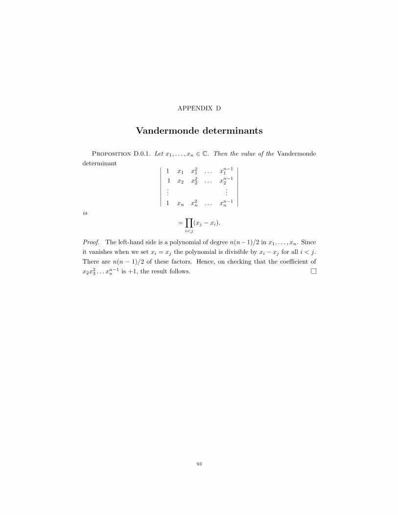
APPENDIX D

Vandermonde determinants

Proposition D.0.1. Let x1, . . . , xn ∈ C. Then the value of the Vandermonde

determinant ∣∣∣∣∣∣∣∣∣∣1 x1 x2

1 . . . xn−11

1 x2 x22 . . . xn−1

2

......

1 xn x2n . . . xn−1

n

∣∣∣∣∣∣∣∣∣∣is

=∏i<j

(xj − xi).

Proof. The left-hand side is a polynomial of degree n(n−1)/2 in x1, . . . , xn. Since

it vanishes when we set xi = xj the polynomial is divisible by xi − xj for all i < j.

There are n(n − 1)/2 of these factors. Hence, on checking that the coefficient of

x2x23 . . . x

n−1n is +1, the result follows.

93

algebraic number theory ben green

Documents