Algorithms for Ray Tracing

by

Karen Dawn Zeitler

A thesispresented to the University of Waterloo

in fulfillment of the thesis requirement for the degree of

Master of Mathematics in

Computer Science

Waterloo, Ontario, 1987 ®Karen D. Zeitler 1987

Author’s Declaration

I hereby declare that I am the sole author of this thesis.

I authorize the University of Waterloo to lend this thesis to other institutions or individuals for the purpose of scholarly research.

I further authorize the University of Waterloo to reproduce this thesis by photo­copying or other means, in total or in part, at the request of other institutions or individuals for the purpose of scholarly research.

(Ü)

Borrower’s Page

The University of Waterloo requires the signatures of all persons using or photo­copying this thesis. Please sign below, and give address and date.

(in)

Abstract

Ray tracing is a technique used in computer graphics to produce very realis­tic images by simulating the passage of light through an environment. With this method, reflections, transparency, shadows, and various blurred effects are easily produced.

To date, ray tracing has generated images of the highest quality. However, the algorithm is computationally expensive. For this reason, many techniques have been developed to reduce computation time. As well, a variety of parallel architectures including vectorization, pipelining, and multiprocessor systems has been proposed. Unfortunately, very few of these designs have been implemented because aspects of the parallelization limit the efficiency of the system. Also, the parallelism often restricts the number of features and acceleration techniques common in sequential ray-tracing systems that can be incorporated into parallel ray-tracing algorithms. Most of these issues have not been considered in any of the proposals.

In this thesis, a description of algorithms developed for ray tracing is presented, with emphasis on the various parallel architectures. Issues that must be addressed before parallel architectures become feasible for implementing ray tracing are identified. Based on these issues, the designs are analyzed and con­clusions are drawn about the suitability of each for ray tracing.

(iv)

Acknowledgements

This research was performed under the supervision of Dr. Kellog Booth in the Computer Graphics Lab at the University of Waterloo. Faculty readers of this thesis were Dr. Kellog Booth, Dr. Ron Goldman and Dr. David Taylor. Dave MacDonald of the Graphics Lab served as the student reader.

I would like to thank all my readers for the care taken in reading the thesis and for their valuable comments.

Financial support from the Natural Sciences and Engineering Research Council (NSERC) and the Computer Graphics Laboratory is gratefully acknowledged.

During my two years at Waterloo, I made many friends who all helped in one way or another. Thanks for being there and for putting up with me, especially in the last couple of months!

Finally, I would like to thank my parents for all their support and encouragement.

Karen Zeitler University of Waterloo December 1987

(v)

Chapter 1

Introduction

Ray tracing is a rendering technique used in computer graphics to create very realistic images [Whit80]. Since the detailed algorithm was introduced to the graphics community by Whitted in 1979, the technique has become exceed­ingly popular for image generation. Of all rendering methods, ray tracing models the widest variety of effects and produces images exhibiting the greatest realism. Reflections, transparency, and shadows are easily simulated by the basic algorithm. With a simple extension, blurred phenomena including depth of field, motion blur, transparency, gloss, and penumbras can also be modeled. In addition to producing very high quality images, the algorithm is simple, yet elegant.

Ray tracing works by simulating the passage of light through an environ­ment in which the complicated interactions of light rays with the objects in the scene are followed. A ray of light is traced from the viewpoint through a pixel on the image plane into the scene. When the ray strikes an object, this object is the visible surface and is used to colour the pixel. To calculate the intensity of the point on the surface, an appropriate illumination model is applied. Shadows are modeled by creating a shadow ray in the direction of the light source. If this ray is blocked by any object, the point is in shadow. At a ray-surface intersec­tion, up to two new rays are generated and traced: one in the direction of reflec­tion to simulate reflectivity and one in the direction of refraction to simulate transparency. Each of these rays is traced recursively, with their intensities accumulated for the pixel. Thus, surfaces with specular properties are easily modeled, while dull surfaces with no specular properties are not accurately ren­dered.

Although ray tracing produces realistic images, the method is very expen­sive to use, especially in its basic form. As well, since ray tracing was first intro­duced, many features which increase this computational expense have been added. Because of the long processing times required to generate even a single image, much research into accelerating the algorithm has been done, with most

1

2

techniques designed in software to execute on a single processor. However, because of the nature of the ray-tracing algorithm, a variety of parallel architec­tures have also been proposed to reduce ray tracing time.

With these architectures, parallelism has been introduced by reordering the computations of the ray-tracing algorithm so that certain aspects are performed in parallel. These architectures fall into three basic classes. The first is vectori- zation, where an operation can be performed on all elements of a vector simul­taneously. Pipelining, in which data is passed through an ordered set of stages operating concurrently, is the second. Finally, multiprocessor systems, in which processors are assigned either a region of image space or a region of object space, have also been proposed.

However, very few of these architectures have been implemented because of practical considerations involving the designs. As well, all execute very simple ray-tracing algorithms in which few features or uniprocessor acceleration tech­niques are included.

In this thesis, an extensive survey of ray-tracing techniques is given, with emphasis placed on parallel architectures designed for ray tracing. Specific features and acceleration techniques that should be included in a ray-tracing sys­tem are identified to allow a comparison of the suitability of each architecture. When parallel architectures are designed in the future, these considerations will have to be addressed.

Chapter 2 gives an overview of ray tracing, describing the basic algorithm as popularized by Whitted as well as the subsequent developments that have improved the quality of images. A variety of primitives for which the ray-object intersection can be solved are used to describe the scene. To increase the visual complexity of the image, primitives can be texture- or bump-mapped. Better sampling techniques can be used to reduce the number of aliasing artifacts that appear. With a simple extension to the basic algorithm, an entire range of blurred phenomena can be produced. Finally, methods of improving the shading of diffuse surfaces have been proposed. For many of these developments, previ­ous attempts to model the phenomenon are mentioned.

Chapter 3 discusses the cost of ray tracing when the additional features are incorporated into the algorithm. Software methods as well as parallel hardware architectures have been proposed for reducing ray tracing time. Various software algorithms to accelerate ray tracing are discussed. Some of the most

3

commonly used algorithms simplify the ray-object intersection test or reduce the number of objects that must be intersected with a ray. Other techniques exist that reduce the number of rays traced or attempt to use ray coherence.

In Chapters 4 and 5, hardware solutions proposed for accelerating the com­putations are examined. Vectorization, pipelining and multiprocessor systems are discussed and specific designs are surveyed. Although the introduction of parallelism accelerates the algorithm, the efficiency of the system is often limited by practical considerations, which are often not addressed in the design. Such considerations are discussed in these chapters. Specific features and software acceleration methods implemented for a uniprocessor ray-tracing system are still essential for a parallel ray-tracing algorithm. Because the architectures employ parallelism in different ways, the division of the computations may make it diffi­cult or impossible to implement certain of these techniques within the design. Once again, many of these considerations have not been addressed in any of the proposals. Chapter 4 deals with parallel architectures in general, while Chapter 5 discusses issues dealing specifically with the more promising multiprocessor architectures.

Finally, Chapter 6 summarizes the developments in ray tracing, with emphasis placed on the parallel architectures proposed for implementing the algorithm. Recommendations about the future of ray tracing and the use of parallel architectures are made.

Chapter 2

An Overview of Ray Tracing

The synthesis of realistic images is one of the primary goals in computer graphics. Consequently, a great deal of research has been directed toward developing and improving rendering techniques. To date, ray tracing [Whit80] has produced the highest quality images with the most realistic effects.

The basic algorithm for ray tracing is simple, yet elegant in its attempt to model the optical geometry of light passing through a scene. Light enables an eye or a camera lens to form an image of the scene before it and gives colour to the materials from which objects are made. Rays of light are emitted from light sources and interact in a complicated manner with nearby surfaces. When light strikes a surface, it reflects in many different directions with a wavelength or intensity that determines the perceived colour of the point on the surface. If the surface is highly reflective, a large portion of the incident light will be reflected about the mirror direction and if the surface is transparent, some light will be transmitted through the surface. Properties of the surface material are also important in determining how the light will interact with the surface. Any rays of light that reach the eye or camera lens will form part of the image of the scene.

Ray tracing attempts to simulate this physical process by tracing rays of light and following their interactions with the objects in the environment. When a ray intersects a surface, the intensity of the point on the surface is calculated and up to two new rays are generated: one in the direction of specular reflection and another in the direction of refraction. Each of these rays is then traced.

Since light in the environment originates at the light sources, one might attempt to trace rays from each light source into the scene. As the rays intersect surfaces, the intensities of all rays leaving the surface would be calculated. Then, any rays that emerged from the scene at the viewpoint would be used to colour a portion of the image. However, a simulated light source must emit an infinite number of rays to model light radiating in all directions from a real

4

5

source of light. As an approximation, many rays sampling all directions about the light source would have to be generated. After the rays interact with object surfaces, even more rays will be produced which must also be traced. Of all of these rays generated, only a very small fraction will ever end up at the viewpoint. If rays were traced from light sources to the viewpoint, much time would be spent tracing rays that contribute nothing to the final image. Hence, to generate images, rays are actually traced from the viewpoint back into the scene.

2.1. Basic Ray TracingThe standard ray-tracing algorithm as popularized by Turner Whitted

[Whit80] is very simple. An imaginary transparent rectangular grid onto which the image will be projected is placed between the viewpoint and the scene. Squares on this image plane correspond to pixels of the screen which will eventu­ally display the image. One at a time, rays are generated from the viewpoint through the centre of each square into the scene. Consider one such ray, called a primary ray. The first object that is encountered by this ray is the visible sur­face for the pixel. To determine the intensity of the intercepted point on this surface, an appropriate illumination model is used. Should a primary ray pass through the scene without striking any surface, it is checked to determine if it is aimed at a light source. If so, the colour of the light source will be use to colour the pixel. Otherwise, the colour of the background is used.

To model reflectivity and transparency, additional rays are generated in the directions of reflection and refraction and traced recursively, with their com­puted intensities accumulated into the final intensity for the pixel. The direction of the reflected ray is assumed to be the specular direction, calculated by observ­ing that the angle of incidence is equal to the angle of reflection. The direction of the refracted ray is computed using Snell’s law, which states that this direction is dependent on the angle of incidence and the index of refraction for the surface material.

Shadows are generated by realizing that a point on a surface is in shadow with respect to a light source if an object is between the point and the light source. Then, the light is obscured by this object, thus casting a shadow. To model this with ray tracing, a shadow ray is generated from the point of inter­section in the direction of each light source. If any object is intersected before this ray reaches the light, the point must be in shadow with respect to that light

6

source. Of course, the same point may be illuminated by another light source.From the ray-tracing process, Whitted generates a binary ray tree in which

branches represent rays of light and nodes represent the closest surface inter­sected by the incoming ray. Branches leaving a node correspond to the rays generated in the directions of reflection and refraction. Leaf nodes represent surfaces that are not reflective or refractive, or rays that pass out of the scene. When shadow rays are traced to the light sources from an intersection point, the results of the tests are associated with the node representing the surface. To accumulate the intensity for the pixel, this tree is later recursively traversed, with the intensities at each node accumulated.

In practice, a ray must be tested for intersection with each object in the scene to determine which objects it strikes. If a ray intersects an object in more than one place, the first intersection is used as the intersection point for the object. By fmding the object with the closest intersection point, the visible sur­face is determined. A ray, r, in three-space is a directed line segment with an origin and direction, and is represented as a parametric equation of the form: r = at 4■ b . Thus, the closest intersection point is the one with the smallest positive value of t. An intersection point is generated by calculating the intersec­tion of the ray and the object. If the two do intersect, the value of t for the intersection is returned, and the intersection point can be calculated.

The algorithm in Figure 2.1 illustrates a simple ray-tracing procedure. Rather than generating the ray tree, recursion is used to accumulate the inten­sity for a pixel.

2.2. Realistic ImagesRealism in computer-generated images is produced through the use of some

well-established techniques. These include colour, illumination models, shading algorithms, visible-surface determination and perspective. Ray tracing also takes advantage of these techniques. Perspective is achieved by tracing the rays through the grid representing the screen onto which the image will be projected. Pixels are shaded using an illumination model and the visible-surface calculation is performed by rinding the first surface that the ray strikes.

Other phenomena, such as shadows, reflection, and transparency, are neces­sary for realism, but are not easily rendered with traditional rendering methods. In these graphics packages, primitives undergo various transformations before

FOR (each pixel)create primary_ray through centre of pixel intensity = Render (primary_ray) store intensity in frame buffer

END FOR

FUNCTION Render (ray)intersect ray with all objects to find closest IF (no object intersected)

RETURN (background_polour)ENDIFintensity = ambient_intensity FOR (each light source)

create shadow_ray in direction of light source intersect shadow_ray with all objects to find blocking IF (no object intersected)

intensity + = Ilium (ray, object, light_source) ENDIF

ENDFORIF (object is reflective)

create reflected_rayintensity + = reflection_coejf • Render (reflected_ray)

ENDIFIF (object is refractive)

create refracted_rayintensity + = refraction_poeff • Render (refracted_ray)

ENDIFRETURN (intensity)

END Render

Figure 2.1 Basic Ray-Tracing Algorithm

8

being scan-converted into the frame buffer [Suth74]. However, these effects are all included in the basic ray-tracing algorithm. In addition to these effects, more difficult fuzzy phenomena, including penumbras, gloss, translucency, motion blur and depth of field, can be reproduced with ray tracing. These effects will be discussed later in this chapter.

While ray tracing easily captures these phenomena, the algorithm does not adequately calculate the illumination for diffuse surfaces, surfaces which are dull or matte. Only an approximation is obtained because secondary rays are not traced from diffuse surfaces, even though light striking such a surface is reflected in all directions.

A major difference between ray tracing and traditional rendering methods is that ray tracing models some of the complex lighting environments in a scene. That is, the algorithm uses global illumination information rather than relying solely on local information as is done in traditional rendering algorithms. Local illumination information consists of only the normal to the surface and the direc­tions to the light sources. Global information refers to information about the environment around the point, such as nearby objects that reflect and refract light, which will affect the colour of this surface. Ray tracing models some of these global effects by tracing rays in the directions of specular reflection and refraction, allowing nearby objects to possibly colour the point. However, since rays are traced backwards from the viewpoint, some of this global information is lost; specifically, light reflecting diffusely from objects in all directions is not accounted for. Also, global information is lost since rays are traced only in the specular directions.

2.3. Early HistoryAlthough ray casting had been performed by computers for many years, the

process was not used for image generation until the late 1960s [Appe68] and early 1970’s [Gold71]. Even then, it was used primarily as a method of hidden- surface removal. In ray casting, individual rays represented by directed line seg­ments are generated and their paths followed until they strike an object. Unlike ray tracing, no more rays are generated after the primary ray intersects the visi­ble surface. The point on the visible surface is then shaded by applying an illumination model.

9

Appel was the first to suggest that rays could be traced backwards from the viewpoint into the scene [Appe68]. Previously, rays were traced from the light sources into the scene and reflected from the surfaces to determine if they emerged at the viewpoint. In his work, ray casting was suggested as a method of automatically shading line drawings for a digital plotter. To represent varying degrees of greyness in an image, the size of the symbol used to fill an area was changed. First, the range of vertex coordinates projecting onto the image plane was determined. Next, a grid of dots representing the resolution of the image was created. A ray from the viewpoint was generated through each dot into object space and the first intersected surface was determined. By tracing a ray from the point on the surface to the light sources, shadows were generated. To optimize the shadow calculation, the need for shadow rays was eliminated by generating shadow outlines.

Goldstein and Nagel from MAGI (Mathematical Applications Group, Inc.) implemented ray tracing in this form to create images shaded with sixty-four lev­els of grey [Gold71]. Their algorithm performed ray tracing from the viewpoint through an imaginary grid of pixels without first projecting the object. Once again, only diffuse reflection was modeled and, although shadows were not simulated, transparent surfaces with no refraction were accounted for as a spe­cial case. Rather than displaying the image on a plotter, they suggested using an intensity modulated CRT.

Ray tracing for image rendering was not further reported until 1979, when Turner Whitted presented his now classic paper [Whit80] and some very impres­sive ray-traced images. From these, ray tracing was recognized as having a legi­timate place in computer graphics. The algorithm that Whitted presented was a simple and elegant solution to many of the shortcomings in then current computer-generated images. Whitted eliminated the special cases needed in the early algorithms and extended ray tracing to model reflective and transparent objects. All subsequent research in ray tracing has been based on Whitted’s paradigm.

10

2.4. Subsequent DevelopmentsSince Whitted first introduced the detailed ray-tracing algorithm in 1979,

the technique has become very popular for image rendering. Consequently, much research has been devoted to the subject, resulting in significant improve­ments to the realism of images. A variety of different primitives can now be used to model scenes to be ray-traced. Surfaces can be texture-mapped and bump-mapped. To reduce aliasing artifacts, new antialiasing methods have been developed. As well, blurred phenomena, often difficult to reproduce, are easily simulated with an extension to the basic algorithm.

2.4.1. PrimitivesVarious primitives, ranging from simple algebraic objects, such as spheres,

to parametric surfaces and procedurally-defined objects, can be rendered with ray tracing. The number of primitives that can be ray-traced is ever growing and new techniques to simplify the ray-object intersection process for all primi­tives are being developed. In order to ray-trace a primitive, the ray-object inter­section must be solvable. Of course, some primitives will have more complicated intersection tests, but as long as the intersection can be solved, the complexity of the primitive and the way in which it is defined are not dominant factors.

Spheres and polygons were some of the first objects rendered because of the simplicity of their ray-object intersection tests. Bicubic patches were handled in the earliest ray tracer by recursively subdividing each patch into polygons [Whit80].

Surfaces can be classified as either implicit or parametric. For implicit sur­faces, points on the surface are found by solving the equation F (x ,y ,z ) = 0, in which F is a function describing the surface. Algebraic surfaces, such as planes, spheres, cones and cylinders are implicit surfaces where F is polynomial and is easily solved. Many algebraic surfaces have been ray-traced [Hanr83, Swee84].

For parametric surfaces, points on the surface are explicitly generated by means of parametric equations that map a set of parameters to a set of points. A curve is defined by an equation in one parameter and a surface by an equa­tion in two parameters. In general, parametric equations describing the ray- surface intersection can be solved in two different manners. If the parametric surface is polynomial, the ray-surface intersection equations can be solved

11

directly, otherwise, numerical methods such as a Newton iteration must be used.Intersections with some parametric surfaces can be solved by first converting

the parametric representations to implicit representations [Sede84, Hanr83]. This is done for a Steiner patch, which is a Bdzier patch defined on a triangle.

Bicubic patches were some of the earliest parametric surfaces ray-traced [Kaji82] and ray intersections with more general parametric surfaces have also been solved using numerical methods [Toth85, Joy86, Barr86].

Deformed surfaces, surfaces created with hierarchical modeling operations that simulate twisting, bending and tapering of objects [Barr84], can also be ray-traced using numerical methods [Barr86].

In addition to these parametric surfaces, surfaces defined by B-splines have been ray-traced directly [Swee86, Swee84]. Previously, such surfaces had to be decomposed into bicubic patches which were then ray-traced.

Recently, an efficient method of ray tracing tessellations has been developed [Snyd87]. Tessellation breaks the surface into many tiny pieces, which then must be ray-traced. Since ray tracing many tiny objects was not previously prac­tical, such intersections were usually solved directly.

Procedurally-defined objects, such as fractals, prisms and surfaces of revolu­tion can also be rendered with ray tracing [Kaji83a]. Fractal surfaces were not previously ray-traceable because fully-evolving the surface before ray tracing generated millions of polygons, which could not be dealt with effectively. How­ever, by evolving during ray tracing only those portions of the surface that are likely to be intersected by a ray, only a small number of polygons is generated at any time [Kaji83a]. A hierarchy of triangular bounding volumes can be created for this purpose. As a variation, the entire surface can be evolved and the hierarchy created before ray tracing begins, but this requires considerable space [Swee84]. Ellipsoidal bounding volumes have since been advocated for enclosing the facets of the fractal surface [Bouv85].

Ray tracing of objects such as clouds, fire, fog and dust is also possible [Kaji84]. These objects have no finite surface, but are represented as densities in a volume grid. Objects created by particle systems [Reev83] also fall into this category.

12

Finally, ray tracing has been used in Constructive Solid Geometry (CSG), in which solid objects are modeled by combining primitives such as blocks and cylinders by means of the Boolean operations union, intersection and difference. Different structuring methods have been proposed to facilitate ray tracing these objects [Roth82, Wyvi86] and vectorization has also been used [Plun85].

2.4.2. Texture and Bump MappingIn computer-generated images, surfaces often appear very smooth because

of a lack of surface detail. Texture mapping, a process that projects a pattern onto a surface, provides added visual complexity in a scene [Blin76, Catm80]. For each point on a textured surface, the corresponding value in the texture map is used to modify the surface colour, usually by scaling the intensity. Bump mapping, an extension to texture mapping, uses values stored in the texture map to perturb surface normals, giving surfaces a wrinkled or rough appearance [Blin78]. Because the intensity of a point depends on the direction of the surface normal, perturbing the surface normal will have the perceived effect of slightly displacing the surface.

Predefined texture map values can be obtained from a digitized image or they can be computer generated. Conceptually, the texture is mapped onto a surface in three-dimensional object space, which is then projected onto the image plane. In scanline algorithms, an inverse mapping is actually performed from the pixel area to the texture map. Since this mapping is rarely one-to-one, a weighted value of the region of the texture map is returned to reduce possible aliasing effects.

A texture or bump map is stored as a unit square and is parametrized by U and V. To index this map, two parameters, u and v, must be generated for the surface at each pixel. For parametrically-defined surfaces, these parameters are known; but for other surfaces, these values must be calculated by relating the x and y values of the point to the boundaries of the surface.

Texture and bump mapping have now been incorporated into ray tracing [Swee84, Ulln83, Dube85]. When a ray intersects a surface that is to be texture- or bump-mapped, a function is applied to calculate the two parametric values, u and v, which index the appropriate texture or bump map. The returned intensity or normal displacement is then used in the illumination function to modify the intensity of the point on the surface. Unlike scanline algorithms that must per­form an inverse mapping from image space back to object space and finally to

13

the parameterized texture map, ray tracing maps directly from object space to the texture map, thereby eliminating the intermediate mapping function.

When texture and bump mapping are combined with ray tracing, images will exhibit additional realism because of the extra detail added to the surfaces. In the ray tracer implemented by Sweeney [Swee84], all primitive objects, including spheres, cylinders, polygons, fractals and B-spline surfaces can be texture-mapped. Texture-mapped fractal mountains are especially realistic.

2.4.3. AntialiasingAs ray tracing is inherently a sampling process, the resulting images may

suffer from aliasing. In the standard algorithm, the scene is sampled by generat­ing a single ray through the centre of each pixel. Aliasing artifacts can appear in many forms, often as staircased edges, disappearing details, or false patterns.

Any area in the image with a marked change in intensity between pixels may show the staircasing effect. High intensity gradients occur at edges of objects and around the edges of highlights and shadows. Disappearing detail will be apparent when primitives or details in the scene are very small and con­sequently are not sampled by any primary rays. Unusual patterns may appear in the image if the scene contains regularly-repeating patterns. Such false pat­terns may be Moiré (swirled curves) or may be a low frequency representation of a pattern that is really of a higher frequency.

If the image being ray-traced is a frame of an animation sequence, these artifacts will be much more noticeable as they move in the final collection of frames. Jagged edges of objects will appear to crawl and tiny objects will ran­domly appear and disappear between frames.

Because the human visual system is very sensitive to aliasing artifacts, some method of eliminating or reducing their appearance is necessary. This technique is referred to as antialiasing.

In rendering packages where primitives are scan-converted into a frame buffer, a variety of techniques is used to antialias lines and edges. Most methods require the use of a filtering technique and were first described by Crow [Crow77, Crow81]. The following discussion deals with sampling and antialias­ing as they have been applied to ray tracing. Since the majority of research into antialiasing techniques in computer graphics has been done for scanline render­ing packages, this is only a subset of the methods that have been developed

14

[Crow81].With ray tracing, a number of techniques have been used to reduce the

effects of aliasing. Supersampling, in which more than one ray is generated for each pixel, is universally applied. The final pixel intensity is then a weighted sum of these samples. Whitted traced rays through each of the four comers of the pixel and averaged the intensity values [Whit80]. By tracing through these grid intersection points on the image plane, additional samples are used for each pixel while still tracing, on the average, one ray per pixel. If this number of samples is not sufficient, each pixel can be further subdivided, thereby changing the resolution of the grid, but requiring more than one ray to be traced per pixel. Adaptive sampling, also used by Whitted, generates additional rays for pixels where there is evidence of intensity changes. Intensity values for adjacent sam­ple points are compared and if there is too much deviation, the pixel is subdi­vided and additional rays are created between the previous sample points.

Since aliasing results from trying to represent a continuous function with discrete values, the addition of more primary rays by using supersampling or adaptive sampling will remove or reduce many of the artifacts. However, super­sampling alone will not correct the problem of a high frequency pattern that incorrectly aliases to a pattern of a lower frequency. A regularly-repeating pat­tern with a frequency greater than the Nyquist limit (half the sampling rate) will always appear as a lower frequency. For this type of aliasing artifact, higher sampling rates improve the quality of the image, but scenes will exist with fre­quencies greater than the Nyquist limit. Since it is not possible to predict the frequency of the pattern that will appear in the resulting image, an adequate sampling rate to remove these artifacts cannot be determined beforehand. In this way, these aliasing patterns result more from using uniformly-spaced sample points than from using too low a sampling rate.

A better sampling method, non-uniform sampling, uses sample points that are not regularly-spaced. With this sampling method, the image becomes more noisy, but the noise can be chosen to be of the “correct” average intensity [Cook86a]. In practice, such noise is found to be less objectionable to the human eye than aliasing artifacts.

Stochastic sampling is a Monte Carlo method that generates patterns of non-uniformly-spaced sample points. Non-uniform patterns are generated in one of two ways: jittered sampling and Poisson disk sampling.

15

The Poisson disk distribution is a non-uniform sampling pattern which closely approximates the non-uniform spacing of photoreceptors found in the human eye. Such a random distribution is basically a Poisson distribution with all sample points separated by a minimum distance. Previous methods for gen­erating this distribution were found to be too expensive [Cook86a], but recently, a method has been developed that easily produces this distribution [Mitc87]. To generate an average of one sample per pixel, sixteen grid points per pixel area are used. A diffusion value based on diffusion values calculated for all previous points and a noise source is generated for a grid point. The algorithm is modi­fied to select as sample points about one in every sixteen grid points while the rest are perturbed by a random amount based on the diffusion coefficients. This method is based on techniques used in the Floyd-Steinberg half-toning algorithm [Floy75].

With jittered sampling, a pixel is divided into subpixels by means of a rec­tangular grid and a sample ray is generated for each subpixel. Instead of tracing the ray through the centre of the subpixel, the sample point is jittered by adding a random perturbation, moving it from the centre. In reality, this is performed by taking a random displacement in each direction from one comer of the sub­pixel. Thus, every point within each subpixel has an equal probability of being chosen as the sample point, resulting in a uniform distribution of sample points across the pixel. While jittering produces an adequate non-uniform sampling pattern, the image may be quite noisy. Scenes sampled with this pattern exhibit more noise than those produced by using Poisson disk sampling. However, it has been shown that jittering a rectangular grid produces a sampling pattern very close to that of a Poisson distribution [Cook86a]. As well, generation of the sample points is inexpensive.

By combining adaptive sampling with stochastic sampling, regions with high intensity changes can be adaptively supersampled. A measure of difference must be determined before more samples are added. An error estimate can be used and more samples generated until the variance of the samples is below a certain amount [Lee85, Dipp85]. Mitchell uses knowledge of the visual system’s ability to detect errors to determine when to adaptively add more samples. Since the eye’s response to changes in intensity is better approximated by contrast, variance in contrast rather than variance in intensity is used. Also, because the eye has different sensitivities to red, green, and blue colours, these three con­trasts are computed separately and compared to different thresholds [Mitc87].

16

Additional methods have been developed to reduce the effects of aliasing. To avoid losing very small objects, Whitted uses a bounding sphere that is large enough that it is guaranteed to be intersected by at least one primary ray. If a ray strikes this sphere, but not the object inside, adaptive subdivision is per­formed so that object will eventually be intersected.

Cone tracing [Aman84] and beam tracing [Heck84] completely avoid the point-sampling nature of ray tracing. In cone tracing, supersampling each pixel is replaced by tracing a “cone” that represents a bundle of rays [Aman84]. Cones are generated from the viewpoint through each pixel so that the cone is the width of the pixel when it reaches the pixel. In this way, the entire pixel area is covered by the cone and an area of the environment rather than just a single point is sampled.

Intersections between primary cones and primitives are calculated and a list is maintained of the eight closest objects that are intersected. For each object intersected, the fractional amount of the pixel that is covered is calculated. This gives enough information for antialiasing because small objects are always detected and the fraction covered gives a weight for the intensity values.

Secondary cones are generated for each intersection, with the centre line of these new cones pointing in the directions of reflection and refraction. The angular spread of the cone and the distance from the apex to the intersected sur­face are modified using equations similar to those used in optics for lenses.

Unfortunately, cone tracing deals only with polygons and spheres as primi­tives and intersection costs are higher than those for traditional ray tracers.

Beam tracing [Heck84] is similar to cone tracing, but rays form a pyramid instead of a cone. Beam tracing begins by sweeping a single “beam” , the view­ing pyramid, through object space. When the beam intersects an object, an exact solution for the intersection is found. Additional beams are generated in the directions of reflection and refraction, allowing all other polygons that pro­ject onto the visible polygon to be determined. During the beam tracing phase, a beam tree with all intersection fragments is generated. Later, this tree is passed to a renderer which scan-converts the polygons in the beam tree. The advantages of beam tracing are that an exact resolution-independent solution is created in object space and that traditional inexpensive antialiasing methods can be used during scan conversion. For a complete description of the beam tracing algorithm, refer to Section 3.5.1.

17

2.4.4. Blurred PhenomenaRay tracing, in the form introduced by Whitted, easily produces certain

phenomena such as reflections, refractions, and shadows by tracing additional rays after the visible-surface intersection. However, these phenomena are all perfectly sharp, whereas in real life, these and other effects can be blurred. Sha­dows have umbras and penumbras, regions of light and dark around the shadow edges, which make them somewhat fuzzy. A form of gloss, in which reflections seen on an object are hazy, is apparent. Also, surfaces may be translucent and not transparent, so that objects viewed through such surfaces will not appear per­fectly distinct. In addition, objects that move very quickly will appear blurred. Finally, in real life, not all objects are perfectly focused because an eye or cam­era lens has a finite focal length, resulting in objects in front of or behind the focal point being blurred. Only a few of these phenomena have been reproduced with other rendering methods.

In traditional ray tracing, all phenomena are very sharp because ray direc­tions are calculated precisely. Ray tracing simulates the image that would be produced by a pinhole camera so that every object is in focus and primary rays are generated through the centre of each pixel at a single instant of time. At surface intersections, directions of reflected and refracted rays are determined exactly and secondary rays are followed only in these specular directions. Finally, lights are modeled as point sources so a point on the surface cannot be partially illuminated by a light.

Distributed ray tracing, a simple extension to the traditional algorithm, correctly produces gloss, translucency, penumbras, motion blur and depth of field [Cook84]. With this method, blurring is achieved because directions for rays are no longer fixed, but rather, are chosen stochastically. For each effect, the direction of a sample ray is perturbed slightly according to a distribution function describing the phenomenon.

To correctly approximate the final intensity of a pixel, integrals should be taken over a number of variables, including the pixel area, the lens area, the directions of reflection and refraction, the light source area, and time. In gen­eral, these variables of integration can be regarded as additional dimensions to be sampled. By stochastically distributing rays that sample each of these dimen­sions, distributed ray tracing performs a Monte Carlo evaluation of each of these integrals. Just as stochastic sampling generates rays to sample the pixel area, distributed ray tracing stochastically samples each of the other dimensions.

18

If traditional ray tracing rendered these phenomena, additional rays would have to be generated to sample each of the dimensions, with the final pixel intensity calculated by weighting the results of the rays traced to sample each phenomenon. However, this is extremely expensive because the number of rays traced is magnified by the number of phenomena being modeled. When sto­chastic sampling and distributed ray tracing are combined, no more rays than those needed to oversample in space are necessary. Thus, the advantage of dis­tributed ray tracing is that more rays are not added to model each phenomenon, but existing rays are perturbed in each dimension.

Blurred reflections are a form of gloss [Hunt75] that is observed in mirrored surfaces. The amount of haziness observed depends upon the fraction of light reflected and the angle of spread of the reflected light about the direction of specular reflection. Rather than generating a single ray in the mirror direction, secondary rays are distributed about this direction through jittering according to the specular distribution function. Gloss has not previously been produced by any other rendering method.

Translucency, a blurred transparency, results from diffusion of light as it passes through the surface, and as such, is the opposite phenomenon from gloss. Objects observed through a translucent surface will not be distinct. In distri­buted ray tracing, translucency is produced by distributing refracted rays about the direction of specular refraction according to the transmittance function. While transparency has been produced by other rendering methods, translucency has not been addressed.

Penumbras are fuzzy shadows that are created when a light source is par­tially obscured by an object in the scene, with the diffuse intensity of the point on the surface proportional to the solid angle of the visible area of the light. In the ray tracing solution, rays are distributed over the area of the light source, so that some rays will be blocked while others will not. The probability of tracing a ray to a particular location on the light source is proportional to the intensity and projected area of that location.

The shadow buffer [Will78] produces the effect of penumbras as a result of antialiasing. In this algorithm, the scene is first rendered from the view of the light source, creating a shadow buffer that indicates whether the point is in sha­dow with respect to that light source. Later, this information is used when rendering the scene from the viewpoint. In addition, the Cook-Torrance reflec­tance model includes a term for attenuating surface intensity by the fraction of

19

the visible hemisphere blocked by other objects [Cook82]. However, this term is never calculated in the implementations reported in the literature.

Motion blur appears as blurred images of objects that move quickly during the time of the frame. In computer graphics, pictures are usually generated at a single instant of time, conveying little impression of motion if objects are mov­ing. To produce the effect of motion blur in distributed ray tracing, rays must be distributed over time, effectively taking samples at different times. Because all that is required is to determine the positions of the viewpoint and the objects at any time and not to trace additional rays, this method is simple. As well, intersections, shadows and reflections will all be correctly motion-blurred.

Motion blur is a phenomenon that is not easily produced by other rendering methods, although solutions have been proposed. Two methods were suggested by Korein and Badler [Kore83]. In the first method, object movement is approximated by a continuous function that first determines how long each object covers each pixel, then performs hidden-surface removal, and finally cal­culates the intensity. In the second method, additional samples are taken during the frame time and the resulting intensity function is filtered to generate blurred multiple exposures.

Another method uses a sophisticated camera model and equations that describe the relationship between object position and image points given object speed, direction, and exposure time [Potm83]. Hidden-surface removal is per­formed first and the resulting image intensities are blurred in a postprocess.

Motion blur is simple to produce for fuzzy objects created with particle sys­tems [Reev83] in which primitive objects are modeled as clouds of stochastically-generated particles that are bom, have a lifetime, and die. Attri­butes of particles include their velocity and direction. By calculating a particle’s position at the beginning and middle of a frame, an antialiased line can be drawn between the two points, producing a streaked image.

In another algorithm [Catm84], a filter associated with each pixel is used. Motion blur is added by noting that a filter stretched in the direction of motion is equivalent to shrinking the polygon relative to the pixel center in the same direction. After filtering, the hidden-surface problem is solved.

Finally, a method that takes a raster image and blurs it as a postprocess has been suggested [Max85]. Objects are sorted in depth, motion-blurred and then composited to form the final motion-blurred image. Images and masks are all

20

originally created at a single instant of time, with the raster and mask then motion-blurred and successively combined with a compositing process.

Depth of field, in which some objects in the scene are not focussed, is observed in photographs because lens apertures are finite. Consequently, only objects at the focal point are rendered in perfect focus. If the effects of captur­ing an image with a camera are wanted, this phenomenon will be desirable in computer-generated images. In ray tracing, this effect can be produced by dis­tributing rays over the surface of the lens. First, the focal point for the lens is calculated by tracing a ray from the viewpoint through the point on the pixel. Then, the focal point is located at the midpoint of this ray. A point on the lens surface is generated by jittering a pattern of lens locations and a primary ray is traced from this point through the focal point and through the pixel.

Some work in producing depth of field effects has previously been done. In a sophisticated camera model that describes the effects of lens and aperture, depth of field is produced by a postprocess [Potm82]. As well, depth of field can be produced in the same filtering approach that simulates motion blur [Catm84], with the filter scaled relative to the polygon’s distance from the focal plane.

In distributed ray tracing, rays are generated in a direction with a certain probability corresponding to a filter, thereby performing a Monte Carlo evalua­tion of the integral in that dimension. By combining distributed ray tracing with stochastic sampling used for antialiasing, all perturbations are applied to each ray rather than to additional rays generated to sample each dimension. The number of rays required does not depend on the number of dimensions, but depends instead on the variance of the intensity of the image [Lee85]. There­fore, no more rays than those necessary to supersample object space are needed.

The basic algorithm for distributed ray tracing is as follows. The location on the pixel for the primary ray is determined by jittering a rectangular grid. Next, the time for the ray is selected and all objects are moved to their correct positions. To model depth of field, the focal length for the lens at that screen location is calculated, a position on the lens is selected, and a primary ray is generated from this position through the focal point. At an intersection with the visible surface, a shadow ray is traced to a location on the light source. For a mirrored surface, the direction of the reflection ray is chosen by jittering direc­tions selected from the reflectance function. A refracted ray is then generated in a similar manner.

21

When directions of sample rays modeling different phenomena are chosen completely at random, the resulting image tends to be very noisy because sam­ples can cluster. Therefore, jittered sampling can be performed in each of these other dimensions to ensure that the primary rays of a pixel sample the entire range of values describing each phenomenon [Cook86a]. Just as one primary ray samples a portion of the pixel area, it then samples part of the range describ­ing each additional phenomenon.

A table whose entries associate a range of sample values with the screen space location of a primary ray sampling the pixel is created for each phenomenon being modeled. Once the correct range for a ray is selected from this table, the exact location for the sample ray is calculated by jittering. Con­sider a pixel stochastically sampled by four primary rays. Each of these rays and its descendants is labeled by the number of the pixel quadrant through which the primary ray passes. This can be visualized with the following table, corresponding to the area of the pixel:

Similar tables, whose quadrants are associated with a range of sample values, are created for other dimensions that will be sampled by the four rays. The label given to the primary ray serves as an index into this table, thereby mapping a range of values to a location of the ray in screen space. Because each of these tables has the same number of entries as the number of primary rays sampling a pixel, each primary ray will sample a different region of the function describing the phenomenon.

However, now that tables determine, in part, the location of a sample asso­ciated with a particular primary ray, care must be taken that there is no correla­tion between samples from different dimensions. If a primary ray passing through a particular quadrant of the pixel always sampled the same range of another phenomenon, the rays would be correlated, resulting in possible aliasing. Therefore, each group of primary rays should randomly sample different ranges of each phenomenon. To achieve this, entries in each of the tables are randomly generated for each phenomenon at each level of recursion. To avoid any corre­lation between pixels, different tables should be generated for each successive

22

pixel.The different tables can be generated when needed and then saved during

the tracing of the first ray from a pixel and later used by the other rays belong­ing to the same pixel. However, this requires considerable storage and is unnecessary as long as the corresponding rays use the same permutation of the table.

Tables created for motion blur and depth of field are used by the primary rays sampling the pixel and can simply be generated and saved. However, tables for the gloss, translucency and penumbras are treated differently because they must be generated whenever new rays are traced from an intersection. Corresponding rays from the four different ray trees, however, must use the same table. For these tables, a random sequence of all possible permutations is generated and saved in a single permutation table, with the correct permutation determined by indexing into this table. If each ray-object intersection generates two secondary rays, the resulting ray tree would be a full binary tree whose nodes are easily numbered. At each node, a maximum of three tables is needed: one for gloss, one for translucency, and one for penumbras. Therefore, these tables can also be numbered by knowing the associated node number in the binary tree. It is this number that is used by a ray to index into the permutation table.

Then, a ray needing the sample range for a particular phenomenon uses the node number of the binary tree and the phenomenon being modeled to deter­mine the correct permutation table index. The corresponding permutation table is generated and the correct range selected using the ray label.

When all primary rays through one pixel have been traced, a new random sequence of permutations is generated for the next pixel.

Cone tracing, originally developed for antialiasing and described in Section 2.4.3, can be used to produce fuzzy shadows, dull reflections and translucency by broadening the cones of light that are traced [Aman84]. To produce penum­bras, the shadow ray is broadened to the diameter of the light source and the fraction blocked by intervening objects is calculated. Gloss is produced by broadening the reflected ray and translucency is produced by broadening the refracted ray.

23

2.4.5. Illumination of Diffuse SurfacesRay tracing can reproduce many phenomena that result from global illumi­

nation in the environment. Complex interactions of light within a scene are modeled by tracing rays from the visible surface to include the contributions of other objects to the illumination of a point. With standard ray tracing, reflection and transparency of specular surfaces are easily modeled. With distributed ray tracing, additional fuzzy effects such as penumbras, gloss, translucency, depth of field and motion blur can be generated.

Despite producing images of very high quality, ray tracing still does not adequately treat the shading of diffuse surfaces. These surfaces, which are dull and matte, have little or no specular component. In a realistic environment, many surfaces may be diffuse, including painted walls, fabric, paper and wood. Light striking a diffuse surface is reflected in all directions so that illumination of the surface from any direction contributes to the intensity. However, standard ray tracing will follow rays from a surface only if it is reflective or refractive, and then only in these specular directions. Distributed ray tracing gives a slightly better approximation for this illumination because rays are distributed about the principle angles of reflection and refraction. For diffuse surfaces, how­ever, the specular direction gives little indication of where additional sources of illumination may be found.

Ray tracing, like most shading models, accounts for illumination from secondary light sources as ambient light, global illumination that is constant throughout the environment. Each object, of course, reflects a different amount of ambient light. With ray tracing, the contribution of light reflected or transmitted by other surfaces is partially modeled by tracing rays in the direc­tions of reflection and refraction. The effects of secondary illumination on dif­fuse objects is approximated with the ambient term. However, an ambient term is not sufficient for diffuse surfaces.

In effect, ray tracing provides only an approximate solution to the calcula­tion of illumination throughout an environment, which is accurately described by Goral [Gora84] and Kajiya [Kaji86J. The light reflected from a point on a sur­face is dependent on all light arriving at that point from every direction above the surface. In this way, the calculation of the outgoing intensity requires an integration over the entire hemisphere above the surface. Both Goral and Kajiya base their equations on radiation heat transfer theory from thermal engineering [Sieg81, Spar78].

24

The radiosity method [Gora84] uses these equations to describe the transfer of energy between diffuse surfaces in an enclosure. With this method, the inten­sity of light leaving a diffuse surface is a function of self-emitted energy and all energy incident upon the surface. This incident energy is, in turn, dependent upon the energy leaving all other surfaces in the environment.

The “rendering equation” described by Kajiya [Kaji86] expresses these ther­mal conservation of energy equations in a form more suited to computer graph­ics. As well, surfaces are not restricted to being ideal diffuse reflectors. Ray tracing is shown to be an approximate solution to this general lighting equation, where only the specular energy is taken into account.

Two different phenomena associated with the shading of pure diffuse sur­faces are neglected by ray tracing: the illumination of such surfaces by secondary light sources (objects that are highly reflective or transparent and transport light) and colour bleeding, in which a diffuse surface acquires some illumination from another nearby diffuse surface. As these two effects are associated with dif­ferent shortcomings in the algorithm, they are often handled separately.

Secondary light sources are very important to the shading of diffuse sur­faces. When light from a primary light source strikes a very reflective or refrac­tive surface, the light is transported with almost full intensity. Hence, this sur­face becomes an additional source of light in the environment. After additional bounces, light would be attenuated, resulting in weaker secondary sources. For ideal diffuse objects, the only light leaving the surface is diffusely reflected. The diffuse component is calculated using Lambert’s Law, which states that the reflected intensity falls off as the angle between the direction to the light source and the surface normal increases. In ray tracing, diffuse contributions are calcu­lated only for each primary light source.

However, for some diffuse surfaces, the main source of illumination may come from secondary light sources. Consider a pure diffuse surface that is in shadow with respect to the only primary light source. In this case, secondary light sources that illuminate a point on the surface can make a substantial contri­bution to the perceived intensity. If a mirror reflects light specularly from the light source onto the surface, the point will be illuminated indirectly by the light source. However, the diffuse component for the surface will be zero because the shadow ray aimed at the light source is blocked. The mirror is a secondary light source.

25

Consider the same diffuse surface indirectly illuminated by a transparent sphere that transmits light directly from the light source. However, once again, the diffuse component will be zero because the shadow ray strikes an object before reaching the light source. This suggests that shadows cast by refractive objects must be treated differently from those cast by opaque objects. Following the shadow ray through multiple refractions is not beneficial because it will prob­ably not emerge at the light source. Transparent objects may actually cause light to focus on a surface creating an interesting pattern of illumination and shadow. In graphics, this effect is known as “caustics” [Kaji86], although the term originates in optics, where it refers to a curved surface illuminated by light rays that have been focussed by a lens [Bom59].

Ray tracing does not account for these effects because rays are traced back­wards from the viewpoint into the scene rather than from the light sources. If rays were traced in the opposite direction, contributions from secondary light sources would be accounted for automatically as these rays interacted with objects in the environment. However, tracing rays from the light sources is too costly because rays would have to be sent in an infinite number of directions from each light. As well, very few of these rays would eventually emerge at the viewpoint to contribute to the image.

Colour bleeding between two diffuse surfaces is another phenomenon that ray tracing does not reproduce. If two diffuse surfaces are very close, light rays will reflect from one surface onto the other. In this way, a surface will acquire some colour from the second by means of this diffuse reflection. Standard ray tracing does not capture this interaction between the diffuse surfaces because no additional rays are traced after the intersection with the visible surface.

Several modifications have been proposed to the ray tracing algorithm to account for these deficiencies. Some will correctly handle indirect illumination, some colour bleeding, and a few both.

The problem of illumination by secondary light sources has been investi­gated by several researchers [Heck84, Arvo86, Inak86]. Two of them propose tracing rays from the light sources as a preprocess. Beam tracing [Heck84], in which beams of light are traced as a unit from the viewpoint, can trace beams from the light sources as a preprocess before beam tracing begins to render the scene. When these light beams intersect objects in the environment, polygonal areas of illumination on the surfaces are formed. If the surfaces are reflective or refractive, the object becomes a secondary light source and the intensity

26

information for the illuminated polygon is stored in the data base as additional detail. Light beam tracing continues with the beam fragmented and redirected in the directions of reflection and refraction. During beam tracing to render the scene, this stored intensity information is added to the calculated intensity. The complete beam tracing algorithm is described in Section 3.5.1.

In the same way, rays can be traced from light sources as a preprocess [Arvo86]. During the preprocessing, rays are generated at each light source and the energy deposited on the surfaces is accumulated in an illumination map for each surface. After light rays are traced, each map contains the intensity of illumination of the surface by secondary light sources. When ray tracing is per­formed, the intensity from the illumination map for the surface is added to the diffuse component for the surface.

Another method using lens equations can produce some of the same effects [Inak86]. These formulas are used to determine the intensity of light transported from convex lenses through reflection or refraction. Ratios of the initially illuminated area and the area illuminated after reflection or refraction are calcu­lated using the focal length of the lens. From these ratios, the intensity of the illuminated area on the diffuse surface is easily determined. However, this method is only applicable to spheres and each sphere must be tested to deter­mine if it transports light to the diffuse surface.

Dubetz also attempted to solve the problem of indirect illumination of dif­fuse surfaces [Dube85]. Instead of tracing rays from the light sources, diffuse surfaces are treated by tracing secondary rays in many directions about the sur­face. These rays are stochastically distributed in an imaginary sphere placed on the surface at the intersected point, with ray directions chosen so that all areas of the scene are sampled equally. Any intensity found with these sample rays is added to the diffuse component of the intensity of the surface. Distributed ray tracing is used to statistically alter the directions of the chosen rays and to reduce the number that must be traced.

Results indicate that colour bleeding effects are adequately modeled, but statistically, many rays must be traced to produce the correct illumination from nearby diffuse surfaces. Unfortunately, this method does not properly account for secondary illumination by highly reflective or refractive surfaces because it is possible that no rays sample the secondary light source.

27

Modifications to the distributed ray tracing algorithm allow Kajiya to solve the equation describing illumination in an environment [Kaji86]. As a conse­quence, the effects of the illumination of diffuse surfaces by secondary light sources and colour bleeding are produced.

Rather than generating a branching tree at each ray-surface intersection, “path tracing” follows only one ray, either in the direction of reflection or refraction. In effect, this selects a path through the tree which would have been generated with the traditional algorithm. Because primary rays contribute more information to the shading of the pixel than secondary rays, many primary rays are generated and little is lost by following only one ray at each subsequent intersection point.

The correct proportion of reflected and refracted rays is maintained through variance reduction techniques. The number of each type of ray sent is recorded and the probabilities of choosing each are continuously updated so that the desired distribution is matched. In total, enough incoming directions are sam­pled for each pixel that the intensity of the diffuse component for the surface is accurate. These modifications have adequately shaded diffuse surfaces by accounting for indirect illumination by secondary light sources as well as the interactions with close diffuse surfaces.

The introduction of the radiosity method [Gora84] made important advances in the accurate calculation of illumination for diffuse surfaces. “Form factors” that specify the fraction of energy leaving one surface and incident on another are calculated for every pair of surfaces in the environment. The expression for the illumination of the surfaces results in a series of equations that must be solved simultaneously. Although form factors are a new idea in com­puter graphics, the concept has been used in radiation heat transfer theory for many years with the coefficients also known under other names, including “con­figuration factors” [Sieg81].

However, the original implementation of the radiosity method dealt only with pure diffuse surfaces in an empty room where occluded surfaces were not considered. Colour bleeding effects were accurately produced. An advantage to this method is that it is view-independent, so the form factors need only be cal­culated once for a static environment.

28

The radiosity method has since been improved to model occluded surfaces and produce shadows. One method uses special shadow interpolation algorithms [Nish85]. A more efficient way of handling occluded surfaces using hemi-cubes was introduced by Cohen and Greenberg [Cohe85].

Textured surfaces have also been rendered [Cohe86]. In addition, the radiosity method has been improved to handle the transmission of radiation through media that absorb, emit and scatter the light [Rush87] and has been extended to non-diffuse surfaces [Imme86]. Directional restrictions can be added to the radiosity equations to account for specular reflection. However, this drastically increases the number of equations that must be solved and serious aliasing artifacts are often present in the resulting images. Because specular reflections produce regions of the image with high intensity changes, the use of too few sample points in the environment is noticeable. Further subdivision requires too much space and computational expense. This is the real downfall of the radiosity method.

Because specular illumination is difficult to handle, Wallace advocates a method of combining the strengths of radiosity with those of ray tracing [Wall87]. In this algorithm, the radiosity method is used as a preprocess to correctly measure the diffuse illumination of a surface and ray tracing is used as a postprocess to calculate the specular component. The addition of the two intensity values determines the correct intensity.

To perform the first pass, the radiosity method is extended to handle diffuse transmission (translucency) as well as specularity to correctly calculate the dif­fuse component. As an alternative to distributed ray tracing, a viewing frustum is created about the directions of reflection and refraction, and rays are traced through each “pixel” . A simple z-buffer algorithm determines the visible sur­face at each pixel. The resulting sample intensities are weighted before being accumulated into the intensity for reflection or refraction.

2.5. Chapter SummaryRay tracing produces extremely realistic images that incorporate a wide

variety of phenomena, including reflections, transparency and shadows. The basic algorithm is elegant in its attempt to simulate the passage of light through an environment. Since the introduction of ray tracing, additional features have been added.

29

Many different primitives can now be used to model the scenes. Such prim­itives include simple algebraic surfaces like spheres and polygons, as well as parametric surfaces with iterative intersection tests. Fractal surfaces and other procedurally-defined objects can also be ray-traced. To add visual complexity to the scene, each of these primitives can be texture- or bump-mapped. Blurred phenomena are included with distributed ray tracing in which ray directions are altered slightly from their normal directions.

Because ray tracing is a sampling process, methods of antialiasing are neces­sary. Supersampling and adaptive sampling are standard techniques. Also, non-uniform sampling methods that jitter regularly-spaced sample locations are used. These methods more effectively eliminate certain types of aliasing artifacts by replacing the artifact with noise of the “correct” average intensity.

Although ray tracing correctly models surfaces with specular properties, illumination of diffuse surfaces is not accurately calculated because rays are not traced from the light sources and because no rays are traced from diffuse sur­faces. Methods within ray tracing to correct the deficiency generally fail on sta­tistical grounds.

Chapter 3

Reducing Ray Tracing Time

While ray tracing produces impressive images, it is computationally very expensive, with a single frame taking anywhere from a few minutes to a few hours to compute. One problem is that coherency cannot be used efficiently for tracing the rays. Each pixel requires a separate tree of rays to be created, and is treated as a completely independent problem. Considering that each image may be only one frame of an animation sequence for which a rate of 24 frames per second is required, the expense of ray tracing is obvious. One of the reasons for the expense is that the computations are in floating point.

The time required to compute a frame depends directly upon the resolution of the image and the number of objects in the scene. Rays must be traced for each pixel and, for each ray, all of the objects must be tested to determine the closest one intersected. Whitted estimates that the greatest amount of time is spent calculating ray-object intersections [Whit80]. The percentage ranges from 75 percent to over 95 percent for a complex scene.

As well, many of the features presented in Chapter 2 which have been incorporated into the ray-tracing algorithm may be very expensive computation­ally. In some cases, additional rays will be traced and in others, ray-object intersection tests will be very complicated. For additional primitives such as sur­faces with iterative solutions, the intersection test will require more time than for simple spheres and polygons. Fractal surfaces, composed of thousands of polygons, require too many intersection tests to ray-trace directly. As a result of antialiasing by supersampling, additional rays are generated for each pixel. Dis­tributed ray tracing requires no more rays than for stochastic supersampling, but directions must be jittered in many dimensions before a ray can be generated and traced. When motion blur is modeled, the viewpoint and objects must be moved to the correct location in time before each ray is traced. To better approximate the intensity of a diffuse surface, methods usually require additional sample rays to be traced.

30

31

Because the computational requirements are very heavy, a great deal of effort has been spent trying to accelerate the process. Bounding volumes are used around objects to simplify intersection testing. Structure has been imposed on the scene to reduce the number of objects which normally would need to be tested for intersection with a ray. Methods are used to control the number of rays traced by limiting the depth of the tree and by minimizing the shadow rays traced to the light sources. Forms of ray coherence have also been tried. In addition, a variety of parallel architectures has been proposed for ray tracing.

This chapter describes only those techniques that are implemented in software. In Chapter 4, hardware solutions to reduce ray tracing time by incor­porating parallelism in the algorithm are discussed.

3.1. Bounding Volumes

Bounding volumes constructed about the objects in a scene have been used successfully to accelerate ray tracing. A bounding volume completely encloses the object and is designed to be much simpler to intersect with a ray than the object itself. Recognizing that ray-object intersection tests can be costly because certain types of objects are difficult to intersect, Whitted placed such bounding volumes about complex primitives [Whit80]. With most ray-object intersection tests replaced by ray-bounding volume intersection tests, the cost of determining an intersection can be greatly reduced. Before a ray is to be tested against an object, it is first tested for intersection with the bounding volume associated with the object. If the ray does not intersect the bounding volume, it cannot possibly intersect the object. However, if the ray does strike the bounding volume, it is probable that it also intersects the object, so only then is the ray tested for inter­section with the object. Objects that are simple to intersect, such as spheres, do not require bounding volumes.

In standard ray tracing, a ray must be tested for intersection with each object in the scene. If such ray-object intersections are expensive because primi­tives are complicated, the time required to perform the large number of intersec­tion tests necessary will be a large portion of the final ray tracing time. Thus, any simplification of the ray-object intersection test is desirable.

Bounding volumes can assume a variety of different shapes. Whitted used spheres primarily because of the simplicity of a ray-sphere intersection calcula­tion [Whit80]. Other bounding volumes that have appeared in the literature are rectangular parallelepipeds [Rubi80, Roth82, Wegh84, Dube85], cylinders

32

[Wegh84], “cheesecake extents” [Kaji83a] and ellipsoids [Bouv85] for fractal surfaces, and “slabs” [Kay86], which bound an object with pairs of planes.

Weghorst, Hooper and Greenberg [Wegh84] have investigated some con­siderations for selecting the shapes of bounding volumes and have identified two criteria as being of prime importance: the tightness of fit of the bounding volume to the object and the cost of the ray-bounding volume intersection test.

Clearly, the more tightly the bounding volume fits the object, the better the bounding volume. If a bounding volume leaves too much space around an object, a ray is likely to intersect the bounding volume while not actually striking the object. However, not until the object is tested for intersection will this be known, wasting a ray-object intersection test. By minimizing the amount of empty area around the object, such calculations can be avoided.

As well as the amount of empty area, the bounding volume complexity must be considered when selecting a shape. If a bounding volume has a com­plex shape, the resulting ray-bounding volume intersection test could be quite costly. Since the purpose of using bounding volumes is to simplify the usual ray-object intersection, the shape of the bounding volume should be made as simple as possible. When the complexity of ray intersections is compared for dif­ferent shapes of bounding volumes, that of the sphere is the simplest. Next is that of an arbitrarily-oriented parallelepiped, and last is that of a cylinder. To determine if the ray intersects a sphere, the sign of the discriminant b 2 — 4ac used to solve a quadratic equation describing the intersection is checked. Test­ing a bounding box for intersection requires finding if the ray intersects each face of the box.

However, there is a tradeoff in the tightness of fit and the simplicity of the intersection calculation. Invariably, bounding volumes that most tightly enclose the object have the most complex intersection calculations. Thus, a bounding volume shape for an object should be chosen to try to minimize both of these cri­teria. Since a bounding volume that is best for one object is not necessarily the best for another, Weghorst, Hooper and Greenberg allow more than one shape of bounding volume for a scene. An optimal bounding volume shape, selected from a sphere, an arbitrarily-oriented rectangular parallelepiped, and a cylinder, is chosen for each object in the scene.

33

Rubin and Whitted [Rubi80] propose the use of arbitrarily-oriented rec­tangular parallelepipeds for enclosing objects. By allowing any orientation of the boxes, the bounding volumes can more tightly surround the object. The orienta­tion of the bounding volume is described by a four by four transformation matrix. Any ray that is to be intersected with the object is first tested for inter­section with the bounding volume. To simplify the intersection operation, the ray is first transformed into the coordinate system defined by the axes of the bounding volume by using this transformation matrix. This type of bounding volume has since been used by Dubetz [Dube85, Dube86].

Roth [Roth82] used a similar but more restrictive set of bounding volumes, requiring the boxes to be aligned with the axes of the world coordinate system instead of being arbitrarily-oriented in space. While simple to intersect with a ray, such bounding volumes leave a large amount of empty space about the objects they bound.

Rectangular parallelepipeds are also used by Weghorst, Hooper and Green­berg [Wegh84]. In their implementation, these boxes are allowed to be oriented arbitrarily but no attempt is made to simplify the intersection test by first transforming the ray into the subspace of the box.

Kay and Kajiya [Kay86] have proposed the use of bounding volumes formed from sets of parallel planes. Unlike parallelepipeds used in other schemes, these bounding volumes are not restricted to being six-sided, but can be constructed from an arbitrary number of pairs of parallel planes, allowing an object to be more tightly enclosed.

Extents are created by specifying pairs of planes. In the plane equation, ax + by + cz + d = 0, the plane normal is specified by a, b, and c, while d fixes the plane in space. By specifying the three coefficients, a, b, and c, a set of planes that are parallel to each other with the same normal can be defined. Two d values, dnear and dfar, will select two of these parallel planes. The space between these two planes is called a “slab” and any three non-parallel slabs define a bounding volume.

By increasing the number of slabs used for the bounding volume, the object can be enclosed more tightly in exchange for a more complex ray-bounding volume intersection calculation.

34

To reduce the storage required to define the extents, plane normals are chosen and stored in advance. Only the two values, dnear and dfar, for each slab have to be stored for each object. Bounding volumes are easily computed for polyhedra, simple implicit surfaces such as spheres, and compound objects.

A ray is intersected with this type of bounding volume by intersecting it with each of the slabs composing the extent. Fortunately, this calculation can be greatly simplified by performing some precomputation based on the fact that plane normals are the same for each object. The final computation cost for each slab of a bounding volume is two subtractions, two multiplications, and one com­parison.

Kajiya [Kaji83a] presents a specialized type of bounding volume, called a “cheesecake extent” , for use in bounding fractal surfaces. This bounding volume is formed by sweeping a triangular facet of the surface by ±7/ in the y direction so that the facet, when fully evolved, will be entirely enclosed by the bounding volume. A cheesecake extent can be created for every facet at each level of subdivision of the fractal surface. Bouville uses ellipsoids to enclose each facet because such volumes better fit the surface [Bouv85]. An ellipsoid is first transformed to a sphere of unit radius centred on the origin to simplify the intersection test.

Thus far, all bounding volumes described enclose an object positioned in three-space at a single instant of time. For most scenes and phenomena, this is sufficient. However, to model motion blur with distributed ray tracing, rays traced during a single frame can occur at any time during the frame. Before rays can be intersected with any of the objects in the scene, the objects must be moved to their appropriate position at that instant of time. If bounding volumes are then created and the ray tested for intersection with the bounding volume, much time can be spent calculating object positions and creating bounding volumes for objects that are never intersected by a ray. To reduce this time, bounding volumes in time can be created for each object in the scene for a single frame [Cook86b]. The position of each object at the start and at the end of the frame are calculated and a bounding volume that encompasses both positions is created. Then, only when a ray intersects this bounding volume is the object moved to the correct position for the time of the ray, and the ray tested for intersection with the object itself.

35

3.2. Structuring the SceneOne of the most promising techniques for accelerating ray tracing creates a

data structure describing the scene to cull many objects from being tested for intersection with a ray. This, in turn, reduces the total number of ray-object intersections that need to be performed. The standard ray-tracing algorithm requires that the ray be intersected with each object in the scene in order to determine the closest object. Structuring the scene description, either by dividing the scene into subvolumes or by placing the objects into a hierarchy, can remove large numbers of objects from consideration for intersection. When designing such a structure, three criteria should be met. First, objects that cannot possibly be intersected by the ray should immediately be culled. Second, objects should be tested for intersection in the approximate order of their distance along the ray. Finally, the closest intersecting object should be determined without need­ing to test additional objects in the scene.

3.2.1. Object HierarchiesOne way to reduce the number of ray-object intersections required for ray

tracing is to decompose the scene into an object hierarchy represented as a tree of bounding volumes. At each node is a bounding volume that encompasses the bounding volumes of its children. Interior nodes represent composite objects or objects that are grouped together, while leaf nodes represent primitives. The hierarchy is created bottom up with only nearby bounding volumes grouped together under a parent bounding volume. Finally, the root node of the hierar­chy contains a bounding volume that encompasses the entire scene and all other bounding volumes.

When a ray is traced, it is first tested for intersection with the bounding volume at the root of the hierarchy. If the ray intersects this bounding volume, it is tested for intersection with the bounding volumes of each child. Any inter­section with a bounding volume requires that the bounding volumes of all chil­dren be recursively examined in the same manner. If a bounding volume is not intersected, the ray could not possibly intersect any bounding volume or object below it in the subtree, so no objects in this subtree need to be tested for inter­section. The search proceeds recursively down the tree, with bounding volumes expanded and tested at each level. Finally, at the leaf level of the tree, the objects are actually tested for intersection and the closest is returned.

36

With this hierarchy, large numbers of objects are removed from considera­tion by traversing only promising branches of the tree.

This object hierarchy can be constructed manually by determining which objects and bounding volumes are near enough to be grouped into a cluster. Another option is to create bounding volumes at each node of a hierarchy that was used previously to model the scene. This is possible because in such hierar­chies, objects used to form parts of more complex objects are often close to each other, resulting in a bounding volume that should be minimal. Finally, the hierarchy can be created automatically from the positions of bounding volumes surrounding the objects. Regardless of how the hierarchy of objects is created, bounding volumes are always generated automatically.

Desirable characteristics for such an object hierarchy are presented by Kay and Kajiya [Kay86]. Only objects and bounding volumes that are near each other in space should be grouped together under a single bounding volume. As well, the size of each bounding volume should be minimal, and the sum of the sizes of all bounding volumes should also be minimal. When constructing the hierarchy, special attention should be paid to nodes that are nearest the root of the tree as these can remove large branches of the tree from consideration. Finally, the time spent constructing the tree should more than pay for itself dur­ing ray tracing.

Rubin and Whitted [Rubi80] were the first to propose a hierarchy of bound­ing volumes. The object hierarchy, created manually during the modeling phase, is used as a basis for the hierarchy of bounding volumes. To facilitate the selection of nearby objects to be grouped under a single bounding volume, a structure editor that allows random traversal and display of the hierarchy was written, with which the programmer could form a hierarchy of bounding volumes. Rectangular parallelepipeds oriented arbitrarily in space are used to enclose the objects. A four by four transformation matrix is placed at each node in the hierarchy to describe the orientation of the bounding volume. Before a ray is tested against the bounding volume, this transformation is applied to the ray to transform it into the coordinate system defined by the axes of the extent.

Weghorst, Hooper and Greenberg [Wegh84] created a similar bounding volume hierarchy, although more of its construction is automated. This hierar­chy is not restricted to one type of bounding volume. A choice can be made from among spheres, arbitrarily-oriented parallelepipeds and cylinders to minim­ize the empty space around the object as well as the complexity of the ray-

37

bounding volume intersection. The hierarchy used is that created by the user during the modeling process. Bounding volumes are automatically calculated and assigned to each node. Traversal of the hierarchy is performed so that sub­trees are examined only if the parent bounding volume is intersected by the ray.

Kay and Kajiya [Kay86] automatically construct an object hierarchy from bounding volumes made from slabs. Instead of assigning bounding volumes directly from a previously-defined object hierarchy, a new hierarchy is con­structed from the objects’ positions in three-space. A median-cut scheme is used to construct a binary tree of objects in a top-down fashion. At each level of the tree, the objects are sorted on one coordinate and partitioned at the median. At the first level, they are sorted on x and partitioned. At the next level, they are sorted on y and partitioned. Lastly, they are sorted on z and partitioned. This is repeated recursively until each node contains exactly one object. Bounding volumes are then created for each node in the tree, so that a bounding volume encompasses the bounding volumes of its children. During traversal of the hierarchy, bounding volumes are tested and expanded in order of the distance of the bounding volumes along the ray. Candidate nodes that are known to be in the ray’s path but whose children have not yet been tested for intersection are stored in a priority queue implemented as a heap, used to return the bounding volume with the closest intersection distance along the ray. If an object is tested for intersection and its intersection distance is closer than the distance of any remaining bounding volume, it is automatically the closest object.

Alternatively, a binary tree of bounding volumes can be created by finding a plane at each level in the tree that partitions the objects into two sets, one on either side of the plane. However, objects whose bounding volumes overlap this plane would have to be replicated in each list or arbitrarily placed in one list. Kay and Kajiya’s hierarchy is concerned only with balancing the tree by parti­tioning objects into two sets and not attempting to calculate a particular splitting plane.

Another method of automatically building a bounding-volume hierarchy creates a ternary tree to handle the case where bounding volumes overlap or are coplanar with this splitting plane [King86]. Left and right subtrees still contain objects whose bounding volumes lie entirely on one side of the splitting plane, while the middle subtree contains those objects whose bounding volumes straddle the splitting plane. Because bounding volumes are axis-oriented parallelepipeds, splitting planes need not be explicitly calculated but can be selected from a list of

38

planes forming the faces of the bounding volumes. The splitting plane is selected according to criteria that balance the left and right subtrees but minim­ize the number of objects in the middle tree.

By creating a ternary tree rather than a binary tree, the resulting hierarchy exhibits more of the desirable characteristics of a bounding-volume hierarchy. Objects are better grouped according to their positions in space, thereby minimiz­ing the bounding volume at each node. During traversal, it is assured that bounding volumes in the left subtree and the right subtree are disjoint. In this way, if an intersection is found in the left subtree, the right subtree never needs to be examined. The hierarchy of Kay and Kajiya is not as concerned with overlapping extents or ensuring that the bounding volumes are minimal because objects are tested in an order that is basically independent of the ordering of the hierarchy. Rather than performing a breadth-first or depth-first search on the tree, the heap selects the candidate node with the smallest distance along the ray.

Kajiya also uses a hierarchy of bounding volumes to enclose fractal surfaces [Kaji83a]. Although this structure describes only one type of primitive in a scene, bounding volumes for the many polygons of the surface are organized into a hierarchy based on the level of subdivision of the fractal. A major differ­ence between this and other bounding-volume hierarchies is that the primitive is not instantiated before ray tracing begins. Instead, the fractal surface and the corresponding hierarchy are created during ray tracing.

A fractal surface usually begins as a collection of a small number of trian­gles, each of which is recursively subdivided to generate more and more trian­gles which describe the final surface. Each triangle is subdivided into four smaller triangles by joining the midpoints of each of the three edges. To give the surface a natural appearance, variations in the heights for each triangular facet are made by displacing the vertices of each newly generated triangle by a random amount in height [Four82, Smit84].

The basis for the hierarchy describing the fractal surface is the cheesecake extent, a bounding volume created for each facet at every level of subdivision of the fractal surface. Such an extent is designed to completely enclose the facet when it is fully evolved.

39

Only portions of the surface that are likely to be intersected by the ray are actually generated, enclosed, and tested for intersection. If the fractal surface was completely generated and then ray-traced, millions of polygons might need to be stored and tested for intersection with each ray. This is avoided by using such a hierarchy.

Bounding volumes are generated for portions of the fractal surface at each level of subdivision so that the extents form a hierarchy built top down. The top level cheesecake is formed about the initial triangle before it is subdivided, and will enclose the entire fully evolved fractal surface. When a facet is subdivided, bounding volumes are created about each of the four new facets, so that each cheesecake extent will enclose the evolved surface in the subtree below it. If the fractal surface is represented as a tree, each node will contain a facet and a cheesecake extent, and the tree will have a branching factor of four.

If the ray does not strike the root cheesecake enclosing the fully evolved surface, the entire fractal can be ignored. However, if the bounding volume is intersected, the ray is tested for intersection with the extents associated with each child. Any bounding volume intersected is expanded recursively until the actual polygon representing the fully evolved fractal surface is reached, where the ray is tested for intersection with the polygon and displayed. By enclosing the fractal with this hierarchy of bounding volumes, large portions of the fractal are pruned and the ray is intersected with only a small number of polygons of the fully evolved surface. As well, the bounding volumes are expanded in the order of the smallest distance along the ray regardless of their order in the tree.

For each ray traced, portions of the fractal surface and hierarchy are re-evolved from the original triangles that model the surface. Therefore, the same surface must be reproducible regardless of the order in which the sections of the surface are generated. Because the surface is defined stochastically, prob­lems with using random numbers to determine the height of each new triangle vertex can arise. Instead of using a random number generator in which the numbers returned are order-dependent, a small table of random numbers can be generated [Smit84]. Then, a hashing function of the labels of the endpoints of a triangle edge yields an index into this table to select a random displacement for the new vertex. In this way, the displacement selected for a midpoint of an edge shared by two triangles will always be the same. So that the same surface will be generated regardless of the order in which it is created, the label for a new vertex is a function of the original endpoint labels.

40

Other object hierarchies, such as those of Weghorst, Hooper and Greenberg [Wegh84] and Kay and Kajiya [Kay86] also use this method for expanding bounding volumes and are based on Kajiya’s cheesecake extent hierarchy for fractal surfaces.

A hierarchy of bounding volumes can also be used to structure a scene created through the use of Constructive Solid Geometry (CSG) [Roth82]. Bounding volumes are chosen to be orthogonal rectangular parallelepipeds and are constructed around each node in the binary CSG tree. Such a tree has data at the leaf nodes, and Boolean operators at interior nodes that combine the objects directly beneath them in the tree. If a test fails at any node, the portions of the tree below it are culled since a ray that does not intersect the composite cannot possibly intersect any primitives. However, because of the CSG opera­tors, the tree may not be very efficient to traverse. Subsolids nearby in space may not be close in the tree although they may be joined under a single bound­ing volume.

3.2.2. Volume SubdivisionA second approach to reducing ray tracing time divides the volume that

contains the scene into a number of cells. Rays are traced through the scene by determining which cells are entered and the order in which they are entered. Only objects in these cells need to be tested for intersection with the ray. Because cells are examined in the order that the ray intersects them, the closest object intersected in the current cell is automatically the visible object and no other cell will subsequently need to be examined. This approach clearly reduces the total number of ray-object intersection tests that are required.

Prior to ray tracing, the scene is divided into subvolumes. Such cells are usually orthogonal with respect to the coordinate axes and are made small enough that few objects intersect their boundaries. For each cell, a list is created of all objects that intersect the cell by clipping objects to the subvolume boun­daries.

Ray tracing begins by generating a ray from the viewpoint. The subvolume that the ray is in is determined, and the objects in the cell’s object list are tested for intersection with the ray. If an object is pierced, the intersection point must be confirmed to lie within the current cell. As well, if more than one object is intersected, the closest intersection will be the visible object. Using an illumina­tion model, the intensity of the point on the surface is calculated and new rays

41

are generated in the directions of reflection and refraction. In addition, shadow rays pointing in the directions of the light sources will be generated. Each of these rays is traced similarly to a primary ray, except that only one intersection, not necessarily the closest, needs to be found for a shadow ray.

If no intersection was found in the current cell, the next cell that the ray enters must be identified.

The subdivision of space can be adaptive, in which only cells with more than a maximum number of primitives are further subdivided [Glas84, Kapl85]. Such a method results in a hierarchical description of the subvolumes. An alter­native method, uniform subdivision, divides the scene into equal-sized subvo­lumes [Fuji86].

Adaptive hierarchical subdivision of space has been proposed by two researchers, Glassner [Glas84] and Kaplan [Kapl85]. The scene volume con­taining the objects, viewpoint and light sources is divided into eight equal-sized cells by splitting it evenly along each coordinate axis. Any cell that contains more than a maximum number of objects (usually one) is further subdivided. This division is repeated recursively until a cell has fewer than the maximum number of primitives, or a minimum cell size has been reached.

For each cell, a list of objects whose surfaces intersect the cell is created. Only those objects that intersect the parent cell need to be considered for inter­section with the children in order to create this list.

The data structure that naturally results from this subdivision is an octree, with each node representing a subvolume. If a cell is subdivided, its node will contain pointers to each of its eight subvolumes. The root node represents the volume containing the entire scene. However, in neither adaptive subdivision algorithm is the volume hierarchy actually represented as an octree. Regardless of how the hierarchy is stored, two basic operations are necessary: 1) given a point in a subvolume, locate the node describing it, and 2) given a ray and a subvolume, find the next subvolume the ray enters.

3.2.2.1. GlassnerGlassner uses a hash table to describe the volume hierarchy to avoid storing

the many pointers that exist in an octree. In order to identify a cell of the octree, each cell is given a unique label. When a cell is subdivided, the octants are numbered 1 through 8, and the parent’s label is passed as a prefix to each of

42

its children. This proceeds recursively until one of the termination criteria is met. The volume containing all of object space is labeled 1. When it is subdi­vided, its children will be labeled 11 through 18. Each octree node contains a flag indicating whether the volume is subdivided and a pointer to a list of objects that intersect the region.

During hierarchy creation, each volume that is to be further subdivided will have an entry created for it in the hash table. Since more than one node will likely hash to the same entry in the table, a linked list is created for each bucket in the table. The parent node that is to be further divided is placed in the hash table and a single block of memory for all eight of its children is created with a pointer to the first child stored in the parent’s entry in the hash table. To access the other children, the correct number of node lengths must be added to the address of the first child. For each child, a list of objects intersecting the cell’s boundaries is created. By storing only the pointer to the first child, the storage requirement is reduced.

When a ray is generated, its point of origin is used to determine which sub­volume it is in. Given this point, a function returns the label of the correspond­ing node in the hierarchy describing this region of space. To determine which objects intersect this subregion, the address of this octree node must be found. First, the last digit of the label is stripped to obtain the label of the parent node. Using the same hashing function as before, this label is hashed into the table and the linked list for that bucket followed until the parent node is reached. By fol­lowing the child pointer and adding the correct number of node lengths, the desired octree node is located so that its objects can be checked for intersection with the ray.

If no intersection point is found, the next volume that the ray enters is determined. This is performed in two steps. First, the largest value that t can have for the ray to be in the current cell is found by intersecting the ray with each plane of the subvolume and selecting the minimum of these maximum t values. Next, a point in the adjacent cube is generated by advancing the ray to the centre of the smallest possible adjacent subvolume. If the point is guaranteed to be within the smallest subvolume, it must also lie within any larger subvolume. The label of this node is calculated from the coordinates of this point and the process is repeated.

43

While the use of a hash table reduces the storage required for the data structure, it adds considerable overhead to the traversal of the hierarchy. Although many pointers must be stored for an octree, traversal of the structure is much simpler. With the use of the hash table, each time a new subvolume is entered, the identifier of the associated octree node must be calculated using the coordinates of the point in the next subvolume. If the octree was stored and traversed, the next node could be found, not by traversing the structure from the root, but by moving relative to the current node. Thus, Glassner’s scheme trades fast traversal time for reduced memory requirements.

3.2.2.2. Kaplan

Kaplan uses a different method to create and traverse the volume hierarchy. A binary tree is created in which interior nodes are slicing nodes and leaf nodes are box nodes describing a subvolume of space. Slicing nodes contain a slicing plane that divides space into two half-spaces along an axis. By dividing first in the x, then y, and finally z directions, eight octants are created. With seven slic­ing nodes, space is divided along all three axes creating eight subvolumes. The box node is reached by applying all of the slicing nodes above it. This data structure is a BSP (Binary Space Partitioning) tree, originally developed to store polygons for a scanline hidden-surface algorithm [Fuch80].

Space subdivision proceeds in a manner similar to Glassner, with the BSP- tree created as a preprocess. If there is more than a maximum number of sur­faces in the box and the box is not too small, it is divided into eight subvolumes by creating the seven slicing nodes with the required slicing planes.

Traversal of the hierarchy during ray tracing also proceeds in a similar fashion. Given a point in a volume, the node describing it must be determined by traversing the binary tree. At each slicing node, the coordinates of the point are compared to those describing the plane and the appropriate branch is fol­lowed depending on which half space the point is located. The leaf node reached will then be the box node describing the volume of space in which the point lies.

The next node that a ray enters is determined by finding the point where the ray exits the current box, and then pushing the ray just into the next subvo­lume.

44

3.2.2.3. ARTSUniform volume subdivision has been proposed and is used in conjunction

with an incremental technique to move through the subvolumes [Fuji86]. The system is known as “ARTS” (Accelerated Ray Tracing System). The scene volume is first divided into a grid of small cubic cells called voxels, defined to be the three-dimensional equivalent of pixels. Associated with each voxel is a list of objects whose surfaces pass through it.

A three-dimensional digital differential analyzer, 3D-DDA, is used to iden­tify all subvolumes that a ray encounters. Just as a DDA (Digital Differential Analyzer) is used to identify the pixels to be illuminated when scan-converting a line, the 3D-DDA determines all voxels that are pierced by a ray. As such, it is simply a three-dimensional extension of a two-dimensional DDA. Bresenham’s algorithm is an example of a digital differential analyzer [Fole83, pp.431-446].

When the ray intersects an object in a voxel, moving through the voxels of the scene volume with the 3D-DDA terminates.

The 3D-DDA can also be used to traverse an octree representation of the scene. The eight octants in a subvolume are labeled 0 through 7, so that the three digits in the binary representation of the numbers correspond to indices in each of the x, y, and z directions. The 3D-DDA traverses a subvolume exactly as it traverses the uniform subdivisions. When an index is incremented, a new box is entered by the ray. However, if one index overflows or underflows, an adjacent cell must be entered, which requires moving up or down in the octree. An assumption is made that as the octree is traversed, the status of pointers and other information is saved for later return to the octree node.

Volume subdivision, whether uniform or hierarchical, reduces the number of objects tested for intersection by enumerating the volumes that the ray enters. Only objects in those volumes the ray actually enters are tested. All others are eliminated from consideration. Traversal of the tree of volumes, simulating the movement of a ray through space, is much faster than performing many ray- object intersections.

The hierarchical scheme appears to be more efficient because large regions of empty space are described by a small number of cells. Depending on the grid resolution in uniform subdivision, much time could be spent moving from cell to cell when most cells are empty. However, the scheme for traversing the uniform grid is more efficient since incremental techniques are used to determine the

45

next cell entered. This may also balance against the octree encoding scheme which requires many arithmetic operations to find the next subvolume. This is especially true in Glassner’s scheme in which a point in the next subvolume is determined, an arithmetic function applied to find the node name, and a hash­ing function used. Kaplan’s scheme requires fewer operations since the traversal of the BSP-tree is performed only with comparisons, but requires more space to store the structure. For just one subdivision, seven slicing nodes and eight box nodes are needed.

Another problem with volume subdivision occurs when objects intersect a number of cells along the ray’s path, in which case they may have to be tested more than once against the same ray. A solution associates a flag with each object to indicate whether the object has been previously tested against the current ray and the outcome of that test. Thus, an object need not be tested more than once for the same ray. To avoid having to clear the flag for succes­sive rays, the flag can contain the identifier of the last ray tested for intersection and the intersection point [Aman87]. Only a small amount of additional storage for each object’s flag is needed.

Volume subdivision with octrees has also been utilized in ray tracing of con­structive solid geometry (CSG) structures [Wyvi86]. As well, volume subdivi­sion has been proposed for certain multiprocessor ray-tracing systems [Clea83, Clea86, Ulln83, Dipp84, Nemo86]. In these schemes, space is divided into a number of subregions, with a processor assigned to each. The processors are then responsible for intersecting rays entering the subvolume with all objects in the subvolume. Such multiprocessor systems will be discussed in detail later.

3.2.3. Object-Volume HierarchyA hybrid scene-structuring scheme has been proposed that combines object

hierarchies and volume subdivision with the resulting structure known as an object-volume hierarchy [Dube85, Dube86]. An object-based hierarchy is formed at the top of the structure with a volume hierarchy created for each leaf node of the object hierarchy.

Objects in the hierarchy are defined as collections of simpler parts, each of which is made up of primitives. A directed graph of these parts models the rela­tionships that define the objects and forms the basis of the object hierarchy. The object hierarchy is created manually, from the bottom up, with each object defined in the scene placed under the root node to form the object portion of the

46

hierarchy. Associated with each node in this hierarchy is a bounding volume, an arbitrarily-oriented parallelepiped described by a transformation matrix.

For each leaf node in the object hierarchy, a volume hierarchy can be created by subdividing the volume containing the part. However, it is created only if the bounding volume for the object is too large or there are too many primitives in the volume. Thus, not all leaf nodes in the object hierarchy need to be further subdivided. Any volume subdivision technique can be used [Dube86], although a special octree structure is described [Dube85].

Traversal proceeds first through the object section and then into the volume section of the hierarchy. Rays are first tested for intersection with the bounding volumes stored in the root node of the hierarchy. Children associated with any bounding volumes that are pierced will also need to be tested. Interior nodes are ordered according to their intersection distance along the ray and the nearest is expanded first. If an intersection distance with an object is smaller than all remaining node distances, it is automatically the closest intersection and the search ends.

The traversal continues until the volume section of the hierarchy is reached. The volume hierarchy is traversed so that the cells are examined in the order in which they are intersected by the ray. Dubetz describes a modified octree struc­ture in which a minimum volume is found about the centre of data in the cell. It is this volume that is later divided into eight subvolumes. Similarly, each octant is minimized and can be further subdivided about the centre of data. In this way, the amount of empty space in a volume is minimized and data more evenly distributed to each new cell.

If this modified octree is used, a new technique is needed to traverse this structure. The ray is tested for intersection with the root node and a table is used to determine which octant to search first. If no intersection with the primi­tives in this node is found, the next node that the ray enters is determined by intersecting the ray with each plane of the current volume. Based upon the current volume and the order in which each plane is crossed by the ray, an index is found by table lookup and added to the current volume.

Such a scene-structuring technique combines the advantages of an object hierarchy with those of a volume hierarchy. An object hierarchy created from the modeling hierarchy is more robust because it does not have to be recreated for subsequent frames even when objects move relative to each other. Only the

47

transformation matrices in the object part of the hierarchy need to be updated. The volume portion of the object-volume hierarchy would need to be completely recreated in this situation. Unfortunately, because the object portion is not recreated, there is no guarantee that the bounding volumes are still minimal or that traversal is efficient. The bounding volumes can now surround objects that have moved far apart. Any other object hierarchy would have to be recreated when objects move.

The table in Figure 3.1 lists the scene-structuring techniques that have been developed for ray tracing.

Object HierarchiesRubin and Whitted [Rubi80]Roth [Roth82]Kajiya [Kaji83a]Weghorst, Hooper, and Greenberg [Wegh84] Kay and Kajiya [Kay86]

Volume SubdivisionUllner [Ulln83]Cleary, et al. [Clea83, Clea86]Glassner [Glas84]Dippé & Swensen [Dipp84]Kaplan [Kapl85]Wyvill [Wyvi86]ARTS [Fuji86]Nemoto and Omachi [Nemo86]

Object-Volume Hierarchy Dubetz [Dube85, Dube86]

Figure 3.1 Scene-Structuring Methods

48

3.3. Tree-Depth ControlWith the standard ray-tracing algorithm, reflected and refracted rays are

followed recursively for each surface intersected. However, ray trees for compli­cated pixels may be very deep or even infinitely deep if rays become caught between two reflective surfaces. Therefore, the depth of ray trees is limited to some arbitrary number, sufficient to provide enough information for complicated pixels. This technique is known as tree-depth control.

Most pixels in an image are not complicated enough to require ray trees of this maximum depth. Often, enough detail is contributed to the final intensity of a pixel in the image after tracing only one or two levels of secondary rays. Intensity from intersections beyond this level contribute very little to the final pixel colour, but computation time is still spent tracing these rays.

A method of adaptive tree-depth control was suggested by Hall and Green­berg in which each tree is traced to a depth sufficient to contribute most of the intensity to the pixel [Hall83]. The maximum contribution to the final pixel intensity is calculated for each ray generated. When this value falls below some threshold value, ray tracing for this pixel can be safely terminated since no signi­ficant detail will be added to the image.

Consider a sample scene in which all objects are spheres that are 20 percent reflective, as indicated by a coefficient of reflection of 0.20. The sphere inter­sected by a primary ray will contribute its full intensity to the pixel. When the reflected ray is traced, it can only contribute 0.20 of its intensity to the pixel. As more reflected rays are traced and the tree becomes deeper, rays contribute significantly less and less to the final intensity. The effects of the reflection coef­ficients are cumulative since rays are traced recursively. By the time the tree is four levels deep, the generated reflected ray contributes less than 1 percent to the final intensity of the pixel.

Coefficients of reflection and refraction specify the maximum intensities of light in these directions if the incoming light is of full intensity. As this almost never occurs, the actual contribution to the final pixel intensity will be less than is indicated by the coefficients. The effects of such contributions are cumulative, so the maximum contribution of a ray is the contribution of the intersected sur­face multiplied by the maximum contribution of the ray above it in the tree.

49

To avoid rays being trapped between two pure specular reflectors, every sur­face is forced to attenuate the maximum contribution of the ray by some amount.

Although this maximum contribution gives a good indication of how deep to trace each branch of the ray tree, some important intensity information can be lost. If all rays with a maximum contribution above the threshold strike surfaces that are in shadow, the other rays would contribute significantly to the final intensity to the pixel, no matter how small their intensity values. Because these rays have a maximum contribution below the threshold, they would not be traced. Therefore, a better approximation for the contribution of a ray includes a renormalization to indicate the percentage contribution of the ray to the actual intensity of the pixel. This will account for rays contributing to a pixel that has not received significant illumination from any parent rays in the same branch of the ray tree.

3.4. Light Source TestingLight source testing, the process of tracing shadow rays to determine if an

intersection point is in shadow, is one of the most costly operations in ray trac­ing. In fact, it has been estimated that in scenes with complex lighting environ­ments, more than 80 percent of the total computation time can be spent shadow testing [Wegh84]. Shadow testing time is included in the intersection testing time that is estimated to take between 75 and 90 percent of total ray tracing time [Whit80]. The expense of shadow testing is not surprising because a sha­dow ray must be generated towards each light source from every ray-surface intersection. If many light sources are defined in the scene, this cost quickly becomes magnified because the number of shadow rays traced varies linearly with the number of light sources. Therefore, methods of reducing shadow test­ing time have been adopted.

A simple method of reducing shadow testing time minimizes the number of shadow rays that are actually generated and traced. In the traditional algo­rithm, a shadow ray is traced to every light source from each ray-object intersec­tion although in many cases, the light source will contribute little or nothing to the diffuse intensity of the surface. If the diffuse component is zero or very small, the point can automatically be assumed to be in shadow and it is not necessary to generate and trace a shadow ray.

50

If the angle between the surface normal and the light source is greater than or equal to 90 degrees, the light source is not visible from the surface. As well, a combination of other factors will decrease the light source’s contribution to the intensity of the surface. A light source that is very weak, far away, or is just above the plane tangent to the surface at the point of intersection will provide lit­tle illumination. If this is combined with a surface that reflects very little light diffusely, the diffuse contribution for the light source will be negligible. Finally, if this intensity contributes very little to the final intensity of the pixel, the sur­face can be assumed to have no diffuse contribution and no shadow ray is traced.

If lights and objects remain stationary throughout a frame, a point on the surface of an object either will or will not be illuminated by a particular point light source. Knowing this, shadow information for objects can be computed as a preprocess, using a “light buffer” [Hain86]. A light buffer, created for each light source in the scene, contains lists of objects that are illuminated by the light source. During ray tracing, each light buffer is accessed to determine a small set of objects that might prevent light from that light source from reaching the point on the surface. Only these objects will have to be tested for intersection with the shadow ray.

To create a light buffer, a cube centred around a light source is created and a grid is imposed on each face. It is through these grid locations that a light source views the environment. In a method similar to the shadow buffer [Will78], the objects in the scene are projected onto each face of the cube and, using a modified scanline algorithm, a list of all objects projecting onto a square of the cube is created and sorted by depth. This list will contain all objects that the light source may possibly illuminate through that square. If an object com­pletely covers the square, it is marked as such, as it will completely obscure any object farther away.

During ray tracing, shadow testing is simplified. At a surface intersection, a light ray is generated from the light source to the point on the surface, rather than aiming a shadow ray in the opposite direction. The face and square of the light buffer through which this ray passes is determined and the list of objects that may occlude the point on the surface is returned. Each of these objects is tested in order of depth, from closest to farthest from the light source, until the depth is greater than that of the intersection point. If one of these objects is intersected by the shadow ray, the point is in shadow; otherwise, the point is

51

illuminated by the light source.By saving the object that blocked the light source from the visible surface of

the previous pixel, the number of objects that must be tested is often reduced. If an object blocks a light source at one pixel, it is likely that the same object will block the light at an adjacent pixel. Thus, this object is tested for occlusion first. If it does not block the shadow ray, normal light buffer testing should be used. When an object is found that blocks the light, it is saved for use with the next pixel. The last object blocking the light for the visible surface is saved for each light source.

3.5. Ray CoherenceRecently, attempts have been made to utilize coherence in the ray-tracing

process to reduce rendering time. Ray coherence is observed when neighbouring rays follow approximately the same path through the scene.

Sutherland, Sproull and Schumacker [Suth74] describe coherence as “the extent to which the environment or the picture of it is locally constant.” By using the coherence found in either the scene or the image, incremental calculations rather than direct calculations can be applied at each step. Generally, incremen­tal calculations are much simpler than the direct solution. The premise is that a nearby region should be very similar to one just rendered, and hence an incre­ment can be added to the previous solution.

In ray tracing, it has been noted that rays from neighbouring pixels follow similar paths from the eye into the scene and will probably strike the same object. The object-space environment that nearby rays encounter tends to be the same. As well, the reflected and refracted rays generated from such intersec­tions should point in approximately the same directions. Thus, the ray trees for adjacent pixels will be quite similar.

A few different approaches have tried to capitalize on this form of coher­ence. One approach combines individual rays into a beam that can be traced as a unit [Heck84]. A second caches the ray tree from the previous pixel to assist in ray tracing the current pixel [Spee85, Hanr86]. Another traces cones of light instead of rays [Aman84]. Coherence is also used to predict the intersection point for the next ray striking a parametric surface [Joy86].

52

3.5.1. Beam TracingBeam tracing, suggested by Heckbert and Hanrahan, involves sweeping

areas through the scene to approximate beams of light [Heck84]. Conceptually, many rays of light are grouped together to form a beam that can be traced as a unit. By combining these rays, the total number of intersection calculations per­formed is reduced. To maintain the simplicity of beam-surface intersections, polygons are the only primitives supported. Aspects of beam tracing relating to antialiasing and illumination of diffuse surfaces were previously described in Sec­tions 2.4.3 and 2.4.5, respectively.

Beam tracing is performed in two steps. The first creates a beam tree that is similar to a ray tree with the exception that branches represent beams of light and nodes contain a list of all surfaces intercepted by the beam. The second step traverses the beam tree to perform an image-space rendering of the scene.

The initial beam is generated by translating the projection plane through the scene. For any surface intersected by the beam, up to two sub-beams can be generated: a reflected beam and a refracted beam, which are then traced by recursively calling the beam tracer. Cross-sections of the two beams correspond to the intersected polygon. Instead of simply redirecting these new beams, the scene is transformed into the beam coordinate system. This coordinate system is defined such that a polygon lying in the xy plane is translated along the z axis to sweep out a beam. The transformation of coordinate systems is performed by applying a 4x4 transformation matrix. Reflection is easily produced with such a matrix, but refraction will be only a close approximation.

Each surface that is encountered by a beam is added to the node under that beam in the tree. Beam-polygon intersections are performed by an algorithm that projects the original beam cross-section onto the other polygons to determine if any are occluded. These polygons in the scene are priority sorted by distance so that the nearest is found first. After intersecting a surface, the cross-section of this polygon must be subtracted from the original beam before the beam con­tinues on. This ensures that hidden surfaces are not identified as intersecting the beam. Therefore, the intersection algorithm must also work with polygons that have holes in them.

Once the beam tree has been created, it represents an object-space solution for the shading of the scene. Each polygon visible in screen space has a list of all surfaces that indirectly project onto it through various reflections and

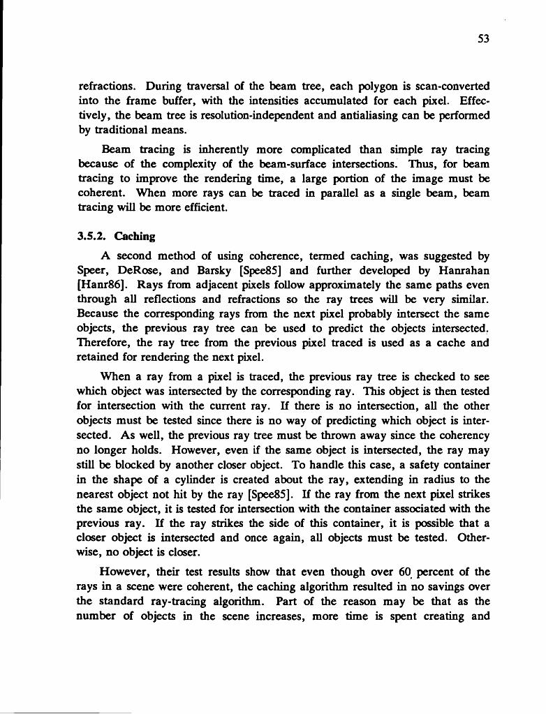
53

refractions. During traversal of the beam tree, each polygon is scan-converted into the frame buffer, with the intensities accumulated for each pixel. Effec­tively, the beam tree is resolution-independent and antialiasing can be performed by traditional means.

Beam tracing is inherently more complicated than simple ray tracing because of the complexity of the beam-surface intersections. Thus, for beam tracing to improve the rendering time, a large portion of the image must be coherent. When more rays can be traced in parallel as a single beam, beam tracing will be more efficient.

3.5.2. CachingA second method of using coherence, termed caching, was suggested by

Speer, DeRose, and Barsky [Spee85] and further developed by Hanrahan [Hanr86]. Rays from adjacent pixels follow approximately the same paths even through all reflections and refractions so the ray trees will be very similar. Because the corresponding rays from the next pixel probably intersect the same objects, the previous ray tree can be used to predict the objects intersected. Therefore, the ray tree from the previous pixel traced is used as a cache and retained for rendering the next pixel.

When a ray from a pixel is traced, the previous ray tree is checked to see which object was intersected by the corresponding ray. This object is then tested for intersection with the current ray. If there is no intersection, all the other objects must be tested since there is no way of predicting which object is inter­sected. As well, the previous ray tree must be thrown away since the coherency no longer holds. However, even if the same object is intersected, the ray may still be blocked by another closer object. To handle this case, a safety container in the shape of a cylinder is created about the ray, extending in radius to the nearest object not hit by the ray [Spee85]. If the ray from the next pixel strikes the same object, it is tested for intersection with the container associated with the previous ray. If the ray strikes the side of this container, it is possible that a closer object is intersected and once again, all objects must be tested. Other­wise, no object is closer.

However, their test results show that even though over 60 percent of the rays in a scene were coherent, the caching algorithm resulted in no savings over the standard ray-tracing algorithm. Part of the reason may be that as the number of objects in the scene increases, more time is spent creating and

54

checking cylinders that are smaller and more likely to be intersected by the next ray. At times, all objects will be tested for intersection even though the original object predicted by the cache is, indeed, the visible object, thereby wasting con­siderable time.

Hanrahan [Hanr86] extended the idea of caching to avoid this situation by replacing this safety cylinder with a list of all possible objects that could be inter­sected by a ray traveling from the first to the second object. A ray is still tested for intersection with the object predicted by the previous ray tree. However, if it does intersect the predicted object, each object in the blocking list must be tested. Only if the predicted object is not intersected does every object have to be tested for intersection.

To simplify creating the list of blocking objects, objects are chosen to be spheres. Alternatively, objects could be bound by spheres. The list of poten­tially blocking objects that lie between two spheres is generated by creating a cone from the originating sphere to the one intersected. Any sphere intersecting this cone could potentially block a ray from the first sphere to the second and is added to the list.

By carefully selecting the order in which pixels are traced, the coherence present in the scene can be better utilized. Rather than tracing pixels in scan line order as is done traditionally, ray tracing is performed so that the complete ray tree is created breadth first. This computes coherent regions completely before moving on to the next.

In general, these methods of using coherence have not been very successful and consequently, are not widely used.

Object coherence is used successfully in the light buffer method [Hain86] for reducing shadow-testing times by noting that an object blocking a light source from one pixel is likely to block the same light for an adjacent pixel. In this way, the object blocking the light from reaching the visible surface is saved and updated each time the light is tested to determine if it casts a shadow on the visi­ble surface. Before other objects from the light buffer list are accessed and tested for intersection, the blocking object is tested. Because it is only important if the shadow ray is blocked before it reaches the light source, not the identity of the closest object, this caching method is much simpler than those for utilizing coherence in tracing all other types of rays.

55

3.5.3. Cone TracingCone tracing [Aman84] assumes coherence since cones instead of rays are

traced. If many rays through the same pixel and from each surface did not fol­low approximately the same paths, they could not be grouped into a cone and traced as a unit. Since a number of rays must be sent through a pixel to per­form antialiasing, they can be traced as a single cone, rather than as separate rays. Such cones are similar to the beams that are generated by Heckbert and Hanrahan [Heck84]. Unlike beam tracing, which identifies the exact portions of a surface that are intersected, only a list is kept of all such surfaces. By includ­ing the fractional amount of the surface intersected, antialiasing can easily be performed. A complete description of the cone tracing algorithm with emphasis on antialiasing can be found in Section 2.4.3.

3.5.4. Parametric SurfacesA form of ray coherence has also been used to ray-trace parametric surface

patches [Joy86]. An iterative method for root finding is used to solve for the ray-surface intersection point. By using the solution for the intersection point from the previous pixel as the initial seed for the current pixel, fewer iterations are needed. In fact, for 90 percent of the rays traced, the algorithm converges in two iterations or less.

A similar form of coherence was used by Blinn to determine an initial seed for a scanline algorithm that displayed parametric surfaces [Lane80]. In this algorithm, the (w,v) pair calculated from the iterations for the previous scan line was used as the initial seed for the current scan line.

3.6. Path TracingPath tracing uses standard Monte Carlo techniques to accelerate the ray­

tracing algorithm by following only one ray from each intersection point [Kaji86]. Instead of following both a reflected and a refracted ray, a decision is made to trace one or the other, resulting in a path through what would have been the ray tree.

For each intersection, a choice is made probabilistically as to whether the reflected or refracted ray is followed. With this method, it is important that the correct proportion of reflection and refraction rays be maintained. Therefore, the number of each type of rays followed is saved. At each stage, the

56

probability of following a type of ray is updated so that the sample distribution will continue to match the desired distribution.

This technique can also be used with distributed ray tracing. Paths, rather than trees, are generated at each surface intersection. Each ray that is traced from a point will be distributed about the appropriate direction.

Processing time is reduced because large portions of the ray tree along with the associated ray-object intersections are eliminated. Since a primary ray con­tributes the most intensity to the pixel, little image quality is lost by tracing only some of the reflected and refracted secondary rays.

Additional phenomena produced by the path tracing algorithm are discussed in Section 2.4.5.

3.7. Visible-Surface PreprocessAnother method of reducing the expense of ray tracing creates, as a prepro­

cess, a visible-surface list for rays traced from each pixel [Wegh84]. Instead of tracing primary rays by testing each object for intersection, this list is used to quickly determine the object intersected. After these first ray-object intersec­tions, ray tracing proceeds as usual.

Such a list of visible surfaces is created as a preprocess and is known as an item buffer and is similar to a z-buffer. The z-buffer is an image space visible- surface algorithm that depth-sorts primitives covering each pixel to determine the visible object. Only the nearest primitive is stored in the z-buffer and frame buffer.

An item buffer is similar, but rather than storing only the visible object, each entry contains a list of all objects projecting onto the pixel. A perspective transformation of the scene performs a two-dimensional projection of all objects onto the virtual screen. From this information, a list of all objects that partially or completely cover a pixel is created. Any ray from the viewpoint passing through the pixel must intersect an object in the list associated with this pixel. Thus, only these objects need be tested for intersection instead of all objects in the scene.

In fact, the item buffer is almost identical to the A-buffer [Carp84], used to implement a scanline hidden-surface algorithm with antialiasing. Each entry in the A-buffer contains a list of objects and fractional coverage information for all objects crossing the pixel.

57

When ray tracing is performed with the visible-surface preprocess, primary rays are treated differently from secondary rays. For each primary ray, the item buffer is accessed and only the objects in the list for that pixel are tested for intersection. However, secondary rays must be traced since their directions can­not be predicted before ray tracing begins and intersection points are calculated.

The creation of the item buffer is not very time consuming and its use can reduce the time required to ray-trace the scene. In realistic environments where many surfaces are diffuse, the average ray tree depth is usually not much more than one. By reducing the time required to trace primary rays, a significant por­tion of the total rendering time can therefore be eliminated. As well, the item list can be used for antialiasing purposes if pixel coverage information is included.

This preprocess simply performs a bucket sort of all objects in the scene at each pixel. Therefore, other scanline algorithms, like Watkins’ algorithm [Suth74], could be used in place of the z-buffer algorithm to achieve the same result. Watkins’ algorithm uses scanline coherence to dynamically create lists of objects crossing each pixel without explicitly creating the depth buffer. A careful implementation of this scanline algorithm requires less time than the version of the visible-surface preprocess suggested.

3.8. Chapter SummaryWhile ray tracing produces impressive images, it is very computationally

expensive because each ray generated must be tested for intersection with each object in the scene to determine the visible surface. Also, to include many of the important features developed, additional rays must often be traced. Because of the computational expense, many attempts have been made to reduce ray tracing times.

Bounding volumes placed around primitives with complicated intersection tests are used to reduce the time for an intersection test. Only when a ray inter­sects the bounding volume is the complex object tested for intersection. Also, scene structuring methods attempt to reduce the number of objects that must be tested for intersection with each ray. Object hierarchies use a hierarchy of bounding volumes to describe the scene. Volume subdivision divides object space either uniformly or adaptively.

58

Tree-depth control, performed either statically or adaptively, is used to reduce the number of secondary rays traced by limiting the depth of the ray tree. Methods to reduce the time for shadow testing have also been suggested in which some shadow rays are never generated or a light buffer describing a subset of objects visible from the light source is created.

Some attempts have been made to use coherence in the ray tracing algo­rithm by noting that rays from adjacent pixels follow approximately the same paths through the scene. Coherent algorithms take the form of tracing cones or beams of light, as well as using information cached from the tracing of the previ­ous pixel. However, such attempts at utilizing coherence have generally not been successful and are consequently, not widely used.

Path tracing uses Monte Carlo techniques to trace only one ray, either the reflected ray or the refracted ray, from each intersection. Also, a visible-surface preprocess has been suggested for determining visible surfaces for primary rays.

Finally, a variety of parallel architectures have been suggested for accelerat­ing the ray-tracing process. One such architecture is vectorization, in which identical calculations are performed in parallel as a single operation. A second uses pipelining to achieve the parallelism, while a third applies multiple proces­sors, each performing parts of the ray-tracing algorithm.

The application of parallel architectures to ray tracing is discussed in the next chapter.

Chapter 4

Parallel Architectures for Ray Tracing

Various hardware architectures that introduce parallelism into the ray­tracing algorithm in order to accelerate the computations have been proposed. By allowing portions of the algorithm to proceed concurrently, the time required for ray-tracing a scene is reduced. The amount that actually executes simultane­ously can range in size from a single instruction to large sections of code. In this way, approaches to reducing ray tracing times have not been limited to the development of software algorithms, but also include algorithms implemented in hardware.

The parallel architectures which have been proposed are very diverse. Some require the construction of special-purpose hardware while others can utilize existing systems. Vector machines that perform an operation on all elements of a vector simultaneously can be used to intersect many rays with the same object at the same time [Plun85]. Different forms of pipelining have also been sug­gested [Ulln83, Nish83]. Pipelining involves dividing the algorithm into stages that operate concurrently, but on different data items. Multiprocessor systems have also been proposed in which processors are assigned either to regions of image space [Dube85, Degu84] or to regions of object space [Ulln83, Clea86, Dipp84, Nemo86].

4.1. Parallel Architectures in Computer GraphicsParallel architectures have previously been used in other areas of computer

graphics, specifically in traditional rendering systems for raster graphics. Paral­lelism has been exploited in the higher-level operations of transformations, clip­ping, projection and coordinate mappings as well as in low level scan conversion of primitives involving visible-surface calculations, shading and antialiasing.

The “geometry engine” [Clar82] has been designed to implement the graph­ics pipeline, a series of transformations which must be applied to each object in the scene. This pipeline is composed of modeling transformations, clipping to

59

60

the viewing volume, perspective and orthographic projections, window-to- viewport mapping, and scaling to device coordinates. Twelve of the geometry engines are assigned to implement the stages in this pipeline. The first four pro­cessors handle transformations involving matrix multiplications, with the results passed to the clipping stage of the pipeline, where each of the six processors clips objects against a different clipping plane. Clipped objects are then passed to the last two processors which project them onto the viewport by scaling them to dev­ice coordinates. Objects defined in world coordinates are passed into the pipe­line and primitives suitable for scan conversion are returned at the end.

Other architectures operate at the lower end of the graphics pipeline, where primitives are scan-converted into the frame buffer and displayed. One such architecture performs hidden-surface removal and antialiasing for polygons by assigning a processor to each polygon [Wein81]. All processors scan-convert their assigned polygons in parallel and pass the results directly to their compara­tor processors, which are organized in a pipeline. These comparator processors maintain a depth-sorted list of all polygons that are potentially visible at each pixel. To facilitate antialiasing, this list is passed through a pipeline of proces­sors which filter the results to calculate the final intensity.

Pixel-Planes [Fuch81] places extra hardware at each pixel of image memory to simultaneously determine the pixels covered by a polygon and to perform hidden-surface removal and smooth shading. Each pixel in the frame buffer is augmented by a pair of one-bit adders, with an extra bit of storage. The one-bit adders are organized in a tree, with each evaluating in parallel the expression F (x ,y ) = Ax + By + C , where x and y are pixel positions. Processors use the results from parent processors in the tree and pass their results on to other processors. By expressing edges of polygons, equations for z values of the polygon plane and red, green and blue intensity values as planar equations, pro­cessors can determine the pixels in the polygon, perform depth-buffering and do smooth shading. An extension to Pixel-Planes produces shadows and performs fast shading of spheres [Fuch85]. As well, Pixel-Powers [Gold86] evaluates qua­dratic expressions of the form F (x ,y ) = Ax 2 + Bxy + Cy 2 + Dx + Ey + F to render quadratic objects such as convex polyhedra and cylinders.

Another system utilizes a polygon buffer to perform hidden-surface elimina­tion and antialiasing [Fuss82]. The frame buffer is actually a collection of pro­cessors, each of which is assigned a triangle. The processors scan-convert the triangles, calculating the intensity and depth value for each pixel. This

61

information is passed on to a binary tree of comparators which perform hidden- surface elimination and antialiasing for each pixel.

Fiume and Fournier suggest using an ultracomputer, a system with parallel processing units and a shared memory, to perform parallel scan conversion with hidden-surface elimination and antialiasing [Fium83]. In the ultracomputer, a multi-stage network connecting the processors to shared memory can combine operations destined for the same variable into a single operation before passing it onto the next stage in the net. To implement a depth-buffer algorithm, an instruction, replace .minimum, is proposed which assigns to a variable a value associated with the lower of two values. Essentially, this is the major operation performed in depth-buffering. Hidden-surface elimination is performed one scan line at a time and antialiasing is done with subpixel coverage information.

Ullner designed two architectures for hidden surface and line elimination [Ulln83]. The first organizes processors in a binary tree, with leaf processors scan-converting polygonal surfaces to produce spans on a scanline. These spans are passed to parent processors where they are combined into a single non­overlapping span, with this continuing until the root processor is reached. The second architecture performs hidden-line removal for line drawings by organizing processors, each of which is assigned a polygon, into a pipeline. Edges of all polygons are passed into the pipeline, where they are clipped to the polygon at each stage. After all edges have passed through the pipeline, all hidden lines will have been removed.

An architecture for real-time animation including hidden surfaces and sha­dows has also been designed [Whel86]. A two-dimensional array of processors is assigned to regions of image space. Visible surfaces for these regions are deter­mined simultaneously by projecting an object-space region onto the subscreen. A parallel shadow algorithm, using information from the local processor and from other processors is then performed.

Recently, a multiprocessor graphics system consisting of many identically- programmed processors operating in parallel has been designed [Torb87]. The system implements all aspects of a graphics rendering package, with graphics commands being distributed to the first available processor. Processors perform transformations, clipping, hidden-surface removal, and shading for primitives which include curves and surfaces. Representations of two-dimensional primi­tives for which all the operations have been performed are given to image memory, where they are scan-converted.

62

4.2. Parallelism and Ray TracingCertain aspects of the ray-tracing algorithm make it suitable for paralleliza­

tion, the most important of which is the lack of effective coherence. Although ray tracing does exhibit some form of coherence in that rays through a pixel fol­low approximately the same path as the rays through nearby pixels, striking most of the same objects and generating secondary rays in similar directions, it is not clear that this coherence can be easily used.

In the ray-tracing algorithm, the shading of one pixel is treated as a com­pletely separate problem from the shading of another pixel. Ray tracing is per­formed for the pixels one at a time, using no information obtained during the shading of other pixels. Hence, all rays generated from different pixels are com­pletely independent.

Although the results for one pixel are entirely independent of the next, the actual steps required to shade the pixels are the same. A primary ray is gen­erated through the pixel and the visible surface is determined by intersecting all of the objects. The diffuse and ambient components are calculated and a sha­dow ray is sent to each light source to see if the intersection is in shadow. If the surface has reflective or transparent qualities, rays are generated in these direc­tions and the process is repeated recursively. Consequently, there are many independent actions that are the same, although they operate on different data.

While lack of coherence has restricted the standard ray-tracing algorithm, it is just this lack of coherence that admits the use of parallel architectures. By re-organizing the order of computations for ray tracing, parallelism can be better utilized. The architectures that have been proposed for ray tracing reorder the steps of the ray-tracing algorithm in various ways.

In the following sections, the various parallel architectures which have been applied to the ray-tracing problem are examined. In addition to describing the features of each system, other aspects of the parallelization will be discussed. First, although many such architectures have been proposed, few have been implemented. As well, most architectures perform only very simple ray-tracing algorithms, although many of the features and acceleration techniques intro­duced for uniprocessor ray tracing and described in Chapters 2 and 3 are impor­tant. Some of these methods are deemed essential for ray tracing realistic scenes. For many of these hardware architectures, some techniques will be diffi­cult to implement because of the way in which parallelism is introduced.

63

Any architecture should be able to render a scene modeled with multiple primitive types, including those with iterative solutions and fractal surfaces. As well, any of these primitives should be able to be texture mapped. Antialiasing, with either uniform sampling or preferably stochastic sampling, is essential for producing images with minimal sampling artifacts. Finally, distributed ray trac­ing, which can add many blurred effects to an image, is very important. Some applications may require only a subset of these features in which case fewer res­trictions would apply to the architecture.

Many of the acceleration techniques proposed for uniprocessor ray tracing such as bounding volumes to reduce the number of complicated intersection tests and data structures to describe the scene are routinely implemented in most ray­tracing programs. Tree-depth control, both fixed and adaptive, should always be used. As well, methods of reducing shadow testing times, including only tracing rays that are promising and using a light buffer to cull objects, are important for a uniprocessor system. If the parallelism employed by an architectures precludes the use of these standard acceleration techniques, the advantages of using the architecture may be negated.

4.3. VectorizationA vector machine that employs parallelism by operating on many data ele­

ments in parallel has been utilized to reduce the ray-object intersection time in ray tracing [Plun85]. A number of rays are queued and then intersected with an object in a single calculation, producing an intersection value for each ray. The process is repeated for each object in the scene and the closest intersection saved for each ray.

With vectorization [Hama84, Hwan84], execution time is reduced because a vector processor performs the same operation simultaneously on all elements of an array. However, to be vectorized, the computation must meet certain con­straints. First, the operation must be applied to every element in the vector. Secondly, the calculation must not depend upon other elements in the same vec­tor. A vector operation can involve constants, variables and other vectors, as long as the two constraints are met. An example is shown below:

FOR ( i = 1 t o n)a [ i ] «- a [ i ] + c * b [ i]

END

64

This calculation can be vectorized because it performs the same operation on each element of a and does not use other elements in the vector in the same cal­culation. The resulting vectorized instruction is:

a [ l : n ] «- a [ l : n ] + c * b [ l : n ]

Ray tracing is suitable for vectorization for two reasons. The first is that the same procedure can be performed for all rays that are generated, regardless of whether they are primary or secondary. In the standard ray-tracing algorithm, each ray is tested for intersection with every object in the scene and the closest point of intersection returned. Thus, the same basic computations are applied to every ray regardless of where the ray originated.

The second reason that a vector machine can perform ray tracing is that most rays are independent, so that computations involved in tracing one ray need not depend in any way upon those involved in tracing another. This is cer­tainly true for all primary and secondary rays that originate from different pix­els. Pixels are always traced separately and no results from one are used to gen­erate rays from another. Even rays from the same pixel, although they may depend on a previous ray-surface intersection to exist, are independent.

Hence, the algorithm can be rearranged so that many different rays are intersected with an object simultaneously, one object at a time. In the vector­ized algorithm, any generated ray that needs a visible surface determined is placed in a queue. A single vector instruction intersects all rays with a single object, producing another vector of intersection points.

To begin the vectorized algorithm, enough primary rays are generated to fill the queue. Next, these rays are intersected with the first object in a vector cal­culation and the resulting intersection points are saved. This process is repeated for each object in the scene until all have been intersected. The nearest intersec­tion point for each ray is saved after each vectorized intersection. For each ray that intersects an object, shadow, reflected and refracted rays are generated and fed back into the ray queue. Thus, after the initial primary rays are created, the queue contains a mixture of primary and secondary rays. Once the queue is filled, the intersection process is repeated. When ray tracing is completed for a pixel, the intensity can be calculated.

65

The vectorized ray-tracing algorithm is outlined below:

while (more pixels to shade){

1. Add more rays to the queue until it is filled.2. Calculate the intersections of all rays in queue

with each object in the scene, one object at a time.3. Determine closest object intersected for each ray.4. For all rays that strike a visible surface, spawn

more rays representing reflections and refractions, and shadow rays for shadows.

5. Calculate intensity of pixels whose ray-tracing process is complete.

Vectorized ray tracing has been implemented on a CDC CYBER 205 super­computer, consisting of a vector processor and a scalar processor [Plun85]. Although the algorithm implemented performs ray tracing for a Constructive Solid Geometry system used to model mechanical parts, it is easily generalized to standard ray tracing. In this system, spheres, cylinders, cones and paral­lelepipeds are just some primitive objects that have been defined. As well, spe­cial purpose vectorized routines for traversing the CSG tree are available.

While there is little doubt that vectorization greatly reduces the total time for intersection calculations compared to the same algorithm implemented on a uniprocessor, additional factors must be considered. First of all, a significant amount of overhead in time and storage is involved in managing the queues of rays and results. Since rays are no longer traced in pixel order, the algorithm must keep track of which rays belong to which pixel, which pixels are active, and which pixels have completed the ray-tracing portion of the algorithm.

As well, additional time must be spent in calculating the final intensity for each pixel. Each ray-object intersection identifies a visible surface for which intensity values must be calculated and accumulated for the pixel. However, the diffuse component for a surface cannot be calculated until the shadow rays have been processed. Therefore, any information pertaining to the diffuse contribu­tion must be saved until the shadow rays have been processed, creating extra overhead for the scalar processor.

66

Memory requirements can be a problem for the vectorized algorithm. Suffi­cient storage must be available for the two queues containing rays and intersec­tion results. If R rays are intersected in parallel during one vector calculation and the closest intersections retained at each iteration, enough storage is needed for 4/? numbers. These numbers represent t, the intersection’s distance along the ray, and the identifier of the intersected object. One pair describes the current intersection and one describes the closest intersection found thus far. This is not a significant amount of storage. However, in CSG applications for which the system was designed, the amount of storage required would be 4NR numbers, where N is the number of objects in the scene. All intersection results must be saved because the primitive with the nearest intersection is not necessarily the visible surface.

Unfortunately, there is a tradeoff between the amount of storage required and the computation time. In a vector machine, the computation time for a vec­tor operation consists of two components: a constant start-up time and a process­ing time dependent on the number of elements in the vector. Thus, the vector processor is used most efficiently if the vector is made as large as possible, thereby increasing the amount of storage required for the intersection results. Hence, the efficiency of the intersection operations cannot be improved without increasing the storage requirement.

One feature of vectorized ray tracing is that multiple primitives can be used to model the scene because the rays are intersected with a single object at a time. However, primitives such as parametric surfaces which have iterative intersection tests are difficult to vectorize because solutions for some rays con­verge faster than others. To handle this type of primitive, an equal number of iterations would have to be performed for each ray, regardless of the number required for convergence. This will require unnecessary work for some rays. As well, an incorrect result may be returned for other rays because too few itera­tions were performed. Alternatively, iterations could be performed until solu­tions for all ray-object intersections had converged. However, this requires extra overhead to determine for which rays solutions have not yet been found.

Fractal surfaces present a problem because in the vectorized algorithm, a ray must be intersected with every primitive in the scene. Unfortunately, if a fractal surface is fully instantiated before ray tracing begins, millions of polygons may be generated. To intersect every ray with all polygons is not practical and is especially wasteful if most rays do not strike any part of the fractal surface.

67

To attempt to modify the vectorization so that a hierarchy can be used may be very difficult as the fractal surface would have to be treated much differently from all other primitives. Thus, fractals are not easily included in ray tracing that is vectorized in this manner.

Primitives which are used to model the scene can be texture-mapped, with such maps stored in the scalar processor where the intensity calculations are per­formed. To perform antialiasing, both uniform sampling and stochastic sampling can be used. Distributed ray tracing, requiring uncorrelated sampling of each phenomenon being modeled, can be performed because all rays are generated by the scalar processor. However, using different tables to describe which portion of a function a ray should sample becomes complicated because rays from more than one pixel are now allowed to be active at the same time. In the uniproces­sor solution, the table of random permutations is recreated for rays traced from each new pixel. To avoid creating and saving a table for each active pixel, a single permutation table can be used by all rays if the index for the correct per­mutation is now a function of the ray tree node number, phenomenon being modeled, and pixel identifier. Selection of an entry is still based on the number of the grid square through which the corresponding primary ray passes.

In order to vectorize the ray-tracing calculation, the algorithm relies on the simplicity of intersecting many rays with a single object simultaneously. There­fore, no form of scene structuring which would normally cull many objects from being tested for intersection with a ray is implemented. Thus, rays are tested for intersection with every object in the scene to determine the closest intersection point. Because no form of scene structuring is used, a tradeoff exists. More intersection tests in total are performed by the vectorized algorithm than by an optimized uniprocessor algorithm utilizing scene structuring. If the vector machine can perform all intersection tests in less time than the smaller number on a uniprocessor, culling may not be as critical as in other architectures.

To utilize scene-structuring methods, a matching between subsets of objects and rays that must be tested for intersection must be found. With any form of scene structuring, additional overhead will be introduced to record how the rays are traversing the parts of the data structure. Also, the number of rays in the vector will be decreasing at each step of traversal. Therefore, at some point, it will not be advantageous to cull rays or objects. With modifications, some struc­turing technique could be implemented, but it is not clear whether structuring is will have any effect.

68

Bounding volumes also may not be practical since the test would simply cull many of the rays from having to be tested for intersection with an object. Once again, this reduces the size of the vector, possibly having little effect on the intersection time. However, for objects such as fractal surfaces or primitives with complicated intersection tests, testing the queue of rays against the bound­ing volume may be useful. Since it is likely that at least one ray in the queue will intersect the bounding volume, time to test the object against at least one ray will be necessary.

Before any type of scene structuring method or bounding volumes can be used, these tradeoffs must be more closely examined. While such methods would reduce the total number of ray-object intersection tests, this would not make full use of the capabilities of the vector processor.

Tree-depth control, both fixed and adaptive, can be used to reduce the number of rays traced. Similarly, the number of shadow rays traced can be lim­ited by passing only those that point towards light sources contributing a signifi­cant diffuse intensity to the vector processor. However, using light buffers created for each light source to identify a small list of objects to be tested for intersection with a shadow ray is possible only if shadow testing is done com­pletely by the scalar processor. Currently, shadow rays are generated and passed to the vector processor where they are intersected with each object in the environment. Because a subset of objects cannot be selected, testing will con­tinue until every object has been intersected even though testing for shadow rays can terminate when the first object blocking the ray is found.

If multiple frames are being ray-traced, additional constraints result. When only the camera position changes between frames, pixels from different frames can be traced simultaneously. However, if objects move between frames, pixels from different frames would have to be tested for intersection with objects that may be in different positions. Since such intersections cannot be performed in a single vectorized calculation, the tracing of a new frame cannot be started until the previous one has been completed.

Motion blur, a phenomenon produced by distributed ray tracing, presents additional problems because positions of the objects are now different for rays traced at different instants of time during a single frame. Since groups of rays are tested with each object in parallel and the object position is different for each ray, the calculation is not easily vectorized. Groups of rays traced at exactly the same instant of time would have to be queued and then tested with each object

69

moved to the correct location. This will be difficult, if not impossible to do, and requires calculating new object positions for each group of rays.

A final consideration is the utilization of the two processors of the super­computer. The vector computer is used only to implement the vectorized ray- object intersection calculations, leaving the scalar processor responsible for all other aspects of the algorithm. These include processing intersection results, generating new rays, and shading the pixels. Because ray-object intersection results are returned to the scalar processor in large groups at random intervals, the processor may be idle while the vectorized intersections are carried out, and later heavily loaded as it tries to process results for all rays. For larger groups of rays, this is more likely to happen. As well, the vector processor cannot begin additional intersection calculations until the scalar processor has generated enough rays to fill the queue. Although this may leave the vector processor idle a great deal of the time, this processor can carry out intersection calculations fast enough that the scalar processor is not often idle. Therefore, the number of rays in the queue must be adjusted to achieve the proper balance.

So, while vector calculations are very fast, much of the work performed is unnecessary. Some of what has been gained by being able to test many objects for intersection in parallel may be lost by the very fact that many objects can be culled in a uniprocessor ray-tracing algorithm. Because significant overhead is generated, the bottleneck in the algorithm, which was previously the intersection testing, may move into the scalar processor. All tradeoffs must be carefully con­sidered before attempting to alter the vectorized algorithm by including scene­structuring or bounding-volume techniques.

4.4. PipeliningPipelining [Hama84, Hwan84] is another method of accelerating the ray­

tracing computations. In a pipelined system, a procedure that must be applied to many data items is first decomposed into subtasks or stages, each of which can be performed by a separate processor or by separate circuitry. The stages are ordered so that the output of one stage becomes the input to the next. Data is streamed through this pipeline in an assembly-line fashion so that at the output end of the pipeline, all the required operations have been performed on each data item, completing the intended procedure.

70

If a procedure has been divided into N subtasks, each of these subtasks will execute concurrently on different data. When the pipeline is full, the N stages are able to process N data items simultaneously, thus reducing the total process­ing time. This parallelism is possible only because the operations performed on one data item are independent of those performed on any other. While a data item is being operated on by one stage, other data items can be operated on by other stages, resulting in a great deal of concurrency. For a longer pipeline with many stages, more data items can be processed in parallel.

The specific task assigned at each stage can vary from being a single arith­metic operation, such as an addition, to many operations forming a long algo­rithm. In both cases, each stage works in parallel with the others.

A simple example of pipelining exists in the fetch-execute cycle, in which the two operations are overlapped. Instead of fetching an instruction, executing it, and fetching the next instruction, the next instruction is prefetched by the pro­cessor during execution of the current instruction. Since the two operations are usually not dependent, they can be overlapped, eliminating wait time while the next instruction is fetched.

In any pipelined system, it is important that the stages be selected so that they require approximately the same amount of time to complete. Otherwise, bottlenecks will develop at stages that need considerably longer to complete than the others. The other stages would have to wait with their output to the slower stage or wait for input from a slower stage. This holds up the entire pipeline. In fact, the pipeline processing rate is exactly that of the slowest stage.

There are some aspects of the ray-tracing algorithm that make it suitable for pipelining. Various pipelined architectures that use special purpose processors and circuitry have been proposed. Two architectures that employ pipelining for ray-object intersections have been suggested [Ulln83]. One is a ray-tracing peri­pheral that has a separate intersection processor with pipelined circuitry and the other is a pipeline of processors each of which intersects rays with an object. As well, a multiprocessor ray casting system that utilizes pipelining has been imple­mented [Nish83]. Each of these proposals will be discussed in detail.

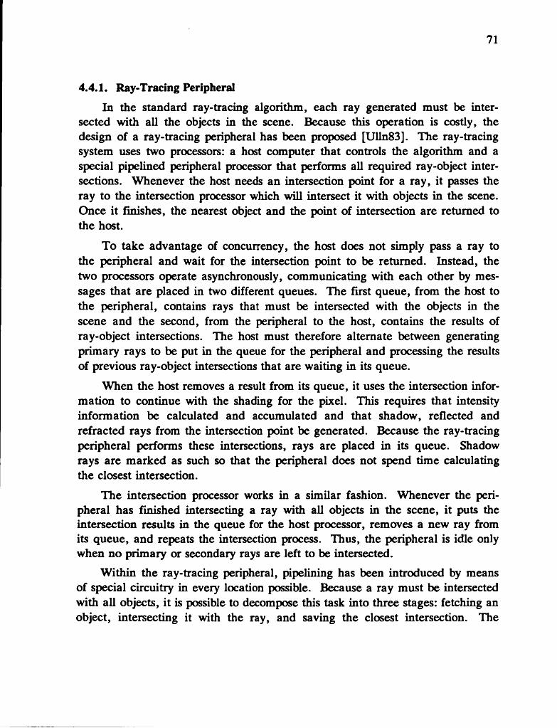
71

4.4.1. Ray-Tracing PeripheralIn the standard ray-tracing algorithm, each ray generated must be inter­

sected with all the objects in the scene. Because this operation is costly, the design of a ray-tracing peripheral has been proposed [Ulln83]. The ray-tracing system uses two processors: a host computer that controls the algorithm and a special pipelined peripheral processor that performs all required ray-object inter­sections. Whenever the host needs an intersection point for a ray, it passes the ray to the intersection processor which will intersect it with objects in the scene. Once it finishes, the nearest object and the point of intersection are returned to the host.

To take advantage of concurrency, the host does not simply pass a ray to the peripheral and wait for the intersection point to be returned. Instead, the two processors operate asynchronously, communicating with each other by mes­sages that are placed in two different queues. The first queue, from the host to the peripheral, contains rays that must be intersected with the objects in the scene and the second, from the peripheral to the host, contains the results of ray-object intersections. The host must therefore alternate between generating primary rays to be put in the queue for the peripheral and processing the results of previous ray-object intersections that are waiting in its queue.

When the host removes a result from its queue, it uses the intersection infor­mation to continue with the shading for the pixel. This requires that intensity information be calculated and accumulated and that shadow, reflected and refracted rays from the intersection point be generated. Because the ray-tracing peripheral performs these intersections, rays are placed in its queue. Shadow rays are marked as such so that the peripheral does not spend time calculating the closest intersection.

The intersection processor works in a similar fashion. Whenever the peri­pheral has finished intersecting a ray with all objects in the scene, it puts the intersection results in the queue for the host processor, removes a new ray from its queue, and repeats the intersection process. Thus, the peripheral is idle only when no primary or secondary rays are left to be intersected.

Within the ray-tracing peripheral, pipelining has been introduced by means of special circuitry in every location possible. Because a ray must be intersected with all objects, it is possible to decompose this task into three stages: fetching an object, intersecting it with the ray, and saving the closest intersection. The

72

execution of each of these stages can be overlapped. The first stage fetches the next primitive from storage and passes it to the second stage which performs the intersection calculation. The third stage is given the task of checking the inter­sections coming out of the second stage and saving the closest one. After the last object has been intersected with the ray, the saved values, representing the closest object and intersection point, are returned to the host. Each object in the scene is streamed past the stored ray in turn to fill this pipeline.

The most costly operation in the pipeline is that of intersecting the ray with an object. In comparison, the operations of fetching an object and saving the closest intersection are trivial. By allowing only one primitive type, the polygon, this intersection calculation can also be pipelined to avoid a bottleneck. The intersection procedure is divided into three subtasks. The first calculates the parameter, t, which is the distance along the ray of the intersection point. The second calculates the exact point of intersection with the plane of the polygon. The third calculates two parameters, u and v, which represent the point of inter­section with respect to the polygon. The calculation of t is also pipelined inter­nally with four stages. With the selection of only one primitive type, the speed of the intersection stage is predictable and by choosing a simple primitive, such as the polygon, the intersection stage will require approximately the same time as the other stages.

The extensive amount of pipelining within the ray-tracing peripheral increases the amount of concurrency that can be attained. Not only can the host and peripheral proceed in parallel, but parts of the expensive ray-object intersec­tion tests can execute concurrently. Parallelism and pipelining within the peri­pheral are implemented with custom chips.

To avoid intersecting each ray with every polygon in the scene, an addi­tional processor is used to determine which objects are in the ray’s path. Volume subdivision is used to uniformly divide the scene volume into rectangu­lar parallelepipeds so that only the objects in the volumes that the ray enters are input to the pipeline to be intersected with the ray. These volumes are checked one at a time so that if no intersection is found in the first subvolume, only then are the objects in the next subvolume passed in for intersection. Unfortunately, this solution adds extra calculations in the ray-tracing peripheral and implies additional synchronization between the peripheral and this processor.

73

The system, as described by Ullner, is limited to four-sided polygons, which severely restricts its flexibility. However, this not a restriction of the pipelining between the two processors, only of the internal intersection pipelining. Multiple primitive types and primitives with iterative intersection calculations present a problem for the system. A primitive that has an iterative solution could be used to model scenes, but the intersection stage of the pipeline will be very long, slow­ing down the entire pipeline. To allow multiple primitives, either pipelined cir­cuitry would have to be added for every new intersection test or all internal pipe­lining would need to be removed. The disadvantages of pipelining every inter­section calculation outweigh the advantages. First, it may become difficult and expensive to design the chips; and, because the calculations are pipelined in hardware, the system is not easily extended to intersect new and different primi­tives. If all pipelining was removed, the intersection stage would be too long and the length would vary with the complexity of the intersection test. By using bounding volumes about primitives, the ray-bounding volume intersection test would be simple and could be pipelined internally. Only if the ray intersected the bounding volume would the ray be intersected with the complicated object. At this point, the intersection stage would be the bottleneck in the pipeline. However, with bounding volumes, the variation in length would be minimized.

Fractal surfaces will be more difficult to implement with the peripheral. Of course, the surface can always be fully instantiated before ray tracing begins, generating many polygons. If Kajiya’s bounding-volume hierarchy is to be used, the intermediate processor would need to generate and enclose the fractal sur­face, passing the appropriate bounding volumes or facets to the intersection pro­cessor to be intersected with the ray. As well, the peripheral could not save the closest intersection for this primitive, but would return each result to the inter­mediate processor which would decide which other bounding volumes or facets to pass to the peripheral. This means that a fractal surface would have to be treated differently from other primitives. Alternatively, the peripheral could test rays for intersection only with the root cheesecake of the fractal surface. If this was the closest intersection, the host could then generate the surface and find the exact facet and point of intersection. Of course, this would completely bypass the pipelining abilities of the system.

Texture mapping of all primitives is possible since the maps can reside in the host where the intensity calculations are performed. Either form of antialiasing through uniform supersampling or stochastic sampling can also be performed in

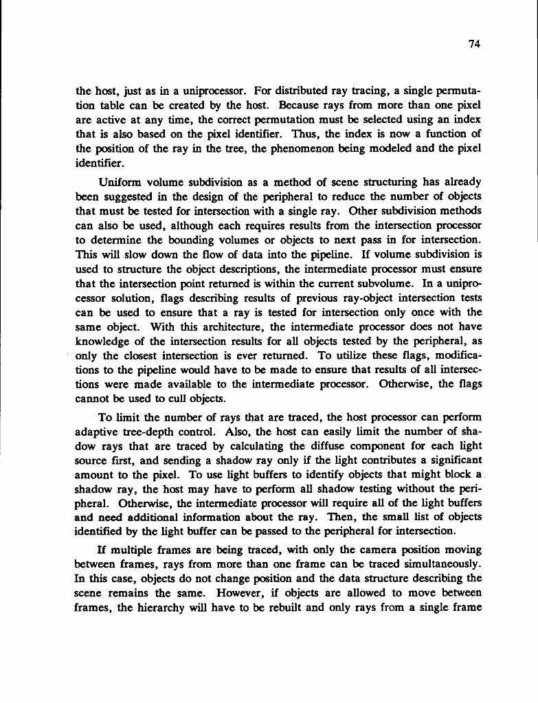
74

the host, just as in a uniprocessor. For distributed ray tracing, a single permuta­tion table can be created by the host. Because rays from more than one pixel are active at any time, the correct permutation must be selected using an index that is also based on the pixel identifier. Thus, the index is now a function of the position of the ray in the tree, the phenomenon being modeled and the pixel identifier.

Uniform volume subdivision as a method of scene structuring has already been suggested in the design of the peripheral to reduce the number of objects that must be tested for intersection with a single ray. Other subdivision methods can also be used, although each requires results from the intersection processor to determine the bounding volumes or objects to next pass in for intersection. This will slow down the flow of data into the pipeline. If volume subdivision is used to structure the object descriptions, the intermediate processor must ensure that the intersection point returned is within the current subvolume. In a unipro­cessor solution, flags describing results of previous ray-object intersection tests can be used to ensure that a ray is tested for intersection only once with the same object. With this architecture, the intermediate processor does not have knowledge of the intersection results for all objects tested by the peripheral, as only the closest intersection is ever returned. To utilize these flags, modifica­tions to the pipeline would have to be made to ensure that results of all intersec­tions were made available to the intermediate processor. Otherwise, the flags cannot be used to cull objects.

To limit the number of rays that are traced, the host processor can perform adaptive tree-depth control. Also, the host can easily limit the number of sha­dow rays that are traced by calculating the diffuse component for each light source first, and sending a shadow ray only if the light contributes a significant amount to the pixel. To use light buffers to identify objects that might block a shadow ray, the host may have to perform all shadow testing without the peri­pheral. Otherwise, the intermediate processor will require all of the light buffers and need additional information about the ray. Then, the small list of objects identified by the light buffer can be passed to the peripheral for intersection.

If multiple frames are being traced, with only the camera position moving between frames, rays from more than one frame can be traced simultaneously. In this case, objects do not change position and the data structure describing the scene remains the same. However, if objects are allowed to move between frames, the hierarchy will have to be rebuilt and only rays from a single frame

75

traced at any time.More complicated object motion results when distributed ray tracing is used

to model motion blur. Then, many rays from the same frame will be traced at different instants of time. Since objects must be moved into their correct posi­tion at the time of the ray before being tested for intersection, problems with this method of parallelism will result. In a uniprocessor system, a primary ray and all its descendants that all occur at the same time will be traced in order, result­ing in fewer changes to the hierarchy and object positions. Because rays in this architecture are not traced in such an order, the hierarchy would have to be rebuilt more frequently. However, by using bounding volumes in time to enclose the objects, objects need only be moved to their correct position if the bounding volume is intersected by the ray. Preferably, a bounding-volume hierarchy is used to describe the scene instead of uniform subdivision, but this is not necessary. Then, this data structure only needs to be recreated for succes­sive frames.

The design and construction of the ray-tracing peripheral may be very costly. A t the same time, because the system is custom-designed for ray tracing, many unnecessary costly mechanisms can be eliminated from the machine while money can be spent on aspects of the architecture that will accelerate the algo­rithm. If the system performs only ray tracing, a very simplified operating sys­tem is needed because all multi-user functions can be eliminated. For example, timesharing, processor scheduling, job scheduling and complicated memory management are all unnecessary in this system. Also, only a subset of the machine instructions is needed and most i/o functions can be eliminated.

4.4.2. Ray-Tracing Pipeline

The ray-tracing pipeline is another parallel architecture that relies heavily on pipelining to decrease computation time [Ulln83]. With this method, a processor is assigned to each object and is responsible for performing intersection tests between this object and the rays. The processors are arranged to form a pipeline in which rays enter at one end and intersection results are returned at the other.

A t each stage of the pipeline, the ray is tested for intersection with its object. To ensure that the nearest object intersected and point of intersection are returned at the other end of the pipeline, information about the nearest intersec­tion found is passed through the pipeline along with the ray. Therefore, each processor must update the closest intersection information after an intersection

76

with the object is found.A host processor controls the ray-tracing procedure. When an intersection

point is required for a ray, the ray is passed into the processor pipeline. At a later time, the host retrieves the intersection results from the other end of the pipeline. This communication is performed with two queues: one is a queue of rays that require intersection calculations and the other is a queue of results from the ray-tracing pipeline.

Acceleration of the ray-tracing algorithm is achieved for two reasons. The first is that the host processor and the pipeline operate in parallel. Although they depend on each other for input, the queues are generally full enough to keep the processors from becoming idle. The second reason is due to the effects of pipelining. Each processor calculates the intersection of a ray and an object. When the pipeline is full, each of N processors is intersecting an object simul­taneously, resulting in N objects in total being intersected in parallel. Less total time is needed to produce the intersections because many are being performed in parallel.

Before ray tracing can begin, the pipeline must be loaded with the primitives that describe the scene. One at a time, the objects are downloaded from the host to the first processor in the pipeline. When a processor receives a new prim­itive, it shifts the previous primitive’s description to the next processor, continu­ing until all primitives have been loaded.

A variety of problems exist with the ray-tracing pipeline. In the proposed design, a processor is required for each object in the scene. Clearly, this is not at all practical because even simple scenes are formed from many primitives. A complex scene can consist of thousands of objects, and one processor per object is not possible. The only solution would be to assign more than one object to each processor, introducing additional problems. If the processors operate on different numbers of primitives, the intersection times for each pipeline stage would vary. When this happens, the entire pipeline is held to the time required by the slowest stage.

Since a pipelined system achieves the greatest concurrency with many stages, it is desirable to increase the number of stages, thereby increasing the number of processors required. However, a very large number of processors is not practical because of cost, difficulty of connections and probability of failures.

77

An additional drawback of the design is that it is really limited to only one type of primitive. If more than one type is allowed, the time required to inter­sect a ray with each primitive type would have to be very similar. Intersection times for different primitives generally vary greatly so processors will require widely different times to perform a ray-primitive intersection, resulting in bottlenecks in the pipeline. For this reason, the proposed pipeline has been lim­ited to ray tracing polygons. For the same reason, primitives requiring iterative solutions present a problem. A processor assigned to this primitive type will take randomly different times to perform the intersection, depending upon the number of iterations needed for each ray. Thus, this stage will generally have a longer, but unpredictable time.

Fractal surfaces cannot be handled by the ray-tracing pipeline. If the sur­face is fully instantiated before ray tracing begins, a processor would be needed for each facet, which clearly is not possible. Another option is to treat the sur­face as a single object which is assigned to one of the processors. In this case, considerable storage would be required for this processor, which would have to create a bounding-volume hierarchy as the surface is evolved. Also, the time to intersect this primitive with a ray will produce a bottleneck in the entire pipeline.

Other features that produce realistic images can easily be incorporated into the system because the host processor is responsible for the generation of all rays and performing the intensity calculations. Thus, all primitives can be texture mapped. Spatial antialiasing by sampling the pixel area with many primary rays is no different from a uniprocessor algorithm. For distributed ray tracing, in which jittering is performed in the other dimensions, the permutation table index will also have to be based on the pixel label because there is no restriction on the number of pixels that are active at a single time.

Unfortunately, some of the most important methods of accelerating the standard ray-tracing algorithm cannot be incorporated into the ray-tracing pipe­line. Bounding volumes are not precluded, although the pipeline will still be as slow as the slowest stage where the bounding volume is intersected and the prim­itive then tested. As well, because a processor is assigned to each object, rays are intersected with every object in the scene, even though most intersection cal­culations are unnecessary. While this is necessary to allow pipelining, scene structuring which greatly accelerates a uniprocessor system cannot be utilized. Unfortunately, with pipelining implemented in this form, it is not possible to select a subset of the objects in the scene to be tested for intersection. Thus,

78

much additional work is performed overall by the architecture in order to achieve the pipelining.

Tree-depth control, to reduce the number of rays traced is done by the host. Also, the host can easily create only those shadow rays aimed at light sources which contribute something to the intensity of the pixel. Light buffers cannot be used because a subset of objects cannot be selected in the pipeline. Then, the only way to utilize this technique is to treat shadow rays differently from all other rays, having the host perform these intersection tests.

If multiple frames are rendered with only the viewpoint changing between frames, pixels from more than one frame can be traced at a time since object coordinates remain the same. However, if objects move between frames, the coordinates in each processor will have to be modified for each frame traced. Therefore, tracing rays from only a single frame at a time avoids the recalcula­tion of object coordinates for each ray. Distributed ray tracing modeling motion blur will require object positions to be altered for each ray passing through the pipeline, as rays from the same primary ray will not be created in order. Thus, a ray will have to carry with it time information, which each processor can use to calculate the position of the assigned object for each ray received by the pro­cessor. However, this will be very costly, because a ray must be tested for inter­section with each object. Also, bounding volumes in time cannot be used to reduce time spent moving objects to the correct position.

4.4.3. Links-1Another form of pipelining was implemented in a multiprocessor-based ray

casting architecture called Links-1 [Nish83]. Pipelining was present in the early version of the system, but was removed when the architecture was extended to trace reflected and refracted rays. In the ray casting system, a number of pipe­lines are set up, each of which is designed to render a group of pixels. For pipe­lining purposes, the image rendering procedure is divided into three stages: object sorting, ray casting, and shading.

The ray casting portion of the architecture was not described in great detail, but the following can be said about each stage. The first stage, object sorting, searches all objects to find those likely intersected by the ray, possibly with bounding-volume tests, and orders these from near to far. The second stage, ray casting, determines precise intersection points, calculates the intersection dis­tance, t, along the ray and selects the closest object. The third stage, shading,

79

determines the colour of the pixel. The dominant time for the pipeline is once again the intersection stage which can become a bottleneck.

The pipelines are kept filled by passing in successive frames of an animation sequence. Rendering of the next frame can begin while the current frame is still in the pipeline, resulting in more concurrency.

4.5. Multiprocessor SystemsArrays of processors that provide parallelism in different forms are also suit­

able for implementing ray tracing. While additional processors have been util­ized in other special purpose architectures, their use was primarily to facilitate pipelining. However, multiple processors can be applied directly to the ray­tracing algorithm. Ray tracing times are reduced because the processors can execute in parallel. In currently proposed systems, the ray-tracing computations for these processors are organized in one of two different ways.

The simplest way to implement ray tracing with multiple processors is to assign a portion of the image to be rendered to each processor. Thus, each pro­cessor performs the ray-tracing algorithm for the pixels in its assigned subscreen, one pixel at a time. In the standard ray-tracing algorithm, each pixel is treated as a separate problem, so this division of work is natural. With this processor arrangement, the acceleration is achieved by having many pixels rendered con­currently.

A second organization of the processors divides object space into a number of subvolumes and assigns a processor to each. Each processor is then responsi­ble for handling rays that pass through its assigned region of space. When a ray enters a subvolume, the processor must test the ray for intersection with every object in the region, and possibly generate reflected, refracted and shadow rays. Intensity contributions from the surface intersection must be accumulated into the final colour for the appropriate pixel. With this organization, parallelism results from the processing of many active rays concurrently by different proces­sors.

These two proposed techniques have been termed “image-space subdivision” and “object-space subdivision” , respectively, after the organization of the proces­sors.

80

4.5.1. Image-Space SubdivisionIn ray tracing, the calculations required to shade different pixels are com­

pletely independent. When designing a multiprocessor implementation, it is natural to take advantage of this by spreading the pixels to be traced over many processors. The image is subdivided into a number of regions, with each proces­sor assigned the task of rendering one of these subimages. As in a single proces­sor system, the processors execute the basic ray-tracing algorithm, shading each pixel of the subimage one at a time. When all processors have completed, their subimages can be merged to form the final image.

For an image that has a resolution of 1024 by 1024 pixels, the screen could be divided into four subscreens, each of resolution 512 by 512. If four processors are available, each processor ray-traces the pixels in one subimage. Assuming that all processors finish at approximately the same time and that cpu time is devoted entirely to ray tracing, the system will decrease the computation time for the scene by a factor of four. Of course, the speed-up for more processors would be much greater because each would have fewer pixels to render. If N processors were used, a speed-up of a factor of N would be achieved under these conditions.

There have been two published articles that outline such a multiprocessor ray-tracing system. One describes Links-1, a production multiprocessor system developed in Japan that uses ray tracing to generate animation sequences [Degu84]. The second is a proposed system which also uses scene-structuring techniques [Dube85]. In both systems, processors render different parts of the image.

For any distributed environment, additional steps must be taken to control the operation of the system. A multiprocessor system that implements ray trac­ing is no exception. Control is usually provided by a host computer directing the processors.

Before the processors can begin ray tracing, various initializations must be performed. Usually, the host maintains the scene description and determines which processors are to render which subimages. This information must, how­ever, be communicated to the processors. First, the host downloads the ray- tracing code to each. As well, the processors must have access to the descrip­tions of all objects in the scene. In both proposals, the entire scene description must be obtained from the host and stored in the memory of each processor.

81

The downloading of the code and the object descriptions can be performed in a broadcast manner. Once this has been completed, the host must tell the proces­sors which subscreens they have been assigned to render. Because this is processor-specific, this information is sent to the processors, one at a time.

When a processor finishes ray tracing its subimage, the intensities of the pix­els must be transferred to the frame buffer. The processor either returns these results to the host [Dube85] or writes them directly to the frame buffer [Degu84]. If the intensities are returned to the host, they are stored until all processors complete, at which time they are written into the frame buffer.

In a multiprocessor system, it is important that the processors be uniformly- loaded because the system is only as fast as the slowest processor. If the number of subimages and processors is the same and one processor is given a very com­plex subimage, this processor will take much longer than the rest. To avoid this situation, some form of load distribution will be needed. A common method of load balancing initially divides the screen into many more subscreens than pro­cessors. When a processor finishes its assigned subimage and becomes idle, the host gives it another subimage to render. With enough subimages, the processor loads should be fairly evenly balanced. If the complex regions of the image are localized, the next subimage given to a processor should come from a completely different area of the screen. This has the effect of distributing complex areas of the image to different processors.

More opportunities for load balancing are available if the images are part of an animation [Dube85]. During a sequence of many frames, complex regions are likely to remain in approximately the same subimages. This frame coher­ence can be used to determine which subimage from the next frame a processor should be given. The processor should not render the same subregion in the next image, as it will probably be as simple or complex as the previous. For better load balancing, a processor is assigned the subimage to the right of the one it just finished rendering.

4.5.I.I. Links-1The Links-1 multiprocessing system [Degu84] is one of the few parallel

architectures for ray tracing that has actually been implemented. This produc­tion animation system incorporates no form of pipelining, which was an integral part of the prototype version of the system. However, in the prototype, ray cast­ing, not ray tracing, was used to render images, which greatly simplified the

82

pipelined algorithm.This I .inks system uses 64 Z8001 microprocessors connected to a host pro­

cessor through a bus. Each processor has 1MB of on-board memory in which to store the code and data descriptions for the entire scene. Images are rendered to a resolution of 1024 by 1024 pixels, with each pixel storing 8 bits each of red, green and blue.

To reduce the number of ray-object intersections performed for each ray, an object hierarchy is used to structure the scene. As well, visible-surface prepro­cessing determines the visible objects for the subimage. The scene’s objects are projected onto the subscreen and a list containing the identifiers of all the visible objects is created. When primary rays are generated, only these objects need be tested for intersection. Finally, the depth of each tree is arbitrarily restricted to limit the number of rays traced.

4.5.1.2. DubetzAnother parallel ray-tracing algorithm using multiprocessors has been sug­

gested by Dubetz [Dube85]. This algorithm also assigns processors to subregions of the image so that pixels are traced one at a time by all processors in parallel. Additionally, scene-structuring techniques are used to reduce the number of objects that must be tested for intersection with each ray.

Processors in this system are organized in an array, but each processor has direct connections only to the processors above and below it. As well, only the processors in the top row are connected to the host along a bus. Besides down­loading code and object descriptions, the host must facilitate communication between the processors and the frame buffer and the disk.

No specific hardware design is suggested for implementing this system.

4.5.2. Object-Space SubdivisionMultiprocessors can implement the ray-tracing algorithm in a different way.

Instead of assigning processors to regions of image space, they can be assigned to subvolumes of object space [Clea83, Clea86, Dipp84, Nemo86, Ulln83]. With this organization, the volume containing the scene is divided into a number of disjoint subvolumes, and a processor assigned to each one. Each processor is responsible for handling all rays entering its subvolume. This entails intersecting rays with the objects in the volume to find the closest intersection, generating

83

secondary rays to model surface properties, and calculating intensities for the surface.

When a ray leaves a subvolume and enters another, it is passed in the form of a message to the processor responsible for that region. In this way, the move­ment of rays through the subvolumes of the scene is modeled by passing mes­sages among the connected processors assigned to the volumes of space.

Conceptually, this organization is just a multiprocessor implementation of the uniform volume subdivision method used to structure the scene for a unipro­cessor. However, ray tracing is accelerated not only because rays are intersected with fewer objects, but because many active rays can be intersected in parallel by the different processors.

Before ray tracing begins, the volume containing the scene is divided into a number of disjoint subvolumes and a processor assigned to each. A list of all objects intersecting the subvolume is created so that only these objects will be tested for intersection with a ray entering the region. As well, certain processors are assigned subimages for which they must accumulate pixel intensities as they are returned.

Primary rays are generated from the viewpoint through each pixel and passed to the processors responsible for the object-space volumes they enter. When a processor receives a ray, it tests it for intersection with all objects in its subvolume. If the ray does not strike any object, it is passed to the processor responsible for the next volume it enters. However, if there is an intersection, the intensity of the point on the closest surface is calculated by applying an illumination model. Additional rays modeling reflections, refractions and sha­dows are created and passed to the appropriate processor. Any contribution to the pixel’s intensity is returned to the processor responsible for that pixel.

This procedure continues for the processors in parallel until all rays have been traced. A t this time, the correct intensities will have been accumulated for all pixels of the image.

Over the past years, a number of architectures that assign multiprocessors to regions of object space have been proposed. While all perform the same basic algorithm, the details of the hardware configurations and the computations are somewhat different.

84

There are variations in the subvolume shapes and the number of axes used to divide object space. Since communications constraints dictate that processors handling adjacent subregions be directly connected, this will affect the physical arrangement of the processors. If space is divided along two axes, processors will be organized in a two-dimensional array, each with four neighbouring pro­cessors. Or, if space is subdivided along all three axes, processors are usually organized in a three-dimensional array, each with six neighbours. In some pro­posals, methods of load balancing are used which also affect how space is divided. Other minor details, such as whether the light sources and the viewpoint are part of the scene volume, are also different.

Before ray tracing can begin, the boundaries bounding volume that sur­rounds the scene be calculated. It is this volume that will be subdivided. If light sources are to be treated as objects [Dipp84, Ulln83], they must be con­tained in the scene volume. Similarly, if the viewpoint is to be part of the scene, it must also be within the calculated scene volume [Dipp84]. Once selected, this volume is divided into many subvolumes, the shapes of which vary according to the implementation.

Each processor assigned to a subvolume must determine which objects inter­sect the subvolume so that only these objects are tested with rays. A list of these objects is created by clipping the objects in the scene, one at a time, to the boun­daries of the subvolume. Only those objects completely within the subvolume or those crossing a clipping boundary are saved. If an object intersects more than one subvolume, it will appear in multiple lists. Instead of saving a list of objects, objects that cross the boundaries of a region can be split and only the portion contained within the subvolume saved [Clea86]. This has the advantage that an intersection found with an object is known to lie within the subvolume. If objects are not split, an intersection point found by a processor may actually lie in a different subvolume. An extra test will be needed to ensure that it does not.

Ray tracing begins by generating primary rays that pass through each pixel of the screen into the scene volume. A ray message is created which contains the pixel identifier, the ray origin and direction, and the maximum possible con­tribution to the pixel intensity. The pixel identifier indicates to which pixel the ray belongs so that intensity contributions for the pixel can be accumulated. The maximum contribution indicates the percentage of intensity the ray contributes to the final colour of the pixel. For primary rays, this value will be one.

85

The primary rays can be generated in a variety of ways. If the viewpoint is included in the scene volume [Dipp84], the processor responsible for that subvo­lume must generate all the primary rays. However, most algorithms [Clea86, Ulln83, Nemo86] rely upon a number of processors to generate the primary rays in parallel. Some processors in the array are assigned rectangular subregions of the image for which they are responsible. These processors generate primary rays for each pixel in the subimage and accumulate their intensity results. In this case, the primary ray messages must be distinguished from other ray mes­sages because they must be forwarded to the processor responsible for the first subvolume that they enter. If the scene is transformed so that the first subvo­lume that a primary ray enters is assigned to the processor that generated the ray, this will not be necessary [Clea86].

When a ray enters a subvolume, signaled by the receipt of a ray message, the processor must test it for intersection with each object in the subvolume to determine the closest surface.

In the simplest case, there will be no intersection so the ray message is passed to the neighbouring processor responsible for the adjacent subvolume it enters. If a ray passes through all the subvolumes without intersecting an object, the last processor at the edge of the array must determine whether the ray points towards a distant light source. If so, an intensity contribution is calculated and a result message, containing the pixel identifier and the intensity, is returned to the processor responsible for that pixel where it will be added to the intensity of the pixel.

If an intersection point is found, an illumination model is applied, for which the ambient and diffuse components must be determined. The ambient intensity is calculated and returned to the pixel’s home processor in a result message, and the diffuse component, resulting from direct illumination of the surface by point light sources, is calculated. If no shadows are being modeled [Clea86], this intensity can be immediately put in a result message. However, if shadows are to be generated [Ulln83], shadow rays must be created and sent in the direction of each light source. The possible diffuse contribution from the light source is placed in the shadow ray message. Because it is only necessary to know if the ray is blocked by an object, these rays are treated differently by the processors.

When a processor receives a shadow ray, it tests all objects for an intersec­tion. If there is an intersection, the point on the originating surface is in shadow with respect to that light source. Therefore, the ray is deleted and no diffuse

86

component is returned. If there is no intersection, the ray is passed on to the next subvolume. Finally, if the ray passes through all intermediate volumes and reaches the light source, the calculated diffuse intensity is put in a result message destined for the pixel’s home processor.

In addition to generating rays to model occlusion, additional rays are created if the surface has reflective or refractive qualities. These new rays are sent in the directions of reflection and refraction, and first are tested for intersec­tion with the objects in the current subvolume. If there is no intersection, the rays are then passed to the processors assigned to the subvolumes next entered. The maximum contribution field is set to that of the original ray, scaled by the attenuation of the surface. When intensity values are eventually found for these rays, they must be multiplied by this value to obtain the true intensity contribu­tion for the pixel.

The intensity values for pixels are accumulated when result messages are generated and returned. Generally, a few processors are responsible for storing intensities of groups of pixels in the image. When a processor responsible for a pixel receives a result message, it must add the result intensity to the intensity of the pixel. Because these result messages can be generated in any subvolume, they may pass through a number of intermediate processors on the way to the pixel’s home processor. Therefore, all processors must forward result messages until they reach the home processor.

4.5.2.I. Architecture DetailsEach proposed architecture uses a different organization of the processors.

As well, there are variations in some algorithms that make the design unique. The following section describes the hardware and important features of the designs.

Cleary, et al.Cleary, et al., [Clea83, Clea86] divide object space uniformly along two

axes to form orthogonal parallelepipeds. A system is being constructed of a ten by ten array of processors that correspond to the subvolumes in object space. The processors are MC68000’s, each with 128K of memory, and are directly connected to four neighbours.

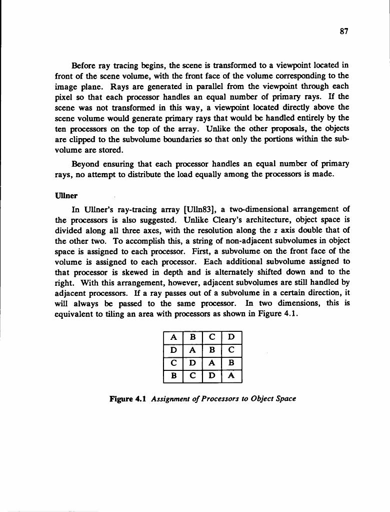
87

Before ray tracing begins, the scene is transformed to a viewpoint located in front of the scene volume, with the front face of the volume corresponding to the image plane. Rays are generated in parallel from the viewpoint through each pixel so that each processor handles an equal number of primary rays. If the scene was not transformed in this way, a viewpoint located directly above the scene volume would generate primary rays that would be handled entirely by the ten processors on the top of the array. Unlike the other proposals, the objects are clipped to the subvolume boundaries so that only the portions within the sub­volume are stored.

Beyond ensuring that each processor handles an equal number of primary rays, no attempt to distribute the load equally among the processors is made.

UllnerIn m iner’s ray-tracing array [Ulln83], a two-dimensional arrangement of

the processors is also suggested. Unlike Cleary’s architecture, object space is divided along all three axes, with the resolution along the z axis double that of the other two. To accomplish this, a string of non-adjacent subvolumes in object space is assigned to each processor. First, a subvolume on the front face of the volume is assigned to each processor. Each additional subvolume assigned to that processor is skewed in depth and is alternately shifted down and to the right. With this arrangement, however, adjacent subvolumes are still handled by adjacent processors. If a ray passes out of a subvolume in a certain direction, it will always be passed to the same processor. In two dimensions, this is equivalent to tiling an area with processors as shown in Figure 4.1.

A B C DD A B CC D A BB C D A

Figure 4.1 Assignment of Processors to Object Space

88

In this example, all rays that enter the subregion to the right of A enter the subregion handled by processor B.

Since the assignment of subvolumes to processors is skewed, extra connec­tions are required to connect processors at the outer edges of the array.

Thus, primary rays are distributed uniformly to each processor without hav­ing to transform the scene to the viewpoint. An implementation using 64 MC68000 processors each with 128K of memory is suggested.

Dipp6 and SwensenAnother architecture, suggested by Dipp6 and Swensen [Dipp84], relies

heavily on methods for load balancing. Since processors assigned to the regions of object space may not be uniformly-loaded, some method of adaptively redis­tributing these loads may be needed. Originally, the division of object space is uniform, but as processor loads change over time, space is adaptively resubdi­vided to produce more uniform loads. When a processor becomes heavily loaded during ray tracing, the load is reduced by changing the size of the assigned subvolume and redistributing the objects to other subvolumes.

Space is subdivided in three dimensions and assigned to a three-dimensional array of processors. The shapes of the subvolumes are not orthogonal, but are “general cubes” , cubes in which constraints about planarity of faces and convex­ity are relaxed. A two-dimensional analog is shown in Figure 4.2.

Figure 4.2 Two-Dimensional Analog of General Cubes

89

This shape was chosen so that the redistribution of loads would affect fewer processors than would be affected by moving the planes dividing space. Unfor­tunately, the shape makes clipping the objects to the subvolumes more difficult.

Processor loads are monitored and when a processor becomes too heavily loaded, redistribution is initiated. Load is redistributed by moving the comers of the cube, one at a time, until the load is sufficiently reduced. Of course, mov­ing a comer will affect the objects in eight subvolumes and hence eight proces­sors which share that comer. Therefore, these processors must be informed of the impending redistribution with a redistribution message sent from the loaded processor. Because processors should be informed of the redistribution as soon as possible, all processors act immediately on any redistribution messages in their queues.

After a number of redistributions, the subregion shapes may become very distorted, so that clipping and boundary testing are more difficult. When this occurs, a processor can change the shape so that it is more standard. While moving comers of cubes distorts the shapes, the advantage is that adjacent subregions will always remain assigned to processors that are directly connected.

When processors cannot reduce their loads, they degrade gracefully by removing secondary rays with very small maximum contributions from their ray queues. Another solution globally reduces the depth of all ray trees.

Because the eyepoint is within the scene volume, the processor responsible for the subregion containing it must generate all primary rays and pass them to the appropriate subvolumes. Regions of the subimage for which pixel intensities must be accumulated are spread among the processors.

Dippé and Swensen propose implementing this adaptive subdivision of space algorithm on a system consisting of eight commercial processors, each with 250 to 500K of memory.

Nemoto and OmachiThe sliding boundary surface method [Nemo86] was also motivated by the

need for some sort of adaptive load balancing, with the algorithm based on the uniprocessor volume-subdivision algorithm of the ARTS ray-tracing system [Fuji86], discussed in Section 3.2.2.3. Once again, space is divided along the three axes and assigned to a three-dimensional array of processors. Each subvo­lume is an orthogonal parallelepiped composed of unit cubes. A three­

90

dimensional digital line, generated by a 3D-DDA [Fuji86], is used to find the unit cubes pierced by a ray within a subregion and to enter the next subregion. Because this is an incremental technique, it is efficient for traversing space.

To adaptively balance the processor loads, the faces bounding the subregions can be slid to move unit cubes from one subregion and processor to another so that objects within the subregions are redistributed. Before ray tracing begins, the axis along which the number of objects is most varied is selected as the driv­ing axis. Only the boundary surfaces perpendicular to this axis can be moved. When a processor becomes too loaded, the boundary is slid by one unit towards this processor.

Although the subregions remain as orthogonal parallelepipeds, there is a disadvantage. After boundary surfaces are moved a few times, adjacent subre­gions may no longer be assigned to directly connected processors and ray mes­sages will have to pass through intermediate processors. This situation is shown in Figure 4.3.

Figure 4.3 Processor Assignments after Load Balancing

Simulations have been run using 64 and 512 subregions. Results indicate that total computing time is reduced when the adaptive load-balancing algorithm is used. Depending upon the clustering of objects in the subvolumes, the time is four-fifths to one-quarter that using an algorithm without adaptive redistribution.

4.S.2.2. Load BalancingIn all proposals that divide the ray-tracing problem in this manner, some

attempt is made to equalize processor loads because the efficiency of the ray- tracing system is dependent on all processors being equally utilized. Two of the

91

proposals avoid overloading a few processors with primary rays, while the other proposals perform load balancing dynamically during ray tracing. In such dynamic strategies, a variety of factors must be considered when selecting an optimum algorithm.

Distributing Primary RaysTo begin ray tracing, primary rays are generated and passed to the proces­

sors responsible for the first subvolumes that the rays enter. Depending upon the subdivision of object space and the physical arrangement of the processors, cer­tain processors may be overloaded with primary rays while others receive none.

If the viewpoint is contained within the scene volume and assigned to one processor [Dipp84], this processor must intersect each primary ray with every object in the subvolume before passing the ray to the processor assigned to the next subvolume. These processors will also be overloaded until secondary rays propagate through the subvolumes to the other processors.

If the viewpoint is located outside the scene volume, the distribution of pri­mary rays is dependent upon the assignment of processors to subvolumes. When object space is divided in two dimensions and assigned to a two-dimensional array of n 2 = N processors, n Xn processors are represented on the front and back faces of the scene volume, while only n are on all other faces. A viewpoint located directly above the scene will send primary rays to only n processors pro­ducing a ratio of working to idle processors of .

When object space is divided in three dimensions and assigned to a three- dimensional array of n 3 = N processors, n X n processors are represented on each face of the scene volume. For most viewpoint locations, approximately n 2 processors receive primary rays, changing the ratio of working to idle processors

to 3̂ TGenerally, three-dimensional division and assignment is better at distribut­

ing the primary rays over the processors. Consider an implementation using a total of sixty-four processors. In two-dimensional subdivision, eight processors must handle all primary rays while in three-dimensional subdivision, sixteen pro­cessors handle the primary rays.

92

Uniform distribution of the primary rays is addressed in two proposals, both of which use a two-dimensional array of processors. In one method, the scene is first transformed to the viewpoint so that all primary rays enter the scene through the front face of the scene volume [Clea86]. Consequently, the same number of rays is handled by each processor in the system. An alternate approach divides space along all three axes and skews the assignment of cubes to processors so that a processor is represented an equal number of times on each face of the scene volume [Ulln83]. Although some viewpoint positions will cause a few processors to receive more rays than others, in general, this algo­rithm performs well.

Dynamic Load BalancingThe two other proposals perform load balancing after ray tracing has begun

[Dipp84, Nemo86]. The only way to redistribute loads is to change the size of the subvolumes handled by the processors, so that objects are moved from a highly loaded processor to one that is more lightly loaded.

Some operations are common to every dynamic load-balancing algorithm. Load metrics, measures of the utilization of processors, must be calculated and exchanged by neighbouring processors so that a processor can decide whether or not to reduce its load and to which neighbouring processors that load should be given. Once a processor initiates a redistribution, it must decide how to move the boundaries of the subvolume and notify each affected processor of the new boundaries. All processors must then clip objects that now fall into their space to the new boundaries of the subvolume.

These two proposals differ in a number of respects. The shapes of the sub­volumes and the number of processors affected by a redistribution are important. As well, the simplicity of deciding how to reduce the processor’s load and the redistribution of the objects in the affected subregions are different. A final con­sideration is whether adjacent subregions remain assigned to connected proces­sors. Because these decisions affect the amount of time that must be spent run­ning load balancing, they are important considerations in developing a load­balancing algorithm.

When selecting a shape for the subregions, certain factors must be addressed. The first is the ease of clipping the objects to the volume boundaries and the second is the ease of determining if a point is inside a subvolume.

93

In one proposal, subregions are “general cubes” , six-sided subvolumes that may be concave and have non-planar faces, formed by moving comers of a cube in any direction in three-space [Dipp84]. In the other proposal, subregions are orthogonal parallelepipeds composed of unit cubes [Nemo86]. Subvolumes are altered by moving a sliding boundary surface by one unit cube towards the loaded processor.

Clipping is easiest when performed against a standard clipping volume. With parallelepipeds formed from unit cubes, clipping objects to subvolumes is simple. For general cubes, clipping is more difficult because the volume may be concave and the sides may be non-planar. Each face will need to be divided into two planes because the face is defined by four non-coplanar points and objects will need to be clipped to twelve planes instead of the usual six. As well, processors that share subregion boundaries must split the face into the same two planes to ensure that no objects are missed.

In addition to the clipping consideration, it should be easy to determine if a point is within a particular subvolume. This is necessary to ensure that intersec­tion points lie within the subvolume belonging to the processor and to determine if the next subvolume a ray enters is still assigned to the processor. If load redis­tribution has occurred after a ray message is generated, the processor may no longer be responsible for that point. Therefore, when processors receive a ray message, they must first check that the point is in their subvolume. Of course, it is simpler to test orthogonal parallelepipeds than general cubes because of their shapes.

When a load redistribution is initiated, the number of subvolumes, and hence processors, affected should be kept to a minimum. If many processors are affected, each processor will have to change subregion boundaries and reclip the objects to the new subvolume, increasing the cost of load balancing. For sliding boundary surfaces, only one other processor is affected by a redistribution, but with general cubes, seven other processors are affected when a comer of the cube is moved.

A processor that is very busy may have to make many decisions in order to reduce its load. Primarily, this involves calculating the amount of load to be given away, to which processors this load should be given, and, more impor­tantly, deciding how to change the subvolume’s shape to accomplish this. When such decisions are complicated, the processor will spend a significant time run­ning the load-balancing algorithm, reducing the time available for ray tracing.

94

For general cubes, the processor initiating the redistribution must first select one of the eight corners of the subvolume to move. Because a corner can be moved in any direction, the processor must determine how far and in which direction to reposition the comer to reduce the load of the processor and distri­bute the load to the affected processors in proportion to their loads. Thus, this algorithm can become quite complicated.

In contrast, the sliding boundary surface method is very simple because most decisions are made statically. The plane of the boundary surface is chosen before ray tracing begins and is the same for all processors. It is simply the plane perpendicular to the axis along which the number of objects is the most varied. When a processor initiates a redistribution, it must only select one of two boundary surfaces to move and always slide the surface by one unit cube towards the processor.

When a processor initiates a redistribution, the processors affected must be notified of the change in subregion shape so that they can clip all objects that possibly intersect their subregions to the new boundaries. If objects can come from any affected subvolume, as in the general cube method, all affected proces­sors must exchange object lists. The sliding boundary surface method is simple because only two processors are affected, with the objects coming only from the initiating processor.

Originally, object space is divided so that adjacent subvolumes are assigned to connected processors. Since rays pass from one subvolume into an adjacent subvolume, messages can be sent directly between the two processors. When dynamic load balancing is performed, the change in subvolume shape may cause adjacent subvolumes to no longer be assigned to connected processors, so that ray messages will have to pass through intermediate processors before reaching the desired destination.

Adjacent general cubes will always remain assigned to connected processors because only the positions of corners are changed. Although the shapes of the cubes may become very distorted, the passing of ray messages will remain sim­ple. However, in the sliding boundary surface method, adjacent subregions will quickly become disconnected. When a boundary surface is slid, four processors will be indirectly affected because rays leaving their subvolumes may no longer pass into the subregion handled by the connected processor. When this happens, rays will have to pass through intermediate processors. Because the unit cube number that the ray enters is known, routing of the message is very simple.

95

However, subvolumes assigned to processors along the axis perpendicular to the sliding boundary surface will always remain connected.

Many of these preceding features are desirable for a dynamic load-balancing algorithm. The shapes of the subvolumes should be such that objects are well contained and cross few subregion boundaries. The shape should also allow objects to be clipped easily to the boundaries. As well, the shape should remain relatively undistorted throughout the load-balancing process, allowing objects to be clipped easily to the boundaries.

To accomplish load balancing efficiently, processors should be required to make as few decisions as possible so that the least processor time is taken away from the intersection of rays with objects. In addition, the number of subvo­lumes affected by the redistribution should be minimized. With fewer affected processors, less information must be exchanged by the processors and fewer pro­cessors must perform redistribution operations. Finally, the load-balancing algo­rithm should allow adjacent regions of space to remain assigned to connected processors. Otherwise, ray messages will have to be processed and forwarded by intermediate processors.

The sliding boundary surface method proposed by Nemoto and Omachi is the better dynamic load-balancing method in all respects but one: ray messages will have to pass through intermediate processors. However, along one axis, subregions will still remain assigned to connected processors and ray messages destined for other processors can be easily forwarded. General cubes, suggested by Dippé and Swensen, have very distorted shapes requiring processors to make complicated decisions when initiating ray tracing. The shapes also complicate the clipping of the objects to the boundaries of the subvolume. All of this is compounded by the large number of processors affected by each redistribution. Compared to sliding boundary surfaces, this scheme has a much higher over­head.

4.6. Chapter SummaryVarious parallel architectures that introduce parallelism into the ray tracing

algorithm have been designed. Vectorization is used to test many rays for inter­section with the same object in parallel. Pipelining, in which the ray tracing algorithm is divided into a number of stages performed by additional processors or separate circuitry, has also been used. The ray-tracing peripheral uses pipe­lining to stream a succession of objects past a single ray. In the ray-tracing

96

pipeline, rays are passed through a pipeline of processors, each of which is assigned to an object in the scene. Finally, multiple processors can be assigned to either regions of image space or object space.

For a ray tracing system, a number of necessary features and acceleration techniques have been identified. These include modeling the scene with multiple primitives, including those with iterative intersection tests and fractal surfaces. Texture mapping should be possible. Distributed ray tracing to model blurred phenomena is also important and antialiasing through either uniform or stochas­tic sampling is necessary.

Acceleration methods should also be incorporated into parallel architectures for ray tracing. Bounding volumes and scene-structuring techniques are very important in uniprocessor ray-tracing algorithms. As well, tree-depth control and ways of reducing shadow testing time should be included.

Not all features and acceleration techniques are easily incorporated into the design of the parallel architectures. However, the most flexible architectures appear to be the multiprocessor systems. Detailed issues for multiprocessor sys­tem are examined in the next chapter.

Chapter 5

Multiprocessor Ray Tracing Issues

When analyzing the multiprocessor ray-tracing methods that divide the problem in image space or object space, a number of important factors must be considered. Each method has both advantages and disadvantages. Unless cer­tain decisions are made about the types of images that the system is required to render and the budget available for the system, it is not clear which method of subdivision is superior.

Some factors involve constraints on the physical construction of the architec­ture including the amount of memory required and available on each processor, communication requirements and overhead, and the overhead of initializing each processor. As well, recovery from failures and methods of load balancing have an impact on the efficiency of such a system. Because these factors impose extra constraints, the observed performance of the system may not reach the predicted theoretical performance.

In addition to the efficiency of the subdivision methods and their implemen­tations, each system should be able to implement the features and the accelera­tion techniques which have been incorporated in the uniprocessor ray-tracing algorithm.

5.1. System IssuesMemory requirements are important in multiprocessor systems since each

processor usually has a limited amount of local memory to which it has exclusive access. For ray tracing, in which a large amount of memory is required for the rendering code, object descriptions, scene data structures and texture and bump maps, the amount available may be critical to the efficient operation of the sys­tem. More memory is required by the processors in image-space subdivision because each processor needs access to the entire scene, unlike object-space sub­division, in which processors only need to store objects that intersect the assigned volume.

97

98

Communication overhead is another factor that is important in multiproces­sor systems. In an image-space subdivision implementation, little or no com­munication is required among the processors. Each processor operates auto­nomously and requires no information from other processors in order to render a pixel of its subimage. On the other hand, object-space subdivision has a large amount of interprocessor communication because rays traveling through object space are modeled as messages passed among the assigned processors. There­fore, a message is generated for every ray created during the rendering of a frame with the result that communication overhead may not be insignificant.

The communication requirements also tend to dictate the physical arrange­ment of the processors. In multiprocessor systems that perform a great deal of interprocessor communication, direct links between communicating processors are advantageous. Since processors in image-space subdivision do not need to communicate, the way in which the processors are connected is not affected by these requirements. However, processors in object-space subdivision with much interprocessor communication are organized so that processors handling adjacent regions of space are physically connected.

Because ray tracing is frequently used to render images for animation, any overhead present in initializing the processors before ray tracing begins is magni­fied if it must be performed again for each successive frame. Necessary initiali­zation includes downloading the ray-tracing object code to the processors and transferring object and scene descriptions to processor memory.

Load balancing, which distributes work so that processors are fully and uniformly-loaded, is another major issue for multiprocessor systems. If some processors are idle while others have been given too much work, the maximum speed-up cannot be attained since full multiprocessor utilization is achieved when all processors are executing continuously. Ray-tracing algorithms, when imple­mented with multiple processors, are inherently poor in providing equal loads to the processors.

Since the time to ray-trace a scene depends on the time for the slowest pro­cessor to finish tracing the last ray, some form of load balancing is necessary to attain the maximum speed-up. However, any overhead generated by the load­balancing algorithms must be considered when comparing the two subdivision methods. Generally, load balancing is more difficult for object-space subdivision than for image-space subdivision.

99

5.1.1. Memory RequirementsMemory requirements are a critical consideration in both image-space and

object-space multiprocessor ray-tracing systems. This is also true of any distri­buted system in which the application requires a large amount of storage. The memory requirements for ray tracing may also affect how the processors are con­nected and the communication requirements and overhead for the system. When determining whether processors should be assigned to regions of image space or regions of object space, the amount of memory needed may be the determining factor.

Ray tracing has very heavy memory requirements. In a uniprocessor ray­tracing system, real memory is required for the ray-tracing code, object descrip­tions, scene data structures, and texture and bump maps. As an indication of the amount of memory required by each of these, consider a ray tracing system implemented on a VAX-11/780 at the University of Waterloo [Swee84]. In this implementation, which handles many different primitives including spheres, cylinders, polygons, fractals and B-spline surfaces, all of which may be texture mapped, approximately 30K bytes is needed to store the object code, with 16K bytes of this required for the intersection routines. For most images rendered by this ray tracer, total memory necessary ranged between 4 and 10 megabytes. One complex scene of texture-mapped fractal mountains bordering a reflective lake needed 24 megabytes of virtual memory in which to run and used 228 minutes of cpu time. However, one reason that so much storage was needed was that the fractal hierarchy was fully instantiated in a preprocess phase. Therefore, memory requirements would normally be under 10 megabytes.

In all of the proposed multiprocessor solutions for both image- and object- space subdivision, the processors used are commercial microprocessors such as MC68000’s, each with between 128K bytes and 1 megabyte of on-board memory. Certainly, the amount of memory required by a processor in the sys­tem depends upon many factors arising from the subdivision method. However, using such a small amount of memory may impose unnecessary restrictions on the architecture and capabilities of the ray-tracing algorithm.

A multiprocessor solution is sought for ray tracing in order to parallelize the calculations, thereby reducing total execution time. Ray tracing times will need to be reduced if scenes are very complex or if many images need to be rendered. This implies a production environment in which many capabilities of the above uniprocessor system will be required to render complex scenes. Consequently,

100

such memory requirements of 4 to 10 megabytes will be typical for a ray tracer capable of producing these types of images and these numbers will be used in analyzing memory requirements for each subdivision method.

For each of the subdivision methods, the amount of information that each processor must have access to is the determining factor in the amount of real memory required by a processor. If not enough local memory is available, shared memory or disk storage may be necessary. However, when such alterna­tives are used, memory access times will increase, reducing the efficiency of the multiprocessor system. Some of these alternatives have been suggested to reduce the effects of limited memory in some proposals.

5.1.1.1. Image-Space SubdivisionMemory requirements for image-space multiprocessor ray-tracing system are

very large because each processor must have access to the object descriptions and the data structure describing the entire scene. Each processor executes the same ray-tracing algorithm as a uniprocessor ray tracer, with the only exception being that each operates on a smaller subimage. Ideally, all data to which the processors require access should be stored in local memory to keep memory access times as low as possible. Since processors require such a large amount of memory, commercial processor boards with typically small amounts of memory cannot be used.

Each processor must store in local memory the object code for the entire ray-tracing algorithm, which should require less than 30K bytes of memory. As well, processors must have access to all object descriptions, the data structure describing the scene, and the texture and bump maps. Typically, the amount of storage required ranges from 4 to 10 megabytes. Texture and bump maps alone consume a large amount of storage; a 512 by 512 map requires 1 megabyte while a larger 1024 by 1024 map needs 4 megabytes. If objects are textured with different maps, the amount of storage required will be significant.

Processors must also store the intensity values calculated for the pixels in the subimage. If a pixel intensity is returned to the host as soon as the value is known, storage for only one pixel is needed. However, if the pixel intensities are returned after the entire subimage is computed, more storage will be neces­sary.

101

Besides storing all the required information in local memory, other possible alternatives have been suggested, including shared memory and disk storage, although both have increased memory access times. Because the ray-tracing algorithm is cpu-bound and storage-intensive, such alternatives should be avoided. Object and scene descriptions are accessed very frequently by each processor because of the number of ray-object intersections that are performed and the frequency of memory accesses during the traversal of the data structure. Thus, memory access times will be kept to a minimum by storing this informa­tion in real memory.

Texture maps are not accessed as often and consequently are candidates for shared memory or disk storage if not enough local memory is available. Unlike object descriptions, texture maps are accessed only when a textured object is found to be a visible surface. Unfortunately, if texture maps are stored on disk, disk i/o requests for texture map values must be sent to the host. The host will be required to manage queues of disk requests, resulting in extra overhead for all processors. Therefore, disk storage should be avoided.

Pixel intensity results are always stored in real memory until they are transmitted to the host. If processor memory is small, results can be transmitted more frequently to reduce the storage requirement.

Two choices are available for the organization of main memory, each of which has advantages and disadvantages: local memory and shared memory. Local memory, located on the same board as the microprocessor, is accessed exclusively by that processor. Shared memory is accessible by all processors in the system. The selection of one over the other is dependent upon cost and memory access time.

Storing the scene data structure, object descriptions and texture maps in memory local to each processor has one important advantage: memory access time will be minimized as there is no contention with other processors. How­ever, commercial boards are not equipped with enough on-board memory to accommodate the large storage requirements of up to 10 megabytes. Thus, cus­tom processor boards with large on-board memory will be required.

Most commercial microprocessors can accommodate the large amount of memory because the virtual address space is large. MC68000’s have 24-bit addresses, accommodating 16 megabytes of real memory while the newer MC68020’s have 32-bit addresses, allowing up to 4 gigabytes of memory. Since

102

most scenes require between 4 and 10 megabytes, memory addressing is not a constraint.

Depending upon the chip size, it may be physically impossible to place enough chips on a single board to make up this amount of memory. If 2S6K chips are used, 32 chips are needed for each megabyte, with 320 needed for 10 megabytes. If larger chips, such as 1 megabit chips, are used to reduce the number of chips that must be placed on a single board, only 80 are needed to make up 10 megabytes of memory. However, there are two disadvantages in using these larger chips: the chips have two extra pins, making them difficult to mount on standard processor boards, and they are costly.

As mentioned, it takes 320 256K chips to make up 10 megabytes. Assum­ing that each chip costs approximately $4, the cost of memory for one processor is $1,280. However, for 1 megabit chips costing about $25 each, the same 10 megabytes will cost $2,000. Since this amount of memory is required for each processor, the cost will be magnified by the number of processors. For example, memory for 64 processors will cost either $81,920 using 256K chips, or $128,000 using 1 megabit chips. At this point, there is a tradeoff between the funds avail­able for purchasing local memory and those used to purchase processors. There­fore, if processors are to be supplied with large local memories, the total number of processors in the system may have to be reduced, decreasing the parallelism in the system.

While using a large amount of local memory on each processor is the optimal solution when considering system performance, it may be prevented by the above limitations. The real disadvantage of using local memory, however, is that the object descriptions and scene data structures, which occupy the most space, must be replicated in each of the memories. If all processors could access one copy of this data stored in a shared memory, less memory in total would be required, thereby reducing the cost. Each processor would still use local memory to store the code needed for ray tracing, but would access shared memory for the object descriptions, scene data structures, and texture maps.

The use of shared memory, however, has its disadvantages. Memory access times for the processors will increase for two reasons: memory is not physically as close as on-board memory and contention for access to memory will develop among the processors.

103

As soon as memory that must be accessed by a processor is not on-board, access time will increase because of delays caused by the physical distance separating the processor from memory.

Depending on the way in which the processors are connected to memory, delays may be costly. If processors and memory are connected via a bus, access may initially be fast because of the bus speed, but contention for the bus and memory will increase memory access time. Since processors perform many memory accesses, contention will be a problem that must be addressed in the system. Instead of consolidating memory in one location, shared memory can be distributed over the processors, with requests for access transmitted over a bus. However, bus contention will also be a problem with this organization. Also, memory could be attached to and managed by a single processor, with all pro­cessors connected to this processor by serial lines.

One serious disadvantage of shared memory is that contention arises when many processors attempt memory accesses simultaneously. A processor wanting to access memory may first have to wait for other processors to finish their memory accesses before it can proceed, thereby increasing memory access time. To ensure that requests for memory access are handled fairly, an arbitration scheme that queues and then processes the requests in the order that they are received is necessary. As the number of processors in the system is increased, the contention problem becomes magnified.

Contention is a major factor in using shared memory for ray tracing because of the frequency with which processors must access the object descriptions and scene data structures. A good portion of time in ray tracing is spent determining the closest object that a ray intersects. Fortunately, processors only need to per­form reads, not writes, from this shared memory, so that access time is minim­ized.

When a choice is made to use local or shared memory, the main tradeoff is the speed of memory access versus the cost of memory. A system in which each processor has enough local memory to store all the necessary information to which it requires access will have very fast access times. However, this amount of memory is costly because the same information must be replicated in each processor. A shared memory system can be used for the very reason that each processor must access the same information. Thus, less memory in total is required, thereby decreasing memory cost. However, access times for a shared memory system will increase because there is contention among the processors

104

for access to memory. As well, an arbitration scheme is required. If the cost of memory is deemed not to be important, each processor should be supplied with enough local memory to store all information required during ray tracing.

Another solution combines shared memory with local cache. Because pro­cessors require only read access to memory, the organization is ideal for this application. Of course, there must be some locality of reference for efficiency. While processors are traversing the data structure, the next location accessed is usually predictable and stored nearby in memory. As well, the local cache can consist of those object descriptions that project onto the assigned subscreen. Because these objects will be intersected by the primary rays, they are ideal for local cache. Such a memory design should be investigated further as it will reduce the number of accesses to shared memory, which in turn may make shared memory more feasible.

As well, it should be noted that in a commercial multiprocessor system with shared memory, contention problems for memory accesses will already have been addressed and access times minimized. Consequently, this system may be more expensive, but the cost must be weighed against the cost of using local memory.

5.I.I.2. Object-Space SubdivisionWhen object space is divided and assigned to many processors, memory

requirements are not as critical to the operation of the system. For each subvo­lume that is created, the processor requires access to less information and conse­quently, needs less storage.

Because the ray-tracing algorithm is divided in object space, only those objects that intersect the subvolume to which the processor is assigned need to be stored in memory. The processor does not need access to any other object descriptions in the scene. In addition, when the number of objects in a subvo­lume is small, no other form of scene structuring is required, eliminating the need to store any other data structure.

If there are M objects and N processors, each processor will require storage Mfor approximately — objects, thus spreading the total storage required for the

descriptions over all of the processors. Although it has been shown that objects are usually not uniformly-distributed throughout space [Whel86], this ratio is still

105

a fairly good approximation for the number of objects in each subvolume and therefore the amount of storage required. Also, when a primitive intersects more than one subvolume, its description will be duplicated in each processor. Of course, for more processors in the system, less memory is needed for each.

As well as the reduction in the number of object descriptions that must be stored, the amount of ray-tracing code will be reduced because processors do not implement the entire ray-tracing algorithm. This algorithm is controlled by the host, with processors mainly responsible for intersecting rays with objects in the subvolume. Typically, intersection routines will require about 16K bytes of memory. However, more code will be necessary for passing ray messages among the processors and possibly for performing dynamic load balancing.

Additional storage will be required in some or all processors for the intensity values for subimages of pixels. If this memory can be spread over many or all processors, it will not be significant.

Since each processor needs access to significantly less information than a processor in the image-space subdivision method, each should use local memory exclusively in which to store the rendering code and object descriptions. This should not require much more than a few megabytes of memory and will there­fore be relatively inexpensive to put locally on each processor.

Some processors, storing objects that are texture- or bump-mapped, will need access to the appropriate maps. When textured objects appear in more than one subvolume, or one object appears in many subvolumes, more than one processor will need access to these maps. For the cost of a few more megabytes, texture maps that might be needed for an object in the subvolume can also be stored in local memory. Or, since access to texture maps is infrequent, occur­ring only if the textured object is found to be the visible surface, the map could be spread over a number of processors and accessed by sending a message to the appropriate processor.

In all proposed implementations of object-space subdivision, processors have between 128K and 500K bytes of local memory. This will not be sufficient, even for the reduced memory requirements. However, assuming that processors will require about 2 megabytes of memory, 256K chips can be used which will cost about $256 per processor. When the array contains 64 processors, the total cost will be $16,384.

106

5.I.I.3. Comparison of StrategiesMemory requirements for object-space subdivision are simpler than those for

image-space subdivision. Since processors assigned to regions of object space need access to less information, less local memory will be required, thereby reducing the cost of the system. In image-space subdivision, a very large amount of memory is required because each processor needs access to all object descriptions and the entire data structure describing the scene. Thus, these pro­cessors can use either shared memory, in which contention and physical separa­tion may increase memory access time, or local on-board memory, which may be very expensive.

5.1.2. Load BalancingLoad balancing, a technique that distributes the load evenly to the proces­

sors, is necessary for multiprocessor systems. Otherwise, the potential speed-up of using additional processors may not be realized. During the execution of any algorithm that has been distributed over many processors, some processors may receive more work than others, leaving some processors idle while others are overloaded. A load-balancing method attempts to divide the computations so that processor loads are more balanced.

In multiprocessor ray-tracing systems where the algorithm is divided and assigned to many processors, load balancing is also important because the loads of the processors can vary. While load balancing will improve the efficiency of the processors by ensuring that work is distributed equally, the method adds overhead in terms of additional processor and communication time. This over­head must be considered when selecting a load-balancing algorithm for ray trac­ing.

Multiple processors are usually applied to a problem to reduce the total exe­cution time by having many machines work in parallel. Under ideal conditions, in which each processor is fully utilized, the greatest speed-up that can be achieved is N, where N is the number of processors in the system. However, this full speed-up will rarely be attained because some processor overhead is usually introduced by reorganizing the computations. Processors will sometimes execute code that does not relate directly to the solution of the assigned task.

107

In addition to this algorithm overhead, the system will not achieve full speed-up if the processors are often idle or if the processor loads are not uniform. Processors can become idle if they receive a very small amount of work com­pared to other processors or because work arrives only intermittently. In a sys­tem where M processors are executing while the other N — M processors are idle, the algorithm would be sped up by only a factor of M, which could have been achieved with M fully utilized processors. Since a multiprocessor algorithm relies on all processors performing necessary computations in parallel, non­uniformity of loads will increase the total ru nn ing time for the application.

To eliminate or at least reduce this inequality of work, load-balancing methods are used. Ideally, the computations should originally be distributed among the processors so that each receives the same amount of work. However, in many algorithms, it is not possible to accurately predict processor loads before the processors begin executing. Even if the computation is initially divided so that processors receive equal loads, the loads may change over time due to the nature of the algorithm being executed. In these situations, methods that equal­ize the loads by redistributing the computations dynamically will be needed to move computations from heavily-loaded processors to ones that are more lightly loaded.

There are many examples of load balancing in distributed systems. Con­sider a simple system in which many processors are available to run jobs. Instead of dedicating one processor to each user, processors are pooled and allo­cated as they are needed. If each processor has identical hardware and software, jobs need not be run on a specific processor, but can be run on any processor that is not being used. In this way, certain processors are not over­loaded with jobs submitted by one user, while other processors remain idle. Loads are balanced because work can be assigned to any processor that would otherwise be idle.

In another system in which many tasks execute on the different processors, load balancing can be performed while the processors are executing. When a processor is identified as having too much work, its load can be redistributed by moving tasks from this processor to one that is lightly loaded. Code, data, and a copy of the run-time stack are moved to another processor, where the task can be restarted.

108

Load balancing in both examples of distributed systems is simple because the tasks on one processor are independent of each other as well as of those assigned to other processors. When computations assigned to one processor depend in some way upon other processors, load balancing is more complicated.

Multiprocessor ray-tracing systems also require some method of load balanc­ing for efficiency because both divisions of the ray-tracing computation have aspects that result in non-uniform processor loads. Image-space subdivision pro­duces subimages that have very different complexities and, therefore have very different computation times. Object-space subvision produces regions of space with varied numbers of objects through which different numbers of rays pass, resulting in different numbers of intersection tests and very non-uniform proces­sor loads.

When the ray-tracing computation is divided in image space and a subimage assigned to each processor, some subimages will be more complex than others and will require more time to ray-trace. The complexity of a subimage is meas­ured by the number of rays that must be traced to calculate the pixel intensities. For some pixels, the ray trees will not be very large because only a few rays have to be traced, but for other pixels ray trees will be very deep because many reflective or refractive objects are encountered. When a subimage is composed primarily of pixels that are either very simple or very complicated, the assigned processor will take a considerably different length of time from the average. If two subimages are compared, one in which most pixels are background and a second in which most are covered by a reflective object, the second processor will take many times longer to complete than the first.

While it would be convenient to assume that all the subimages are equally complex and processor loads are equal, this is not true in practice. When no attempt is made to equalize the work of the processors, the image plane is sim­ply divided into the same number of subimages as processors, with each proces­sor ray-tracing one subimage. For the final image to be generated, each subim­age must be computed. Only when all processors have completed will the final picture be available. Hence, this multiprocessor system is only as fast as the slowest processor. When processor loads are extremely varied, efficiency is lost because processors remain idle waiting for the slower ones to finish. Therefore, some load-balancing method must be used to distribute the work equally among the processors.

109

In object-space multiprocessor ray tracing, loads of the processors are also likely to be varied. The complexity of the work assigned to a processor depends primarily upon two factors: the number of objects in the subvolume and the number of rays that pass through the subvolume. Because a processor must intersect each ray entering its subvolume with every object, many objects and rays generate a high work load. In fact, if either the number of objects or number of rays is high, the load will also be higher than average. The complex­ity of the ray-object intersection test is also important. Reflective and refractive properties of the objects will contribute to the load since secondary rays have to be generated and processed for each intersection point.

A processor will be idle most of the time if its subvolume contains no objects and rays rarely enter the subvolume. On the other hand, a processor may have been assigned a subvolume that contains many objects and through which many rays pass. For instance, many rays will enter a subvolume containing a light source because a shadow ray aimed at this subvolume is generated for each intersection point. A processor can also be highly loaded if it must process an extraordinary number of rays. If a subvolume is located directly between two subvolumes containing highly reflective objects, many rays may pass between these objects through the subvolume, thereby raising the processor’s load.

It is difficult to predict the load of a subvolume, partly because the number of rays that must be handled by a processor is not known. As well, the loads of processors can change over time. A processor that is overloaded just after ray tracing has begun may have a small workload later on. Another reason that predicting the loads is difficult is that the input for one processor is dependent upon the output of other processors as a processor will have no work unless a ray that passes through its subvolume has been previously generated by an intersec­tion in another processor.

When processors have varying loads, some can be idle while others have queues of rays waiting to be processed. In such situations, processing power is lost because not all processors are working. Once again, all processors must complete before the image is formed and therefore, the system is only as fast as the slowest processor. For this reason, it is important that the loads of the pro­cessors be equal. To properly distribute the loads, some form of load balancing must be used for the division of the problem in object space.

110

Methods of load balancing a distributed system are as diverse as the applica­tions executing on the processors. Despite the differences, the load-balancing algorithms can still be classified as either static or dynamic, depending upon when load redistribution is performed. For dynamic load-balancing algorithms, control can be centralized or distributed and the effects of redistribution are either local or global.

If a load-balancing method is static, the computation is divided as evenly as possible and assigned to the processors before execution. At no time during exe­cution are the loads of the processors changed by redividing the computation. Therefore, the loads of processors must somehow be predicted before execution time.

On the other hand, a dynamic load-balancing strategy is run periodically while the processors are working on their assigned computations. Whenever non-uniformity of processor loads is detected, some of the load can be moved away from heavily-loaded processors to ones that currently have less work. Unfortunately, a dynamic load-balancing strategy is more complicated and has more overhead than a static strategy. However, it is more effective in keeping the loads of processors uniform. If a static strategy is not accurate in predicting processor loads, nothing can alter the loads later on. When static and dynamic load-balancing algorithms are combined, the problem is originally divided so that processors receive equal loads and work is later redistributed if processor loads are found to vary.

In a static load-balancing method for ray tracing, a means of predicting the loads of the processors is needed. At the beginning of each frame to be ray- traced, image space or object space is divided so that work is assigned as equally as possible based upon certain characteristics of the scene. After the processors begin execution, no redistribution is performed. While static load balancing may be easy for some applications, it is not easy for ray tracing because loads cannot be accurately predicted before ray tracing begins.

A dynamic load-balancing method for ray tracing redistributes load while the processors are executing. Processor loads are monitored during ray tracing and any time a processor is found to be overloaded, part of its work is given to other processors. In image-space subdivision, pixels to be traced are moved from one processor to another and in object-space subdivision, parts of subvolumes are moved.

I l l

Control of the dynamic load-balancing algorithm can be either centralized or distributed. This determines where the load-balancing code is executed and which processor or processors make the decisions about when to redistribute load and how to redivide the computation. If the algorithm is centralized, one pro­cessor monitors the loads of all processors in the system and initiates redistribu­tion when necessary. If the algorithm is distributed, any processor can initiate load redistribution when its own load becomes too high relative to that of other processors.

The effects of performing dynamic load balancing can be local or global depending upon the number of processors affected by a redistribution. With a global load-balancing algorithm, computations are completely redistributed so that all processors are affected. Often, a global method reduces the loads of all processors by simplifying the work required of each. On the other hand, when only one processor has too much work, a more localized algorithm redistributes the load among only a few processors.

While load balancing more evenly distributes the computations to the pro­cessors, thereby improving the efficiency of the system, it is not without cost. Time must initially be spent dividing the problem and then again performing redistributions since processors must leave the task to which they have been assigned to execute the load-balancing code.

Load-balancing overhead can be in the form of processor or communication overhead. Processor overhead results from running the load-balancing algo­rithm. Whenever load equalization is being performed, processors cannot be working on the tasks to which they are assigned. Communication overhead refers to additional communication that must occur between processors in order to accomplish load balancing.

Whenever load balancing is considered for a multiprocessor system, the effi­ciency that is recovered by performing the redistribution must be weighed against the cost of the load-balancing algorithm. For some algorithms, the cost in terms of additional overhead can be very high, especially for dynamic load balancing. In some cases, the time lost from running the load-balancing algo­rithm may be more than the time gained by having a more uniformly-loaded system. At this point, there is no advantage in performing load balancing. In the worst case, a processor may be continuously dealing with redistributions and never be free to perform its assigned work. Thus, load-balancing overhead must be minimized.

112

5.1.2.1. Image-Space SubdivisionLoad balancing for the image-space multiprocessor ray-tracing system is

relatively simple. Initially, the image is divided into many more subimages than processors so that each processor is assigned one of these small subimages. As soon as a processor finishes ray tracing its subimage, it is assigned another por­tion of the frame to render. Once a processor begins ray tracing a subimage, it never becomes idle until the subimage has been computed; it does not need to wait for another processor that has been given a complex task to finish.

In many ways, this load-balancing algorithm is similar to load balancing in a distributed system of processors executing user jobs in any order. Subimages are equivalent to jobs that are assigned to any processors that become idle.

As well, additional opportunities for load balancing exist when images to be ray-traced are part of an animation sequence. If one frame need not be com­pleted before tracing of the next frame begins, subimages from the next frame can immediately be given to idle processors. Otherwise, idle processors must wait for the others to finish the subimages for that frame before they receive any more work. Because this idle time occurs at the end of each frame of the sequence, it rapidly accumulates to reduce the efficiency of the multiprocessor system. With load balancing in animations, some processors will be idle only once at the end of the last frame.

Before this extension to load balancing can be used, certain criteria must be satisfied. The frames that are being ray-traced must eventually be displayed and recorded on film or tape, but if the frames are being displayed and recorded as they are being ray-traced, a new frame cannot be started before the first has fin­ished. However, if the ray-traced images are being stored on disk and recorded at a later time, ray tracing of another frame can begin before the current one has been completed. Even in this case, processors must have access to the data for the new frame. If the scene description does not change and only the viewpoint moves between frames, processors can easily ray-trace different frames simultaneously. However, if the scene description changes, a shared memory system will not have enough space in which to store more than one frame. So, only if each processor has its own memory will this additional load balancing be possible.

113

This load-balancing algorithm is difficult to classify as static or dynamic. In one sense, it is static because the problem is divided only once and after this ini­tial division, the subimages are never changed. However, these subimages are assigned dynamically to the processors during the ray tracing of a frame. Thus, the algorithm is a hybrid scheme, combining some aspects of static load balanc­ing and some of dynamic.

Control of this load-balancing algorithm is centralized, usually performed by the host which initially downloads the code, scene descriptions and viewpoint to the processors and assigns the subimages. When a processor becomes idle, sig­naled by the return of the rendered subimage, the host knows to assign a new subimage. For this reason, the calculation of a load metric is unnecessary. As well, since only one processor, an idle processor, is affected when a new subim­age is assigned, the algorithm effects are very localized.

A purely dynamic load equalization method divides the frame into the same number of subimages as processors. While the processors are ray-tracing subim­ages, unfinished pixels are moved from overloaded processors to processors that have become idle. Such a scheme incurs a greater cost than the load-balancing method discussed previously since some means of monitoring processor loads and communicating the redistribution information to the affected processors is needed. An entirely static method of load balancing also divides the frame into as many subimages as processors, but the subdivision is non-uniform and based on the predicted complexity of each subimage. In this way, complex subimages will be very small while simpler ones will be much larger.

However, the load-balancing method described previously is much simpler to implement and performs more efficiently than a purely dynamic or a purely static strategy.

Load balancing for image-space multiprocessor ray tracing is conceptually very simple and easy to implement. In addition, the algorithm performs well, with all processors being fully utilized and very little overhead generated by the algorithm. For ray tracing a single image, the idle time of the processors is reduced considerably from a system without load balancing. When multiple frames are being ray-traced, the amount of idle time present at the end of each frame will accumulate if the processors must synchronize before a new frame can begin. However, this occurs only if subimages from different frames cannot be ray-traced simultaneously. As long as subimages from different frames can immediately be passed in a stream to the processors, idle time will occur only

114

once as the last frame is being processed.For this type of load-balancing algorithm, the efficiency is improved if the

problem is divided into smaller and therefore more subproblems. With smaller subimages, each processor will execute more quickly, resulting in a smaller potential waiting time at the end of a frame or sequence of frames. Some idle time always exists because a few slower processors will still be working on their subimages at the end. The smallest subimage that can be assigned to a proces­sor is a single pixel while the largest (when multiple frames are being rendered) is a whole frame. There is a tradeoff between the size of the subimage and the overhead of assigning subimages to the processors. While the smaller subimages produce better-balanced processor loads, more time is spent communicating between the host and processors.

This load-balancing algorithm has very little overhead, with most of the cost resulting from sending many more subimages to the processors. However, this communication requires very little time. Significant overhead will be incurred only if antialiasing is performed by supersampling and not by stochastic sam­pling. In supersampling, additional sample points located on grid points are used for each pixel. Because many sample points are located on pixel borders, they are common to more than one pixel. Normally, intensities for the shared points are calculated only once and used where necessary but when image space is divided and assigned to different processors, the sample points on the edge of each subimage will be ray-traced more than once. This duplication of effort will reduce the efficiency of the multiprocessor system. Unfortunately, the load­balancing algorithm itself will be more efficient when the image plane is divided into smaller and smaller subimages, which results in more work performed overall.

5.1.2.2. Object-Space SubdivisionLoad balancing in a system that assigns processors to subvolumes of object

space is generally more difficult than in image-space subdivision. Primarily, this is because the load-balancing methods are dynamic. Regions of object space and the objects in them must be redistributed while ray tracing is being per­formed. In all ray-tracing proposals, some load balancing is performed, although only two attempt to equalize the processor loads [Dipp84, Nemo86]. The others use a static algorithm to avoid placing extra load on some processors [Clea86, Ulln83].

115

The proposals that use static load balancing [Clea86, Ulln83] both distribute the primary rays over all processors rather than overloading a few processors with many rays. In one implementation, each processor receives an equal number of primary rays because the scene is first transformed so that all rays enter through the front face of the scene volume [Clea86]. The number of rays given to each processor is guaranteed to be equal because one processor is responsible for each subvolume. In the second implementation, space is divided along all three axes and assigned to processors that are organized in a two- dimensional array [Ulln83]. The assignment of subvolumes to processors is made so that each processor handles an equal area on each face of the scene volume. In this way, the number of primary rays given to a processor is rela­tively independent of the viewpoint position. For certain viewing positions, some processors will have more rays entering their subvolumes than others. However, rays will be evenly distributed in general.

Neither of these static proposals attempts to balance the loads of the proces­sors as ray tracing is being performed because an assumption is made that the processors will otherwise be uniformly-loaded. If a static algorithm for load balancing is implemented, it would first attempt to predict the loads of the pro­cessors based upon some characteristics of the scene and subvolumes. One of the most important characteristics is the number of objects in the subvolume. Based upon this, space could be divided non-uniformly so that the number of objects in each subvolume is approximately equal. Such a static load-balancing method has not yet been proposed.

There are two object-space subdivision methods that do attempt to balance the loads of the processors dynamically [Dipp84, Nemo86]. While processors are ray tracing, loads can be redistributed by changing the size of the subvolume and hence the number of objects to which the processors have been assigned. A smaller subvolume or one with fewer objects will generally produce a lighter load for the processor. In one method, subvolumes are general cubes whose shape is changed by moving one corner [Dipp84]. In the other method, each subvolume is composed of many unit cubes. To redistribute load, the boundary surface between two processors is slid over by one, moving unit cubes from one subre­gion to another [Nemo86].

Any dynamic load-balancing method for ray tracing calculates a load metric for each processor to give some indication of how heavily loaded the processors are. To ensure that load is always moved from a heavily-loaded processor to

116

one that is lightly loaded, an exchange and comparison of these load measures is necessary. The most important aspect of the method, however, is the movement of work among processors once a redistribution has begun.

Control of a dynamic load-balancing scheme can be centralized or com­pletely distributed. Both have distributed control since any processor can initiate a redistribution when its load becomes too high compared to that of other proces­sors. If control was centralized, one processor would have to collect load metrics from every other processor and determine when and how to redistribute the load. The advantage of this scheme is that this processor would have a view of the entire system on which to base its decision.

The effects of a redistribution are more global in the general cube method than in the sliding boundary surface method because more processors are affected by a redistribution. In the general cube method, eight processors are affected when the comer of the cube is moved. On the other hand, the sliding boundary surface method affects only two processors, one on either side of the boundary surface that is moved.

In comparison to the load-balancing algorithm for a system that divides ray tracing in image space, these load-balancing algorithms are less efficient and require much more overhead, so many more operations must be performed to actually effect any form of control over the loads of the processors. For dynamic algorithms, there is a great deal of overhead because processors must take time out from performing ray tracing to initiate or handle a redistribution of load. The overhead resulting from the algorithm falls into three categories: storage overhead due to the extra memory required for the load-balancing code, proces­sor overhead because processors must devote cpu time to the load-balancing algorithm, and communication overhead caused by extra communication traffic in the form of additional messages.

When the load-balancing overhead becomes extremely large, processors may spend most of their time performing redistributions and have little time left for ray tracing. Therefore, overhead for dynamic load balancing must be minim­ized.

Part of the overhead for dynamic load balancing is the extra storage required for the load-balancing code in each processor. Depending upon the complexity of the load-balancing algorithm, 10K bytes could be required for this alone. Because memory is at a premium, even for object-space subdivision, this

117

must be considered when selecting a load-balancing algorithm. Already, ray­tracing code, object descriptions, and texture maps must be stored. Any addi­tional storage that is needed should be minimized.

Processor overhead can also be very high. This overhead results from pro­cessors performing different aspects of load balancing: calculating and comparing load metrics, initiating a redistribution by deciding how and where space should be moved, and handling a redistribution initiated by another processor.

Load metrics that must be calculated intermittently by each processor require extra cpu time. Because a load metric must give a good measure of pro­cessor loads, it must be selected carefully. Two important factors for the load of a processor are the number of objects in the subvolume and the number of rays that have passed through it; whenever either is large, the processor’s load will be high. A product of these two numbers gives a fairly good indication of the load of the processor [Dipp84]. However, other factors that affect the load, such as the complexity of the intersection tests, are not accounted for. A better indica­tion of processor load is the efficiency of the processor, which is the ratio of run­ning time to total time [Nemo86]. As well, information about how much work is waiting for the processor can be incorporated into the load metric. The number of messages waiting in a processor’s queues indicates whether the processor’s load is likely to increase or decrease in the near future.

Once a processor receives the load metrics from its neighbouring processors, it compares them to its own to determine whether a load redistribution should be initiated. If its own metric is above a certain tolerance and is much higher than some of the neighbours’, part of the load can be moved to some of these more lightly loaded processors.

Processors that initiate a load redistribution have added overhead because decisions must be made about how much load to move, to which processors it should be moved, and how the subregion’s shape should be changed to accom­plish this. Ideally, load should be distributed to neighbouring processors in accordance with their load metrics, with the most lightly loaded processor receiv­ing the most load. Depending upon the shapes of the subvolumes and how the shape is altered, this may not be a simple task. When as few decisions as possi­ble are left for the processor initiating the redistribution, the load-balancing method will have a minimum amount of overhead. If a processor has many choices to make about the load redistribution, the algorithm becomes more com­plicated and requires more time. In the scheme that slides the boundary surface

118

by one unit [Nemo86], the only decision necessary is which of the two boundary surfaces should be moved. However, the general cube scheme [Dipp84] first must choose one of eight comers to move and must then determine how to repo­sition the comer to reduce its load and properly distribute the load to the seven other processors affected.

When the processor initiating the redistribution has decided on the new boundaries of its subregion, it must reclip the objects that were in its subregion to the new boundaries. Depending upon the shapes of the subvolumes, this clipping process may require considerable time. If load balancing occurs often, this cost will be magnified.

Processors that are affected by the redistribution must also reclip objects to the new boundaries of their subvolumes. Unfortunately, these processors must be given information about which objects from the other subvolumes may have been moved into their subvolumes. In some cases, objects may come only from the processor that initiated the redistribution [Nemo86]. When objects can come from any affected subregion, as in the general cube method [Dipp84], each pro­cessor must send a list of objects previously in its subvolume to all other affected processors. Once all objects have been reported, they can be clipped to the new boundaries of the subregion. In this way, overhead results from creating these messages and from waiting for the list of objects from the other processors. Again, when more processors are affected by a redistribution and load balancing is performed more frequently, more overhead is generated.

Additional overhead results when processors must handle messages that are ultimately destined for another processor. If the load redistribution causes adja­cent subvolumes to no longer be assigned to connected processors, ray messages will have to pass through intermediate processors to reach their destinations. Also, rays that arrive for a processor may no longer enter the subvolume being held by that processor. In this case, the ray messages must be forwarded to the processor now holding the subvolume that the ray enters. In both cases, the costs result first from detecting that the message should be sent to another pro­cessor and second from determining which processor should get the message. For ray messages, the processor must check that the point is indeed within the boundaries of its subvolume. Otherwise, the ray must be transmitted to the correct processor. Since the destination processor may not even be directly con­nected to the current one, the processor can only forward the ray in this processor’s general direction.

119

Communication overhead is the other cost of a load-balancing algorithm. Load balancing requires that many more messages be passed among the proces­sors, filling the processors’ message queues and adding to the traffic on the sys­tem. Because processors must handle all of these messages, less time is available for ray tracing. The added traffic can result from more messages generated or from messages passing through many different processors.

One source of additional messages is the exchange of load metrics between every pair of processors that can affect each other in a redistribution. The number of messages depends upon how many processors are adjacent to a subre­gion and how often the exchange is performed. With the general cube algo­rithm, each corner of the cube is connected to seven other processors, resulting in each processor exchanging load metrics with twenty-six other processors. However, the sliding boundary surface method requires an exchange with only two other processors. When load metrics are exchanged frequently, this over­head is significant.

Messages associated with redistribution are another source of extra messages in the system. When a processor initiates a redistribution, it must send a mes­sage to all processors that will be affected to inform them of the new subvolume boundaries. As well, messages containing lists of objects to be clipped to the subvolumes must be passed to the affected processors. When objects can come only from the processor initiating redistribution, the number of messages is small, but when objects can come from any of the affected subvolumes, mes­sages must be exchanged by all affected processors. To reduce the traffic, each affected processor can transmit the list of objects to the initiating processor which then redistributes the information. The overhead associated with both types of redistribution messages depends greatly upon the number of processors that are affected by a redistribution.

Finally, messages that must pass through intermediate processors will cause extra traffic, having the same effect as an influx of more messages. Such mes­sages are generated when adjacent subvolumes become disassociated from con­nected processors or when rays are no longer destined for the same processor after a redistribution has been performed.

Load balancing for object-space subdivision multiprocessor systems is very costly, mainly because the algorithm is performed dynamically, with the redistri­bution of processor loads achieved by changing the shape of the subvolumes to which processors are assigned. Because this is not simple, a good deal of

120

processor time is required. In order for load balancing to be successful, a con­siderable amount of complex code is required. Because this algorithm is per­formed dynamically, the amount of overhead must be kept to a minimum. Therefore, load metrics should be exchanged only occasionally at predefined intervals and a processor’s load should be above a minimum value before it can initiate a redistribution. By reducing the frequency of load redistributions as well as avoiding unnecessary redistributions, the overhead can be minimized.

When the overhead of the load-balancing algorithm is as high as it is for this dynamic method, it is possible that the efficiency of the system will still not be improved. Unfortunately, this may be true for most dynamic load-balancing algorithms for ray tracing. Space may be redistributed to make the processor loads more uniform, but the extra overhead generated will reduce the efficiency of the system. Load balancing for object-space subvision is much more costly and less effective than that for image-space subdivision.

5.1.2.3. Comparison of the StrategiesLoad balancing is an important issue in multiprocessor ray-tracing architec­

tures for improving the utilization of the processors. However, when the over­head becomes very high, the improvement in efficiency may be reduced by the loss of cycles available to perform ray tracing. In image-space subdivision, load balancing is very simple because it is performed statically. As well, the algo­rithm results in a very high utilization of each processor with very little over­head. Unfortunately, in object-space subdivision, a dynamic load-balancing method is necessary to ensure that all processors are uniformly-loaded since the utilization of processors is difficult to predict before ray tracing begins. Even if this prediction was possible, the loads of processors change over time, and there­fore, a static method cannot be used. With dynamic load balancing, however, a significant amount of overhead may be introduced since changing the shapes of subvolumes and redistributing the objects are not simple tasks. As well, because the method is dynamic, load balancing will be performed many times during ray tracing.

Therefore, in terms of load balancing, image-space subdivision is the pre­ferred method because its load-balancing algorithm produces very little overhead and performs very efficiently.

121

5.1.3. Communication RequirementsIn both subdivision techniques for ray tracing, many factors can affect the

communication requirements which, in turn, will affect the physical organization of the processors. As well, the amount of communication required will intro­duce some communication overhead into each algorithm. The amount of inter- processor communication and communication between the host and processors is affected by the division of the computation. When a great deal of interprocessor communication exists or if shared memory is used, processors are highly depen­dent on other processors. When processors have local memory and do not need to communicate with any other processors, very little overhead is generated by distributing the computation over many processors.

5.I.3.I. Image-Space SubdivisionWhen the ray-tracing computations are divided in image space, no interpro­

cessor communication is required. Whether the system is loosely or tightly cou­pled depends upon the choice of memory for the system. If shared memory is used, the system is tightly coupled because processors all must access the same storage. However, if each processor has its own copy of the object and scene descriptions in local memory, the system will be loosely coupled with no proces­sors depending in any way upon the others.

After the computations have been divided and each processor has been assigned a subimage to render, processors do not have to communicate, but can execute independently. In fact, the only communication required by the algo­rithm is between the host and each processor. Before ray tracing begins, the host must download object code and possibly object and scene descriptions to each processor. Once each processor completes its subimage, it must return pixel intensities to the host after pixels are ray-traced. No information is required from any other processor in order to ray-trace a subimage.

As well, load balancing does not require any extra communication among the processors. In fact, the only extra communication required is that the host must download more subimages to the processors because each receives more than one subimage per frame. Once again, no information from other proces­sors is required.

122

If shared memory is used, quick access to memory will be the overriding consideration in how the processors are physically connected to memory and to the host. However, for local memory, the only factor affecting the topology is the communication between the host and the processors. Because such commun­ication is minimal, many different organizations of processors can be used.

Each processor could be connected directly to the host in a star-like struc­ture, so that each processor communicates directly with the host, incurring no overhead. Another solution attaches each processor to a bus so that when the host downloads code to the processors, it can be broadcast to each processor simultaneously. If local memory is used, object descriptions and the data struc­ture also need to to downloaded only once. Because the host controls this aspect of communication, there is no contention for the bus at this stage. Also, because processors return completed pixel intensities to the host at sporadic intervals, there is minimal contention for the bus with this processor-host communication. Processors can also be organized in a two-dimensional array, with only one pro­cessor or one row of processors communicating with the host. If this topology is chosen, processors will have to pass on the information received from the host to the other processors and pass results from the processors to the host. Communi­cations between the processors would increase, but such communication occurs infrequently.

Overall, image-space subdivision of ray tracing produces no interprocessor communication and the architecture is tightly coupled only if shared memory is used. Because interprocessor communication is not required, there is very little communication overhead, with the only real overhead being in the initialization of each processor and in the return of results to the host.

5.1.3.2. Object-Space SubdivisionCommunication requirements for a multiprocessor architecture that divides

the ray-tracing algorithm in object space are much more severe. Each processor must pass on rays in the form of messages to the processor that is assigned the next subvolume that the ray enters. Because of the tremendous amount of inter­processor communication required, ensuring efficient communications is critical. These communication requirements not only produce much additional communi­cation overhead, but tend to dictate the physical organization of the processors.

123

When space is divided and assigned to the processors, rays always pass out of one subvolume directly into an adjacent subvolume. Since the passage of rays from one subvolume to another is simulated by passing a ray message from the processor assigned to the first subvolume to the one assigned to the next, the communication among the processors will be fixed. Because these paths are fixed and the volume of messages generated during ray tracing is very large, processors assigned to neighbouring subvolumes should be directly connected. Therefore, processors are organized in either a square array or a cubic array depending upon the division of space. If space is divided along only two of the three axes, processors are organized in a two-dimensional array with each pro­cessor connected to four neighbours, one on each face of the subvolume. When space is divided along three axes and one subvolume assigned to each processor, processors are organized in a three-dimensional array and connected to six other processors. As well, space can be divided in three dimensions and more than one cube assigned to each processor, with adjacent subvolumes still assigned to connected processors [Ulln83]. That is, rays passing out of subvolumes assigned to a processor through one side are always passed to the same processor. Thus, processors can be organized in a two-dimensional array while space is divided in three dimensions.

Since space can be divided in either two or three dimensions and assigned to a two-dimensional array of processors, consideration must be given to whether a two- or three-dimensional array of processors is better. Physical constraints for constructing a three-dimensional array of processors may be sufficient to warrant choosing the two-dimensional array. With a cubic array of processors, interior processors will be hard to cool and maintain, and the physical wiring may be dif­ficult.

Additional interprocessor communication between two processors that are not directly connected is also required by the system. When a ray passes diago­nally out of a subregion, it will enter a subregion that is not assigned to a con­nected processor. As well, results returned from the calculation of an illumina­tion model will be destined for the home processor, the one assigned the pixel to which the ray belongs. Such result messages may come from any processor in the array, quite often from a processor that has been assigned a light source. Since these processors are not likely connected, the message will have to pass through intermediate processors which must forward it to the destination. Rout­ing of these messages will require more overhead. When dynamic load

124

balancing is performed, messages from additional sources will also pass through intermediate processors, increasing communication overhead.

In addition to interprocessor communication, communication with the host is necessary because the host must download the code and object descriptions to the processors and must receive intensity results once ray tracing for the frame has finished. Depending upon the number of processors used, each processor may have a link with the host, or only some may be connected to the host. For processors organized in a cubic array, only a few processors on the outer edges of the array can be conveniently linked to the host. Processors in a two- dimensional array are more likely to be directly connected to the host. When not all processors have a link to the host, object descriptions from the host and pixel intensities destined for the host must propagate through intermediate pro­cessors.

Because each processor must clip objects in the scene to the boundaries of its subvolume, a processor will have to forward only some of the objects that it has received to neighbouring processors. Once a processor clips the objects to its subvolume, it passes in each direction only those objects that fell outside that clipping boundary. In this way, the entire list of objects need not be passed through all of the processors. Not only does this reduce the communication traffic, but fewer clipping operations overall are necessary. Therefore, the host should only transfer the list of objects in the scene to a few of the processors to avoid extra communication and processor overhead.

As a result of dynamic load balancing, additional communication among the processors will be required. When the number of processors affected by a redistribution is high and new objects for a subvolume can come from any affected subvolume, many additional messages must be passed among these pro­cessors. As well, if these processors are not directly connected to each other, these messages will have to pass through one or more intermediate processors.

Because of the large amount of interprocessor communication, extra over­head will be generated in managing the queues of messages and providing some method of flow control. Each processor must have a queue in which to store messages received from adjacent processors. Flow control must be provided because space for such queues is usually finite. When the queue of messages becomes full, no more messages can be stored and any more sent from the neighbouring processors will be lost. Flow control methods are used to inform processors sending messages that the processor is overloaded and that no more

125

messages should be sent until this situation is rectified. This organization of the ray-tracing computation relies on the reliable transfer of messages and, there­fore, managing queues and providing flow control cannot be ignored.

5.1.4. Overhead of InitializationPart of the communication required for the multiprocessor systems is the ini­

tialization of the processors before ray tracing begins. For both methods of sub­division, object code, object and scene descriptions, texture maps, the viewpoint, and subregion assignments will be downloaded to each processor.

Naturally, when the amount of information that must be communicated is very large, extra overhead will be generated in the system. The amount of over­head depends partially on how the processors are physically connected and how each communicates with the host since this determines the time for downloading. The amount of initialization overhead for ray tracing will be significant if images traced form an animation sequence and much of the information for processors changes between frames, requiring it to be redownloaded.

Two types of animation will be considered: camera animation, in which only the viewpoint moves between successive frames, and object motion, in which objects can move between successive frames. Because camera animation is simpler to perform, it is the most common type of animation. When objects are allowed to move, positions of objects at certain instants of time must be calcu­lated between frames and the objects moved to these positions.

5.I.4.I. Image-Space SubdivisionFor image-space subdivision, the host must first download the ray-tracing

code to each processor. Following that, object and scene descriptions must be downloaded to either shared memory or to the local memory on each processor. Downloading to shared memory is simple because only one copy of the object and scene descriptions needs to be sent. With local memory, each processor must receive a copy of this information. If all processors have a direct connec­tion to the host, these descriptions can be downloaded to the memories in paral­lel. If only a few processors have a connection to the host, descriptions are downloaded to these processors and passed on to the rest, requiring more time for the operation.

126

After this, the viewpoint for the image can be downloaded. To assign subimages to the processors, two values representing the lower left and upper right pixels of the subimage are passed individually to each processor. The most costly initialization required is downloading the object and scene descriptions because of the amount of data that must be transmitted.

For multiple frames of an animation sequence, only a few pieces of informa­tion must again be downloaded, thereby saving considerable time. Object code always remains the same throughout ray tracing and therefore is transferred only once. In camera animation, where objects in the scene do not move relative to each other and only the viewpoint changes between frames, the object descrip­tions and data structures also remain the same. Because downloading this infor­mation is the most costly initialization operation, overhead for these frames will be minimal. However, the new viewpoint and subimages from the new frames will still need to be communicated from the host to the processors.

For scenes in which objects move between frames, new scene data structures will have to be downloaded for each successive frame, resulting in a considerable amount of initialization overhead.

5.I.4.2. Object-Space SubdivisionIn object-space subdivision, the host controlling the ray-tracing procedure

must initialize the system by passing the code, the subvolume boundaries, object descriptions and viewpoint to each processor. Since processors are organized in a two or three-dimensional array, all may not be directly connected to the host.

If all processors are connected to the host, the object code can be down­loaded to all processors in parallel, but if only a few are connected, the host downloads the object code to these few which must pass it on to neighbouring processors until all have received the code. After this is completed, processors must be informed about their subvolume boundaries. If space is divided uni­formly, each processor can calculate the boundaries based upon its position in the array and the size of the scene volume. Otherwise, subvolume boundaries must be communicated to each processor individually.

Object descriptions, but no scene descriptions, need to be passed to each processor in the array so that objects can be clipped to the subvolume boun­daries. To avoid transmitting the object descriptions to each processor where all objects would be clipped to the subvolume boundaries, all object descriptions are

127

transmitted to only a few processors on the outer edge of the processor array. There, all objects are clipped to the boundaries of the subvolumes and all objects falling outside a clipping boundary are passed to the processor connected in that direction. In this way, processors can perform the clipping operations in parallel, with fewer objects clipped in total, minimizing the overhead.

Finally, if the viewpoint is not treated as an object in the scene, the viewpoint is transmitted to the processors responsible for generating the primary rays.

For animation sequences, object code will not need to be retransmitted, and neither will subvolume boundaries. As well, if only the viewpoint changes between each frame and objects do not move in space, the objects that were assigned to a subvolume will remain the same and object descriptions will not need to be retransmitted. Processors in systems for which dynamic load balanc­ing is performed can use the subvolumes and object descriptions assigned from the previous frame as the initial subdivision for the next frame. In fact, these might give a good approximation for distributing the load statically.

If the viewpoint is stored as an object in the scene, the previous viewpoint will have to be removed and the new one sent to the appropriate processors. Otherwise, the viewpoint is downloaded to the processors responsible for generat­ing the primary rays. However, if the scene is first transformed to the viewpoint so that all rays enter through the front face of the array of processors [Clea86], objects will have to be reclipped to the subvolume boundaries for each new viewpoint. This results in a tremendous amount of overhead.

If objects move between frames, the new object positions will be calculated by the host, and the object descriptions redownloaded to the processors, where they are again clipped to the subvolume boundaries. Reclipping the objects for each frame of an animation sequence will be a costly operation.

5.1.5. Processor Failures

For any distributed system or network, failures of the nodes, processors, or links must be considered. Depending upon the division of the computation, a failure may be critical. In the pooled processor distributed system in which any available processor can be assigned a new job, a failure of one processor is not critical to the operation of the entire system. If a processor fails while it is run­ning a job, the job will simply have to be restarted on another machine, and

128

until the processor is brought up, there will just be one less processor on which to run user jobs. However, in other applications, the entire system can be brought down when one processor fails. If the entire distributed calculation must be res­tarted because of a failure, methods should be used to redistribute the calcula­tion to other processors when this occurs.

Failures of processors and links can occur in both types of multiprocessor ray-tracing architectures. In some proposed systems, anywhere from a few to one hundred processors are suggested for the implementation and with a larger number of processors comes a greater probability that a processor or link will go down. If these failures can be resolved, the failure will have a smaller effect on the operation of the entire system when there are more processors. Such failures can occur both before ray tracing of a frame begins and during a frame.

5.1.5.1. Image-Space SubdivisionIn image-space subdivision, neither type of failure is critical because no

interprocessor communication is required for the system. If a processor is known to be down before ray tracing begins, it is simply not assigned a subimage. As well, if a processor goes down as it is ray-tracing a subimage, the failure will be detected by the host because results for the subimage will not be returned. Therefore some sort of a timeout is required beyond which, if the host has not received results, the processor is interrogated to determine its status. As soon as the processor is known to be down, the host will assign its subimage to another processor.

Because the subimage that was being ray-traced by the failed processor is assigned to another processor and traced to completion, no loss of information for shading the image occurs.

Part of the reason that failures are easy to handle is that the ray-tracing sys­tem is similar to the pooled processor approach to load balancing, with each pro­cessor given more work when it becomes idle.

5.1.5.2. Object-Space SubdivisionWith object-space subdivision, failures are more difficult to handle because

of the division of the algorithm and the amount of interprocessor communication required. All processors are organized in an array, with each processor directly connected to all of its neighbours so that if a processor or link fails, messages

129

will have to be rerouted. All processors must be able to detect failure of a neighbouring processor or link and select different routes for the messages. For a processor failure, its region of object space will also have to be reassigned.

If the failure of a processor occurs before ray tracing begins, the subvolume that it would normally have been assigned can be given to a neighbouring pro­cessor. However, when this happens, rays exiting the subvolume will now pass into subvolumes that are are not directly connected to the new processor han­dling this subvolume. In addition, messages will still have to be routed around the failed processor by passing them through intermediate processors.

If a processor or link fails after ray tracing has started, recovery can be more difficult. Once again, neighbouring processors must detect that a failure has occurred. In order for ray tracing to continue, the subvolume held by the processor and the objects in it must be redistributed to the neighbouring proces­sors. In a system that already incorporates dynamic load balancing, this may be easier because for many necessary operations, code already exists. Unfor­tunately, when a processor fails, the objects in its subvolume are no longer known. Therefore, the host must reassign the subvolume to neighbouring pro­cessors and pass all of the objects to each of these processors to be clipped to the new subvolume boundaries.

Unfortunately, it will be difficult to recover intensity information for the rays being traced by the failed processor. In the usual object-space subdivision algorithm, intensities of the rays are accumulated only when result messages arrive at the home pixel. Because processors generally do not wait for results of specific rays, the loss of rays when a processor fails will not be detected. Thus, the final ray-traced image may have noticeable artifacts resulting from the loss of rays contributing significantly to pixel intensities. When a processor fails dur­ing ray tracing, the entire frame may, in fact, have to be retraced.

5.2. Features and Acceleration Techniques

As with the other parallel architectures that have been applied to ray trac­ing, multiprocessor architectures should also be able to incorporate many of the important features and acceleration techniques that have been developed. Multi­ple primitives, including those with iterative solutions and fractal surfaces are important. As well, it should be possible to include texture mapping, antialias­ing, and distributed ray tracing. When acceleration techniques such as bounding volumes and scene structuring can be combined with the multiple processors, the

130

resulting system will be very powerful. Additional methods, such as tree-depth control and shadow testing acceleration techniques are also desirable. Finally, if multiple frames are being traced, animation, whether camera animation, object animation, or motion blur should be considered.

5.2.1. Image-Space Subdivision

With processors assigned to regions of image space, each executing the same algorithm as a uniprocessor, all features and acceleration techniques of a unipro­cessor system can be incorporated. Of course, some are made more difficult by the presence of multiple processors, but because each operates as a uniprocessor, the problems are not significant.

Any primitive that can be intersected with a ray, including primitives with iterative solutions and fractals can be used to model the scene. For fractal sur­faces, some care must be taken to ensure that each processor generates the same surface using Kajiya’s hierarchy. As long as tables of random numbers for the surface are the same in each processor and each executes the same fractal gen­eration code, the resulting surface will be the same.

As mentioned in the discussion of memory requirements, texture mapping presents a problem of where the maps are stored as each processor needs access to them. The most efficient solution in terms of storage retains the maps in shared memory to which each processor has access. As well, maps can be placed in memory local to each processor as long as there is sufficient storage. In either case, texture mapping of primitives can be carried out by the proces­sors.

Uniform supersampling of image space at grid intersections will result in more rays traced because grid points on the edge of each subimage will now be traced by different processors. If image space is divided into a large number of subimages, there will be a greater duplication of work. However, if stochastic sampling by jittering a grid is performed for antialiasing, additional rays are always traced per pixel, with no dependence on the number of subimages. Since jittering is performed by generating random numbers, it is important that each processor be given a different seed for its random number generator to avoid repetition of sampling patterns in different subimages.

131

Distributed ray tracing is the same as on a uniprocessor because each pro­cessor traces all primary rays from a pixel in order, one ray at a time. The per­mutation table used by each primary ray and its descendants is regenerated in a different order for each successive pixel traced. As usual, it is indexed using the number of the node in the ray tree and the phenomenon being modeled. To avoid the repetition of the same sampling pattern for each subimage traced in a different processor, each processor should start out with a different seed for gen­erating the permutation table. It should be noted that because there is now more than one processor tracing the scene, the resulting image will be different from one produced by a uniprocessor. Random numbers generated by each of the processors will be different, resulting in different sample points, and hence, dif­ferent pixel intensities. However, the difference is only in noise.

In addition to the features that can be implemented, all of the acceleration techniques can also be used since each processor operates autonomously. Bounding volumes are used to reduce the number of complicated intersection tests that must be performed. As well, all types of scene structuring are possible. Such structures can be stored either in local memory for each processor or in shared memory. For a uniform object-space subdivision structure stored in shared memory, the flags used to avoid testing the same object more than once for the same ray may no longer be usable. When these flags are stored in shared memory, rays traced by different processors can update the same flag, invalidating the result if the object is tested again. However, flags stored in local memory can still be used because each processor traces one ray one at a time to completion.

Each processor can limit the number of rays traced by using tree-depth con­trol. As well, all of the shadow testing methods can be implemented where sha­dow rays are traced only when the light source contributes significantly to the diffuse intensity. Light buffers can also be created and stored in local memory or accessed in shared memory.

When camera animation is performed, subimages from multiple frames can be traced simultaneously since data structures in either local or shared memory do not change. If objects change position between frames, data structures will be different for each frame. Thus, processors can trace different frames only if data structures are stored in local memory. Otherwise, all subimages from one frame will need to be finished before any others are started.

132

For motion blur modeled by distributed ray tracing, multiple processors introduce some restrictions. If local memory is used for the data structure, each processor can proceed as in the uniprocessor case. Bounding volumes in time are created for positions of each object during a single frame. If a ray at any time during this frame strikes the bounding volume, only then is the object moved to the correct position and tested for intersection. Since all rays in the same processor belong to the same frame, bounding volumes need only be regen­erated when a processor receives a subimage from a new frame. If, instead, scene descriptions are stored in shared memory, all processors must be tracing subimages from the same frame. Otherwise, data structures and bounding volumes would have to be recreated for each ray traced in the system because rays from different processors can be processed in any order.

5.2.2. Object-Space SubdivisionIn a multiprocessor system in which processors are assigned to regions of

object space, the different uniprocessor features and acceleration techniques can also be implemented. However, because multiple processors are assigned to dif­ferent volumes of object space, their implementation may be much more diffi­cult.

A variety of primitives, including those with iterative solutions, can be used to describe a scene. Fractal surfaces can either be fully instantiated before ray tracing begins, with the facets assigned to the appropriate processor, or be evolved during ray tracing. Since a fully-instantiated surface requires a large amount of storage, the ideal solution uses Kajiya’s hierarchy, evolving the sur­face and bounding volumes for each ray traced. Thus, the root bounding volume which encloses the entire surface is first clipped to the boundaries of each subvolume. For subvolumes intercepted, the assigned processor is given all information needed to generate the entire fractal surface, specifically the triangle to be subdivided.

When one of these processors receives a ray, it tests the ray against every object in the subvolume, including the bounding volume of the fractal. If the ray intersects this root cheesecake before intersecting any other object, the sur­face must be evolved using the bounding-volume hierarchy. However, the algo­rithm is modified to test if the ray’s intersection with the bounding volume or facet is within the assigned subvolume. If not, the bounding volume is not further expanded or the facet is discarded. If at some point, no bounding

133

volumes within the subvolume are active, the intersection point must lie in another subvolume. Consequently, the ray is passed on to the next processor. Unfortunately, this means that if this processor also handles the surface, certain portions of the fractal will be evolved more than once for the same ray. To ensure that the same surface is generated by all processors, all must index the same table of random numbers to determine heights of new vertices.

For each primitive, texture mapping can be applied. Since illumination information is calculated at any processor where a ray intersection occurs, each processor must have access to the texture maps. Either each processor has a copy of the maps in local memory or the maps can be distributed across a number of processors and accessed with message passing. In this case, addi­tional synchronization between the processors is necessary, as new rays cannot be generated until this information is returned.

Both stochastic sampling and uniform sampling can be used to antialias the image. When only the host or a single processor in the array generates all pri­mary rays, this is simple. Otherwise, for uniform sampling, rays traced through grid locations on the edge of a subimage will be traced by each of the processors, duplicating work. For stochastic sampling, processors should be seeded with dif­ferent numbers so that the same sampling pattern is not replicated in each subimage.

In distributed ray tracing, ensuring that corresponding rays use the correct permutation table for each phenomenon is more difficult than in a uniprocessor system or in a multiprocessor system dividing the problem in image space. Unlike all other parallel architectures where all rays belonging to the same pixel are generated by the same processor, secondary rays are generated by different processors. This requires that all processors have access to or generate the same permutation table. Since all primary rays through a pixel will be generated by the same processor, the two tables needed to provide jitter information for motion blur and depth of field can be generated and used by all primary rays sampling the same pixel. To avoid generating the same sampling pattern, each processor assigned pixels should start with a different seed to generate these ran­dom tables. Each processor assigned to a region of object space will need to generate the same random list of permutations to place in its permutation table. Rays will now have to carry the node number in the ray tree, the pixel identif­ier, and the primary ray label so that processors can determine the correct per­mutation from the table for the phenomenon being modeled. Because rays from

134

different pixels will enter a processor in a random order, the pixel number will have to be included in the function calculating the index. The primary ray label is then used to select the entry from the permutation.

Within the structuring that assigns regions of subdivided space to processors, additional techniques can be used to speed up the ray-tracing process. Bounding volumes can be placed around objects to avoid complicated intersection tests wherever possible. As well, data structures to describe the objects within each subvolume can also be used. However, the number of objects in a subvolume should be small enough that additional structures to cull objects are not required. One reason for avoiding such structures is that they would have to be rebuilt each time dynamic load balancing moves objects among the subvolumes.

As long as rays carry a maximum contribution to the pixel, tree-depth con­trol can be performed by each processor generating secondary rays. When a processor considers generating a new ray, it multiplies the maximum contribu­tion of the incoming ray with the appropriate attenuation factor for the surface. A new ray with this maximum contribution is generated only if this contribution is above a certain threshold.

To reduce shadow testing times, some modifications to the algorithm may be necessary. If shadow rays are created only when the light source contributes a significant intensity to the pixel, intensity information about each light source will have to be known in each processor. Also, the diffuse intensity for the sur­face will have to be calculated at the point of intersection rather than when the shadow ray reaches the light source. Otherwise, only the angle criterion can be used to determine whether or not to send the shadow ray. The use of light buffers requires that shadow rays are not passed as messages through the array of processors, but are processed in the subvolume where the intersection occurred. In this case, all processors would need a copy of the light buffers.

In camera animation, rays from different fiâmes can be traced simultane­ously because the objects do not change position. If objects are allowed to move between frames, all rays from one frame must be traced before any rays from the next because the objects will change subvolumes in different frames. To achieve motion blur, rays traced at different instants of time will have to be tested for intersection with the same objects. A bounding volume in time can be placed around each object in the scene and these extents clipped to subvolume boundaries. As long as all active rays belong to the same frame, these rays can be received by the processors and tested for intersection with the bounding

135

volumes of objects in the subvolume. Only if the ray intersects the extent at a point within the subvolume is the object moved to the correct position in time and tested for intersection with the ray.

However, there is now a greater probability that bounding volumes in time will span subvolumes and require a ray to be intersected with the same bounding volume and object more than once unless previous intersection information is carried with each ray. In a uniprocessor algorithm, flags describing the results of previous object intersections for a single ray can be consulted to determine if the ray should be tested with a particular object. However, with this assignment of processors, such flags, even if stored globally, would no longer convey useful information because in the meantime, a different ray could be intersected with the same object and modify the flag.

5.3. Chapter SummaryMany issues exist for multiprocessor ray-tracing systems. Memory require­

ments are very important because the object descriptions and data structures describing the scene require a large amount of memory. For image-space subdi­vision, processors must have access to all of these descriptions which can be stored in either shared or local memory. Shared memory has the disadvantage of increasing memory access times. However, local memory will be very expen­sive. For object-space subdivision, memory requirements are not as high because processors need only store those objects that are located in their assigned subvolumes.

Communication overhead is another important issue. For image-space sub­division, this overhead is not significant. However, in object-space subdivision, because rays passing through space are modeled by passing messages among the assigned processors, overhead could be very costly. As well, overhead to initial­ize the processors is important if images are part of an animation sequence.

Load balancing to distribute the work evenly to the processors is necessary in both types of multiprocessor ray-tracing systems. A static load-balancing algorithm that assigns small subimages to each processor in the image-space sub­division method is very simple, yet effective. Unfortunately, a dynamic load­balancing algorithm with significant overhead is necessary for the object-space subdivision systems.

136

Finally, most of the features and acceleration techniques that have been incorporated into uniprocessor ray tracing can also be implemented with both multiprocessor systems.

Chapter 6

Conclusion

In computer graphics, the synthesis of realistic images is extremely impor­tant. Ray tracing, a rendering technique that simulates the movement of light through an environment, produces the most realistic images with the greatest number of effects. Reflection, transparency, and shadows are easily simulated with the basic algorithm, while blurred phenomena such as gloss, translucency, penumbras, motion blur, and depth of field are produced with a simple exten­sion. One of the attractions of ray tracing is that the algorithm is simple, yet elegant.

Since 1979 when ray tracing was first popularized by Whitted, much research has been directed towards improving the quality of images by allowing more primitive types and by expanding the set of effects that can be modeled. Many different primitive types, whose ray intersection test is solvable, can now be used to describe scenes. Surfaces with iterative ray intersection tests and procedurally-defined objects such as fractal surfaces are among the range of primitive types incorporated into the algorithm. As well, each primitive can be texture- or bump-mapped to give it a more realistic appearance.

Because images produced by ray tracing may suffer from aliasing artifacts, a variety of sampling methods have been applied to eliminate or at least reduce these artifacts. Supersampling, which generates more than one primary ray per pixel, and adaptive sampling, in which additional rays are created to sample areas of the image with high intensity gradients, reduce some of this aliasing. However, many of the objectionable artifacts are produced because the image is sampled uniformly. Therefore, stochastic sampling, a non-uniform sampling method, has been used to replace these artifacts with noise of the correct average intensity. Such noise has been found to be less objectionable to the human eye.

Distributed ray tracing is one of the most significant additions to ray tracing because the blurred phenomena it produces were not previously simulated. In distributed ray tracing, ray directions are no longer fixed, but are altered slightly

137

138

to sample a range of each phenomenon. By combining this technique with sto­chastic sampling, no additional rays are needed to sample each phenomenon, only enough rays to supersample image space.

Unfortunately, while ray tracing accurately models surfaces with specular properties, the illumination of diffuse surfaces is not correctly modeled for two reasons. First, rays are not traced from the light sources and secondly, secon­dary rays are traced only from specular surfaces. Therefore, illumination by secondary light sources, colour bleeding between diffuse surfaces, and light focussed by transparent objects are effects not correctly produced. Although some solutions have been suggested, none are efficiently incorporated into ray tracing at this time.

While ray tracing produces impressive images, the algorithm is computation­ally very expensive, with the generation of a single frame often requiring a few hours of cpu time. As well, some features that have subsequently been added to ray tracing require significant additional computation time. For these reasons, ray tracing is not always a practical rendering method for many applications. Consequently, much research in ray tracing has attempted to reduce the time required by the algorithm. Most acceleration techniques have been developed in software for a single-processor ray-tracing system. As well, some hardware solu­tions have been proposed because certain aspects of the ray-tracing algorithm make it suitable for parallelization.

In a simple ray-tracing algorithm, each ray is tested for intersection with every object in the scene to determine the closest surface. One way of reducing the computation time decreases the cost of the ray-object intersection tests. Since some primitives have complicated tests, simpler bounding volumes can be used so that the object is tested only if a ray intersects the bounding volume. Another method reduces the number of objects that must be tested against each ray by applying structuring to the scene descriptions. Object hierarchies organize objects into a tree of bounding volumes. Only children of those bounding volumes intersected by the ray are expanded. With volume subdivision, space is divided either uniformly or adaptively and only objects in those regions which the ray enters are tested for intersection. A hybrid scheme, combining an object hierarchy with volume subdivision has also been proposed. For shadow rays, light buffers identifying a small list of objects blocking each light source can be created.

139

Because structuring can greatly reduce the time for ray tracing, some form of scene structuring is always implemented in ray-tracing systems. Bounding volumes around complicated objects are also routinely used.

By controlling the height of the ray tree either statically or adaptively, only those rays that contribute a significant amount to the final intensity of the pixel are created and traced. Similarly, the number of shadow rays traced can be reduced by generating shadow rays only in the directions of light sources contri­buting a significant amount to the diffuse intensity of a surface. In path tracing, only one ray from each intersection point is followed instead of both a reflected and a refracted ray. As well, other methods use coherence by combining multi­ple rays into cones or beams, which are traced as a single unit. Caching, in which results of previous ray trees are saved and reused, has been attempted. Unfortunately, most attempts to utilize coherence have not been very successful.

Various parallel architectures for ray tracing have also been proposed to decrease computation time by performing operations in parallel. Vectorization has been used to intersect many rays with each object in the scene, one object at a time. Pipelining, in which the ray-tracing algorithm is divided into indepen­dent stages, has been applied using additional processors or special circuitry. The ray-tracing peripheral uses pipelining to stream a succession of objects by a ray to determine the visible surface. The pipeline stages are: fetching an object, intersecting the object with the ray, and saving the closest intersection point. As well, the intersection test for a single primitive is pipelined internally with special chips. In the ray-tracing pipeline, rays are streamed through a pipeline of pro­cessors, each of which is assigned a single object in the scene. Finally, multipro­cessor systems divide the problem either in image space or in object space, with one such region assigned to each processor.

The diagram in Figure 6.1 categorizes the various parallel architectures designed for ray tracing.

Even though the designs have been placed in one of three categories, some aspects of each exhibit features of the other classes. The vector machine achieves some of its parallelism through the use of two processors, a vector pro­cessor and a scalar processor operating asynchronously. As well, all of the pipe­lining designs use additional processors. In the ray-tracing peripheral and the ray-tracing pipeline, a host generates rays and performs the necessary shading calculations while another processor or group of processors determines visible

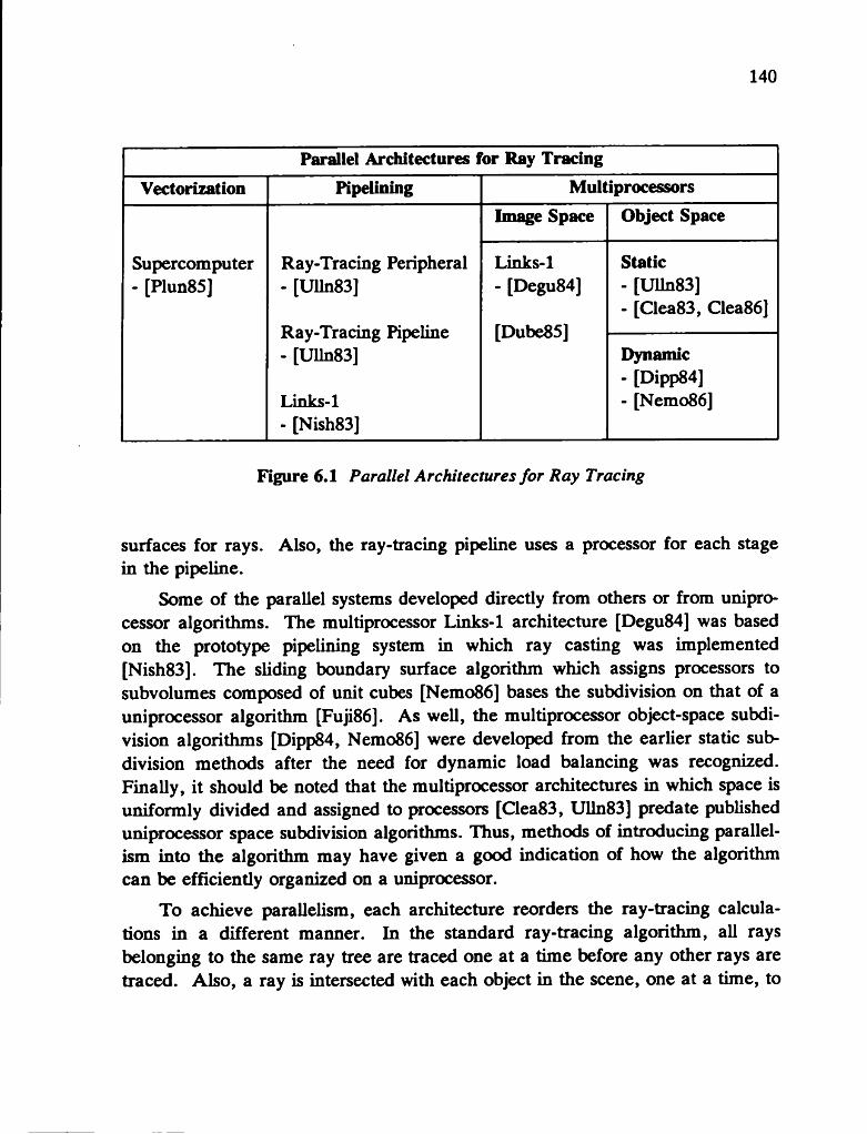
140

Parallel Architectures for Ray TracingVectorization Pipelining Multiprocessors

Supercomputer - [Plun85]

Ray-Tracing Peripheral- [Ulln83]

Ray-Tracing Pipeline- [Ulln83]

Links-1- [Nish83]

Image Space Object Space

Links-1 - [Degu84]

[Dube85]

Static- [Ulln83]- [Clea83, Clea86]

Dynamic- [Dipp84]- [Nemo86]

Figure 6.1 Parallel Architectures for Ray Tracing

surfaces for rays. Also, the ray-tracing pipeline uses a processor for each stage in the pipeline.

Some of the parallel systems developed directly from others or from unipro­cessor algorithms. The multiprocessor Links-1 architecture [Degu84] was based on the prototype pipelining system in which ray casting was implemented [Nish83]. The sliding boundary surface algorithm which assigns processors to subvolumes composed of unit cubes [Nemo86] bases the subdivision on that of a uniprocessor algorithm [Fuji86]. As well, the multiprocessor object-space subdi­vision algorithms [Dipp84, Nemo86] were developed from the earlier static sub­division methods after the need for dynamic load balancing was recognized. Finally, it should be noted that the multiprocessor architectures in which space is uniformly divided and assigned to processors [Clea83, Ulln83] predate published uniprocessor space subdivision algorithms. Thus, methods of introducing parallel­ism into the algorithm may have given a good indication of how the algorithm can be efficiently organized on a uniprocessor.

To achieve parallelism, each architecture reorders the ray-tracing calcula­tions in a different manner. In the standard ray-tracing algorithm, all rays belonging to the same ray tree are traced one at a time before any other rays are traced. Also, a ray is intersected with each object in the scene, one at a time, to

141

determine the closest intersection.In vectorization, parallelism results from intersecting many rays with an

object simultaneously in a single vector operation. To determine visible surfaces for a group of rays, the group is tested for intersection with each object in the scene, one object at a time. As well, part of the parallelism results from having two processors, the scalar processor and the vector processor operating con­currently. Within the vector processor, intersection tests proceed as in a unipro­cessor algorithm, with the difference that many rays are tested for intersection with an object simultaneously. In the host processor, the computations are com­pletely reordered because many primary rays from different pixels are active at the same time. Thus, the ray-tracing algorithm is at a different stage for each primary ray. Shading calculations and the generation of secondary rays are per­formed when intersection results are available for each active ray.

For the ray-tracing peripheral, similar concurrency is achieved between the host computer and the peripheral. The host performs the necessary parts of the ray-tracing algorithm for any rays whose intersection tests have been completed by the peripheral. Within the peripheral, the usual order of the intersection­testing algorithm is used, where a single ray is tested for intersection with objects in the scene, one object at a time. Parallelism is achieved by passing all objects to be intersected through the stages of fetching an object, testing for intersection with the ray, and saving the closest intersection result. Also, within the intersec­tion stage, pipelining allows intersection calculations for different objects to be at different stages.

Once again, concurrency is allowed between the host and the ray-tracing pipeline just as it was in the vector machine and the ray-tracing peripheral. No restrictions are made on the order in which rays are processed and the shading of pixels completed. However, the ray-tracing pipeline reorders the intersection algorithm. In the standard algorithm, a ray is tested for intersection with each object, one object at a time, to determine the visible surface. Because one pro­cessor is assigned to each object, the result is that a single object is tested for intersection with each ray, one ray at a time. Rays are streamed past objects rather than streaming objects past rays. The parallelism introduced allows all objects to be tested for intersection with a single ray simultaneously.

Multiprocessor systems also reorder the standard algorithm to some extent. When the algorithm is divided so that a different region of image space is assigned to each processor, parallelism is achieved because different parts of the

142

image can be rendered simultaneously. Therefore, this design does not really reorder the computations of the algorithm but allows many processors to perform the entire algorithm in parallel. For multiprocessor systems in which a region of object space is assigned to each processor, the computations are reordered. Parallelism is incorporated by allowing many rays to be active at the same time, so that each processor can be intersecting a ray with objects simultaneously. Now, computations are ordered like those in the ray-tracing pipeline where rays are streamed past a fixed set of objects.

While many parallel architectures have been proposed for ray tracing, very few have actually been implemented because certain aspects of the paralleliza­tion limit the efficiency of the system. Of all architectures designed, only two have actually been implemented. The vectorized ray-tracing algorithm for Con­structive Solid Geometry runs on a supercomputer and the multiprocessor Links-1 system is a production ray-tracing system. In the other designs, the effi­ciency is often limited by overhead or by physical considerations for building the system. However, in very few of the architecture designs are these considera­tions addressed.

With vectorization, there is additional overhead in managing the queues of rays and keeping track of the calculations for all pixels. Also, memory require­ments for the queues of rays and intersection results are high. Finally, the size of the ray queue must be finely tuned so that the vector calculation is efficient while still maximizing the utilization of the two processors.

In the pipelined architectures, efficiency is limited by the length of each stage in the pipeline. When stages are of different lengths, the pipeline will be as slow as the slowest stage. In the ray-tracing peripheral, the intersection stage is likely to be the bottleneck in the pipeline. If this stage is extremely long, the only concurrency will be that between the host and the peripheral. This is also true of the ray-tracing pipeline, in which all objects are tested for intersection with a ray simultaneously. If some stages require different times to complete, the pipeline will be as slow as the slowest intersection operation.

With the two types of multiprocessor systems, different factors constrain the physical construction of the architectures, including the amount of memory required and available on each processor as well as communication requirements and overhead. In these systems, methods of load balancing are necessary to ensure that processors are evenly loaded and not idle for significant periods of time.

143

For image-space subdivision, the most critical requirement is memory because each processor needs access to the entire scene description. A shared memory solution is not desirable because of contention among the processors for memory access. However, placing the descriptions in local memory on all pro­cessors requires a lot of memory, greatly increasing the system cost. A mul­tiprocessor system assigned to regions of object space does not have the same memory requirements because object descriptions are distributed over the entire array of processors. Thus, less total memory is required.

Load balancing is necessary for multiprocessor ray-tracing systems if the expected acceleration of the algorithm is to be approached. In image-space sub­division, load balancing is very simple because it is performed statically. How­ever, load balancing is a costly proposition for object-space subdivision because loads of processors change often during ray tracing, requiring that dynamic load balancing be used. This introduces a significant amount of overhead because changing the shapes of the subvolumes and redistributing objects among the pro­cessors are costly operations that must be performed frequently.

In addition to efficiency considerations, each architecture should be able to implement an algorithm in which certain important features and acceleration techniques that have been incorporated into uniprocessor ray tracing are included. Unfortunately, most architectures are designed to execute only a very basic ray-tracing algorithm. Often, the way in which parallelism is introduced precludes the implementation of these features and acceleration methods. For systems without these acceleration techniques, the acceleration observed will not be as great as in systems that can incorporate these methods. Once again, few of these issues have been addressed in the proposals.

Of the features and acceleration techniques developed for uniprocessor ray tracing, a subset has been selected as being important to implement on a parallel architecture. The system should not limit the number of primitive types used to describe the scene. As well, fractal surfaces and primitives with iterative inter­section tests should be included. To add visual complexity to the scene, each of the primitives should be able to be texture- or bump-mapped. Antialiasing by using either uniform or stochastic sampling should be used to produce realistic images with few artifacts. Finally, distributed ray tracing, to model the many blurred phenomena, should be incorporated.

144

Bounding volumes are important for reducing the complexity of the intersec­tion tests. As well, methods of structuring the scene with either object hierar­chies or volume subdivision will greatly reduce the ray tracing time by culling many objects from the set to be tested for intersection with a ray. Tree-depth control to reduce the number of rays traced should also be used. As well, reduc­ing the number of shadow rays created and using a light buffer to restrict the number of objects tested for intersection with the shadow rays are important.

Finally, animation for generating sequences of frames must be considered. This animation is discussed in three categories. The first is camera animation in which only the viewpoint moves between successive frames. The second is object animation, in which objects can change positions between frames. The third is motion blur, modeled by distributed ray tracing, in which objects move during the time of the frame. For each type of animation, restrictions exist for ray trac­ing multiple frames simultaneously.

The table in Figure 6.2 summarizes the features, acceleration techniques, and types of animation that can be implemented by each of the parallel architec­tures.

This table shows that only the multiprocessor architectures can implement the majority of features and acceleration techniques developed for uniprocessor ray tracing. All other architectures have some limitations on the number of features which can be implemented. Vectorization and the ray-tracing pipeline, for which scene structuring cannot be used easily, will always perform much additional work because all objects in the scene must be intersected with each ray in order to achieve the parallelism. However, the tradeoff may still be worthwhile. In vectorization, scene structuring can be implemented, but the overhead may reduce its effectiveness.

Describing a scene with multiple primitives or those with iterative intersec­tions tests presents a problem for the pipelined architectures. Different primitive types have intersection tests requiring different lengths of time to complete. Both architectures rely on using a single primitive type to incorporate pipelining. Therefore, before either the peripheral or the pipeline become feasible, multiple primitive types would have to be included. In the ray-tracing peripheral, this could mean building pipelined circuitry for all intersection algorithms or using bounding volumes. In the ray-tracing pipeline, a method of dividing different intersections tests into a series of identical actions could be one solution. As well, fractal surfaces are very difficult to ray-trace if the surface must be fully

145

Features and Acceleration TechniquesVector

MachineR.T.

PeripheralR.T.

PipelineImageSpace

ObjectSpace

Multiple primitives Y 9• N Y YIterative primitives 9• N N Y YFractal surfaces 9• N N Y YTexture mapping Y Y Y Y YUniform sampling Y Y Y Y YStochastic sampling Y Y Y Y YDistributed R.T. Y Y Y Y YBounding volumes 9• Y N Y YStructuring 9• Y N Y YDepth control Y Y Y Y YNo shadow ray Y Y Y Y YLight Buffer N Y N Y NCamera animation Y Y Y Y YObject animation Y Y Y Y YMotion blur N Y Y Y Y

(Y) - a technique or feature can be implemented (N) - implementation is infeasible or impossible (?) - implementation is possible but not efficient

Figure 6.2 Features and Acceleration Techniques

146

instantiated before ray tracing begins, as is the case for vectorization and the two pipelined architectures.

Motion blur produced by distributed ray tracing cannot be modeled with vectorization because rays in the queue would occur at different times. Since the coordinates of each object are different for each ray, it would not be possible to perform the intersection as a vector operation unless only those rays occurring at the same time were intersected as a group. Finding a suitable group could be difficult and the reduced number of rays in the vector would decrease the effi­ciency of the processor.

In both types of multiprocessor systems, random numbers used to generate fractal surfaces must be chosen carefully to ensure that the same surface is gen­erated by each processor. Each processor must use the same code and table of random numbers to generate each fractal surface. As well, object-space subdivi­sion will have to handle the case where a fractal surface spans multiple subvo­lumes. In this case, each processor through which part of the surface passes must be able to generate the entire surface, although only intersections in its own subvolume are considered.

In distributed ray tracing, jittering in additional dimensions by accessing a permutation table will also have to be done with care. In many of the systems including vectorization, pipelining, and object-space subdivision multiprocessing, many rays from different pixels can be active at the same time. To ensure that the correct permutation in the permutation table is accessed, the index must also be a function of the pixel number. As well, in object-space subdivision multipro­cessing, all processors must have an identical copy of the permutation table so that rays can be jittered properly.

While various parallel architectures have been proposed for ray tracing, few have been implemented because practical considerations limit the efficiency of the system. In each design, the introduction of parallelism should accelerate the computations but very often this theoretical acceleration will not be realized. As well, the introduction of parallelism often restricts the inclusion of the features and acceleration techniques previously incorporated in uniprocessor ray tracers. Even in the multiprocessor systems that can implement the majority of these features and acceleration techniques, the systems are limited by other con­straints. In the image-space subdivision method, the extensive memory require­ments are a problem. In the object-space subdivision method, dynamic load balancing, necessary to ensure that processors are equally loaded, greatly

147

increases the overhead for the system. Thus, dividing the problem in object space will not be feasible until simpler load-balancing algorithms are developed.

Unfortunately, few of these problems have been addressed in any of the designs.

Therefore, although ray tracing produces extremely realistic images, the computational expense of the technique has limited its use. In a single processor system, what may be needed is a hybrid rendering method in which ray tracing is used only to render the complicated pixels of the image. However, such a solution requires the ability to identify those areas of the image for which ray tracing is needed before run time. While various parallel architectures have been designed to introduce parallelism into the algorithm, these methods are currently still in the research stage. Many of the problems that have been identified must be addressed before such architectures can be used to implement a production ray-tracing system.

B ibliography

[Aman87][Appe68]

[Arvo86]

[Barr84]

[Barr86]

[Blin76]

[Blin78]

[Bom59]

[Aman84]

[Bouv85]

John Amanatides, “Ray Tracing with Cones” , Proceedings of SIG- GRAPH ’84 (Minneapolis, Minnesota, July 23-27, 1984), in Com­puter Graphics, 18(3) July 1984, pp. 129-135.John Amanatides, personal communication, January 17, 1987.Arthur Appel, “Some Techniques for Shading Machine Renderings of Solids” , AFIPS 1968 Spring Joint Computer Conference, vol. 32, pp. 37-45, 1968.James Arvo, “Backward Ray Tracing” , unpublished course notes, Developments in Ray Tracing (SIGGRAPH ’86 Course Notes #12, Dallas, Texas, August 18-22, 1986).Alan H. Barr, “Global and Local Deformations of Solid Objects” , Proceedings of SIGGRAPH ’84 (Minneapolis, Minnesota, July 23-27, 1984), in Computer Graphics, 18(3) July 1984, pp. 21-30.Alan H. Barr, “Ray Tracing Deformed Surfaces” , Proceedings of SIGGRAPH ’86 (Dallas, Texas, August 18-22, 1986), in Computer Graphics, 20(4) August 1986, pp. 287-296.James F. Blinn and Martin E. Newell, “Texture and Reflection in Computer Generated Images” , Communications of the ACM, 19(10) October 1976, pp. 542-547.James F. Blinn, “Simulation of Wrinkled Surfaces” , Proceedings of SIGGRAPH ’78 (Atlanta, Georgia, August 23-25, 1978), in Com­puter Graphics, 12(3) August 1978, pp. 286-292.Max Bom and Emil Wolf, Principles of Optics, Pergamon Press Ltd., London, 1959.Christian Bouville, “Bounding Ellipsoids for Ray-Fractal Intersec­tion” , Proceedings of SIGGRAPH ’85 (San Francisco, California, July 22-26, 1985), in Computer Graphics, 19(3) July 1985, pp. 45-52.

148

149

[Catm80]

[Catm84]

[Clar82]

[Clea83]

[Clea86]

[Cohe85]

[Cohe86]

[Carp84]

[Cook82]

Loren Carpenter, “The A-buffer, an Antialiased Hidden Surface Method” , Proceedings of SIGGRAPH ’84 (Minneapolis, Minnesota, July 23-27, 1984), in Computer Graphics, 18(3) July 1984, pp. 103- 108.Ed Catmull and Alvy Ray Smith, “3-D Transformations of Images in Scanline Order” , Proceedings of SIGGRAPH ’80 (Seattle, Wash­ington, July 14-18, 1980), in Computer Graphics, 14(3) July 1980, pp. 279-285.Edwin Catmull, “An Analytic Visible Surface Algorithm for In­dependent Pixel Processing” , Proceedings of SIGGRAPH ’84 (Min­neapolis, Minnesota, July 23-27, 1984), in Computer Graphics, 18(3) July 1984, pp. 109-115.James H. Clark, “The Geometry Engine: A VLSI Geometry System for Graphics” , Proceedings of SIGGRAPH ’82 (Boston, Mas­sachusetts, July 26-30, 1982), in Computer Graphics, 16(3) July 1982, pp. 127-133.John G. Cleary, Brian Wyvill, Reddy Vatti, and Graham M. Birtwistle, “Design and Analysis of a Parallel Ray Tracing Com­puter” , in Proceedings of Graphics Interface ’83 (Edmonton, Alberta, May 9-13, 1983), pp. 33-34.John G. Cleary, Brian Wyvill, Graham M. Birtwistle, and Reddy Vatti, “Multiprocessor Ray Tracing” , Computer Graphics Forum, 5(1) March 1986, pp. 3-12.Michael F. Cohen and Donald P. Greenberg, “The Hemi-Cube: A Radiosity Solution for Complex Environments” , Proceedings of SIG­GRAPH ’85 (San Francisco, California, July 22-26, 1985), in Com­puter Graphics, 19(3) July 1985, pp. 31-40.Michael F. Cohen, Donald P. Greenberg, David S. Immel, and Phi­lip J. Brock, “An Efficient Radiosity Approach for Realistic Image Synthesis” , IEEE Computer Graphics and Applications, 6(3) March 1986, pp. 26-35.Robert L. Cook and Kenneth E. Torrance, “A Reflectance Model for Computer Graphics” , ACM Transactions on Graphics”, 1(1) Janu­ary 1982, pp. 7-24.

150

[Cook86a]

[Cook86b]

[Crow77]

[Crow81]

[Degu84]

[Dipp85]

[Dipp84]

[Dube85]

[Cook84]

[Dube86]

Robert L. Cook, Thomas Porter, and Loren Carpenter, “Distributed Ray Tracing” , Proceedings of SIGGRAPH ’84 (Minneapolis, Min­nesota, July 23-27, 1984), in Computer Graphics, 18(3) July 1984, pp. 137-145.Robert L. Cook, “Stochastic Sampling in Computer Graphics” , ACM Transactions on Graphics, 5(1) January 1986, pp. 51-72.Robert L. Cook, “Practical Aspects of Distributed Ray Tracing” , unpublished course notes, Developments in Ray Tracing (SIG­GRAPH *86 Course Notes #12, Dallas, Texas, August 18-22, 1986).Franklin C. Crow, “The Aliasing Problem in Computer-Generated Shaded Images” , Communications of the ACM, 20(11) November 1977, pp. 799-805.Franklin C. Crow, “A Comparison of Antialiasing Techniques” , Computer Graphics and Applications, 1(1) January 1981, pp. 40-48.Hiroshi Deguchi, Hitoshi Nishimura, Hiroshi Yoshimura, Torn Kawata, Isao Shirakawa, and Koichi Omura, “A Parallel Processing Scheme for Three-dimensional Image Generation” , in Conference Proceedings International Symposium on Circuits and Systems (ISCAS •84), pp. 1285-1288, 1984.Mark A. Z. Dipp6 and Erling Henry Wold, “Antialiasing Through Stochastic Sampling” , Proceedings of SIGGRAPH ’85 (San Fran­cisco, California, July 22-26, 1985), in Computer Graphics, 19(3) July 1985, pp. 69-78.Mark E. Dipp6 and John Swensen, “An Adaptive Subdivision Algo­rithm and Parallel Architecture for Realistic Image Synthesis” , Proceedings of SIGGRAPH ’84 (Minneapolis, Minnesota, July 23-27, 1984), in Computer Graphics, 18(3) July 1984, pp. 149-158.Martin W. Dubetz, Ray Tracing Algorithms for Computer Graphics, PhD thesis, University of Alberta, 1985.Martin Dubetz and John Tartar, “An Object/Volume Hierarchy for Raytracing” , in preparation, Dept, of Computer Science, University of Alberta, 1986.

151

[Floy75]

[Fole83]

[Four82]

[Fuch81]

[Fuch85]

[Fuch80]

[Fuji86]

[Fuss82]

[Fium83] Eugene Fiume, Alain Fournier, and Larry Rudolph, “A Parallel Scan Conversion Algorithm with Anti-Aliasing for a General- Purpose Ultracomputer” , Proceedings of SIGGRAPH ’83 (Detroit, Michigan, July 25-29, 1983), in Computer Graphics, 17(3) July 1983, pp. 141-150.R. Floyd and L. Steinberg, “An Adaptive Algorithm for Spatial Grey Scale” , Society for Information Display, 1975, p. 36-37.James D. Foley and Andries van Dam, Fundamentals of Interactive Computer Graphics (Corrected 1st Edition), 1983.Alain Fournier, Don Fussell, and Loren Carpenter, “Computer Rendering of Stochastic Models” , Communications of the ACM, 25(6) June 1982, pp. 371-384.Henry Fuchs and John Poulton, “Pixel-Planes: A VLSI-Oriented Design for a Raster Graphics Engine” , VLSI Design, 2(3) Third Quarter 1981, pp. 20-28.Henry Fuchs, Jack Goldfeather, Jeff P. Hultquist, Susan Spach, John D. Austin, Frederick P. Brooks Jr., John G. Eyles, and John Poulton, “Fast Spheres, Shadows, Textures, Transparencies, and Im­age Enhancements in Pixel-Planes” , Proceedings of SIGGRAPH ’85 (San Francisco, California, July 22-26, 1985), in Computer Graphics, 19(3) July 1985, pp. 111-120.Henry Fuchs, Zvi M. Kedem, and Bruce F. Naylor, “On Visible Surface Generation by A Priori Tree Structures” , Proceedings of SIGGRAPH ’80 (Seattle, Washington, July 14-18, 1980), in Com­puter Graphics, 14(3) July 1980, pp. 124-133.Akira Fujimoto, Takayuki Tanaka, and Kansei Iwata, “ARTS: Ac­celerated Ray-Tracing System” , IEEE Computer Graphics and Appli­cations, 6(4) April 1986, pp. 16-26.Donald Fussell and Bharat Deep Rathi, “A VLSI-Oriented Archi­tecture for Real-Time Raster Display of Shaded Polygons” , Proceed­ings of Graphics Interface ’82 (Toronto, Ontario, May 17-21, 1982), pp. 373-380.

152

[Gold86]

[Gold71]

[Gora84]

[Glas84]

[Hain86]

[HaU83]

[Hama84]

[Hanr83]

[Hanr86]

[Heck84]

Andrew S. Glassner, “Space Subdivision for Fast Ray Tracing” , IEEE Computer Graphics and Applications, 4(10) October 1984, pp. 15-22.Jack Goldfeather, Jeff P. M. Hultquist, and Henry Fuchs, “Fast Constructive Solid Geometry Display in the Pixel-Powers Graphics System” , Proceedings of SIGGRAPH ’86 (Dallas, Texas, August 18-22, 1986), in Computer Graphics, 20(4) August 1986, pp. 107- 116.Robert A. Goldstein and Roger Nagel, “3-D Visual Simulation” , Simulation, 16(1) January 1971, pp. 25-31.Cindy M. Goral, Kenneth E. Torrance, Donald P. Greenberg, and Bennett Battaile, “Modeling the Interaction of Light Between Dif­fuse Surfaces” , Proceedings of SIGGRAPH ’84 (Minneapolis, Min­nesota, July 23-27, 1984), in Computer Graphics, 18(3) July 1984, pp. 213-222.Eric A. Haines and Donald P. Greenberg, “The Light Buffer: A Shadow-Testing Accelerator” , IEEE Computer Graphics and Applica­tions, 6(9) September 1986, pp. 6-16.Roy A. Hall and Donald P. Greenberg, “A Testbed for Realistic Image Synthesis” , IEEE Computer Graphics and Applications, 3(8) November 1983, pp. 10-20.V. Carl Hamacher, Zvonko G. Vranesic, and Safwat G. Zaky, Computer Organization (Second Edition), 1984.Pat Hanrahan, “Ray Tracing Algebraic Surfaces, Proceedings of SIGGRAPH ’83 (Detroit, Michigan, July 25-29, 1983), in Computer Graphics, 17(3) July 1983, pp. 83-90.Pat Hanrahan, “Using Caching and Breadth-First Search to Speed Up Ray-Tracing” (extended abstract), Proceedings Graphics Inter­face ’86 (Vancouver, B.C., May 26-30, 1986), pp. 56-61, May 1986.Paul S. Heckbert and Pat Hanrahan, “Beam Tracing Polygonal Ob­jects” , Proceedings of SIGGRAPH ’84 (Minneapolis, Minnesota, July 23-27, 1984), in Computer Graphics, 18(3) July 1984, pp. 119- 127.

153

[Hunt75]

[Hwan84]

[Imme86]

[Inak86]

[Joy86]

[Kaji82]

[Kaji83a]

[Kaji83b]

[Kaji84]

Richard S. Hunter, The Measurement of Appearance, John Wiley and Sons, Inc., New York, 1975.Kai Hwang and Fay6 A. Briggs, Computer Architecture and Parallel Processing, 1984.David S. Immel, Michael F. Cohen, and Donald P. Greenberg, “A Radiosity Method for Non-Diffuse Environments” , Proceedings of SIGGRAPH ’86 (Dallas, Texas, August 18-22, 1986), in Computer Graphics, 20(4) August 1986, pp. 133-142.Masa Inakage, ‘‘Reflection and Refraction Model for Ray Tracing” , unpublished course notes, Developments in Ray Tracing (SIG­GRAPH ’86 Course Notes #12, Dallas, Texas, August 18-22, 1986).Kenneth I. Joy and Murthy N. Bhetanabhotla, “Ray Tracing Parametric Surface Patches Utilizing Numerical Techniques and Ray Coherence” , Proceedings of SIGGRAPH ’86 (Dallas, Texas, Au­gust 18-22, 1986), in Computer Graphics, 20(4) August 1986, pp. 279-284.James T. Kajiya, “Ray Tracing Parametric Patches” , Proceedings of SIGGRAPH ’82 (Boston, Massachusetts, July 26-30, 1982), in Com­puter Graphics, 16(3) July 1982, pp. 245-254.James T. Kajiya, “New Techniques for Ray Tracing Procedurally Defined Objects” , Proceedings of SIGGRAPH ’83 (Detroit, Michi­gan, July 25-29, 1983), in Computer Graphics, 17(3) July 1983, pp. 91-102.James T. Kajiya, “SIGGRAPH ’83 Tutorial on Ray Tracing” , un­published course notes, State of the Art in Image Synthesis (SIG­GRAPH ’83 Course Notes #10, Detroit, Michigan, July 25-29, 1983).James T. Kajiya and Brian P. Von Herzen, “Ray Tracing Volume Densities” , Proceedings of SIGGRAPH ’84 (Minneapolis, Min­nesota, July 23-27, 1984), in Computer Graphics, 18(3) July 1984, pp. 165-174.

154

[Kaji86]

[Kapl85]

[Kay86]

[King86]

[Kore83]

[Lane80]

[Lee85]

[Kaji85]

[Max85]

James T. Kajiya, “Anisotropic Reflection Models” , Proceedings of SIGGRAPH ’85 (San Francisco, California, July 22-26, 1985), in Computer Graphics, 19(3) July 1985, pp. 15-21.James T. Kajiya, “The Rendering Equation” , Proceedings of SIG­GRAPH ’86 (Dallas, Texas, August 18-22, 1986), in Computer Graphics, 20(3) August 1986, pp. 143-150.Michael R. Kaplan, “Space-Tracing, A Constant Time Ray- Tracer” , unpublished course notes, State of the Art in Image Syn­thesis (SIGGRAPH ’85 Course Notes #11, San Francisco, Califor­nia, July 22-26, 1985).Timothy L. Kay and James T. Kajiya, “Ray Tracing Complex Scenes” , Proceedings of SIGGRAPH ’86 (Dallas, Texas, August 18-22, 1986), in Computer Graphics, (20)4 August 1986, pp. 269- 276.Stewart Kingdon, “Speeding Up Ray-Scene Intersections” , Master’s thesis, University of Waterloo, 1986.Jonathan Korein and Norman Badler, “Temporal Antialiasing in Computer Generated Animation” , Proceedings of SIGGRAPH ’83 (Detroit, Michigan, July 25-29, 1983), in Computer Graphics, 17(3) July 1983, pp. 377-388.Jeffrey M. Lane, Loren C. Carpenter, Turner Whitted, and James F. Blinn, “Scan Line Methods for Displaying Parametrically Defined Surfaces” , Communications of the ACM, 23(1) January 1980, pp. 23-34.Mark E. Lee, Richard A. Redner, and Samuel P. Uselton, “Statisti­cally Optimized Sampling for Distributed Ray Tracing” , Proceedings of SIGGRAPH ’85 (San Francisco, California, July 22-26, 1985), in Computer Graphics, 19(3) July 1985, pp. 61-67.Nelson L. Max and Douglas M. Lemer, “A Two-and-a-Half-D Mo­tion Blur Algorithm”, Proceedings of SIGGRAPH ’85 (San Fran­cisco, California, July 22-26, 1985), in Computer Graphics, 19(3) July 1985, pp. 85-93.

155

[Nemo86]

[Nish83]

[Nish85]

[Oppe86]

[Plun85]

[Potm82]

[Potm83]

[Mitc87]

[Reev83]

Don P. Mitchell, “Generating Antialiased Imaged at Low Sampling Densities” , Proceedings of SIGGRAPH ’87 (Anaheim, California, July 27-31, 1987), in Computer Graphics, 21(4) July 1987, pp. 65-72.Keiji Nemoto and Takao Omachi, “An Adaptive Subdivision by Sliding Boundary Surfaces for Fast Ray Tracing” , Proceedings of Graphics Interface ’86 (Vancouver, B.C., May 26-30, 1986), pp. 43-48, May 1986.Hitoshi Nishimura, Hiroshi Ohno, Torn Kawata, Isao Shirakawa, and Koichi Omura, “Links-1: A Parallel Pipelined Multimicrocom­puter System for Image Creation” , in Conference Proceedings of the 10th Annual International Symposium on Computer Architecture, SIGARCH, pp. 387-394, 1983.Tomoyuki Nishita and Eihachiro Nakamae, “Continuous Tone Representation of Three-Dimensional Objects Taking Account of Shadows and Interreflection” , Proceedings of SIGGRAPH ’85 (San Francisco, California, July 22-26, 1985), in Computer Graphics, 19(3) July 1985, pp. 23-30.Peter E. Oppenheimer, “Real Time Design and Animation of Frac­tal Plants and Trees”, Proceedings of SIGGRAPH ’86 (Dallas, Texas, August 18-22, 1986), in Computer Graphics, 20(4) August 1986, pp. 55-64.David J. Plunkett and Michael J. Bailey, “The Vectorization of a Ray Tracing Algorithm for Improved Execution Speed” , IEEE Com­puter Graphics and Applications, 5(8) August 1985, pp. 52-60.Michael Potmesil and Indranil Chakravarty, “Synthetic Image Gen­eration with a Lens and Aperture Camera Model” , ACM Transac­tions on Graphics, 1(2) April 1982, pp. 85-108.Michael Potmesil and Indranil Chakravarty, “Modeling Motion Blur in Computer Generated Images” , Proceedings of SIGGRAPH ’83 (Detroit, Michigan, July 25-29, 1983), in Computer Graphics, 17(3) July 1983, pp. 389-399.William T. Reeves, “Particle Systems - A Technique for Modeling a Class of Fuzzy Objects” , ACM Transactions on Graphics, 2(2) April 1983, pp. 91-108.

156

[Rubi80]

[Rush87]

[Sede84]

[Sieg81]

[Smit84]

[Snyd87]

[Spar78]

[Spee85]

[Roth82]

[Suth74]

Scott D. Roth, “Ray Casting for Modeling Solids’’, Computer Graph­ics and Image Processing, 18(2) February 1982, pp. 109-144.Steven M. Rubin and Turner Whitted, “A 3-Dimensional Represen­tation for Fast Rendering of Complex Scenes” , Proceedings of SIG- GRAPH ’80 (Seattle, Washington, July 14-18, 1980), in Computer Graphics, 14(3) July 1980, pp. 110-116.Holly E. Rushmeier and Kenneth E. Torrance, “The Zonal Method for Calculating Light Intensities in the Presence of a Participating Medium”, Proceedings of SIGGRAPH ’87 (Anaheim, California, July 27-31, 1987), in Computer Graphics, 21(4) July 1987, pp. 293- 302.Thomas W. Sederberg and David C. Anderson, “Ray Tracing of Steiner Patches” , Proceedings of SIGGRAPH ’84 (Minneapolis, Minnesota, July 23-27, 1984), in Computer Graphics, 18(3) July 1984, pp. 159-164.Robert Siegel and John R. Howell, Thermal Radiation Heat Transfer (Second Edition), Hemisphere Publishing Corporation, Washington, 1981.Alvy Ray Smith, “Plants, Fractals, and Formal Languages” , Proceedings of SIGGRAPH ’84 (Minneapolis, Minnesota, July 23-27, 1984), in Computer Graphics, 18(3) July 1984, pp. 1-10.John M. Snyder and Alan H. Barr, “Ray Tracing Complex Models Containing Surface Tessellations” , Proceedings of SIGGRAPH ’87 (Anaheim, California, July 27-31, 1987), in Computer Graphics, (21)4 July 1987, pp. 119-128.E. M. Sparrow and R. D. Cess, Radiation Heat Transfer, Hemi­sphere Publishing Corporation, Washington, 1978.L. Richard Speer, Tony D. DeRose, and Brian A. Barsky, “A Theoretical and Empirical Analysis of Coherent Ray-Tracing” , Proceedings of Graphics Interface ’85 (Montreal, Que., May 27-31, 1985), pp. 1-8, May 1985.Ivan E. Sutherland, Robert F. Sproull, and Robert A. Schumacker, “A Characterization of Ten Hidden Surface Algorithms” , ACM Computing Surveys, 6(1) March 1974, pp. 1-55.

157

[Swee86]

[Torb87]

[Toth85]

[Ulln83]

[Wall87]

[Wegh84]

[Wein81]

[Whel86]

[Swee84]

[Whit80]

Michael A. J. Sweeney, “The Waterloo Ray Tracing Package” , Master’s thesis, University of Waterloo, 1984.Michael A. J. Sweeney and Richard H. Bartels, “Ray-Tracing Free-Form B-Spline Surfaces” , IEEE Computer Graphics and Applica­tions, 6(2) February 1986, pp. 41-49.John G. Torborg, “A Parallel Processor Architecture for Graphics Arithmetic Operations” , Proceedings of SIGGRAPH ’87 (Anaheim, California, July 27-31, 1987), in Computer Graphics, (21)4 July 1987, pp. 197-204.Daniel L. Toth, “On Ray Tracing Parametric Patches” , Proceedings of SIGGRAPH ’85 (San Francisco, California, July 22-26, 1985), in Computer Graphics, 19(3) July 1985, pp. 171-179.Michael K. Ullner, Parallel Machines for Computer Graphics, PhD thesis, California Institute of Technology, 1983.John R. Wallace, Michael F. Cohen, and Donald P. Greenberg, “A Two-Pass Solution to the Rendering Equation: A Synthesis of Ray Tracing and Radiosity Methods” , Proceedings of SIGGRAPH ’87 (Anaheim, California, July 27-31, 1987), in Computer Graphics, 21(4) July 1987, pp. 311-320.Hank Weghorst, Gary Hooper, and Donald P. Greenberg, “Im­proved Computational Methods for Ray Tracing” , ACM Transactions on Graphics, 3(1) January 1984, pp. 52-69.Richard Weinberg, “Parallel Processing Image Synthesis and Anti- Aliasing” , Proceedings of SIGGRAPH ’81 (Dallas, Texas, August 3-7, 1981), in Computer Graphics, 15(3) August 1981, pp. 55-62.Daniel S. Whelan, ANIMAC: A Multiprocessor Architecture for Real- Time Computer Animation, PhD thesis, California Institute of Tech­nology, 1986.Turner Whitted, “An Improved Illumination Model for Shaded Display” , Communications of the ACM, 23(6) June 1980, pp. 343- 349.

158

[WU178]

[Wyvi86]

Lance Williams, “Casting Curved Shadows on Curved Surfaces” , Proceedings of SIGGRAPH ’78 (Atlanta, Georgia, August 23-25, 1978), in Computer Graphics, 12(3) August 1978, pp. 270-274.Geoff Wyvill, Tosiyasu L. Kunii, and Yasuto Shirai, “Space Divi­sion for Ray Tracing in CSG” , IEEE Computer Graphics and Applica­tions, 6(4) April 1986, pp. 28-34.

G lossary

3D-DDAa Three Dimensional Digital Differential Analyzer used to determine the unit cubes intersected by a ray. As such, it is the extension of a digital differential analyzer that determines the pixels to be illuminated when scan-converting a line.

Adaptive Samplinga sampling method that generates additional primary rays for pixels where there is evidence of marked intensity change in the image.

Adaptive Subdivisiona space subdivision method in which only cells containing more than a maximum number of primitives are recursively subdivided.

Beama group of rays traced as a unit, formed by sweeping a polygon through space.

Beam Treea tree in which branches represent beams and nodes contain exact inter­section results for all surfaces intersected.

Beam Tracingan algorithm that traces beams instead of single rays, forming a beam tree. This produces a resolution-independent solution for the scene which can be rendered with scan-line methods.

Boundary Surfaceone of two boundaries of a subvolume with planes perpendicular to the driving axis. In a multiprocessor system assigning subvolumes composed of unit cubes to different processors, this surface can be moved by one cube to redistribute the load.

Bounding Volumea simple volume that completely encloses an object. It is used to simplify intersection tests so that only if a ray strikes the bounding volume is the

159

160

object tested for intersection with the ray.Bounding-Volume Hierarchy

a scene-structuring method that groups nearby objects into a tree of bounding volumes. The bounding volume at each node completely en­closes the bounding volumes of all its children. During traversal, a ray is intersected with the bounding volume at a node. Only if there is an inter­section are any of the child bounding volumes examined.

Bounding Volume in Timea bounding volume that encloses a moving object during the entire time of one frame. It is used in modeling of motion blur to allow rays occur­ring at different instants of time within a frame to be intersected with the same bounding volume. This avoids the costly movement of objects and creation of bounding volumes for each ray traced.

BSP Treea Binary Space Partitioning Tree for space subdivision. Division of a sub­volume into eight equal-sized subvolumes is made by specifying seven slicing nodes, each of which divides space along a different axis.

Cachinguses coherence by saving and reusing previous intersection results. Often, this is done by saving the ray tree from the previous pixel and using the intersection result for the corresponding ray in that tree as an initial ap­proximation for the current point of intersection. A similar method is used for shadow rays. Caching avoids additional intersection testing if the predicted object is intersected.

Causticpattern of different intensities of light caused when light is focussed on a diffuse surface by a transparent object. This term originates in optics, where it refers to a curved surface illuminated by light focussed by a lens.

Colour Bleedinga phenomenon noticed on a diffuse surface that is illuminated by another very close diffuse surface acting as a secondary light source.

Coneformed by grouping many rays emanating from a single point into a cone of light to be traced as a unit.

161

Cone Tracingan algorithm that traces many rays as a unit by grouping them into a cone. Tracing a cone of rays through each pixel replaces tracing multiple primary rays. Antialiasing is performed by recording all surfaces that a cone intersects.

Depth of Fielda phenomenon observed in images produced using a camera with finite lens aperture in which objects in front of or behind the focal point appear blurred.

Diffuse Surfacea dull or matte surface with little or no specular component. Illumination of such a surface is difficult to model with ray tracing.

Distributed Ray Tracingan extension of the ray-tracing algorithm that models a range of blurred phenomena including gloss, translucency, penumbras, depth of field, and motion blur. Ray directions are not determined precisely, but are distri­buted about the usual direction. As well, additional samples are not taken to model each phenomenon, but perturbations are applied to each primary ray generated for the pixel. If done by jittering, the entire range of values for a phenomenon will be sampled.

Driving Axisthe axis along which the number of objects in the scene is the most varied.

Form Factora term specifying the fraction of energy leaving one surface that is in­cident on another and is used in the radiosity method to compute illumi­nation of diffuse surfaces. Although this term was coined for radiosity, these factors originated in radiation heat transfer theory.

Fractal Surfacea procedurally-defined object formed by recursively subdividing a polygon until enough small polygons have been generated to completely describe the surface. In ray tracing, a triangle is most often divided, with the height of each new vertex varied randomly.

162

General Cubea six-sided subvolume whose eight comers can be located anywhere in three-space. A dynamic load balancing algorithm uses this type of subvo­lume to allow shapes of subvolumes to be altered while keeping adjacent subvolumes assigned to connected processors.

Glossa phenomenon in which objects seen in a reflective surface appear blurred. In ray tracing, this effect is produced by sampling about the specular reflection direction.

Image Planean imaginary transparent grid representing the screen onto which the im­age will be projected. It is placed between the viewpoint and the objects of the scene so that rays are generated from the viewpoint through each “pixel” of this grid.

Image-Space Subdivisiona multiprocessor ray-tracing system in which the image is divided into many subimages, with one assigned to each processor, so that many can be ray traced in parallel.

Implicit Surfacea surface whose points are found by solving the equation F (x ,y ,z ) = 0, where F is a function describing the surface. Examples of such surfaces where F is polynomial include spheres, planes, cones, and cylinders.

Jitteringa non-uniform sampling method used to ensure that samples are selected from the entire range of values for a phenomenon. Jittering can sample the pixel area to perform antialiasing by dividing a pixel into subpixels and generating a random sample point in each subpixel. Jittering can also sample other phenomena in distributed ray tracing by dividing the range over which samples are taken into subranges and selecting a ran­dom value within each subrange.

Light Buffera cache created for each light source identifying a subset of objects that must be tested for intersection with a shadow ray. A light buffer is created by projecting the scene onto the faces of a cube centred around each light source. Each entry indicates the objects visible through a grid

163

location for a particular view.

Light Raya ray originating from a light source.

Load Balancinga method of distributing the computations of a problem to multiple proces­sors in such a way that the processors are evenly loaded. Such an algo­rithm is necessary for the system to be efficient. The method can be static or dynamic.

Moiréan aliasing artifact in which regularly-repeating patterns of concentric cir­cles appear as swirled curves in the image.

Motion Blura phenomenon in which the images of fast-moving objects appear blurred. The effect is created by taking samples at different instants of time during a single frame.

Non-uniform Samplinga sampling method in which sample points are not regularly-spaced. This will reduce many aliasing artifacts that may appear in an image.

Nyquist Limitdefined to be half the sampling rate. A regular pattern with a frequency greater than this limit will alias to a pattern of a lower frequency.

Object Hierarchya hierarchy of bounding volumes in which leaf nodes are objects and bounding volumes at interior nodes encompass the bounding volumes of their children. This scene-structuring method reduces the number of ray- object intersection tests by culling objects. Only those subtrees below bounding volumes that a ray intersects are ever expanded.

Object-Space Subdivisiona multiprocessor ray-tracing system in which object space is divided and a subvolume assigned to each processor. Rays entering a subvolume are modeled by messages sent to the processor responsible for the subvolume. Only those objects in this subvolume need to be tested for intersection with the ray.

164

Object-Volume Hierarchya hybrid scene-structuring method combining an object hierarchy with volume subdivision. An object hierarchy is located at the top of the struc­ture with a separate volume hierarchy created (if necessary) for each leaf node of the object hierarchy.

Octreea tree in which each node has eight children. The structure is used to describe adaptive subdivision of object space because division along all three axes produces eight equal-sized subvolumes.

Parametric Surfacea surface whose points must be explicitly generated by means of parametric equations that map a set of parameters to a set of points. If the equation of the parametric surface is polynomial, the ray-surface in­tersection can be solved directly. Otherwise, numerical methods must be used. Steiner patches, bicubic patches, and B-spline surfaces are exam­ples of parametric surfaces.

Path Tracinga ray-tracing method in which only one ray, either a reflected ray or a re­fracted ray, is followed from each intersection point.

Penumbraa fuzzy shadow whose edges show a gradual transition from light to dark, resulting when a light source is partially-obscured by another object. This phenomenon is modeled by distributing rays over the area of the light source.

Permutation Tablea random list of all possible permutations of numbers that map ranges of values describing a phenomenon to a screen-space location on a pixel. This table is used in distributed ray tracing to ensure that there is no correlation among rays sampling different phenomena.

Pipelininga hardware method of achieving parallelism by dividing a task into a series of stages through which many data items must be passed. When the pipeline is full, N stages can process N data items in parallel.

165

Poisson Disk Distributiona non-uniform distribution in which all sample points are separated by some m in im um distance. This is the same as the distribution of photore­ceptors in the human eye.

Primary Light Sourcean object that emits light.

Primary Raya ray generated from the viewpoint through a grid location of the image plane into the scene.

Radiositya method of calculating the exact exchange of illumination between dif­fusely reflecting surfaces using form factors. The method was later ex­tended to handle specular surfaces.

Ray Castingan algorithm similar to ray tracing in which no additional rays are traced from the intersection point on the visible surface.

Ray Coherencea form of coherence where rays from adjacent pixels follow approximately the same path through the scene, striking the same visible objects and generating secondary rays in similar directions.

Ray Tracingan image generation technique that simulates rays of light moving through the scene. This method produces very realistic images with many phenomena including reflections, transparency, shadows, gloss, translu- cency, penumbras, motion blur, and depth of field.

Ray Treea tree associated with each primary ray in which branches represent rays of light and nodes represent objects intersected by the incoming ray.

Reflectivitya surface property that allows light to be reflected from a surface in the mirror direction.

Scene Volumea bounding volume that completely encloses all objects of the scene.

166

Secondary Light Sourcea reflective or transparent object that transports light. Secondary light sources are very important for the illumination of diffuse surfaces.

Shadow Raya ray generated from the intersected point on a surface in the direction of a light source. The point is in shadow if the ray is blocked by any object.

Slabthe region of space bounded by two parallel planes. Three or more non­parallel slabs can be used to form a tight bounding volume.

Stochastic Samplinga Monte Carlo method that generates non-uniform patterns of sample points.

Supersamplingan antialiasing method that generates more than one primary sample ray per pixel and weights the resulting intensities.

Tessellationa method of breaking a surface into many tiny pieces that are usually simpler to ray-trace than the original surface.

Texture Mappinga process that projects a pattern onto a surface to add visual complexity to a scene.

Three Dimensional DDA See 3D-DDA.

Translucencya blurred transparency caused by light scattering as it passes through a translucent surface. This phenomenon is modeled by distributing rays about the direction of refraction.

Transparencya property that allows light to pass directly through a surface, although the rays may be refracted or bent.

Tree-Depth Controlan algorithm that reduces the number of rays traced by limiting the depth of the ray tree. If adaptive depth control is used, no more rays are gen­erated when the maximum contribution to a pixel becomes less than some

167

minimum intensity.Uniform Sampling

a sampling method in which sample points are regularly-spaced, leading to aliasing for sampled patterns above the Nyquist Limit.

Uniform Volume Subdivisiona space-subdivision method where all subvolumes are the same size.

Vectorizationa method that introduces parallelism with a vector machine by performing the same operation on all elements of a vector simultaneously.

Viewpointthe location in object space of the camera or eye. All primary rays emanate from this point.

Visible-Surface Preprocessan algorithm that determines the visible objects for each pixel by project­ing the scene onto the image plane.

Volume Subdivisiona scene-structuring method that divides object space either uniformly or adaptively into subvolumes. Then, only objects in those subvolumes through which the ray passes are tested for intersection with the ray.