“all-in-one”test system modellingand...

“All-in-one” test system modelling andsimulation for multiple instability scenarios

Internal Report

Report # Smarts-Lab-2011-002

April 2011

Principal Investigators:

Ph.D. student Rujiroj LeelarujiDr. Luigi Vanfretti

Affiliation:

KTH Royal Institute of TechnologyElectric Power Systems Department

KTH • Electric Power Systems Division • School of Electrical Engineering • Teknikringen 33 • SE 100 44 Stockholm • Sweden

Dr. Luigi Vanfretti • Tel.: +46-8 790 6625 • [email protected] • www.vanfretti.com

DISCLAIMER OF WARRANTIES AND LIMITATION OF LIABILITIES

THIS DOCUMENT WAS PREPARED BY THE ORGANIZATION(S) NAMED BELOW AS AN ACCOUNT OF

WORK SPONSORED OR COSPONSORED BY KUNGLIGA TEKNISKA HOGSKOLAN (KTH) . NEITHER KTH,

ANY MEMBER OF KTH, ANY COSPONSOR, THE ORGANIZATION(S) BELOW, NOR ANY PERSON ACTING

ON BEHALF OF ANY OF THEM:

(A) MAKES ANY WARRANTY OR REPRESENTATION WHATSOEVER, EXPRESS OR IMPLIED, (I) WITH

RESPECT TO THE USE OF ANY INFORMATION, APPARATUS, METHOD, PROCESS, OR SIMILAR ITEM

DISCLOSED IN THIS DOCUMENT, INCLUDING MERCHANTABILITY AND FITNESS FOR A PARTICULAR

PURPOSE, OR (II) THAT SUCH USE DOES NOT INFRINGE ON OR INTERFERE WITH PRIVATELY OWNED

RIGHTS, INCLUDING ANY PARTY’S INTELLECTUAL PROPERTY, OR (III) THAT THIS DOCUMENT IS

SUITABLE TO ANY PARTICULAR USER’S CIRCUMSTANCE; OR

(B) ASSUMES RESPONSIBILITY FOR ANY DAMAGES OR OTHER LIABILITY WHATSOEVER (INCLUDING

ANY CONSEQUENTIAL DAMAGES, EVEN IF KTH OR ANY KTH REPRESENTATIVE HAS BEEN ADVISED OF

THE POSSIBILITY OF SUCH DAMAGES) RESULTING FROM YOUR SELECTION OR USE OF THIS

DOCUMENT OR ANY INFORMATION, APPARATUS, METHOD, PROCESS, OR SIMILAR ITEM DISCLOSED IN

THIS DOCUMENT.

ORGANIZATIONS THAT PREPARED THIS DOCUMENT:

KUNGLIGA TEKNISKA HOGSKOLAN

ORDERING INFORMATION

Requests for copies of this report should be directed to Dr. Luigi Vanfretti, Teknikringen 33, SE-100 44,

Stockholm, Sweden. Phone: +46 8 790 66 25; Fax: +46 8 790 65 10.

CITING THIS DOCUMENT

Leelaruji, R., and Vanfretti, L. “All-in-one” test system modelling and simulation for multiple instability

scenarios. Internal Report. Stockholm: KTH Royal Institute of Technology. April 2011. Available

on-line:http://www.vanfretti.com

Copyright c© 2010 KTH, Inc. All rights reserved.

2

Contents

1 System Modelling 4

1.1 Excitation System . . . . . . . . . . . . . . . . . . . . . . . . . . . . . . . . . . . 41.2 Overexcitation Limiter (OEL) . . . . . . . . . . . . . . . . . . . . . . . . . . . . . 61.3 Speed-Governing System . . . . . . . . . . . . . . . . . . . . . . . . . . . . . . . . 71.4 Steam Turbine System . . . . . . . . . . . . . . . . . . . . . . . . . . . . . . . . . 81.5 Load Tap Changer (LTC) . . . . . . . . . . . . . . . . . . . . . . . . . . . . . . . 91.6 Load restoration model . . . . . . . . . . . . . . . . . . . . . . . . . . . . . . . . 9

2 Simulation results 11

2.1 Transient (angle) instability . . . . . . . . . . . . . . . . . . . . . . . . . . . . . . 112.2 Frequency instability . . . . . . . . . . . . . . . . . . . . . . . . . . . . . . . . . . 112.3 Voltage instability . . . . . . . . . . . . . . . . . . . . . . . . . . . . . . . . . . . 13

A Load Flow Calculation 21

A.1 Transient instability . . . . . . . . . . . . . . . . . . . . . . . . . . . . . . . . . . 21A.2 Frequency instability . . . . . . . . . . . . . . . . . . . . . . . . . . . . . . . . . . 21A.3 Short-term voltage instability . . . . . . . . . . . . . . . . . . . . . . . . . . . . . 22A.4 Long-term voltage instability . . . . . . . . . . . . . . . . . . . . . . . . . . . . . 23

3

“All-in-one” test system modelling and simulation for multiple

instability scenarios

This report presents modelling and simulation results for multiple instability scenarios of the“All-in-one” test system originally introduced in . The test system is an alteration of the BPAtest system described in [1, 2] constructed to capture transient (angle), frequency and voltageinstability phenomena (resulting in system collapse) within one system. The report can be di-vided into two parts: (i) system modelling and (ii) simulation results. In the first part, systemmodelling and data associated with all the device models are briefly summarized. The secondpart of the report provides a description of different instability scenarios that can be simulatedwith this system.

1 System Modelling

A one-line diagram of the “All-in-one” test system is shown in Fig. 1. The system consistsof a local area connected to a strong grid (Thevenin Equivalent) by two 380 kV transmissionlines. A motor load (rated 750 MVA, 15 kV) is connected at Bus 4 and supplied via a 380/15ratio transformer. A load with constant power characteristics and LTC dynamics of at thedistribution transformer is explicitly modelled at Bus 5. A local generator (rated 450 MVa, 20kV) is connected at Bus 2 to supply the loads through a 20/380 ratio transformer.

Thevenin

Equivalent

`

`

M

`

1

2

3

4

5

L1-3

L1-3b

TR2-3

20/380

TR3-4

380/15

Load (Motor)

Load

Generator

L3-5

Figure 1: “All-in-one” test system

In addition, the following sections outline the different device models used for each component.

1.1 Excitation System

From the power system viewpoint, excitation systems should be capable of responding rapidlyto a disturbance so that proper support is provided through excitation control. Thus, excitationsystems should be designed to have fast acting response to enhance transient stability. This fastresponse need has been taken into consideration by manufactures which have developed excita-tion control systems, such as the GE EX2100 [3], Westinghouse’s static excitation system [4],and others, which can be modelled by using the IEEE Type ST excitation models recommended

4

by the IEEE standard 421.5 [5]. In this study, the ST1A model (shown in Fig. 2) is implemented,simplications are made by setting model parameters to appropriate values.

VTR

Ʃ

VAMAX

VAMIN

VS

+

+VREF KA

1 +sTA

+

+

-

1 + sTC1

1 + sTB1

VIMAX

VIMIN

HV

GATE

VUEL

Ʃ

VA

EFD

VS

VI 1 + sTC

1 + sTB

HV

GATE

LV

GATE

sKF

1 +sTF

-

VOEL

VUEL VUEL

ALTERNATIVE

STABILIZER INPUTS

ALTERNATIVE

UEL INPUTS

VTVRMAX - KCVFD

VTVRMIN

KLR

0

ƩIFD

ILR

-

+

-

Figure 2: ST1A Excitation system block diagram showing major functional blocks (adaptedfrom [5])

In order to simplify the ST1A excitation system, the time constants TB , TB1, TC and TC1 in theforward path are set to zero. The internal excitation control system stabilization represents inthe feedback path with the gain KF and internal limits on VI can be neglected in many cases [5].Moreover, the current limit (ILR) and gain KLR of a field current limiter are set to zero. Anunderexcitation limiter (VUEL) input voltage is also ignored, nevertheless an overexcitationlimiter (VOEL) is added at the first summation junction instead of the low voltage gate.Figure 3 depicts the excitation system obtained from the simplifications above, and used inthis study. The input signal of the excitation system is the output of the voltage transducer,VTR. This voltage is compared with the voltage regulator reference, VREF . Thus, the differencebetween these two voltages is the error signal which drives the excitation system. An additionalsignal from overexcitation limiter (OEL) output, VOEL, becomes non-zero only in the caseof unusual conditions. The operation of OEL is described in Section 1.2. Table 1 containsparameters for the excitation system in this study.

VTR

Ʃ KAVR

EMAX

EMIN

VOEL

-

+VREF1

sTpƩ

-

+

-

EFD

∆V

Figure 3: Simplified Excitation system model obtained by simplifying the IEEE ST1A excitationmodel

5

Table 1: Excitation system parameter values

Symbol Description Value

KAV R AVR gain 50.0 [p.u.]EMAX Maximum excitation limit 1.0 [p.u.]EMIN Minimum excitation limit -1.0 [p.u.]TP Excitation time constant 0.1[s]

1.2 Overexcitation Limiter (OEL)

An overexcitation limiter (OEL) model is necessary to capture slow acting phenomena, such asvoltage collapse, which may force machines to operate at high excitation levels for a sustainedduration. According to the IEEE recommended practice 421.5 [5], OELs are required in exci-tation systems to capture slow changing dynamics associated with long-term phenomena. TheOEL’s purpose is to protect generators from overheating due to prolonged field overcurrents.This can be caused either by the failure of a component inside the voltage regulator, or an abnor-mal system condition. In other words, it allows machines to operate for a defined time-overlaodperiod, and then reduces an excitation to a safe level. A standard model that can be used toimplement most OELs can be found in [6]. In this study, an OEL is modelled and implementedas the block diagram shown in Fig. 4.

IFD Ʃ1

s

-K1

x1

_

+

K2

-Kr

Ki

0

sS2

S1

IFD lim

x2 xt

xt < 0

xt ≥ 0

VOEL

3

2

1

Figure 4: Overexcitation limiter (adapted from [7])

The OEL detects high field currents (IFD) and outputs a voltage signal (VOEL) which is sentto the excitation system summing junction. This signal is equal to zero in normal operationcondition. In other words, VOEL is zero if IFD is less than IFDlim. As a result the ∆V signal isaltered so that the field current is decreased below overexcitation limits (forces IFD to IFDlim).As shown in Fig. 4, Block 1 is a two-slope gain obeying the following expressions.

x2 = S1x1 if x1 ≥ 0, (1)

= S2x1 otherwise (2)

Assume that IFD becomes larger than IFDlim, this means that xt is also greater than zero.Thus, Block 3 switches as indicated in Fig. 4 and the signal is sent to the wind-down limitedintegrator to produce VOEL. Large values of S2 and Kr cause VOEL to return zero when IFD isless than IFDlim. Parameters for the OEL implemented in this study are given in the Table 2.

6

Table 2: OEL parameters

Parameters Description Value

K1 Lower bound of OEL timer 20 [s]K2 Upper bound of OEL timer 0.1 [s]Kr Reset constant of OEL 1.0 [p.u.]Ki Integral gain of OEL 0.1 [p.u.]IFDlim Max field current enforced by OEL 1.0 [p.u.]

1.3 Speed-Governing System

A typical mechanical-hydraulic speed-governing system consists of a speed governor, a speed re-lay, hydraulic servomotors, and controlled valves, which are represented in the functional blockdiagram in Fig. 5

+SPEED

RELAY

SERVO

MOTOR

GOVERNOR

CONTROLLERED

VALVES

SPEED

GOVERNORSPEED

VALVE

POSITION

Ʃ

-

SPEED

REF

SPEED – CONTROL MECHANISM

Figure 5: Functional block diagram of a typical speed-governing system

The speed-governor regulates the speed of a generator by comparing its output (obtained after ashaft speed is transformed into a valve position) with a predefined speed reference, the resultingerror signal is sent to and amplified by a speed relay. The servomotor is necessary to movesteam values (especially, in case of large turbines) and can be considered as an amplification.A standard model that can be used to represent a mechanical-hydraulic system as shown inFig. 6, can be found in an IEEE Working Grouping Report [8]. This model is altered by manymanufacturers, such as GE and Westinghouse, by applying different time constants T1, T2, andT3. In this study, the Westinghouse EH Without Steam Feedback is considered and Table 3provides a listing of the parameters used to represent this steam turbine system.

K(1 + sT2)

1 + sT1

∆ω

Ʃ1

T3

PMIN

PGV

+

-

-

P0

Ʃωref

ω

-

+ 1

s

Z’MIN

Z’MAX PMAX

Figure 6: General model for a speed-governing steam turbine system

7

Table 3: Steam system parameters


T1 Governor time constant 0.0 [s]T2 Governor derivative time constant 0.0 [s]T3 Servo time constant 0.1 [s]K1 Controller gain 25 [p.u.]Z ′

MAX Max rate of change of main valve position 0.1 [p.u./s]Z ′

MIN Min rate of change of main valve position -0.1 [p.u./s]PMAX Maximum power limit imposed by Valve 1.0 [p.u.]PMIN Minimum power limit imposed by Valve -1.0 [p.u.]P0 Pre-fault mechanical power –

1.4 Steam Turbine System

A steam turbine converts stored energy from high pressure and temperature steam into rotatingenergy, which in turn is converted into electrical energy by a generator. The general model usedfor representing steam turbines is provided in [8]. This model is applicable for common steamturbine system configurations which can be characterized by an appropriate choice of modelparameters. A steam system, tandem compound single reheat turbine, was selected for thisstudy, as shown in Fig. 7. This turbine is represented by a simplified linear model [8], which isshown in Fig. 8.

CONTROL

VALVES,

STEAM

CHEST

REHEATER CROSSOVER

HP IP LPLP

TO CONDENSER

VALVE

POSITIONSHAFT

Figure 7: Steam turbine configuration

FHP

1

1 + sTCH

1

1 + sTRH

FIP

1

1 + sTCO

FLP

Ʃ Ʃ

PGV

PM

+

+ +

+

Figure 8: Approximate linear model representing the turbine in Fig. 7

From Fig. 7, steam enters the high pressure (HP) stage through the control valves and theinlet piping. The housing for the control valves is called “steam chest”. Then, the HP exhauststeam is passed through a reheater. Physically, this steam returns to the boiler to be reheatedfor improving efficiency before flowing into the intermediate pressure (IP) stage and the inletpiping. Subsequently, the crossover piping provides a path for the steam from the IP section tothe low pressure (LP) inlet. Table 4 contains a listing of the parameters used for modelling thissteam turbine system.

8

Table 4: Steam turbine model parameters


FHP High pressure power fraction 0.4 [p.u.]FIP Intermediate pressure power fraction 0.3 [p.u.]FLP Low pressure power fraction 0.3 [p.u.]TCH Steam chest time constant 0.2 [s]TRH Reheat time constant 4.0 [s]TCO Crossover time constant 0.3 [s]PGV Power at Gate or Valve outlet –PM Mechanical Power –

1.5 Load Tap Changer (LTC)

Transformers are used to step-down transmission level voltages to the distribution level. Trans-formers are normally equipped with an automatic voltage load tap changer (LTC) which operatesto maintain voltages at the load within desired limits, especially when the system is under dis-turbances. In other words, LTCs act to restore voltages by adjusting transformer taps, as aresult the voltage level will progressively increase to its pre-disturbance level.

Dynamic characteristics of the LTC’s logic can be modelled in different ways, as described inCIGRE Task Force 38-02-10 [1]. In this study, a discrete LTC model is chosen, its behavior isto raise or lower the transformer ratio by one tap step. The tap changing logic at a given timeinstant is modeled by [7]:

rk+1 =

rk +∆r if V > V 0 + d and rk < rmax

rk −∆r if V < V 0 − d and rk > rmin

rk otherwise

(3)

where ∆r is the size of each tap step, k is the tap position, and rmax, rmin are the upper andlower tap limits, respectively.

The LTC is activated when the voltage error increases beyond one half of the LTC deadbandlimits (d). To this aim, a comparison between the controlled voltage (V ) and the referencevoltage (V 0) is performed by the LTC’s logic.

k = 0 if∣

∣V (t+0 )− V 0∣

∣ > d and∣

∣V (t−0 )− V 0∣

∣ ≤ d (4)

Moreover, the tap movement can be categorized into two modes which are: sequential, and non-sequential [9]. In this study, the sequential mode is adopted here the first tap position changesafter an initial time delay and continues to change at constant time intervals. If the transformerratio limits are not met, the LTC will bring the error back inside into the deadband.

1.6 Load restoration model

Loads are modelled in different ways, many of which are described in IEEE Task Force onLoad representation [10]. Load representation can be accomplished by self-restoring load genericmodels in which load dependencies on terminal voltages exhibit power restoration characteristics.Generic load models can be categorized into two types which are multiplicative and additive, inthese models the load state variable is multiplied and added to a transient characteristic. Inthis study, a multiplicative generic load model is selected, the load power is given by [7]:

9

P = zPP0

(

V

V0

)αt

(5)

Q = zQQ0

(

V

V0

)βt

(6)

where zP and zQ are dimensionless state variables associated with load dynamics and zP = zQ= 1 in steady state.

Moreover, the dynamics of the multiplicative model are described by:

Tp ˙zP =

(

V

V0

)αs

− zP

(

V

V0

)αt

(7)

TQ ˙zQ =

(

V

V0

)βs

− zP

(

V

V0

)βt

(8)

where TP and TQ are restoration time constants for active and reactive load, respectively. Table 5contains a listing of parameters for the load model used in this study [11].

Table 5: Load model parameters

Load type Parameters Value

Active load αs, αt, TP 1.5, 2, 0.05Reactive load βs, βt, TQ 2.5, 2, 0.05

10

2 Simulation results

In this section we present simulation results for different instability scenarios that can be observedin the “All-in-one” system by setting different parameters and load flow conditions.

2.1 Transient (angle) instability

Transient angle instability is defined by the IEEE/CIGRE joint task force on Stability Termsand Definitions [12]. It refers to the ability of synchronous machines of an interconnected powersystem to remain in synchronism after being subjected to a disturbance. In other words, it is theability of each synchronous machine in the system to maintain an equilibrium between electricaltorque and mechanical torque. In this study, transient angle instability is simulated by applyinga short-circuit on line L1-3, near Bus 3 at t = 1s. Afterwards, the fault is cleared by trippingone of the transmission lines between Bus 1 and Bus 3.There are two cases for fault clearing: at time (i) t = 1.20s and (ii) t = 1.21s. A plot of thegenerator’s rotor angle for (i) and (ii) are shown in Fig. 9a and 9b, respectively.

0 1 2 3 4 5 6 7 8 9 100

20

40

60

80

100

120

140

160

Time [s]

δ [d

eg]

(a) t = 1.20s

0 0.5 1 1.5 2 2.5 3−200

−150

−100

−50

0

50

100

150

200

Time [s]

δ [d

eg]

(b) t = 1.21s

Figure 9: Rotor angle of generator G2

In Fig. 9a, the fault duration is short enough to preserve stability and the system returns to anew equilibrium. In Fig. 9b, the fault lasts too long and the generator looses synchronism.

2.2 Frequency instability

Frequency instability deals with the ability of a power system to maintain steady frequencyfollowing a severe system upset which results in a significant imbalance between generation andload [12]. In these cases, simulations are conducted by tripping two transmission lines betweenBus 1 and 3. As a result, the generator and load are islanded from the infinite bus. The powerconsumed by the load is 400 MW while the generator capacity is 450 MW. The governor is ableto restore the frequency close to its nominal value, allowing islanded operation.In a second case, the load is increased from 400 MW to 500 MW, and the same disturbance isapplied. This load increment cannot be supplied by the generator. Hence the frequency decaycannot be stopped, resulting in frequency instability. Figure 10a depicts the case of frequencyrestoration by the governor, whereas Fig. 10b shows how the governor attempts to overhaul thefrequency but it fails. In addition, Fig. 11a and Fig. 11b shows the power mismatch betweenelectrical power and turbine mechanical power in the case when the load equals to 400 and 500MW, respectively.

11

0 5 10 1549.55

49.6

49.65

49.7

49.75

49.8

49.85

49.9

49.95

50

50.05

Time [s]

Fre

quen

cy [d

eg]

(a) Load = 400 MW

0 0.5 1 1.5 2 2.5 3 3.5 446.5

47

47.5

48

48.5

49

49.5

50

50.5

51

Time [s]

Fre

quen

cy [d

eg]

(b) Load = 500 MW

Figure 10: Generator Frequency

0 5 10 15340

350

360

370

380

390

400

410

Time [s]

Pow

er [M

W]

Electrical PowerMechanical Power

(a) Load = 400 MW

0 0.5 1 1.5 2 2.5 3 3.5 4340

360

380

400

420

440

460

480

Time [s]

Pow

er [M

W]

Electrical PowerMechanical Power

(b) Load = 500 MW

Figure 11: Generator Electrical and Mechanical Power

12

2.3 Voltage instability

Voltage stability is defined by the System Dynamic Performance Subcommittee of the IEEE [13]as a system’s ability to maintain voltage under increased load admittance. Power increases inconjunction with the raise of load admittance, hence, both power and voltage are adjustable.Meanwhile, CIGRE report 38.02.10 [14], defines voltage stability as the resiliency of a powersystem under disturbances to drive voltages near loads to a stable post-disturbance equilibriumvalue. In other words, the disturbed state is within the attraction region of the stable post-disturbance equilibrium. From the discussion above it can be realized why voltage instability iscategorized in two groups, which are (i) short-term voltage instability and (ii) long-term voltageinstability.Short-term voltage instability

In this system, there are several cases where short-term voltage instability conditions can beobserved.

• Case 1: One of the transmission line between Bus 1 and 3, and the generator

at Bus 2, are disconnected at t = 1 sec

The voltage at Bus 3 drops to acceptable levels as well as the motor speed, if there isonly one line trip (see Fig. 12a and Fig. 13a). However, the disturbance is too severe forthe system to remain stable when both components are tripped. This leads to a dramaticdrop in the motor voltage and speed (see Fig. 12b and Fig. 13b). In addition, Fig. 14aand Fig. 14b show the power consumed by the motor for both situations.

0 1 2 3 4 5 6 7 8 9 100.93

0.94

0.95

0.96

0.97

0.98

0.99

1

1.01

Time [s]

Vol

tage

at B

us3

[p.u

.]

(a) Only L1-3 is tripped

0 0.5 1 1.5 2 2.5 3 3.5 4 4.5 50.4

0.5

0.6

0.7

0.8

0.9

1

1.1

Time [s]

Vol

tage

at B

us3

[p.u

.]

(b) Both L1-3 and Generator are tripped

Figure 12: Voltage at Bus 3

13

0 1 2 3 4 5 6 7 8 9 100.952

0.953

0.954

0.955

0.956

0.957

0.958

0.959

0.96

0.961

Time [s]

Mot

or S

peed

[p.u

.]


0 0.5 1 1.5 2 2.5 3 3.5 4 4.5 5

0.65

0.7

0.75

0.8

0.85

0.9

0.95

1

Time [s]

Mot

or S

peed

[p.u

.]


Figure 13: Motor speed

0 1 2 3 4 5 6 7 8 9 10400

450

500

550

600

650

Time [s]

Mot

or P

ower

[MW

]


0 0.5 1 1.5 2 2.5 3 3.5 4 4.5 5100

150

200

250

300

350

400

450

500

550

600

650

Time [s]

Mot

or P

ower

[MW

]


Figure 14: Motor Power consumption

14

• Case 2: Three-phase fault at t = 1 sec near Bus 3 and clearing by the trip of

Line L1-3

A fault is cleared at different times: (i) t = 1.36s and (ii) t = 1.37s. For clearing timet = 1.36s, the fault lasts for 0.26s, which is short enough to preserve stability and hencethe system returns to a new equilibrium. Meanwhile, for clearing time t = 1.37s, the faultlasts too long and the motor (load at Bus 4) stalls, causing voltage collapse. Figure 15and 16 show a comparison of the voltage at Bus 3 and the motor speed for the two faultclearing time cases, t = 1.36s and t = 1.37s, respectively.

0 1 2 3 4 5 6 7 8 9 100

0.2

0.4

0.6

0.8

1

1.2

Time [s]

Vol

tage

at B

us3

[p.u

.]

(a) t = 1.36s

0 1 2 3 4 5 6 7 8 9 100

0.2

0.4

0.6

0.8

1

1.2

Time [s]

Vol

tage

at B

us3

[p.u

.]

(b) t = 1.37s

Figure 15: Voltage at Bus3

0 1 2 3 4 5 6 7 8 9 100.65

0.7

0.75

0.8

0.85

0.9

0.95

1

Time [s]

Mot

or S

peed

[p.u

.]

(a) t = 1.36s

0 1 2 3 4 5 6 7 8 9 100

0.5

1

1.5

2

2.5

3

3.5

Time [s]

Mot

or S

peed

[p.u

.]

(b) t = 1.37s

Figure 16: Motor speed

15

Long-term voltage instability

Similar to short-term voltage instability, there are several ways to observe long-term voltageinstability conditions in this system.

• Case 1: Higher load consumption at Bus 5

In this case, one of the transmission lines between Bus 1 and 3 is tripped at t = 1s. Theload tap changer (LTC) restores the voltage at the load bus within its deadband (seeFig. 19a). This forces the power system to operate at a new equilibrium point. Howeverwhen the load is increased from 1200 to 1500 MW and 150 MVAr, the overexcitationlimiter (OEL) at the generator is triggered, thus generator voltage is no longer controlled.Consequently, the LTC unsuccessfully attemps to restore the load bus voltage, until reachesits lower limit. The load bus voltage then decreases stepwise accordingly (see Fig. 19b).In addition, Fig. 18 and 19 show the transformer tap position and field current of thegenerator at different load levels, respectively.

LTC action

(a) Load = 1200 MW and 0 MVar

LTC operation

OEL activation

LTC lower limit reached

(b) Load = 1500 MW and 150 MVar

Figure 17: Voltage at Bus 3

0 10 20 30 40 50 6092.5

93

93.5

94

94.5

95

95.5

Time [s]

Tap

Pos

ition


0 50 100 150 200 25070

75

80

85

90

95

100

Time [s]

Tap

Pos

ition


Figure 18: LTC Transformer tap position

16

0 10 20 30 40 50 601.8

1.9

2

2.1

2.2

2.3

2.4

2.5

Time [s]

Fie

ld C

urre

nt [p

.u.]


OEL activation


Figure 19: Generator field current

17

• Case 2: Higher Power generation

This case is similar to Case 1 (which is a line trip at t = 1s) however, here power generationis changed from 300 MW to 450 MW. In this case, long-term voltage instability triggers aninstability of the short-term dynamics in the form of a loss of the generator’s synchronism.Figure 21 shows the dynamic response of the system from which it can be observed thatthe generator looses synchronism at t = 110s. Short-term dynamics are triggered aboutt = 100s when the machine is forced out of equilibrium.

Figure 20: Voltage at Bus 3 (top), Field current (middle), Gen-Speed (bottom)

18

• Case 3: Higher Motor Load

This case is similar to Case 2, however, part of the load at Bus 5 is shared with the motorload at Bus 4 while power generation is kept at 300 MW. In this case, long-term voltageinstability triggers an instability of the short-term dynamics resulting in both loss of gen-erator’s synchronism and motor stalling at t = 47s. Short-term dynamics are initiatedabout t = 27s when the OEL is activated. This results in an uncontrolled field voltagewhich is not able to restore the voltage at Bus 3. Finally, the lack of reactive supportprompts short-term angular instability at t = 35s which initiates the final system collapse.

0 5 10 15 20 25 30 35 40 45 500.99

0.995

1

1.005

1.01

1.015

1.02

1.025

Time [s]

Sp

ee

d [p

.u.]

Figure 21: Voltage at Bus 3 (top-left), Field current (top-right), Gen-Speed (bottom-left) andMotor-Speed (bottom-left)

This short-term angular instability is confirmed as shown in Fig. 22 where the angle differentbetween Bus 1 and 3 increases abruptly from t = 27s to t = 35s and onwards.

Figure 22: Phase angel between Bus 1 and 3

19

Summary

This report presents “All-in-one” test system that can reproduce different instability scenarios.A comprehensive modelling and setting are key requirements for accomplishing instability simu-lations. The authors would like to acknowledge Prof. Thierry Van Custem for making availablethe original Simulink files from [15]. These files were used as a staring point for the modelrepresent in this report, which is made in the PowerFactory simulation software [16].

References

[1] CIGRE Task Force 38-02-10. Modelling of voltage collapse including dynamic phenomena,CIGRE Publication Std., 1993.

[2] P. Kundur, Power System Stability and Control. McGraw-hill, Inc, 1993.

[3] A. Murdoch, G. Boukarim, M. D’Antonio, and J. Zeleznik, “Use of the latest 421.5 stan-dards for modeling today’s excitation systems,” in IEEE Power Engineering Society GeneralMeeting, 2005.

[4] Digital Excitation Task Force of the Equipment Working Group, “Computer Models forRepresentation of Digital-Based Excitation Systems,” IEEE Transactions on Energy Con-version, vol. 11, pp. 607–615, 1996.

[5] IEEE Recommended Practice for Excitation System Models for Power System Stability Stud-ies, IEEE Standard 421.5-2005 Std.

[6] IEEE Task Force on Excitation Limiters, “Recommended models for overexcitation limitingdevices,” IEEE Transactions on Energy Conversion, vol. 10, pp. 706–713, 1995.

[7] T. Van Custom and C. Vournas, Voltage Stability of Electric Power Systems. KluwerAcademic Publisher, 1998.

[8] IEEE Committee Report, “Dynamic Models for Steam and Hydro Turbines in Power SystemStudies,” IEEE Transactions on Power Apparatus and Systems, vol. PAS-92, pp. 1904–1915,1973.

[9] P. Sauer and M. Pai, “A comparison of discrete vs. continuous dynamic models of tap-changing-under-load transformers,” in NSF/ECC Workshop on Bulk power System VoltagePhenomena - III : Voltage Stability, Security and Control, 1994.

[10] IEEE Task Force on Load Representation for Dynamic Performance, “Load representationfor dynamic performance analysis,” IEEE Transactions on Power Systems, vol. 8, pp. 472–482, 1993.

[11] D. Hill, “Nonlinear dynamic load models with recovery for voltage stability studies,” IEEETransactions on Power Systems, vol. 8, pp. 166–176, January 1993.

[12] P. Kundur, J. Paserba, V. Ajjarapu, G. Andersson, A. Bose, C. Canizares, N. Hatziargyriou,D. Hill, A. Stankovic, C.Taylor, T. Cutsem, and V. Vittal, “Definition and classification ofpower system stability ieee and cigre joint task force on stability terms and definitions,”IEEE Transactions on Power Systems, vol. 19, pp. 1387–1401, August 2004.

[13] “Voltage stability of power systems: Concepts, analytical tools, and industry experience,”IEEE power system engineering committee, system dynamic performance, Tech. Rep., 1990.

20

[14] “Modelling of voltage collapse including dynamic phenomena,” CIGRE Task Force 38.02.10,Tech. Rep., April 1993.

[15] C. D. Vournas, E. G. Potamianakis, C. Moors, and T. V. Cutsem, “An Educational Simula-tion Tool for Power System Control and Stability,” IEEE Transactions on Power Systems,vol. 19, no. 1, pp. 48–55, Feb 2004.

[16] DIgSILENT PowerFactory Version 14. [Online]. Available: http://www.digsilent.de/

A Load Flow Calculation

This part of the report shows the load flow calculations necessary for initializing the instabilitycases simulated in Section 2.

A.1 Transient instability

bus 1 : V= 1.0600 pu 0.00 deg 402.80 kV

> 1-3 P= -175.0 Q= -8.3 > 3

> 1-3b P= -175.0 Q= -8.3 > 3

gener 1 P= -350.0 Q= -16.7 Vimp= 1.0600

bus 2 : V= 1.0400 pu 8.76 deg 20.80 kV

> 2-3 P= 450.0 Q= 98.6 > 3

gener 2 P= 450.0 Q= 98.6 Vimp= 1.0400

bus 3 : V= 1.0683 pu 4.90 deg 405.94 kV

> 1-3 P= 175.0 Q= 23.4 > 1

> 1-3b P= 175.0 Q= 23.4 > 1

> 2-3 P= -450.0 Q= -67.2 > 2

> 3-4 P= 0.0 Q= 0.0 > 4

> 3-5 P= 100.0 Q= 20.4 > 5

bus 4 : V= 1.0078 pu 4.90 deg 15.12 kV

> 3-4 P= 0.0 Q= 0.0 > 3

gener 4 P= 0.0 Q= 0.0 Vimp= 0.0000

bus 5 : V= 1.0675 pu 4.70 deg 405.65 kV

> 3-5 P= -100.0 Q= -20.0 > 3

load P= 100.0 Q= 20.0

A.2 Frequency instability

Load at Bus 5 = 400MW

bus 1 : V= 1.0600 pu 0.00 deg 402.80 kV

> 1-3 P= 25.0 Q= 30.3 > 3

> 1-3b P= 25.0 Q= 30.3 > 3

gener 1 P= 50.0 Q= 60.5 Vimp= 1.0600

bus 2 : V= 1.0100 pu 2.45 deg 20.20 kV

> 2-3 P= 350.0 Q= 46.7 > 3

gener 2 P= 350.0 Q= 46.7 Vimp= 1.0100

21

bus 3 : V= 1.0443 pu -0.72 deg 396.84 kV

> 1-3 P= -25.0 Q= -29.5 > 1

> 1-3b P= -25.0 Q= -29.5 > 1

> 2-3 P= -350.0 Q= -27.1 > 2

> 3-4 P= 0.0 Q= 0.0 > 4

> 3-5 P= 400.0 Q= 86.1 > 5

bus 4 : V= 1.0041 pu -0.72 deg 15.06 kV

> 3-4 P= 0.0 Q= 0.0 > 3

gener 4 P= 0.0 Q= 0.0 Vimp= 0.0000

bus 5 : V= 1.0411 pu -1.56 deg 395.62 kV

> 3-5 P= -400.0 Q= -80.0 > 3

load P= 400.0 Q= 80.0

Load at Bus 5 = 500MW

bus 1 : V= 1.0600 pu 0.00 deg 402.80 kV

> 1-3 P= 75.0 Q= 32.7 > 3

> 1-3b P= 75.0 Q= 32.7 > 3

gener 1 P= 150.0 Q= 65.3 Vimp= 1.0600

bus 2 : V= 1.0100 pu 1.02 deg 20.20 kV

> 2-3 P= 350.0 Q= 50.3 > 3

gener 2 P= 350.0 Q= 50.3 Vimp= 1.0100

bus 3 : V= 1.0437 pu -2.15 deg 396.61 kV

> 1-3 P= -75.0 Q= -29.4 > 1

> 1-3b P= -75.0 Q= -29.4 > 1

> 2-3 P= -350.0 Q= -30.7 > 2

> 3-4 P= 0.0 Q= 0.0 > 4

> 3-5 P= 500.0 Q= 89.5 > 5

bus 4 : V= 1.0036 pu -2.15 deg 15.05 kV

> 3-4 P= 0.0 Q= 0.0 > 3

gener 4 P= 0.0 Q= 0.0 Vimp= 0.0000

bus 5 : V= 1.0404 pu -3.20 deg 395.37 kV

> 3-5 P= -500.0 Q= -80.0 > 3

load P= 500.0 Q= 80.0

A.3 Short-term voltage instability

For both Case 1 and 2

bus 1 : V= 1.0400 pu 0.00 deg 395.20 kV

> 1-3 P= 400.0 Q= 107.1 > 3

> 1-3b P= 400.0 Q= 107.1 > 3

gener 1 P= 800.0 Q= 214.1 Vimp= 1.0400

22

bus 2 : V= 1.0000 pu -9.35 deg 20.00 kV

> 2-3 P= 300.0 Q= 212.9 > 3

gener 2 P= 300.0 Q= 212.9 Vimp= 1.0000

bus 3 : V= 1.0058 pu -12.20 deg 382.21 kV

> 1-3 P= -400.0 Q= -19.5 > 1

> 1-3b P= -400.0 Q= -19.5 > 1

> 2-3 P= -300.0 Q= -191.2 > 2

> 3-4 P= 600.0 Q= 140.0 > 4

> 3-5 P= 500.0 Q= 90.2 > 5

bus 4 : V= 0.9930 pu -15.87 deg 14.90 kV

> 3-4 P= -600.0 Q= -100.0 > 3

gener 4 P= -600.0 Q= -100.0 Vimp= 0.0000

bus 5 : V= 1.0024 pu -13.34 deg 380.92 kV

> 3-5 P= -500.0 Q= -80.0 > 3

load P= 500.0 Q= 80.0

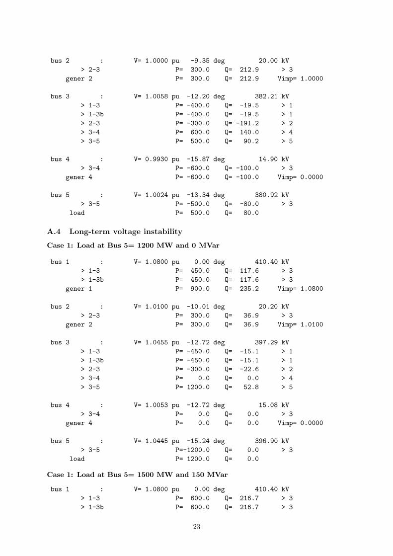
A.4 Long-term voltage instability

Case 1: Load at Bus 5= 1200 MW and 0 MVar

bus 1 : V= 1.0800 pu 0.00 deg 410.40 kV

> 1-3 P= 450.0 Q= 117.6 > 3

> 1-3b P= 450.0 Q= 117.6 > 3

gener 1 P= 900.0 Q= 235.2 Vimp= 1.0800

bus 2 : V= 1.0100 pu -10.01 deg 20.20 kV

> 2-3 P= 300.0 Q= 36.9 > 3

gener 2 P= 300.0 Q= 36.9 Vimp= 1.0100

bus 3 : V= 1.0455 pu -12.72 deg 397.29 kV

> 1-3 P= -450.0 Q= -15.1 > 1

> 1-3b P= -450.0 Q= -15.1 > 1

> 2-3 P= -300.0 Q= -22.6 > 2

> 3-4 P= 0.0 Q= 0.0 > 4

> 3-5 P= 1200.0 Q= 52.8 > 5

bus 4 : V= 1.0053 pu -12.72 deg 15.08 kV

> 3-4 P= 0.0 Q= 0.0 > 3

gener 4 P= 0.0 Q= 0.0 Vimp= 0.0000

bus 5 : V= 1.0445 pu -15.24 deg 396.90 kV

> 3-5 P=-1200.0 Q= 0.0 > 3

load P= 1200.0 Q= 0.0

Case 1: Load at Bus 5= 1500 MW and 150 MVar

bus 1 : V= 1.0800 pu 0.00 deg 410.40 kV

> 1-3 P= 600.0 Q= 216.7 > 3

> 1-3b P= 600.0 Q= 216.7 > 3

23

gener 1 P= 1200.0 Q= 433.5 Vimp= 1.0800

bus 2 : V= 1.0100 pu -14.79 deg 20.20 kV

> 2-3 P= 300.0 Q= 212.6 > 3

gener 2 P= 300.0 Q= 212.6 Vimp= 1.0100

bus 3 : V= 1.0166 pu -17.58 deg 386.30 kV

> 1-3 P= -600.0 Q= -23.9 > 1

> 1-3b P= -600.0 Q= -23.9 > 1

> 2-3 P= -300.0 Q= -191.4 > 2

> 3-4 P= 0.0 Q= 0.0 > 4

> 3-5 P= 1500.0 Q= 239.3 > 5

bus 4 : V= 0.9966 pu -17.58 deg 14.95 kV

> 3-4 P= 0.0 Q= 0.0 > 3

gener 4 P= 0.0 Q= 0.0 Vimp= 0.0000

bus 5 : V= 1.0089 pu -20.93 deg 383.37 kV

> 3-5 P=-1500.0 Q= -150.0 > 3

load P= 1500.0 Q= 150.0

Case 2: Higher Power generation

bus 1 : V= 1.0800 pu 0.00 deg 410.40 kV

> 1-3 P= 525.0 Q= 186.5 > 3

> 1-3b P= 525.0 Q= 186.5 > 3

gener 1 P= 1050.0 Q= 373.0 Vimp= 1.0800

bus 2 : V= 1.0100 pu -11.10 deg 20.20 kV

> 2-3 P= 450.0 Q= 197.6 > 3

gener 2 P= 450.0 Q= 197.6 Vimp= 1.0100

bus 3 : V= 1.0205 pu -15.26 deg 387.81 kV

> 1-3 P= -525.0 Q= -39.5 > 1

> 1-3b P= -525.0 Q= -39.5 > 1

> 2-3 P= -450.0 Q= -159.7 > 2

> 3-4 P= 0.0 Q= 0.0 > 4

> 3-5 P= 1500.0 Q= 238.6 > 5

bus 4 : V= 1.0005 pu -15.26 deg 15.01 kV

> 3-4 P= 0.0 Q= 0.0 > 3

gener 4 P= 0.0 Q= 0.0 Vimp= 0.0000

bus 5 : V= 1.0129 pu -18.59 deg 384.90 kV

> 3-5 P=-1500.0 Q= -150.0 > 3

load P= 1500.0 Q= 150.0

Case 3: Higher Motor load

bus 1 : V= 1.0800 pu 0.00 deg 410.40 kV

> 1-3 P= 600.0 Q= 226.7 > 3

> 1-3b P= 600.0 Q= 226.7 > 3

gener 1 P= 1200.0 Q= 453.3 Vimp= 1.0800

24

bus 2 : V= 1.0000 pu -14.84 deg 20.00 kV

> 2-3 P= 300.0 Q= 177.3 > 3

gener 2 P= 300.0 Q= 177.3 Vimp= 1.0000

bus 3 : V= 1.0117 pu -17.67 deg 384.45 kV

> 1-3 P= -600.0 Q= -31.8 > 1

> 1-3b P= -600.0 Q= -31.8 > 1

> 2-3 P= -300.0 Q= -157.9 > 2

> 3-4 P= 600.0 Q= 139.5 > 4

> 3-5 P= 900.0 Q= 81.9 > 5

bus 4 : V= 0.9990 pu -21.30 deg 14.99 kV

> 3-4 P= -600.0 Q= -100.0 > 3

gener 4 P= -600.0 Q= -100.0 Vimp= 0.0000

bus 5 : V= 1.0091 pu -19.69 deg 383.46 kV

> 3-5 P= -900.0 Q= -50.0 > 3

load P= 900.0 Q= 50.0

25

“All-in-one” test system modelling andsimulation for multiple instability scenariosInternal Report

Report # Smarts-Lab-2011-002

April 2011

Principal Investigators:

Ph.D. Rujiroj LeelarujiDr. Luigi Vanfretti

Affiliation:

KTH Royal Institute of TechnologyElectric Power Systems Department

KTH • Electric Power Systems Division • School of Electrical Engineering • Teknikringen 33 • SE 100 44 Stockholm • Sweden

Dr. Luigi Vanfretti • Tel.: +46-8 790 6625 • [email protected] • www.vanfretti.com

“all-in-one”test system modellingand...

Documents