7'6; 2 2 - Altimetry Data and the

Elastic Stress Tensor of Subduction Zones

Final Report on the Research

Supported by Grant #NAG5-94

RF 4340

National Aeronaut.ics and Space Administ.ration

Goddard Space Flight Center

Greenbelt. Maryland 20771

(NaSA-CB- 181 182) ALTIfl!ZTEX E A Z A A 1 D THB 187-27340 E L U T Z C STPBSS 3EYSOR OF SDBEUCTIGIY Z O l E S E i n a l Beport, 1 Sep, 1980 - 28 Pet. 1987 (Texas A&LI Univ.) 46 F A v a i l : NTIS Unclas

A O ~ / M E a o i CSCL 086 63/46 0087612

Michele Caput,o

September 1, 1980 - February 28. 1987

. .

https://ntrs.nasa.gov/search.jsp?R=19870017907 2018-06-18T00:06:08+00:00Z

J a

?

1

ABSTRACT

The maximum shear stress (mss) field due to mass anomalies is estimated in

the Apennines, the Kermadec-Tonga Trench, and the Rio Grande Rift areas and

the results for each area are compared to observed seismicity.

A maximum mss of 420 bar was calculated in the Kermadec-Tonga Trench

region a t a depth of 28 km. Two additional zones with more than 300 bar mss were

also observed in the Kermadec-Tonga Trench study. Comparison of the calculated

mss field with the observed seismicity in the Kermadec-Tonga showed two zones of

well correlated activity.

The Rio Grande Rift results showed a maximum mss of 700 bar occurring east

of the rift and at a depth of 6 km. Recorded seismicity in the region was primarily

constrained to a depth of approximately 5 kin, correlating well to the results of the

stress calculations.

Two areas of high mss are found in the Apennine region: 120 bar at a depth of

55 k m , and 149 bar at the surface. Seismic events nlwerved in the Apennine area

compare favorably to the mss field calculated. exhibiting two zones of activity.

The case of loading by seamounts and icecaps are also simulated. Results for

this study show that the mss reaches a maximum of about 1 / 3 that of the applied

surface stress for both cases, and is located at a depth related to the diameter of

the surface mass anomaly.

2

INTRODUCTION

The determination of the stress tensor in the earth’s crust is one of most

fundamental problems in geophysics. In quantitative seismology, an accurate

estimate of this tensor is of great value in both earthquake prediction and hazard

reduction; it would also allow to attempt a tentative estimate of the energy release,

source type and consequently the ground acceleration of future earthquake events

(e.g. Aki, 1968; Caputo, 1981; Hanks,1979).

The determination of the elastic stress tensor in the lithosphere is also of

importance in studying the dynamics of subduction and rift zones. Estimates of

the limiting values of the elastic parameters of the material involved as well as the

trajectories of the principal stresses could be made in these areas from the stress

field and then compared to the observed fault plane solutions in order to discuss the

previous motions of the crust and/or the relevance of this stress field with respect

to that generated by other forces.

Regions which exhibit active seismicity include oceanic and cont inental rift

zones, as well as active subduction zones. In most regions of active seismicity, the

regional stress field is complex and is induced by several interacting components.

In subducting plates, the applied vertical load. due to overburden pressure, creates

an important vertical component in the stress field. Important lateral components

are also created by existing horizontal forces, such as slab push or slab pull, both

related to lithospheric plate motion. -41 continental rifts, various combinations of

compressional and extensional forces. and overburden pressure interact to form the

total stress field. In order to effectively study the various aspects and implications

of the stress field, the individual components should be isolated.

3

The magnitude, value, and direction of maximum shear stress in the subsurface

may be computed mathematically if the regional stress field tensor is known, which

in turn requires the knowledge of the forces causing the field. The phenomena

which produce stress within the earth include: thermal processes and forces which

ultimately drive the plates, lateral variations of pressure on the ocean floor,

tidal forces, topographic loads, and in general, body forces associated to density

anomalies. In studying the regional stress field, one would have to consider all of

the above forces as sources of stress.

Numerous authors have dealt with stresses arising from tectonic forces, but,

inspite of its importance (Jeffreys, 1976), until recently little research on the stress

generating capacity of topography, its associated isostatic compensation, or gravity

anomalies has been carried out (Caput0 et al., 1985; Barrows and Langer, 1981).

Knowledge of this component of the stress field is important when attempting to

determine the stress due to a particular mechanism; i.e., the topographic-isostatic

generated component of the total stress field must be calculated and removed. The

c t r o r r G,lA .-,l,;”L L - - L,,, -+..A:,A ;., -,.-4 A, .+- : l :- 4 L - L J.., 4 - - 1 - 4 - :-4 ^ _ ^ ^ 4:-- “ ILL0.J **-*LA .,1*1L11 1 L u . 3 VC-L*, O U U U I L U 111 I I I V O L ULIu.11 1 3 C l 1 u . b uuc b W ylalL l l l l c l a L b 1 w l I .

primarily tectonic forces at plate boundaries (e.g. Nakamura and Gyeda, 1980).

The aim of this research is to determine the stress field in three regions with

different geodynamic conditions: the Kermadec-Tonga region, the Rio Grande Rift

and the Apennines. The results for each region will be compared to the observed

seismicity to see if stresses arising from mass anomalies play a role in earthquake

generation. In addition, the stress field associated with crustal loading caused by

seamounts and icecaps will also be examined.

I i

4

METHOD

To estimate the stress field we will assume the earth to be layered, have

spherical symmetry and use the formulae of Caputo (1961, 1984) which allow

to compute the deformation and stress field caused by body forces and surface

tractions.

For the discussion of the regions considered, it is sufficient to assume an earth

model consisting of two layers and a core, each homogeneous and isotropic. In

addition, we also assume an axisymetric distribution of body forces and surface

tractions which allows to approximate the two dimensional distributions of body

forces and surface tractions of the the three regions considered. The prescribed

surface stress is defined on a ring or a polar cap, independent of 4, the longitudinal

coordinate, acting radially inward. This surface stress is defined in the upper

hemisphere, 0<8<: (where 8 is the colatitude), in the form of a sum of Legendre

Polynomials up to the order 1000. Equal forces and tractions are applied in the

luwer hemisphere, FOli?, in order to insure that the sphere will not accelerate.

The two opposite loads are prescribed at the colatitudes of about in order

to minimize their interactions.

and

The density function for the body force is defined in the same manner as the

surface stress. It is a sum of spherical harmonics and is independent of the longitude.

The density acts throughout the volume of the layer and takes into account lateral

density contrasts within the layer. It is instructive to think of the density anomaly,

and consequently the associated body force. as acting in a manner consistent with

the Pratt hypothesis of isostasy. If the density function at any point is negative,

it implies a buoyancy force, while a positive density function implies a lithostatic

pressure.

5

KERMADEC-TONGA TRENCH

For the Kermadec-Tonga region, the lithospheric model is obtained to match

both the SEASAT, GEOS-3 altimetry data and Synbap bathymetry data. Both

the SEASAT and GEOS-3 altimetry data is used to obtain a measurement of the

geoid across the trench and calculate a geoid anomaly. The anomaly data base has

a value every 7 kilometers, with a vertical accuracy to within 10 centimeters. The

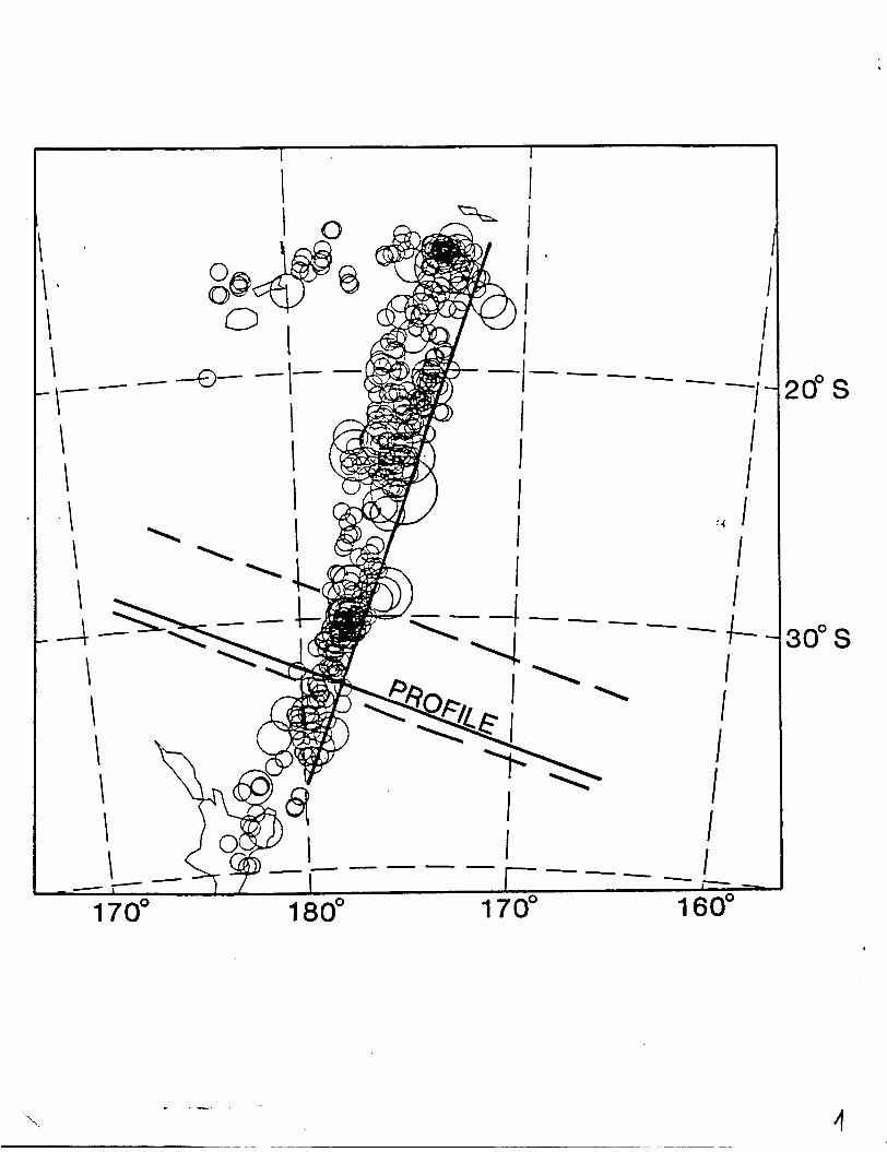
satellite track used is located at approximately 33" south and runs from northwest

to southeast, perpendicular to the trench. The satellite track used is shown in

figure 1 and is actually a compilation of many satellite tracks, taking all data which

intersected the track line. This is done in order to obtain a profile perpendicular to

the trench axis. The Synbap data is used to control the bathymetry of the study

region.

The lithospheric model (see fig. 1)consists of approximately 99 vertical

polygons over a horizontal extent of 2800 km. or one column centered every 28 km,

with a depth of 7.5 k m . These columns are further divided and assigned densities

which corresponded to the crust.al structure. The model is generated by assuming

that the density of the crust is 2.85 g - ~ m - ~ (Carlson and Raskin, 1984) and that

the lower lithoshpere has a density of 3.65 g - ~ m - ~ . In addition, the density model

also takes into account the density increase with time of the oceanic lithosphere

(McAdoo and Martin. 1984). The resulting density model, figure 1. has an oceanic

crust 8 km thick seaward of the trench and 15 to 20 km thick landward.

In this lithospheric model. the oceanic lithosphere has been assumed to vary

in density with time at a rate of 0.2.10-3 g . c n r 3 Myears. This low rate density

variation together with the variations in the thickness of the oceanic crust, the

thinner oceanic lithosphere landward of the trench, and the thinner downgoing slab

6

are responsible for the long wave length geoidal undulation observed by GEOS-3

and SEASAT.

The thickness obtained for the crust seaward of the trench comes close to

matching the defined thickness of 6 kni interpreted from a discontinuity surface in

the velocities of the seismic waves found at a depth of 6 km below the ocean bottom

(Shor et al., 1970; Turcotte and Shubert, 1982).

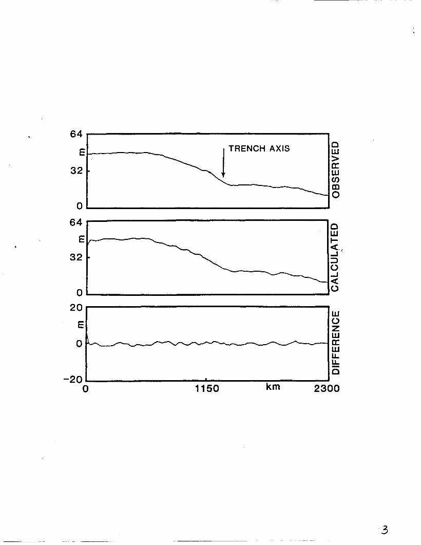
Figure 3 shows the actual geoid, the calculated geoid and the difference between

the two across the trench. The inversion matches the geoid with a difference of no

more then 3 meters, 1 meter in most instances (i.e. less than 10% of the maximum

undulation).

Results

With the topographic and density models it was possible to calculate the

stress field which they cause and ultimately the maximum shear stress field of the

Kermadec-Tonga Trench region. Layer one cont a im a lithostatic load, accounting

for the load of the bathymetry, and has a thickness of 8 km. Layer two is used to

simulate a buoyant force and was given a thickness of 20 kni.

The resulting mss field computed from the input is displayed in figure 4. In

the figures displaying the calculated ~ n s s field. certain symbols are used to portray

the orientation of the mss planes. A cross represents the trace of the mss planes

when the maximum and minimum principal stress axes are in the plane of the

page. A solid line depicts the maximum stress axis when the minimum stress axis

is perpendicular t,o the plane of the page. ,4n arrow represents the minimum stress

axis when the inaxiinuiii stress axis is perpendicular to the plane of the page. The

plane of the figure is the 6, 8 plane (t,he meridian plane).

For the figures re!at#ing to observed seismicity, the size of the circle represents

r

1

the realtive strength of the recorded event. A cross represents an event for which

a determination of body-wave magnitude was not made, but for which a depth

estimate was made. The bathymetric highs at 43.5" and 45.5" produce highs of

346 bar and 430 bar respectively at the layer one-layer two interface. In addition,

there are relative maxima of 295 bar and 221 bar at the lower interface of layer two,

at the same colatitudes as the highs observed at the upper interface. The stresses

calculated in the Kermadec-Tonga st,udy are meaningful for depths of 8 km or more,

due to the modeling procedure. In the core of the model, a relative high of 113 bar

is recorded at 45.5'. An area of low mss, less than 100 bar, is also shown in the

vicinity of the trench at, 47".

In conclusion, there are three areas of significant stress in the Kermadec-Tonga

Trench, a t the layer one-layer two interface, at the layer two-core interface and

within the upper part of the core at a dept,h of about 65 km.

Seismici t. y

The criterion used in selecting earthquake events is based on the need to

compare hypocentral locations with t h e areas of high mss caused by the topography

and density anomalies, which are determined in this paper. Therefore, only

earthquakes recorded after 1964, with an average body-wave magnitude, nib, greater

than 5 .5 , well constrained epicentral coordinates and depths above 250 km are used

in the correlation. Events restrained to normal depth, 33 km, are also included to

give some indication as to shallow seismicity. A total of 438 events meets the above

criteria. and provides a data base from which to work: in figure 5 the diameter of

the circle indicates the relative magnitude of the recorded event. The data for this

study comes froin the catalogues of the National Earthquake Information Service.

Figure 1 shows tlie regional seismicity in the Leriiiadec-Tonga area. The largest

8

event recorded in this area was of magnitude 7.0 and is closely associated with the

subduction of an apparently aseismic ridge at approximately 25" south. Above 25"

south, the seismicity is not constrained so closely to the trench axis as is the case

in the southern half of the system.

The distribution of earthquake events in the entire study region indicates that

over 50% of events above 100 km depth occur between 32 and 37 kin. This large

number is due in part to the fact that events considered to be shallow, but with

less than enough reported data to achieve an accurate depth estimate, are assigned

a depth of 33 km. Between 14 and 19 km depth, 17 events were recorded, between

38 and 43 km depth 20 events, and between 49 and 54 kin depth 22 earthquakes.

The earthquake data also indicate that over 70 % of events occur within 1.2" east

of the trench system.

To study more closely the seismicity in the region, the area was divided into

6 zones along and perpendicular to the trench. It is of interest to note that the

northern end of the trench system exhibits more shallow activity than does the

. 1 ' 1 1 A 1 1 1 . 1 1 scuthciii c ~ d , aiid that o v c i d l thc s<isiiij<itr< assvii&icci w l t 1 1 t l l r >uuuuc t l l i g ~ L ~ L U

has a very steep distribution.

Of particular interest in this study is the seismicity shown in figure 5 and

pertinent to the zone limited by t h e dashed lines of figure 1. This zone contains

our satellite track data. It is seen that nearly all of the seismicity is within 3" of

the trench axis, mostly on the west side. For this study, events above 100 km were

used. Between 32 and 35 kin depth there were 37 events recorded. including those

assigned the default value of 33 kin. Between 42 and 47 kni, 11 events were seen,

and between 10 and 15 km 5 events. The majority of activity occurs within 1" of

the trench axis in zone 2.

Comparing the seismicity to our calculated mss field we see that the highest

mss is located within 2" of the trench axis, which is where the highest, density of

observed seismicity is located. The depth da ta indicates shallow activity around

the trench. Our calculated stress field shows this feature nicely in the fact that high

mss are present above 70 km only, the deeper activity being due primarily to slab

mechanics. The seismicity around 30 km depth corresponds well to the depth of

our lower layer two interface.

10

RIO G R A N D E RIFT

In order to compare the stress tensor field in different geodynamic conditions,

we considered the Rio Grande Rift province as an example of continental rift. As

in the Tonga-Iiermadec Trench region, we considered the stress field generated by

the load of the topography and by the density anomalies at depth. The density

anomalies (see fig. 7) at the 39 degree north profile across the rift

province have been obtained using Bouguer anomalies as well as other constraints

derived from heat flow, seismic refraction profiles and magnetic surveys.

6 and fig.

For the Rio Grande Rift study we developed an inverse model (see fig. 8)

which fit the observed Bouguer gravity anomaly of Eaton (1986). The gravity

survey crosses the Rio Grande Rift zone at approximately 39" north. While the

overall Bouguer anomaly is negative, it is seen that over the axis of the rift there is

a very distinct gravity low of -333 mgals.

We considered that the lithosphere below the rift is thinned due to regional

extensional stresses, allowing the rise of a buoyant ast henospheric plume, which

creates the topographic ridge and extensional tectonics associated with the rift and

Southern Rocky Mountains. The lithospheric model assumes that the densities vary

laterally due to the geothermal gradient and isotherms associated with the rising

asthenospheric plume: in general, density values increase moving away from the rift

axis to the east and west.

In developing the density model. seismic studies of the Alvarado uplift were

used to control the crustal structure. The MohoroviEit discontinuity was defined

by using the results of the research conducted by Allenby and Schnetzler (1983), in

which all existing refraction lines 011 the North American continent were surveyed

to contour the depth of the Moho. Studies of P wave velocities by Baldridge et

11

al. (1984) were used to delineate the structure of the asthenosphere. Figure 6 shows

the final density model developed for the Rio Grande Rift study.

The area of study is divided into 90 vertical columns, each centered every 20 km

and with a thickness of 160 km. These vertical columns are subdivided horizontally

to model the actual structure containing five distinct units: asthenosphere, mantle,

lower crust, upper crust, and sediment layer. The subcolumns were then assigned

densities which matched the the observed gravity anomaly and seismic velocity data.

The densities of the model west of the rift axis are required to remain low in order

to mirror the lateral geothermal gradient and to account for the Bouguer anomaly

across the Colorado Plateau and the Basin and Range Pro\. mce.

In the model developed, the computed gravity anomaly deviates from the

observed by less than 1 percent. of the entire long wavelength anomaly low of -

333 nigal over the rift province. Figure 7 shows both the observed and calculated

gravity profiles for the study area.

Results

From the density model, it was possible to develop appropriate input for the

Earth model to calculate the mss field. Layer one. as in the Kermadec-Tonga

st>udy, contains a lithostatic load to account for topography. Layer one was given a

thickness of 6 km. Layer two was again used to simulate buoyant forces generated

by density contrasts a t deeper depths, and was assigned a thickness of 45 km.

The mss in the region caused by the density anomalies inferred from the gravity

anomalies and seismic velocity data in the Rio Grande Rift region are illustrated

in figure 9. We may see that the highest niss occur near the layer one-layer two

interface, a depth of about 6 km, and reaches a magnitude of approximately 700 bar.

The overall character of the calculated niss field is compressional, which is evident

12

from the orient*at.ions of mss planes and the associated principal axes. These planes

exhibit high angle thrust mechanisms for the release of stress.

The overall magnitude and orientation of the mss field is primarily a function

of the large lithostatic load present in layer one and the equally large buoyant force

in layer two. Although t,he magnitudes calculated may be in excess of those in the

Rio Grande area, due to the large overburden pressures, acceptable changes in the

thicknesses and densities of the two layers would not alter bhe t.he distribution and

character of the stress field calculated.

Seismici t ~7

Figure 6 shows the observed seismicity in the Alvarado Ridge area. Crosses

represent events for which depth estimates are made, but body-wave magnitude

values are not well defined, with the diameter of the circle indicating the relative

magnitude of the recorded event; crosses represent events with depth estimates but

body-wave magnitudes are not well defined. A total of 124 events were found in the

area which f i t the criteria: events occurring after 1964 with calculated hypocentral

depths. Over 70 rC of the events occur around 6 kni depth, while 11 % occur near

33 km depth. Of the 124 events assigned a magnitude value, 29 were between 4.5

and 4.7 mb.

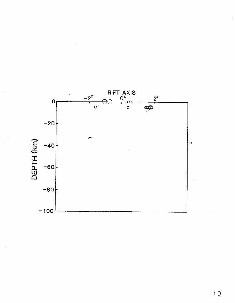
Again, the area is divided into zones for further study. Of primary interest to

this study is the section, shown in figure 10. which contains our density model and

calculated niss field. This section contains 29 events with epicenters between the

dashed lines of figure 6. 21 events. or nearly 72 % of the seismicity recorded in zone

5 , occurred near 5 k m depth, wi th 2 events occurring at 33 km depth. The lateral

distribution of observed earthquakes. indicates that over 65 Y, of events occurred

to ?he east of the rift a i s at distances greater than 1.45".

13

By comparison with the calculated mss field in the Rio Grande Rift area, we

see that the events which occur at 6 km depth are in agreement with the depth

at which the highest mss values occur. Also, the lateral distribution of seismicity

compares nicely to the zone of highest niss calculated, to the east of the rift.

In summary, the earthquake data shows that the Alvarado Ridge, and in

particular the Rio Grande Rift, seismicity is characterized as shallow in depth

with magnitudes values much less than in the Kermadec-Tonga Trench area, but

is associated to a mss field which reaches values at least twice as large as those of

the Kermadec-Tonga Trench in the areas of high seismicity.

The normal faulting mechanism of the earthquakes of this extension area

(Eaton, 1986) is in agreement with that which would be generated by the mss

field computed, shown in figure 9.

14

APENNINES

To study the stress tensor in one more geodynamic condition, we considered

also the Apennines where apparently we have the condition of a terminal collision of

two continental margins (Boccaletti et al.: 1980) with the negative gravity anomalies

displaced about 50 km with respect to the axis of the mountain range.

The data used for this study is derived from a Bouguer gravity map of Italy,

produced by the Italian National Council of Research and entitled the Modello

Strutturale D'Italia. At approximately 43" north, two very distinct features are

observed (Mongelli et al., 1980, Caputo et al., 1984, 1985): a gravity high of +30

mgals in the central Apennines, and a very distinct gravity low of approximately

-60 mgals displaced approximately 50 km to the east of the Apennine range. This

is the area of interest and the profile considered is shown in figure 11.

The crustal thicknesses used were based on the work of Caputo et al. (1976),

in which seismic horizons in eastern Italy were delineated by using surface wave

dispersion. In his investigation, t w o distinct aeisniic zones were mapped. The

conclusion drawn was that the upper crust extends to a depth of 30 km, with a

second layer between 30 and 55 km.

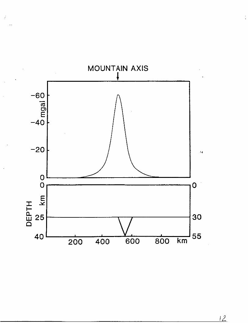
The inversion of the gravity data demonstrated that for an anomaly in the

second layer, between 25 and 40 kni depth. producing a surface anomaly of -60

mgals, the maximum density anomaly would be approximately Ap = -0.175.

A more recent investigation of the crustal structure in Italy was conducted by

Morelli et al. (1986) using deep seismic soundings. This study indicates that the

first layer has a thickness of 25 km while the second a thickness of 15 km. Placing

the density anomaly in the second layer requires a contrast of -0.246 g - ~ m - ~ .

Both the topography and derisity anomalies ale modeled with a width of I",

15

corresponding to the average width of the Apennines, 100 km. Based on the average

height of the Apennines, with an average density of 2.67 g ~ m - ~ , the maximum

load of the mountain range is approximately 350 bar. The topography is centered

at 45", with the density anomaly centered at 45.5". The density models developed

are shown in figure 12. The premise followed was that the gravity low observed

indicated that the compensating root of the Apennines was displaced relative t o

the mountain range by half the width of the topography, or fifty kilometers.

Results

The mss field associated with the first crustal model is shown in figure 13. Note

the slightly curved nature of the contours. The maximum mss of 149 bar is located

at the surface, at 45.5" colatitude for case one. Also. a relative high mss of 120

bar is present at the lower interface of layer two. The vertical zone of 90 bar stress

is primarily centered about 45" in both layers one and two: we may also note the

slight perturbations of the contours in layer two. These results are in agreement

with those of Caputo et al. (1985) and confirm that when the isostatic compensating

mass is displaced with respect to the topographic load the inss is larger than when

they are exactly opposite.

It is seen that most mss planes are perpendicular to the meridian plane.

The upper right hand corner of the figure shows an area in which the minimum

principal stress axes are in the meridian plane and the maximum perpendicular.

The orientations of the niss planes a! thc mss highs were seen to be high angle?

indicating a thrust type mechanism for relieving stress.

Results for the second crustal model are shown in figure 14. Many of the same

features are seen in this figure as were in the previous. The major difference is the

depths a t which the maxima occur. The maxima still occur at the layer boundaries,

16

with a value of 90 bar a t the lower interface of layer two and 150 bar at the surface.

To simulate the effect of the stress field of the Apennines on the long time limit,

the rigidity of the core of the first model was successively lowered, while the other

parameters remained the same. The migration of the 300 bar field is examined.

The rigidities assigned to the core were: 5 x l o l o , 5 x lo9 , 5 x lo8, 5 x lo' and 0.

This approach is used to simulate a lower lithoshpere which deforms more readily

on geologic time scales, and to provide some idea of the long term stress build up

in the region, which in turn would set limits for the rigidity of the asthenosphere

for perturbations of very low frequencies. In addition, it may give some insight into

how the stress field changes thru time in this regime.

Figure 15 shows the effect of low rigidity in the core of the model in the

Apennine study. Note that the 300 bar field becomes very broad as the the model

core rigidity approaches zero, and their contorted nature above 45" colatitude. -41~0

note how the contours above 45" colatitude have migrated laterally, while little

movement of the contours below 45" has taken place. Assuiiiiiig that failure may

occur at 500 bar (Clark, 19661, we may infer that the rigidity of the asthenosphere

at the very low frequencies of interest in most geologic phenomena is more than

5 x l o* .

Seismicity

The regional seismicity for Italy is shown in figure 11. Again, the crosses

represent events for which depth estimates are made. but body-wave magnitude

values are not well defined. A total of 290 events were used. It is seen that

the earthquake magnitudes are significantly lower in the Italian area than in the

Kermadec-Tonga, with only 2 events between 5.9 and 6.0, while 256 events were

not assigned nib values. The greatest concentration of events for the region occurs

between 8 and 11.8 kni, with a relative high between 33 and 34 kin.

As in the other two study regions, the area was divided up into subareas or

zones. We will concern ourselves with events in zone 3, figure 16, which contains

the gravity anomaly we are interested in. It is seen that the seismicity in zone

3 is primarily constrained to above 50 km and located in two regions. The first

region is related to the Apennine mountain range and the second is located in the

Dinaric Alps of Yugoslavia. Examining the distribution of earthquakes, we see that

over 50% of them occur between 1 0 and 13.2 km depth, with a second grouping

containing 12 events between 33 and 34 km depth.

Comparing this to the results of our calculations. we see that the shallow events

related to the Apennine mountains correlate well with the high mss gradient present

directly above the density anomaly. Also, the events which fall between 33 and 34

km depth seem to be due the topography-density anomaly couple, although the

relevant mss field for these earthquakes seems a few kilometers lower.

We should also note tha t the mechanism of many of the deeper earthquakes of

the area (Gasparini et al.. 1978, 1979, 1980) is in agreement with that which would

be generated by the mss field computed and shown in figures 13 and 14.

18

CONCLUSIONS

The results of the study correlating the three mss fields calculated for the three

geodynamic areas with their observed seismicity indicates, at least to first order,

that the stresses generated from topography and density anomalies may play a

significant role in active earthquake regimes.

It is seen that in the Kermadec-Tonga Trench study that the bathymetric highs

produces mss highs of 346 bar and 430 bar respectively at the layer one-layer two

interface. In addition, there are relative maxima of 295 bar and 221 bar at the lower

interface of layer two, a t the same colatitudes as the highs observed at the upper

interface. In the core of the model, a relative high of 113 bar is recorded. An area

of low mss, less than 100 bar, is also calculated in the vicinity of the trench.

Comparing our calculated mss field to the observed seismicity in the Kermadec-

Tonga Trench, we see that the highest mss gradient is located within 2" of the

trench axis, which is where the highest density of earthquake events is located.

The distribution of event depths indicated shallow activity around the trench.

Our calculated stress field shows this feature nicely in the fact that high mss are

present above 70 km only; the deeper activity is therefore not due to the stress field

estimated here, but probably only to the subducting slab. The seismicity around 30

km corresponded well to the depth of our lower layer two interface. at which high

mss values are recorded.

Results for the Rio Grande Rift study show that the highest mss occurrs near

the layer one-layer two interface. at a depth of about 6 kin. and reachs a magnitude

of approximately 700 bar. The extent of the 700 bar field is to the east of the

rift. The overall niagnitude and orientation of the niss field calculated in the KO

Grande study is primarily a function of the large lithostatic load present in layer one

19

and the equally large buoyant force in layer two. Although the magnitudes of the

I I ~ S S calculated may be in excess of those in the Rio Grande area, due to the large

overburden pressures, the distribution and character of the stress field is preserved.

The observed seismicityin the Rio Grande area shows that the greatest number

of events occurred near 5 km depth, with 2 events occurring at 33 kin. The lateral

distribution of observed seismicity showed that over 65% of events'occurred to the

east of the rift axis at distances greater than 1.45'. These distributions compare

favorably to the calculated mss field, where the highest rnss values are recorded at

a depth of 6 km, with the largest zone of high mss to the east of the rift axis.

Finally, the study of the stress field in the Apennine area indicates that two

zones of high mss exist. For both crustal-density models considered, a maximum

rnss of about 150 bar is located at the surface, with a relative high mss of 120 bar

at the lower interface of layer two. A vertical zone of 90 bar stress is present in

both layers one and two. It is seen that most iiiss plants are perpendicular to the

meridian plane. The orientations of the niss planes at the mss highs are seen to be

high angle. indicating a thrust type mechanism for relieving stress.

The earthquake data for the Apennine area showed that the magnitudes are

significantly lower in the Italian area than in the Kermadec-Tonga. The seismicity

is primarily constrained to above 50 k m depth. The distribution of earthquakes

indicates that over 50% of the events occur between 10 and 13.2 kin depth, with

12 events recorded between 33 a n d 34 km depth. Comparing this to our stress

calculations for the Apennines. i t is seen that the shallow events. related to the

Apennine mountains, correlates well with the high inss gradient present directly

above the defisity a1;oiiialy. The eveI;ts v;hich fall beiweeii 33 and 34 h i depth

compare to approximately to the depth of our layer two-core interface.

20

APPENDIX

The last part of this research investigates the stress field produced when the

system is subjected to loading by antipodal caps without isostatic compensation.

Two cases are considered for simulation: loading by an ice cap and loading by a

seamount, both of which seem to be viable stress generating entities. Evidence

to suggest this generating capacity is clearly observed from glacial deflections and

rebound, and peripheral bulges near Pacific seamounts and large volcanoes. Because

of the nature of the stress generating structures in this section, no compensation is

assumed.

To simulate loading by an ice cap, the pressure cap was given a diameter

of 6" and a height of 2 km, corresponding to continental ice caps present during

Pleistocene glaciation (Turcotte and Shubert, 1982). With a density of 1.0 g ~ m - ~ ,

the iiiaxiiiiuiii applied surface stress was calculated to be 200 bar.

In order to examine loading by seamounts, the pressure cap is assigned a

diameter of 2", a height of 4 kIn and density of 2.8 g cmP3, simulating Pacific

seamounts of the northern Hawaiian Island chain (Turcotte and Shubert, 1982).

Neglecting the hydrostatic contribution of the water column, a maximum applied

surface stress of 1.1 kbar is used.

For both models. layer one is assigned a thickness of 35 km. layer two a thickness

of 50 km. The rigidity of layer one and two are assigned a value of p = while

the core is given a value of p = 5 x 10". Lame's parameter. A, is assigned a value

of 1.273 x 10" for all layers and core. Because of the sharp discont,inuities present

in the functions describing the topography, 1000 terms are used in the summat,ion

of the Legendre Polynomials dexribing them.

21

Result. s

Figures 1 7 and 18 display the mss field due t,o loading by a pressure cap,

simulating an ice cap and a seamount respectively. The most, striking feature in

both diagrams is the high mss located at. the colatitudes of the termination of the

cap. Not,e also t,he behavior along the axis of the applied surface stress in the ice

cap model.

The maximum mss is 70 bar for the ice cap model and 350 bar for the seamount

model, or a little over 1 / 3 of the maximum applied surface load. The maximum mss

for the seamount model occurs a t a shallower depth, 35 km, than for the ice cap

model, 85 km. This difference in depth is related to the width of the pressure cap:

stresses generated by short,er wavelength surface loads decrease more rapidly with

depth than longer wavelength features. It is interesting to note that. in both cases,

away from the center of the surface load, the maximum principal stress direction is

along the principal 6' axis and changes to the principal r̂ ' direction with increasing

depth.

22

The research associated to the solution of the problems of this project led to

the publication of the following papers:

Topography and its isostatic compensation as a cause of seismicity.

Tectonophysics, 79, 73-83, Caputo M., Milana G., Rayhorn J.

Relaxation and free modes of a self-gravitating planet. Geophys. J . R. ast. SOC.,

77, 789-808, 1984a, M. Caputo.

Topography and its isostatic compensation as a cause of seismicity, a revision.

Tectonophysics, 111, 25-39, 1985, Caputo M., Manzetti V., Nicelli R.

Spectral Rheology, Proceeding Symposium Space Techniques for Geodynamics.

Hungarian Acad. of Sc., J . Somogi, C. Rigberg Ed., 1984, M. Caputo.

Determination of the creep, fatigue and activation energy from constant strain

rate experiment. Tectonophysics, 91, 157-164, 1983, M. Caputo.

Nonlinear and inverse rheology of rocks. Tectonophysics, 122, 53-71, 1986,

M. Caputo.

Generalized rheology and geophysical consequences. Tectonophysics, 116,

163-172. 1985, M. Caputo.

The polfluchtkraft revisited. Boll. Geof. Teor. Appl., 28, 199-214, 1986,

M. Caputo.

The normal gravity field in space and a simplified model. At t i . Acc. Naz. Lincei,

Roma, 1-10, 1986, M. Caputo.

Wave number independent rheology in a sphere. Atti. Acc. Naz. Lincei, Roma,

1-34, 1986, M. Caputo.

The stress field caused by the topography in the Tonga, Rio Grande and

Apennine regions. Proceed. Symp. on the Lithosphere, Rome, 1987,

Caputo M., Marten R., Mechani B.

23

The normal gravity field in space and the free air anomalies: rigor and

consequences. Proceed. Wegener Symposium, Bologna, 1987, M. Caputo,

R. Caputo.

and to the following dissertations and theses:

Wainright E.J., Calculation of isostatic gravity anomalies and geoid heights

using two dimensional filtering: implications for structure in subduction

zones, Ph.D. Dissertation, Graduate College of Texas A&M University,

1983.

Christian B.E., Utilization of satellite geoidal anomalies for computer analysis

of Geophysical models. Master Thesis, Graduate College of Texas A&M

University, 1985.

Sevuktekin M.T., The estimate of the shear stress field of a self gravitating

elastic planet during its formation. Master Thesis, Graduate College of

Texas A&M University, 1984.

Marten R., The propagation of the stress due to the ridge push. Master Thesis,

Graduate College of Texas A&M University, 1986.

Mecham B., The distribution of maximum shear stress in subduction zones due

to topography and isostatic compensation. Master Thesis, Graduate

College of Texas A&M University, 1986.

Benavidez A.. Pattern recognition of earthquake prone areas in the Andes,

P1i.D. Dissertation. Graduate College of Texas Ad-M University, 1986.

24

R.EFERENCES

Aki, K., 1968, Seismic Displacement Near a Fault: J. Geophys. Res., 73, 5359- 5376.

Balderidge, W. S., Olsen, K. H. and Callender, F. J., 1984, Rio Grande Rift: Problems and Perspectives, in Rio Grande Rift: Northern New Mexico, Eds. W. S. Balderidge, P. W. Dickerson, R. E. Riecker and J. Zidek: New Mexico Geological Society Guidebook, 35th Field Conference.

Barrows, L. and Langer, C. J., 1981, Gravitat,ional Potential as a Source of Earthquake Energy: Tectonophysics, 76, 237-255.

Boccaletti, M., Coli, M. and Decandia, A., 1980, Evoluzione dell’Appennino settentrionale second0 un nuovo modello strutturale: Mem. SOC. Geol. Ital., XXI, 359-373.

Caput.0, M., 1961, Deformation of a Layered Earth by an Axially Symmetric Surface Mass Distribution: J . Geophys. Res., 66, 1479-1483.

Caputo, M., 1981, Earthquake Induced Ground Acceleration: Nature, 291, 51- 53 .

Caputo, M., 1984, Relaxation and Free Modes of Self-Gravit,ating Planet: Geophys. J.R. Ast,r. SOC., 77, 789-808.

Caputo, M., Iinopoff, L., Mantovani, E., Muller, S. and Panza, G., 1976, Rayleigh Phase Velocities and Upper Mantle Structure in the Apennines: Ann. Geofis., 29, 199-214.

Caputo, M., Milana, G., and Rayhorn, J., 1984, Topography and its Isostatic Conipensation as a cause of Seismicity in the Apennines: Tect.onophysics, 102, 333-342.

Caputo. 11.. Manzetti, IJ-.. Nicelli, R.: 1985. Topography and its Isostatic Compensation as a cause of Seismicity; A Revision: Tectonophysics, 111, 25-39.

Carlson, R. L. and Raskin, G . S., 1984, Density of the Ocean Crusts: Nature. 311, 555-558.

25

Clark, S. (Ed.), 1966, Handbook of physical constants: Geol. SOC. Am. Memoir. 97

Eaton, G., 1986, Topography and Extensional Origin of the Southern Rocky Mountains and -4lvarado Ridge: Geologic Society of London, Special Publi- cat.ion. In Press

Gasparini, G., Iannaccone, G., and Scarpa, R., 1980, On the focal mechanism of italian earthquakes: Rock Mechanics, Suppl. 9, 85-91.

Gasperini, M., and Caputo, M.. 1978-1979, Preliminary study of the Upper Mantle in the Tyrrhenian Basin by Means of the Dispersion of the Rayleigh Waves: Rivista Ital. di Geofis. e Meteor., Vol. V, (in onore di M. Bossolasco). 146-149

Hanks, T. C., 1979, b Values and Seismic Source Model: Implications for Tec- tonic Stress Variations Along Active Crustal Fault Zones and the Est,imation of High Frequency Strong Ground Motion: J . Geophys. Res., 84, 2235-2242.

Jeffreys, S. H., 1976, The Earth: Cambridge University Press, Cambridge.

McAdoo. D. C. and Martin, C., 1984, SESAT Observations of Lithosphere Flext.ure Seaward of the Trenches: J . Geophys. Res., 89, 3201-3210.

Rilongelli. F.. Loddo, M., and Calcagxiile,, 1975: Some observations on t.he Apennines gravity field: Eart.11 and Plan. Sci. Lett., 24, 385-393.

Morelli. C., Personal communication: 1986.

Nakamura. E;. and llyeda, S., 1980, Stress Gradient in Arc-Back Regions and Plate Subduction: J . Geophys. Res., 8 5 , 6419-6428.

Shor, G . G.. hilenard, H. W., Raitt, R. IT., 1970, Structure of the Pacfic Basin, in The Sea, Eds. A . Maxwell: W-yley-Interscience.

Turcot,te, D. and Schubert, G.. 1982, Geodynamics: John VC’iley k Sons, New York.

Figure

LIST OF FIGURES

1. Observed seismicity in the Kermadec-Tonga Trench region. Also shown is the profile used in this study. The dashed lines limit the zone in which earthquake data is used for comparision.

The density model used to match the observed geoid across the Kermadec-Tonga Trench along the profile. Density values are shown. . . . . . . . . . . . . . . . . . . . 2

The observed geoid, calculated geoid and difference between the two across the Kermadec-Tonga Trench along the profile.

. . 1

2.

3. . . . 3

4. MSS field for the Kermadec-Tonga Trench study. Contour interval is 100 bar. See text for explanation of symbols used. . . . . 4

5. Observed seismicty, within the zone limited by the dashed lines of figure 1, as a function of depth and angular distance from t,he axis for the Kermadec-Tonga trench. . . . . . 5

6. Observed seismicity in the Rio Grande Rift region. Also shown is the profile used in this study. The dashed lines indicate the zone in which earthquake data was used for comparision. 6

7 . Comparision of model gravity anomaly (heavy line) with the observed Bouguer anomaly at, the 39" north profile (light line) for the Rio Grande Rift study. . . . . . . . . . . . . 7

8. The density model used to match t.he observed gravit.y anomaly across the Rio Grande Rift along the 39" profile. Numbers indicate base densities for each unit defined. . . . . . . . MSS field for the Rio Grande Rift study. Contour interval is 100 bar. See text for explanation of symbols used.

8

9 9.

. . . . . . . 10. Observed seismicty, within the dashed zone of figure 6 :

as a function of depth and angular distance from the rift axis for the Rio Grande study. . . . . . . . . . . . . . . . . . . 10

Observed seismicity in the Apennine region. Also shown is the profile used in this study. The dashed lines indicate the zone in which

11.

earthquake data was used for comparision with the mss field computed. 11

LIST O F FIGURES (Continued)

Figure

12.

13.

14.

15.

16.

17.

18.

Gravity inversion model used to obtain the -60 mgal gravity anomaly present in Apennine area. The dashed lines indicate the second crustal model used for the study. . . . . . . . . . . . . 12

MSS field for the first Apennine model. Contour interval is 30 bar. See text for explanation of the symbols used. . . . . . 13

MSS field for the second Apennine model. Contour interval is 30 bar. See text for explanation of the symbols used. . . . . . 14

Migration of the 300 bar contour as the rigidity of the core is lowered. Numbers indicate the rigidity of the core. . . . . 15

Observed seismicty, within the zone limited by the dashed lines of figure 15, as a function of depth and angular distance from the mountain axis for the Apennine stsudy. . . . . 16

MSS field due t,o loading by an ice cap, p1 = p ? , p3 = 0 . 5 ~ ~ . Cont,our interval is 10 bar. . . . . . . . . . . . . 17

MSS field due to loading by a seamount. pl = p2, p3 = 0 . 5 ~ ~ . Contour interval is 100 bar. . . . . . . . . . . . . 18

20" s

30" S

0

-300 n E Y - -600

-c I -

.O 168 -0 167 I 1

-0105

-01 10

-0125

I

2

64 1 1

J 20 E

0 1

-20 I A

01 I

w 0 z W [I w LL 11 0 -

64

E

32

n w

0

3

20" s

30" S

TRENCH AXIS -2O O0 2 O - 4 O

0

-20

I -40 I- n n W

-60 @-*

-80

-100

5

l l

I & R 1 %

I

- - -- 11o"w 105"W

45"N

40"N

35"N

30"N

6

-100

-200

-300

7

n

E s I I-

W

W

n n

0.

80-

107-

133.

160.

SEDIMENT

ASTHENOSPHERE

3.23

5 - .- >'A --

I I I I 1 0 360 720 1080 1440 1800

- 4 O

RIFT AXIS f - 2 O O0 2 O 4 O

9

n f Y

I I- Q W

w

n

0

-20

-40

-60

-80

-100

RIFT AXIS -2O I nn OO^. 2 O

I VI - I

0 9-

a .

1 3

i 0"E 12"E 14"E

44"N

42"N

40"N

16"E

-60

-40

-20

0 0

MOUNTAIN AXIS

\ f

\I I I V I I

200 400 600 800 km 40r

0

30

55

MOUNTAIN AXIS 1

0

10

20

30 30

n t 2 40 W

50 w

55 n

135 1:

IC

-6 X 4 + % X % + + 215:~ X Z 4 + % X x 4 4

X 4 + + x X X % 4

295 11 Y 4 + + % X X x 4

r 4 4 + + % X X % 4

375& 3 1 1 I -I r m ” n T - 4 3 O 4 4 O 4 5 O 4 6’ 4 7 O 4 8’

COLATITUDE

13

1 - lo 0"

MOUNTAIN AXIS

0

10

20

lo 2 O

b r\ f .. Y I Y 1 I

" ,. +.

. n

Y x X X + + + % X v

0 0 W

I X X X + + T X X X

407 n -! 1 v ,.

I I- Q w 40 Y " 7 Y 1 I ., n n Y Y -

Y 1 Y I - I .y

I I

SO+ x x 4- + 3- % % >:

% 4- % + % -A 1

7:

I

.t + % X .t- + j. % 7L

I

120 -r % 4- + % X % + + % '1:

3 , I I -I Y b I I c\ I 1 I d 3-

MOUNTAIN AXIS i 0

30

COLATITUDE

-2O 0

-20

n E Z -40

I: I-

W

e -60 -80

-100

MOUNTAIN AXIS -lo O0 lo 2 O

X

9 W'

x x x >

X

53 X

3 X

n

z E

r

a

w

I- l l W

0

10

20

30

40

50

60

70

80

7

U W t J a

cv U W t ,I a

W U 0 0

0:O 1:O 210 3:O 4.0 5.0 6.0 7.0 8.0

COLATITUDE (e)

17

40

1: + + % Y-

n

E Y 50 W

I ' % $0 +

165 + + + % J-

1: X % + + + + -t

245 x x % -+ + + + + 285 *R

60 a.

'1L

L

80