altruistic transmit beamforming for cross-layer
TRANSCRIPT
Aalto University
School of Electrical Engineering
Degree Programme of Communications Engineering
Christos Karaiskos
Altruistic Transmit Beamforming forCross-layer Interference Mitigation inHeterogeneous Networks
Master’s Thesis
Espoo, December 14, 2012
Supervisor: Professor Jyri Hamalainen
Instructor: Dr. Alexis Dowhuszko
Aalto University
School of Electrical Engineering
Degree Programme of Communications Engineering
ABSTRACT OF
MASTER’S THESIS
Author: Christos Karaiskos
Title:
Altruistic Transmit Beamforming for Cross-layer Interference Mitigation
in Heterogeneous Networks
Date: December 14, 2012 Pages: 10 + 86
Major: Radio Communications Code: S-72
Supervisor: Professor Jyri Hamalainen
Instructor: Dr. Alexis Dowhuszko
The emergence of heterogeneous networks, with low-power nodes operating under
the umbrella of high-power macro cells, simplifies planning procedures for opera-
tors, but introduces the problem of cross-layer interference between the overlap-
ping cells. An effective technique for combating interference is transmit beam-
forming (TBF), a transmitter-side technique which utilizes partial knowledge of
the channel and presence of multiple antennas at the transmitter to enhance the
signal reception quality at a receiver. When applied to the base station associ-
ated with the receiver, TBF boosts the desired signal. On the other hand, when
applied to the interfering base station, TBF reduces the effect of the interference
signal. The former technique is commonly referred to as egoistic TBF, while the
latter is known as altruistic TBF. In this thesis, we provide theoretical evaluation
of the performance gains that altruistic TBF is able to offer to a heavily interfered
user in a heterogeneous setting, when channel state information is conveyed from
the receiver to the transmitter through a limited feedback channel. We show that
the application of altruistic TBF to specifically defined clusters of interferers is
able to drastically improve performance for the victim user. Furthermore, we
prove the exact upper bound for the performance of the victim user, when only
phase feedback is used for altruistic TBF and the source of interference is a sin-
gle dominant interferer. Finally, we investigate and propose new techniques that
can be applied to multi-antenna heterogeneous network scenarios for interference
mitigation purposes.
Keywords: heterogeneous networks, femtocells, interference mitigation,
MIMO, closed-loop methods, transmit beamforming, cross-
layer interference
Language: English
ii
Acknowledgements
This work is part of the Wireless Innovation between Finland and U.S. (WiFiUS).
More specifically, it was prepared in the context of the research project “Dis-
tributed Resource Allocation and Interference Management for Dense Hetero-
geneous Wireless Networks”, a collaboration between Aalto University and the
University of California-Davis.
I wish to thank Professor Jyri Hamalainen for the opportunity to participate
in the mentioned research project as a Master’s thesis worker and for the invalu-
able pieces of advice throughout the study. I would like to express my deepest
gratitude to Dr. Alexis Dowhuszko for our countless constructive discussions, his
helpful guidance and the positive energy in our collaboration.
I would like to deeply thank my parents for all the love and support throughout
good and bad times, and all relatives and close friends for always being there,
despite the distance. Finally, I would like to dedicate the present thesis to my
uncle Kostas and grandmother Stamatia, who I know are watching over me from
up above.
Espoo, December 14, 2012
Christos Karaiskos
iii

iv
List of Abbreviations
3G 3rd Generation
BS Base Station
BU Base Unit
CAPEX CAPital EXpenditure
CDF Cumulative Distribution Function
CL Closed Loop
CLT Central Limit Theorem
CoMP Coordinated Multi-Point
CS/CB Cooperative Scheduling/Beamforming
CSG Closed Subscriber Group
CSIT Channel State Information at the Transmitter
CU Central Unit
DCS Dynamic Cell Selection
DoA Direction of Arrival
DTD Delay Transmit Diversity
EGT Equal Gain Transmission
FBS Femto Base Station
FDD Frequency Division Duplex
v
FFR Fractional Frequency Reuse
FUE Femto User Equipment
GPS Global Positioning System
HetNet Heterogeneous Network
i.i.d. Independent and Identically Distributed
JP Joint Processing
JT Joint Transmission
LTE Long Term Evolution
MBS Macro Base Station
MISO Multiple Input Single Output
MUE Macro User Equipment
OL Open Loop
OPEX OPerational EXpenditure
OTD Orthogonal Transmit Diversity
PBS Pico Base Station
PC Power Control
PDF Probability Density Function
PPC Partial Phase Combining
PSTD Phase Sweep Transmit Diversity
QoS Quality of Service
RF Radio Frequency
RN Relay Node
RRH Remote Radio Head
vi
RV Random Variable
RVQ Random Vector Quantization
SDT Selection Diversity Transmission
SIC Successive Interference Cancellation
SINR Signal-to-Interference plus Noise Ratio
SNR Signal-to-Noise Ratio
STS Space Time Spreading
STTD Space Time Transmit Diversity
TAS Transmit Antenna Selection
TBF Transmit Beamforming
TDD Time Division Duplex
TSC Transmitter Selection Combining
TSTD Time Switched Transmit Diversity
TTI Transmission Time Interval
UE User Equipment
VQ Vector Quantization
WCDMA Wideband Code Division Multiple Access
vii

viii
Contents
1 Introduction 1
1.1 Motivation . . . . . . . . . . . . . . . . . . . . . . . . . . . . . . . 3
1.2 Problem Context . . . . . . . . . . . . . . . . . . . . . . . . . . . 4
1.3 Contribution . . . . . . . . . . . . . . . . . . . . . . . . . . . . . . 5
1.4 Thesis Organization . . . . . . . . . . . . . . . . . . . . . . . . . . 6
2 The Concept of Transmit Beamforming 9
2.1 Classification of Transmit Diversity Methods . . . . . . . . . . . . 9
2.1.1 Channel State Information at the Transmitter Side . . . . 10
2.1.2 Open-Loop Methods . . . . . . . . . . . . . . . . . . . . . 10
2.1.3 Closed-Loop Methods . . . . . . . . . . . . . . . . . . . . . 11
2.2 Transmit Beamforming and MISO System Model . . . . . . . . . 11
2.3 Quantized CSIT and Codebook Design Framework . . . . . . . . 13
2.3.1 Transmitter Selection Combining . . . . . . . . . . . . . . 14
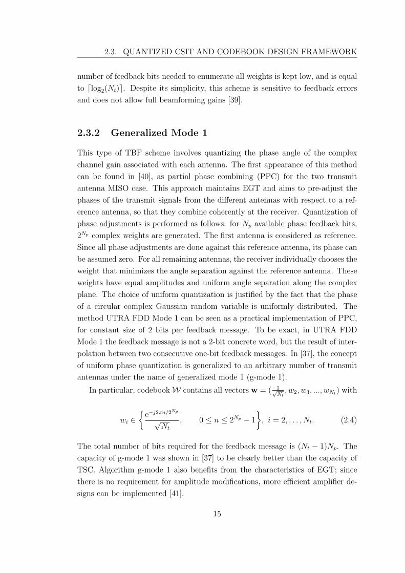
2.3.2 Generalized Mode 1 . . . . . . . . . . . . . . . . . . . . . . 15
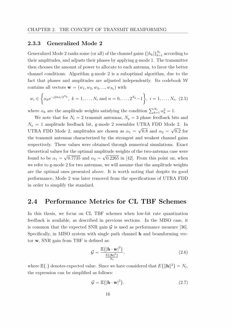
2.3.3 Generalized Mode 2 . . . . . . . . . . . . . . . . . . . . . . 16
2.4 Performance Metrics for CL TBF Schemes . . . . . . . . . . . . . 16
3 Interference Management in Two-tier HetNets 19
3.1 Open Access Control Mechanism for Femto Cells . . . . . . . . . 19
3.2 Power Control . . . . . . . . . . . . . . . . . . . . . . . . . . . . . 20
3.3 Resource Partitioning . . . . . . . . . . . . . . . . . . . . . . . . . 21
3.4 Successive Interference Cancellation . . . . . . . . . . . . . . . . . 23
3.5 Coordinated Multi-Point Transmission . . . . . . . . . . . . . . . 24
3.6 Altruistic Beamforming . . . . . . . . . . . . . . . . . . . . . . . . 25
4 Generalized System Model 29
4.1 Adopted Assumptions . . . . . . . . . . . . . . . . . . . . . . . . 29
ix
4.2 Mean and Instantaneous SINR at the MUE . . . . . . . . . . . . 31
4.3 System Parameters . . . . . . . . . . . . . . . . . . . . . . . . . . 32
4.4 Probabilistic Modeling of Instantaneous Received SINR . . . . . . 33
5 Perfect Phase Altruistic Beamforming 35
5.1 Received SINR with Unrestricted Phase Feedback Resolution . . . 36
5.2 Probability Distribution for Desired Signal . . . . . . . . . . . . . 38
5.3 Probability Distribution for Interfering Signal . . . . . . . . . . . 39
5.4 Cumulative Distribution Function of SINR . . . . . . . . . . . . . 39
6 Altruistic Beamforming in Multiple Interference Sources 43
6.1 Chi-squared Approximations for Desired and Interference Signals . 43
6.2 Egoistic TBF in all FBS Interferers . . . . . . . . . . . . . . . . . 45
6.3 Altruistic TBF only in Dominant FBS Interferer . . . . . . . . . . 45
6.4 Altruistic TBF in Multiple Dominant FBS Interferers . . . . . . . 45
6.4.1 Multiple Interferers with Different Mean Received Powers
at the MUE . . . . . . . . . . . . . . . . . . . . . . . . . . 46
6.4.2 Multiple Interferers with Equal Received Powers at the MUE 56
6.5 Performance Degradation at the FUE . . . . . . . . . . . . . . . . 58
7 Extensions of Altruistic Beamforming Methods 59
7.1 Increasing Amplitude Feedback Resolution . . . . . . . . . . . . . 59
7.2 Increasing the Number of Transmit Antennas . . . . . . . . . . . 64
8 Conclusions and Future Work 67
8.1 Conclusions . . . . . . . . . . . . . . . . . . . . . . . . . . . . . . 67
8.2 Future Work . . . . . . . . . . . . . . . . . . . . . . . . . . . . . . 68
Bibliography 71
Appendix A Perfect Phase Feedback: PDF of Egoistic Case 79
Appendix B Perfect Phase Feedback: Calculation of SINR 83
x
Chapter 1
Introduction
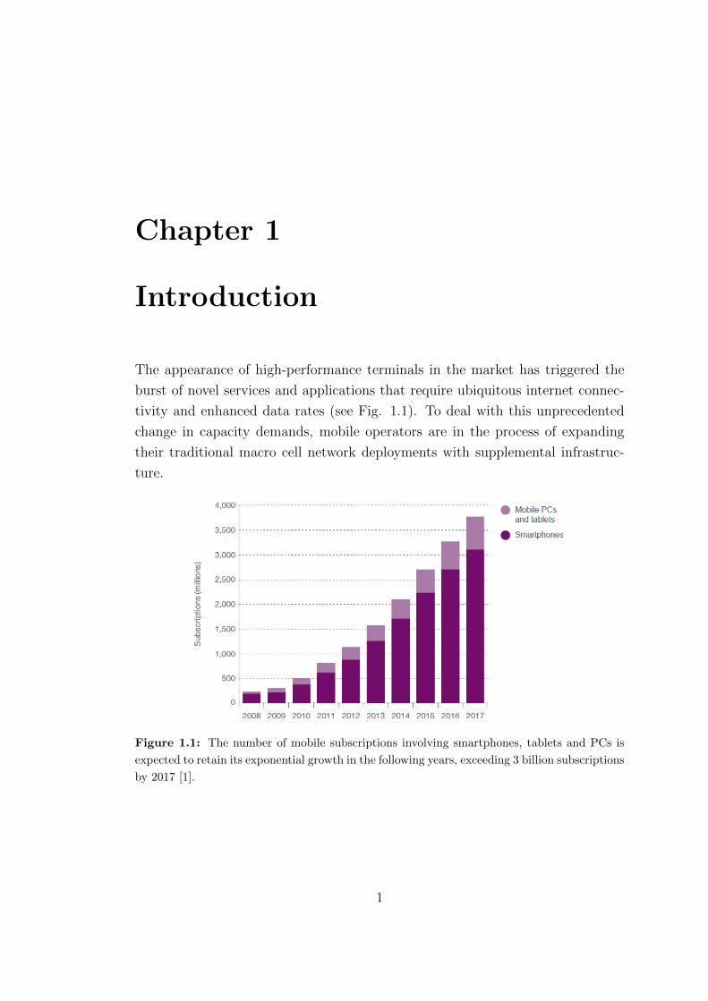
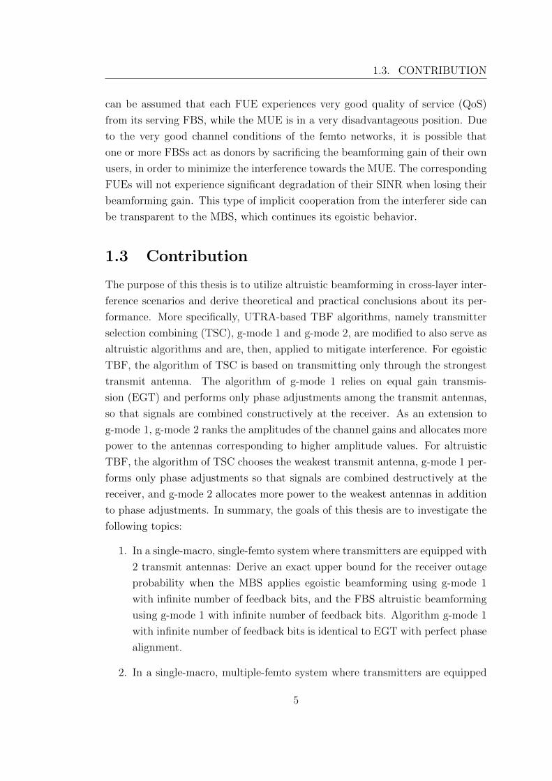
The appearance of high-performance terminals in the market has triggered the
burst of novel services and applications that require ubiquitous internet connec-
tivity and enhanced data rates (see Fig. 1.1). To deal with this unprecedented
change in capacity demands, mobile operators are in the process of expanding
their traditional macro cell network deployments with supplemental infrastruc-
ture.
Figure 1.1: The number of mobile subscriptions involving smartphones, tablets and PCs is
expected to retain its exponential growth in the following years, exceeding 3 billion subscriptions
by 2017 [1].
1
CHAPTER 1. INTRODUCTION
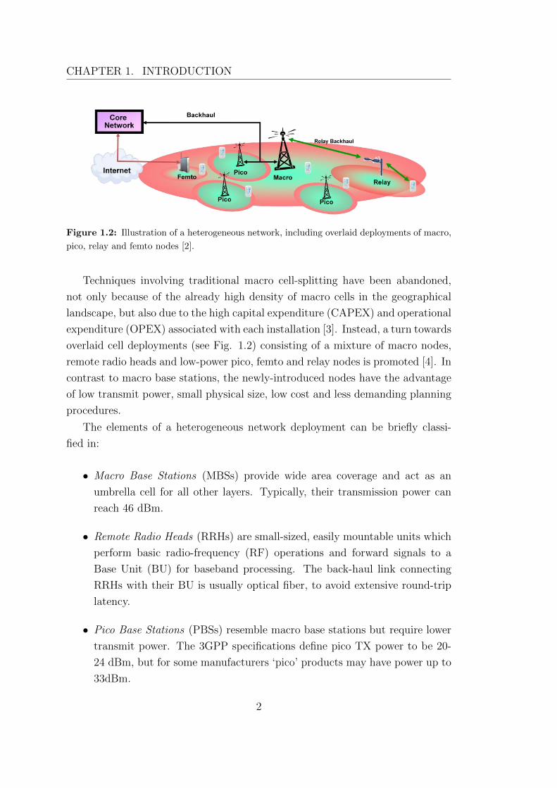
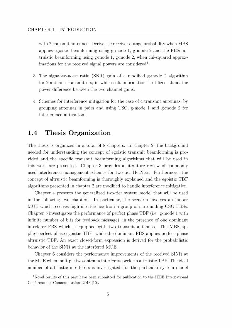
Figure 1.2: Illustration of a heterogeneous network, including overlaid deployments of macro,
pico, relay and femto nodes [2].
Techniques involving traditional macro cell-splitting have been abandoned,
not only because of the already high density of macro cells in the geographical
landscape, but also due to the high capital expenditure (CAPEX) and operational
expenditure (OPEX) associated with each installation [3]. Instead, a turn towards
overlaid cell deployments (see Fig. 1.2) consisting of a mixture of macro nodes,
remote radio heads and low-power pico, femto and relay nodes is promoted [4]. In
contrast to macro base stations, the newly-introduced nodes have the advantage
of low transmit power, small physical size, low cost and less demanding planning
procedures.
The elements of a heterogeneous network deployment can be briefly classi-
fied in:
• Macro Base Stations (MBSs) provide wide area coverage and act as an
umbrella cell for all other layers. Typically, their transmission power can
reach 46 dBm.
• Remote Radio Heads (RRHs) are small-sized, easily mountable units which
perform basic radio-frequency (RF) operations and forward signals to a
Base Unit (BU) for baseband processing. The back-haul link connecting
RRHs with their BU is usually optical fiber, to avoid extensive round-trip
latency.
• Pico Base Stations (PBSs) resemble macro base stations but require lower
transmit power. The 3GPP specifications define pico TX power to be 20-
24 dBm, but for some manufacturers ‘pico’ products may have power up to
33dBm.
2
1.1. MOTIVATION
• Relay Nodes (RNs) extend the wireless link between cell-edge users and
their serving MBS by acting as a pipeline [5].
• Femto Base Stations (FBSs) are plug-and-play indoor base stations (BSs)
that typically transmit with lower powers than 20 dBm [6]. Unlike all the
previously mentioned nodes, femto nodes are owned and installed individ-
ually by end users, therefore their exact placement cannot be planned by
the operator.
The presence of heterogeneous elements in the network provides flexibility in
site acquisition and lower total expenses for the operator, while it also promotes
seamless broadband experience for subscribers. Furthermore, from an environ-
mental point of view, it decreases unnecessary energy consumption. The most
important feature of a heterogeneous network (HetNet), though, is the capability
of simultaneous transmission over the same frequency bands, resulting in better
utilization of the limited spectrum resources available to the operator.
1.1 Motivation
A major concern for the success of HetNets is the handling of co-layer and
cross-layer interference. Co-layer interference is caused between nodes of the
same type, while cross-layer interference involves nodes which belong to different
tiers [6]. Usually, focus is given on cross-layer interference management sce-
narios involving macro and femto layers [7], due to the large power disparities
between the two layers, the opportunistic user-deployed nature of the FBSs and,
most importantly, the expected closed subscriber group (CSG) configuration for
FBSs, which results to dead coverage zones both in downlink and uplink. In the
downlink, CSG configuration forbids handover possibilities for a highly interfered
macro user equipment (MUE) which is in the vicinity of an FBS. Conversely, in
the uplink, the MUE is the source of interference and the victim is the nearby
FBS, which cannot easily separate the incoming signal from its associated femto
user equipment (FUE) from the interference. The work pursued in this thesis is
motivated by the above observations and aims to provide effective and efficient
solutions for dealing with the challenges of cross-layer interference.
3
CHAPTER 1. INTRODUCTION
1.2 Problem Context
Contemporary transmitters are equipped with multiple transmit antennas that
can be utilized to provide additional degrees of freedom for the transmission of
data. Transmit beamforming (TBF) [8] is a transmitter-side technique which uti-
lizes multiple antennas to enhance the reception quality of a single symbol at a
receiver equipped with a single receive antenna. In particular, TBF manipulates
the signals of all transmit antennas in such a way that coherent combining is
automatically performed at the target receiver. For TBF to work, it is vital that
channel state information is available at the transmitter (CSIT). In frequency
division duplex (FDD) systems, this can only be achieved through explicit feed-
back from the receiver, due to lack of reciprocity between downlink and uplink
channel responses. Typically, TBF is used in an egoistic manner, aiming to shape
signals of different antennas in such a way that they combine constructively at
the receiver. This pre-adjustment provides a so-called beamforming gain at the
receiver, since phases of the received signals are no longer random. Another
use of TBF is to mitigate the channel strength between an interferer and a vic-
tim user who suffers from the emitted interference. In that case, TBF shifts its
operation mode from egoistic to altruistic, aiming to shape the signals at the dif-
ferent antennas in such a way that they combine destructively at the victim user.
This change of behavior from the interfering transmitter reduces interference at
the victim user, but simultaneously sacrifices the beamforming gain previously
observed at the served user.
Altruistic beamforming is an interference mitigation technique that could per-
fectly fit in the context of cross-layer downlink interference in two-tier macro-
femto networks. Usually, in two-tier systems, the macro cell is modeled as pri-
mary infrastructure, since it promises ubiquitous coverage and is responsible for
serving a larger number of subscribers [9]. For this reason, higher priority is
commonly given to downlink interference scenarios, where the MUE is the vic-
tim. Indeed, consider the case where an MUE is in the vicinity of one or more
co-channel CSG femto cells that operate simultaneously. Immediately, the signal-
to-interference plus noise ratio (SINR) perceived by the MUE drops significantly,
due to the strong incoming FBS interference and the weakened signal from its
own MBS. On the other hand, it is typical that FUE operation benefits from the
slowly varying indoor environment, the small distance between FBS and FUE
and the presence of walls which act as a shield against outdoor signals. Thus, it
4
1.3. CONTRIBUTION
can be assumed that each FUE experiences very good quality of service (QoS)
from its serving FBS, while the MUE is in a very disadvantageous position. Due
to the very good channel conditions of the femto networks, it is possible that
one or more FBSs act as donors by sacrificing the beamforming gain of their own
users, in order to minimize the interference towards the MUE. The corresponding
FUEs will not experience significant degradation of their SINR when losing their
beamforming gain. This type of implicit cooperation from the interferer side can
be transparent to the MBS, which continues its egoistic behavior.
1.3 Contribution
The purpose of this thesis is to utilize altruistic beamforming in cross-layer inter-
ference scenarios and derive theoretical and practical conclusions about its per-
formance. More specifically, UTRA-based TBF algorithms, namely transmitter
selection combining (TSC), g-mode 1 and g-mode 2, are modified to also serve as
altruistic algorithms and are, then, applied to mitigate interference. For egoistic
TBF, the algorithm of TSC is based on transmitting only through the strongest
transmit antenna. The algorithm of g-mode 1 relies on equal gain transmis-
sion (EGT) and performs only phase adjustments among the transmit antennas,
so that signals are combined constructively at the receiver. As an extension to
g-mode 1, g-mode 2 ranks the amplitudes of the channel gains and allocates more
power to the antennas corresponding to higher amplitude values. For altruistic
TBF, the algorithm of TSC chooses the weakest transmit antenna, g-mode 1 per-
forms only phase adjustments so that signals are combined destructively at the
receiver, and g-mode 2 allocates more power to the weakest antennas in addition
to phase adjustments. In summary, the goals of this thesis are to investigate the
following topics:
1. In a single-macro, single-femto system where transmitters are equipped with
2 transmit antennas: Derive an exact upper bound for the receiver outage
probability when the MBS applies egoistic beamforming using g-mode 1
with infinite number of feedback bits, and the FBS altruistic beamforming
using g-mode 1 with infinite number of feedback bits. Algorithm g-mode 1
with infinite number of feedback bits is identical to EGT with perfect phase
alignment.
2. In a single-macro, multiple-femto system where transmitters are equipped
5
CHAPTER 1. INTRODUCTION
with 2 transmit antennas: Derive the receiver outage probability when MBS
applies egoistic beamforming using g-mode 1, g-mode 2 and the FBSs al-
truistic beamforming using g-mode 1, g-mode 2, when chi-squared approx-
imations for the received signal powers are considered1.
3. The signal-to-noise ratio (SNR) gain of a modified g-mode 2 algorithm
for 2-antenna transmitters, in which soft information is utilized about the
power difference between the two channel gains.
4. Schemes for interference mitigation for the case of 4 transmit antennas, by
grouping antennas in pairs and using TSC, g-mode 1 and g-mode 2 for
interference mitigation.
1.4 Thesis Organization
The thesis is organized in a total of 8 chapters. In chapter 2, the background
needed for understanding the concept of egoistic transmit beamforming is pro-
vided and the specific transmit beamforming algorithms that will be used in
this work are presented. Chapter 3 provides a literature review of commonly
used interference management schemes for two-tier HetNets. Furthermore, the
concept of altruistic beamforming is thoroughly explained and the egoistic TBF
algorithms presented in chapter 2 are modified to handle interference mitigation.
Chapter 4 presents the generalized two-tier system model that will be used
in the following two chapters. In particular, the scenario involves an indoor
MUE which receives high interference from a group of surrounding CSG FBSs.
Chapter 5 investigates the performance of perfect phase TBF (i.e. g-mode 1 with
infinite number of bits for feedback message), in the presence of one dominant
interferer FBS which is equipped with two transmit antennas. The MBS ap-
plies perfect phase egoistic TBF, while the dominant FBS applies perfect phase
altruistic TBF. An exact closed-form expression is derived for the probabilistic
behavior of the SINR at the interfered MUE.
Chapter 6 considers the performance improvements of the received SINR at
the MUE when multiple two-antenna interferers perform altruistic TBF. The ideal
number of altruistic interferers is investigated, for the particular system model
1Novel results of this part have been submitted for publication to the IEEE International
Conference on Communications 2013 [10].
6

1.4. THESIS ORGANIZATION
and scenario. In chapter 7, schemes that expand the performance of altruistic
TBF algorithms are investigated. Finally, in chapter 8, conclusions are presented
and possible future research directions to extend this work are also suggested.
7

CHAPTER 1. INTRODUCTION
8
Chapter 2
The Concept of Transmit
Beamforming
Multiple antennas at the receiver can coherently combine the received signal
paths so that the effects of the fading channel are alleviated, without the need
for increased transmit power or bandwidth. Multiple antennas at the trans-
mitter can also be exploited to enhance the received SNR of the served user,
particularly in the downlink direction. Improvements in performance can be
high, especially when using feedback schemes to provide the transmitter with
knowledge of the channel response. With that knowledge, the transmitter can
apply precoding techniques to shape its transmit symbols so that the instan-
taneous effect of the channel is mitigated. In this thesis, we will consider the
multiple input single output (MISO) model; therefore, instead of ‘precoding’, the
term ‘transmit beamforming’ will be used. The difference is that precoding is
linked with MIMO systems and involves sending multiple data streams spatially
through independent eigen-channels, while transmit beamforming implies single-
layer transmission [8].
2.1 Classification of Transmit Diversity Meth-
ods
Transmit diversity utilizes the presence of multiple antennas at the transmitter in
order to enhance the quality of the signal at the receiver side. Transmit diversity
schemes have been mostly attractive for the downlink direction, since complexity
issues (e.g. cost, power, space, processing) can be more easily managed at the BS
9
CHAPTER 2. THE CONCEPT OF TRANSMIT BEAMFORMING
side. In general, transmit diversity modes are classified as open-loop (OL) and
closed-loop (CL). This categorization stems from the fact that the former do not
require the presence of CSIT, while the latter cannot function without it.
2.1.1 Channel State Information at the Transmitter Side
Unlike the receiver, the transmitter does not always have direct access to channel
fading information. In principle, there are two possible methods of acquiring
CSIT; in time division duplex (TDD) systems, CSIT can be obtained directly
from estimation of the uplink channel (open-loop channel acquisition), while in
FDD systems, the receiver is responsible for sending back information about the
channel, due to lack of reciprocity between downlink and uplink (closed-loop
channel acquisition) [11]. Presence of CSIT is considered critical for maximizing
the achievable rates for users of the system. Despite its advantages, assuming
complete CSIT is unrealistic, due to the uncertainty of the wireless medium and
complications in CSIT acquisition.
2.1.2 Open-Loop Methods
In OL systems, the transmitter does not require knowledge of the channel. There-
fore, such techniques do not depend on control information fed back by the re-
ceiver. In general, OL methods are favored against CL ones in situations in-
volving high mobility or limitations in feedback capability. Different OL meth-
ods for multi-antenna systems have been proposed through the years, among
which are Delay Transmit Diversity (DTD) [12], Orthogonal Transmit Diversity
(OTD) [13], Space Time Spreading (STS) [14], Phase Sweep Transmit Diversity
(PSTD) [15], Time Switched Transmit Diversity (TSTD) [16] and Space-time
Transmit Diversity (STTD) [17]. Probably the most commonly noted OL method
is the simple Alamouti scheme [18], which is based on STTD and achieves a di-
versity order of two, the highest possible for a two transmit antenna system. Pre-
sentation and comparison of OL techniques incorporated in 3rd generation (3G)
systems can be found in [19][20]. A brief description of OL techniques for long
term evolution (LTE) can be found in [21].
10
2.2. TRANSMIT BEAMFORMING AND MISO SYSTEM MODEL
2.1.3 Closed-Loop Methods
In CL systems, the transmitter requires knowledge of the channel. In such sys-
tems, the receiver has the capability to periodically measure the channel and re-
port back to the transmitter, through a specified control channel, information that
will help to improve the perceived performance. In general, channel knowledge
acquired at the transmitter is imperfect, due to the error-prone, delay-sensitive
and capacity-limited nature of the feedback channel.
Extensive research has been carried out for finding efficient ways to convey
and optimally utilize partial CSIT through the available control channel. Partial
feedback strategies presented in literature typically focus on different character-
istics of the real-time feedback channel separately for simplicity. As an example,
mean and covariance feedback models [22][23][24] focus on the effects of feedback
delay and channel estimation errors, but usually assume that mean and covariance
values are fed back in non-quantized form. Similarly, magnitude feedback, which
involves sending back information only about the norm of the channel gains [25],
assumes that accurate values of the channel norm can be fed back.
From a different perspective, quantized feedback schemes [26][27][28][29][30]
are based on the realization that feedback channel capacity is limited. With
limited channel capacity for signaling purposes, the design goal of the system
is to minimize the uplink overhead and optimize a performance metric at the
receiver (e.g. received SNR). Effectiveness of quantized CL feedback schemes
depends on the availability, accuracy and update rate of CSIT. Thus, trade-offs
between resolution and frequency of feedback must be considered. It has been
verified that in fast fading channels, the most critical factor is the frequency of
feedback, while in slow-fading channels priority should be given to the resolution
of feedback [31].
2.2 Transmit Beamforming and MISO System
Model
Transmit beamforming is a processing technique that exploits knowledge of CSIT
to optimally adapt the transmit symbols to channel conditions, and enhance
performance at the receiver side by altering the transmission radiation pattern.
The term ‘transmit beamforming’ commonly represents a special case of precoding
(i.e. single-layer precoding) and can be easiest described using a MISO system
11
CHAPTER 2. THE CONCEPT OF TRANSMIT BEAMFORMING
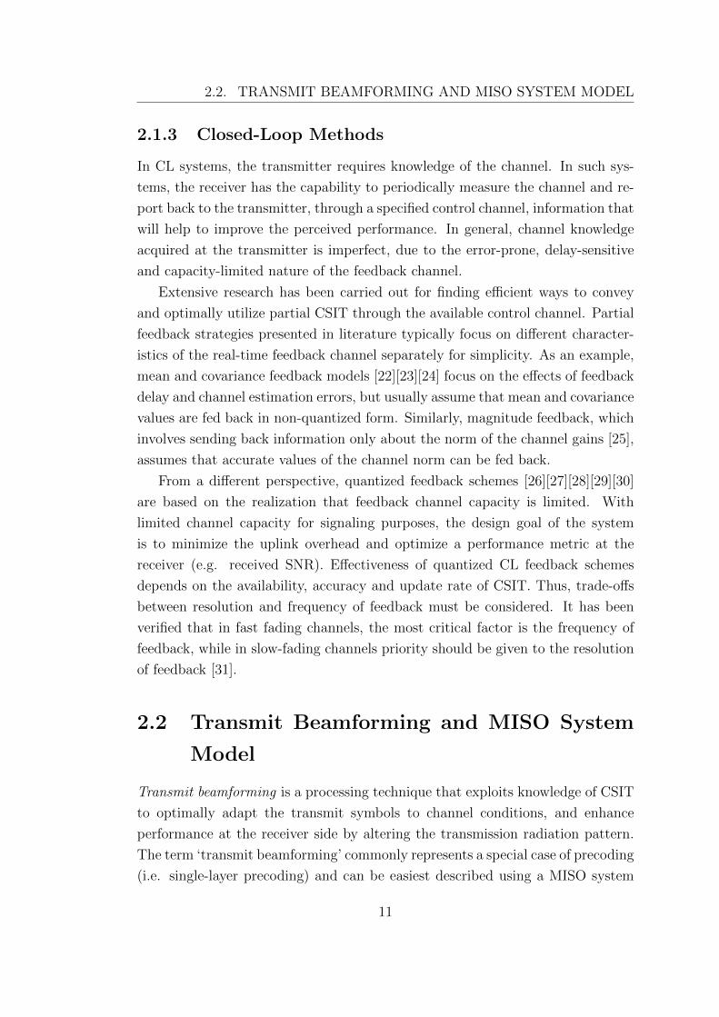
Figure 2.1: Transmit beamforming block diagram. Symbol s is sent through Nt transmit
antennas. Prior to transmission, a beamforming weight wi is applied to the signal of each
antenna, according to knowledge obtained from the receiver, through a finite rate feedback
channel. At the receiver, the signal y is received.
model. With TBF, a single symbol s is sent through n of the available Nt transmit
antennas (n ≤Nt) after it has been multiplied by a beamforming vector w (see
Fig. 2.1). The vector channel h consists of scalar complex weights hi, each
corresponding to the channel between the i-th transmit antenna and the receiver.
The beamforming vector w consists of scalar complex weights wi, which are
chosen based on the feedback information acquired by the receiver. Beamforming
vectors need to satisfy ‖w‖ ≤ 1, so that amplifications in the available transmit
power are avoided. At the single-antenna receiver, the signal y is received, which
is the superposition of the signals from all transmit antennas.
We will assume that the BS is equipped with Nt transmit antennas and the
user equipment (UE) with a single receive antenna. Considering single path
Rayleigh fading channels, the vector channel is given by h = [h1, h2, ..., hNt ],
where hi are independent and identically distributed (i.i.d.) zero-mean circularly
symmetric complex Gaussian random variables (RVs) normalized to unit power.
With E{|hi|2} = 1, we have E{‖h‖2} = Nt. Let w = [w1, w2, ..., wNt ], with
‖w‖ = 1, be the chosen beamforming vector from a predefined codebook W . For
conventional TBF, the goal is to maximize SNR at reception (i.e. egoistic TBF),
12
2.3. QUANTIZED CSIT AND CODEBOOK DESIGN FRAMEWORK
thus, w is chosen such that
w = arg maxw∈W|h ·w|. (2.1)
Then, the received signal at the target UE is
y = (h · w)s+ n, (2.2)
where n ∈ C is zero-mean complex Gaussian noise with noise spectral density N0.
2.3 Quantized CSIT and Codebook Design Frame-
work
Perfect knowledge of CSIT is unrealistic in practical systems. Hence, the choice
of w is based on quantized information fed back by the receiver at periodic
time intervals. In early works [32][33], the receiver quantized the channel itself,
and directly designed the optimal beamforming vector to be fed back to the
transmitter. It is evident that the performance of such an approach is bounded,
since it depends on resolution, which cannot be infinite due to limitations of the
feedback channel. A simpler approach is to quantize the set of beamforming
vectors, not their actual values. The set of chosen beamforming vectors forms
a codebook W , which can be shared among transmitter and receiver prior to
transmission. Then, the receiver only needs to send back to the transmitter the
index of the beamforming vector that maximizes performance. Typically, the CL
procedure for this type of TBF is the following:
1. The receiver, at each time instant, selects the optimal beamforming vec-
tor w from a pre-defined codebook W , with goal to maximize some perfor-
mance metric.
2. The receiver feeds back the index of the chosen beamforming vector.
3. The transmitter retrieves the actual beamforming vector, corresponding to
the index received, from its own copy of codebook W and applies it for
transmission.
Generalized techniques for the design of transmit beamforming codebooks
have been proposed in literature through the years. One approach is to think
of codebook W as a collection of lines in the Euclidean CNt space and try to
13
CHAPTER 2. THE CONCEPT OF TRANSMIT BEAMFORMING
maximize the angular separation among the closest neighboring lines [34]. This
formulation of the solution is identical to the well-known Grassmanian line pack-
ing problem of applied mathematics. A second approach is to build codebooks
by using vector quantization (VQ) techniques. The idea of VQ is based on max-
imizing the mean-squared weighted inner product between the optimum and the
quantized beamforming vector [35]. The previous techniques assume that code-
books are deterministic and independent of the channel conditions. Random
Vector Quantization (RVQ), on the other hand, relies on random codebook gen-
eration after each channel fading block. These random codebooks must be known
perfectly at both transmitter and receiver. Assuming NB feedback bits, RVQ gen-
erates 2NB codebook vectors i.i.d. according to the stationary distribution of the
best unquantized beamforming vector. A survey of the various codebook design
techniques can be found in [8].
Practical CL systems use simple deterministic codebooks that require low
overhead. Wideband code division multiple access (WCDMA) was the first mo-
bile system that contained explicit support for CL transmit beamforming meth-
ods. Incorporation to the standard was based on the observation that, even
with minimal quantized feedback resolution, performance improvements were no-
ticeable [36]. In our analysis, we will consider the generalized UTRA-based CL
transmit diversity modes found in [37], namely transmitter selection combining
(TSC), generalized mode-1 (g-mode 1) and generalized mode-2 (g-mode 2). The
codebooks of these modes do not comply with optimal codebook design, but the
performance loss is negligible compared to more complex designs [26][34] for small
number of transmit antennas and implementation is straightforward [37].
2.3.1 Transmitter Selection Combining
The simplest codebook design technique is TSC, also referred to as selection
diversity transmission (SDT) or transmit antenna selection (TAS) [38]. In this
feedback scheme, the beamforming vector contains only one non-zero entry. The
only non-zero entry corresponds to the transmit antenna that maximizes the
received SNR. Hence, codebook W has the following form:
W = {(0, ..., 0, 1i, 0, ..., 0), i = 1, . . . , Nt}, (2.3)
where i indicates the position of the non-zero value in the vector. The size of this
codebook is equal to the number of available transmit antennas Nt; therefore, the
14
2.3. QUANTIZED CSIT AND CODEBOOK DESIGN FRAMEWORK
number of feedback bits needed to enumerate all weights is kept low, and is equal
to dlog2(Nt)e. Despite its simplicity, this scheme is sensitive to feedback errors
and does not allow full beamforming gains [39].
2.3.2 Generalized Mode 1
This type of TBF scheme involves quantizing the phase angle of the complex
channel gain associated with each antenna. The first appearance of this method
can be found in [40], as partial phase combining (PPC) for the two transmit
antenna MISO case. This approach maintains EGT and aims to pre-adjust the
phases of the transmit signals from the different antennas with respect to a ref-
erence antenna, so that they combine coherently at the receiver. Quantization of
phase adjustments is performed as follows: for Np available phase feedback bits,
2Np complex weights are generated. The first antenna is considered as reference.
Since all phase adjustments are done against this reference antenna, its phase can
be assumed zero. For all remaining antennas, the receiver individually chooses the
weight that minimizes the angle separation against the reference antenna. These
weights have equal amplitudes and uniform angle separation along the complex
plane. The choice of uniform quantization is justified by the fact that the phase
of a circular complex Gaussian random variable is uniformly distributed. The
method UTRA FDD Mode 1 can be seen as a practical implementation of PPC,
for constant size of 2 bits per feedback message. To be exact, in UTRA FDD
Mode 1 the feedback message is not a 2-bit concrete word, but the result of inter-
polation between two consecutive one-bit feedback messages. In [37], the concept
of uniform phase quantization is generalized to an arbitrary number of transmit
antennas under the name of generalized mode 1 (g-mode 1).
In particular, codebookW contains all vectors w = ( 1√Nt, w2, w3, ..., wNt) with
wi ∈{
e−j2πn/2Np
√Nt
, 0 ≤ n ≤ 2Np − 1
}, i = 2, . . . , Nt. (2.4)
The total number of bits required for the feedback message is (Nt − 1)Np. The
capacity of g-mode 1 was shown in [37] to be clearly better than the capacity of
TSC. Algorithm g-mode 1 also benefits from the characteristics of EGT; since
there is no requirement for amplitude modifications, more efficient amplifier de-
signs can be implemented [41].
15
CHAPTER 2. THE CONCEPT OF TRANSMIT BEAMFORMING
2.3.3 Generalized Mode 2
Generalized Mode 2 ranks some (or all) of the channel gains {|hk|}Ntk=1 according to
their amplitudes, and adjusts their phases by applying g-mode 1. The transmitter
then chooses the amount of power to allocate to each antenna, to favor the better
channel conditions. Algorithm g-mode 2 is a suboptimal algorithm, due to the
fact that phases and amplitudes are adjusted independently. Its codebook Wcontains all vectors w = (w1, w2, w3, ..., wNt) with
wi ∈{αke
−j2πn/2Np , k = 1, . . . , Nt and n = 0, . . . , 2Np−1
}, i = 1, . . . , Nt, (2.5)
where αk are the amplitude weights satisfying the condition∑Nt
k=1 α2k = 1.
We note that for Nt = 2 transmit antennas, Np = 3 phase feedback bits and
Na = 1 amplitude feedback bit, g-mode 2 resembles UTRA FDD Mode 2. In
UTRA FDD Mode 2, amplitudes are chosen as α1 =√
0.8 and α2 =√
0.2 for
the transmit antennas characterized by the strongest and weakest channel gains
respectively. These values were obtained through numerical simulations. Exact
theoretical values for the optimal amplitude weights of the two-antenna case were
found to be α1 =√
0.7735 and α2 =√
0.2265 in [42]. From this point on, when
we refer to g-mode 2 for two antennas, we will assume that the amplitude weights
are the optimal ones presented above. It is worth noting that despite its good
performance, Mode 2 was later removed from the specifications of UTRA FDD
in order to simplify the standard.
2.4 Performance Metrics for CL TBF Schemes
In this thesis, we focus on CL TBF schemes when low-bit rate quantization
feedback is available, as described in previous sections. In the MISO case, it
is common that the expected SNR gain G is used as performance measure [36].
Specifically, in MISO system with single path channel h and beamforming vec-
tor w, SNR gain from TBF is defined as:
G =E{|h ·w|2}
E{‖h‖2}Nt
, (2.6)
where E{.} denotes expected value. Since we have considered that E{‖h‖2} = Nt,
the expression can be simplified as follows:
G = E{|h ·w|2}. (2.7)
16
2.4. PERFORMANCE METRICS FOR CL TBF SCHEMES
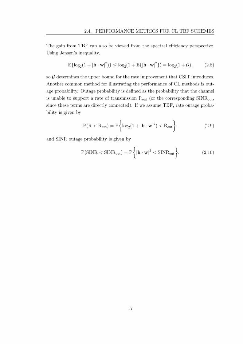
The gain from TBF can also be viewed from the spectral efficiency perspective.
Using Jensen’s inequality,
E{log2(1 + |h ·w|2)} ≤ log2(1 + E{|h ·w|2}) = log2(1 + G), (2.8)
so G determines the upper bound for the rate improvement that CSIT introduces.
Another common method for illustrating the performance of CL methods is out-
age probability. Outage probability is defined as the probability that the channel
is unable to support a rate of transmission Rout (or the corresponding SINRout,
since these terms are directly connected). If we assume TBF, rate outage proba-
bility is given by
P(R < Rout) = P
{log2(1 + |h ·w|2) < Rout
}, (2.9)
and SINR outage probability is given by
P(SINR < SINRout) = P
{|h ·w|2 < SINRout
}. (2.10)
17

CHAPTER 2. THE CONCEPT OF TRANSMIT BEAMFORMING
18
Chapter 3
Interference Management in
Two-tier HetNets
The shift towards overlaid co-channel network deployments has introduced fur-
ther challenges in the management of interference present in future networks.
Various techniques have been proposed for limiting the effect of cross-layer inter-
ference. The most important interference management schemes include open ac-
cess mechanism for FBSs, power control for FBSs, resource partitioning between
different layers, advanced receivers with interference cancellation capabilities, co-
operative transmissions between geographically separated BSs and multi-antenna
techniques.
3.1 Open Access Control Mechanism for Femto
Cells
Open access mechanism for femto cells is usually disregarded in heterogeneous
scenario modeling due to security reasons, limited backhaul bandwidth and shar-
ing concerns of owners. Despite its low popularity, the presence of open access
FBSs would immediately alleviate most of the interference problems that accom-
pany closed access. Theoretical studies [43] have shown that open access does
not pose a negative impact on the interference conditions of a heterogeneous net-
work, when compared to conventional macro single-layer deployments. In fact,
it is deduced that network capacity can increase linearly when open access FBSs
are deployed in multi-tier networks. In [44], the dominance of open against closed
access is highlighted through simulations, which illustrate that open access can
19
CHAPTER 3. INTERFERENCE MANAGEMENT IN TWO-TIERHETNETS
boost the total cell throughput by 15 % compared to closed access. The observed
results can be justified intuitively. With open access, users would simply hand
over their connections to the strongest base station and no dead zones would be
created. As a consequence, the new optimal connections would lower the trans-
mission powers for the uplink and downlink directions in all base stations of the
multi-tier network. All these advantages would come at the cost of the extra
signaling, and the possible reduction in the performance of the femto cell user,
since resources would no longer be dedicated [45].
3.2 Power Control
Deployment of femto cells in CSG access method under co-channel operation with
the macro cell causes coverage holes in the macro layer. Several downlink power
control (PC) mechanisms have been investigated to combat the presence of dead
coverage zones, mainly through adjustments of the transmit powers at the FBS,
either in a fixed or dynamic way [46]. The basic requirement is to limit the femto
coverage so that interference towards macro users is decreased, but at the same
time performance at the served femto UEs is not devastated.
Typically, FBSs set their transmit power after initial start-up, by sensing the
surrounding RF conditions, such as the neighbor FBSs list or the macro cell
coverage. Fixing the FBS node transmit power to its maximum allowed value
is not considered a good option and has already been disregarded [46]. In that
particular technical report, it is proposed that the FBS transmit power should
be settable from the maximum capable value down to a level of 0 dBm. This
procedure can even be assisted by global positioning system (GPS) receivers in
the FBS, through a mapping between maximum transmit power and number of
detected satellites or reception quality [47]. More specifically, if the FBS is unable
to detect a sufficient number of satellites, it can be deduced that it is well within
the building area and, thus, well isolated. Then, it can set its transmit power to
a higher level and still not pose a significant threat to MUEs lying outside the
building.
In general, it has been shown that fixed power does not provide good results
in all deployment scenarios, and that adaptive calibration of the transmit power
should be considered [7]. Calibration of FBS transmit power provides a method
to adaptively modify femto coverage, depending on the macro cell interference
levels [48]. The algorithm behind power calibration is based on measurements
20
3.3. RESOURCE PARTITIONING
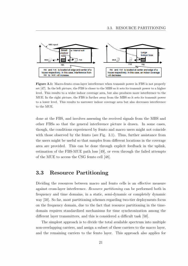
Figure 3.1: Macro-femto cross-layer interference when transmit power in FBS is not properly
set [47]. In the left picture, the FBS is closer to the MBS so it sets its transmit power to a higher
level. This results to a wider indoor coverage area, but also produces more interference to the
MUE. In the right picture, the FBS is further away from the MBS so it sets its transmit power
to a lower level. This results to narrower indoor coverage area but also decreases interference
to the MUE.
done at the FBS, and involves assessing the received signals from the MBS and
other FBSs so that the general interference picture is drawn. In some cases,
though, the conditions experienced by femto and macro users might not coincide
with those observed by the femto (see Fig. 3.1). Thus, further assistance from
the users might be useful so that samples from different locations in the coverage
area are provided. This can be done through explicit feedback in the uplink,
estimation of the FBS-MUE path loss [49], or even through the failed attempts
of the MUE to access the CSG femto cell [48].
3.3 Resource Partitioning
Dividing the resources between macro and femto cells is an effective measure
against cross-layer interference. Resource partitioning can be performed both in
frequency and time domains, in a static, semi-dynamic or completely dynamic
way [50]. So far, most partitioning schemes regarding two-tier deployments focus
on the frequency domain, due to the fact that resource partitioning in the time-
domain requires standardized mechanisms for time synchronization among the
different layer transmitters, and this is considered a difficult task [50].
The simplest approach is to divide the total available spectrum into multiple
non-overlapping carriers, and assign a subset of these carriers to the macro layer,
and the remaining carriers to the femto layer. This approach also applies for
21
CHAPTER 3. INTERFERENCE MANAGEMENT IN TWO-TIERHETNETS
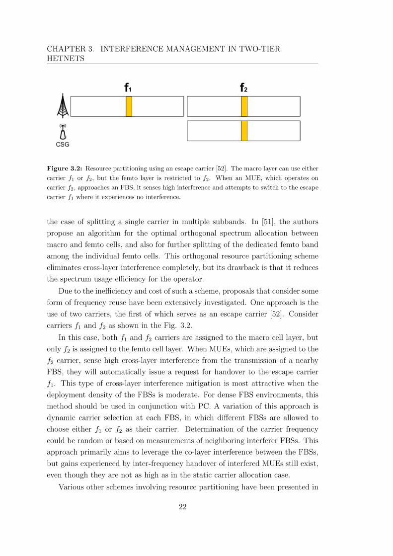
Figure 3.2: Resource partitioning using an escape carrier [52]. The macro layer can use either
carrier f1 or f2, but the femto layer is restricted to f2. When an MUE, which operates on
carrier f2, approaches an FBS, it senses high interference and attempts to switch to the escape
carrier f1 where it experiences no interference.
the case of splitting a single carrier in multiple subbands. In [51], the authors
propose an algorithm for the optimal orthogonal spectrum allocation between
macro and femto cells, and also for further splitting of the dedicated femto band
among the individual femto cells. This orthogonal resource partitioning scheme
eliminates cross-layer interference completely, but its drawback is that it reduces
the spectrum usage efficiency for the operator.
Due to the inefficiency and cost of such a scheme, proposals that consider some
form of frequency reuse have been extensively investigated. One approach is the
use of two carriers, the first of which serves as an escape carrier [52]. Consider
carriers f1 and f2 as shown in the Fig. 3.2.
In this case, both f1 and f2 carriers are assigned to the macro cell layer, but
only f2 is assigned to the femto cell layer. When MUEs, which are assigned to the
f2 carrier, sense high cross-layer interference from the transmission of a nearby
FBS, they will automatically issue a request for handover to the escape carrier
f1. This type of cross-layer interference mitigation is most attractive when the
deployment density of the FBSs is moderate. For dense FBS environments, this
method should be used in conjunction with PC. A variation of this approach is
dynamic carrier selection at each FBS, in which different FBSs are allowed to
choose either f1 or f2 as their carrier. Determination of the carrier frequency
could be random or based on measurements of neighboring interferer FBSs. This
approach primarily aims to leverage the co-layer interference between the FBSs,
but gains experienced by inter-frequency handover of interfered MUEs still exist,
even though they are not as high as in the static carrier allocation case.
Various other schemes involving resource partitioning have been presented in
22
3.4. SUCCESSIVE INTERFERENCE CANCELLATION
the academic and industrial literature. In [53], the direction of arrival (DoA) of
the MUE is compared to the direction range of the FBS, and the result determines
the type of scheduling that will be used. If the MUE is not in the direction range
of the FBS, it can use any of the available frequencies. Otherwise, the scheduling
priority of the frequency resources used by the FBS is set to a lower value, in order
to decrease the cross-layer interference towards the MUE. In [54], the macro cell
layer frequency resources are partitioned into contiguous non-overlapping sub-
bands under the fractional frequency reuse scheme (FFR), in which one subband
is assigned to the cell center zone and the remaining subbands are assigned to the
cell edge zone. The center band adopts a reuse factor of one, while the edge bands
adopt a larger reuse factor. For each subband, a different macro transmit power
is chosen. The claim of [54] is that such subband partitioning not only improves
the rates of the macro cell users, but also provides opportunities for simultaneous
femto cell transmissions through the same frequency resources, without emission
of extensive interference to the macro cell layer. In [55], the MBS senses when a
served MUE is in the vicinity of a high-interference femto cell and it dynamically
determines a set of resources that the FBS should restrict its transmission to.
This restriction message is then relayed through the MUE to the interferer FBS.
3.4 Successive Interference Cancellation
Successive interference cancellation (SIC) techniques have already been imple-
mented in 3G systems, and aim to exploit the structure of the interference through
reconstruction of the dominant interference signals and subtraction from the total
interference [56]. With SIC, the dominant interferer is the first to be detected
and decoded, due to its high received power when compared to the remaining
interfering signals. Using accurate channel gain estimation, the decoded version
of the interfering signal is regenerated in such a way that it resembles the actual
received signal, and is then subtracted from the composite received signal. This
procedure can be repeated for the remaining interferers. After each step, the
next user to be decoded faces less and less interference. Usage of SIC alone is
not as effective in heterogeneous deployments, due to differences in cross-layer
synchronization and opportunistic placements of femto nodes [57].
23
CHAPTER 3. INTERFERENCE MANAGEMENT IN TWO-TIERHETNETS
3.5 Coordinated Multi-Point Transmission
Recently, a lot of emphasis has been given on so-called coordinated transmis-
sion methods that could minimize inter-cell interference. Coordinated Multi-point
(CoMP) [58][59][60] is a technique, incorporated in 3GPP LTE-Advanced, whose
purpose is to exploit or avoid co-channel interference and enhance primarily cell-
edge user throughput between MBSs. Improving the signal strength at cell edge
implies improving the interference situation of the whole two-tier deployment.
Downlink CoMP strategies require the cooperation of geographically sepa-
rated base stations, for determining the transmission scheme that will jointly
optimize performance among their corresponding UEs. In CoMP, procedures of
beamforming, scheduling and data transmission are performed jointly in an ex-
plicit manner between collaborating nodes. Architectures of CoMP can be either
1. centralized or
2. distributed,
depending on how UE feedback is shared among the transmission points. Both
architectures support two schemes for the coordination of the transmission points;
for downlink, CoMP schemes are divided into
1. Joint Processing (JP) and
2. Cooperative Scheduling/Beamforming (CS/CB).
Centralized architecture demands the presence of a central unit (CU), which is re-
sponsible for gathering and processing CSIT information from all individual UEs
served by a cluster of cooperating MBSs. The cooperating MBSs are connected
to the CU in star topology via low-latency backhaul links, such as optical fiber.
These links carry signaling overhead and allow the cluster of MBSs to behave as
a single entity. Assuming FDD operation, UEs need to estimate CSIT informa-
tion regarding each MBS of the coordination cluster and report it to their own
serving (anchor) MBS. Each anchor MBS forwards the information received to
the central unit. Thus, global CSIT is only available at the CU. The CU jointly
processes the received CSI information to decide the scheduling of users and the
precoding parameters that each MBS should use. Finally, the CU forwards to
each MBS the chosen precoding parameters and transmission begins.
Distributed architecture was proposed in [61] to alleviate the challenges present
in the centralized architecture. In distributed architecture, the CU is completely
24
3.6. ALTRUISTIC BEAMFORMING
removed and backhaul links that connect MBSs are not necessary, since there is
no need for direct exchange of signaling or data information among MBSs any-
more. The benefit of a distributed approach is that deployment does not stray
too much from that of conventional systems, so only minimal changes are re-
quired for adaptation. The simplification of the architecture introduces changes
in the framework. Firstly, UEs do not send feedback only to their anchor MBS,
but to each MBS of the coordination cluster. Secondly, the burden of scheduling
and precoding is shifted to each MBS. Thus, it is important that the scheduling
algorithms, which are performed independently at each MBS, are identical.
In JP, data towards a UE is shared among the cooperating MBSs. This scheme
exploits the low correlation of the geographically separated sites to improve the
data transmission. Transmission can be either coherent or non-coherent, depend-
ing on whether phase information feedback is available to combine the signals
at the receiver or in an opportunistic way. Joint processing offers two different
approaches for transmission of data. With joint transmission (JT), data trans-
mission can be performed simultaneously by multiple MBSs. With dynamic cell
selection (DCS), fast dynamic scheduling is executed, usually on a subframe-per-
subframe basis, and a single MBS is chosen to transmit data. This MBS can be
different from the anchor MBS of the UE. Schemes based on JP can offer large
performance gains, particularly for cell-edge users.
In CS/CB, only the anchor MBS has access to data of its served UE. This
scheme requires coordination of user scheduling and beamforming among the
MBSs of the cluster in order to enhance sum data rates and reduce interference.
Theoretically, CS/CB is always outperformed by JP, since the former aims to
avoid interference while the latter exploits interference and converts it to useful
signal. When the capacity limit of the backhaul is taken into account, though, it
has been observed that CS/CB can produce better results than JP [62]. A more
thorough presentation of CoMP architectures and transmission schemes can be
found in [61][63][64][65].
3.6 Altruistic Beamforming
Altruistic Beamforming is a technique, first presented in [66], which boosts the
performance of a badly interfered UE by borrowing degrees of freedom from a
subset of its interferers. Although this technique was presented in the context of
co-layer femto interference, it can be directly adopted to cross-layer interference
25
CHAPTER 3. INTERFERENCE MANAGEMENT IN TWO-TIERHETNETS
scenarios involving a highly interfered MUE and multiple FBS interferers. Altruis-
tic beamforming can be utilized in downlink cross-layer interference scenarios that
involve an MUE located in the vicinity of multiple FBSs, which operate simulta-
neously with fixed transmit power. Initially, it is assumed that all transmitters
apply transmit beamforming in an egoistic manner, having as goal to maximize
the perceived rates of their own users. This results to severe degradation of the
SINR received at the MUE. In order to decrease the received cross-layer inter-
ference, the MUE establishes a control connection with a subset of its dominant
interferers and proposes that they change their beamforming vectors such that
power leakage is steered away from the MUE. When this procedure is followed
by multiple dominant FBSs, the quality of the MBS-MUE link is enhanced, since
the total interference is decreased significantly.
The main tool used in Altruistic Beamforming are the modified TBF methods
(i.e. TSC, g-mode 1, g-mode 2) which were previously presented in section 2.3.
These methods can be adapted to combat interference without alteration of their
codebooks. The MBS acts always in an egoistic manner, deciding its beamforming
vector w from codebook Wm according to equation
w = arg maxw∈Wm
|hm ·w|, (3.1)
where hm denotes the channel between MBS and MUE. In contrast, each inter-
ferer FBS substitutes the applied egoistic beamforming vector with the altruistic
one that minimizes interference, i.e. the optimal beamforming vector w for an
altruistic interferer FBS is now chosen from codebook Wf according to
w = arg minw∈Wf
|hf ·w|, (3.2)
where hf now denotes the interference channel between FBS and MUE. It should
be noted that the FBS is not given a choice of different beamforming vectors for
interference mitigation, but can only use the beamforming vector that minimizes
interference. A scheme for providing the FBS with multiple feedback weights was
presented in [67], where the victim MUE feeds back a list of candidate beam-
forming vectors and the FBS chooses the beamforming vector that degrades per-
formance as little as possible for its own FUE. In this thesis, we consider that
the MUE is not in a position to bargain, but needs all the help it can be offered;
therefore, only the minimizing beamforming vector is fed back.
The trade-off for the SINR improvement at the interfered MUE is the loss of
beamforming gain at each FBS, as implied by usage of the term ‘altruistic’. After
26
3.6. ALTRUISTIC BEAMFORMING
applying the MUE-proposed beamforming vector, FBSs do not take into account
the fast fading effect due to the randomness of the underlying wireless channel.
This tolerance on the degradation of femto cell performance can be well justified;
from the point of view of the operator, the macro cell is modeled as primary
infrastructure, since it promises ubiquitous coverage and is responsible for serving
a large number of subscribers [68]. From the performance side, the mean loss
from beamforming is not significant, since the channel conditions experienced by
femto users are usually above average. Indeed, indoor deployment assures a low
attenuation environment, which is shielded against outdoor signals by means of
thick walls. Furthermore, minimum distance between FBS and FUE has been set
equal to 0.2 m [69]; therefore, it can be also assumed that FUEs are as close to
the FBS as needed to experience excellent channel conditions.
27

CHAPTER 3. INTERFERENCE MANAGEMENT IN TWO-TIERHETNETS
28
Chapter 4
Generalized System Model
The general layout of our heterogeneous system model is shown in Fig. 4.1. The
network comprises of an MBS and a group of indoor FBSs, which operate in the
same frequency band. The FBSs are concentrated in a 5-by-5 apartment grid,
and each apartment is modeled as a square with no doors or windows. This type
of model was proposed in [69]. We consider that each apartment occupies an
area of 15×15m2. It is assumed that FBSs are installed in a subset of the apart-
ments and, for simplicity, their location is fixed at the center of each apartment.
Furthermore, FBSs operate simultaneously under CSG configuration, serving one
user each.
The studied interference scenario involves a user who is placed at a spe-
cific location, 5m from the right wall and 7m from upper wall inside the central
apartment of the block of flats. It is assumed that the user has not installed an
FBS at the specified apartment and, therefore, has no choice but to connect to
the macro BS. In such a scenario, the MUE is bound to receive a great amount
of interference from the surrounding FBSs and a weakened, but still acceptable,
signal from its serving MBS due to the additional wall penetration losses.
4.1 Adopted Assumptions
In our system model, the following assumptions have been made:
1. The block of flats is located sufficiently close to the macro cell center. Since
the block of apartments is far from the cell edge, interference from other
MBSs is overshadowed by interference from the FBS cluster (i.e. single
MBS system model).
29
CHAPTER 4. GENERALIZED SYSTEM MODEL
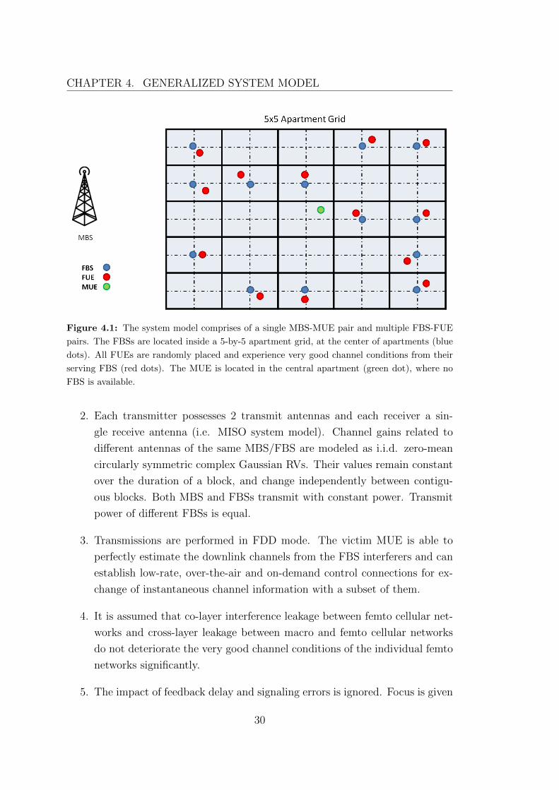
Figure 4.1: The system model comprises of a single MBS-MUE pair and multiple FBS-FUE
pairs. The FBSs are located inside a 5-by-5 apartment grid, at the center of apartments (blue
dots). All FUEs are randomly placed and experience very good channel conditions from their
serving FBS (red dots). The MUE is located in the central apartment (green dot), where no
FBS is available.
2. Each transmitter possesses 2 transmit antennas and each receiver a sin-
gle receive antenna (i.e. MISO system model). Channel gains related to
different antennas of the same MBS/FBS are modeled as i.i.d. zero-mean
circularly symmetric complex Gaussian RVs. Their values remain constant
over the duration of a block, and change independently between contigu-
ous blocks. Both MBS and FBSs transmit with constant power. Transmit
power of different FBSs is equal.
3. Transmissions are performed in FDD mode. The victim MUE is able to
perfectly estimate the downlink channels from the FBS interferers and can
establish low-rate, over-the-air and on-demand control connections for ex-
change of instantaneous channel information with a subset of them.
4. It is assumed that co-layer interference leakage between femto cellular net-
works and cross-layer leakage between macro and femto cellular networks
do not deteriorate the very good channel conditions of the individual femto
networks significantly.
5. The impact of feedback delay and signaling errors is ignored. Focus is given
30
4.2. MEAN AND INSTANTANEOUS SINR AT THE MUE
on the quantization aspect of the feedback channel.
We remark that extension of the analysis to support multiple MUEs is straight-
forward. In the case of single carrier HSDPA, different MUEs can be scheduled
in time in the shared channel, so that the altruistic behavior of the FBSs can
change accordingly between transmission time intervals (TTIs) to fit the needs of
each MUE. In the case of LTE and LTE-Advanced, hard frequency reuse can be
applied, and MUEs can be scheduled to receive in non-overlapping parts of the
spectrum, since OFDMA is used as air interface.
4.2 Mean and Instantaneous SINR at the MUE
Let S denote the set comprising of all FBSs interferers from the perspective of
the MUE. Consider the ordered set SA ⊆ S, containing those FBSs that apply
altruistic TBF to mitigate instantaneous interference at the MUE. The ranking
is performed from strongest to weakest interferer, taking into account only their
large scale fading statistics. Order is important, since our aim is to mitigate the
fast fading term of the first k strongest interferers, to provide the highest possible
performance gains. The set SE ⊆ S, which is the complement of SA, contains the
remaining FBSs that perform egoistic TBF to favor their own FUEs. The mean
received power of all egoistic FBSs with indices i ∈ SE is grouped together with
thermal noise power and treated as background interference. Therefore, order is
not important for SE.
The MBS transmits with constant transmit power Pm and all FBSs with
constant transmit power Pf . The distance dependent path loss between MBS
and MUE is denoted as Lm, while Lfi (∀i ∈ S) denotes the distance dependent
attenuation between altruistic FBSi and MUE. Thermal noise power is denoted
as Pn. The mean received SINR at the MUE can then be represented as
SINRmue =PmLm
Pn +∑i∈SE
PfLfi
+∑i∈SA
PfLfi
=PmLm
PI +∑i∈SA
PfLfi
=Pm
PI Lm
1 +∑i∈SA
PfPI Lfi
=γm
1 +∑i∈SA
γfi. (4.1)
where γm and γfi denote the mean received SINR at the MUE, from the MBS and
each FBSi respectively, when signals from egoistic users and thermal noise are
31
CHAPTER 4. GENERALIZED SYSTEM MODEL
forming the interference PI . Due to the definition of SA, the term γf1 represents
the strongest interferer.
For the modeling of the instantaneous SINR at the MUE, we consider the fast
fading component in the egoistic MBS and the altruistic FBSs. Then, the channel
between MBS and MUE is hm = [hm,1 hm,2], and the egoistic beamforming vector
applied is given by (2.1). Similarly, the channel between altruistic FBSi and MUE
is hfi = [hfi,1 hfi,2] and the beamforming vector applied by FBSi is given by (3.2).
The instantaneous SINR at the MUE is, then, given by
SINRmue =γm|hm · wm|2
1 +∑
i∈SA
γfi |hfi · wfi |2. (4.2)
4.3 System Parameters
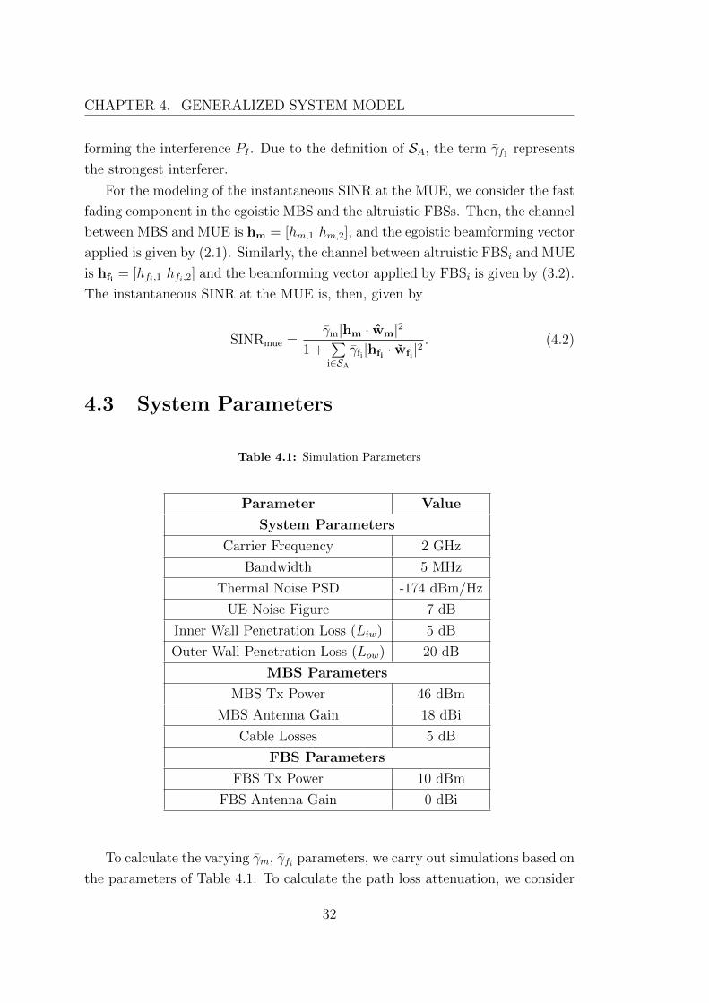
Table 4.1: Simulation Parameters
Parameter Value
System Parameters
Carrier Frequency 2 GHz
Bandwidth 5 MHz
Thermal Noise PSD -174 dBm/Hz
UE Noise Figure 7 dB
Inner Wall Penetration Loss (Liw) 5 dB
Outer Wall Penetration Loss (Low) 20 dB
MBS Parameters
MBS Tx Power 46 dBm
MBS Antenna Gain 18 dBi
Cable Losses 5 dB
FBS Parameters
FBS Tx Power 10 dBm
FBS Antenna Gain 0 dBi
To calculate the varying γm, γfi parameters, we carry out simulations based on
the parameters of Table 4.1. To calculate the path loss attenuation, we consider
32
4.4. PROBABILISTIC MODELING OF INSTANTANEOUS RECEIVEDSINR
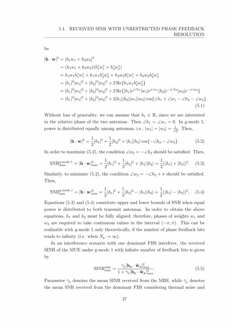
the path loss models presented in [69]. For indoor-initiated transmissions (i.e.
FBS to FUE and FBS to MUE) the path loss model is given by:
PLin(dB) = 38.46 + 20log10R + 0.7d2D,in + 18.3n((n+2)(n+1)−0.46) + q · Liw,
where R is the distance in meters between transmitter and receiver, d2D,in is the
part of this distance which is indoors, n is the number of floors that separate
transmitter and receiver, Liw is the penetration loss of inner walls and q is the
number of penetrated indoor walls that the signal must pass through. We will
study single floor cases, therefore n = 0. Also, all UEs will reside indoors, there-
fore R = d2D,in. For outdoor-initiated transmissions (i.e., MBS to FUEs and
MBS to MUE), the path loss model is given by
PLout(dB) = 15.3 + 37.6log10R + Low + q · Liw,
where the term Low refers to outer wall penetration loss.
4.4 Probabilistic Modeling of Instantaneous Re-
ceived SINR
The received instantaneous SINR of the MUE can be represented as an RV which
is a function of multiple RVs, i.e.
Z =X
1 +∑i∈SA
Yi, (4.3)
where X = γm|hm · wm|2 and Yi = γfi |hfi · wfi |2.
In following chapters, we will present analytical expressions for the cumula-
tive distribution function (CDF) of Z, denoted as FZ(z). Another illustration of
the downlink performance of the MUE is the outage probability of its spectral
efficiency (or rate distribution), which is directly obtained using FZ(z). It is well
known that downlink rate is a function of the received SINR, and specifically
R = log2(1 +Z). The CDF FR(r) of R can be given in terms of FZ(z) as follows:
FR(r) = FZ(2r − 1). (4.4)
33

CHAPTER 4. GENERALIZED SYSTEM MODEL
34
Chapter 5
Perfect Phase Altruistic
Beamforming
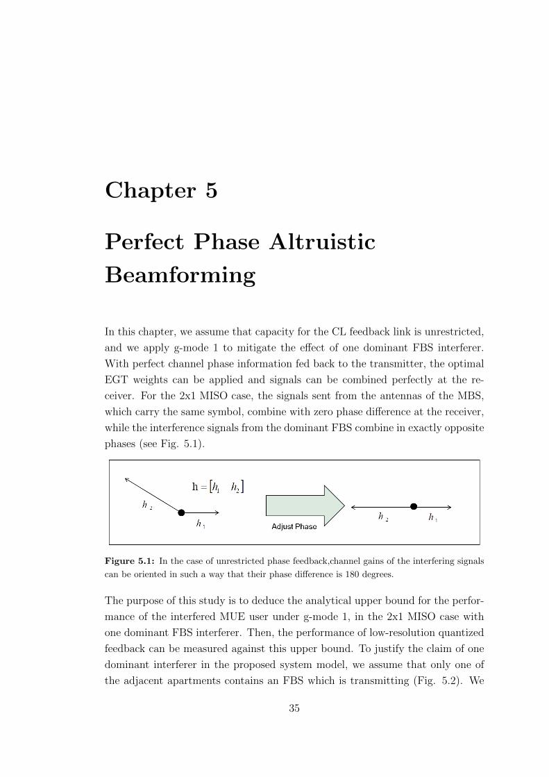
In this chapter, we assume that capacity for the CL feedback link is unrestricted,
and we apply g-mode 1 to mitigate the effect of one dominant FBS interferer.
With perfect channel phase information fed back to the transmitter, the optimal
EGT weights can be applied and signals can be combined perfectly at the re-
ceiver. For the 2x1 MISO case, the signals sent from the antennas of the MBS,
which carry the same symbol, combine with zero phase difference at the receiver,
while the interference signals from the dominant FBS combine in exactly opposite
phases (see Fig. 5.1).
Figure 5.1: In the case of unrestricted phase feedback,channel gains of the interfering signals
can be oriented in such a way that their phase difference is 180 degrees.
The purpose of this study is to deduce the analytical upper bound for the perfor-
mance of the interfered MUE user under g-mode 1, in the 2x1 MISO case with
one dominant FBS interferer. Then, the performance of low-resolution quantized
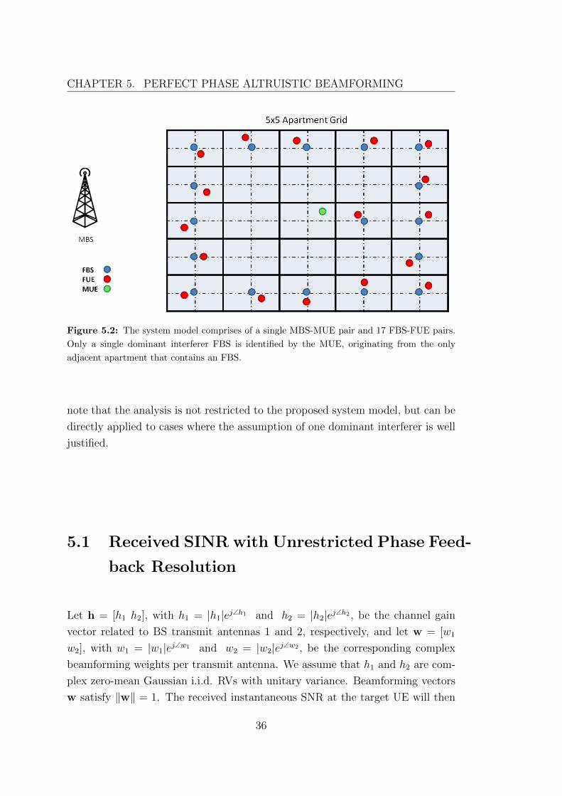
feedback can be measured against this upper bound. To justify the claim of one
dominant interferer in the proposed system model, we assume that only one of
the adjacent apartments contains an FBS which is transmitting (Fig. 5.2). We
35
CHAPTER 5. PERFECT PHASE ALTRUISTIC BEAMFORMING
Figure 5.2: The system model comprises of a single MBS-MUE pair and 17 FBS-FUE pairs.
Only a single dominant interferer FBS is identified by the MUE, originating from the only
adjacent apartment that contains an FBS.
note that the analysis is not restricted to the proposed system model, but can be
directly applied to cases where the assumption of one dominant interferer is well
justified.
5.1 Received SINR with Unrestricted Phase Feed-
back Resolution
Let h = [h1 h2], with h1 = |h1|ej∠h1 and h2 = |h2|ej∠h2 , be the channel gain
vector related to BS transmit antennas 1 and 2, respectively, and let w = [w1
w2], with w1 = |w1|ej∠w1 and w2 = |w2|ej∠w2 , be the corresponding complex
beamforming weights per transmit antenna. We assume that h1 and h2 are com-
plex zero-mean Gaussian i.i.d. RVs with unitary variance. Beamforming vectors
w satisfy ‖w‖ = 1. The received instantaneous SNR at the target UE will then
36
5.1. RECEIVED SINR WITH UNRESTRICTED PHASE FEEDBACKRESOLUTION
be
|h ·w|2 = |h1w1 + h2w2|2
= (h1w1 + h2w2)(h∗1w∗1 + h∗2w
∗2)
= h1w1h∗1w∗1 + h1w1h
∗2w∗2 + h2w2h
∗1w∗1 + h2w2h
∗2w∗2
= |h1|2|w1|2 + |h2|2|w2|2 + 2 Re{h1w1h∗2w∗2}
= |h1|2|w1|2 + |h2|2|w2|2 + 2 Re{|h1|ej∠h1|w1|ej∠w1|h2|e−j∠h2|w2|e−j∠w2}= |h1|2|w1|2 + |h2|2|w2|2 + 2|h1||h2||w1||w2| cos{∠h1 + ∠w1 − ∠h2 − ∠w2}.
(5.1)
Without loss of generality, we can assume that h1 ∈ R, since we are interested
in the relative phase of the two antennas. Then ∠h1 = ∠w1 = 0. In g-mode 1,
power is distributed equally among antennas, i.e., |w1| = |w2| = 1√2. Then,
|h ·w|2 =1
2|h1|2 +
1
2|h2|2 + |h1||h2| cos{−∠h2 − ∠w2}. (5.2)
In order to maximize (5.2), the condition ∠w2 = −∠h2 should be satisfied. Then,
SNRg-mode 1max = |h ·w|2max =
1
2|h1|2 +
1
2|h2|2 + |h1||h2| =
1
2(|h1|+ |h2|)2. (5.3)
Similarly, to minimize (5.2), the condition ∠w2 = −∠h2 + π should be satisfied.
Then,
SNRg-mode 1min = |h ·w|2min =
1
2|h1|2 +
1
2|h2|2 − |h1||h2| =
1
2(|h1| − |h2|)2. (5.4)
Equations (5.3) and (5.4) constitute upper and lower bounds of SNR when equal
power is distributed to both transmit antennas. In order to obtain the above
equations, h1 and h2 must be fully aligned; therefore, phases of weights w1 and
w2 are required to take continuous values in the interval (−π, π). This can be
realizable with g-mode 1 only theoretically, if the number of phase feedback bits
tends to infinity (i.e. when Np →∞).
In an interference scenario with one dominant FBS interferer, the received
SINR of the MUE under g-mode 1 with infinite number of feedback bits is given
by
SINRmaxmue =
γx|hx · wx|2max1 + γy|hy · wy|2min
. (5.5)
Parameter γx denotes the mean SINR received from the MBS, while γy denotes
the mean SNR received from the dominant FBS considering thermal noise and
37
CHAPTER 5. PERFECT PHASE ALTRUISTIC BEAMFORMING
signals from egoistic interferers as background interference. Vector hx = [hx1 hx2]
expresses the channel between MBS and MUE, while hy = [hy1 hy2] corresponds
to the channel between dominant FBS and MUE. Vector wx = [wx1 wx2]T is the
beamforming vector applied by the MBS to maximize the wanted SNR at the
MUE, while wy = [wy1 wy2]T is the beamforming vector applied by the dominant
FBS to minimize interference at the MUE.
In order to measure the performance of the received SINR, we will derive the
CDF of the RV
Z =X
1 + Y, (5.6)
with X = γx|hx · wx|2max and Y = γy|hy · wy|2min positive independent RVs.
5.2 Probability Distribution for Desired Signal
In this section, we present the probability density function (PDF) and CDF of
X = γx|hx · wx|2max =γx
2(|hx1|+ |hx2|)2, (5.7)
which is the squared sum of two independent Rayleigh RVs (see (A.2) − (A.4)
in Appendix A), scaled by a constant factor. Derivation of the PDF of X was
performed using the procedure found in [70] for determining the PDF of an RV
which is a function of multiple RVs. We apply this procedure step-by-step in
Appendix A (see (A.5)− (A.12)).
We find that the PDF of X is given by
fX(x) =e−
xγx
2√xγx
[−√π erf
(√ x
γx
)+ 2
√x
γxe−
xγx +
2x√π
γxerf(√ x
γx
)], (5.8)
where erf(x) = 2√π
∫ x0e−t
2dt denotes the error function.
The CDF is given by integration of (5.8):
FX(x) = −√π
√x
γxe−
xγx erf
(√x
γx
)− e−
2xγx + 1. (5.9)
38
5.3. PROBABILITY DISTRIBUTION FOR INTERFERING SIGNAL
5.3 Probability Distribution for Interfering Sig-
nal
Following the same procedure as for X, we present the PDF of
Y = γy|hy · wy|2min =γy
2(|hy1| − |hy2|)2, (5.10)
which is the squared difference of two Rayleigh variables, scaled by a constant
factor. The PDF is given by
fY (y) =e− yγy
2√yγy
[√πerfc
(√y
γy
)+ 2
√y
γye− yγy − 2y
√π
γyerfc
(√y
γy
)], (5.11)
where erfc(y) = 1− erf(y) denotes the complementary error function.
5.4 Cumulative Distribution Function of SINR
In the previous sections, we presented the exact distributions of X and Y. The
CDF of Z = X1+Y
(i.e. the CDF of the RV representing the received SINR at the
MUE) can be calculated from the following integral:
FZ(z) =
∫ ∞1
FX(zt)fY (t− 1)dt, (5.12)
where FX(x) is the CDF of X and fY (y) is the PDF of Y. Specifically,
FX(zt) =−√π
√zt
γxe−
ztγx erf
(√zt
γx
)− e−
2ztγx + 1, (5.13)
fY (t− 1) =e− t−1γy
2√γy(t− 1)
[√π −√πerf
(√t− 1
γy
)+ 2
√t− 1
γye− t−1γy −
2(t− 1)√π
γy+
2(t− 1)√π
γyerf
(√t− 1
γy
)]. (5.14)
Equation (5.12) includes the product of (5.13) and (5.14), which results to a sum
of fifteen different terms. Thus, fifteen integrals need to be calculated and added
for derivation of FZ(z). The exact integrals are presented in Appendix B (see
(B.1)− (B.15)), along with their respective solutions (see (B.17)− (B.31)), which
39
CHAPTER 5. PERFECT PHASE ALTRUISTIC BEAMFORMING
have been derived after tedious calculations. The final formula for FZ(z) is the
sum of all computed integrals:
FZ(z) = 1− A1(z) +√πe−(azbz
2+ 1γy
)(A2(z)− A3(z))− 2e−2bzA4(z)+
2e−(azbz
2+ 1γy
)(A5(z)− A6(z)), (5.15)
where
az = 1 +γxzγy
, bz =z
γx, cz =
γxzγy
, ki =(−1)i
i!(2i+ 1),
A1(z) =2e−2bztan−1
(√1 + 2
cz
)cz(1 + 2
cz)
32
+e−2bz
(1 + 2cz
),
A2(z) =∞∑n=0
kn2Γ
(3
2
)a−n+ 7
22
z bn+ 3
22
z c32z Wn+ 1
22
,−n− 5
22
(azbz
),
A3(z) =∞∑n=0
knΓ
(1
2
)a−n+ 5
22
z bn+ 1
22
z c12z Wn+ 3
22
,−n− 3
22
(azbz
),
A4(z) =∞∑n=0
n+1∑m=0
kn (n+ 1)! bmz czm! (1 + 2cz)n−m+2
,
A5(z) =∞∑n=0
∞∑m=0
knkmΓ(m+ 1)a−m+n+3
2z b
m+n+12
z cm+1z Wn−m+1
2,−n−m−2
2
(azbz
),
A6(z) =∞∑n=0
∞∑m=0
knkm2Γ(m+ 2)a−m+n+4
2z b
m+n+22
z cm+2z Wn−m
2,−n−m−3
2
(azbz
).
The results contain the Whittaker function Wλ,µ(x), which is a standard form
of a confluent hypergeometric function and one of the two solutions of Whittaker’s
equation [71]. It is evident that the exact outage probability formula for perfect
phase feedback involves cumbersome operations. The final formula requires com-
putations of nested infinite sums, some of which need numerous iterations to
converge accurately, especially at low SINR values. Despite its non-friendly na-
ture, the resulting theoretical formula proves useful, since it is an illustration
of the best possible performance improvement under g-mode 1 and serves as a
measure against practical low-rate applications of g-mode 1.
For the scenario presented in Fig. 5.2, there are 17 interferer FBSs, of which
the closest one is the dominant interferer. For this case, using the proposed
parameters of Table 4.1 (see Chapter 4), the total mean interference plus noise
power perceived by the MUE is -64.08 dBm. The MBS is placed at 117.13 meters
40
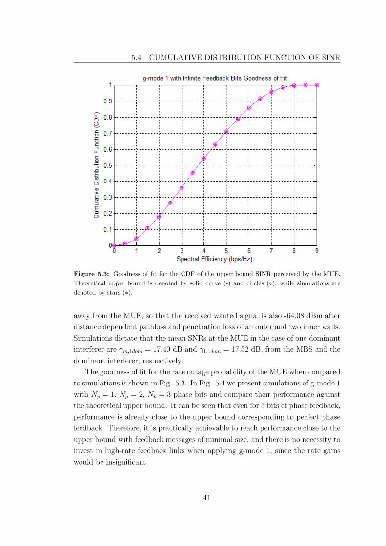
5.4. CUMULATIVE DISTRIBUTION FUNCTION OF SINR
Figure 5.3: Goodness of fit for the CDF of the upper bound SINR perceived by the MUE.
Theoretical upper bound is denoted by solid curve (-) and circles (◦), while simulations are
denoted by stars (∗).
away from the MUE, so that the received wanted signal is also -64.08 dBm after
distance dependent pathloss and penetration loss of an outer and two inner walls.
Simulations dictate that the mean SNRs at the MUE in the case of one dominant
interferer are γm,1dom = 17.40 dB and γ1,1dom = 17.32 dB, from the MBS and the
dominant interferer, respectively.
The goodness of fit for the rate outage probability of the MUE when compared
to simulations is shown in Fig. 5.3. In Fig. 5.4 we present simulations of g-mode 1
with Np = 1, Np = 2, Np = 3 phase bits and compare their performance against
the theoretical upper bound. It can be seen that even for 3 bits of phase feedback,
performance is already close to the upper bound corresponding to perfect phase
feedback. Therefore, it is practically achievable to reach performance close to the
upper bound with feedback messages of minimal size, and there is no necessity to
invest in high-rate feedback links when applying g-mode 1, since the rate gains
would be insignificant.
41
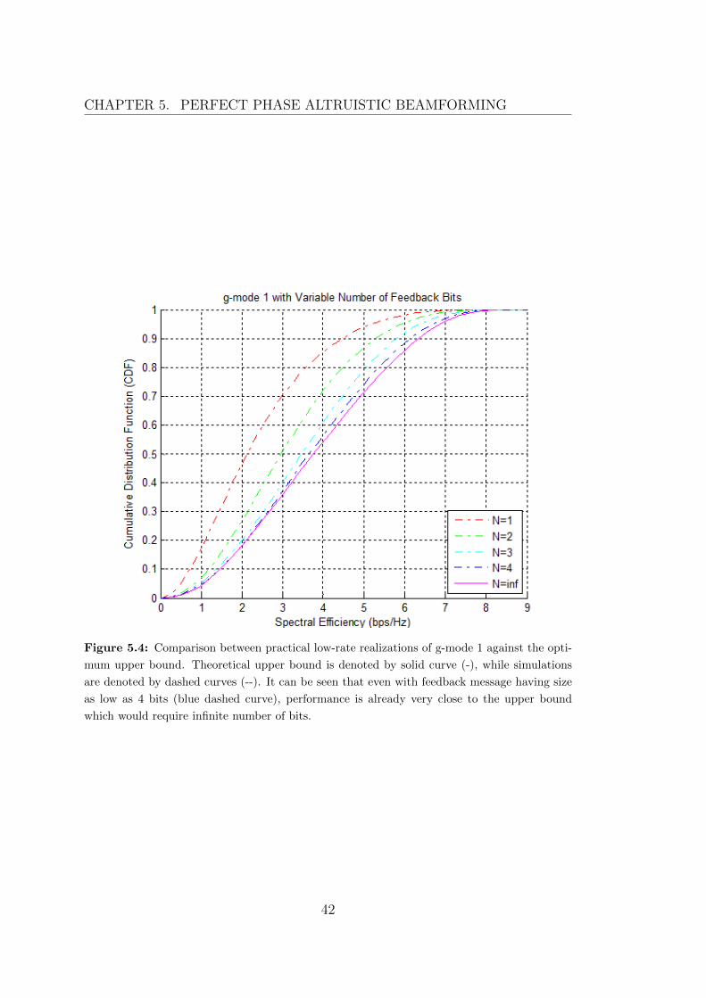
CHAPTER 5. PERFECT PHASE ALTRUISTIC BEAMFORMING
Figure 5.4: Comparison between practical low-rate realizations of g-mode 1 against the opti-
mum upper bound. Theoretical upper bound is denoted by solid curve (-), while simulations
are denoted by dashed curves (--). It can be seen that even with feedback message having size
as low as 4 bits (blue dashed curve), performance is already very close to the upper bound
which would require infinite number of bits.
42
Chapter 6
Altruistic Beamforming in
Multiple Interference Sources
In this section we investigate the SINR and rate outage probability of the MUE
as a function of the number of altruistic interferers. We consider that 24 FBSs are
transmitting simultaneously in all apartments except the central one, in which the
MUE operates (Fig. 6.1). Initially, all FBSs behave egoistically by applying TSC,
g-mode 1 or g-mode 2. One-by-one, the interferers apply altruistic TBF, starting
from the strongest interferer and gradually reaching the weakest. As shown in
section 4.4, the SINR of the MUE in the presence of multiple altruistic interferer
FBSs can be modeled as Z = X1+
∑i∈SA
Yi, where SA denotes the ordered set of altru-
istic FBSs according to received power at the MUE, X = γm|hm · wm|2 represents
the desired MBS signal, and Yi = γfi|hfi · wfi |2 represents the interference signal
from altruistic FBS i.
6.1 Chi-squared Approximations for Desired and
Interference Signals
Since exact distributions of the individual RVs (i.e. X and Yi) are generally
difficult to find, we will use those χ2 approximations presented in [72]. Thus, X
can be approximated as a χ2 RV with 4 degrees of freedom, while each interferer
43
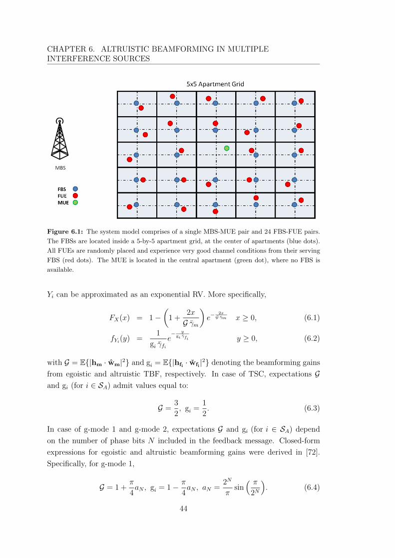
CHAPTER 6. ALTRUISTIC BEAMFORMING IN MULTIPLEINTERFERENCE SOURCES
Figure 6.1: The system model comprises of a single MBS-MUE pair and 24 FBS-FUE pairs.
The FBSs are located inside a 5-by-5 apartment grid, at the center of apartments (blue dots).
All FUEs are randomly placed and experience very good channel conditions from their serving
FBS (red dots). The MUE is located in the central apartment (green dot), where no FBS is
available.
Yi can be approximated as an exponential RV. More specifically,
FX(x) = 1−(
1 +2x
G γm
)e−
2xG γm x ≥ 0, (6.1)
fYi(y) =1
gi γfie− y
gi γfi y ≥ 0, (6.2)
with G = E{|hm · wm|2} and gi = E{|hfi · wfi|2} denoting the beamforming gains
from egoistic and altruistic TBF, respectively. In case of TSC, expectations Gand gi (for i ∈ SA) admit values equal to:
G =3
2, gi =
1
2. (6.3)
In case of g-mode 1 and g-mode 2, expectations G and gi (for i ∈ SA) depend
on the number of phase bits N included in the feedback message. Closed-form
expressions for egoistic and altruistic beamforming gains were derived in [72].
Specifically, for g-mode 1,
G = 1 +π
4aN , gi = 1− π
4aN , aN =
2N
πsin( π
2N
). (6.4)
44
6.2. EGOISTIC TBF IN ALL FBS INTERFERERS
Similarly, for g-mode 2,
G = 1 +π
4
√4
π2+ a2
N , gi = 1− π
4
√4
π2+ a2
N . (6.5)
6.2 Egoistic TBF in all FBS Interferers
For the case of |SA| = 0, where all FBS interferers apply egoistic beamforming,
the received SINR at the MUE follows a χ2 distribution with signals from all
egoistic interferers considered as background noise. Then, the outage probability
for the received SINR at the MUE is given by:
FZ
(0)mue
(z) = 1−(
1 +2z
Gγm
)e−
2zGγm z ≥ 0, (6.6)
where Z(0)mue denotes the SINR at the MUE with 0 dominant altruistic interferers,
and γm ≡ γm,|SA|=0.
6.3 Altruistic TBF only in Dominant FBS In-
terferer
For the case of |SA| = 1, where only one dominant FBS altruistic interferer is
considered, closed-form expressions for the SINR distribution of the victim MUE
have been presented in [73]. That work focused on co-layer interference, but
results directly apply to cross-layer interference scenarios, where the assumption
of a single dominant interferer is justified. The SINR outage probability for the
MUE user in case of a single dominant interferer is then given by
FZ
(1)mue
(z) = 1− e−2zG γm
[ 2z G γmg1 γf1
( G γmg1 γf1
+ 2z)2+
(1 + 2zG γm ) G γm
g1 γf1G γmg1 γf1
+ 2z
]z ≥ 0, (6.7)
where γm ≡ γm,|SA|=1 , γf1 ≡ γf1,|SA|=1.
6.4 Altruistic TBF in Multiple Dominant FBS
Interferers
In this section we assume that at least two FBS interferers apply altruistic TBF.
More specifically, we investigate two cases, in which:
45
CHAPTER 6. ALTRUISTIC BEAMFORMING IN MULTIPLEINTERFERENCE SOURCES
1. the mean received interference powers from different FBSs are different,
2. the mean received interference powers are equal. The former corresponds
to most practical real-life scenarios, while the latter represents a specific
case study with primarily theoretical value.
6.4.1 Multiple Interferers with Different Mean Received
Powers at the MUE
For cases with |SA| = `, with ` ≥ 2, we first derive the PDF of the sum∑
i∈SA Yi
of exponential RVs present in the denominator of (4.3). This requires repeated
usage of convolution, between the distributions of the interferers. For |SA| = 2,
we find that
fY (y) =
ye− y
g1 γf1
g21 γ
2f1
, if g1 γf1 = g2 γf2 ,
e− y
g2 γf2 −e− y
g1 γf1
g2 γf2−g1 γf1otherwise,
(6.8)
with y ≥ 0, γm ≡ γm,|SA|=2 , γfi ≡ γfi,|SA|=2 for i=1,2.
For the derivation of the generalized PDF, we assume that mean received pow-
ers from different transmitters differ at least slightly (i.e. gi γfi 6= gj γfj , ∀i 6= j).
This assumption, which applies to most practical scenarios, allows us to focus
on one branch of the convolution, at each stage. Then, successive convolutions
yield a pattern in the PDF derivation, which is given by the following closed-form
formula for |SA| ≥ 2:
fY (y) =
[∏i∈SA
1
gi γfi
] ∑j∈SA
e− y
gj γfj∏k 6=jk∈SA
(1
gk γfk− 1
gj γfj
) y ≥ 0. (6.9)
For details on the derivation of the above formula, see [74]. The CDF of Z can
then be calculated by substituting (6.1) and (6.9) into the following formula [75]:
FZ(z) =
∫ ∞1
FX(zt)fY (t− 1)dt. (6.10)
46
6.4. ALTRUISTIC TBF IN MULTIPLE DOMINANT FBS INTERFERERS
After manipulations, the CDF of Z for |SA| = `, with ` ≥ 2 is found to be
FZ
(`)mue
(z) =
[∏i∈SA
1
gi γfi
]×
∑j∈SA
gj γfj − e− 2zG γm
(1+G γm
2z
1+ G γm2zgj γfj
+G γm
2z
(1+ G γm2zgj γfj
)2
)∏k 6=jk∈SA
(1
gk γfk− 1
gj γfj
) z ≥ 0, (6.11)
where γm ≡ γm,|SA|=` , γfi ≡ γfi,|SA|=` for i = 1, 2, ..., `.
For illustrating the results, we assume that the MBS applies egoistic g-mode 1
with length of feedback message equal to 2 bits. Figures 6.2-6.6 illustrate the out-
age capacity distribution for the MUE, when a variable number of FBS interferers
apply altruistic TBF using TSC, g-mode 1 with 2 and 3 phase feedback bits, and
g-mode 2 with a total of 3 and 4 feedback bits (i.e. 1 bit for amplitude and the
rest for phase). In general, it can be observed that theoretical and simulation
results match very well. Slight deviations, that do not affect results significantly,
can be seen in the cases of g-mode 1 with 3 bits and g-mode 2 with 4 bits, which
result from the nature of the approximations used. Nevertheless, accurate results
are guaranteed for up to the 50th-percentile value.
For all modes, as the number of altruistic interferers increases, performance
gains can be observed until saturation is reached at the upper bound. The perfor-
mance difference between the purely egoistic (red curve) and the purely altruistic
case (black curve) is smallest in the case of TSC; thus, only few interferers need
to be considered but the improvements in outage capacity are not dramatic. The
best performance achieved by TSC for the 50th-percentile outage capacity is ap-
proximately equal to 2 bps/Hz, which denotes an almost 67 % improvement over
the egoistic case of 1.2 bps/Hz. Usage of g-mode 1 with 2 bits provides better
results than TSC and can increase the 50th-percentile rate of the MUE to a value
of about 2.8 bps/Hz with the usage of one more feedback bit. By adding one
more bit (i.e. total of 3 bits), g-mode 1 continues to improve performance (i.e.
50th-percentile reaches 3 bps/Hz) but the improvement is less noticeable. It is
clear that g-mode 2 provides the best potential for MUE performance gains, with
a possible 4.2 bps/Hz value for the 50th-percentile outage capacity, corresponding
to an improvement of around 250% compared to the egoistic case.
47
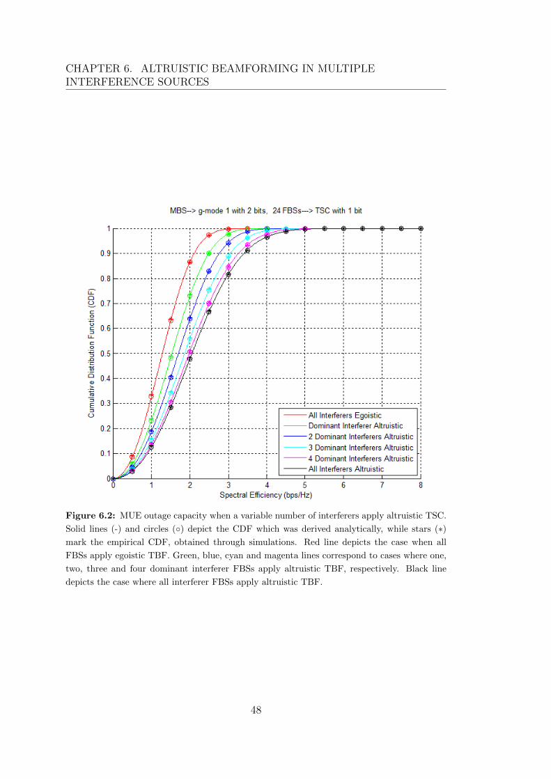
CHAPTER 6. ALTRUISTIC BEAMFORMING IN MULTIPLEINTERFERENCE SOURCES
Figure 6.2: MUE outage capacity when a variable number of interferers apply altruistic TSC.
Solid lines (-) and circles (◦) depict the CDF which was derived analytically, while stars (∗)mark the empirical CDF, obtained through simulations. Red line depicts the case when all
FBSs apply egoistic TBF. Green, blue, cyan and magenta lines correspond to cases where one,
two, three and four dominant interferer FBSs apply altruistic TBF, respectively. Black line
depicts the case where all interferer FBSs apply altruistic TBF.
48
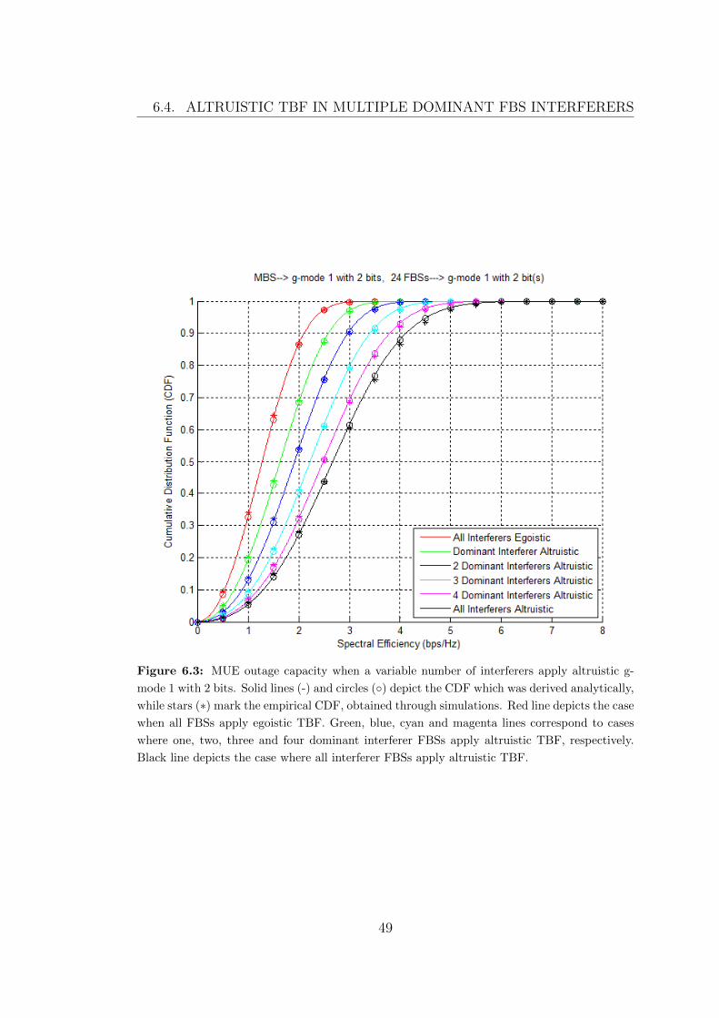
6.4. ALTRUISTIC TBF IN MULTIPLE DOMINANT FBS INTERFERERS
Figure 6.3: MUE outage capacity when a variable number of interferers apply altruistic g-
mode 1 with 2 bits. Solid lines (-) and circles (◦) depict the CDF which was derived analytically,
while stars (∗) mark the empirical CDF, obtained through simulations. Red line depicts the case
when all FBSs apply egoistic TBF. Green, blue, cyan and magenta lines correspond to cases
where one, two, three and four dominant interferer FBSs apply altruistic TBF, respectively.
Black line depicts the case where all interferer FBSs apply altruistic TBF.
49
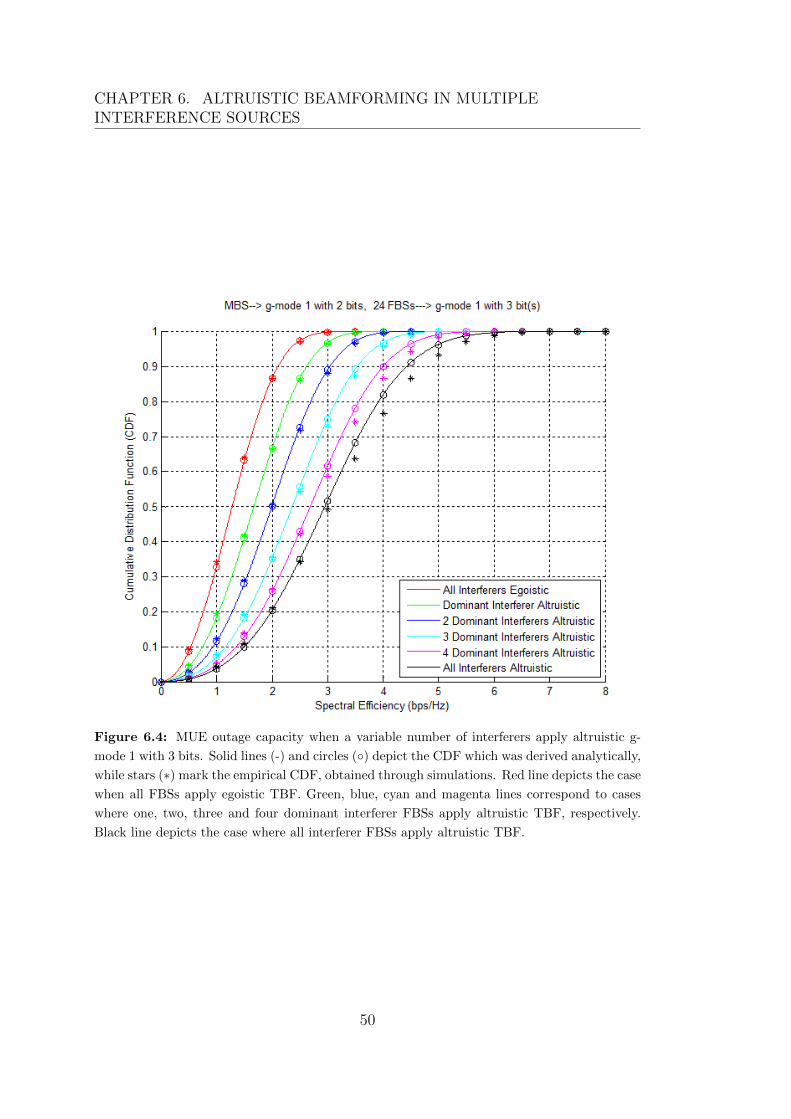
CHAPTER 6. ALTRUISTIC BEAMFORMING IN MULTIPLEINTERFERENCE SOURCES
Figure 6.4: MUE outage capacity when a variable number of interferers apply altruistic g-
mode 1 with 3 bits. Solid lines (-) and circles (◦) depict the CDF which was derived analytically,
while stars (∗) mark the empirical CDF, obtained through simulations. Red line depicts the case
when all FBSs apply egoistic TBF. Green, blue, cyan and magenta lines correspond to cases
where one, two, three and four dominant interferer FBSs apply altruistic TBF, respectively.
Black line depicts the case where all interferer FBSs apply altruistic TBF.
50

6.4. ALTRUISTIC TBF IN MULTIPLE DOMINANT FBS INTERFERERS
Figure 6.5: MUE outage capacity when a variable number of interferers apply altruistic g-
mode 2 with 3 bits (i.e. 2 phase bits and 1 amplitude bit with optimal amplitude weights).
Solid lines (-) and circles (◦) depict the CDF which was derived analytically, while stars (∗)mark the empirical CDF, obtained through simulations. Red line depicts the case when all
FBSs apply egoistic TBF. Green, blue, cyan and magenta lines correspond to cases where one,
two, three and four dominant interferer FBSs apply altruistic TBF, respectively. Black line
depicts the case where all interferer FBSs apply altruistic TBF.
51
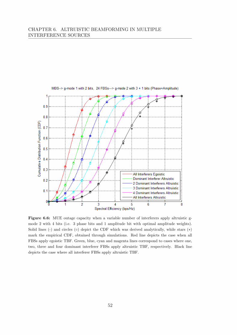
CHAPTER 6. ALTRUISTIC BEAMFORMING IN MULTIPLEINTERFERENCE SOURCES
Figure 6.6: MUE outage capacity when a variable number of interferers apply altruistic g-
mode 2 with 4 bits (i.e. 3 phase bits and 1 amplitude bit with optimal amplitude weights).
Solid lines (-) and circles (◦) depict the CDF which was derived analytically, while stars (∗)mark the empirical CDF, obtained through simulations. Red line depicts the case when all
FBSs apply egoistic TBF. Green, blue, cyan and magenta lines correspond to cases where one,
two, three and four dominant interferer FBSs apply altruistic TBF, respectively. Black line
depicts the case where all interferer FBSs apply altruistic TBF.
52
6.4. ALTRUISTIC TBF IN MULTIPLE DOMINANT FBS INTERFERERS
The 10th and 50th percentile spectral efficiency values are illustrated in figures
6.7 and 6.8 respectively. Curves for complete CSIT and complete phase CSIT
have also been included for comparison. It is evident that mitigation of more
than 12 interferers provides almost no gain for the MUE, independent of the
mode used. Thus, there is no need to sacrifice the beamforming gain of any of
the 12 weakest interferers. Most importantly, it can be observed that curves have
almost constant slope for certain groups of altruistic interferers. This observation
yields that application of altruistic TBF provides best gains when it is performed
in clusters, taking advantage of the system topology. For the specific system
presented in Fig. 6.1, it is best to consider clusters of four interferers. The
first cluster consists of the four dominant interferers and the remaining clusters
are defined in a similar way, according to their level of mean interference power
towards the MUE.
Consider the 10th-percentile outage capacity of Fig. 6.7. For the TSC case,
mitigation of the first cluster is enough for reaching the performance upper bound.
For g-mode 1, mitigation of at most two clusters is sufficient for reaching the up-
per bound. Indeed, even for infinite number of available phase feedback bits,
considering more clusters provides no gain in performance. Algorithm g-mode 2
with 4 bits is the only method of those with limited feedback that still provides
noticeable gains in the 10th-percentile outage capacity when considering a third
cluster. In general, the above observations also apply for the 50th- percentile
outage capacity (see Fig. 6.8), even though there can be observed slight improve-
ments when considering a second cluster for TSC or a third cluster for g-mode 1.
From the above observations, it is clear that the optimal number of participating
clusters depends on the mode used and the chosen resolution for the feedback
message.
53
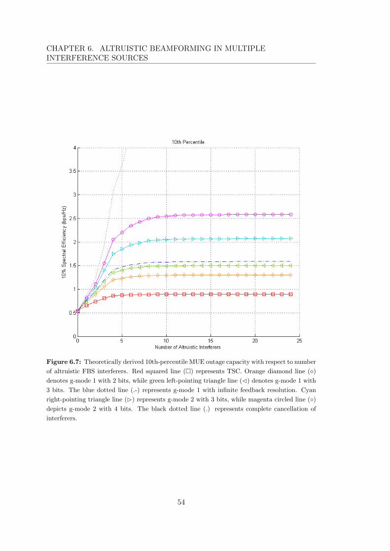
CHAPTER 6. ALTRUISTIC BEAMFORMING IN MULTIPLEINTERFERENCE SOURCES
Figure 6.7: Theoretically derived 10th-percentile MUE outage capacity with respect to number
of altruistic FBS interferers. Red squared line (�) represents TSC. Orange diamond line (�)denotes g-mode 1 with 2 bits, while green left-pointing triangle line (C) denotes g-mode 1 with
3 bits. The blue dotted line (.-) represents g-mode 1 with infinite feedback resolution. Cyan
right-pointing triangle line (B) represents g-mode 2 with 3 bits, while magenta circled line (◦)depicts g-mode 2 with 4 bits. The black dotted line (.) represents complete cancellation of
interferers.
54
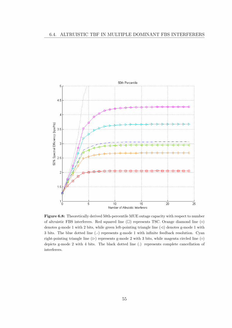
6.4. ALTRUISTIC TBF IN MULTIPLE DOMINANT FBS INTERFERERS
Figure 6.8: Theoretically derived 50th-percentile MUE outage capacity with respect to number
of altruistic FBS interferers. Red squared line (�) represents TSC. Orange diamond line (�)denotes g-mode 1 with 2 bits, while green left-pointing triangle line (C) denotes g-mode 1 with
3 bits. The blue dotted line (.-) represents g-mode 1 with infinite feedback resolution. Cyan
right-pointing triangle line (B) represents g-mode 2 with 3 bits, while magenta circled line (◦)depicts g-mode 2 with 4 bits. The black dotted line (.) represents complete cancellation of
interferers.
55
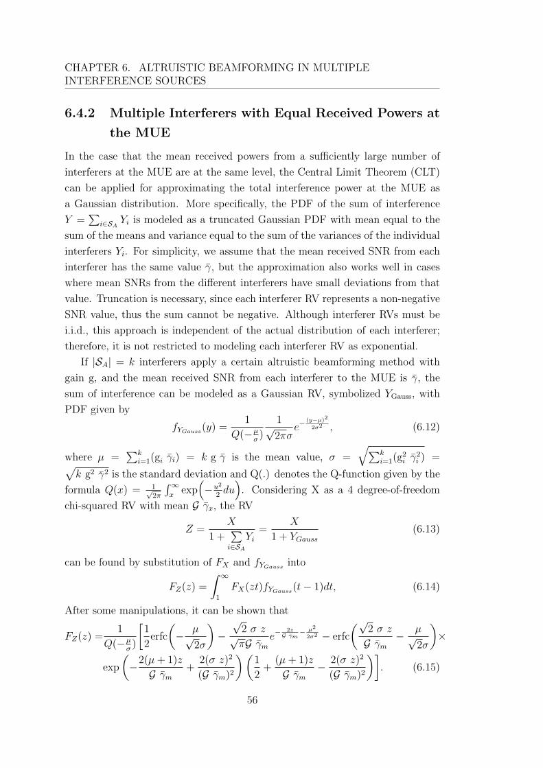
CHAPTER 6. ALTRUISTIC BEAMFORMING IN MULTIPLEINTERFERENCE SOURCES
6.4.2 Multiple Interferers with Equal Received Powers at
the MUE
In the case that the mean received powers from a sufficiently large number of
interferers at the MUE are at the same level, the Central Limit Theorem (CLT)
can be applied for approximating the total interference power at the MUE as
a Gaussian distribution. More specifically, the PDF of the sum of interference
Y =∑
i∈SA Yi is modeled as a truncated Gaussian PDF with mean equal to the
sum of the means and variance equal to the sum of the variances of the individual
interferers Yi. For simplicity, we assume that the mean received SNR from each
interferer has the same value γ, but the approximation also works well in cases
where mean SNRs from the different interferers have small deviations from that
value. Truncation is necessary, since each interferer RV represents a non-negative
SNR value, thus the sum cannot be negative. Although interferer RVs must be
i.i.d., this approach is independent of the actual distribution of each interferer;
therefore, it is not restricted to modeling each interferer RV as exponential.
If |SA| = k interferers apply a certain altruistic beamforming method with
gain g, and the mean received SNR from each interferer to the MUE is γ, the
sum of interference can be modeled as a Gaussian RV, symbolized YGauss, with
PDF given by
fYGauss(y) =1
Q(−µσ)
1√2πσ
e−(y−µ)2
2σ2 , (6.12)
where µ =∑k
i=1(gi γi) = k g γ is the mean value, σ =√∑k
i=1(g2i γ
2i ) =√
k g2 γ2 is the standard deviation and Q(.) denotes the Q-function given by the
formula Q(x) = 1√2π
∫∞x
exp(−u2
2du)
. Considering X as a 4 degree-of-freedom
chi-squared RV with mean G γx, the RV
Z =X
1 +∑i∈SA
Yi=
X
1 + YGauss(6.13)
can be found by substitution of FX and fYGauss into
FZ(z) =
∫ ∞1
FX(zt)fYGauss(t− 1)dt, (6.14)
After some manipulations, it can be shown that
FZ(z) =1
Q(−µσ)
[1
2erfc
(− µ√
2σ
)−√
2 σ z√πG γm
e−2zG γm
− µ2
2σ2 − erfc
(√2 σ z
G γm− µ√
2σ
)×
exp
(−2(µ+ 1)z
G γm+
2(σ z)2
(G γm)2
)(1
2+
(µ+ 1)z
G γm− 2(σ z)2
(G γm)2
)]. (6.15)
56
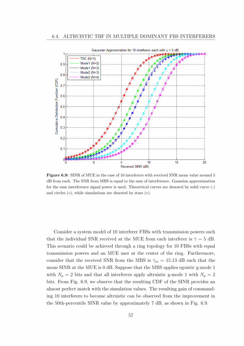
6.4. ALTRUISTIC TBF IN MULTIPLE DOMINANT FBS INTERFERERS
Figure 6.9: SINR of MUE in the case of 10 interferers with received SNR mean value around 5
dB from each. The SNR from MBS is equal to the sum of interference. Gaussian approximation
for the sum interference signal power is used. Theoretical curves are denoted by solid curve (-)
and circles (◦), while simulations are denoted by stars (∗).
Consider a system model of 10 interferer FBSs with transmission powers such
that the individual SNR received at the MUE from each interferer is γ = 5 dB.
This scenario could be achieved through a ring topology for 10 FBSs with equal
transmission powers and an MUE user at the center of the ring. Furthermore,
consider that the received SNR from the MBS is γm = 15.13 dB such that the
mean SINR at the MUE is 0 dB. Suppose that the MBS applies egoistic g-mode 1
with Np = 2 bits and that all interferers apply altruistic g-mode 1 with Np = 2
bits. From Fig. 6.9, we observe that the resulting CDF of the SINR provides an
almost perfect match with the simulation values. The resulting gain of command-
ing 10 interferers to become altruistic can be observed from the improvement in
the 50th-percentile SINR value by approximately 7 dB, as shown in Fig. 6.9.
57
CHAPTER 6. ALTRUISTIC BEAMFORMING IN MULTIPLEINTERFERENCE SOURCES
6.5 Performance Degradation at the FUE
So far, we have dealt only with the performance of the MUE. Initially, from the
perspective of an FUE served by an egoistic FBS, the SINR follows a χ2 distri-
bution with 4 degrees of freedom and mean Gf γf , where Gf is the beamforming
gain from the TBF method applied at the FBS, and γf is the mean SINR per-
ceived at the FUE. This is due to the fact that all of its perceived interferers (i.e.
the remaining FBSs and the MBS) are treated as background noise, since no co-
channel interference mitigation is performed by other BSs towards the particular
FUE (i.e. |SAf | = 0). The CDF of the SINR for the FUE, assuming that its
serving FBS is egoistic, is given by
FZ
(0)fue
(z) = 1−(
1 +2z
Gγf
)e− 2zGγf z ≥ 0, (6.16)
where Z(0)fue denotes the SINR at the FUE with 0 dominant altruistic interferers,
and γf ≡ γf,|SAf |=0 denotes the respective mean SINR at the FUE.
When the FBS shifts its behavior from egoistic to altruistic, the desired signal
X received by its associated FUE becomes exponentially distributed with mean
γf . Then, the SINR at the FUE follows an exponential distribution:
FZ
(0)fue
(z) = 1− e−zγf , z ≥ 0. (6.17)
Mean loss of performance for each FUE, when its serving FBS applies altruistic
TBF, is equal to the beamforming gain G that is not present anymore. In a high
SINR regime, this is usually equivalent to an insignificant loss in achievable data
rate.
58
Chapter 7
Extensions of Altruistic
Beamforming Methods
So far, in order to improve performance of an interfered MUE in a HetNet set-
ting, we have used the practical algorithms of TSC, g-mode 1 and g-mode 2 for
interference mitigation exactly as found in [66][73] for the two-antenna case. In
this chapter, we investigate modifications of these methods to
1. include more precise amplitude feedback, and
2. to work efficiently when transmitters possess more than two transmit an-
tennas.
As an initial study, we will concentrate in adding one more bit for amplitude
resolution in the feedback message of g-mode 2. In addition, we will present our
multi-antenna interference scheme for the case of 4 antennas, which can easily be
generalized for 2n, where n ∈ N represents the number of transmit antennas.
7.1 Increasing Amplitude Feedback Resolution
Although the feedback message of g-mode 2 contains information about the order
of channel gain amplitudes, it is clear that primary emphasis has been given on
the phase resolution. For the case of two transmit antennas, g-mode 2 dedicates
only one bit for the feedback of channel amplitude information. Therefore, the
only permitted action regarding amplitude information is feeding back to the
transmitter the index corresponding to the strongest/weakest antenna. Consider
the case where the amplitudes of the two channel gains are approximately equal.
59
CHAPTER 7. EXTENSIONS OF ALTRUISTIC BEAMFORMINGMETHODS
Then, the receiver must identify and send back to the transmitter the index of the
best antenna (i.e., for interference mitigation, the one with the weakest channel),
without providing information about the strength relationship between antennas.
Thus, considering optimal amplitude weights, approximately 80 % of the power
will be allocated to the slightly better antenna, and only 20 % to the weaker
antenna, although their channel conditions are similar. This example signifies
that knowledge of the relative strength between the two channel gains (i.e., soft
order information) could further improve the performance of g-mode 2.
In this section, we investigate the performance of increased amplitude feedback
resolution for altruistic beamforming, in cases where interferers are equipped
with two transmit antennas. More specifically, we consider that the feedback
message contains two bits dedicated to amplitude information and the remaining
for phase. We define a threshold value for the difference between the amplitudes
of the two channel gains. Then, different amplitude weights are applied when
the instantaneous amplitude difference of the channel gains is higher or lower
than the predefined threshold. By means of a brute force search, we identify the
optimal amplitude weights that should be applied for a given threshold. More
specifically, we vary the threshold value between the two channel gain amplitudes
from 1 to 10 dB in unitary dB steps. Then, for each threshold, brute force
search is performed to find optimal amplitude weights for cases where the channel
amplitude difference is above and below the threshold. The optimal amplitude
weights for a list of threshold values are shown in tables 7.1-7.4, together with
the respective SNR gains perceived by the victim MUE on the interference link
(i.e. the weaker the signal received, the higher the gain for the MUE), against the
case where no beamforming is used and SNR gain is 0 dB. Each amplitude weight
vector contains two amplitude weights, with the first/smallest value applied to
the strongest antenna. In all cases, the optimal threshold values for a fixed-length
feedback message are shown in bold. These are the values that will be chosen for
comparisons against traditional g-mode 2.
60
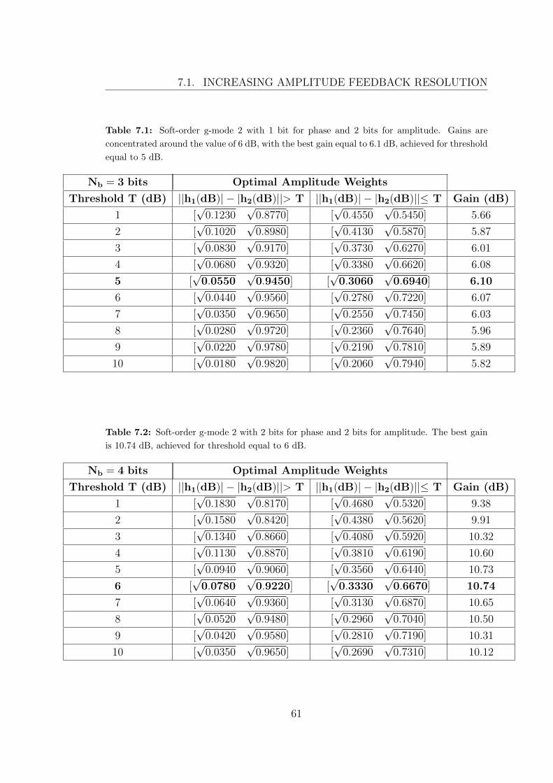
7.1. INCREASING AMPLITUDE FEEDBACK RESOLUTION
Table 7.1: Soft-order g-mode 2 with 1 bit for phase and 2 bits for amplitude. Gains are
concentrated around the value of 6 dB, with the best gain equal to 6.1 dB, achieved for threshold
equal to 5 dB.
Nb = 3 bits Optimal Amplitude Weights
Threshold T (dB) ||h1(dB)| − |h2(dB)||> T ||h1(dB)| − |h2(dB)||≤ T Gain (dB)
1 [√
0.1230√
0.8770] [√
0.4550√
0.5450] 5.66
2 [√
0.1020√
0.8980] [√
0.4130√
0.5870] 5.87
3 [√
0.0830√
0.9170] [√
0.3730√
0.6270] 6.01
4 [√
0.0680√
0.9320] [√
0.3380√
0.6620] 6.08
5 [√
0.0550√
0.9450] [√
0.3060√
0.6940] 6.10
6 [√
0.0440√
0.9560] [√
0.2780√
0.7220] 6.07
7 [√
0.0350√
0.9650] [√
0.2550√
0.7450] 6.03
8 [√
0.0280√
0.9720] [√
0.2360√
0.7640] 5.96
9 [√
0.0220√
0.9780] [√
0.2190√
0.7810] 5.89
10 [√
0.0180√
0.9820] [√
0.2060√
0.7940] 5.82
Table 7.2: Soft-order g-mode 2 with 2 bits for phase and 2 bits for amplitude. The best gain
is 10.74 dB, achieved for threshold equal to 6 dB.
Nb = 4 bits Optimal Amplitude Weights
Threshold T (dB) ||h1(dB)| − |h2(dB)||> T ||h1(dB)| − |h2(dB)||≤ T Gain (dB)
1 [√
0.1830√
0.8170] [√
0.4680√
0.5320] 9.38
2 [√
0.1580√
0.8420] [√
0.4380√
0.5620] 9.91
3 [√
0.1340√
0.8660] [√
0.4080√
0.5920] 10.32
4 [√
0.1130√
0.8870] [√
0.3810√
0.6190] 10.60
5 [√
0.0940√
0.9060] [√
0.3560√
0.6440] 10.73
6 [√
0.0780√
0.9220] [√
0.3330√
0.6670] 10.74
7 [√
0.0640√
0.9360] [√
0.3130√
0.6870] 10.65
8 [√
0.0520√
0.9480] [√
0.2960√
0.7040] 10.50
9 [√
0.0420√
0.9580] [√
0.2810√
0.7190] 10.31
10 [√
0.0350√
0.9650] [√
0.2690√
0.7310] 10.12
61
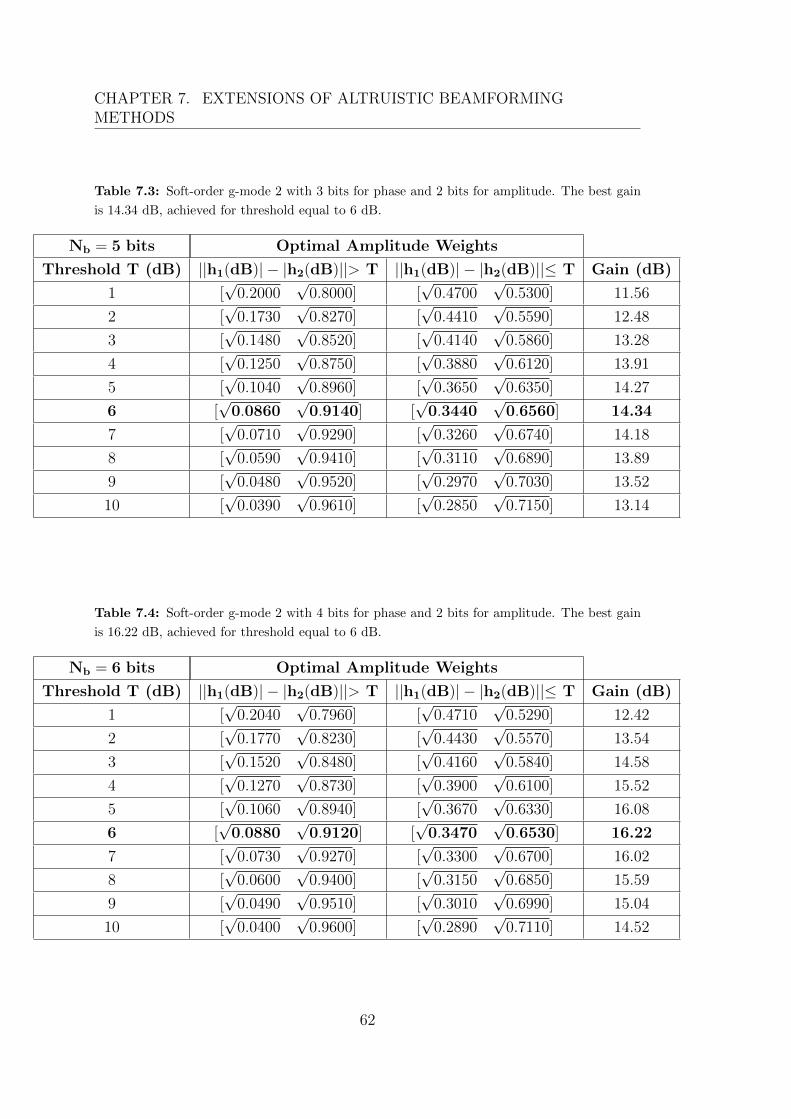
CHAPTER 7. EXTENSIONS OF ALTRUISTIC BEAMFORMINGMETHODS
Table 7.3: Soft-order g-mode 2 with 3 bits for phase and 2 bits for amplitude. The best gain
is 14.34 dB, achieved for threshold equal to 6 dB.
Nb = 5 bits Optimal Amplitude Weights
Threshold T (dB) ||h1(dB)| − |h2(dB)||> T ||h1(dB)| − |h2(dB)||≤ T Gain (dB)
1 [√
0.2000√
0.8000] [√
0.4700√
0.5300] 11.56
2 [√
0.1730√
0.8270] [√
0.4410√
0.5590] 12.48
3 [√
0.1480√
0.8520] [√
0.4140√
0.5860] 13.28
4 [√
0.1250√
0.8750] [√
0.3880√
0.6120] 13.91
5 [√
0.1040√
0.8960] [√
0.3650√
0.6350] 14.27
6 [√
0.0860√
0.9140] [√
0.3440√
0.6560] 14.34
7 [√
0.0710√
0.9290] [√
0.3260√
0.6740] 14.18
8 [√
0.0590√
0.9410] [√
0.3110√
0.6890] 13.89
9 [√
0.0480√
0.9520] [√
0.2970√
0.7030] 13.52
10 [√
0.0390√
0.9610] [√
0.2850√
0.7150] 13.14
Table 7.4: Soft-order g-mode 2 with 4 bits for phase and 2 bits for amplitude. The best gain
is 16.22 dB, achieved for threshold equal to 6 dB.
Nb = 6 bits Optimal Amplitude Weights
Threshold T (dB) ||h1(dB)| − |h2(dB)||> T ||h1(dB)| − |h2(dB)||≤ T Gain (dB)
1 [√
0.2040√
0.7960] [√
0.4710√
0.5290] 12.42
2 [√
0.1770√
0.8230] [√
0.4430√
0.5570] 13.54
3 [√
0.1520√
0.8480] [√
0.4160√
0.5840] 14.58
4 [√
0.1270√
0.8730] [√
0.3900√
0.6100] 15.52
5 [√
0.1060√
0.8940] [√
0.3670√
0.6330] 16.08
6 [√
0.0880√
0.9120] [√
0.3470√
0.6530] 16.22
7 [√
0.0730√
0.9270] [√
0.3300√
0.6700] 16.02
8 [√
0.0600√
0.9400] [√
0.3150√
0.6850] 15.59
9 [√
0.0490√
0.9510] [√
0.3010√
0.6990] 15.04
10 [√
0.0400√
0.9600] [√
0.2890√
0.7110] 14.52
62
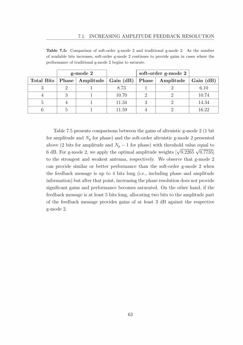
7.1. INCREASING AMPLITUDE FEEDBACK RESOLUTION
Table 7.5: Comparison of soft-order g-mode 2 and traditional g-mode 2. As the number
of available bits increases, soft-order g-mode 2 continues to provide gains in cases where the
performance of traditional g-mode 2 begins to saturate.
g-mode 2 soft-order g-mode 2
Total Bits Phase Amplitude Gain (dB) Phase Amplitude Gain (dB)
3 2 1 8.73 1 2 6.10
4 3 1 10.70 2 2 10.74
5 4 1 11.34 3 2 14.34
6 5 1 11.59 4 2 16.22
Table 7.5 presents comparisons between the gains of altruistic g-mode 2 (1 bit
for amplitude and Np for phase) and the soft-order altruistic g-mode 2 presented
above (2 bits for amplitude and Np − 1 for phase) with threshold value equal to
6 dB. For g-mode 2, we apply the optimal amplitude weights [√
0.2265√
0.7735]
to the strongest and weakest antenna, respectively. We observe that g-mode 2
can provide similar or better performance than the soft-order g-mode 2 when
the feedback message is up to 4 bits long (i.e., including phase and amplitude
information) but after that point, increasing the phase resolution does not provide
significant gains and performance becomes saturated. On the other hand, if the
feedback message is at least 5 bits long, allocating two bits to the amplitude part
of the feedback message provides gains of at least 3 dB against the respective
g-mode 2.
63
CHAPTER 7. EXTENSIONS OF ALTRUISTIC BEAMFORMINGMETHODS
7.2 Increasing the Number of Transmit Anten-
nas
In the case of egoistic TBF, the algorithms of TSC, g-mode 1 and g-mode 2 are
applicable to cases in which transmitters are equipped with more than two anten-
nas. For g-mode 1, all phase modifications are made against a reference antenna,
and, although this method is suboptimal and depends on the choice of reference
antenna, gains can be achieved. For g-mode 2, amplitudes can be chosen in such
a way that the strongest channel gains are favored. In the case of altruistic beam-
forming, though, adaptation of the algorithms is not as straightforward, except
for TSC. Clearly g-mode 1 does not work, since directing all channel gains in
phase opposition against just a single reference antenna is equivalent to a ran-
dom outcome in the received signal. The best choice would be for the interfered
MUE to test every possible beamforming vector of the predefined codebook to
find the optimal one, according to equation (3.2). The problem with this brute
force strategy is that it requires |W| beamforming vector tests, where W is the
codebook containing all the possible beamforming vectors. For g-mode 1,
|W| = 2Np(Nt−1), (7.1)
where Np is the number of phase bits in the feedback message, and Nt is the
number of transmit antennas. Therefore, when the number of antenna elements
grows from Nt to 2Nt, cardinality |W| increases rapidly by a factor of 2NpNt .
Thus, finding the optimal weight requires heavy computations and possibly high
delays, as transmitters become equipped with more and more antennas.
One option to bypass this problem is to group antenna elements in pairs.
Then, application of altruistic g-mode 1 or g-mode 2 in their initial two-antenna
form is possible, and the resulting channel gains from each pair are again grouped
until only one channel gain remains. This algorithm requires multi-stage appli-
cation of TBF, and can provide gains simply applying the original two-antenna
algorithms multiple times. With this scheme, the gains are suboptimal, but the
advantage is its more practical implementation against the brute force method
mentioned above.
We will consider the case where transmitters are equipped with Nt = 4 trans-
mit antennas. Antennas are not ranked according to their channel gain amplitude
orders, but are randomly grouped into two pairs. Then, in the first stage, the
same altruistic TBF method is applied to each pair separately. The outcome is
64
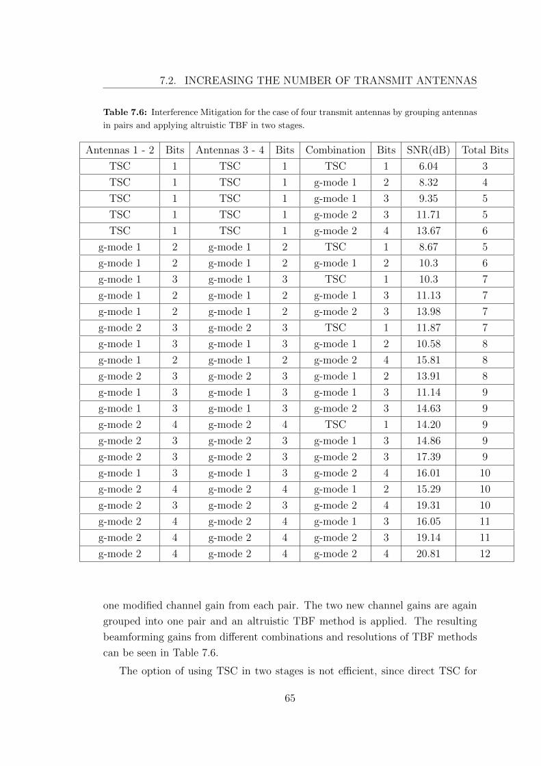
7.2. INCREASING THE NUMBER OF TRANSMIT ANTENNAS
Table 7.6: Interference Mitigation for the case of four transmit antennas by grouping antennas
in pairs and applying altruistic TBF in two stages.
Antennas 1 - 2 Bits Antennas 3 - 4 Bits Combination Bits SNR(dB) Total Bits
TSC 1 TSC 1 TSC 1 6.04 3
TSC 1 TSC 1 g-mode 1 2 8.32 4
TSC 1 TSC 1 g-mode 1 3 9.35 5
TSC 1 TSC 1 g-mode 2 3 11.71 5
TSC 1 TSC 1 g-mode 2 4 13.67 6
g-mode 1 2 g-mode 1 2 TSC 1 8.67 5
g-mode 1 2 g-mode 1 2 g-mode 1 2 10.3 6
g-mode 1 3 g-mode 1 3 TSC 1 10.3 7
g-mode 1 2 g-mode 1 2 g-mode 1 3 11.13 7
g-mode 1 2 g-mode 1 2 g-mode 2 3 13.98 7
g-mode 2 3 g-mode 2 3 TSC 1 11.87 7
g-mode 1 3 g-mode 1 3 g-mode 1 2 10.58 8
g-mode 1 2 g-mode 1 2 g-mode 2 4 15.81 8
g-mode 2 3 g-mode 2 3 g-mode 1 2 13.91 8
g-mode 1 3 g-mode 1 3 g-mode 1 3 11.14 9
g-mode 1 3 g-mode 1 3 g-mode 2 3 14.63 9
g-mode 2 4 g-mode 2 4 TSC 1 14.20 9
g-mode 2 3 g-mode 2 3 g-mode 1 3 14.86 9
g-mode 2 3 g-mode 2 3 g-mode 2 3 17.39 9
g-mode 1 3 g-mode 1 3 g-mode 2 4 16.01 10
g-mode 2 4 g-mode 2 4 g-mode 1 2 15.29 10
g-mode 2 3 g-mode 2 3 g-mode 2 4 19.31 10
g-mode 2 4 g-mode 2 4 g-mode 1 3 16.05 11
g-mode 2 4 g-mode 2 4 g-mode 2 3 19.14 11
g-mode 2 4 g-mode 2 4 g-mode 2 4 20.81 12
one modified channel gain from each pair. The two new channel gains are again
grouped into one pair and an altruistic TBF method is applied. The resulting
beamforming gains from different combinations and resolutions of TBF methods
can be seen in Table 7.6.
The option of using TSC in two stages is not efficient, since direct TSC for
65
CHAPTER 7. EXTENSIONS OF ALTRUISTIC BEAMFORMINGMETHODS
4 antennas provides the same 6 dB gain with only 2 bits. The most efficient
combinations require the presence of g-mode 2, at least in the last stage. Com-
parisons with two-antenna schemes prove the efficiency of having more antennas.
With as low as 5 feedback bits, performance of traditional two-antenna g-mode
2 with 4 bits (approximately 10.7 dB) is already surpassed (11.71 dB) and gains
continue to rise as the number of available feedback bits increases. The highest
gain is approximately 20.81 dB and requires exclusive usage of g-mode 2 with 4
bits for each pair. In total, 12 bits are required for the feedback message. It is
worth noting that a similar gain could be achieved with 9 bits (21.45 dB), if brute
force search was used to repeatedly test all 83 = 512 beamforming vectors of the
g-mode 1 codebook for four antennas. Therefore, the proposed scheme has the
advantage of not demanding time-consuming computations at the receiver side,
but the trade-off is that the feedback channel rate should be quite higher.
66
Chapter 8
Conclusions and Future Work
Cross-layer interference scenarios in two-tier heterogeneous networks could neg-
atively influence the overall network performance. The bottleneck is usually the
downlink direction, since macro base stations are typically considered as primary
infrastructure. In this thesis, we have presented results about the performance
improvements that altruistic TBF can introduce to an MUE which is heavily
interfered by a group of FBSs.
8.1 Conclusions
We have derived analytical formulas for the upper bound of the received SINR at
the MUE, in cases where a single dominant interferer applies altruistic TBF with
perfect phase resolution. Results dictate that performance close to the upper
bound can practically be achieved by using as low as 4 feedback bits, instead of
infinite.
We have investigated the case of multiple interferers, and derived the respec-
tive analytical results for the SINR improvements at the MUE. We deduce that
it is not vital to cancel every interferer, but only the cluster of closest interferers.
In practice, this number will typically be quite low, since FBSs are not installed
in every apartment and do not transmit 100 % of the time. Thus, altruistic
beamforming can provide great improvements with minimal sacrifices.
Finally, we have investigated and presented simulation results about possible
extensions of the altruistic beamforming methods. By adding one more amplitude
bit in g-mode 2, we have observed that performance can be improved significantly,
but only when the feedback message is at least 5 bits long. Similarly, we have
67
CHAPTER 8. CONCLUSIONS AND FUTURE WORK
tested an interference mitigation scheme that groups antennas in pairs and per-
forms altruistic TBF methods for each pair. This method is suboptimal, but can
provide similar gains to the two-antenna case with straightforward implementa-
tion.
8.2 Future Work
The work presented in this thesis could be extended in future studies, in the
following possible research directions:
1. Instead of including just one beamforming vector, the feedback message
from the interfered MUE towards each interferer FBS could include multiple
beamforming vectors that are sufficient for combating received interference
at the MUE (e.g. as in [67]). Then, the interferer FBS is not forced to
behave altruistic, but has the capability to choose the beamforming vector
that degrades performance for its own FUE as little as possible. The number
of beamforming vectors that are fed back determines the level of bargaining
between the performance improvement of the MUE and the performance
degradation of the respective FUE. Further analysis and application of such
a feedback scheme to various two-tier scenarios is of great interest.
2. For the two-antenna case of soft-order g-mode 2 with 2 bits of amplitude
feedback, analytical work could be carried out for the derivation of the exact
amplitude weights that minimize interference, given the optimal thresh-
old value for the amplitude difference. Furthermore, the performance of
g-mode 2 with more than 2 bits reserved for amplitude could be investi-
gated.
3. When transmitters are equipped with more than two transmit antennas,
useful approximations could be derived for efficient modeling of the prob-
ability distribution of the received SNR, when the goal is combating in-
terference by grouping the antenna elements. In addition, investigation of
new methods for direct interference mitigation without grouping of antenna
elements could be considered.
4. When transmitters are equipped with more than two transmit antennas,
useful approximations could be derived for efficient modeling of the prob-
ability distribution of the received SNR, when the goal is combating in-
68

8.2. FUTURE WORK
terference by grouping the antenna elements. In addition, investigation of
new methods for direct interference mitigation without grouping of antenna
elements could be considered.
69

CHAPTER 8. CONCLUSIONS AND FUTURE WORK
70
Bibliography
[1] Ericsson, On the Pulse of the Networking Society, White paper, Jun. 2012.
[2] Qualcomm Incorporated, LTE Advanced: Heterogeneous Networks,
White paper, Jan. 2011.
[3] H. Liang, J. I. Payne, H. S. Kim, Femto-Cells: Problem or Solution? A Net-
work Cost Analysis, in Proc. IEEE Global Telecommunications Conference,
pp. 1-6, Dec. 2011.
[4] D. Lopez-Perez, I. Guvenc, G. de la Roche, M. Kountouris, T. Q. S. Quek, J.
Zhang, Enhanced Intercell Interference Coordination Challenges in Hetero-
geneous Networks, IEEE Wireless Communications, vol. 41, no. 2, pp. 22-30,
Jun. 2011.
[5] A. Bou Saleh, S. Redana, B. Raaf, J. Hamalainen, Comparison of Relay and
Pico eNB Deployments in LTE-Advanced, in Proc. IEEE Vehicular Technol-
ogy Conference, pp. 1-5, Sep. 2009.
[6] S. Kaimaletu, R. Krishnan, S. Kalyani, N. Akhtar, B. Ramamurthi, Cogni-
tive Interference Management in Heterogeneous Femto-Macro Cell Networks,
in Proc. IEEE International Conference on Communications, pp. 1-6, Jun.
2011.
[7] Femto Forum, Femto Forum Summary Report: Interference Management in
UMTS Femtocells, White paper, Feb. 2010.
[8] D. J. Love, R. W. Heath, V. K. N. Lau, D. Gesbert, B. D. Rao, M. Andrews,
An Overview of Limited Feedback in Wireless Communication Systems, IEEE
Journal on Selected Areas in Communications, vol. 26, no. 8, pp. 1341-1365,
Oct. 2008.
71
BIBLIOGRAPHY
[9] V. Chandrasekhar, J. G. Andrews, T. Muharemovic, Z. Shen, A. Gath-
erer, Power control in two-tier femtocell networks, IEEE Trans. on Wireless
Comm., vol. 8, no. 8, pp. 4316-4328, Aug. 2009.
[10] C. Karaiskos, A. A. Dowhuszko, J. Hamalainen, Performance of Altruistic
Beamforming for Mitigation of Multiple Cross-layer Interference Sources,
submitted to IEEE International Conference on Communications 2013.
[11] P. W. C. Chan, E. S. Lo, R. R. Wang, E. K. S. Au, V. K. N. Lau, R. S.
Cheng, W. Ho Mow, R.D. Murch, and K. Ben Letaief, The Evolution of 4G
Networks: FDD or TDD?, IEEE Communications Magazine, vol. 44, no. 12,
pp. 42-50, Dec. 2006.
[12] J. H. Winters, The Diversity Gain of Transmit Diversity in Wireless Systems
with Rayleigh Fading, IEEE Transactions on Vehicular Technology, pp. 1121-
1125, Feb. 1998.
[13] Motorola, Orthogonal Transmit Diversity for Direct Spread CDMA, ETSI
Contribution, Sep. 1997.
[14] B. Hochwald, T. L. Marzetta, C.B. Papadias, The Diversity Gain of Trans-
mit Diversity in Wireless Systems with Rayleigh Fading, IEEE Journal on
Selected Areas in Communications, vol. 19, no. 1, pp. 48-60, Feb. 2001.
[15] A. Heroike, F. Adachi, N. Nakajima, Combined Effects of Phase Sweeping
Transmitter Diversity and Channel Coding, IEEE Transactions on Vehicular
Technology, vol. 41, no. 2, pp. 170-176, May 1992.
[16] Samsung, Proposal for Downlink Time Switched Transmission Diversity,
ETSI Contribution, Germany 1998.
[17] Z. Liu, G. B. Giannakis, S. Zhou, B. Muquet, Space Time Coding for Broad-
band Wireless Communications, Wireless Communications and Mobile Com-
puting, vol. 1, no. 1, pp. 35-53, Jan. 2001.
[18] S. M. Alamouti, A Simple Transmit Diversity Technique for Wireless Com-
munications, IEEE Journal on Selected Areas in Communications, vol. 16,
no. 8, pp. 1451-1458, Oct. 1998.
[19] A. G. Dabak, S. Hosur, T. Schmidl, C. Sengupta, A Comparison of the Open
Loop Transmit Diversity Schemes for Third Generation Wireless Systems,
72
BIBLIOGRAPHY
in Proc. Wireless Communications and Networking Conference, pp. 437-442,
Sep. 2000.
[20] R. T. Derryberry, S. D. Gray, D. M. Ionescu, G. Mandyam, B. Raghothaman,
Transmit Diversity in 3G CDMA Systems, IEEE Communications Magazine,
vol. 40, no. 4, pp. 68-75, Apr. 2002.
[21] MIMO Techniques in WiMAX and LTE: a Feature Overview, IEEE Com-
munications Magazine, vol. 48, no. 5, pp. 86-92, May 2010.
[22] E. Visotsky, U. Madhow, SpaceTime Transmit Precoding with Imperfect
Feedback, IEEE Transactions on Information Theory, vol. 47, no. 6, Sep.
2001.
[23] S. A. Jafar, S. Vishwanath, A. J. Goldsmith, Channel Capacity and Beam-
forming for Multiple Transmit and Receive Antennas with Covariance Feed-
back, in Proc. IEEE International Conference on Communications, vol. 7,
pp. 2266-2270, Jun. 2001.
[24] E. A. Jorswieck and H. Boche, Channel Capacity and Capacity-Range of
Beamforming in MIMO Wireless Systems under Correlated Fading with Co-
variance Feedback, IEEE Transactions on Wireless Communications, vol. 3,
pp. 1543-1553, Sep. 2004.
[25] S. Srinivasa and S. A. Jafar, Capacity of the Isotropic Fading Multiple An-
tenna Downlink with Magnitude Feedback, in Proc. IEEE Vehicular Technol-
ogy Conference, vol. 3, pp. 2001-2005, Sep. 2004.
[26] K. K. Mukkavilli, A. Sabharwal, E. Erkip and B. Aazhang, On Beamforming
with Finite Rate Feedback in Multiple Antenna Systems, IEEE Transactions
on Information Theory, vol. 49, pp. 2562-2579, Oct. 2003.
[27] P. Xia, S. Zhou and G. B. Giannakis, Design and Analysis of Transmit
Beamforming Based on Limited-Rate Feedback, IEEE Transactions on Signal
Processing, vol. 54, pp. 1853-1863, May 2005.
[28] S. Srinivasa and S. A. Jafar, Vector Channel Capacity with Quantized Feed-
back, in Proc. IEEE International Conference on Communications, vol. 4,
pp. 2674-2678, May 2005.
73
BIBLIOGRAPHY
[29] J. C. Roh and B. D. Rao, Multiple Antenna Channels with Partial Chan-
nel State Information at the Transmitter, IEEE Transactions on Wireless
Communications, vol. 3, pp. 677-688, Mar. 2004.
[30] J. Hamalainen, Performance Analysis of Multi-antenna and Multi-user
Methods for 3G and Beyond, PhD Dissertation, Espoo, 2007.
[31] S. Srinivasa, The Optimality of Beamforming: A Unified View, in Proc.
Global Telecommunications Conference, Dec. 2005.
[32] N. R. Sollenberger, Diversity and Automatic Link Transfer for a TDMA
Wireless Access Link, in Proc. IEEE Global Telecommunications Conference,
vol. 1, pp. 532-536, Dec. 1993.
[33] A. Narula, M. J. Lopez, M. D. Trott, and G. W. Wornell, Efficient Use of
Side Information in Multiple-antenna Data Transmission over Fading Chan-
nels, IEEE Journal on Selected Areas in Communications, vol. 16, pp. 1423-
1436, Oct. 1998.
[34] D. J. Love, R. W. Heath Jr., T. Strohmer, Grassmannian Beamforming for
Multiple-Input Multiple-Output Wireless Systems, in Proc. IEEE Interna-
tional Conference on Communications, vol. 4, pp. 2618-2622, May 2003.
[35] J. C. Roh, B. D. Rao, Transmit Beamforming in Multiple-Antenna Systems
With Finite Rate Feedback: A VQ-Based Approach, IEEE Transactions on
Information Theory, vol. 52, no. 3, pp. 1101-1112, Mar. 2006.
[36] A. Hottinen, O. Tirkkonen, R. Wichman, Multi-antenna Transceiver Tech-
niques for 3G and Beyond, Wiley, 2003.
[37] J. Hamalainen, R. Wichman, A. A. Dowhuszko, G. Corral-Briones, Capacity
of Generalized UTRA FDD Closed-Loop Transmit Diversity Modes, Wireless
Personal Communications: An International Journal archive vol. 54, no. 3,
pp. 467-484, Aug. 2010.
[38] A. Hottinen and R. Wichman, Transmit Diversity by Antenna Selection in
CDMA Downlink, in Proc. IEEE International Symposium on Spread Spec-
trum Techniques and Applications, vol. 3, pp. 767-770, Sep. 1998.
[39] J. Hamalainen, R. Wichman, Performance Analysis of Closed-loop Transmit
Diversity in the Presence of Feedback Errors, in Proc. IEEE International
74
BIBLIOGRAPHY
Symposium on Personal, Indoor and Mobile Radio Communications, vol. 5,
pp. 2297-2301, Sep. 2002.
[40] R. W. Heath Jr. and A. Paulraj, A Simple Scheme for Transmit Diversity
Using Partial Channel Feedback, in Proc. Asilomar Conference on Signals,
Systems, Computers, pp. 1073-1078, Nov. 1998.
[41] D. J. Love, R. W. Heath Jr., Equal Gain Transmission in Multiple-Input
Multiple-Output Wireless Systems, IEEE Transactions on Communications,
vol. 51, no. 7, pp. 1102-1110, Jul. 2003.
[42] J. Hamalainen, R. Wichman, Closed-Loop Transmit Diversity for FDD
WCDMA Systems, in Proc. Asilomar Conference on Signals, Systems and
Computers, vol. 1, pp. 111-115, Oct. 2000.
[43] H. S. Dhillon, R. K. Ganti, F. Baccelli, J. G. Andrews, Modeling and Anal-
ysis of K-Tier Downlink Heterogeneous Cellular Networks, IEEE Journal on
Selected Areas in Communications, vol. 30, no. 3, pp. 550-560, Apr. 2012.
[44] D. Lopez-Perez, A. Valcarce, G. De La Roche, E. Liu, J. Zhang, Access
Methods to WiMAX Femtocells: A Downlink System-level Case Study, in
Proc. IEEE International Conference on Communication Systems, pp. 1657-
1662, Nov. 2008.
[45] G. de la Roche, A. Valcarce, D. Lopez-Perez, J. Zhang, Access Control Mech-
anisms for Femtocells, IEEE Communications Magazine, vol. 48, no. 1, pp.
33-39, Jan. 2010.
[46] 3rd Generation Partnership Project, Technical Specification Group Radio
Access Network, 3G Home NodeB Study Item Technical Report, 3GPP TR
25.820 V8.0.0 (2008-03).
[47] 3rd Generation Partnership Project, Technical Specification Group Radio
Access Network, FDD Home eNode B (HeNB) Radio Frequency (RF) Re-
quirements Analysis, 3GPP TR 36.921 V9.0.0 (2010-03).
[48] M. Yavuz, F. Meshkati, S. Nanda, A. Pokhariyal, N. Johnson, B.
Raghothaman, A. Richardson, Interference Management and Performance
Analysis of UMTS/HSPA+ Femtocells, IEEE Communications Magazine,
vol. 47, no. 9, pp. 102-109, Sep. 2009.
75

BIBLIOGRAPHY
[49] Qualcomm Incorporated, R1-102350: Assessment of Rel-8/9 Techniques
Available to Cope with Harsh Interference Conditions, 3GPP TSG-RAN
WG1 60, Apr. 2010.
[50] CEWiT, R1-104106: Cognitive Interference Management for Femto-Macro
Scenarios, 3GPP TSG RAN1 61bis meeting, Jul. 2010.
[51] V. Chandrasekhar, J. G. Andrews, Spectrum Allocation in Two-tier Net-
works, in Proc. Asilomar Conference on Signals, Systems, Computers, pp.
1583-1587, Oct. 2008.
[52] Nokia Siemens Networks, Nokia, R1-101924: Macro+HeNB Performance
with Escape Carrier or Dynamic Carrier Selection, 3GPP TSG RAN WG1
60bis Meeting, Apr. 12-16, 2010.
[53] CATT, ITRI, R1-101786: Interference Mitigation via Direction Information
in Het-Net, 3GPP TSG RAN WG1 meeting 60bis, Apr. 2010.
[54] S. Rangan, Femto-Macro Cellular Interference Control with Subband
Scheduling and Interference Cancellation, in Proc. IEEE Globecom Work-
shop on Femtocell Networks, pp. 1-9, Jul. 2010.
[55] Motorola, R1-101121: HeNB Interference Management, 3GPP TSG-RAN
WG1 Meeting 60, Feb. 2010.
[56] G. Boudreau, J. Panicker, N. Guo, R. Chang, N. Wang, S. Vrzic, Interfer-
ence Coordination and Cancellation for 4G Networks, IEEE Communica-
tions Magazine, vol. 47, no. 4, pp. 74-81, Apr. 2009.
[57] S. Kaimaletu, R. Krishnan, S. Kalyani, N. Akhtar, B. Ramamurthi, Cogni-
tive Interference Management in Heterogeneous Femto-Macro Cell Networks,
in Proc. IEEE International Conference on Communications, pp. 1-6, Jun.
2011.
[58] NTT DOCOMO Incorporated, R1-083686: Views on Coordinated Multipoint
Transmission/Reception in LTE-Advanced, 3GPP TSG RAN WG1 Meeting
54bis, Sep. 2008.
[59] Ericsson, R1-082469: LTE-Advanced-Coordinated Multipoint Transmis-
sion/Reception, TSG-RAN WG1 53bis, Jul. 2008.
76
BIBLIOGRAPHY
[60] Huawei, R1-083049: Consideration on CoMP for LTE-Advanced, 3GPP
TSG RAN WG1 54, Aug. 2008.
[61] A. Papadogiannis, E. Hardouin, D. Gesbert, A Framework for Decentralising
Multi-Cell Cooperative Processing on the Downlink, in Proc. IEEE Global
Communications Conference Workshops, pp. 1-5, Dec. 2008.
[62] N. Seifi, M. Viberg, R. W. Heath, J. Zhang, and M. Coldrey, Coordinated
Single-cell vs Multi-cell Transmission with Limited-capacity Backhaul, in
Proc. Asilomar Conference on Signals, Systems, Computers, pp. 1217-1221,
Nov. 2010.
[63] CELTIC/CP5-026 WINNER+, D1.4 Initial Report on Advanced Multiple
Antenna Systems, Technical Report, Jan. 2009.
[64] I. F. Akyildiz, D. M. Gutierrez-Estevez, E. C. Reyes, The Evolution to 4G
Cellular Systems: LTE-Advanced, Physical Communication, vol. 3, no. 4,
pp. 217-244, Dec. 2010.
[65] D. Lee, H. Seo, B. Clerckx, E. Hardouin, D. Mazzarese, S. Nagata, K. Sayana,
Coordinated Multipoint Transmission and Reception in LTE-Advanced: De-
ployment Scenarios and Operational Challenges, IEEE Communications
Magazine, vol. 50, no. 2, pp. 148-155, Feb. 2012.
[66] M. Husso, J. Hamalainen, R. Jantti, J. Li, E. Mutafungwa, R. Wichman,
Z. Zheng and A. M. Wyglinski, Performance of Practical Transmit Beam-
forming Methods for Interference Suppression in Closed-access Femtocells,
EURASIP Journal on Wireless Communications and Networking, pp. 1-12,
Jun. 2010.
[67] A. Elsherif, A. M. Ahmedin, Z. Ding, X. Liu, Adaptive precoding for fem-
tocell interference mitigation, in Proc. IEEE International Conference on
Communications, Jul. 2012.
[68] V. Chandrasekhar, J. G. Andrews, T. Muharemovic, Z. Shen, A. Gath-
erer, Power Control in Two-Tier Femtocell Networks, IEEE Transactions on
Wireless Communications, vol. 8, no. 8, pp. 4316-4328, Aug. 2009.
[69] Alcatel-Lucent, picoChip Designs, Vodafone, R4-092042: Simulation As-
sumptions and Parameters for FDD HeNB RF Requirements, 3GPP TSG
RAN WG4 (Radio) Meeting 51, May 2009.
77
BIBLIOGRAPHY
[70] V. Krishnan, Probability and Random Processes, Wiley Press, Chapter 13,
Section 4, pp. 233-238, 2006.
[71] I. S. Gradshtein, I. M. Ryzhik, A. Jeffrey, D. Zwillinger, Table of Integrals,
Series, And Products 7th edition, Elsevier Academic Press, 2007.
[72] A. A. Dowhuszko, G. Corral-Briones, J. Hamalainen, and R. Wichman, On
Throughput-Fairness Tradeoff in Virtual MIMO Systems with Limited Feed-
back, EURASIP Journal on Wireless Communications and Networking, pp.
1-17, Jan. 2009.
[73] A. A. Dowhuszko, M. Husso, J. Li, J. Hamalainen, Z. Zheng, Performance
of Practical Transmit Beamforming Methods for Interference Suppression in
Closed-access Femtocells, Future Network and Mobile Summit (FutureNetw),
pp. 1-12, Jun. 2011.
[74] S. Ross, Introduction to Probability Models, 9th ed., Elsevier Academic Press,
Chapter 5, Section 2.4, pp. 298-300, 2007.
[75] A. Papoulis, Probability, random variables, and stochastic processes, 3rd ed.,
McGraw-Hill Int. Ed., 1991.
78
Appendix A
Perfect Phase Feedback: PDF of
Egoistic Case
In this section, we present the procedure to obtain the PDF of
X = γx|hx · wx|2max =γx
2(|hx1|+ |hx2|)2, (A.1)
following the procedure found in [70] for determining the PDF of an RV which is
a function of multiple RVs.
We have assumed that hx1, hx2 are complex Gaussian RVs with zero mean and
unitary variance, so Re{hx1},Re{hx2} ∼ N (0, 12) and Im{hx1}, Im{hx2} ∼ N (0, 1
2).
Thus, each amplitude |hx1| and |hx2| follows a Rayleigh distribution with σ = 1√2.
For simplicity, notation of the above RVs will be U =|hx1| and V =|hx2|. Then,
we need to prove the PDF of X = γx
2(U + V )2.
The PDFs of U and V are given by
fU(u) =u
σ2e(− u2
2σ2 ), u > 0, (A.2)
fV (ν) =ν
σ2e(− ν2
2σ2 ), ν > 0, (A.3)
respectively. Since U and V are independent, their joint PDF is given by
fU,V (u, ν) =uν
σ4e(−u
2+ν2
2σ2 ), u, ν > 0. (A.4)
In order to simplify the derivation of fX(x), we will use the auxiliary random
variable W = U, so that we have two functions of two random variables. Solving
x = γx
2(u + ν)2 for ν, setting u = w and taking into account that all RVs are
79

APPENDIX A. PERFECT PHASE FEEDBACK: PDF OF EGOISTIC CASE
positive, we obtain the only acceptable solution ν1 =√
2xγx−w, with 0 < w <
√2xγx
.
The Jacobian matrix and its absolute determinant are
J =
[γx(u+ ν) γx(u+ ν)
1 0
]||J || = |u+ ν| =
√2γxx. (A.5)
The joint density function fXW (x,w) is given by
fXW (x,w) =fUV (w,
√2xγx− w)
||J ||
=w(√
2xγx− w)
σ4√
2γxxe−(w2+(
√2xγx−w)2)
2σ2
=w√
2xγx− w2
σ4√
2γxxe−(w2+w2+ 2x
γx−2w√
2xγx
)
2σ2
=−(w2 − w
√2xγx
+ 2x4γx
) + 2x4γx
σ4√
2γxxe−(w2−w
√2xγx
+ 2x2γx
)
σ2
=−(w −
√2x
2√γx
)2 + 2x4γx
σ4√
2γxxe−(w−
√2x
2√γx
)2− 2x4γx
σ2
=e− x
2γxσ2
√2γxx
(−(w −
√2x
2√γx
)2
σ4e−(w−
√2x
2√γx
)2
σ2 +x
2γxσ4e−(w−
√2x
2√γx
)2
σ2
). (A.6)
In order to derive fX(x), we now integrate over all w, with 0 < w <√
2xγx
, i.e.,
fX(x) =e− x
2γxσ2
√2γxx
(∫ √2xγx
0
−(w −√
2x2√γx
)2
σ4e−(w−
√2x
2√γx
)2
σ2 dw +x
2γxσ4e−(w−
√2x
2√γx
)2
σ2 dw
)(A.7)
=e− x
2γxσ2
√2γxx
(A+B) . (A.8)
80

We will compute the integrals separately, using variable substitution:
A =
∫ √2xγx
0
−(w −√
2x2√γx
)2
σ4e−(w−
√2x
2√γx
)2
σ2 dw(variable substitution: k =
(w −√
2x2√γx
)
σ
)
=
∫ √2x
2√γxσ
−√
2x2√γxσ
−k2
σ2e−k
2
σdk
= − 1
σ
∫ √2x
2√γxσ
−√
2x2√γxσ
k2e−k2
dk
= − 1
σ
(1
4
√π erf(k)− 1
2e−k
2
k
)∣∣∣∣∣√
2x2√γxσ
−√
2x2√γxσ
= − 1
σ
[1
2
√π erf
( √2x
2√γxσ
)−√
2x
2√γxσ
e− x
2γxσ2
]. (A.9)
B =
∫ √2xγx
0
x
2γxσ4e−(w−
√2x
2√γx
)2
σ2 dw(variable substitution: k =
(w −√
2x2√γx
)
σ
)
=x
2γxσ4
∫ √2x
2√γxσ
−√
2x2√γxσ
e−k2
σdk
=x√π
4γxσ3
2√π
∫ √2x
2√γxσ
−√
2x2√γxσ
e−k2
dk
=x√π
4γxσ3
[erfc
(−√
2x
2√γxσ
)− erfc
( √2x
2√γxσ
)]
=x√π
2γxσ3erf( √2x
2√γxσ
). (A.10)
Therefore,
fX(x) =e− x
2γxσ2
2σ√
2γxx
[−√π erf
( √2x
2√γxσ
)+
√2x√γxσ
e− x
2γxσ2 +x√π
γxσ2erf
( √2x
2√γxσ
)].
(A.11)
81

APPENDIX A. PERFECT PHASE FEEDBACK: PDF OF EGOISTIC CASE
Now, derivation of the PDF of (A.1) is possible, by substitution of σ = 1√2:
fX(x) =e−
xγx
2√xγx
[−√π erf
(√x
γx
)+ 2
√x
γxe−
xγx +
2x√π
γxerf
(√x
γx
)]. (A.12)
82
Appendix B
Perfect Phase Feedback:
Calculation of SINR
In order to find FZ(z) =∫∞
1FX(zt)fY (t − 1)dt, the following integrals must be
solved and added:
83
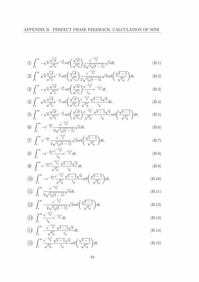
APPENDIX B. PERFECT PHASE FEEDBACK: CALCULATION OF SINR
1
∫ ∞1
−√π
√zt√γxe−
ztγx erf
(√zt√γx
)e− t−1γy
2√γy(t− 1)
√πdt, (B.1)
2
∫ ∞1
√π
√zt√γxe−
ztγx erf
(√zt√γx
)e− t−1γy
2√γy(t− 1)
√πerf
(√t− 1√γy
)dt, (B.2)
3
∫ ∞1
−√π
√zt√γxe−
ztγx erf
(√zt√γx
)e− t−1γy
γye− t−1γy dt, (B.3)
4
∫ ∞1
√π
√zt√γxe−
ztγx erf
(√zt√γx
)e− t−1γy
√γy
√t− 1
√π
γydt, (B.4)
5
∫ ∞1
−√π
√zt√γxe−
ztγx erf
(√zt√γx
)e− t−1γy
√γy
√t− 1
√π
γyerf
(√t− 1√γy
)dt, (B.5)
6
∫ ∞1
−e−2ztγx
e− t−1γy
2√γy(t− 1)
√πdt, (B.6)
7
∫ ∞1
e−2ztγx
e− t−1γy
2√γy(t− 1)
√πerf
(√t− 1√γy
)dt, (B.7)
8
∫ ∞1
−e−2ztγxe− t−1γy
γye− t−1γy dt, (B.8)
9
∫ ∞1
e−2ztγxe− t−1γy
√γy
√t− 1
√π
γydt, (B.9)
10
∫ ∞1
−e−2ztγxe− t−1γy
√γy
√t− 1
√π
γyerf
(√t− 1√γy
)dt, (B.10)
11
∫ ∞1
e− t−1γy
2√γy(t− 1)
√πdt, (B.11)
12
∫ ∞1
− e− t−1γy
2√γy(t− 1)
√πerf
(√t− 1√γy
)dt, (B.12)
13
∫ ∞1
e− t−1γy
γye− t−1γy dt, (B.13)
14
∫ ∞1
−e− t−1γy
√γy
√t− 1
√π
γydt, (B.14)
15
∫ ∞1
e− t−1γy
√γy
√t− 1
√π
γyerf
(√t− 1√γy
)dt. (B.15)
84

The results obtained were:
az = 1 +γxzγy
, bz =z
γx, cz =
γxzγy
, ki =(−1)i
i!(2i+ 1), (B.16)
1 = −√πΓ
(1
2
)e
1γy
∞∑n=0
kn a−n+ 5
22
z bn+ 1
22
z c12z e
−azbz2 Wn+ 3
22
,−n− 3
22
(azbz
), (B.17)
2 = 2 · e1γy
∞∑n=0
∞∑m=0
kn km a−n+m+3
2z b
n+m+12
z cm+1z Γ(m+ 1) e
−az bz2 Wn−m+1
2,−n−m−2
2
(azbz
), (B.18)
3 = −2 e−bz∞∑n=0
n+1∑m=0
kn (n+ 1)! bmz czm! (1 + 2cz)n−m+2
, (B.19)
4 = 2√π Γ
(3
2
)e
1γy
∞∑n=0
kn a−n+ 7
22
z bn+ 3
22
z c32z e
−az bz2 Wn+ 1
22
,−n− 5
22
(azbz
), (B.20)
5 = −4e1γy
∞∑n=0
∞∑m=0
kn km a−n+m+4
2z b
n+m+22
z cm+2z Γ(m+ 2) e
−az bz2 Wn−m
2,−n−m−3
2
(azbz
), (B.21)
6 = −π2e−2bz√1 + 2
cz
, (B.22)
7 =
e−2bz
(π − 2 tan−1
(√1 + 2
cz
))2√
1 + 2cz
, (B.23)
8 = − e−2bz
2(1 + 1cz
), (B.24)
9 =πe−2bz
2(1 + 2cz
)32
, (B.25)
10 = −e−2bz
(π
2(1 + 2cz
)32
−tan−1
(√1 + 2
cz
)(1 + 2
cz)
32
+1
2(1 + 2cz
)(2 + 2cz
)
), (B.26)
11 =π
2, (B.27)
12 = −π4, (B.28)
13 =1
2, (B.29)
14 = −π2, (B.30)
15 =π
4+
1
2. (B.31)
85
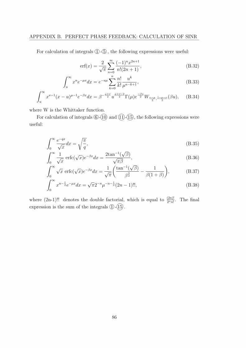
APPENDIX B. PERFECT PHASE FEEDBACK: CALCULATION OF SINR
For calculation of integrals 1 - 5 , the following expressions were useful:
erf(x) =2√π
∞∑n=0
(−1)nx2n+1
n!(2n+ 1), (B.32)∫ ∞
u
xne−µxdx = e−uµn∑k=0
n!
k!
uk
µn−k+1, (B.33)∫ ∞
u
xν−1(x− u)µ−1e−βxdx = β−µ+ν
2 uµ+ν−2
2 Γ(µ)e−βu
2 W ν−µ2, 1−µ−ν
2(βu), (B.34)
where W is the Whittaker function.
For calculation of integrals 6 - 10 and 11 - 15 , the following expressions were
useful:
∫ ∞0
e−qx√xdx =
√π
q, (B.35)∫ ∞
0
1√x
erfc(√x)e−βxdx =
2tan−1(√β)√
πβ, (B.36)∫ ∞
0
√x erfc(
√x)e−βxdx =
1√π
(tan−1(
√β)
β32
− 1
β(1 + β)
), (B.37)∫ ∞
0
xn−12 e−µxdx =
√π2−nµ−n−
12 (2n− 1)!!, (B.38)
where (2n-1)!! denotes the double factorial, which is equal to (2n)!2nn!
. The final
expression is the sum of the integrals 1 - 15 .
86