S1

Electronic Supporting Information

All-Atom Lipid Bilayer Self-Assembly with the

AMBER and Charmm Lipid Force FieldsÅ. A. Skjevik,a,b B. D. Madej,a,d C. J. Dickson,c K. Teigen,b R. C. Walker a,d,* and I. R. Gouldc,*

a San Diego Supercomputer Center, University of California San Diego, 9500 Gilman Drive MC0505, La Jolla, California, 92093-0505, United States.

b Department of Biomedicine, University of Bergen, N-5009 Bergen, Norway.

c Department of Chemistry and Institute of Chemical Biology, Imperial College London, South Kensington, SW7 2AZ, United Kingdom.

d Department of Chemistry and Biochemistry, University of California San Diego, 9500 Gilman Drive MC0505, La Jolla, California, 92093-0505, United States.

Electronic Supplementary Material (ESI) for ChemComm.This journal is © The Royal Society of Chemistry 2015

S2

CONTENTS

METHODS

Simulation details

Self-assembly simulations

Trajectory analyses

SUPPORTING TABLES

Supporting Table 1: Simulation system details

Supporting Table 2: Additional average structural properties calculated for the self-

assembled Lipid14 and C36 bilayers and comparison with experiment

SUPPORTING FIGURES

Supporting Figure 1: Atomic point charges in the PC head group in Lipid14 and

corresponding C36 charges

Supporting Figure 2: Atomic point charges in the PE head group in Lipid14 and

corresponding C36 charges

Supporting Figure 3: C36 DPPC self-assembly

CAPTIONS FOR SUPPORTING VIDEOS

REFERENCES

S3

METHODS

Simulation details. All simulations were run using the GPU/CUDA-accelerated implementation

of AMBER PMEMD (Version 14.0)1, 2 from AMBER 143, 4. Periodic boundary conditions were

applied, with the electrostatic interactions evaluated by means of particle mesh Ewald (PME)

summation5 with 4th order B-spline interpolation and grid spacings of 1.0 Å. A cut-off of 10 Å

limited the direct space sum and truncated the van der Waals interactions. Bonds involving

hydrogen were subjected to length constraints provided by the SHAKE algorithm6. The Langevin

coupling scheme7, with a collision frequency of 1.0 ps-1, regulated temperature while a Berendsen

barostat8 maintained a reference pressure set to 1.0 bar. All simulations utilized the hybrid SPFP

precision model of Le Grand and Walker9.

Self-assembly simulations. Three repeats with Lipid14 parameters were conducted for each of

the four lipid systems in Supporting Table 1 (POPC, DOPC, POPE and DPPC), starting from the

same initial random configuration of lipid, water and ions, but using different random seeds for

each repeat. After a 10,000-step minimization, the following simulation protocol was followed: i)

10 ns simulation at production temperature with 0.5 fs time step and isotropic pressure coupling

(NPT) using initial velocities generated from a Boltzmann distribution; ii) 10 ns simulation at

production temperature with 1.0 fs time step and isotropic pressure coupling (NPT); iii)

Simulation at production temperature with 2.0 fs time step and anisotropic pressure coupling

(NPT). The production temperature was maintained across all three steps, above the phase

transition temperature of the simulated phospholipid (see Supporting Table 1 for specific

temperatures). The simulation parameters applied in step iii) are identical to those used in the

production phase of the Lipid14 parameter validation simulations10.

S4

Equivalent systems as listed in Supporting Table 1, with the same number of lipids,

waters and ions, were generated with the Charmm C36 force field11 and converted to AMBER

topology and coordinate files using CHAMBER12. In three simulation repeats per lipid, the same

procedure as for the Lipid14 systems was followed and the same simulation settings applied.

Trajectory analyses. Since asymmetric lipid distribution was observed in most of the

simulations (Table 1) the areas per lipid were calculated by doubling the lateral area of the

assembled bilayer and dividing by the total number of phospholipids in the system. The volume

per lipid (VL) was derived using the volume of the simulation box (Vbox), the number of water (nw)

and lipid (nlipid) molecules and the temperature-specific volume of a TIP3P water molecule (Vw)10,

13:

box w wL

lipid

V n VVn

Bilayer thickness (DHH) was obtained as the distance between the maxima (i.e. the

phosphate peaks) of the time-averaged electron density profile, while the Luzzati thickness was

calculated by subtracting the integral of the water density probability distribution (ρw(bn)) along

the bilayer normal dimension (bn) from the time-averaged bilayer normal dimension dbn10, 14, 15:

/2

/2( )bn

B bn w bnbn

d

dD d bn d

Isothermal compressibility moduli (KA) were obtained through the following equation10,

13:

2 B LA

lipid

k T AK

n A

S5

T is the temperature, kB is the Boltzmann constant, <AL> refers to the mean area per lipid and σA2

corresponds to the area per lipid variance.

The lateral diffusion coefficient (D) was computed as the slope of the plot of the mean

square displacement (MSD) of the lipids versus time t (the number of dimensions, n, is equal to 2

for lateral diffusion in bilayers):

lim2t

MSDDnt

Any centre of mass drift of each bilayer leaflet was removed from the trajectories before

calculating the average MSD over a large number of 20 ns windows of different time origin, with

200 ps separating the time origins of sequentially analyzed windows. The last 100 ns of each

simulation was used for the MSD calculation, and the linear 10-20 ns portion of the resulting

curve was used for deriving the slope via linear regression10.

The bulk of the analyses described above was carried out using PTRAJ/CPPTRAJ3, 16, and

the snapshots in Figure 1 were generated using VMD17.

S6

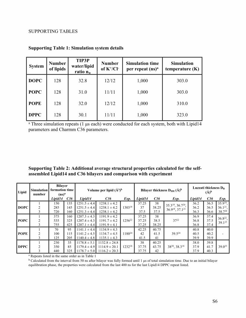
SUPPORTING TABLES

Supporting Table 1: Simulation system details

System Number of lipids

TIP3P water/lipid

ratio nw

Number of K+/Cl-

Simulation time per repeat (ns)a

Simulation temperature (K)

DOPC 128 32.8 12/12 1,000 303.0

POPC 128 31.0 11/11 1,000 303.0

POPE 128 32.0 12/12 1,000 310.0

DPPC 128 30.1 11/11 1,000 323.0a Three simulation repeats (1 μs each) were conducted for each system, both with Lipid14 parameters and Charmm C36 parameters.

Supporting Table 2: Additional average structural properties calculated for the self-assembled Lipid14 and C36 bilayers and comparison with experiment

a Repeats listed in the same order as in Table 1b Calculated from the interval from 50 ns after bilayer was fully formed until 1 μs of total simulation time. Due to an initial bilayer equilibration phase, the properties were calculated from the last 400 ns for the last Lipid14 DPPC repeat listed.

Bilayer formation time

(ns)aVolume per lipid (Å3)b Bilayer thickness DHH (Å)b Luzzati thickness DB

(Å)bLipid Simulation number

Lipid14 C36 Lipid14 C36 Exp. Lipid14 C36 Exp. Lipid14 C36 Exp.1 150 135 1251.5 ± 4.4 1238.1 ± 4.2 37.25 38 36.2 36.52 285 145 1251.5 ± 4.4 1238.1 ± 4.2 37 38.25 36.2 36.5DOPC3 720 160 1251.3 ± 4.4 1238.1 ± 4.2

130318

37.5 37.5

35.319, 36.720, 36.918, 37.121

36.3 36.6

35.918, 36.121, 38.720

1 375 160 1207.3 ± 4.3 1191.9 ± 4.2 37.25 38 36.9 37.42 535 325 1207.4 ± 4.3 1191.7 ± 4.2 37.25 38.5 36.8 37.5POPC3 755 425 1207.1 ± 4.4 1191.9 ± 4.1

125622

37.25 38.253722

36.8 37.4

36.822, 39.123

1 70 95 1141.1 ± 4.4 1134.9 ± 4.3 42.25 40.75 40.8 40.02 100 115 1141.2 ± 4.5 1134.7 ± 4.5 42 41.5 40.5 40.2POPE3 125 205 1140.4 ± 4.8 1135.1 ± 4.3

118024

41.5 4139.524

39.9 39.9-

1 230 35 1178.8 ± 5.1 1132.8 ± 24.8 38 40.25 38.0 39.82 350 85 1179.4 ± 4.9 1114.9 ± 20.1 37.75 43.75 37.9 41.7DPPC3 440 325 1178.7 ± 5.0 1116.2 ± 20.3

123218

37.75 423820, 38.318

37.9 40.339.023

S7

Supporting Figure 1. Atomic point charges in the PC head group in Lipid14 (taken from lipid14.lib) with corresponding C36 charges in parentheses (taken from top_all36_lipid.rtf).

S8

Supporting Figure 2. Atomic point charges in the PE head group in Lipid14 (taken from lipid14.lib) with corresponding C36 charges in parentheses (taken from top_all36_lipid.rtf).

S9

0 ns 36 ns

85 ns 270 ns

560 ns 1000 ns

Supporting Figure 1. C36 DPPC self-assembly. The snapshots are taken from the first simulation listed in Table 1 and are representative of all three repeats (though with different timings). The lipids eventually adopt a highly ordered configuration, where tails from opposite leaflets completely overlap in parts of the membrane (after 560, 600 and 700 ns for the three repeats, respectively). This configuration is very stable for the remainder of the simulation.

S10

CAPTIONS FOR SUPPORTING VIDEOS

Supporting Video 1: DOPC self-assembly. The video shows the first 250 ns of the first Lipid14

DOPC self-assembly simulation listed in Table 1, with a simulation time interval of 200 ps

between frames. The lipids are represented as line models coloured by element, with the head

group phosphorus atoms highlighted as orange spheres. Water, ions and hydrogens have been

removed for clarity.

Supporting Video 2: POPC self-assembly. The video shows the first 475 ns of the first Lipid14

POPC self-assembly simulation listed in Table 1, with a simulation time interval of 200 ps

between frames. The lipids are represented as line models coloured by element, with the head

group phosphorus atoms highlighted as orange spheres. Water, ions and hydrogens have been

removed for clarity.

Supporting Video 3: POPE self-assembly. The video shows the first 200 ns of the second

Lipid14 POPE self-assembly simulation listed in Table 1, with a simulation time interval of 200

ps between frames. The lipids are represented as line models coloured by element, with the head

group phosphorus atoms highlighted as orange spheres. Water, ions and hydrogens have been

removed for clarity.

Supporting Video 4: DPPC self-assembly. The video shows the first 700 ns of the third Lipid14

DPPC self-assembly simulation listed in Table 1, with a simulation time interval of 200 ps

between frames. The lipids are represented as line models coloured by element, with the head

group phosphorus atoms highlighted as orange spheres. Water, ions and hydrogens have been

removed for clarity.

S11

REFERENCES

1. A. W. Götz, M. J. Williamson, D. Xu, D. Poole, S. Le Grand and R. C. Walker, J. Chem. Theory Comput., 2012, 8, 1542-1555.

2. R. Salomon-Ferrer, A. W. Götz, D. Poole, S. Le Grand and R. C. Walker, J. Chem. Theory Comput., 2013, 9, 3878-3888.

3. D. A. Case, V. Babin, J. T. Berryman, R. M. Betz, Q. Cai, D. S. Cerutti, T. E. Cheatham, III, T. A. Darden, R. E. Duke, H. Gohlke, A. W. Götz, S. Gusarov, N. Homeyer, P. Janowski, J. Kaus, I. Kolossváry, A. Kovalenko, T. S. Lee, S. Le Grand, T. Luchko, R. Luo, B. D. Madej, K. M. Merz, F. Paesani, D. R. Roe, A. Roitberg, C. Sagui, R. Salomon-Ferrer, G. Seabra, C. Simmerling, W. Smith, J. Swails, R. C. Walker, J. Wang, R. M. Wolf, X. Wu and P. A. Kollman, AMBER 14, University of California, San Francisco, 2014.

4. R. Salomon-Ferrer, D. A. Case and R. C. Walker, WIREs Comput. Mol. Sci., 2013, 3, 198-210.

5. T. Darden, D. York and L. Pedersen, J. Chem. Phys., 1993, 98, 10089-10092.

6. J.-P. Ryckaert, G. Ciccotti and H. J. C. Berendsen, J. Comput. Phys., 1977, 23, 327-341.

7. R. J. Loncharich, B. R. Brooks and R. W. Pastor, Biopolymers, 1992, 32, 523-535.

8. H. J. C. Berendsen, J. P. M. Postma, W. F. van Gunsteren, A. DiNola and J. R. Haak, J. Chem. Phys., 1984, 81, 3684-3690.

9. S. Le Grand, A. W. Götz and R. C. Walker, Comput. Phys. Commun., 2013, 184, 374-380.

10. C. J. Dickson, B. D. Madej, Å. A. Skjevik, R. M. Betz, K. Teigen, I. R. Gould and R. C. Walker, J. Chem. Theory Comput., 2014, 10, 865-879.

11. J. B. Klauda, R. M. Venable, J. A. Freites, J. W. O'Connor, D. J. Tobias, C. Mondragon-Ramirez, I. Vorobyov, A. D. MacKerell, Jr. and R. W. Pastor, J. Phys. Chem. B, 2010, 114, 7830-7843.

12. M. F. Crowley, M. J. Williamson and R. C. Walker, Int. J. Quantum Chem., 2009, 109, 3767-3772.

13. C. J. Dickson, L. Rosso, R. M. Betz, R. C. Walker and I. R. Gould, Soft Matter, 2012, 8, 9617-9627.

S12

14. J. P. M. Jämbeck and A. P. Lyubartsev, J. Phys. Chem. B, 2012, 116, 3164-3179.

15. D. Poger, W. F. van Gunsteren and A. E. Mark, J. Comput. Chem., 2010, 31, 1117-1125.

16. D. R. Roe and T. E. Cheatham, III, J. Chem. Theory Comput., 2013, 9, 3084-3095.

17. W. Humphrey, A. Dalke and K. Schulten, J. Mol. Graph., 1996, 14, 33-38.

18. J. F. Nagle and S. Tristram-Nagle, Biochim. Biophys. Acta, 2000, 1469, 159-195.

19. S. Tristram-Nagle, H. I. Petrache and J. F. Nagle, Biophys. J., 1998, 75, 917-925.

20. N. Kučerka, J. F. Nagle, J. N. Sachs, S. E. Feller, J. Pencer, A. Jackson and J. Katsaras, Biophys. J., 2008, 95, 2356-2367.

21. Y. Liu and J. F. Nagle, Phys Rev E, 2004, 69, 040901.

22. N. Kučerka, S. Tristram-Nagle and J. F. Nagle, J. Membr. Biol., 2005, 208, 193-202.

23. N. Kučerka, M.-P. Nieh and J. Katsaras, Biochim. Biophys. Acta, 2011, 1808, 2761-2771.

24. M. Rappolt, A. Hickel, F. Bringezu and K. Lohner, Biophys. J., 2003, 84, 3111-3122.