american community survey multiyear accuracy of the … · american community survey office page 1...

9/19/2011 American Community Survey Office

of 28

American Community Survey Multiyear Accuracy of the Data

(3-year 2008-2010 and 5-year 2006-2010) INTRODUCTION This multiyear ACS Accuracy of the Data document pertains to both the 2008-2010 3-year ACS data products and the 2006-2010 5-year ACS data products. Differences will be noted where applicable. The data contained in these data products are based on the American Community Survey (ACS) sample. For the 3-year data products interviews from January 1, 2008 through December 31, 2010 were used. For the 5-year data products, interviews from January 1, 2006 through December 31, 2010 were used. Data products were produced for 1-year estimates (2006, 2007, 2008, 2009 and 2010), in addition to this set of 3-year and 5-year estimates. In general, ACS estimates are period estimates that describe the average characteristics of population and housing over a period of data collection. The 2008-2010 ACS estimates are averages over the period from January 1, 2008 to December 31, 2010, and the 2006-2010 ACS estimates from January 1, 2006 through December 31, 2010, respectively. Multiyear estimates cannot be used to say what is going on in any particular year in the period, only what the average value is over the full period. The ACS sample is selected from all counties and county-equivalents in the United States. In 2006, the ACS began collection of data from sampled persons in group quarters (GQ) – for example, military barracks, college dormitories, nursing homes, and correctional facilities. Persons in group quarters are included with persons in housing units (HUs) in all 2008-2010 and 2006-2010 ACS estimates based on the total population. The ACS, like any other statistical activity, is subject to error. The purpose of this documentation is to provide data users with a basic understanding of the ACS sample design, estimation methodology, and accuracy of the 2008-2010 and 2006-2010 ACS estimates. The ACS is sponsored by the U.S. Census Bureau, and is part of the 2010 Decennial Census Program. Additional information on the design and methodology of the ACS, including data collection and processing, can be found at http://www.census.gov/acs/www/methodology/methodology_main/ The Multiyear Accuracy of the Data from the Puerto Rico Community Survey can be found at http://www.census.gov/acs/www/data_documentation/documentation_main/

http://www.census.gov/acs/www/methodology/methodology_main/


of 28

Table of Contents

INTRODUCTION .......................................................................................................................... 1 DATA COLLECTION ................................................................................................................... 3 SAMPLE DESIGN ......................................................................................................................... 3 WEIGHTING METHODOLOGY .................................................................................................. 5 ESTIMATION METHODOLOGY FOR MULTIYEAR ESTIMATES ........................................ 6 CONFIDENTIALITY OF THE DATA .......................................................................................... 7 ERRORS IN THE DATA ............................................................................................................... 8 MEASURES OF SAMPLING ERROR ......................................................................................... 9 CALCULATION OF STANDARD ERRORS ............................................................................. 10

Sums and Differences of Direct Standard Errors ...................................................................... 11 Ratios ........................................................................................................................................ 12 Proportions/Percents ................................................................................................................. 12 Percent Change ......................................................................................................................... 12 Products..................................................................................................................................... 13 Differences of Estimates for Overlapping Periods of Identical Length .................................... 13

TESTING FOR SIGNIFICANT DIFFERENCES ........................................................................ 13 EXAMPLES OF STANDARD ERROR CALCULATIONS....................................................... 14 CONTROL OF NONSAMPLING ERROR ................................................................................. 17 ISSUES WITH APPROXIMATING THE STANDARD ERROR OF LINEAR COMBINATIONS OF MULTIPLE ESTIMATES ...................................................................... 21


of 28

DATA COLLECTION The ACS employs three modes of data collection:

• Mailout/Mailback • Computer Assisted Telephone Interview (CATI) • Computer Assisted Personal Interview (CAPI)

The general timing of data collection is: Month 1: Addresses determined to be mailable are sent a questionnaire via the U.S. Postal

Service. Month 2: All mail non-responding addresses with an available phone number are sent to

CATI. Month 3: A sample of mail non-responses without a phone number, CATI non-responses,

and unmailable addresses are selected and sent to CAPI. SAMPLE DESIGN Sampling rates are assigned independently at the census block level. A measure of size is calculated for each of the following governmental units:

• Counties • Places (active, functioning governmental units) • School Districts (elementary, secondary, and unified) • American Indian Areas (including Tribal Subdivisions beginning in 2008) • Minor Civil Divisions (MCDs) – Connecticut, Maine, Massachusetts, Michigan,

Minnesota, New Hampshire, New Jersey, New York, Pennsylvania, Rhode Island, Vermont, and Wisconsin (these are the states where MCDs are active, functioning governmental units)

• Alaska Native Village Statistical Areas • Hawaiian Homelands

Each block is then assigned the smallest measure of size (GUMOS) from the set of all governmental units it is a part of. The measure of size for all geographic entities for all areas (except American Indian Areas) is an estimate of the number of occupied housing units in the area. This was calculated by multiplying the number of ACS addresses by an estimate of the occupancy rate from Census 2000 and the ACS at the block level. For American Indian Areas the measure of size is the estimated number of occupied housing units multiplied by the proportion of people reporting American Indian (alone or in combination) in Census 2000. A measure of size for each census tract (TRACTMOS) was also calculated in the same manner.


of 28

Table 1. 2006 Through 2010 Sampling Rates for the United States

Sampling Rate Category 2006 Sampling

Rates

2007 Sampling

Rates

2008 Sampling

Rates

2009 Sampling

Rates

2010 Sampling

Rates Blocks in smallest governmental units (GUMOS < 200)

10.0% 10.0% 10.0% 10.0% 10.0%

Blocks in smaller governmental units (200 ≤ GUMOS < 800)

6.8% 6.7% 6.6% 6.5% 6.7%

Blocks in small governmental units (800 ≤ GUMOS ≤ 1200)

3.4% 3.3% 3.3% 3.3% 3.3%

Blocks in large tracts (GUMOS > 1200, TRACTMOS ≥ 2000) where mailable addresses ≥ 75% and predicted levels of completed mail and CATI interviews prior to CAPI subsampling > 60%

1.6% 1.5% 1.5% 1.5% 1.5%

Other blocks in large tracts (GUMOS > 1200, TRACTMOS ≥ 2000)

1.7% 1.6% 1.6% 1.6% 1.6%

All other blocks (GUMOS > 1200, TRACTMOS < 2000) where mailable addresses ≥ 75% and predicted levels of completed mail and CATI interviews prior to CAPI subsampling > 60%

2.1% 2.1% 2.0% 2.0% 2.0%

All other blocks (GUMOS > 1200, TRACTMOS < 2000)

2.3% 2.2% 2.2% 2.2% 2.2%

Addresses determined to be unmailable do not go to the CATI phase of data collection and are subsampled for the CAPI phase of data collection at a rate of 2-in-3. Subsequent to CATI, all addresses for which no response has been obtained are subsampled. This subsample is sent to the CAPI data collection phase. Beginning with the CAPI sample for the January 2006 panel (March 2006 data collection), the CAPI subsampling rate was based on the expected rate of completed mail and CATI interviews at the tract level.


of 28

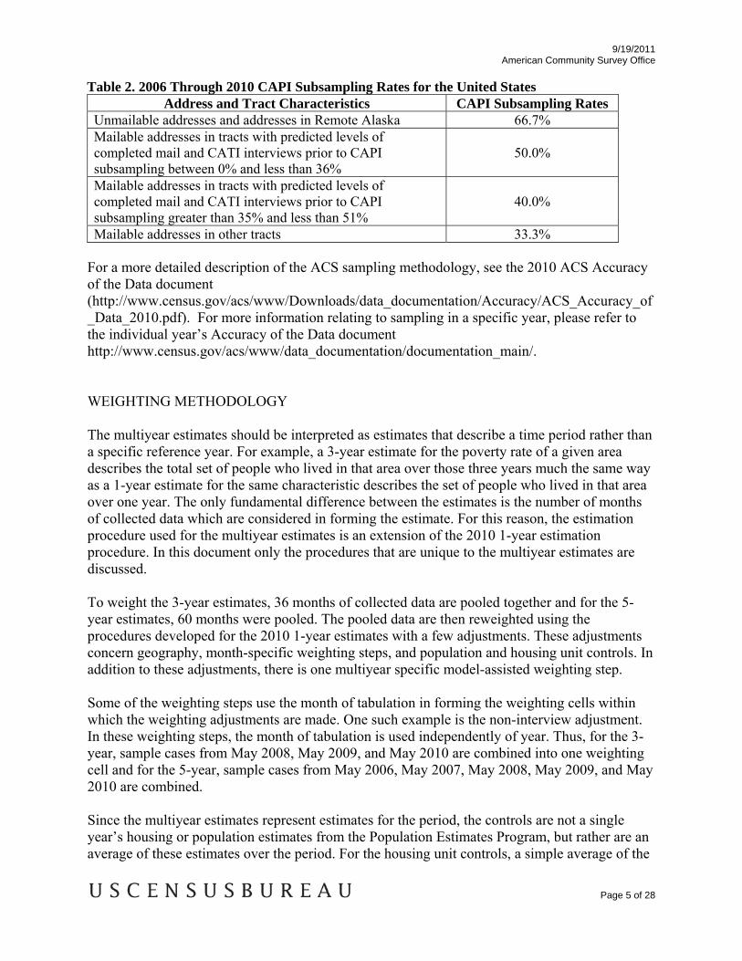
Table 2. 2006 Through 2010 CAPI Subsampling Rates for the United States Address and Tract Characteristics CAPI Subsampling Rates

Unmailable addresses and addresses in Remote Alaska 66.7% Mailable addresses in tracts with predicted levels of completed mail and CATI interviews prior to CAPI subsampling between 0% and less than 36%

50.0%

Mailable addresses in tracts with predicted levels of completed mail and CATI interviews prior to CAPI subsampling greater than 35% and less than 51%

40.0%

Mailable addresses in other tracts 33.3% For a more detailed description of the ACS sampling methodology, see the 2010 ACS Accuracy of the Data document (http://www.census.gov/acs/www/Downloads/data_documentation/Accuracy/ACS_Accuracy_of_Data_2010.pdf). For more information relating to sampling in a specific year, please refer to the individual year’s Accuracy of the Data document http://www.census.gov/acs/www/data_documentation/documentation_main/. WEIGHTING METHODOLOGY The multiyear estimates should be interpreted as estimates that describe a time period rather than a specific reference year. For example, a 3-year estimate for the poverty rate of a given area describes the total set of people who lived in that area over those three years much the same way as a 1-year estimate for the same characteristic describes the set of people who lived in that area over one year. The only fundamental difference between the estimates is the number of months of collected data which are considered in forming the estimate. For this reason, the estimation procedure used for the multiyear estimates is an extension of the 2010 1-year estimation procedure. In this document only the procedures that are unique to the multiyear estimates are discussed. To weight the 3-year estimates, 36 months of collected data are pooled together and for the 5-year estimates, 60 months were pooled. The pooled data are then reweighted using the procedures developed for the 2010 1-year estimates with a few adjustments. These adjustments concern geography, month-specific weighting steps, and population and housing unit controls. In addition to these adjustments, there is one multiyear specific model-assisted weighting step. Some of the weighting steps use the month of tabulation in forming the weighting cells within which the weighting adjustments are made. One such example is the non-interview adjustment. In these weighting steps, the month of tabulation is used independently of year. Thus, for the 3-year, sample cases from May 2008, May 2009, and May 2010 are combined into one weighting cell and for the 5-year, sample cases from May 2006, May 2007, May 2008, May 2009, and May 2010 are combined. Since the multiyear estimates represent estimates for the period, the controls are not a single year’s housing or population estimates from the Population Estimates Program, but rather are an average of these estimates over the period. For the housing unit controls, a simple average of the


of 28

1-year housing unit estimates over the period is calculated for each county or subcounty area. The version or vintage of estimates used is always the last year of the period since these are considered to be the most up-to-date and are created using a consistent methodology. For example, the housing unit control used for a given county in the 2006-2010 weighting is equal to the simple average of the 2006, 2007, 2008, 2009, and 2010 estimates that were produced using the 2010 methodology (the 2010 vintage). Likewise, the population controls by race, ethnicity, age, and sex are obtained by taking a simple average of the 1-year population estimates of the county or weighting area by race, ethnicity, age, and sex. For example, the 2006-2010 control total used for Hispanic males age 20-24 in a given county would be obtained by averaging the 1-year population estimates for that demographic group for 2006, 2007, 2008, 2009, and 2010. The version or vintage of estimates used is always that of the last year of the period since these are considered to be the most up to date and are created using a consistent methodology. One multiyear specific step is a model-assisted (generalized regression or GREG) weighting step. The objective of this additional step is to reduce the variances of base demographics at the place and MCD level in the 3-year estimates and at the tract level in the 5-year estimates. While reducing the variances, the estimates themselves are relatively unchanged. This process involves linking administrative record data with ACS data. In addition, a finite population correction (FPC) factor is included in the creation of the replicate weights for both the 3-year and 5-year data at the tract level. It reduces the estimate of the variance and the margin of error by taking the sampling rate into account. A two-tiered approach was used. One FPC was calculated for mail and CATI respondents and another for CAPI respondents. The CAPI was given a separate FPC to take into account the fact that CAPI respondents are subsampled. The FPC is not included in the 1-year data because the sampling rates are relatively small and thus the FPC does not have an appreciable impact on the variance. For more information on the replicate weights and replicate factors, see the Design and Methodology Report located at http://www.census.gov/acs/www/methodology/methodology_main/. ESTIMATION METHODOLOGY FOR MULTIYEAR ESTIMATES For the 1-year estimation, the tabulation geography for the data is based on the boundaries defined on January 1 of the tabulation year, which is consistent with the tabulation geography used to produce the population estimates. All sample addresses are updated with this geography prior to weighting. For the multiyear estimation, the tabulation geography for the data is referenced to the final year in the multiyear period. For example, the 2008-2010 period uses the 2010 reference geography. Thus, all data collected over the period of 2008-2010 in the blocks that are contained in the 2010 boundaries for a given place are tabulated as though they were a part of that place for the entire period. Monetary values for the ACS 3-year estimates are inflation-adjusted to the final year of the period. For example, the 2008-2010 ACS 3-year estimates are tabulated using 2010-adjusted dollars. These adjustments use the national Consumer Price Index (CPI) since a regional-based


of 28

CPI is not available for the entire country. The ACS 5-year estimates are also inflation-adjusted in the same manner. For a more detailed description of the ACS estimation methodology, see the 2010 Accuracy of the Data document (http://www.census.gov/acs/www/Downloads/data_documentation/Accuracy/ACS_Accuracy_of_Data_2010.pdf). For more information relating to estimation in a specific year, please refer to that individual year’s Accuracy of the Data document (http://www.census.gov/acs/www/data_documentation/documentation_main/). CONFIDENTIALITY OF THE DATA The Census Bureau has modified or suppressed some data on this site to protect confidentiality. Title 13 United States Code, Section 9, prohibits the Census Bureau from publishing results in which an individual's data can be identified. The Census Bureau’s internal Disclosure Review Board sets the confidentiality rules for all data releases. A checklist approach is used to ensure that all potential risks to the confidentiality of the data are considered and addressed.

• Title 13, United States Code: Title 13 of the United States Code authorizes the Census Bureau to conduct censuses and surveys. Section 9 of the same Title requires that any information collected from the public under the authority of Title 13 be maintained as confidential. Section 214 of Title 13 and Sections 3559 and 3571 of Title 18 of the United States Code provide for the imposition of penalties of up to five years in prison and up to $250,000 in fines for wrongful disclosure of confidential census information.

• Disclosure Limitation: Disclosure limitation is the process for protecting the

confidentiality of data. A disclosure of data occurs when someone can use published statistical information to identify an individual that has provided information under a pledge of confidentiality. For data tabulations the Census Bureau uses disclosure limitation procedures to modify or remove the characteristics that put confidential information at risk for disclosure. Although it may appear that a table shows information about a specific individual, the Census Bureau has taken steps to disguise or suppress the original data while making sure the results are still useful. The techniques used by the Census Bureau to protect confidentiality in tabulations vary, depending on the type of data.

• Data Swapping: Data swapping is a method of disclosure limitation designed to protect

confidentiality in tables of frequency data (the number or percent of the population with certain characteristics). Data swapping is done by editing the source data or exchanging records for a sample of cases when creating a table. A sample of households is selected and matched on a set of selected key variables with households in neighboring geographic areas that have similar characteristics (such as the same number of adults and same number of children). Because the swap often occurs within a neighboring area,


of 28

there is no effect on the marginal totals for the area or for totals that include data from multiple areas. Because of data swapping, users should not assume that tables with cells having a value of one or two reveal information about specific individuals. Data swapping procedures were first used in the 1990 Census, and were used again in Census 2000 and the 2010 Census.

The data use the same disclosure limitation methodology as the original 1-year data. The confidentiality edit was previously applied to the raw data files when they were created to produce the 1-year estimates and these same data files with the original confidentiality edit were used to produce the 3-year and 5-year estimates. ERRORS IN THE DATA

• Sampling Error — The data in the ACS products are estimates of the actual figures that would have been obtained by interviewing the entire population using the same methodology. The estimates from the chosen sample also differ from other samples of housing units and persons within those housing units. Sampling error in data arises due to the use of probability sampling, which is necessary to ensure the integrity and representativeness of sample survey results. The implementation of statistical sampling procedures provides the basis for the statistical analysis of sample data.

• Nonsampling Error — In addition to sampling error, data users should realize that other

types of errors may be introduced during any of the various complex operations used to collect and process survey data. For example, operations such as data entry from questionnaires and editing may introduce error into the estimates. Another source is through the use of controls in the weighting. The controls are designed to mitigate the effects of systematic undercoverage of certain groups who are difficult to enumerate and to reduce the variance. The controls are based on the population estimates extrapolated from the previous census. Errors can be brought into the data if the extrapolation methods do not properly reflect the population. However, the potential risk from using the controls in the weighting process is offset by far greater benefits to the ACS estimates. These benefits include reducing the effects of a larger coverage problem found in most surveys, including the ACS, and the reduction of standard errors of ACS estimates. These and other sources of error contribute to the nonsampling error component of the total error of survey estimates. Nonsampling errors may affect the data in two ways. Errors that are introduced randomly increase the variability of the data. Systematic errors which are consistent in one direction introduce bias into the results of a sample survey. The Census Bureau protects against the effect of systematic errors on survey estimates by conducting extensive research and evaluation programs on sampling techniques, questionnaire design, and data collection and processing procedures. In addition, an important goal of the ACS is to minimize the amount of nonsampling error introduced through nonresponse for sample housing units. One way of accomplishing this is by following up on mail nonrespondents during the CATI and CAPI phases.


of 28

MEASURES OF SAMPLING ERROR Sampling error is the difference between an estimate based on a sample and the corresponding value that would be obtained if the estimate were based on the entire population (as from a census). Note that sample-based estimates will vary depending on the particular sample selected from the population. Measures of the magnitude of sampling error reflect the variation in the estimates over all possible samples that could have been selected from the population using the same sampling methodology. Estimates of the magnitude of sampling errors – in the form of margins of error – are provided with all published ACS estimates. The Census Bureau recommends that data users incorporate this information into their analyses, as sampling error in survey estimates could impact the conclusions drawn from the results. Confidence Intervals and Margins of Error Confidence Intervals – A sample estimate and its estimated standard error may be used to construct confidence intervals about the estimate. These intervals are ranges that will contain the average value of the estimated characteristic that results over all possible samples, with a known probability.

For example, if all possible samples that could result under the ACS sample design were independently selected and surveyed under the same conditions, and if the estimate and its estimated standard error were calculated for each of these samples, then:

1. Approximately 68 percent of the intervals from one estimated standard error below

the estimate to one estimated standard error above the estimate would contain the average result from all possible samples;

2. Approximately 90 percent of the intervals from 1.645 times the estimated standard

error below the estimate to 1.645 times the estimated standard error above the estimate would contain the average result from all possible samples.

3. Approximately 95 percent of the intervals from two estimated standard errors below

the estimate to two estimated standard errors above the estimate would contain the average result from all possible samples.

The intervals are referred to as 68 percent, 90 percent, and 95 percent confidence intervals, respectively. Margin of Error – Instead of providing the upper and lower confidence bounds in published ACS tables, the margin of error is provided instead. The margin of error is the difference between an estimate and its upper or lower confidence bound. Both the confidence bounds and the standard error can easily be computed from the margin of error. All ACS published margins of error are based on a 90 percent confidence level.


of 28

Standard Error = Margin of Error / 1.645

Lower Confidence Bound = Estimate - Margin of Error

Upper Confidence Bound = Estimate + Margin of Error When constructing confidence bounds from the margin of error, the user should be aware of any “natural” limits on the bounds. For example, if a population estimate is near zero, the calculated value of the lower confidence bound may be negative. However, a negative number of people does not make sense, so the lower confidence bound should be reported as zero instead. However, for other estimates such as income, negative values do make sense. The context and meaning of the estimate must be kept in mind when creating these bounds. Another of these natural limits would be 100% for the upper bound of a percent estimate. If the margin of error is displayed as ‘*****’ (five asterisks), the estimate has been controlled to be equal to a fixed value and so has no sampling error. When using any of the formulas in the following section, use a standard error of zero for these controlled estimates. Limitations –The user should be careful when computing and interpreting confidence intervals.

• The estimated standard errors (and thus margins of errors) included in these data products do not include portions of the variability due to nonsampling error that may be present in the data. In particular, the standard errors do not reflect the effect of correlated errors introduced by interviewers, coders, or other field or processing personnel. Nor do they reflect the error from imputed values due to missing responses. Thus, the standard errors calculated represent a lower bound of the total error. As a result, confidence intervals formed using these estimated standard errors may not meet the stated levels of confidence (i.e., 68, 90, or 95 percent). Thus, some care must be exercised in the interpretation of the data in this data product based on the estimated standard errors.

• Zero or small estimates; very large estimates — The value of almost all ACS

characteristics is greater than or equal to zero by definition. For zero or small estimates, use of the method given previously for calculating confidence intervals relies on large sample theory, and may result in negative values which for most characteristics are not admissible. In this case the lower limit of the confidence interval is set to zero by default. A similar caution holds for estimates of totals close to a control total or estimated proportions near one, where the upper limit of the confidence interval is set to its largest admissible value. In these situations the level of confidence of the adjusted range of values is less than the prescribed confidence level.

CALCULATION OF STANDARD ERRORS Direct estimates of the standard errors were calculated for all estimates reported in this product. The standard errors, in most cases, are calculated using a replicate-based methodology that takes into account the sample design and estimation procedures. Excluding the base weight, replicate


of 28

weights were allowed to be negative in order to avoid underestimating the standard error. Exceptions include:

1. The estimate of the number or proportion of people, households, families, or housing units in a geographic area with a specific characteristic is zero. A special procedure is used to estimate the standard error.

2. There are either no sample observations available to compute an estimate or standard

error of a median, an aggregate, a proportion, or some other ratio, or there are too few sample observations to compute a stable estimate of the standard error. The estimate is represented in the tables by “-” and the margin of error by “**” (two asterisks).

3. The estimate of a median falls in the lower open-ended interval or upper open-ended

interval of a distribution. If the median occurs in the lowest interval, then a “-” follows the estimate, and if the median occurs in the upper interval, then a “+” follows the estimate. In both cases the margin of error is represented in the tables by “***” (three asterisks).

Sums and Differences of Direct Standard Errors The standard errors estimated from these tables are for individual estimates. Additional calculations are required to estimate the standard errors for sums of or the differences between two or more sample estimates. The standard error of the sum of two sample estimates is the square root of the sum of the two individual standard errors squared plus a covariance term. That is, for standard errors and of estimates and :

(1)

The covariance measures the interactions between two estimates. Currently the covariance terms are not available. Data users should use the approximation:

(2)

However, this method will underestimate or overestimate the standard error if the two estimates interact in either a positive or negative way. The approximation formula (2) can be expanded to more than two estimates by adding in the individual standard errors squared inside the radical. As the number of estimates involved in the sum or difference increases, the results of formula (2) become increasingly different from the standard error derived directly from the ACS microdata. Users are encouraged to work with the fewest number of estimates possible. If there are estimates involved in the sum that are controlled in the weighting then the approximate standard error can be increasingly different.


of 28

Several examples are provided starting on page 21 to demonstrate issues associated with approximating the standard errors when summing large numbers of estimates together. Ratios The statistic of interest may be the ratio of two estimates. First is the case where the numerator is not a subset of the denominator. The standard error of this ratio between two sample estimates is approximated as:

1 (3)

Proportions/Percents For a proportion (or percent), a ratio where the numerator is a subset of the denominator, a slightly different estimator is used. If ⁄ , then the standard error of this proportion is approximated as:

1 (4)

If 100% (P is the proportion and Q is its corresponding percent), then 100% . Note the difference between the formulas to approximate the standard error for proportions (4) and ratios (3) - the plus sign in the previous formula has been replaced with a minus sign. If the value under the radical is negative, use the ratio standard error formula above, instead. Percent Change Calculating the percent change from one time period to another. For example, computing the percent change of a 2005-2007 estimate to a 2008-2010 estimate. Normally, the current estimate is compared to the older estimate. Let the current estim t and the earlier estimate = Y, then the formula for percent change is: a e = X

100% 100% 1 100%

(5)

This reduces to a ratio. The ratio formula (3) above may be used to calculate the standard error. As a caveat, this formula does not take into account the correlation when calculating overlapping time periods.


of 28

Products For a product of two estimates - for example if you want to estimate a proportion’s numerator by multiplying the proportion by its denominator - the standard error can be approximated as:

(6)

Differences of Estimates for Overlapping Periods of Identical Length For example, may represent an estimate of a characteristic for the period 2007-2009 and the estimate of the same characteristic for 2008-2010. In this case, data for 2008 and 2009 are included in both estimates, and their contribution is largely subtracted out when differences are calculated. In this case, it is possible to approximate the sampling correlation between the two estimates to improve upon the previous expression, namely:

√1 (7)

where C is the fraction of overlapping years. For example, the periods 2007-2009 and 2008-2010 overlap by two out of three years, so C = 2 / 3 and 1 - C = 0.33. If the periods do not overlap, such as 2005-2007 and 2008-2010, then no factor is needed. Due to the difficulty in interpreting overlapping time periods, the Census Bureau currently discourages users from making such comparisons. TESTING FOR SIGNIFICANT DIFFERENCES Significant differences – Users may conduct a statistical test to see if the difference between an ACS estimate and any other chosen estimates is statistically significant at a given confidence level. “Statistically significant” means that the difference is not likely due to random chance alone. With the two estimates (Est1 and Est2) and their respective standard errors (SE1 and SE2), calculate a Z statistic: (8)

If Z > 1.645 or Z < -1.645, then the difference can be said to be statistically significant at the 90 percent confidence level.1 Any estimate can be compared to an ACS estimate using this method, including other ACS estimates from the current year, the ACS estimate for the same characteristic and geographic area but from a previous year, Census 2010 counts, Census 2000 100 percent counts and long form estimates, estimates from other Census Bureau surveys, and estimates from other sources. Not all estimates have sampling error — Census 2010 counts and Census 2000 100 percent counts do not, for example, although Census 2000 long form estimates do — but they should be used if they exist to give the most accurate result of the test.

1 The ACS Accuracy of the Data document in 2005 used a Z statistic of +/-1.65. Data users should use +/-1.65 for estimates published in 2005 or earlier.


of 28

Users are also cautioned to not rely on looking at whether confidence intervals for two estimates overlap or not to determine statistical significance, because there are circumstances where that method will not give the correct test result. If two confidence intervals do not overlap, then the estimates will be significantly different (i.e. the significance test will always agree). However, if two confidence intervals do overlap, then the estimates may or may not be significantly different. The Z calculation above is recommended in all cases.

Here is a simple example of why it is not recommended to use the overlapping confidence bounds rule of thumb as a substitute for a statistical test.

Let: X1 = 6.0 with SE1 = 0.5 and X2 = 5.0 with SE2 = 0.2. The Lower Bound for X1 = 6.0 - 0.5 * 1.645 = 5.2 while the Upper Bound for X2 = 5.0 - 0.2 * 1.645 = 5.3. The confidence bounds overlap, so, the rule of thumb would indicate that the estimates are not significantly different at the 90% level. However, if we apply the statistical significance test we obtain:

6 5

√0.5 0.21.857

Z = 1.857 > 1.645 which means that the difference is significant (at the 90% level).

All statistical testing in ACS data products is based on the 90 percent confidence level. Users should understand that all testing was done using unrounded estimates and standard errors, and it may not be possible to replicate test results using the rounded estimates and margins of error as published. EXAMPLES OF STANDARD ERROR CALCULATIONS We will present some examples based on the real data to demonstrate the use of the formulas. All of the data used here are from 2008-2010 3-year data, but the process would be the same is 2006-2010 5-year data were used instead. Example 1 - Calculating the Standard Error from the Confidence Interval

The estimated number of males, never married is 41,617,723 from summary table B12001 for the period 2008-2010 in the United States. The margin of error is 75,864.

Standard Error = Margin of Error / 1.645 Calculating the standard error using the margin of error, we have: SE(41,617,723 ) = 75,864 / 1.645 = 46,118.


of 28

Example 2 - Calculating the Standard Error of a Sum We are interested in the number of people who have never married for the period 2008-2010 in the United States. From example 1, we know the number of males, never married is 41,617,723. From summary table B12001 we have the number of females, never married is 35,898,790 with a margin of error of 60,462. So, the estimated number of people who have never been married is 41,617,723 + 35,898,790 = 77,516,513. To calculate the standard error of this sum, we need the standard errors of the two estimates in the sum. We have the standard error for the number of males never married from example 1 as 46,118. The standard error for the number of females never married is calculated using the margin of error:

SE(35,898,790) = 60,462 / 1.645 = 36,755. r r difference we have: So using the formula for the standard erro of a sum o

77,516,513 46,118 36,755

58,973.

Caution: This method, however, will underestimate (overestimate) the standard error if the two items in a sum are highly positively (negatively) correlated or if the two items in a difference are highly negatively (positively) correlated.

To calculate the lower and upper bounds of the 90 percent confidence interval around 77,516,513 using the standard error, simply multiply 58,973 by 1.645, then add and subtract the product from 77,516,513. Thus the 90 percent confidence interval for this estimate is [77,516,513 - 1.645(58,973)] to [77,516,513 + 1.645(58,973)] or 77,419,503 to 77,613,523.

Example 3 - Calculating the Standard Error of a Percent

We are interested in the percentage of females who have never married to the number of people who have never married during the period of 2008-2010. The number of females, never married is 35,898,790, and the number of people who have never married is 77,516,513. To calculate the standard error of this percent, we need the standard errors of the two estimates in the percent. We have the standard error for the number of females never married from example 2 as 36,755 and the standard error for the number of people never married calculated from example 2 as 58,973.

The estimate is (35,898,790 / 77,516,513) * 100% = 46.31% So, using the formula for the standard error of a proportion or percent, we have:

SE 46.31% 100% 1

77,516,513 36,75535,898,79077,516,513 58,973 0.03


of 28

To calculate the lower and upper bounds of the 90 percent confidence interval around 46.31 using the standard error, simply multiply 0.03 by 1.645, then add and subtract the product from 46.31. Thus the 90 percent confidence interval for this estimate is

[46.31 - 1.645(0.03)] to [46.31 + 1.645(0.03)], or 46.26% to 46.36%. Example 4 - Calculating the Standard Error of a Ratio

Now, let us calculate the estimate of the ratio of the number of unmarried males to the number of unmarried females and its standard error. From the above examples, the estimate for the number of unmarried men is 41,617,723 with a standard error of 46,118, and the estimates for the number of unmarried women is 35,898,790 with a standard error of 36,755. The estimate of the ratio is 41,617,723 / 35,898,790 = 1.159. The standard error of this ratio is

1.1591

35,898,790 46,118 1.159 36,755 0.00175

The 90 percent margin of error for this estimate would be 0.00175 multiplied by 1.645, or about 0.003. The 90 percent lower and upper 90 percent confidence bounds would then be [1.159 – 0.003] to [1.159 + 0.003], or 1.156 and 1.162.

Example 5 - Calculating the Standard Error of a Product

We are interested in the number of 1-unit detached owner-occupied housing units in the U.S. The number of owner-occupied housing units is 75,557,656 with a margin of error of 165,347 from subject table S2504 for 2010, and the percent of 1-unit detached owner-occupied housing units is 81.9% (0.819) with a margin of error of 0.1% (0.001). So the number of 1-unit detached owner-occupied housing units is 75,557,656 * 0.819 = 61,881,720. Calculating the standard error for the estimates using the margin of error we have: SE(75,557,656) = 165,347 / 1.645 = 100,515 and SE(0.819) = 0.001 / 1.645 = 0.0006079 The standard error for number of 1-unit detached owner-occupied housing units is calculated using the formula for products as:

61,881,720 75,557,656 0.0006079 0.819 100,515 94,269


of 28

To calculate the lower and upper bounds of the 90 percent confidence interval around 61,881,720 using the standard error, simply multiply 94,269 by 1.645, then add and subtract the product from 61,881,720. Thus, the 90 percent confidence interval for this estimate is [61,881,720 - 1.645(94,269)] to [61,881,720 + 1.645(94,269)] or 61,726,647 to 62,036,793.

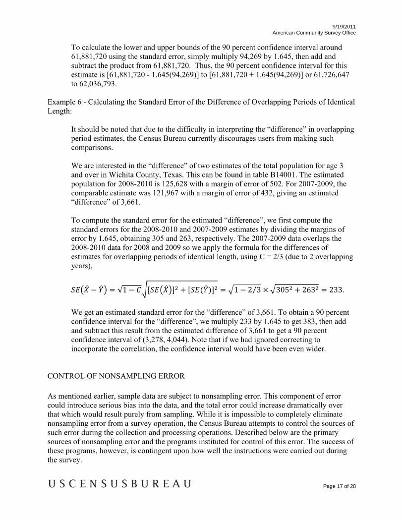
Example 6 - Calculating the Standard Error of the Difference of Overlapping Periods of Identical Length:

It should be noted that due to the difficulty in interpreting the “difference” in overlapping period estimates, the Census Bureau currently discourages users from making such comparisons. We are interested in the “difference” of two estimates of the total population for age 3 and over in Wichita County, Texas. This can be found in table B14001. The estimated population for 2008-2010 is 125,628 with a margin of error of 502. For 2007-2009, the comparable estimate was 121,967 with a margin of error of 432, giving an estimated “difference” of 3,661. To compute the standard error for the estimated “difference”, we first compute the standard errors for the 2008-2010 and 2007-2009 estimates by dividing the margins of error by 1.645, obtaining 305 and 263, respectively. The 2007-2009 data overlaps the 2008-2010 data for 2008 and 2009 so we apply the formula for the differences of estimates for overlapping periods of identical length, using C = 2/3 (due to 2 overlapping years),

√1 1 2 3⁄ 305 263 233.

We get an estimated standard error for the “difference” of 3,661. To obtain a 90 percent confidence interval for the “difference”, we multiply 233 by 1.645 to get 383, then add and subtract this result from the estimated difference of 3,661 to get a 90 percent confidence interval of (3,278, 4,044). Note that if we had ignored correcting to incorporate the correlation, the confidence interval would have been even wider.

CONTROL OF NONSAMPLING ERROR As mentioned earlier, sample data are subject to nonsampling error. This component of error could introduce serious bias into the data, and the total error could increase dramatically over that which would result purely from sampling. While it is impossible to completely eliminate nonsampling error from a survey operation, the Census Bureau attempts to control the sources of such error during the collection and processing operations. Described below are the primary sources of nonsampling error and the programs instituted for control of this error. The success of these programs, however, is contingent upon how well the instructions were carried out during the survey.


of 28

• Coverage Error — It is possible for some sample housing units or persons to be missed

entirely by the survey (undercoverage), but it is also possible for some sample housing units and persons to be counted more than once (overcoverage). Both the undercoverage and overcoverage of persons and housing units can introduce biases into the data, increase respondent burden and survey costs.

A major way to avoid coverage error in a survey is to ensure that its sampling frame, for ACS an address list in each state, is as complete and accurate as possible. The source of addresses for the ACS is the MAF, which was created by combining the Delivery Sequence File of the United States Postal Service and the address list for Census 2000. An attempt is made to assign all appropriate geographic codes to each MAF address via an automated procedure using the Census Bureau TIGER (Topologically Integrated Geographic Encoding and Referencing) files. A manual coding operation based in the appropriate regional offices is attempted for addresses, which could not be automatically coded. The MAF was used as the source of addresses for selecting sample housing units and mailing questionnaires. TIGER produced the location maps for CAPI assignments. Sometimes the MAF has an address that is the duplicate of another address already on the MAF. This could occur when there is a slight difference in the address such as 123 Main Street versus 123 Maine Street.

In the CATI and CAPI nonresponse follow-up phases, efforts were made to minimize the chances that housing units that were not part of the sample were interviewed in place of units in sample by mistake. If a CATI interviewer called a mail nonresponse case and was not able to reach the exact address, no interview was conducted and the case was eligible for CAPI. During CAPI follow-up, the interviewer had to locate the exact address for each sample housing unit. If the interviewer could not locate the exact sample unit in a multi-unit structure, or found a different number of units than expected, the interviewers were instructed to list the units in the building and follow a specific procedure to select a replacement sample unit. Person overcoverage can occur when an individual is included as a member of a housing unit but does not meet ACS residency rules. Coverage rates give a measure of undercoverage or overcoverage of persons or housing units in a given geographic area. Rates below 100 percent indicate undercoverage, while rates above 100 percent indicate overcoverage. Coverage rates are released concurrent with the release of estimates on American FactFinder in the B98 series of detailed tables. Further information about ACS coverage rates may be found at http://www.census.gov/acs/www/methodology/coverage_rates_data/.

• Nonresponse Error — Survey nonresponse is a well-known source of nonsampling error.

There are two types of nonresponse error – unit nonresponse and item nonresponse. Nonresponse errors affect survey estimates to varying levels depending on amount of nonresponse and the extent to which nonrespondents differ from respondents on the characteristics measured by the survey. The exact amount of nonresponse error or bias on an estimate is almost never known. Therefore, survey researchers generally rely on


of 28

proxy measures, such as the nonresponse rate, to indicate the potential for nonresponse error. o Unit Nonresponse — Unit nonresponse is the failure to obtain data from housing

units in the sample. Unit nonresponse may occur because households are unwilling or unable to participate, or because an interviewer is unable to make contact with a housing unit. Unit nonresponse is problematic when there are systematic or variable differences between interviewed and noninterviewed housing units on the characteristics measured by the survey. Nonresponse bias is introduced into an estimate when differences are systematic, while nonresponse error for an estimate evolves from variable differences between interviewed and noninterviewed households. The ACS makes every effort to minimize unit nonresponse, and thus, the potential for nonresponse error. First, the ACS used a combination of mail, CATI, and CAPI data collection modes to maximize response. The mail phase included a series of three to four mailings to encourage housing units to return the questionnaire. Subsequently, mail nonrespondents (for which phone numbers are available) were contacted by CATI for an interview. Finally, a subsample of the mail and telephone nonrespondents was contacted by a personal visit to attempt an interview. Combined, these three efforts resulted in a very high overall response rate for the ACS. ACS response rates measure the percent of units with a completed interview. The higher the response rate, and consequently the lower the nonresponse rate, the less chance estimates may be affected by nonresponse bias. Response and nonresponse rates, as well as rates for specific types of nonresponse, are released concurrent with the release of estimates on American FactFinder in the B98 series of detailed tables. Further information about response and nonresponse rates may be found at http://www.census.gov/acs/www/methodology/response_rates_data/.

o Item Nonresponse — Nonresponse to particular questions on the survey questionnaire and instrument allows for the introduction of error or bias into the data, since the characteristics of the nonrespondents have not been observed and may differ from those reported by respondents. As a result, any imputation procedure using respondent data may not completely reflect this difference either at the elemental level (individual person or housing unit) or on average.

Some protection against the introduction of large errors or biases is afforded by minimizing nonresponse. In the ACS, item nonresponse for the CATI and CAPI operations was minimized by the requirement that the automated instrument receive a response to each question before the next one could be asked. Questionnaires returned by mail were edited for completeness and acceptability. They were reviewed by computer for content omissions and population coverage. If necessary, a telephone follow-up was made to obtain missing information. Potential coverage errors were included in this follow-up.


of 28

Allocation tables provide the weighted estimate of persons or housing units for which a value was imputed, as well as the total estimate of persons or housing units that were eligible to answer the question. The smaller the number of imputed responses, the lower the chance that the item nonresponse is contributing a bias to the estimates. Allocation tables are released concurrent with the release of estimates on American Factfinder in the B99 series of detailed tables with the overall allocation rates across all person and housing unit characteristics in the B98 series of detailed tables. Additional information on item nonresponse and allocations can be found at http://www.census.gov/acs/www/methodology/item_allocation_rates_data/.

• Measurement and Processing Error — The person completing the questionnaire or

responding to the questions posed by an interviewer could serve as a source of error, although the questions were cognitively tested for phrasing, and detailed instructions for completing the questionnaire were provided to each household.

o Interviewer monitoring — The interviewer may misinterpret or otherwise

incorrectly enter information given by a respondent; may fail to collect some of the information for a person or household; or may collect data for households that were not designated as part of the sample. To control these problems, the work of interviewers was monitored carefully. Field staff were prepared for their tasks by using specially developed training packages that included hands-on experience in using survey materials. A sample of the households interviewed by CAPI interviewers was reinterviewed to control for the possibility that interviewers may have fabricated data.

o Processing Error — The many phases involved in processing the survey data

represent potential sources for the introduction of nonsampling error. The processing of the survey questionnaires includes the keying of data from completed questionnaires, automated clerical review, follow-up by telephone, manual coding of write-in responses, and automated data processing. The various field, coding and computer operations undergo a number of quality control checks to insure their accurate application.

o Content Editing — After data collection was completed, any remaining

incomplete or inconsistent information was imputed during the final content edit of the collected data. Imputations, or computer assignments of acceptable codes in place of unacceptable entries or blanks, were needed most often when an entry for a given item was missing or when the information reported for a person or housing unit on that item was inconsistent with other information for that same person or housing unit. As in other surveys and previous censuses, the general procedure for changing unacceptable entries was to allocate an entry for a person or housing unit that was consistent with entries for persons or housing units with similar characteristics. Imputing acceptable values in place of blanks or unacceptable entries enhances the usefulness of the data.


of 28

ISSUES WITH APPROXIMATING THE STANDARD ERROR OF LINEAR

COMBINATIONS OF MULTIPLE ESTIMATES

Several examples are provided here to demonstrate how different the approximated standard errors of sums can be compared to those derived and published with ACS microdata. These examples use estimates from the 2005-2009 ACS 5-year data products.

A. With the release of the 5-year data, detailed tables down to tract and block group will be available. At these geographic levels, many estimates may be zero. As mentioned in the ‘Calculations of Standard Errors’ section, a special procedure is used to estimate the MOE when an estimate is zero. For a given geographic level, the MOEs will be identical for zero estimates. When summing estimates which include many zero estimates, the standard error and MOE in general will become unnaturally inflated. Therefore, users are advised to sum only one of the MOEs from all of the zero estimates. Suppose we wish to estimate the total number of people whose first reported ancestry was ‘Subsaharan African’ in Rutland County, Vermont. Table A: 2005-2009 Ancestry Categories from Table B04001: First Ancestry Reported

First Ancestry Reported Category Estimate MOE Subsaharan African: 48 43 Cape Verdean 9 15 Ethiopian 0 93 Ghanian 0 93 Kenyan 0 93 Liberian 0 93 Nigerian 0 93 Senegalese 0 93 Sierra Leonean 0 93 Somalian 0 93 South African 10 16 Sudanese 0 93 Ugandan 0 93 Zimbabwean 0 93 African 20 33 Other Subsaharan African 9 16

2009 American FactFinder To estimate the total number of people, we add up all of the categories.

9 0 0 10 0 … 20 9 48


of 28

To approximate the standard error using all of the MOEs we obtiain:

15

1.64593

1.64516

1.64533

1.64516

1.645 189.3

Using only one of the MOEs from the zero estimates, we obtain:

15

1.64593

1.64516

1.64533

1.64516

1.645 62.2

From the table, we know that the actual MOE is 43, giving a standard error of 43 / 1.645 = 26.1. The first method is roughly seven times larger than the actual standard error, while the second method is roughly 2.4 times larger. Leaving out all of the MOEs from zero estimates we obtain:

15

1.64516

1.64533

1.64516

1.645 26.0

In this case, it is very close to the actual SE. This is not always the case, as can be seen in the examples below.

B. Suppose we wish to estimate the total number of males with income below the poverty level in the past 12 months using both state and PUMA level estimates for the state of Wyoming. Part of the detailed table B170012 is displayed below with estimates and their margins of error in parentheses.

2 Table C17001 is used in this example for the 2009 1-year Accuracy documents. C17001 is not published for the 2005-2009 5-year data.


of 28

Table B: 2005-2009 ACS estimates of Males with Income Below Poverty from table B17001: Poverty Status in the Past 12 Months by Sex by Age

Characteristic Wyoming PUMA 00100

PUMA 00200

PUMA 00300

PUMA 00400

Male 21,769 (1,480) 4,496 (713) 5,891 (622) 4,706 (665) 6,676 (742)

Under 5 Years 3,064 (422) 550 (236) 882 (222) 746 (196) 886 (237)

5 Years Old 348 (106) 113 (65) 89 (57) 82 (55) 64 (44)6 to 11 Years Old 2,424 (421) 737 (272) 488 (157) 562 (163) 637 (196)

12 to 14 Years Old 1,281 (282) 419 (157) 406 (141) 229 (106) 227 (111)15 Years Old 391 (128) 51 (37) 167 (101) 132 (64) 41 (38)

16 and 17 Years Old 779 (258) 309 (197) 220 (91) 112 (72) 138 (112)18 to 24 Years old 4,504 (581) 488 (192) 843 (224) 521 (343) 2,652 (481)25 to 34 Years Old 2,289 (366) 516 (231) 566 (158) 542 (178) 665 (207)35 to 44 Years Old 2,003 (311) 441 (122) 535 (160) 492 (148) 535 (169)45 to 54 Years Old 1,719 (264) 326 (131) 620 (181) 475 (136) 298 (113)55 to 64 Years Old 1,766 (323) 343 (139) 653 (180) 420 (135) 350 (125)65 to 74 Years Old 628 (142) 109 (69) 207 (77) 217 (72) 95 (55)75 Years and Older 573 (147) 94 (53) 215 (86) 176 (72) 88 (62)

2009 American FactFinder The first way is to sum the thirteen age groups for Wyoming: Estimate(Male) = 3,064 + 348 + … + 573 = 21,769. The first approximation for the standard error in this case gives us:

4221.645

1061.645 …

1471.645 696.6

A second way is to sum the four PUMA estimates for Male to obtain: Estimate(Male) = 4,496 + 5,891 + 4,706 + 6,676 = 21,769 as before. The second approximation for the standard error yields:

7131.645

6221.645

6651.645

7421.645 835.3


of 28

Finally, we can sum up all thirteen age groups for all four PUMAs to obtain an estimate based on aa total of 52 estim tes:

550 113 88 21,769

And the third approximated standard error is

4221.645

1061.645

621.645 721.9

However, we do know that the standard error using the published MOE is 1,480 /1.645 = 899.7. In this instance, all of the approximations under-estimate the published standard error and should be used with caution.

C. Suppose we wish to estimate the total number of males at the national level using age and citizenship status. The relevant data from table B05003 is displayed in table C below.

Table C: 2005-2009 ACS estimates of males from B05003: Sex by Age by Citizenship Status Characteristic Estimate MOE Male 148,535,646 6,574 Under 18 Years 37,971,739 6,285 Native 36,469,916 10,786 Foreign Born 1,501,823 11,083 Naturalized U.S. Citizen 282,744 4,284 Not a U.S. Citizen 1,219,079 10,388 18 Years and Older 110,563,907 6,908 Native 93,306,609 57,285 Foreign Born 17,257,298 52,916 Naturalized U.S. Citizen 7,114,681 20,147 Not a U.S. Citizen 10,142,617 53,041

2009 American FactFinder The estimate and its MOE are actually published. However, if they were not available in the tables, one way of obtaining them would be to add together the number of males under 18 and over 18 to get:

37,971,739 110,563,907 148,535,646 And the first approximated standard error is

148,535,6466,2851.645

6,9081.645 5,677.4


of 28

Another way would be to add up the estimates for the three subcategories (Native, and the two subcategories for Foreign Born: Naturalized U.S. Citizen, and Not a U.S. Citizen), for males

years of age. From these six estimates we obtain: under and over 18

36,469,916 282,744 1,219,079 93,306,609 7,114,681101,42,617 148,535,646

With a second approximated stan

148,535,646

10,7861.645

dard error of:

4,2841.645

10,3881.645

57,2851.645

20,1471.645

53,0411.645 49,920.0

We do know that the standard error using the published margin of error is 6,574 / 1.645 = 3,996.4. With a quick glance, we can see that the ratio of the standard error of the first method to the published-based standard error yields 1.42; an over-estimate of roughly 42%, whereas the second method yields a ratio of 12.49 or an over-estimate of 1,149%. This is an example of what could happen to the approximate SE when the sum involves a controlled estimate. In this case, it is sex by age.

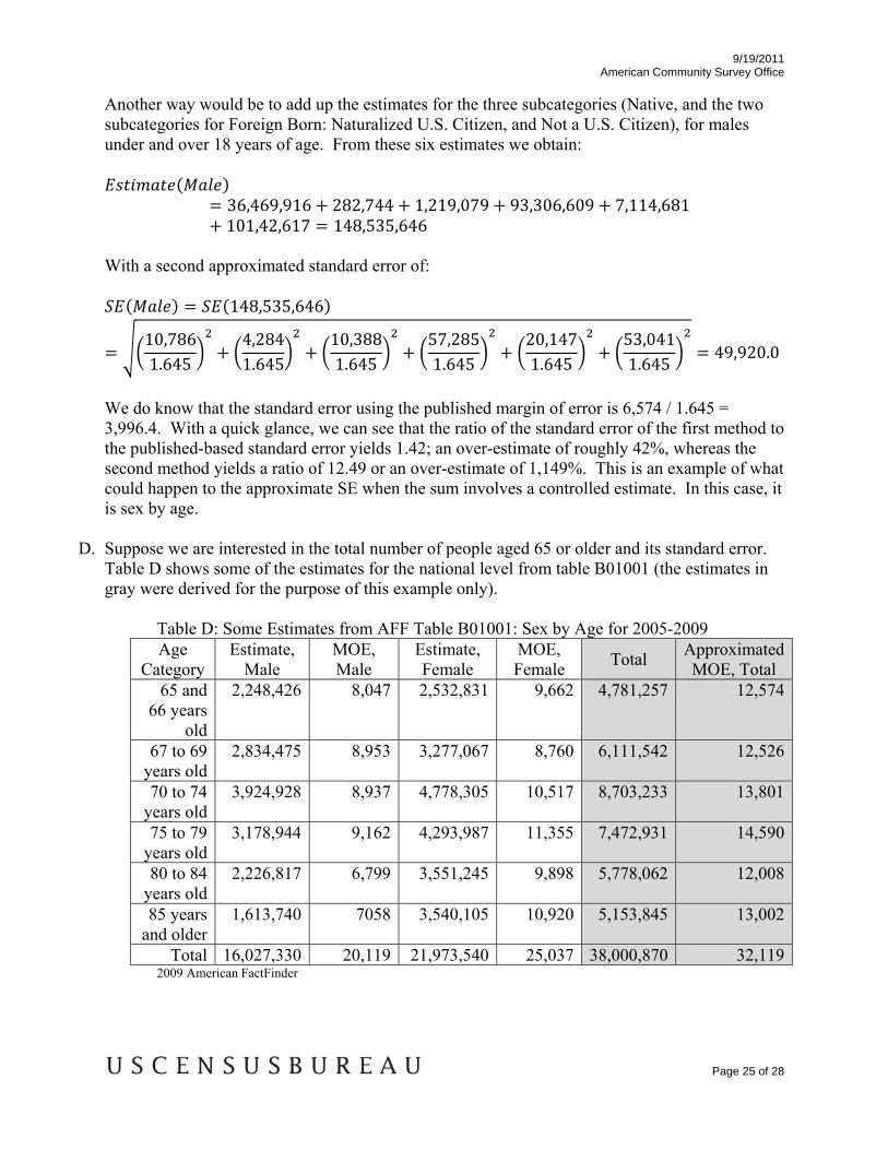
D. Suppose we are interested in the total number of people aged 65 or older and its standard error. Table D shows some of the estimates for the national level from table B01001 (the estimates in gray were derived for the purpose of this example only).

Table D: Some Estimates from AFF Table B01001: Sex by Age for 2005-2009 Age

Category Estimate,

Male MOE, Male

Estimate, Female

MOE, Female Total Approximated

MOE, Total 65 and

66 years old

2,248,426 8,047 2,532,831 9,662 4,781,257 12,574

67 to 69 years old

2,834,475 8,953 3,277,067 8,760 6,111,542 12,526

70 to 74 years old

3,924,928 8,937 4,778,305 10,517 8,703,233 13,801

75 to 79 years old

3,178,944 9,162 4,293,987 11,355 7,472,931 14,590

80 to 84 years old

2,226,817 6,799 3,551,245 9,898 5,778,062 12,008

85 years and older

1,613,740 7058 3,540,105 10,920 5,153,845 13,002

Total 16,027,330 20,119 21,973,540 25,037 38,000,870 32,1192009 American FactFinder


of 28

To begin we find the total number of people aged 65 and over by simply adding the totals for males and females to get 16,027,330 + 21,973,540 = 38,000,870. One way we could use is summing males and female for each age category and then using their MOEs to approximate the standard error for the total number of people over 65.

7 2 65 66 4,781,257 8,04 9,66 4 12,57

67 69 6,111,542 8,953 8,760 12,526 … etc. … Now, we calculate for the number of people aged 65 or older to be 38,000,870 using the six derived estimates and approximate the standard error:

38,000,870 7,6441.645

7,6141.645

8,3901.645

8,8701.645

7,3001.645

7,9041.645

32,119 For this example the estimate and its MOE are published in table B09017. The total number of people aged 65 or older is 38,000,870 with a margin of error of 4,944. Therefore the published-based standard error is:

38,000,870 4,944 1.645 3,005.⁄ The approximated standard error, using six derived age group estimates, yields an approximated standard error roughly 10.7 times larger than the published-based standard error. As a note, there are two additional ways to approximate the standard error of people aged 65 and over in addition to the way used above. The first is to find the published MOEs for the males age 65 and older and of females aged 65 and older separately and then combine to find the approximate standard error for the total. The second is to use all twelve of the published estimates together, that is, all estimates from the male age categories and female age categories, to create the SE for people aged 65 and older. However, in this particular example, the results from all three ways are the same. So no matter which way you use, you will obtain the same approximation for the SE. This is different from the results seen in example B.

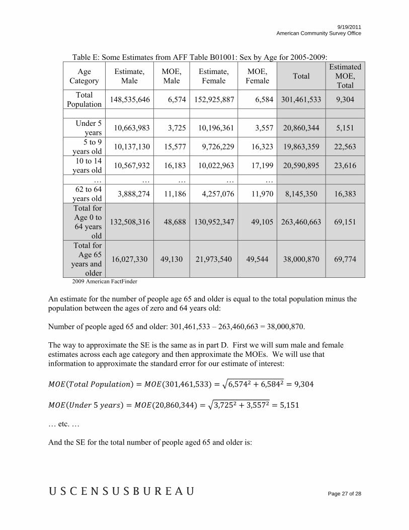
E. For an alternative to approximating the standard error for people 65 years and older seen in part D, we could find the estimate and its SE by summing all of the estimate for the ages less than 65 years old and subtracting them from the estimate for the total population. Due to the large number of estimates, Table E does not show all of the age groups. In addition, the estimates in part of the table shaded gray were derived for the purposes of this example only and cannot be found in base table B01001.


of 28

Table E: Some Estimates from AFF Table B01001: Sex by Age for 2005-2009:

Age Category

Estimate, Male

MOE, Male

Estimate, Female

MOE, Female Total

Estimated MOE, Total

Total Population 148,535,646 6,574 152,925,887 6,584 301,461,533 9,304

Under 5

years 10,663,983 3,725 10,196,361 3,557 20,860,344 5,151

5 to 9 years old 10,137,130 15,577 9,726,229 16,323 19,863,359 22,563

10 to 14 years old 10,567,932 16,183 10,022,963 17,199 20,590,895 23,616

… … … … … 62 to 64

years old 3,888,274 11,186 4,257,076 11,970 8,145,350 16,383

Total for Age 0 to 64 years

old

132,508,316 48,688 130,952,347 49,105 263,460,663 69,151

Total for Age 65

years and older

16,027,330 49,130 21,973,540 49,544 38,000,870 69,774

2009 American FactFinder An estimate for the number of people age 65 and older is equal to the total population minus the population between the ages of zero and 64 years old: Number of people aged 65 and older: 301,461,533 – 263,460,663 = 38,000,870. The way to approximate the SE is the same as in part D. First we will sum male and female estimates across each age category and then approximate the MOEs. We will use that

o t: information to approximate the standard error for our estimate f interes

301,461,533 6,574 6,584 9,304

5 20,860,344 3,725 3,557

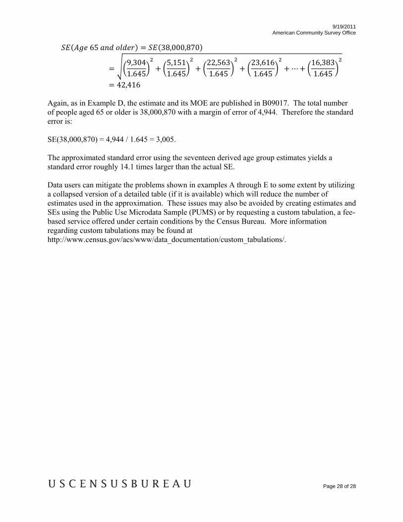
5,151 … etc. … And the SE for the total number of people aged 65 and older is:


of 28

65 38,000,870

9,3041.645

5,1511.645

22,5631.645

23,6161.645

16,3831.645

42,416 Again, as in Example D, the estimate and its MOE are published in B09017. The total number of people aged 65 or older is 38,000,870 with a margin of error of 4,944. Therefore the standard error is: SE(38,000,870) = 4,944 / 1.645 = 3,005. The approximated standard error using the seventeen derived age group estimates yields a standard error roughly 14.1 times larger than the actual SE. Data users can mitigate the problems shown in examples A through E to some extent by utilizing a collapsed version of a detailed table (if it is available) which will reduce the number of estimates used in the approximation. These issues may also be avoided by creating estimates and SEs using the Public Use Microdata Sample (PUMS) or by requesting a custom tabulation, a fee-based service offered under certain conditions by the Census Bureau. More information regarding custom tabulations may be found at http://www.census.gov/acs/www/data_documentation/custom_tabulations/.

american community survey multiyear accuracy of the … · american community survey office page 1...

Documents