an abstract of a thesis - ttu cae networkchriswilson/theses/quillen_ms.pdf · an abstract of a...
TRANSCRIPT

AN ABSTRACT OF A THESIS
J-INTEGRAL FINITE ELEMENT ANALYSISOF SEMI-ELLIPTICAL SURFACE
CRACKS IN FLAT PLATESWITH TENSILE
LOADING
Eric N. Quillen
Master of Science in Mechanical Engineering
Linear elastic fracture mechanics (LEFM) is used when response to the loadis elastic, and the fracture is brittle. For LEFM, the K-factor is the most commonlyused fracture criterion. However, high temperatures and limited high stress cycles be-fore component replacement are factors that can cause significant plastic deformationand a ductile failure. In these cases, an elastic-plastic fracture mechanics (EPFM)approach is required. The J-integral is commonly used as an EPFM fracture param-eter.
The primary goal of this research was to develop three-dimensional finite el-ement analysis (FEA) J-integral data for surface crack specimen geometries andcompare to existing solutions. The finite element models were analyzed as elas-tic, and fully plastic using ABAQUS. The J-integral data were used to find the loadindependent variable, h1 for comparison purposes.
There were two other goals in this research. The second goal was to examinethe effect of various finite element modelling parameters including mesh density, ele-ment type, symmetry, and specimen size effects, on the resulting J-integral. The thirdgoal was to perform elastic-plastic finite element analyses that utilize a stress vs. plas-tic strain table based on a power law hardening material behavior. The elastic-plasticand fully plastic results were compared.
For the most part, the current data compared well with the data published byother researchers. The elastic results compared more favorably than the fully plasticand elastic-plastic data. For both the elastic and plastic analyses, the finite elementmodels (FEMs) produced sudden increases in the K-factor and J-integral at the freesurface and/or depth. The plastic FEMs also exhibited an anomaly in the J-integralat the third and fourth angles from the surface. The anomaly could be taken as ajump at the third angle or a dip at the fourth angle, depending on how the data weretrended. The third angle varied with the model geometry (2.71◦ to 11.24◦).

J-INTEGRAL FINITE ELEMENT ANALYSIS
OF SEMI-ELLIPTICAL SURFACE
CRACKS IN FLAT PLATES
WITH TENSILE
LOADING
A Thesis
Presented to
the Faculty of the Graduate School
Tennessee Technological University
by
Eric N. Quillen
In Partial Fulfillment
of the Requirements for the Degree
MASTER OF SCIENCE
Mechanical Engineering
May 2005

STATEMENT OF PERMISSION TO USE
In presenting this thesis in partial fulfillment of the requirements for a Master
of Science degree at Tennessee Technological University, I agree that the University
Library shall make it available to borrowers under rules of the Library. Brief quota-
tions from this thesis are allowable without special permission, provided that accurate
acknowledgment of the source is made.
Permission for extensive quotation from or reproduction of this thesis may be
granted by my major professor when the proposed use of the material is for scholarly
purposes. Any copying or use of the material in this thesis for financial gain shall not
be allowed without my written permission.
Signature
Date
iii

DEDICATION
This thesis is dedicated to my wife Julie, whose encouragement has been critical
in the completion of my graduate degree and the composition of this thesis.
iv

ACKNOWLEDGMENTS
I would like to thank the following people for their help with this work: Dr.
Chris Wilson, Dr. Phillip Allen, Mike Renfro, Krishna Natarajan, and Richard
Gregory. I would also like to thank my employer, Fleetguard, Inc., and cowork-
ers. Without their cooperation, it would not have been possible for me to perform
this research.
v

TABLE OF CONTENTS
Page
LIST OF TABLES . . . . . . . . . . . . . . . . . . . . . . . . . . . . . . . . . ix
LIST OF FIGURES . . . . . . . . . . . . . . . . . . . . . . . . . . . . . . . . xiii
LIST OF SYMBOLS . . . . . . . . . . . . . . . . . . . . . . . . . . . . . . . xx
Chapter
1. INTRODUCTION . . . . . . . . . . . . . . . . . . . . . . . . . . . . . 1
1.1 Fracture Mechanics . . . . . . . . . . . . . . . . . . . . . . . 1
1.2 Overview of Research . . . . . . . . . . . . . . . . . . . . . . 2
2. TECHNICAL BACKGROUND . . . . . . . . . . . . . . . . . . . . . . 4
2.1 J-Integral . . . . . . . . . . . . . . . . . . . . . . . . . . . . 4
2.2 EPRI Estimation Scheme . . . . . . . . . . . . . . . . . . . . 8
2.3 Reference Stress Method . . . . . . . . . . . . . . . . . . . . 17
3. RESEARCH PROCEDURE . . . . . . . . . . . . . . . . . . . . . . . . 19
3.1 Finite Element Modeling . . . . . . . . . . . . . . . . . . . . 19
3.1.1 Mesh Generation . . . . . . . . . . . . . . . . . . . . . . 21
3.1.1.1 mesh3d scp . . . . . . . . . . . . . . . . . . . . . . . 21
3.1.1.2 FEA-Crack . . . . . . . . . . . . . . . . . . . . . . . 22
3.2 Analysis Procedure . . . . . . . . . . . . . . . . . . . . . . . 24
3.3 J-Integral Convergence . . . . . . . . . . . . . . . . . . . . . 26
vi

vii
Chapter Page
3.3.1 Load . . . . . . . . . . . . . . . . . . . . . . . . . . . . . 26
3.3.2 Fully Plastic Zone . . . . . . . . . . . . . . . . . . . . . 27
3.4 Comparison to Other Work . . . . . . . . . . . . . . . . . . . 31
3.4.1 Kirk and Dodds . . . . . . . . . . . . . . . . . . . . . . . 31
3.4.2 McClung et al. [15] . . . . . . . . . . . . . . . . . . . . . 35
3.4.3 Lei [17] . . . . . . . . . . . . . . . . . . . . . . . . . . . 37
3.4.4 Nasgro Computer Program . . . . . . . . . . . . . . . . 38
3.5 Mesh Refinement . . . . . . . . . . . . . . . . . . . . . . . . 40
3.6 Finite Size Effects . . . . . . . . . . . . . . . . . . . . . . . . 40
3.7 Material Properties . . . . . . . . . . . . . . . . . . . . . . . 41
3.7.1 Deformation Plasticity . . . . . . . . . . . . . . . . . . . 41
3.7.2 Incremental Plasticity . . . . . . . . . . . . . . . . . . . 43
4. RESULTS . . . . . . . . . . . . . . . . . . . . . . . . . . . . . . . . . . 49
4.1 Fully Plastic Zone . . . . . . . . . . . . . . . . . . . . . . . . 49
4.2 Kirk and Dodds Incremental Plasticity . . . . . . . . . . . . 49
4.3 McClung and Lei Comparisons . . . . . . . . . . . . . . . . . 50
4.3.1 Elastic Analysis . . . . . . . . . . . . . . . . . . . . . . . 51
4.3.2 Fully Plastic Analysis . . . . . . . . . . . . . . . . . . . 67
4.3.3 Incremental Elastic-Plastic Analysis . . . . . . . . . . . . 86
4.4 Mesh Refinement . . . . . . . . . . . . . . . . . . . . . . . . 91
4.5 Size Effects . . . . . . . . . . . . . . . . . . . . . . . . . . . 93

viii
Chapter Page
4.5.1 Height Effects . . . . . . . . . . . . . . . . . . . . . . . . 93
4.5.2 Width Effects . . . . . . . . . . . . . . . . . . . . . . . . 95
5. CONCLUSIONS AND RECOMMENDATIONS . . . . . . . . . . . . . 104
5.1 Conclusions . . . . . . . . . . . . . . . . . . . . . . . . . . . 104
5.2 Recommendations . . . . . . . . . . . . . . . . . . . . . . . . 106
REFERENCES . . . . . . . . . . . . . . . . . . . . . . . . . . . . . . . . . . 108
APPENDICES
A: INSTRUCTIONS FOR MESH3D SCP MODIFICATIONS . . . . . . . . . 113
B: COARSE VERSUS REFINED MESHES FOR K-FACTORS . . . . . . . 115
C: COARSE VS. REFINED MESHES FOR FULLY PLASTIC MODELS . . 120
D: HEIGHT EFFECTS . . . . . . . . . . . . . . . . . . . . . . . . . . . . . . 133
E: K-FACTOR RESULTS FOR COARSE MESHES . . . . . . . . . . . . . . 137
F: FULLY PLASTIC RESULTS FOR COARSE MESHES . . . . . . . . . . . 152
G: INCREMENTAL PLASTICITY TABLES . . . . . . . . . . . . . . . . . . 163
VITA . . . . . . . . . . . . . . . . . . . . . . . . . . . . . . . . . . . . . . . . 170

LIST OF TABLES
Table Page
2.1 McClung et al. h1 values in tension, n = 15 [15] . . . . . . . . . . . . . 14
2.2 McClung et al. h1 values in tension, n = 10 [15] . . . . . . . . . . . . . 14
2.3 McClung et al. h1 values in tension, n = 5 [15] . . . . . . . . . . . . . . 15
2.4 Lei h1 values in tension, n = 5 [17] . . . . . . . . . . . . . . . . . . . . 16
2.5 Lei h1 values in tension, n = 10 [17] . . . . . . . . . . . . . . . . . . . . 16
3.1 Number of nodes and elements in the duplication of the Kirk and Dodds[23] geometries . . . . . . . . . . . . . . . . . . . . . . . . . . . . . . 31
3.2 Incremental plasticity values for the Kirk and Dodds models . . . . . . 33
3.3 McClung et al. fully plastic geometries . . . . . . . . . . . . . . . . . . 36
3.4 Geometries for Nasgro comparison and width effect investigation . . . . 39
3.5 Number of crack front nodes in the coarse and refined meshes . . . . . 40
3.6 Stress vs. plastic strain data at n = 15, used for ABAQUS models . . . 47
3.7 Stress vs. plastic strain data at n = 10, used for ABAQUS models . . . 47
3.8 Stress vs. plastic strain data at n = 5, used for ABAQUS models . . . 48
4.1 Comparison of FEM results to Kirk and Dodds values . . . . . . . . . . 50
4.2 Surface and depth phenomenon for K-factors . . . . . . . . . . . . . . 56
4.3 Maximum percent differences between Newman-Raju and FEM solutions(quarter symmetry) . . . . . . . . . . . . . . . . . . . . . . . . . . . . 57
4.4 Maximum percent differences between McClung et al. [15] and FEMsolutions (quarter symmetry) . . . . . . . . . . . . . . . . . . . . . . 82
ix
x
Table Page
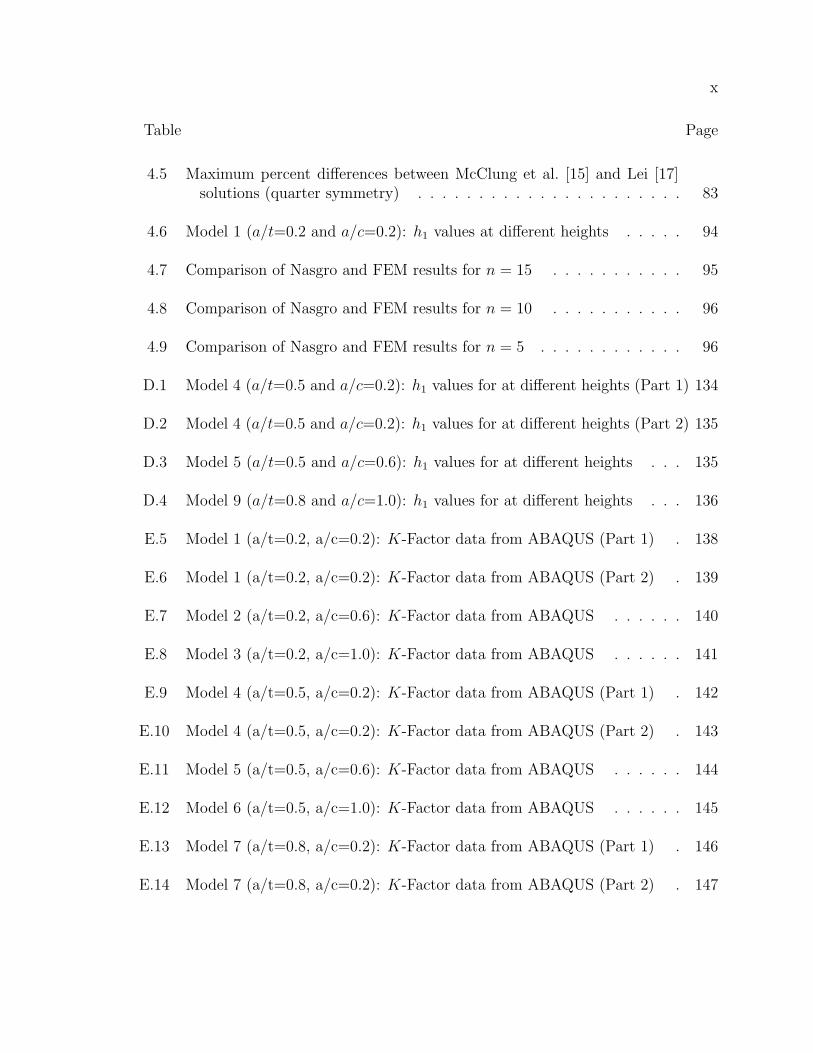
4.5 Maximum percent differences between McClung et al. [15] and Lei [17]solutions (quarter symmetry) . . . . . . . . . . . . . . . . . . . . . . 83
4.6 Model 1 (a/t=0.2 and a/c=0.2): h1 values at different heights . . . . . 94
4.7 Comparison of Nasgro and FEM results for n = 15 . . . . . . . . . . . 95
4.8 Comparison of Nasgro and FEM results for n = 10 . . . . . . . . . . . 96
4.9 Comparison of Nasgro and FEM results for n = 5 . . . . . . . . . . . . 96
D.1 Model 4 (a/t=0.5 and a/c=0.2): h1 values for at different heights (Part 1) 134
D.2 Model 4 (a/t=0.5 and a/c=0.2): h1 values for at different heights (Part 2) 135
D.3 Model 5 (a/t=0.5 and a/c=0.6): h1 values for at different heights . . . 135
D.4 Model 9 (a/t=0.8 and a/c=1.0): h1 values for at different heights . . . 136
E.5 Model 1 (a/t=0.2, a/c=0.2): K-Factor data from ABAQUS (Part 1) . 138
E.6 Model 1 (a/t=0.2, a/c=0.2): K-Factor data from ABAQUS (Part 2) . 139
E.7 Model 2 (a/t=0.2, a/c=0.6): K-Factor data from ABAQUS . . . . . . 140
E.8 Model 3 (a/t=0.2, a/c=1.0): K-Factor data from ABAQUS . . . . . . 141
E.9 Model 4 (a/t=0.5, a/c=0.2): K-Factor data from ABAQUS (Part 1) . 142
E.10 Model 4 (a/t=0.5, a/c=0.2): K-Factor data from ABAQUS (Part 2) . 143
E.11 Model 5 (a/t=0.5, a/c=0.6): K-Factor data from ABAQUS . . . . . . 144
E.12 Model 6 (a/t=0.5, a/c=1.0): K-Factor data from ABAQUS . . . . . . 145
E.13 Model 7 (a/t=0.8, a/c=0.2): K-Factor data from ABAQUS (Part 1) . 146
E.14 Model 7 (a/t=0.8, a/c=0.2): K-Factor data from ABAQUS (Part 2) . 147

xi
Table Page
E.15 Model 7 (a/t=0.8, a/c=0.2): K-Factor data from ABAQUS (Part 3) . 148
E.16 Model 8 (a/t=0.8, a/c=0.6): K-Factor data from ABAQUS (Part 1) . 149
E.17 Model 8 (a/t=0.8, a/c=0.6): K-Factor data from ABAQUS (Part 2) . 150
E.18 Model 9 (a/t=0.8, a/c=1.0): K-Factor data from ABAQUS . . . . . . 151
F.19 Model 1 (a/t=0.2, a/c=0.2): h1 data from ABAQUS . . . . . . . . . . 153
F.20 Model 2 (a/t=0.2, a/c=0.6): h1 data from ABAQUS . . . . . . . . . . 154
F.21 Model 3 (a/t=0.2, a/c=1.0): h1 data from ABAQUS . . . . . . . . . . 155
F.22 Model 4 (a/t=0.5, a/c=0.2): h1 data from ABAQUS (Part 1) . . . . . 156
F.23 Model 4 (a/t=0.5, a/c=0.2): h1 data from ABAQUS (Part 2) . . . . . 157
F.24 Model 5 (a/t=0.5, a/c=0.6): h1 data from ABAQUS . . . . . . . . . . 157
F.25 Model 6 (a/t=0.5, a/c=1.0): h1 data from ABAQUS . . . . . . . . . . 158
F.26 Model 7 (a/t=0.8, a/c=0.2): h1 data from ABAQUS (Part 1) . . . . . 159
F.27 Model 7 (a/t=0.8, a/c=0.2): h1 data from ABAQUS (Part 2) . . . . . 160
F.28 Model 8 (a/t=0.8, a/c=0.6): h1 data from ABAQUS . . . . . . . . . . 161
F.29 Model 9 (a/t=0.8, a/c=1.0): h1 data from ABAQUS . . . . . . . . . . 162
G.30 Stress vs. strain data at n = 15, based on Equation 3.13 . . . . . . . . 164
G.31 Stress vs. strain data at n = 10, based on Equation 3.13 . . . . . . . . 165
G.32 Stress vs. strain data at n = 5, based on Equation 3.13 . . . . . . . . . 166
G.33 Stress vs. plastic strain data at n = 15, used for ABAQUS models . . . 167
G.34 Stress vs. plastic strain data at n = 10, used for ABAQUS models . . . 168

xii
Table Page
G.35 Stress vs. plastic strain data at n = 5, used for ABAQUS models . . . 169

LIST OF FIGURES
Figure Page
2.1 Contour around a crack tip [4] . . . . . . . . . . . . . . . . . . . . . . . 5
2.2 EPRI J-Integral estimation scheme [4] . . . . . . . . . . . . . . . . . . 9
2.3 Sample of finite element mesh used by McClung et al. [15] . . . . . . . 12
2.4 Close up of the finite element mesh around the crack front used byMcClung et al. [15] . . . . . . . . . . . . . . . . . . . . . . . . . . . 12
3.1 Degeneration of elements around crack tip [4] . . . . . . . . . . . . . . 20
3.2 Plastic singularity element [4] . . . . . . . . . . . . . . . . . . . . . . . 20
3.3 Zones created in the mesh by mesh3d scp [20] . . . . . . . . . . . . . . 22
3.4 Mesh created using FEA-Crack . . . . . . . . . . . . . . . . . . . . . . 23
3.5 Close up of mesh from Figure 3.4 created using FEA-Crack . . . . . . . 23
3.6 Contours (semi-circular rings) around the crack tip . . . . . . . . . . . 24
3.7 Coordinate scheme for mapping crack face angles . . . . . . . . . . . . 26
3.8 Fully plastic element set consisting of the elements around the crack tip 28
3.9 Fully plastic element set consisting of part of layer 1 . . . . . . . . . . . 29
3.10 Fully plastic element set consisting of layer 1 . . . . . . . . . . . . . . . 29
3.11 Fully plastic element set consisting of partial layers 1 and 2 . . . . . . . 30
3.12 Geometries used by Kirk and Dodds for estimating the J-Integral [23] . 32
3.13 Stress vs. strain curve for Kirk and Dodds elastic-plastic models [23] . . 34
3.14 Refined mesh along the crack front . . . . . . . . . . . . . . . . . . . . 41
xiii

xiv
Figure Page
3.15 Effect of n on the stress vs. strain curve using a Ramberg-Osgood model 42
3.16 Intersection of Ramberg-Osgood curves at σo . . . . . . . . . . . . . . . 44
3.17 Elastic, modified elastic, and Ramberg-Osgood stress vs. strain curves forn = 10 . . . . . . . . . . . . . . . . . . . . . . . . . . . . . . . . . . . 45
4.1 Model 1 (a/t=0.2, a/c=0.2): Normalized K factor vs. angle along crackfront . . . . . . . . . . . . . . . . . . . . . . . . . . . . . . . . . . . . 51
4.2 Model 2 (a/t=0.2, a/c=0.6): Normalized K factor vs. angle along crackfront . . . . . . . . . . . . . . . . . . . . . . . . . . . . . . . . . . . . 52
4.3 Model 3 (a/t=0.2, a/c=1.0): Normalized K factor vs. angle along crackfront . . . . . . . . . . . . . . . . . . . . . . . . . . . . . . . . . . . . 52
4.4 Model 4 (a/t=0.5, a/c=0.2): Normalized K factor vs. angle along crackfront . . . . . . . . . . . . . . . . . . . . . . . . . . . . . . . . . . . . 53
4.5 Model 5 (a/t=0.5, a/c=0.6): Normalized K factor vs. angle along crackfront . . . . . . . . . . . . . . . . . . . . . . . . . . . . . . . . . . . . 53
4.6 Model 6 (a/t=0.5, a/c=1.0): Normalized K factor vs. angle along crackfront . . . . . . . . . . . . . . . . . . . . . . . . . . . . . . . . . . . . 54
4.7 Model 7 (a/t=0.8, a/c=0.2): Normalized K factor vs. angle along crackfront . . . . . . . . . . . . . . . . . . . . . . . . . . . . . . . . . . . . 54
4.8 Model 8 (a/t=0.8, a/c=0.6): Normalized K factor vs. angle along crackfront . . . . . . . . . . . . . . . . . . . . . . . . . . . . . . . . . . . . 55
4.9 Model 9 (a/t=0.8, a/c=1.0): Normalized K factor vs. angle along crackfront . . . . . . . . . . . . . . . . . . . . . . . . . . . . . . . . . . . . 55
4.10 Elastic singularity element [4] . . . . . . . . . . . . . . . . . . . . . . . 58
4.11 Model 1 (a/t=0.2, a/c=0.2): Normalized K-factor vs. angle along crackfront for untied and tied nodes . . . . . . . . . . . . . . . . . . . . . 58
xv
Figure Page
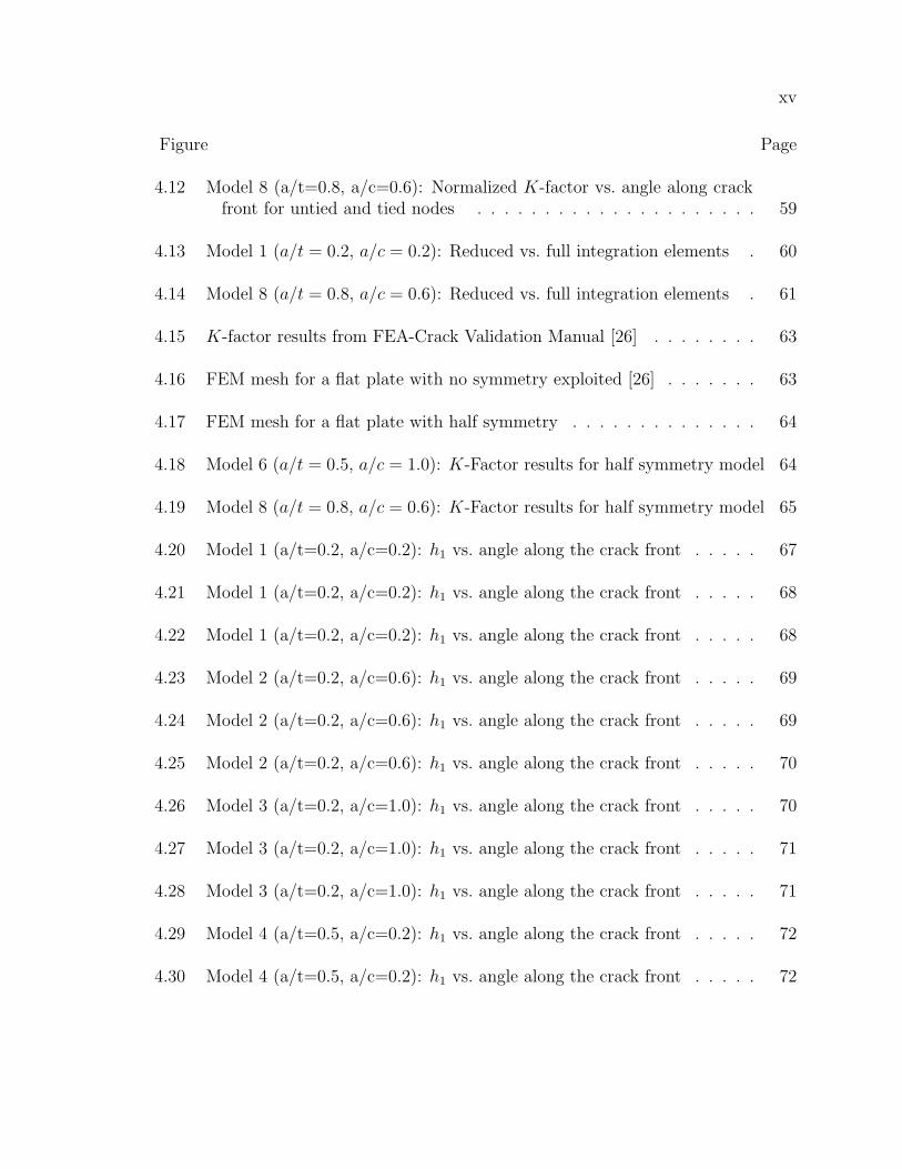
4.12 Model 8 (a/t=0.8, a/c=0.6): Normalized K-factor vs. angle along crackfront for untied and tied nodes . . . . . . . . . . . . . . . . . . . . . 59
4.13 Model 1 (a/t = 0.2, a/c = 0.2): Reduced vs. full integration elements . 60
4.14 Model 8 (a/t = 0.8, a/c = 0.6): Reduced vs. full integration elements . 61
4.15 K-factor results from FEA-Crack Validation Manual [26] . . . . . . . . 63
4.16 FEM mesh for a flat plate with no symmetry exploited [26] . . . . . . . 63
4.17 FEM mesh for a flat plate with half symmetry . . . . . . . . . . . . . . 64
4.18 Model 6 (a/t = 0.5, a/c = 1.0): K-Factor results for half symmetry model 64
4.19 Model 8 (a/t = 0.8, a/c = 0.6): K-Factor results for half symmetry model 65
4.20 Model 1 (a/t=0.2, a/c=0.2): h1 vs. angle along the crack front . . . . . 67
4.21 Model 1 (a/t=0.2, a/c=0.2): h1 vs. angle along the crack front . . . . . 68
4.22 Model 1 (a/t=0.2, a/c=0.2): h1 vs. angle along the crack front . . . . . 68
4.23 Model 2 (a/t=0.2, a/c=0.6): h1 vs. angle along the crack front . . . . . 69
4.24 Model 2 (a/t=0.2, a/c=0.6): h1 vs. angle along the crack front . . . . . 69
4.25 Model 2 (a/t=0.2, a/c=0.6): h1 vs. angle along the crack front . . . . . 70
4.26 Model 3 (a/t=0.2, a/c=1.0): h1 vs. angle along the crack front . . . . . 70
4.27 Model 3 (a/t=0.2, a/c=1.0): h1 vs. angle along the crack front . . . . . 71
4.28 Model 3 (a/t=0.2, a/c=1.0): h1 vs. angle along the crack front . . . . . 71
4.29 Model 4 (a/t=0.5, a/c=0.2): h1 vs. angle along the crack front . . . . . 72
4.30 Model 4 (a/t=0.5, a/c=0.2): h1 vs. angle along the crack front . . . . . 72

xvi
Figure Page
4.31 Model 4 (a/t=0.5, a/c=0.2): h1 vs. angle along the crack front . . . . . 73
4.32 Model 5 (a/t=0.5, a/c=0.6): h1 vs. angle along the crack front . . . . . 73
4.33 Model 5 (a/t=0.5, a/c=0.6): h1 vs. angle along the crack front . . . . . 74
4.34 Model 5 (a/t=0.5, a/c=0.6): h1 vs. angle along the crack front . . . . . 74
4.35 Model 6 (a/t=0.5, a/c=1.0): h1 vs. angle along the crack front . . . . . 75
4.36 Model 6 (a/t=0.5, a/c=1.0): h1 vs. angle along the crack front . . . . . 75
4.37 Model 6 (a/t=0.5, a/c=1.0): h1 vs. angle along the crack front . . . . . 76
4.38 Model 7 (a/t=0.8, a/c=0.2): h1 vs. angle along the crack front . . . . . 76
4.39 Model 7 (a/t=0.8, a/c=0.2): h1 vs. angle along the crack front . . . . . 77
4.40 Model 7 (a/t=0.8, a/c=0.2): h1 vs. angle along the crack front . . . . . 77
4.41 Model 8 (a/t=0.8, a/c=0.6): h1 vs. angle along the crack front . . . . . 78
4.42 Model 8 (a/t=0.8, a/c=0.6): h1 vs. angle along the crack front . . . . . 78
4.43 Model 8 (a/t=0.8, a/c=0.6): h1 vs. angle along the crack front . . . . . 79
4.44 Model 9 (a/t=0.8, a/c=1.0): h1 vs. angle along the crack front . . . . . 79
4.45 Model 9 (a/t=0.8, a/c=1.0): h1 vs. angle along the crack front . . . . . 80
4.46 Model 9 (a/t=0.8, a/c=1.0): h1 vs. angle along the crack front . . . . . 80
4.47 Model 6 (a/t=0.5, a/c=1.0): h1 results for half symmetry model at n = 15 84
4.48 Model 8 (a/t=0.8, a/c=0.6): h1 results for half symmetry model at n = 15 85
4.49 Model 1 (a/t=0.2, a/c=0.2): h1 vs. angle for fully plastic andelastic-plastic models at n=5 . . . . . . . . . . . . . . . . . . . . . . 87

xvii
Figure Page
4.50 Model 1 (a/t=0.2, a/c=0.2): h1 vs. angle for fully plastic andelastic-plastic models at n=10 . . . . . . . . . . . . . . . . . . . . . . 87
4.51 Model 1 (a/t=0.2, a/c=0.2): h1 vs. angle for fully plastic andelastic-plastic models at n=15 . . . . . . . . . . . . . . . . . . . . . . 88
4.52 Model 2 (a/t=0.2, a/c=0.6): h1 vs. angle for fully plastic andelastic-plastic models at n=5 . . . . . . . . . . . . . . . . . . . . . . 88
4.53 Model 2 (a/t=0.2, a/c=0.6): h1 vs. angle for fully plastic andelastic-plastic models at n=10 . . . . . . . . . . . . . . . . . . . . . . 89
4.54 Model 2 (a/t=0.2, a/c=0.6): h1 vs. angle for fully plastic andelastic-plastic models at n=15 . . . . . . . . . . . . . . . . . . . . . . 89
4.55 Elastic, Ramberg-Osgood, modified elastic, and modifiedRamberg-Osgood stress vs. strain curves for n = 10 . . . . . . . . . . 90
4.56 Model 1 (a/t = 0.2, a/c = 0.2): Normalized K-factor vs. angle alongcrack front . . . . . . . . . . . . . . . . . . . . . . . . . . . . . . . . . 91
4.57 Model 1 (a/t = 0.2, a/c = 0.2): h1 vs. angle along the crack front . . . 92
4.58 Model 1 (a/t = 0.2, a/c = 0.2): h1 vs. c/w for Nasgro and FEM at n = 15 97
4.59 Model 1 (a/t = 0.2, a/c = 0.2): h1 vs. c/w for Nasgro and FEM at n = 10 97
4.60 Model 1 (a/t = 0.2, a/c = 0.2): h1 vs. c/w for Nasgro and FEM at n = 5 98
4.61 Model 3 (a/t = 0.2, a/c = 1.0): h1 vs. c/w for Nasgro and FEM at n = 15 98
4.62 Model 3 (a/t = 0.2, a/c = 1.0): h1 vs. c/w for Nasgro and FEM at n = 10 99
4.63 Model 3 (a/t = 0.2, a/c = 1.0): h1 vs. c/w for Nasgro and FEM at n = 5 99
4.64 Model 4 (a/t = 0.5, a/c = 0.2): h1 vs. c/w for Nasgro and FEM at n = 15 100
4.65 Model 4 (a/t = 0.5, a/c = 0.2): h1 vs. c/w for Nasgro and FEM at n = 10 100

xviii
Figure Page
4.66 Model 4 (a/t = 0.5, a/c = 0.2): h1 vs. c/w for Nasgro and FEM at n = 5 101
4.67 Model 6 (a/t = 0.5, a/c = 1.0): h1 vs. c/w for Nasgro and FEM at n = 15 101
4.68 Model 6 (a/t = 0.5, a/c = 1.0): h1 vs. c/w for Nasgro and FEM at n = 10 102
4.69 Model 6 (a/t = 0.5, a/c = 1.0): h1 vs. c/w for Nasgro and FEM at n = 5 102
B.1 Model 1 (a/t=0.2, a/c=0.2): Normalized K factor vs. angle along crackfront . . . . . . . . . . . . . . . . . . . . . . . . . . . . . . . . . . . . 116
B.2 Model 2 (a/t=0.2, a/c=0.6): Normalized K factor vs. angle along crackfront . . . . . . . . . . . . . . . . . . . . . . . . . . . . . . . . . . . . 116
B.3 Model 3 (a/t=0.2, a/c=1.0): Normalized K factor vs. angle along crackfront . . . . . . . . . . . . . . . . . . . . . . . . . . . . . . . . . . . . 117
B.4 Model 4 (a/t=0.5, a/c=0.2): Normalized K factor vs. angle along crackfront . . . . . . . . . . . . . . . . . . . . . . . . . . . . . . . . . . . . 117
B.5 Model 5 (a/t=0.5, a/c=0.6): Normalized K factor vs. angle along crackfront . . . . . . . . . . . . . . . . . . . . . . . . . . . . . . . . . . . . 118
B.6 Model 6 (a/t=0.5, a/c=1.0): Normalized K factor vs. angle along crackfront . . . . . . . . . . . . . . . . . . . . . . . . . . . . . . . . . . . . 118
B.7 Model 8 (a/t=0.8, a/c=0.6): Normalized K factor vs. angle along crackfront . . . . . . . . . . . . . . . . . . . . . . . . . . . . . . . . . . . . 119
B.8 Model 9 (a/t=0.8, a/c=1.0): Normalized K factor vs. angle along crackfront . . . . . . . . . . . . . . . . . . . . . . . . . . . . . . . . . . . . 119
C.9 Model 1: h1 vs. angle along the crack front . . . . . . . . . . . . . . . . 121
C.10 Model 1: h1 vs. angle along the crack front . . . . . . . . . . . . . . . . 121
C.11 Model 1: h1 vs. angle along the crack front . . . . . . . . . . . . . . . . 122
C.12 Model 2: h1 vs. angle along the crack front . . . . . . . . . . . . . . . . 122

xix
Figure Page
C.13 Model 2: h1 vs. angle along the crack front . . . . . . . . . . . . . . . . 123
C.14 Model 2: h1 vs. angle along the crack front . . . . . . . . . . . . . . . . 123
C.15 Model 3: h1 vs. angle along the crack front . . . . . . . . . . . . . . . . 124
C.16 Model 3: h1 vs. angle along the crack front . . . . . . . . . . . . . . . . 124
C.17 Model 3: h1 vs. angle along the crack front . . . . . . . . . . . . . . . . 125
C.18 Model 4: h1 vs. angle along the crack front . . . . . . . . . . . . . . . . 125
C.19 Model 4: h1 vs. angle along the crack front . . . . . . . . . . . . . . . . 126
C.20 Model 4: h1 vs. angle along the crack front . . . . . . . . . . . . . . . . 126
C.21 Model 5: h1 vs. angle along the crack front . . . . . . . . . . . . . . . . 127
C.22 Model 5: h1 vs. angle along the crack front . . . . . . . . . . . . . . . . 127
C.23 Model 5: h1 vs. angle along the crack front . . . . . . . . . . . . . . . . 128
C.24 Model 6: h1 vs. angle along the crack front . . . . . . . . . . . . . . . . 128
C.25 Model 6: h1 vs. angle along the crack front . . . . . . . . . . . . . . . . 129
C.26 Model 6: h1 vs. angle along the crack front . . . . . . . . . . . . . . . . 129
C.27 Model 8: h1 vs. angle along the crack front . . . . . . . . . . . . . . . . 130
C.28 Model 8: h1 vs. angle along the crack front . . . . . . . . . . . . . . . . 130
C.29 Model 8: h1 vs. angle along the crack front . . . . . . . . . . . . . . . . 131
C.30 Model 9: h1 vs. angle along the crack front . . . . . . . . . . . . . . . . 131
C.31 Model 9: h1 vs. angle along the crack front . . . . . . . . . . . . . . . . 132
C.32 Model 9: h1 vs. angle along the crack front . . . . . . . . . . . . . . . . 132

LIST OF SYMBOLS
Symbol Description
a Crack depthaeff Effective crack length, includes plastic zoneb Uncracked ligament lengthc Half crack lengthds Increment of length along the contourG Strain energy release rateh1 Dimensionless parameter used to calculate Jpl
h2 Dimensionless parameter used to calculate CTODh3 Dimensionless parameter used to calculate δp
n Strain hardening exponentnj Unit vector components normal to Γr Crack tip radiusrc Radius of projected circlet Specimen thicknessw Half specimen widthx1 Distance along x-axis for projected circlex2 Distance along x-axis for projected circley1 Distance along y-axis for projected circley2 Distance along y-axis for projected circleA Crack areaCTOD Crack tip opening displacementE Young’s ModulusIn Integration constantJ Elastic-plastic fracture parameterJel Elastic portion of the J-integralJpl Plastic portion of the J-integralJtotal Sum of Jel and Jpl
K Stress intensity factorKnorm Normalized K-factorP Applied loadPo Limit loadTi Traction vectorui Displacement vectorW Specimen widthα Dimensionless Ramberg-Osgood material constantβ Plasticity constraint factorδp Load line displacement
xx

xxi
Symbol Description
ε Strainεij Strain tensorεo Yield strainεref Reference strainΓ ContourΠ Potential Energyµ Reference stress factorν Poisson’s ratioω Strain energy densityσ Stressσij Stress tensorσo Yield stressσref Reference stressθ Angle of crack tipEPFM Elastic plastic fracture mechanicsEPRI Electric Power Research InstituteFEA Finite element analysisFEM Finite element modelLEFM Linear elastic fracture mechanicsODB Output data base
CHAPTER 1
INTRODUCTION
1.1 Fracture Mechanics
Fracture mechanics is the study of the effects of flaws in materials under load.
Modern fracture mechanics was originated by Griffith [1] in the 1920’s when he suc-
cessfully showed that fracture in glass occurs when the strain energy resulting from
crack growth is greater than the surface energy. In 1948, Irwin [2] extended Griffith’s
strain energy release rate, G, to include metals by accounting for the energy absorbed
during plastic material flow around the flaw. By 1960, the fundamental principles of
linear elastic fracture mechanics (LEFM) were in place ([3, 4], for example).
LEFM is used to predict material failure when response to the load is elastic
and the fracture response is brittle. LEFM uses the strain energy release rate G or
the stress intensity factor K as a fracture criterion. K solutions for many geometries
have been calculated in the past and are widely available [5]. However, the design
parameters for some components violate the assumptions of LEFM. For example,
high temperatures and limited high stress cycles before component replacement are
factors that can cause significant plastic deformation and a ductile failure. In these
cases, where the LEFM approach is not valid, an elastic-plastic fracture mechanics
(EPFM) approach is required.
EPFM had its beginnings in 1961, when Wells [6] noticed that initially sharp
cracks in high toughness materials were blunted by plastic deformation. Wells pro-
posed that the distance between the crack faces at the deformed tip be used as a
1

2
measure of fracture toughness. The stretch between the crack faces at the blunted
tip is known as the crack tip opening displacement (CTOD).
In 1968 Rice [7] developed another EPFM parameter called the J-integral by
idealizing the elastic-plastic deformation around the crack tip to be nonlinear elastic.
The J-integral was shown to be equivalent to G for linear elastic deformation and to
the crack tip opening displacement for elastic-plastic deformation. During the same
year, Hutchinson [8], Rice, and Rosengren [9] showed that J was also a nonlinear
stress intensity parameter. The J-integral can be used as an elastic-plastic or fully
plastic crack growth fracture parameter, much like K is used as an elastic fracture
parameter.
The J-integral can be calculated using several experimental and analytical
techniques. The analytical techniques include the Electric Power Research Institute
(EPRI) estimation scheme, the reference stress method, and finite element methods.
It should be noted that many of the analytical techniques that do not directly require
finite element methods were established using finite element analysis.
1.2 Overview of Research
There are three goals in this research. The primary goal is to develop three-
dimensional finite element analysis (FEA) J-integral results using ABAQUS. These
results will be compared to existing solutions. The second goal is to investigate
the effect of various finite element modelling parameters on the resulting J-integral.
These parameters include mesh density, element type, symmetry, and specimen size
effects. The third goal is to compare incremental plasticity FEAs that utilize a stress
vs. plastic strain table based on a power law hardening material with the deformation
plasticity solution for a power law material. This comparison will be made in an

3
attempt to see if the fully plastic results using a deformation plasticity model can be
approached by a series of increasing loads in an incremental plasticity model.
The finite element models (FEMs) used in this research were three-dimensional
flat plates with surface cracks. The plates contained various surface crack, height, and
width geometries. Because of the dual symmetry, only one quarter of each plate was
modeled. Meshes from two different mesh generation programs were used: mesh 3d
(Faleskog, 1996) and FEA-Crack from Structural Reliability Technology.
CHAPTER 2
TECHNICAL BACKGROUND
In this chapter the J-integral and different J-integral calculation methods will
be examined. The chapter begins with a discussion of the theory and mathematical
foundation of the J-integral. Next, two methods for calculating the J-integral are
discussed: the EPRI Estimation Scheme and the reference stress method. Both of
these methods can be implemented using “hand calculations” without an extensive
fracture mechanics background. In addition, both of these methods are incorporated
into Nasgro, a fracture mechanics and fatigue crack growth program. Finally, the
FEA method is used in this research, but a review is not included here. There are
many excellent texts on the subject of FEA (for example Cook et al. [10]).
2.1 J-Integral
Rice [7] developed J as a path-independent contour integral by idealizing
elastic-plastic deformation to be the same as nonlinear elastic material behavior. In
the arbitrary path around a crack tip (Figure 2.1),
J =
∫Γ
(ωdy − Ti
∂ui
∂xds
), (2.1)
where ω is the strain energy density, Ti are components of the traction vector, ui
are the displacement vector components, and ds is an increment of length along the
4

5
Figure 2.1 Contour around a crack tip [4]
contour(Γ). The strain energy density and the traction vector components are
ω =
εij∫0
σijdεij (2.2)
and
Ti = σijnj, (2.3)
where σij is the stress tensor, εij is the strain tensor, and nj are unit vector components
normal to Γ.
In idealizing elastic-plastic behavior to be the same as nonlinear elastic material
behavior, Rice assumed that the material stress versus strain curve followed a power
law relationship. The Ramberg-Osgood equation is commonly used to describe the
stress and total strain data for this type of material response:
ε
εo
=σ
σo
+ α
(σ
σo
)n
, (2.4)

6
where ε is the total material strain, σo is the reference stress (normally defined as the
yield strength, but not necessarily the same as the 0.2% offset yield strength), εo is
the strain at the reference stress and is defined by εo = σo/E. There are two other
material constants in Equation 2.4. The first of these, α, is a dimensionless constant,
and the second, n, is the strain hardening exponent (n ≥ 1).
The J-dominated elastic-plastic stress field contains a singularity of order
r−1
n+1 . For the elastic case (n = 1), this singularity reduces to r−12 in agreement
with the K-dominated field of LEFM. The following two equations were derived by
Hutchinson [8], Rice and Rosengren [9] and are called the HRR singularity. The HRR
singularity describes the actual stresses and strains near the crack tip and within the
plastic zone as
σij = σo
(EJ
ασ2oInr
) 1n+1 ∗
σij (n, θ) (2.5)
and
εij =ασo
E
(EJ
ασ2oInr
) nn+1 ∗
εij (n, θ) , (2.6)
where In is an integration constant depending on n, r is the crack tip radius, θ is
the angle at a point around the contour, and∗
σij and∗
εij are functions of n and θ.
Equations 2.5 and 2.6 are important because the J-integral determines the stress
amplitude within the plastic zone. This fact establishes J as a fracture parameter
under conditions of plastic deformation.
7
Rice [7] also showed that the J-integral is equivalent to the energy release rate
in a nonlinear elastic material containing a crack:
J = −dΠ
dA(2.7)
where Π is the potential energy and A is the area of the crack. For linear elastic
deformation:
Jel = G =K2
E ′ (2.8)
where, for plane strain
E ′ =E
(1− ν2), (2.9)
and, for plane stress
E ′ = E. (2.10)
Care should be taken when using the energy release rate with elastic-plastic
or fully plastic deformation. In an elastic material, the potential energy is released
as the crack grows. In an elastic-plastic material, a large amount of strain energy is
used in forming a plastically deformed region around the crack tip. This energy will
not be recovered when the crack grows, or when the specimen is unloaded [4].

8
2.2 EPRI Estimation Scheme
The elastic-plastic and fully plastic J-integral estimation scheme presented by
EPRI [11] is derived from the work of Shih [12] and Hutchinson [13]. The purpose
of this work was to devise a simple handbook-style procedure for calculating the J-
integral. This goal was made possible by compiling nondimensional functions in table
form that could be used to calculate J directly. The nondimensional functions were
based on FEA results using Ramberg-Osgood materials.
The EPRI procedure computes a total J by summing the elastic and plastic
J ’s for various 2D geometries. This is expressed as
Jtotal = Jel + Jpl (2.11)
where Jtotal is the total J , Jel is the elastic portion, and Jpl is the plastic portion. For
small loads, Jel is much larger than Jpl. For large loads with significant deformation,
Jpl dominates. This situation is shown graphically in Figure 2.2. As discussed previ-
ously, elastic-plastic behavior is idealized to follow a nonlinear elastic path along the
stress versus strain curve.
In the EPRI estimation scheme, Jel is calculated utilizing an adjusted crack
length (aeff ) to compensate for the strain hardening around the crack tip and is
expressed as
Jel = G =K2(aeff )
E ′ , (2.12)

9
Figure 2.2 EPRI J-Integral estimation scheme [4]
where K is the stress intensity factor as a function of aeff . The adjusted crack length
is given by
aeff = a +1
1 + (P/Po)2
1
βπ
(n− 1
n + 1
) (KI
σo
)2
, (2.13)
where a is the half crack length, P is the applied load, Po is the limit load per unit
thickness, β = 2 for plane stress and β = 6 for plane strain, n is the strain hardening
exponent specific to the material, KI is the elastic stress intensity factor, and σo is
the reference stress (typically the yield strength).

10
The fully plastic equations for Jpl, crack mouth opening displacement (CTOD),
and load line displacement (δp), applicable for most specimen geometries are
Jpl = αεoσobh1
( a
W, n
) (P
Po
)n+1
, (2.14)
CTOD = αεoah2
( a
W, n
) (P
Po
)n
, (2.15)
and
δp = αεoah3
( a
W, n
) (P
Po
)n
, (2.16)
where α and n are a material constants, b is the uncracked ligament length, W is
the specimen width, and a is the crack length. h1, h2, and h3 are dimensionless
parameters that are a function of geometry and the hardening exponent n.
The center-cracked and single-edge-notched specimen geometries have a dif-
ferent form for Jpl. This form reduces the effect of the crack length to width ratio on
the value of h1, and is
Jpl = αεoσoba
wh1
( a
w, n
) (P
Po
)n+1
, (2.17)
where, for a center-cracked specimen, a is the half crack length and w is the half
width. Po is the reference or limit load, and is typically the load at which net cross
section yielding occurs. For center-cracked plate in tension,
Po = 4cσo
/√3 for plane strain, (2.18)

11
and
Po = 2cσo for plane stress. (2.19)
For a single-edge-crack in tension,
Po = 1.455ηcσo for plane strain, (2.20)
and
Po = 1.072ηcσo for plane stress. (2.21)
The EPRI handbook includes tabulations of h1, h2, and h3 for various n values
and geometries. These values were calculated using results from a finite element pro-
gram called INFEM [11]. INFEM was developed for the specific purpose of analyzing
fully plastic cracks and utilizes incompressible elements in the model formulation.
Further details of the finite element formulation have been published by Needleman
and Shih [14].
In 1999 McClung, Chell, Lee, and Orient [15] extended the original EPRI work
to include fully plastic J solutions for 3D geometries. This work was performed using
3D finite element models. The meshes for these models were constructed using eight-
noded brick elements in ANSYS 5.0. A typical mesh is shown in Figure 2.3. A close
up view of the crack front may be seen in Figure 2.4.

12
Figure 2.3 Sample of finite element mesh used by McClung et al. [15]
Figure 2.4 Close up of the finite element mesh around the crack front used byMcClung et al. [15]

13
Although the meshes were created in ANSYS, ABAQUS was used to perform
the analysis of the finite element models. The version of ABAQUS used for this work
was only capable of performing an incremental plasticity analysis. An EPRI-type
scheme was used to separate the elastic and plastic J values. The fully plastic values
for h1 were then calculated using
h1 =Jpl
ασoεot(
σσo
)n+1 . (2.22)
A combination of three different a/t (0.2, 0.5, 0.8) and a/c (0.2, 0.6, and 1.0)
ratios were tabulated. The specimen geometry ratios were kept constant for all models
at h/c = 4 and c/w = 0.25. The values of h1 were calculated for strain hardening
exponents of n = 5, 10, and 15, and can be found in Tables 2.1, 2.2, and 2.3.
In 2004 Lei [17] duplicated part of the work performed by McClung et al. [15]
by performing elastic and elastic-plastic finite element analyses for plates containing
semi-elliptical surface cracks under tension. The models contained surface cracks with
the same a/t and a/c ratios used by McClung et al. [15]. For the elastic analysis,
Jel results were generated and converted into K using Equation 2.8. These K results
were then compared with Newman-Raju stress-intensity factor calculations [18]. The
elastic-plastic results for strain hardening values of n = 5 and n = 10 were presented
in terms of h1. These h1 results are reproduced in Tables 2.4 and 2.5 and compare
well with McClung et al. for most geometries. The comparison with McClung et
al. and the current results are presented in more detail in Chapter 4.

14
Tab
le2.
1M
cClu
ng
etal
.h
1va
lues
inte
nsi
on,n
=15
[15]
a/t
a/c
0◦
9◦
18◦
27◦
36◦
45◦
54◦
63◦
72◦
81◦
90◦
0.20
0.20
0.22
30.
370
0.60
80.
821
1.00
11.
148
1.31
01.
447
1.56
01.
623
1.64
40.
200.
600.
356
0.46
50.
622
0.69
80.
774
0.82
30.
875
0.91
50.
948
0.97
10.
981
0.20
1.00
0.38
90.
503
0.62
80.
638
0.65
90.
653
0.65
70.
657
0.65
30.
646
0.64
60.
500.
204.
085
7.61
511
.602
14.4
8817
.057
18.7
9820
.228
21.4
3422
.129
22.2
1222
.309
0.50
0.60
3.33
64.
808
6.56
47.
048
7.69
77.
939
8.00
08.
021
8.01
97.
922
7.88
10.
501.
002.
774
3.73
84.
750
4.75
94.
932
4.89
14.
816
4.61
34.
407
4.24
34.
198
0.80
0.20
37.6
0963
.511
82.4
0491
.460
99.1
9892
.725
90.0
9788
.292
89.5
4895
.447
98.9
410.
800.
6017
.660
25.8
9032
.760
30.1
7237
.828
34.0
0231
.546
28.9
7228
.224
29.0
9530
.806
0.80
1.00
12.6
6717
.231
20.8
8219
.281
23.0
2921
.124
18.0
0516
.467
14.5
5715
.003
15.5
33
Tab
le2.
2M
cClu
ng
etal
.h
1va
lues
inte
nsi
on,n
=10
[15]
a/t
a/c
0◦
9◦
18◦
27◦
36◦
45◦
54◦
63◦
72◦
81◦
90◦
0.20
0.20
0.19
80.
320
0.52
30.
703
0.86
30.
996
1.13
31.
250
1.34
51.
398
1.41
60.
200.
600.
324
0.41
60.
544
0.60
40.
671
0.71
50.
759
0.79
20.
820
0.83
90.
847
0.20
1.00
0.35
80.
450
0.55
00.
553
0.57
10.
565
0.56
90.
566
0.56
20.
557
0.55
60.
500.
202.
539
4.51
26.
957
8.84
110
.665
11.9
7913
.048
13.9
5314
.546
14.7
1214
.811
0.50
0.60
2.31
93.
205
4.26
44.
561
4.96
75.
128
5.18
95.
209
5.23
15.
200
5.18
60.
501.
002.
007
2.59
93.
210
3.17
93.
272
3.21
83.
168
3.04
02.
921
2.82
72.
804
0.80
0.20
17.7
3129
.512
39.5
5043
.774
49.6
0046
.576
44.8
5443
.844
43.7
0645
.805
47.4
960.
800.
609.
688
13.6
8516
.725
15.8
5019
.174
17.3
1815
.896
14.7
7614
.068
14.3
2314
.800
0.80
1.00
7.24
29.
472
11.0
7710
.311
11.8
9811
.108
9.23
98.
398
7.53
67.
533
7.62
5

15
Tab
le2.
3M
cClu
ng
etal
.h
1va
lues
inte
nsi
on,n
=5
[15]
a/t
a/c
0◦
9◦
18◦
27◦
36◦
45◦
54◦
63◦
72◦
81◦
90◦
0.20
0.20
0.16
40.
252
0.40
70.
544
0.67
60.
789
0.89
70.
988
1.06
21.
103
1.11
70.
200.
600.
286
0.35
20.
441
0.48
00.
533
0.57
00.
605
0.63
10.
652
0.66
60.
672
0.20
1.00
0.32
10.
383
0.44
60.
440
0.45
20.
446
0.44
70.
442
0.43
90.
435
0.43
50.
500.
201.
325
2.13
93.
357
4.38
45.
480
6.37
17.
136
7.76
48.
222
8.42
88.
516
0.50
0.60
1.50
21.
916
2.41
22.
548
2.76
42.
860
2.91
72.
938
2.96
82.
973
2.97
60.
501.
001.
377
1.65
81.
931
1.86
71.
894
1.83
91.
800
1.73
01.
677
1.63
71.
630
0.80
0.20
7.22
411
.273
15.7
4318
.150
21.8
7021
.460
20.6
3220
.051
18.9
6018
.993
19.3
690.
800.
604.
983
6.44
97.
582
7.38
98.
421
7.75
07.
034
6.69
56.
266
6.11
46.
178
0.80
1.00
3.91
04.
728
5.25
14.
849
5.14
24.
775
4.08
03.
734
3.39
73.
285
3.27
0

16
Tab
le2.
4Lei
h1
valu
esin
tensi
on,n
=5
[17]
a/t
a/c
0◦
9◦
18◦
27◦
36◦
45◦
54◦
63◦
72◦
81◦
90◦
0.2
0.2
0.17
90.
3003
0.45
720.
5949
0.72
230.
8389
0.95
561.
053
1.13
21.
177
1.19
60.
20.
60.
3151
0.39
580.
4897
0.52
360.
5777
0.61
340.
6517
0.67
780.
7007
0.71
130.
7177
0.2
10.
3575
0.43
680.
5011
0.48
70.
5004
0.48
950.
4912
0.48
580.
4863
0.48
250.
4839
0.5
0.2
1.34
32.
327
3.49
54.
524
5.45
56.
265
7.03
97.
616
8.08
98.
338
8.46
60.
50.
61.
564
2.03
2.52
42.
633
2.82
92.
897
2.97
42.
982.
993
2.97
22.
981
0.5
11.
441.
782.
042
1.95
1.97
1.87
81.
837
1.76
21.
722
1.67
61.
672
0.8
0.2
6.72
311
.78
17.2
519
.57
21.2
21.4
321
.16
20.3
519
.57
18.9
218
.86
0.8
0.6
5.38
86.
938
8.31
78.
145
8.18
57.
656
7.17
86.
633
6.39
66.
263
6.29
0.8
14.
119
5.07
55.
678
5.18
75.
014
4.48
24.
106
3.70
13.
505
3.39
63.
406
Tab
le2.
5Lei
h1
valu
esin
tensi
on,n
=10
[17]
a/t
a/c
0◦
9◦
18◦
27◦
36◦
45◦
54◦
63◦
72◦
81◦
90◦
0.2
0.2
0.21
690.
3749
0.57
140.
7474
0.90
661.
046
1.18
61.
302
1.39
71.
451
1.47
50.
20.
60.
3554
0.45
080.
5774
0.63
30.
7033
0.75
180.
7987
0.83
380.
8627
0.87
860.
8862
0.2
10.
3995
0.50
090.
5964
0.59
950.
6222
0.61
780.
6211
0.61
90.
6193
0.61
720.
618
0.5
0.2
2.53
34.
723
6.90
78.
859
10.3
411
.45
12.4
513
.09
13.6
613
.91
14.1
10.
50.
62.
379
3.25
44.
285
4.58
84.
954
5.07
15.
164
5.14
25.
122
5.07
5.07
70.
51
2.05
52.
682
3.26
3.25
33.
341
3.23
13.
148
3.01
22.
907
2.81
82.
799
0.8
0.2
16.0
129
.51
43.2
746
.42
47.1
745
.94
45.7
145
.34
45.1
144
.93
45.3
0.8
0.6
11.0
815
.38
19.3
19.1
319
.01
17.4
316
.15
15.2
315
.31
15.4
815
.67
0.8
17.
925
10.6
812
.74
12.1
311
.77
10.4
59.
369
8.43
98.
159
8.23
8.40
8

17
2.3 Reference Stress Method
As discussed previously, the EPRI J estimation scheme assumes that the mate-
rial has a power law stress-strain curve. There are many materials that do not exhibit
this type of response. In 1984 Ainsworth [19] devised a method for calculating J that
did not depend on the material’s behavior following a power law. This approach is
called the reference stress method. The reference stress is defined as
σref =
(P
Po
)σo (2.23)
where P is the applied load, Po is the same limit load defined previously in the EPRI
research [11], and σo is the yield strength.
The reference strain, εref , is defined as the uniaxial strain corresponding to
σref . By inserting σref and εref into the Ramberg-Osgood equation 2.4, it can be
modified to the following form:
εref
εo
=σref
σo
+ α
(σref
σo
)n
. (2.24)
Using Equations 2.23 and 2.24, Equation 2.14 can be altered to the form
Jpl = σrefbh1
(εref −
σrefεo
σo
). (2.25)
Equation 2.25 still contains the variable h1, a function of n - same h1 used in the EPRI
equations discussed in the previous section. Ainsworth’s approach was to choose Po
in such a way that the dependence of h1 on n was minimized. For certain values of

18
Po, he found that h1 was relatively constant for n ≤20. As a result,
h1∼= h1
( a
w, 1
)(2.26)
where h1 is the average h1 for a range of n’s and h1
(aw, 1
)is the h1 for n equal to one.
The fully plastic solution at n = 1 is identical to the elastic solution using a Poisson’s
ratio of υ = 0.5,
µK2 (a) = bh1
( a
w, 1
)σ2
ref (2.27)
where µ=1 for plane stress and µ=0.75 for plane strain. By substituting Equation
2.27 and using the conditions that establish Equation 2.26, the Jpl expression becomes
Jpl =µKI
E
(Eεref
σref
− 1
). (2.28)
The previously discussed McClung et al. [15] finite element results were used
to develop another reference stress method. This reference stress algorithm is used
within Nasgro. Nasgro is a crack propagation and fracture mechanics program devel-
oped by NASA and the Southwest Research Institute.

CHAPTER 3
RESEARCH PROCEDURE
In this chapter, the technical approach used for this thesis is presented. The
chapter begins with a discussion of the finite element modeling including mesh gen-
eration. Next, the analysis procedure for the FEMs is discussed. Then, the work
duplicated by other researchers is reviewed, and any material properties or model
parameters specific to a geometry set are looked at as well. This duplication of other
researchers’ work was to validate the methodology used by ensuring that the J-integral
analysis could be performed properly. The chapter concludes with a discussion of the
general material properties used.
3.1 Finite Element Modeling
The finite element analysis program ABAQUS was used to calculate the K-
factors and J-integrals for a variety of specimen geometries. The models were created
with quarter symmetry to reduce the number of nodes and elements (hence, the
computational time) of each model.
Unless otherwise specified, the FEMs consisted of reduced integration, 20-
noded brick elements specified as C3D20R within ABAQUS. Reduced integration
elements are recommended in the ABAQUS User Manuals [21] for plastic and large
strain elastic models. Full integration elements tend to be overly stiff and the results
may oscillate. A reduced integration element has a softening effect on the stiffness
that improves the finite element results.
The elements around the crack tip were also of type C3D20R. However, the
elements were modified by collapsing the brick element into a wedge (Figure 3.1).
19

20
When the elements were degenerated, the mid-side nodes were not moved, and the
collapsed nodes were left untied (Figure 3.2). This allows for movement of the nodes
as the element is deformed and produces a 1/r strain singularity, which duplicates
the actual crack tip strain field in the plastic zone [4].
Figure 3.1 Degeneration of elements around crack tip [4]
Figure 3.2 Plastic singularity element [4]

21
3.1.1 Mesh Generation
Two different programs were used to generate finite element meshes. The
first, called mesh3d scp [20] by Faleskog, is available as freeware. Many early finite
element meshes in this work were generated with mesh3d scp. However, this program
has serious limitations. Therefore, a second mesh generation program, FEA-Crack,
was also used. This software is commercially available from Structural Reliability
Technology, Colorado.
3.1.1.1 mesh3d scp. The mesh generation program mesh3d scp generates
a one-quarter model of a surface cracked plate. The program assumes that both the
geometry and the load possess planes of symmetry. This program divides the model
into three zones, as shown in Figure 3.3. The element density in each zone is altered by
changing variables in the mesh3d scp input file. The node and element numbering in
each zone is controlled such that the application of boundary conditions and external
loads is simplified. The meshes used to investigate the fully plastic volume and
location were created using mesh3d scp (Figures 3.8 - 3.11).
The program mesh3d scp requires an iterative approach. The set of input
variables for the program input file are changed, the program generates a mesh, the
mesh is plotted and then examined graphically. This process is repeated until a
satisfactory mesh by appearance is created. This program is capable of generating
good meshes for some geometries. However, this program does not work well for other
specimen geometries. For these geometries, mesh3d scp was found to produce a bad
mesh, no mesh, or, in the worst cases, a mesh with errors.
This program was originally written to generate meshes for an earlier version
of ABAQUS. This makes it necessary to modify the ABAQUS input files created by

22
Figure 3.3 Zones created in the mesh by mesh3d scp [20]
mesh3d scp to make them compatible with recent releases of ABAQUS(V6.5). The
file modifications used for the models in this thesis are listed in Appendix A.
3.1.1.2 FEA-Crack. The second mesh generation program utilized for this
research is called FEA-Crack. FEA-Crack is more robust than mesh3d scp and does
not require the same iterative approach on the user’s part. The mesh density in the
area around the crack can be controlled by adjusting the program settings. Also, the
generated model may be viewed immediately, and required changes to the ABAQUS
input file are minimal. A mesh created using FEA-Crack is shown in Figures 3.4 and
3.5.

23
Figure 3.4 Mesh created using FEA-Crack
Figure 3.5 Close up of mesh from Figure 3.4 created using FEA-Crack

24
3.2 Analysis Procedure
Each FEM analyzed for this research contained 5 contours around the crack
tip, as seen in Figure 3.6. The results for the first contour are generally considered
to be less accurate than the other contours because of numerical inaccuracy [21]. For
this reason, the K-factor and J-integral data from all of the contours, except the first,
were averaged [17]. These average K-factor and J-integral were used for all further
calculations and comparisons.
The FEMs contained multiple node sets along the crack front. A node set
is a group of nodes that have been associated as a group within ABAQUS. The
number of node sets depended on the physical size of the crack front. Each of these
particular node sets contain a number of nodes with the same coordinates. In the
untied condition, one node in each node set is constrained so that it can move in only
Figure 3.6 Contours (semi-circular rings) around the crack tip

25
one or two directions (it stays on the plane of symmetry). The direction of constraint
depends on the symmetry plane. These constrained nodes are listed in another node
set called “crack front nodes,” which will be significant later. The other nodes in
each node set are not constrained.
ABAQUS generates values for the K-factor and J-integral at each of the node
sets along the crack front. An Excel macro was written to allow for examination of
the variation of the K-factor and J-integral values generated along the crack front.
The program was written to calculate the angle, as projected onto a circle, at each
crack front node. The macro first finds and records the constrained nodes found in
the node set “crack front nodes,” which is located in the ABAQUS input file. The
coordinates for each of these crack front nodes are then retrieved from the input file.
The crack coordinates are then mapped onto a circle, as shown in Figure 3.7. The
equation for the projection circle is shown below as
x22 + y2
2 = r2c . (3.1)
Two facts should be noted from Figure 3.7. First, y1 is equal to y2. Second, the
circle radius, rc, is equal to the crack depth, a. Both of the previous statements are
valid as long as a/c ≤ 1, which is the case for this research. Using this information,
Equation 3.1 can now be rearranged into the form
x2 =√
a2 − y21. (3.2)
Once x2 is known, the angle, θ, may be calculated using
θ = tan−1
(x2
y1
). (3.3)

26
Figure 3.7 Coordinate scheme for mapping crack face angles
With θ known, the variation of the K-factor and J-integral values can be mapped
along the crack front contour.
3.3 J-Integral Convergence
Two quantities were initially tested to ensure that the fully plastic FEM results
had converged. The first quantity was load. The second involved the fully plastic
zone specified for the FEMs.
3.3.1 Load
The applied load in the FEMs was adjusted until the resulting J-integral values
did not change with an increase in load. The final load step was also examined for
each model to ensure that the entire load was not applied. In cases where the entire
27
specified load was applied, the load was increased, and the FEM was analyzed again.
This ensured that the specified element set became fully plastic. The fully plastic
option in ABAQUS utilizes a Ramberg-Osgood material model and ends the analysis
when the observed strain for the selected element set exceeds the offset yield strain
by ten times, assuming the load or maximum number of increments have not been
reached. Also, to ensure sufficient steps in the model, the loads were set such that at
least 33% of the specified load was applied to the model.
3.3.2 Fully Plastic Zone
The volume and location effect of the specified fully plastic element set was
examined for two reasons. First, it was necessary to determine how much of the
specimen must become fully plastic before the J-integral converged. The second
reason was to simplify the model generation. The two mesh generation programs used
in this research, mesh3d scp and FEA-Crack, established convenient, but different,
elements sets for use as fully plastic.
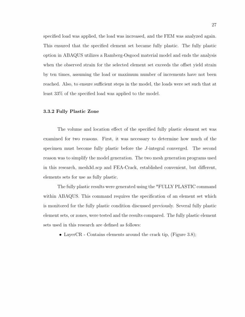
The fully plastic results were generated using the *FULLY PLASTIC command
within ABAQUS. This command requires the specification of an element set which
is monitored for the fully plastic condition discussed previously. Several fully plastic
element sets, or zones, were tested and the results compared. The fully plastic element
sets used in this research are defined as follows:
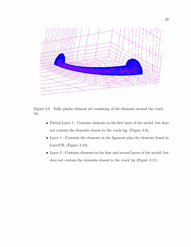
• LayerCR - Contains elements around the crack tip, (Figure 3.8);
28
Figure 3.8 Fully plastic element set consisting of the elements around the cracktip
• Partial Layer 1 - Contains elements in the first layer of the model, but does
not contain the elements closest to the crack tip, (Figure 3.9);
• Layer 1 - Contains the elements in the ligament plus the elements found in
LayerCR, (Figure 3.10);
• Layer 2 - Contains elements in the first and second layers of the model, but
does not contain the elements closest to the crack tip (Figure 3.11).

29
Figure 3.9 Fully plastic element set consisting of part of layer 1
Figure 3.10 Fully plastic element set consisting of layer 1

30
Figure 3.11 Fully plastic element set consisting of partial layers 1 and 2

31
3.4 Comparison to Other Work
A series of models with different crack ratios and specimen sizes were generated.
These models contained geometric parameters (e. g. a/t, a/c, etc.) identical to those
used by other researchers. The current results were compared to previous work with
the intent of validating the FEMs and methods used for this research.
3.4.1 Kirk and Dodds
FEMs were generated with the same geometries and material properties used
by Kirk and Dodds in 1992 [23]. These geometries are shown in Figure 3.12. The
mesh generation program mesh3d scp was used to generate models for all three cracks
defined by Kirk and Dodds. The models consisted of 20-noded brick elements with
reduced integration. The number of nodes and elements in each model is listed in
Table 3.1.
Table 3.1 Number of nodes and elements in the duplication of the Kirk and Dodds[23] geometries
Crack 1 Crack 2 Crack 3Nodes 16,597 12,227 12,227
Elements 3562 2593 2593

32
Figure 3.12 Geometries used by Kirk and Dodds for estimating the J-Integral [23]

33
These FEMs were analyzed to find Jtotal using an elastic-plastic analysis.
ABAQUS utilizes an incremental plasticity model for this type of analysis, and re-
quires a table of true stress versus plastic strain. The material properties for these
models were derived from Figure 3.13 and are listed below:
• E = 3.00× 10⁴ kpsi
• ν = 0.3
• Tangent Modulus = 3.57× 10² kpsi
• Initial Yield = 80 kpsi.
These properties were used to calculate the total and elastic strains at the yield stress
and an arbitrary stress, selected to be much higher than the applied stress. This
arbitrarily large stress was used as an input because ABAQUS does not explicitly
allow the tangent modulus to be given. The plastic strains required by ABAQUS
were found by subtracting the total and elastic strains. Table 3.2 shows the calculated
strains.
Table 3.2 Incremental plasticity values for the Kirk and Dodds models
σ, kpsi total strain elastic strain plastic strain80 2.67E-03 2.67E-03 0.00E+00200 3.36E-01 6.67E-03 3.29E-01

34
Figure 3.13 Stress vs. strain curve for Kirk and Dodds elastic-plastic models [23]

35
3.4.2 McClung et al. [15]
The mesh generation program FEA-Crack was used to generate models for all
nine geometries defined in the research performed by McClung et al. (Table 3.3). Two
sets of models were generated. The first set contained a coarse mesh. The second set
utilized a more refined mesh around the crack front. The McClung et al. geometries
were analyzed as elastic, fully plastic and incrementally plastic models. The elastic
and fully plastic analyses were performed using both the coarse and refined meshes.
The incrementally plastic models were analyzed using only the coarse meshes.
In the elastic FEM analysis, the K factor was found in two ways. First,
ABAQUS was used to calculate K directly. Second, ABAQUS was used to find
the elastic J , and then Equation 2.8 was used to calculate K. These results were
compared to K factors calculated using equations from Newman and Raju [24]. The
Newman-Raju solution is given in Equations 3.4 - 3.9.
KI = σ
√π
(a
Q
) [M1 + M2
(a
t
)2
+ M3
(a
t
)4]
gfθfw, (3.4)
Q = 1 + 1.464(a
c
)1.65
, (3.5)

36
Tab
le3.
3M
cClu
ng
etal
.fu
lly
pla
stic
geom
etries
Model1
Model2
Model3
Model4
Model5
Model6
Model7
Model8
Model9
a/t
0.2
0.2
0.2
0.5
0.5
0.5
0.8
0.8
0.8
a/c
0.2
0.6
10.
20.
61
0.2
0.6
1h/c
44
44
44
44
4c/
w0.
250.
250.
250.
250.
250.
250.
250.
250.
25t
11
11
11
11
1a
0.2
0.2
0.2
0.5
0.5
0.5
0.8
0.8
0.8
c1
0.33
0.2
2.5
0.83
0.5
41.
330.
8w
41.
330.
810
3.33
216
5.33
3.2
h4
1.33
0.8
103.
332
165.
333.
2

37
M1 = 1.13− 0.09(
ac
),
M2 = −0.54 + 0.89
0.2+(ac )
,
M3 = 0.5− 10.65+a
c+ 14
(1− a
c
)24,
(3.6)
g = 1 +
[0.1 + 0.35
(a
t
)2]
(1− sin θ)2 , (3.7)
fθ =
[(a
c
)2
cos2 θ + sin2 θ
]1/4
, (3.8)
fw =
[sec
(πc
2w
√a
t
)]1/2
, (3.9)
where KI is the K factor at a given angle, σ is the applied stress, a is the crack depth,
Q is factor applicable for ac≤ 1, c is the half crack width, t is the specimen thickness,
θ is the angle, as previously defined in Figure 3.7, along the crack front, and w is the
half specimen width.
3.4.3 Lei [17]
In 2004, Lei performed elastic and elastic-plastic J analyses on models with
the same crack geometries used by McClung et al. [15]. He also maintained a spec-
imen geometry ratio of c/w = 0.25. However, Lei deviated from the McClung et

38
al. geometries by fixing the ratio h/w at four to one instead of one to one. Lei also
fixed c, therefore fixing w and h, and varied a and t.
Lei used ABAQUS to perform the analyses on his models. He used the *CON-
TOUR INTEGRAL command within ABAQUS to generate J-integral results for
fifteen contours around the crack tip. The averages of these contours, excluding the
first, were presented. Lei found that the deviation of data from any one contour is
less than 5% of the average value.
Lei used consistent material properties in his analyses. The properties for the
elastic analyses were set at E = 500 MPa and ν = 0.3. The elastic-plastic analyses
used the Ramberg-Osgood stress-strain relationship (Equation 2.4), where σo = 1.0
MPa, α = 1, and n = 5 and 10. For all analyses, Lei used the Mises yield criterion
and small strain isotropic hardening.
3.4.4 Nasgro Computer Program
Current FEM results were compared with the results produced using the crack
propagation and fracture mechanics section of Nasgro. Nasgro is a fracture mechanics
and fatigue crack growth program developed by NASA and the Southwest Research
Institue. The same Ramberg-Osgood material properties used for the McClung ge-
ometries were duplicated for this comparison. The different geometries analyzed using
Nasgro are shown in Table 3.4.

39
Table 3.4 Geometries for Nasgro comparison and width effect investigation
Model a a/t c c/w w1 0.2 0.2 1.0 0.25 4.001a 0.2 0.2 1.0 0.50 2.001b 0.2 0.2 1.0 0.67 1.493 0.2 0.2 0.2 0.25 0.803a 0.2 0.2 0.2 0.50 0.403b 0.2 0.2 0.2 0.67 0.304 0.5 0.5 2.5 0.25 10.04a 0.5 0.5 2.5 0.33 7.584b 0.5 0.5 2.5 0.40 6.256 0.5 0.5 0.5 0.25 2.006a 0.5 0.5 0.5 0.33 1.526b 0.5 0.5 0.5 0.40 1.25

40
3.5 Mesh Refinement
Two sets of finite element models were constructed using the McClung et
al. geometries [15] found in Table 3.3. The first set contained a coarse mesh refinement
along the crack front. The coarse mesh refinement along the crack front can be seen
in Figure 3.5. The second set of models had three times more elements around the
crack front (Figure 3.14). Table 3.5 shows the number of crack front nodes in the
coarse and refined meshes.
3.6 Finite Size Effects
FEMs were generated to test the effect of specimen height and width on the
J-integral. The a/t ratios of 0.2 and 0.5, and the a/c ratios of 0.2 and 1.0 were
used in this analysis. The height effect models utilized the crack ratios for Model 1
(a/t = 0.2, a/c = 0.2), Model 4 (a/t = 0.5, a/c = 0.2), and Model 9 (a/t = 0.8, a/c =
1.0). The width effect models utilized the same model geometries used in the Nasgro
J-comparison work (Table 3.4).
Table 3.5 Number of crack front nodes in the coarse and refined meshesModel a/t a/c Coarse Refined
1 0.2 0.2 31 912 0.2 0.6 17 493 0.2 1.0 17 494 0.5 0.2 45 1335 0.5 0.6 17 496 0.5 1.0 17 497 0.8 0.2 73 2658 0.8 0.6 31 919 0.8 1.0 17 49

41
Figure 3.14 Refined mesh along the crack front
3.7 Material Properties
The material properties, unless otherwise specified, were based on a structural
steel. These are the same material properties used Natarajan [22] for some FEMs
in his thesis work involving J-integral solutions. Two different yielding models were
used in this research. The first was the Ramberg-Osgood deformation plasticity
model. The second was an incremental plasticity method requiring a table of σ and
εpl. The elastic material properties for each model depended on the yielding scheme
used for the FEA.
3.7.1 Deformation Plasticity
The following material properties were used with the *Deformation Plasticity
command in ABAQUS:

42
• E = 30.0× 10⁶ psi
• ν = 0.3
• σo = 40.0× 10³ psi
• α = 0.5
• n = 5, 10, and 15
where E is Young’s modulus, ν is Poisson’s ratio, σo is yield or reference stress, α
is a dimensionless constant as described in Equation 2.4, and n is the hardening
exponent. The effect of n on the stress vs. strain curves modelled using the Ramberg-
Osgood equation is shown in Figure 3.15. Notice that the smaller n is, the greater
the hardening slope
Figure 3.15 Effect of n on the stress vs. strain curve using a Ramberg-Osgoodmodel

43
3.7.2 Incremental Plasticity
The incremental plasticity models, with the exception of the Kirk and Dodds
comparison work, were generated using the Ramberg-Osgood equation,
ε
εo
=σ
σ0
+ α
(σ
σ0
)n
, (3.10)
shown again for convenience. The material properties listed in the previous section
were used to generate the a new Young’s modulus and a table of stress vs. plastic
strain for use in ABAQUS. The Young’s modulus, E = 30.0 × 10⁶ psi, used for the
fully plastic analyses was not used to derive the stress vs. plastic strain tables for
ABAQUS. It was replaced by a secant modulus,∗E, as shown in Equation 3.11:
∗E =
σ0
εo (1 + α). (3.11)
This value of Young’s modulus was selected because it intersects the Ramberg-Osgood
curve at the fully plastic reference stress, σo = 40.0× 10³ psi (Figure 3.16).

44
Figure 3.16 Intersection of Ramberg-Osgood curves at σo

45
Using this scheme, the elastic strain, and therefore the J-integral, will be
underestimated at low stresses (Figure 3.17). But, for sufficiently high stresses, the
elastic strain becomes overwhelmed by the plastic strain, making the error negligible.
The reference strain can now be expressed as
εo =σ0∗E
. (3.12)
Figure 3.17 Elastic, modified elastic, and Ramberg-Osgood stress vs. strain curvesfor n = 10

46
Multiplying both sides of Equation 3.10 by εo and substituting Equation 3.12 yields:
ε =σ∗E
+ αεo
(σ
σ0
)n
. (3.13)
Equation 3.13 can be divided into the elastic and plastic strains as
εel =σ∗E
, (3.14)
and
εpl = αεo
(σ
σo
)n
. (3.15)
The plastic strains at different stresses were then calculated for use with the *PLAS-
TIC command in ABAQUS for incremental plasticity analyses.
In summary, elastic-plastic material properties used in this research are based
on a modified Young’s modulus. This modification makes it possible to generate
incremental plasticity models that exhibit the same yield stress for all n’s. The elastic
properties used for the incremental plasticity analyses are∗E = 20× 106 and ν = 0.3.
The stress vs. plastic strain values used with the *Plastic command in ABAQUS are
shown in Tables 3.6 - 3.8.

47
Table 3.6 Stress vs. plastic strain data at n = 15, used for ABAQUS models
Stress Plastic Strain40000 0.00066741200 0.00103942400 0.00159843600 0.00242844800 0.00364946000 0.00542547200 0.00798248400 0.01163349600 0.01679750800 0.02404252000 0.03412453200 0.04804954400 0.06714255600 0.09313956800 0.12830258000 0.17556159200 0.2386960400 0.32252561600 0.43323162800 0.57863364000 0.76861465200 1.0156
Table 3.7 Stress vs. plastic strain data at n = 10, used for ABAQUS models
Stress Plastic Strain40000 0.044000 0.00172916248400 0.00448552800 0.01070651357200 0.02383796261600 0.05001680566000 0.09971217470400 0.19012333374800 0.34859793279200 0.61739149783600 1.060160459

48
Table 3.8 Stress vs. plastic strain data at n = 5, used for ABAQUS models
Stress Plastic Strain40000 0.044000 0.00107448400 0.00172952800 0.00267257200 0.00398661600 0.00577466000 0.00815370400 0.01125874800 0.01524579200 0.02028883600 0.02658588000 0.03435892400 0.0438596800 0.055333101200 0.069105105600 0.085493110000 0.104851114400 0.127567118800 0.15406123200 0.184783127600 0.220223132000 0.260903136400 0.307384140800 0.360265145200 0.420186149600 0.487828154000 0.563913158400 0.649209162800 0.744528167200 0.850727171600 0.968713176000 1.099441
CHAPTER 4
RESULTS
This chapter begins with a discussion of the results for various fully plastic
element sets. Next, models generated for parameters used by Kirk and Dodds [23]
are compared to published results. McClung, Lei, and Newman-Raju data are then
compared to current FEM results. Finally, the effects of the specimen size on the
J-integral are examined, and the h1 values for various specimen widths are compared
with Nasgro results.
4.1 Fully Plastic Zone
The mesh generation program mesh3d scp was used to generate FEM’s for all
four of the fully plastic zones described in Chapter 3. The same mesh was used for
each model. Only the specified fully plastic element set was changed for the different
models. It was found that the J-integral was identical for all of the described zones.
Therefore, only Partial Layer 1 was used in later fully plastic models was used for
the FEA-Crack meshes, and LayerCR was used for any fully plastic meshes produced
with mesh scp.
4.2 Kirk and Dodds Incremental Plasticity
The results for models generated per the Kirk and Dodds geometries are shown
in Table 4.1. The results compared quite well to the published data. The maximum
difference between the current results and the published data was 2.9%. It should be
noted that this excellent agreement in results was obtained even though the meshes
49

50
Table 4.1 Comparison of FEM results to Kirk and Dodds values
Crack θ◦ J (in-lb) Kirk and Dodds % Differencefrom FEM J (in-lb)
1 30.9 0.749 0.732 2.31 90 0.892 0.867 2.92 30.9 2.055 2.014 2.02 90 0.892 0.867 2.933 30.9 2.077 2.046 1.53 90 3.207 3.173 1.7
used by Kirk and Dodds contained approximately 25% the number of nodes and
elements used in this research.
4.3 McClung and Lei Comparisons
Elastic, fully plastic, and incremental plasticity FEA results for the McClung
et al. geometries are presented in this section. The elastic results are compared to the
Newman-Raju [24] calculations, and graphical trends are noted in the comparison of
Lei’s [17] elastic results. The fully plastic data are compared to the tabular data of
McClung et al. [15] and Lei [17]. The effects of mesh refinement are discussed for
both the elastic and fully plastic FEMs. Finally the incremental plasticity and fully
plastic FEA results are compared.

51
Figure 4.1 Model 1 (a/t=0.2, a/c=0.2): Normalized K factor vs. angle along crackfront
4.3.1 Elastic Analysis
The K factors obtained from the FEM’s with the McClung geometries were
normalized using
Knorm =KI
σ√
π aQ
, (4.1)
from Newman and Raju [25]. The results of the elastic FEM models and the Newman
and Raju [24] calculations are presented in Figures 4.1-4.9.

52
Figure 4.2 Model 2 (a/t=0.2, a/c=0.6): Normalized K factor vs. angle along crackfront
Figure 4.3 Model 3 (a/t=0.2, a/c=1.0): Normalized K factor vs. angle along crackfront

53
Figure 4.4 Model 4 (a/t=0.5, a/c=0.2): Normalized K factor vs. angle along crackfront
Figure 4.5 Model 5 (a/t=0.5, a/c=0.6): Normalized K factor vs. angle along crackfront
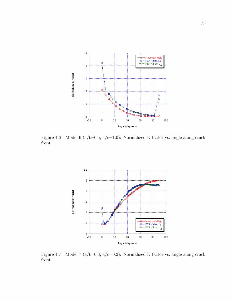
54
Figure 4.6 Model 6 (a/t=0.5, a/c=1.0): Normalized K factor vs. angle along crackfront
Figure 4.7 Model 7 (a/t=0.8, a/c=0.2): Normalized K factor vs. angle along crackfront

55
Figure 4.8 Model 8 (a/t=0.8, a/c=0.6): Normalized K factor vs. angle along crackfront
Figure 4.9 Model 9 (a/t=0.8, a/c=1.0): Normalized K factor vs. angle along crackfront

56
Significant increases in the K-factor at the surface and/or depth were observed
in all of the models. Only Models 8 (a/t = 0.8, a/c = 0.6) and 9 (a/t = 0.8, a/c = 1.0)
do not have large increases in the K-factor at the free surface. Models 1, 4, and 7
(all with a/c = 0.2) are the only FEMs that do not contain the same K-factor spike
repeated in the depth (Table 4.2).
When the surface and depth spikes are disregarded, the ABAQUS results com-
pared very reasonably to the normalized K-factors calculated per the Newman and
Raju [24] equations. This favorable comparison occurred even though the mid-side
nodes were not moved to the quarter points, and the nodes along the crack tip were
left untied (two conditions which yield optimum accuracy in K-factor calculations
using FEMs). The largest observed error, approximately six percent, occurred with
Model 8. It should also be noted that the normalized K-factor results from the K
and elastic J models were very close. The elastic results are summarized in Table
4.3. This summary disregards the surface and depth results. There is no apparent
pattern to the differences.
The current FEA results were also compared visually to the graphical results
published by Lei [17]. Lei used a different normalizing scheme, resulting in different
Table 4.2 Surface and depth phenomenon for K-factors
Surface DepthModel a/t a/c Jump Jump
1 0.2 0.2 yes no2 0.2 0.6 yes yes3 0.2 1.0 yes yes4 0.5 0.2 yes no5 0.5 0.6 yes yes6 0.5 1.0 yes yes7 0.8 0.2 yes no8 0.8 0.6 no yes9 0.8 1.0 no yes

57
Table 4.3 Maximum percent differences between Newman-Raju and FEM solu-tions (quarter symmetry)
Max FEA K Max FEA K Max FEA KDirectly from Jel from tied nodes
Model a/t a/c (% diff.) (% diff.) (% diff.)1 0.2 0.2 -5.64 -5.38 -8.52 0.2 0.6 -2.28 -2.18 -3 0.2 1.0 3.11 2.88 -4 0.5 0.2 -6.40 -5.57 -5 0.5 0.6 -2.15 -1.96 -6 0.5 1.0 3.35 3.44 -7 0.8 0.2 4.52 4.53 -8 0.8 0.6 -7.07 -7.07 -7.179 0.8 1.0 2.8 3.03 -
scales on the y-axis, but the graphs had very similar shapes. Lei also showed some
models with the same spike at the surface that was experienced in this research.
However, the increase was not as significant. No sudden increases were observed at
the depth of his elastic models.
An investigation was performed to find the cause of the previously discussed
surface and depth K-factor spikes in the current FEMs. The first step was to explore
the potential error caused by not tying the crack tip nodes or moving the mid-side
nodes to the quarter points. Model 1 (a/t = 0.2, a/c = 0.2) and Model 8 (a/t = 0.8,
a/c = 0.6) meshes were recreated in FEA-Crack for elastic analysis only. These two
models were generated with an elastic singularity, 1/√
r, created by tying the crack
tip nodes and moving the mid-side nodes to the quarter points (Figure 4.10). The
results of the two elastic models are shown graphically in Figures 4.11 and 4.12. The
K-factors produced using these two FEM’s were almost identical to the previous
results for Model 1 and Model 8.

58
Figure 4.10 Elastic singularity element [4]
Figure 4.11 Model 1 (a/t=0.2, a/c=0.2): Normalized K-factor vs. angle alongcrack front for untied and tied nodes

59
Figure 4.12 Model 8 (a/t=0.8, a/c=0.6): Normalized K-factor vs. angle alongcrack front for untied and tied nodes

60
The second step in investigating the surface and depth K-factor spikes in-
volved changing from reduced integration to full integration elements, type C3D20R
to C3D20 in ABAQUS, for the FEMs. The results for Models 1 and 8 are shown in
Figures 4.13 and 4.14. As mentioned in the ABAQUS User’s Manuals [21], using a
full integration element type caused the K-factor results to oscillate. Full integration
elements did not correct the surface and depth deviations.
Figure 4.13 Model 1 (a/t = 0.2, a/c = 0.2): Reduced vs. full integration elements

61
Figure 4.14 Model 8 (a/t = 0.8, a/c = 0.6): Reduced vs. full integration elements

62
The default nonlinear solver for ABAQUS was also considered as a possible
source of error in the third attempt to reduce the surface and depth K-factor dis-
crepencies. Since the K-factor calculation is linear, the solver used within ABAQUS
was changed to a linear perturbation. Unfortunately, the *CONTOUR INTEGRAL
command used to output the K-factors will not function within a linear perturbation
step. Another attempt to force a linear solution was made by using the *STATIC
command to force the solution to be performed in one step. The surface and depth
results were not altered by this approach.
In a fourth attempt to solve the free surface and depth spikes, the FEA-
Crack Validation Manual [26] was examined. It was found that the FEA programs
WARP3D [27], ABAQUS, and ANSYS were used to produce K-factor calculations
for validating FEA-Crack meshes. The validation data were presented graphically as
K-factor vs. angle along the crack front (Figure 4.15 [26]). The K-factors produced
by these three FEA programs were virtually identical, except at the free surface. At
this location, the K-factor produced by ABAQUS was approximately 7.7% higher
than the other two FEA programs. It was also noted that there were no irregularities
presented in the depth.
Further examination of the FEA-Crack Validation Manual [26] revealed that
the surface crack results published in the validation manual were for full plates with no
symmetry conditions (Figure 4.16). To investigate boundary conditions in the depth
phenomenon, Model 6 (a/t = 0.5, a/c = 1.0) and Model 8 (a/t = 0.8, a/c = 0.6)
meshes were created with half symmetry (Figure 4.17). The results may be seen in
Figures 4.18 and 4.19.

63
Figure 4.15 K-factor results from FEA-Crack Validation Manual [26]
Figure 4.16 FEM mesh for a flat plate with no symmetry exploited [26]

64
Step: Step-1, Stress Analysis, Step # 1Increment 9: Step Time = 0.3394
3-D crack mesh model generated by FEA-CrackODB: model6-hs.odb ABAQUS/Standard 6.2-007 Sat Dec 18 11:58:57 CST 2004
1
2
3
Step: Step-1, Stress Analysis, Step # 1Increment 9: Step Time = 0.3394
3-D crack mesh model generated by FEA-CrackODB: model6-hs.odb ABAQUS/Standard 6.2-007 Sat Dec 18 11:58:57 CST 2004
Figure 4.17 FEM mesh for a flat plate with half symmetry
Figure 4.18 Model 6 (a/t = 0.5, a/c = 1.0): K-Factor results for half symmetrymodel

65
Figure 4.19 Model 8 (a/t = 0.8, a/c = 0.6): K-Factor results for half symmetrymodel

66
The half symmetry models produced with FEA-Crack did not exhibit a K-
factor spike in the depth. Therefore, it was deduced that the boundary conditions
specified in the ABAQUS input file could be an issue. Perhaps the solver within
ABAQUS is very sensitive to the boundary conditions. Problems with the boundary
conditions in the depth or at the free surface could account for the observed increases.
An ABAQUS input file for an elastic model was examined to investigate the
boundary conditions of nodes along the crack front. For the elastic models, it was
found that there were no coincident nodes along the crack front. The crack tip nodes
were shared by the surrounding elements. The depth node was constrained in the
directions perpendicular and parallel to the crack front. All of the other crack tip
nodes were constrained only in the direction perpendicular to the crack front. This
constraint scheme is logical given a quarter symmetry model with tied nodes along
the crack front.
A possible explanation for the surface deviation is that it is a result of the
surface elements in the 3-D model. The lateral surface is subjected to plane stress,
but the surface elements have some thickness in the direction normal to the free
surface. This is a plausible, but unproven, explanation for the source of the surface
phenomenon.
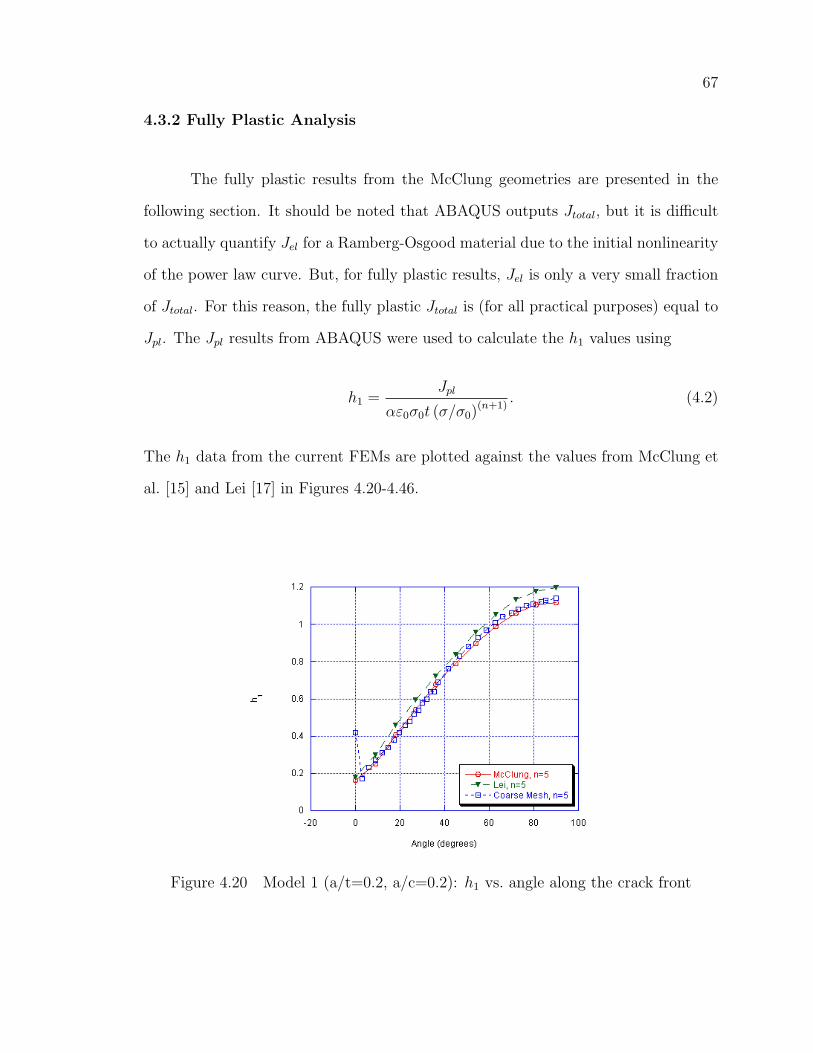
67
4.3.2 Fully Plastic Analysis
The fully plastic results from the McClung geometries are presented in the
following section. It should be noted that ABAQUS outputs Jtotal, but it is difficult
to actually quantify Jel for a Ramberg-Osgood material due to the initial nonlinearity
of the power law curve. But, for fully plastic results, Jel is only a very small fraction
of Jtotal. For this reason, the fully plastic Jtotal is (for all practical purposes) equal to
Jpl. The Jpl results from ABAQUS were used to calculate the h1 values using
h1 =Jpl
αε0σ0t (σ/σ0)(n+1)
. (4.2)
The h1 data from the current FEMs are plotted against the values from McClung et
al. [15] and Lei [17] in Figures 4.20-4.46.
Figure 4.20 Model 1 (a/t=0.2, a/c=0.2): h1 vs. angle along the crack front

68
Figure 4.21 Model 1 (a/t=0.2, a/c=0.2): h1 vs. angle along the crack front
Figure 4.22 Model 1 (a/t=0.2, a/c=0.2): h1 vs. angle along the crack front

69
Figure 4.23 Model 2 (a/t=0.2, a/c=0.6): h1 vs. angle along the crack front
Figure 4.24 Model 2 (a/t=0.2, a/c=0.6): h1 vs. angle along the crack front

70
Figure 4.25 Model 2 (a/t=0.2, a/c=0.6): h1 vs. angle along the crack front
Figure 4.26 Model 3 (a/t=0.2, a/c=1.0): h1 vs. angle along the crack front

71
Figure 4.27 Model 3 (a/t=0.2, a/c=1.0): h1 vs. angle along the crack front
Figure 4.28 Model 3 (a/t=0.2, a/c=1.0): h1 vs. angle along the crack front
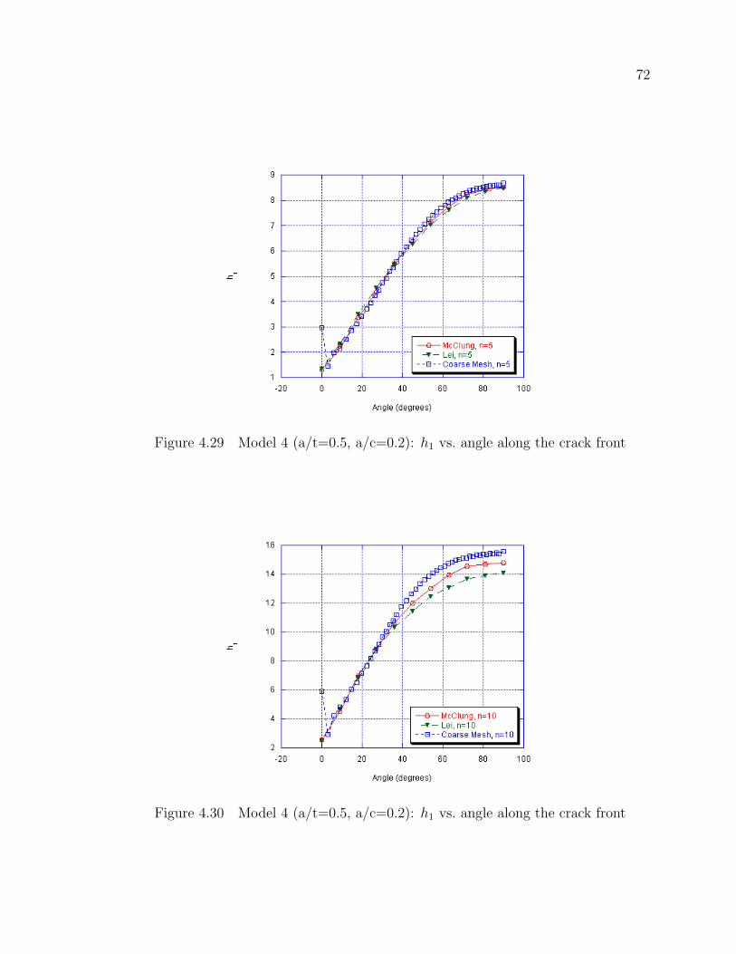
72
Figure 4.29 Model 4 (a/t=0.5, a/c=0.2): h1 vs. angle along the crack front
Figure 4.30 Model 4 (a/t=0.5, a/c=0.2): h1 vs. angle along the crack front

73
Figure 4.31 Model 4 (a/t=0.5, a/c=0.2): h1 vs. angle along the crack front
Figure 4.32 Model 5 (a/t=0.5, a/c=0.6): h1 vs. angle along the crack front

74
Figure 4.33 Model 5 (a/t=0.5, a/c=0.6): h1 vs. angle along the crack front
Figure 4.34 Model 5 (a/t=0.5, a/c=0.6): h1 vs. angle along the crack front

75
Figure 4.35 Model 6 (a/t=0.5, a/c=1.0): h1 vs. angle along the crack front
Figure 4.36 Model 6 (a/t=0.5, a/c=1.0): h1 vs. angle along the crack front

76
Figure 4.37 Model 6 (a/t=0.5, a/c=1.0): h1 vs. angle along the crack front
Figure 4.38 Model 7 (a/t=0.8, a/c=0.2): h1 vs. angle along the crack front

77
Figure 4.39 Model 7 (a/t=0.8, a/c=0.2): h1 vs. angle along the crack front
Figure 4.40 Model 7 (a/t=0.8, a/c=0.2): h1 vs. angle along the crack front

78
Figure 4.41 Model 8 (a/t=0.8, a/c=0.6): h1 vs. angle along the crack front
Figure 4.42 Model 8 (a/t=0.8, a/c=0.6): h1 vs. angle along the crack front
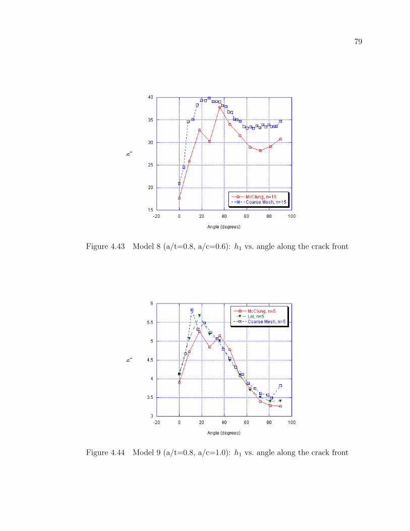
79
Figure 4.43 Model 8 (a/t=0.8, a/c=0.6): h1 vs. angle along the crack front
Figure 4.44 Model 9 (a/t=0.8, a/c=1.0): h1 vs. angle along the crack front

80
Figure 4.45 Model 9 (a/t=0.8, a/c=1.0): h1 vs. angle along the crack front
Figure 4.46 Model 9 (a/t=0.8, a/c=1.0): h1 vs. angle along the crack front

81
The same spikes observed at the free surface and in the depth of the elastic
FEMs were also found in the fully plastic models. These discrepencies matched those
found for the elastic models (Table 4.2). As seen in the elastic results, the fully plastic
models, except Models 8 (a/t = 0.8, a/c = 0.6) and 9 (a/t = 0.8, a/c = 1.0), exhibited
noticeable increases at the free surface. Models 1, 4, and 7 (all with a/c = 0.2) were
the only models that did not also contain increases in the depth.
The fully plastic results from the current FEMs, McClung, and Lei did not
correlate as well as the elastic results compared with the Newman-Raju solutions.
The differences were estimated by visually examining the previous h1 plots (Figures
4.20-4.46). The comparison was visual because the angles for McClung et al. and Lei
results did not match the angles used for this research, and a method to force the
FEA-Crack or mesh3d scp mesh generation programs to place node sets at specific
angles was not known. As with the elastic analysis, the surface and depth results
were disregarded in determining the percent differences.
A visual examination of the h1 plots revealed some interesting findings. First,
the Lei results do not contain the same spikes in the h1 values at the surface and
depth that are observed in in the current FEMs. This is intriguing because the Lei
FEA work was performed using quarter symmetry flat plates in ABAQUS.
Second, the McClung et al. and current FEM results compared reasonably well
for some crack geometries but not for others. It was found that the differences between
the two sets of results increased with n. There were differences of approximately
thirty percent for some of the n = 15 models. Table 4.4 contains the largest percent
difference between the McClung et al. and current FEM results for each model.
It was observed that Models 2, 3, 5, 6, 8, and 9 (all with a/c = 0.6 or 1.0)
of the current FEMs, exhibited either spikes in h1 at the third angle or dips at the

82
fourth angle from the surface for for all three n’s. The uncertainty of a spike at the
third angle or a dip at the fourth is due to the fact that this judgement is relative to
how the data trend is pictured. The values in Table 4.4 are highlighted with the *
symbol when the largest difference from the McClung et al. results occurred at the
third angle. The difference between results did not tend to be as significant at the
fourth angle. An examination of the FEMs for these models revealed that third angle
for each model, except Model 8, was located at 11.24◦. The third angle in Model 8
occurrs at 8.09◦. Both the McClung et al. and Lei data exhibited the same behavior.
These results occurred at an angle of 18◦.
The third observation was that Lei [17] tended to correlate more closely with
the McClung et al. [15] results than the current FEMs. Unlike the current FEMs, the
Lei models did not exhibit a consistent increase in the difference as n increased. The
maximum percent difference between the two sets of results was twenty percent, ten
percent less than the difference of the current FEA results. Table 4.5 lists the largest
percent difference between the McClung et al. and Lei results for each model.
Table 4.4 Maximum percent differences between McClung et al. [15] and FEMsolutions (quarter symmetry)
n = 5 n = 10 n = 15Model a/t a/c (% diff.) (% diff.) (% diff.)
1 0.2 0.2 2.00 -5.66 -12.502 0.2 0.6 9.20 -9.26 -12.903 0.2 1.0 12.20∗ −16.67∗ 18.52∗
4 0.5 0.2 4.67 7.69 9.095 0.5 0.6 17.5∗ 15.71∗ 21.57∗
6 0.5 1.0 15.17∗ 25.93∗ 23.17∗
7 0.8 0.2 13.33 17.78 29.358 0.8 0.6 10.81 18.75 30.009 0.8 1.0 16.00∗ 23.30∗ 28.5∗
Note: Maximum differences at the third anglefrom the surface are marked by *.
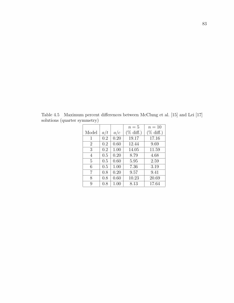
83
Table 4.5 Maximum percent differences between McClung et al. [15] and Lei [17]solutions (quarter symmetry)
n = 5 n = 10Model a/t a/c (% diff.) (% diff.)
1 0.2 0.20 19.17 17.162 0.2 0.60 12.44 9.693 0.2 1.00 14.05 11.594 0.5 0.20 8.79 4.685 0.5 0.60 5.95 2.596 0.5 1.00 7.36 3.197 0.8 0.20 9.57 9.418 0.8 0.60 10.23 20.699 0.8 1.00 8.13 17.64

84
The J-integral spikes at the free surface and depth were also investigated for
the fully plastic FEMs. As discussed in the analysis of the elastic results, the free
surface phenomenon can be attributed, at least partially, to a plane stress issue.
Fully plastic models with half symmetry were also analyzed to ensure that the depth
phenomenon disappeared under conditions of severe deformation. Model 6 (a/t = 0.5,
a/c = 1.0) and Model 8 (a/t = 0.8, a/c = 0.6) geometries were again used. The half
symmetry models did not exhibit the jump in h1 in the depth (Figures 4.47 and 4.48).
Figure 4.47 Model 6 (a/t=0.5, a/c=1.0): h1 results for half symmetry model atn = 15

85
Figure 4.48 Model 8 (a/t=0.8, a/c=0.6): h1 results for half symmetry model atn = 15
86
An ABAQUS input file for an plastic model was also examined to investigate
the boundary conditions of nodes along the crack tip. As discussed previously, the
models with untied nodes contain multiple node sets along the crack front. The nodes
at each node set along the crack tip are coincident. In the depth node set, one node
was constrained in the directions perpendicular and parallel to the crack front. The
remaining nodes in the depth were only constrained in the direction perpendicular
to the crack front. The remaining node sets, including the surface, contained one
node that was constrained in the direction perpendicular to the crack front. All other
nodes in the remaining sets were left unconstrained. This constraint scheme is logical
given a quarter symmetry model with untied nodes along the crack front.
4.3.3 Incremental Elastic-Plastic Analysis
The elastic-plastic results are compared to the fully plastic results for Model
1 (a/t=0.2, a/c=0.2) and Model 2 (a/t=0.2, a/c=0.6) for n = 5, 10, and 15. These
results are shown graphically in Figures 4.49 - 4.54.

87
Figure 4.49 Model 1 (a/t=0.2, a/c=0.2): h1 vs. angle for fully plastic and elastic-plastic models at n=5
Figure 4.50 Model 1 (a/t=0.2, a/c=0.2): h1 vs. angle for fully plastic and elastic-plastic models at n=10

88
Figure 4.51 Model 1 (a/t=0.2, a/c=0.2): h1 vs. angle for fully plastic and elastic-plastic models at n=15
Figure 4.52 Model 2 (a/t=0.2, a/c=0.6): h1 vs. angle for fully plastic and elastic-plastic models at n=5

89
Figure 4.53 Model 2 (a/t=0.2, a/c=0.6): h1 vs. angle for fully plastic and elastic-plastic models at n=10
Figure 4.54 Model 2 (a/t=0.2, a/c=0.6): h1 vs. angle for fully plastic and elastic-plastic models at n=15

90
It was found that the h1 values of the elastic-plastic method varied with the
applied stress, but appeared to converge with the fully plastic results as the stress
was increased. The similarities between the elastic-plastic and fully plastic results
included the surface, depth, and interior angle anomalies discussed previously.
Some of the differences between the elastic-plastic and fully plastic results at
lower stresses may have been due to a mistake. The wrong stress versus plastic strain
tables were used in ABAQUS. The tables actually used for the elastic-plastic analyses
in this research are located in Appendix G. These plastic strain tables contain stresses
lower than the 40 ksi yield strength discussed in Chapter 3. This caused the utilized
stress-strain curve to be lower than the Ramberg-Osgood curve at lower stresses
(Figure 4.55). However, the difference due to this error is likely small for a fully
plastic condition.
Figure 4.55 Elastic, Ramberg-Osgood, modified elastic, and modified Ramberg-Osgood stress vs. strain curves for n = 10

91
4.4 Mesh Refinement
The refined meshes made no notable difference in the normalized K factors
from the elastic analyses or the h1 values from the fully plastic analyses. A graphical
comparison of the Newman-Raju calculations, coarse mesh, and refined mesh for K-
factor analysis is shown in Figure 4.56. A graphical comparison of the McClung
results, coarse mesh, and refined mesh for the h1 analysis is shown in Figure 4.57.
The full set of results comparing the Newman-Raju calculations, the coarse meshes,
and the refined meshes are shown graphically in Appendix B. The full set of results
comparing the McClung work, the coarse meshes, and the refined meshes are shown
graphically in Appendix C.
Figure 4.56 Model 1 (a/t = 0.2, a/c = 0.2): Normalized K-factor vs. angle alongcrack front

92
Figure 4.57 Model 1 (a/t = 0.2, a/c = 0.2): h1 vs. angle along the crack front
It should be noted that the refined FEM mesh for Model 7 (a/t = 0.8, a/c =
0.2) would not run in ABAQUS. The Model 7 geometry generated the largest FEM in
this research, containing 12,140 elements and 56,142 nodes. A warning was generated
about the number of history requests for the ABAQUS output database (ODB) file,
but the terminal error was not explicitly mentioned by ABAQUS. Because the other
refined mesh models generated results that closely matched the coarse mesh models,
this exact cause of this issue was not pursued.
The same anomalies observed in the coarse mesh FEM’s were also present in
the refined mesh models. This includes the K-factor and J-integral spikes at the
free surface and depth. It should be noted that the mesh refinement did reduce the
magnitude of the surface and depth surges. The phenomenon at third and fourth
angles from the surface was also present. The values of the third and fourth angle in
the refined meshes were occurred at either 3.75◦ or 2.71◦.

93
Many of the refined mesh models contain noticeable oscillations in the h1 data
around the crack tip. This oscillation was most significant in Models 3 (a/t = 0.2,
a/c = 1.0), 4 (a/t = 0.5, a/c = 0.2), and 6 (a/t = 0.5, a/c = 1.0). For each of these
models, the magnitude of the oscillation became larger as n increased.
4.5 Size Effects
4.5.1 Height Effects
Finite element models with four different crack ratios, each at three different
heights, were analyzed to check for a height effect. Although small differences were
noticed (maximum difference of 5%), no appreciable height effect was observed. The
results for Model 1 (a/t=0.2, a/c=0.2) can be seen in Table 4.6. The results for
Models 4 (a/t=0.5, a/c=0.2), 5 (a/t=0.2, a/c=0.6), and 9 (a/t=0.8, a/c=1.0) may
be found in Appendix D.

94
Table 4.6 Model 1 (a/t=0.2 and a/c=0.2): h1 values at different heights
θ h/w = 1 h/w = 3 h/w = 50.00 0.51 0.51 0.513.04 0.20 0.20 0.206.10 0.28 0.28 0.289.00 0.34 0.33 0.3311.93 0.39 0.39 0.3814.60 0.44 0.44 0.4417.30 0.49 0.48 0.4819.73 0.54 0.53 0.5322.19 0.58 0.58 0.5824.25 0.61 0.61 0.6126.35 0.67 0.66 0.6628.23 0.69 0.68 0.6830.15 0.75 0.74 0.7431.88 0.76 0.76 0.7633.64 0.84 0.83 0.8335.24 0.83 0.82 0.8236.87 0.89 0.88 0.8841.60 1.00 0.99 0.9946.71 1.08 1.07 1.0750.74 1.16 1.14 1.1555.15 1.23 1.21 1.2158.76 1.28 1.26 1.2762.80 1.33 1.31 1.3166.12 1.37 1.35 1.3569.95 1.40 1.39 1.3973.03 1.43 1.41 1.4176.79 1.45 1.43 1.4479.57 1.47 1.45 1.4583.44 1.48 1.46 1.4685.36 1.49 1.47 1.4790.00 1.51 1.49 1.49

95
4.5.2 Width Effects
The width effect results were varied. As expected, it was found that h1 in-
creased as c/w increased. However, a large amount of variation between the Nasgro
and FEM results was observed. These results are presented in Tables 4.7 - 4.9, and
graphically in Figures 4.58 - 4.69. Notice that Model 4a for a strain hardening value
of n = 15 does not have results posted. This FEM would not run in ABAQUS, but
the reason is not known.
Table 4.7 Comparison of Nasgro and FEM results for n = 15
Nasgro Nasgro FEM FEMModel a/t a/c c/w h1(a) h1(c) h1(a) h1(c) % diff(a) % diff(c)
1 0.2 0.2 0.25 1.80 0.48 1.58 0.35 -13.47 -36.631a 0.2 0.2 0.50 3.31 0.90 2.00 0.44 -65.65 -102.721b 0.2 0.2 0.67 5.13 1.42 2.43 0.56 -111.14 -154.313 0.2 1.0 0.25 0.65 0.76 0.68 0.64 4.40 -18.813a 0.2 1.0 0.50 1.26 1.52 1.55 1.52 18.49 0.263b 0.2 1.0 0.67 2.06 2.71 2.52 2.78 18.40 2.474 0.5 0.2 0.25 18.08 5.01 24.83 8.64 27.18 42.034a 0.5 0.2 0.33 31.01 8.75 - - - -4b 0.5 0.2 0.40 48.59 13.96 44.25 15.85 -9.81 11.976 0.5 1.0 0.25 4.25 5.54 4.58 5.05 7.21 -9.646a 0.5 1.0 0.33 7.33 9.81 6.32 7.10 -15.95 -38.106b 0.5 1.0 0.40 11.56 15.89 9.38 10.55 -23.28 -50.60
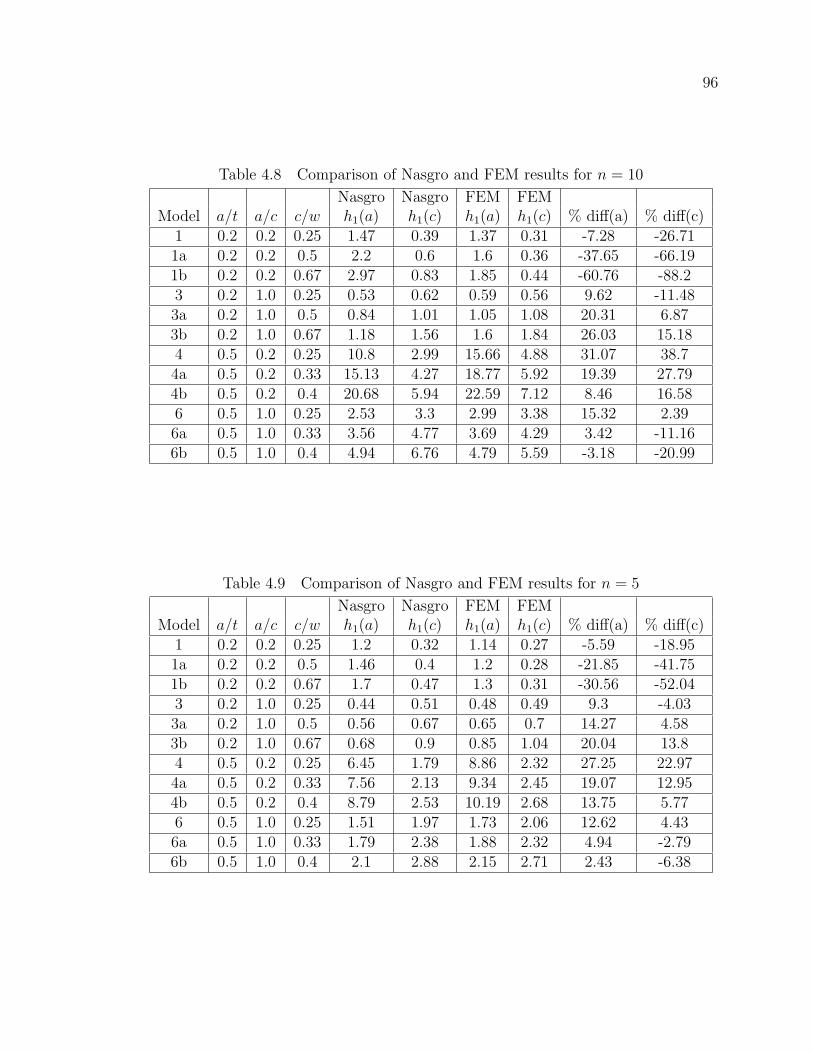
96
Table 4.8 Comparison of Nasgro and FEM results for n = 10
Nasgro Nasgro FEM FEMModel a/t a/c c/w h1(a) h1(c) h1(a) h1(c) % diff(a) % diff(c)
1 0.2 0.2 0.25 1.47 0.39 1.37 0.31 -7.28 -26.711a 0.2 0.2 0.5 2.2 0.6 1.6 0.36 -37.65 -66.191b 0.2 0.2 0.67 2.97 0.83 1.85 0.44 -60.76 -88.23 0.2 1.0 0.25 0.53 0.62 0.59 0.56 9.62 -11.483a 0.2 1.0 0.5 0.84 1.01 1.05 1.08 20.31 6.873b 0.2 1.0 0.67 1.18 1.56 1.6 1.84 26.03 15.184 0.5 0.2 0.25 10.8 2.99 15.66 4.88 31.07 38.74a 0.5 0.2 0.33 15.13 4.27 18.77 5.92 19.39 27.794b 0.5 0.2 0.4 20.68 5.94 22.59 7.12 8.46 16.586 0.5 1.0 0.25 2.53 3.3 2.99 3.38 15.32 2.396a 0.5 1.0 0.33 3.56 4.77 3.69 4.29 3.42 -11.166b 0.5 1.0 0.4 4.94 6.76 4.79 5.59 -3.18 -20.99
Table 4.9 Comparison of Nasgro and FEM results for n = 5
Nasgro Nasgro FEM FEMModel a/t a/c c/w h1(a) h1(c) h1(a) h1(c) % diff(a) % diff(c)
1 0.2 0.2 0.25 1.2 0.32 1.14 0.27 -5.59 -18.951a 0.2 0.2 0.5 1.46 0.4 1.2 0.28 -21.85 -41.751b 0.2 0.2 0.67 1.7 0.47 1.3 0.31 -30.56 -52.043 0.2 1.0 0.25 0.44 0.51 0.48 0.49 9.3 -4.033a 0.2 1.0 0.5 0.56 0.67 0.65 0.7 14.27 4.583b 0.2 1.0 0.67 0.68 0.9 0.85 1.04 20.04 13.84 0.5 0.2 0.25 6.45 1.79 8.86 2.32 27.25 22.974a 0.5 0.2 0.33 7.56 2.13 9.34 2.45 19.07 12.954b 0.5 0.2 0.4 8.79 2.53 10.19 2.68 13.75 5.776 0.5 1.0 0.25 1.51 1.97 1.73 2.06 12.62 4.436a 0.5 1.0 0.33 1.79 2.38 1.88 2.32 4.94 -2.796b 0.5 1.0 0.4 2.1 2.88 2.15 2.71 2.43 -6.38

97
Figure 4.58 Model 1 (a/t = 0.2, a/c = 0.2): h1 vs. c/w for Nasgro and FEM atn = 15
Figure 4.59 Model 1 (a/t = 0.2, a/c = 0.2): h1 vs. c/w for Nasgro and FEM atn = 10

98
Figure 4.60 Model 1 (a/t = 0.2, a/c = 0.2): h1 vs. c/w for Nasgro and FEM atn = 5
Figure 4.61 Model 3 (a/t = 0.2, a/c = 1.0): h1 vs. c/w for Nasgro and FEM atn = 15

99
Figure 4.62 Model 3 (a/t = 0.2, a/c = 1.0): h1 vs. c/w for Nasgro and FEM atn = 10
Figure 4.63 Model 3 (a/t = 0.2, a/c = 1.0): h1 vs. c/w for Nasgro and FEM atn = 5

100
Figure 4.64 Model 4 (a/t = 0.5, a/c = 0.2): h1 vs. c/w for Nasgro and FEM atn = 15
Figure 4.65 Model 4 (a/t = 0.5, a/c = 0.2): h1 vs. c/w for Nasgro and FEM atn = 10
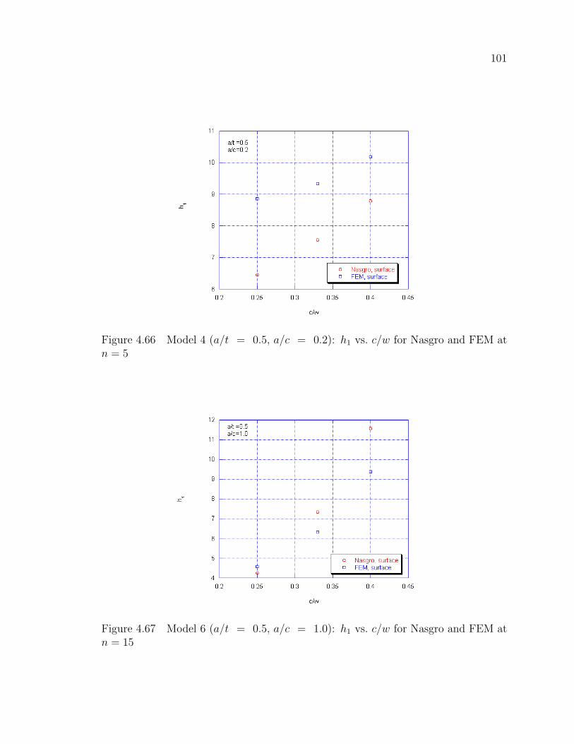
101
Figure 4.66 Model 4 (a/t = 0.5, a/c = 0.2): h1 vs. c/w for Nasgro and FEM atn = 5
Figure 4.67 Model 6 (a/t = 0.5, a/c = 1.0): h1 vs. c/w for Nasgro and FEM atn = 15

102
Figure 4.68 Model 6 (a/t = 0.5, a/c = 1.0): h1 vs. c/w for Nasgro and FEM atn = 10
Figure 4.69 Model 6 (a/t = 0.5, a/c = 1.0): h1 vs. c/w for Nasgro and FEM atn = 5

103
The differences between the current FEM and Nasgro results were varied.
Some geometries produced relatively close comparisons (less than 5%) between the
Nasgro and FEM results. Others demonstrated significant differences (greater than
100%). The differences are most likely a result of the reference stress algorithm used
within Nasgro. This is not to say that the Nasgro results are less correct than the
current FEM results, and no final judgement is made here.
It was also found that no two comparisons of FEM and Nasgro results demon-
strated exactly the same pattern. The specific observations are:
• Model 1 (a/t = 0.2, a/c = 0.2): The Nasgro results were higher for every
tested c/w at all n’s. The difference between the Nasgro and FEM results
increased with c/w for all n’s.
• Model 3 (a/t = 0.2, a/c = 1.0): The FEM results were higher for every
tested c/w at all n’s. The difference between the Nasgro and FEM results
increased with c/w for all n’s.
• Model 4 (a/t = 0.5, a/c = 0.2): The FEM results were higher for every
tested c/w at all n’s. The difference between the Nasgro and FEM results
increased with c/w for n = 10. The difference between the Nasgro and
FEM results decreased as c/w increased for n = 15 and n = 5.
• Model 6 (a/t = 0.5, a/c = 1.0): The FEM results were higher for every
tested c/w at n = 5. The FEM and Nasgro results cross for n = 15 and
n = 10. The difference between the Nasgro and FEM results increased
with c/w for n = 15. The difference between the Nasgro and FEM results
decreased as c/w increased for n = 10 and n = 5.

CHAPTER 5
CONCLUSIONS AND RECOMMENDATIONS
This chapter contains the conclusions and recommendations for this research.
Conclusions are stated for each of the stated goals of this work. The recommendations
for further work address questions that were not answered during this study.
5.1 Conclusions
The following are conclusions reached in this research for the primary goal
of comparing three-dimensional finite element analysis J-integral results produced in
ABAQUS with work completed by other researchers:
1. The K-factor and elastic J-integral results produced in ABAQUS for this
research compare well with the Newman and Raju [18] calculations and Lei
data, except as noted below.
• There is a spike in the K-factor at the surface for most analyzed
geometries. Models with a very deep crack (a/t = 0.8) have smaller
spikes. The elastic J-integral results presented by Lei [17] showed some
surface spikes, but not to same magnitude as found in this research.
• There is a sudden increase in the K-factor in the depth for geome-
tries that do not have highly elliptical (a/t = 0.2) cracks for quarter
symmetry models. There were no spikes observed for the depth in the
results presented by Lei.
2. The fully plastic J-integral results generated in this research compare rea-
sonably well, for some geometries, with work produced McClung et al. [15]
104

105
and Lei [17]. However, there are some issues with using ABAQUS to cal-
culate the J-integral.
• The same surface and depth issues found in the current elastic FEMs
are also present in the fully plastic models.
• The plastic FEMs from the current research, Lei, and McClung et
al. exhibit an anomaly at the third or fourth angle from the surface.
The value of the angle was dependent on the model and ranged from
2.71◦ to 18◦.
3. The quarter symmetry FEA results presented by McClung et al. and Lei
did not contain surface or depth spikes in the plastic J-integral, as found
in the current FEMs. Possible reasons for this finding are given below.
• Other researchers used a smoothing method.
• There was an issue with the quarter symmetry FEMs used in this
research, probably related to the boundary conditions.
4. FEM and Nasgro results compared well for some, but not all, specimen
geometries. There was no apparent pattern to the variation.
The second goal of this research was to investigate the effects of mesh density,
element type, symmetry, and specimen size effects on the J-integral. Based on this
research, the conclusions are made.
1. The schemes used by ABAQUS to calculate K and J are robust and do
not require a significant amount of mesh refinement to produce converged
results.
2. A refined mesh can result in oscillations of the calculated J-integral, espe-
cially at larger n values.

106
3. Reduced integration elements give more consistent results for K-factor and
J-integral calculations in ABAQUS. Full integration elements tend to os-
cillate.
4. Quarter symmetry models experience a spike in the depth. Half symmetry
models do not have the same issue.
5. Specimen height has no significant effect on the J-integral for uniform ten-
sile loading.
6. Specimen width has a very significant effect on the J-integral for uniform
tensile loading.
The third goal of this research was to compare elastic-plastic and fully plastic
results. For the elastic-plastic FEAs, the stress vs. plastic strain table was based
on the Ramberg-Osgood material properties. The elastic-plastic and fully plastic
results compared very well at sufficiently large stresses. The same surface and depth
phenomenon observed in the fully plastic FEMs were also present in the elastic-plastic
results.
5.2 Recommendations
The following recommendations for continuing this research are given.
1. Investigate the surface and depth phenomenon within ABAQUS to answer
these questions:
• Why does ABAQUS yield a spike in the K-factor and J-integral at
the free surface?
• How far into the depth does the surface phenomenon affect results?
• Why do quarter symmetry models have an increase in the depth?

107
2. Investigate the anomaly exhibited by some models at the third and fourth
angles from the surface.
3. Use the existing models to obtain results for corner cracks. This work can
be easily performed by changing the boundary conditions of the existing
models.

REFERENCES
108

109
[1] Griffith, A.A., “The Phenomena of Rupture and Flow in Solids.” PhilosophicalTransactions, Series A, Vol. 221, 1920, pp. 163-198.
[2] Irwin, G.R., “Fracture Dynamics.” Fracturing of Metals, American Society forMetals, Cleveland, 1948, pp. 147-166.
[3] Irwin, G.R., “Analysis of Stresses and Strains near the End of a Crack Travers-ing a Plate.” Journal of Applied Mechanics, Vol. 24, 1957, pp. 361-364.
[4] Anderson, T. L., Fracture Mechanics Fundamentals and Applications, SecondEdition, CRC Press, FL, 1991.
[5] Tada, H, P.C. Paris, and G.R. Irwin, The Stress Analysis of Cracks Handbook,ASME Press, New York, 2000.
[6] Wells, A.A., “Unstable Crack Propagation in Metals: Cleavage and Fast Frac-ture.” Proceedings of the Crack Propagation Symposium, Vol. 1, Paper 84,Cranfield UK, 1961.
[7] Rice, J.R. “A Path Independent Integral and the Approximate Analysis ofStrain Concentraion by Notches and Cracks.” Journal of Applied Mechanics,Vol. 35, 1968, pp. 379-386.
[8] Hutchinson, J.W., “Singular Behavior at the End of a Tensile Crack Tip in aHardening Material.” Journal of the Mechanics and Physics of Solids, Vol. 16,1968, pp.13-31.
[9] Rice, J.R. and G.F. Rosengren, “Plane Strain Deformation Near a Crack Tipin a Power-Law Hardening Material.” Journal of the Mechanics and Physics ofSolids, Vol. 16, 1968, pp. 1-12.
[10] Cook, R.D., D.S. Malkus, M.E. Plesha, R.J. Witt, Concepts and Applicationsof Finite Element Analysis, Fourth Edition, John Wiley & Sons, Inc., 2002.
[11] Kumar, V., M.D. German, and C.F. Shih, “An Engineering Approach forElastic-Plastic Fracture Analysis,” Report NP-1931, Electric Power ResearchInstitute, 1981.
[12] Shih, C.F., “J-Integral Estimates for Strain Hardening Materials in AntiplaneShear Using Fully Plastic Solutions,” in Mechanics of Crack Growth, ASTMSpecial Publication 590, 1976, pp. 3-22.

110
[13] Shih, C.F., and J.W. Hutchinson, “Fully Plastic Solutions and Large-ScaleYielding Estimates for Plane Stress Crack Problems,” Transactions of ASME,Journal of Engineering Materials and Technology, Series H, Vol.98, October1976, pp. 289-295.
[14] Needleman, A., and C.F. Shih, “A Finite Element Method for Plane Strain De-formations of Incompressible Solids.” Computer Methods in Applied Mechanicsand Engineering, 1978, pp. 223-240.
[15] McClung, R.C., G.G. Chell, Y.D. Lee, D.A. Russell, and G.E. Orient, 1999,“Developement of a Practical Methodology for Elastic-Plastic and Fully Plas-tic Fatigue Crack Growth,” National Aeronautics and Space Administration,Marshall Space Flight Center, Alabama, Contract NAS8-37828.
[16] ABAQUS Analysis User’s Manual Version 6.4, ABAQUS, Inc., 2003.
[17] Lei, Y., “J-integral and limit load analysis of semi-elliptical surface cracks inplates under tension.” International Journal of Pressure Vessels and Piping,2004, pp. 21-31.
[18] Newman, J.C. and Raju, I.S., “An empirical stress-intensity factor equation forthe surface crack.” Engineering Fracture Mechanics, 1981, pp. 185-192.
[19] Ainsworth, R.A., “The Assessment of Defects in Structures of Strain HardeningMaterials.” Engineering Fracture Mechanics, Vol. 19, 1984, p.633.
[20] Faleskog, Jonas, User’s Manual: mesh3d scp, 1996.
[21] ABAQUS User’s Manual, Version ???.
[22] Natarajan, Krishna R., Plastic J-Integral Solutions for Through Cracks Us-ing Finite Element Method, Master of Science Thesis, Tennessee TechnologicalUniversity, Cookeville, TN.
[23] Kirk, M.T. and R.H. Dodds, “Approximate Techniques of J Estimation Appli-cable to Part-Though Surface Cracks,” Engineering Fracture Mechanics, Vol.43, No. 1, 1992, pp. 123-136.

111
[24] Newman, J.C. and Raju, I.S., “Stress Intensity Factor Equations for Cracks inThree-Dimensional Finite Bodies”, Fracture Mechanics: Fourteenth Symposium- Volume 1: Theory and Analysis, ASTM STP 791, J. C. Lewis and G. Sines,Eds.,American Society for Testing and Materials, 1983, pp. I-238 - I-265.
[25] Newman, J.C. and Raju, I.S., “Analysis of Surface Cracks in Finite PlatesUnder Tension of Bending Loads,” NASA Technical Paper 1578, Dec. 1979.
[26] “3D Finite Element Software for Cracks, Version 2.5, Benchmarks and Valida-tion,” Structural Reliability Technology, Boulder, CO, July, 2003.
[27] Computational Fracture Mechanics Group at University of Illinois Urbana-Champaign, http://cern49.ce.uiuc.edu/cfm/warp3d.html, accessed 1-31-2005.
[28] Lloyd, W.R., and W.G. Reuter, “Evaluation of Elastic-Plastic Surface FlawBehavior and Related Parameters Using Surface Displacement Measurements,”Fracture Mechanics: Twenty-First Symposium, ASTM STP 1074, J.P. Gudas,J.A. Joyce, and E.M. Hackett, Eds., American Society for Testing and Materi-als, Philadelphia, 1990, pp. 322-336.
[29] Irwin, G.R., “Plastic Zone Near a Crack and Fracture Toughness,” SagamoreResearch Conference Proceedings, Vol. 4, 1961.
[30] Dodds, R. H. Jr. and David T. Read, “Experimental and Numerical Studies ofthe J-Integral for a Surface Flaw,” International Journal of Fracture, Vol. 43,1990, pp. 47-67.
[31] Read,D.T., “Applied J-Integral in HY-130 Tensile Panels and Implications forFitness for Service Assessment,” Report NBSIR 82-1670, National Bureau ofStandards, Boulder, CO, 1982.
[32] Yagawa, G., Y. Kitajima, H. Ueda, “Three-Dimensional Fully Plastic Solutionsfor Semi-elliptical Surface Cracks,” International Journal of Pressure Vesselsand Piping, Vol. 53, 1993, pp. 457-510.

APPENDICES
112

APPENDIX A: INSTRUCTIONS FOR MESH3D SCPMODIFICATIONS
113

114
1. Insure that the correct element type (8, 20, or 27-node) is specified in themesh3d scp input file. This is done by changing the “ETYP=??” field tothe appropriate value.
2. The mesh3d scp program creates several files when run. Three of thesecontain node and element data. The file names are described below:• test.015 - contains node and coordinate data• test.016 - contains element connectivities• test.017 - contains element connectivities
Use the following steps to modify these files for use with ABAQUS 6.5.(a) Combine test.016 and test.017 using cat test.016 test.017 > temp ele.inp.(b) At the top of temp ele.inp, add *ELEMENT, TYPE=C3D20R,ELSET=
ELEMALL.(c) Run abaqus free job=elements input=temp ele
3. Change the node file name from test.015 to nodes.inp.4. Insert the *NODE at the top of the nodes.inp file.5. Make the following changes to the test.inp file (input file for ABAQUS):
• There will be three lines referencing test.015 thru test.017. Deletethese lines.
• Add *INCLUDE, INPUT=nodes.inp• Add *INCLUDE, INPUT=elements.inp• At the bottom of the file, add comma’s to the spaces between the
contours in the *CONTOUR INTEGRAL command.• Many, but not all, of the commands between *MATERIAL and
*****STEP=1****** are not valid and should be replaced withthe appropriate commands.

APPENDIX B: COARSE VERSUS REFINED MESHES FORK-FACTORS
115

116
Figure B.1 Model 1 (a/t=0.2, a/c=0.2): Normalized K factor vs. angle alongcrack front
Figure B.2 Model 2 (a/t=0.2, a/c=0.6): Normalized K factor vs. angle alongcrack front

117
Figure B.3 Model 3 (a/t=0.2, a/c=1.0): Normalized K factor vs. angle alongcrack front
Figure B.4 Model 4 (a/t=0.5, a/c=0.2): Normalized K factor vs. angle alongcrack front

118
Figure B.5 Model 5 (a/t=0.5, a/c=0.6): Normalized K factor vs. angle alongcrack front
Figure B.6 Model 6 (a/t=0.5, a/c=1.0): Normalized K factor vs. angle alongcrack front

119
Figure B.7 Model 8 (a/t=0.8, a/c=0.6): Normalized K factor vs. angle alongcrack front
Figure B.8 Model 9 (a/t=0.8, a/c=1.0): Normalized K factor vs. angle alongcrack front

APPENDIX C: COARSE VS. REFINED MESHES FOR FULLYPLASTIC MODELS
120

121
Figure C.9 Model 1: h1 vs. angle along the crack front
Figure C.10 Model 1: h1 vs. angle along the crack front

122
Figure C.11 Model 1: h1 vs. angle along the crack front
Figure C.12 Model 2: h1 vs. angle along the crack front

123
Figure C.13 Model 2: h1 vs. angle along the crack front
Figure C.14 Model 2: h1 vs. angle along the crack front

124
Figure C.15 Model 3: h1 vs. angle along the crack front
Figure C.16 Model 3: h1 vs. angle along the crack front

125
Figure C.17 Model 3: h1 vs. angle along the crack front
Figure C.18 Model 4: h1 vs. angle along the crack front

126
Figure C.19 Model 4: h1 vs. angle along the crack front
Figure C.20 Model 4: h1 vs. angle along the crack front

127
Figure C.21 Model 5: h1 vs. angle along the crack front
Figure C.22 Model 5: h1 vs. angle along the crack front
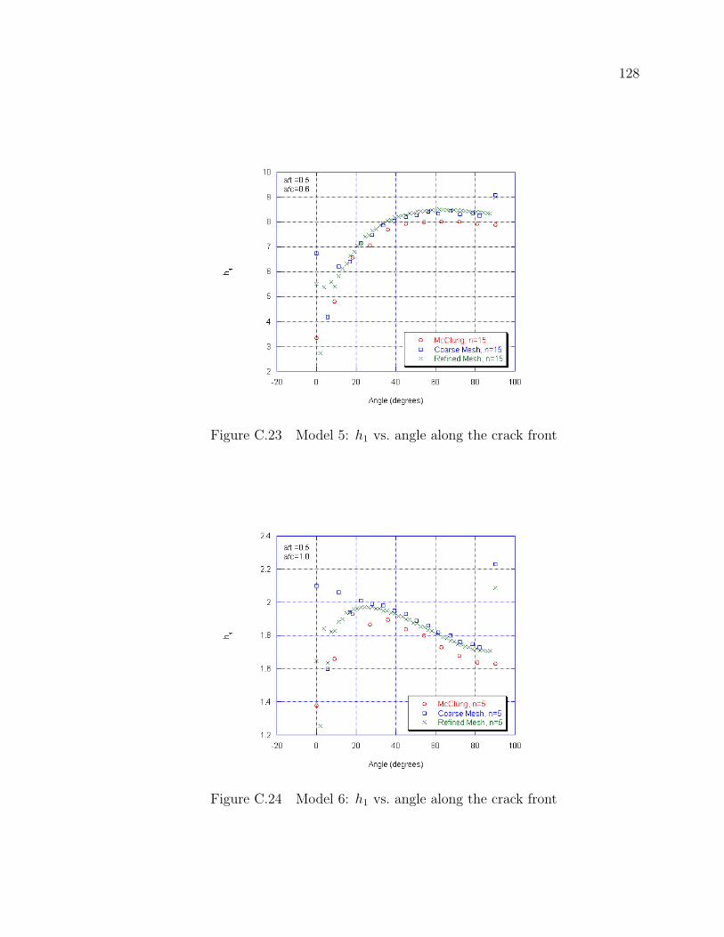
128
Figure C.23 Model 5: h1 vs. angle along the crack front
Figure C.24 Model 6: h1 vs. angle along the crack front

129
Figure C.25 Model 6: h1 vs. angle along the crack front
Figure C.26 Model 6: h1 vs. angle along the crack front

130
Figure C.27 Model 8: h1 vs. angle along the crack front
Figure C.28 Model 8: h1 vs. angle along the crack front

131
Figure C.29 Model 8: h1 vs. angle along the crack front
Figure C.30 Model 9: h1 vs. angle along the crack front

132
Figure C.31 Model 9: h1 vs. angle along the crack front
Figure C.32 Model 9: h1 vs. angle along the crack front

APPENDIX D: HEIGHT EFFECTS
133

134
Table D.1 Model 4 (a/t=0.5 and a/c=0.2): h1 values for at different heights (Part1)
θ h/w = 1 h/w = 3 h/w = 50.00 33.58 33.42 33.493.04 16.67 16.65 16.686.10 23.62 23.62 23.679.00 27.80 27.79 27.8611.93 30.36 30.33 30.3914.60 34.61 34.55 34.6217.30 36.76 36.65 36.7319.73 40.42 40.27 40.3522.19 42.86 42.66 42.7424.25 45.91 45.64 45.7326.35 48.64 48.32 48.4028.23 51.13 50.77 50.8530.15 54.08 53.66 53.7531.88 55.60 55.12 55.2033.64 57.94 57.39 57.4835.24 59.64 59.05 59.1236.87 61.04 60.39 60.4639.40 63.83 63.09 63.1842.02 66.02 65.22 65.2844.32 67.30 66.41 66.4846.71 69.30 68.37 68.4548.83 69.82 68.81 68.8851.06 71.45 70.41 70.4853.05 71.79 70.69 70.7655.15 72.77 71.62 71.7057.05 73.12 71.93 71.9959.05 73.77 72.54 72.6260.87 74.00 72.76 72.8162.80 74.68 73.41 73.4964.55 74.51 73.18 73.2466.42 75.40 74.06 74.1368.12 74.83 73.51 73.5769.95 75.53 74.15 74.21

135
Table D.2 Model 4 (a/t=0.5 and a/c=0.2): h1 values for at different heights (Part2)
θ h/w = 1 h/w = 3 h/w = 571.60 75.13 73.76 73.8273.40 75.50 74.12 74.1875.00 75.22 73.83 73.9076.79 75.57 74.16 74.2178.34 75.26 73.85 73.9180.13 75.62 74.20 74.2681.62 75.28 73.84 73.9083.44 75.63 74.19 74.2684.81 75.33 73.88 73.9486.72 75.65 74.19 74.2587.68 75.33 73.87 73.9490.00 76.26 74.78 74.84
Table D.3 Model 5 (a/t=0.5 and a/c=0.6): h1 values for at different heights
θ h/w = 1 h/w = 3 h/w = 50.00 4.74 4.58 4.585.60 2.97 2.89 2.8811.25 4.43 4.32 4.3216.79 4.58 4.46 4.4622.50 5.10 4.97 4.9627.98 5.34 5.19 5.1833.75 5.62 5.45 5.4439.15 5.73 5.55 5.5445.00 5.85 5.67 5.6650.29 5.91 5.71 5.7056.25 6.00 5.79 5.7861.36 5.95 5.74 5.7367.50 6.02 5.79 5.7872.24 5.94 5.71 5.7078.75 5.97 5.74 5.7382.05 5.90 5.67 5.6690.00 6.51 6.26 6.25

136
Table D.4 Model 9 (a/t=0.8 and a/c=1.0): h1 values for at different heights
θ h/w = 1 h/w = 3 h/w = 50.00 7.27 6.95 6.945.60 9.35 8.99 8.9711.25 12.88 12.39 12.3716.79 12.19 11.81 11.7922.50 13.33 12.88 12.8627.98 12.87 12.42 12.4033.75 12.50 12.06 12.0439.15 11.76 11.33 11.3145.00 10.99 10.55 10.5350.29 10.37 10.01 9.9956.25 9.96 9.58 9.5661.36 9.53 9.16 9.1467.50 9.27 8.88 8.8672.24 9.27 8.83 8.8178.75 9.35 8.95 8.9282.05 9.22 8.78 8.7690.00 10.12 9.71 9.68

APPENDIX E: K-FACTOR RESULTS FOR COARSE MESHES
137

138
Tab
leE
.5M
odel
1(a
/t=
0.2,
a/c=
0.2)
:K
-Fac
tor
dat
afr
omA
BA
QU
S(P
art
1)
Angl
eN
ewm
an-R
aju
FE
AK
FE
AK
FE
AK
Dir
ectl
y%
diff
%diff
%diff
(deg
rees
)D
irec
tly
from
Jel
Tie
dN
odes
FE
AD
irec
tfr
omJ
elT
ied
Nodes
0.00
0.59
0.85
0.81
0.83
44.1
337
.15
40.9
33.
040.
600.
590.
590.
59-1
.16
-1.5
2-0
.74
6.10
0.62
0.58
0.59
0.56
-5.6
3-4
.86
-8.5
09.
000.
640.
610.
620.
62-4
.64
-4.5
0-4
.24
11.9
30.
680.
640.
640.
63-5
.64
-5.3
8-7
.29
14.6
00.
710.
670.
670.
68-5
.35
-5.2
2-5
.17
17.3
00.
750.
710.
710.
70-5
.30
-5.1
8-6
.30
19.7
30.
780.
740.
740.
74-5
.15
-5.0
5-5
.13
22.1
90.
800.
770.
770.
76-4
.83
-4.7
5-5
.62
24.2
50.
830.
790.
790.
79-4
.95
-4.8
6-4
.93
26.3
50.
850.
810.
810.
81-4
.49
-4.4
0-5
.10
28.2
30.
870.
830.
830.
83-4
.58
-4.4
9-4
.55
30.1
50.
890.
850.
850.
85-4
.09
-4.0
0-4
.65
31.8
80.
910.
870.
870.
87-4
.31
-4.2
3-4
.25
33.6
40.
920.
890.
890.
89-3
.43
-3.3
4-4
.10
35.2
40.
940.
900.
900.
90-4
.42
-4.3
2-4
.34
36.8
70.
950.
920.
930.
92-2
.95
-2.9
0-3
.26
41.6
00.
990.
970.
970.
97-2
.33
-2.2
0-2
.35

139
Tab
leE
.6M
odel
1(a
/t=
0.2,
a/c=
0.2)
:K
-Fac
tor
dat
afr
omA
BA
QU
S(P
art
2)
Angl
eN
ewm
an-R
aju
FE
AK
FE
AK
FE
AK
Dir
ectl
y%
diff
%diff
%diff
(deg
rees
)D
irec
tly
from
Jel
Tie
dN
odes
FE
AD
irec
tfr
omJ
elT
ied
Nodes
46.7
11.
031.
011.
011.
00-2
.44
-2.3
8-2
.60
50.7
41.
061.
041.
041.
04-2
.01
-1.9
1-2
.07
55.1
51.
081.
061.
071.
06-1
.85
-1.7
9-2
.05
58.7
61.
101.
091.
091.
08-1
.74
-1.6
6-1
.81
62.8
01.
121.
111.
111.
10-1
.63
-1.5
6-1
.82
66.1
21.
141.
121.
121.
12-1
.59
-1.5
2-1
.65
69.9
51.
151.
141.
141.
13-1
.51
-1.4
5-1
.70
73.0
31.
161.
151.
151.
14-1
.52
-1.4
5-1
.59
76.7
91.
171.
161.
161.
15-1
.48
-1.4
0-1
.63
79.5
71.
181.
161.
161.
16-1
.49
-1.4
2-1
.55
83.4
41.
181.
171.
171.
16-1
.46
-1.3
8-1
.61
85.3
61.
191.
171.
171.
17-1
.48
-1.4
1-1
.55
90.0
01.
191.
181.
181.
18-0
.90
-0.8
8-1
.05

140
Tab
leE
.7M
odel
2(a
/t=
0.2,
a/c=
0.6)
:K
-Fac
tor
dat
afr
omA
BA
QU
S
Angl
eN
ewm
an-R
aju
FE
AK
FE
AK
%diff
%diff
(deg
rees
)D
irec
tly
from
Jel
FE
AD
irec
tfr
omJ
el
0.00
0.96
1.25
1.21
30.5
226
.62
5.60
0.94
0.94
0.94
0.00
-0.3
011
.25
0.94
0.92
0.93
-1.7
4-1
.14
16.7
90.
940.
930.
93-1
.70
-1.5
922
.50
0.95
0.93
0.93
-2.2
5-1
.88
27.9
80.
960.
940.
95-1
.89
-1.7
633
.75
0.98
0.96
0.96
-2.0
4-1
.74
39.1
51.
000.
980.
98-1
.87
-1.7
445
.00
1.02
1.00
1.00
-1.9
1-1
.69
50.2
91.
031.
011.
01-1
.90
-1.7
756
.25
1.05
1.03
1.03
-1.9
4-1
.75
61.3
61.
071.
041.
05-2
.02
-1.9
067
.50
1.08
1.06
1.06
-2.0
6-1
.90
72.2
41.
091.
071.
07-2
.17
-2.0
678
.75
1.10
1.08
1.08
-2.2
1-2
.05
82.0
51.
101.
081.
08-2
.28
-2.1
890
.00
1.11
1.16
1.14
4.55
3.44

141
Tab
leE
.8M
odel
3(a
/t=
0.2,
a/c=
1.0)
:K
-Fac
tor
dat
afr
omA
BA
QU
S
Angl
eN
ewm
an-R
aju
FE
AK
FE
AK
%diff
%diff
(deg
rees
)D
irec
tly
from
Jel
FE
AD
irec
tfr
omJ
el
0.00
1.18
1.44
1.41
22.0
819
.76
5.60
1.15
1.19
1.19
3.11
2.88
11.2
51.
131.
161.
172.
402.
8116
.79
1.12
1.14
1.14
1.62
1.70
22.5
01.
101.
121.
121.
201.
5327
.98
1.09
1.10
1.10
1.22
1.33
33.7
51.
081.
091.
090.
981.
3139
.30
1.07
1.08
1.08
1.05
1.19
44.9
21.
071.
081.
080.
851.
1650
.54
1.06
1.07
1.07
0.83
0.99
56.1
51.
061.
071.
070.
650.
9461
.77
1.06
1.06
1.07
0.55
0.72
67.3
91.
061.
061.
060.
390.
6773
.00
1.06
1.06
1.06
0.25
0.44
78.6
21.
061.
061.
060.
170.
4484
.24
1.06
1.06
1.06
0.13
0.28
90.0
01.
061.
281.
2321
.22
16.2
3

142
Tab
leE
.9M
odel
4(a
/t=
0.5,
a/c=
0.2)
:K
-Fac
tor
dat
afr
omA
BA
QU
S(P
art
1)
Angl
eN
ewm
an-R
aju
FE
AK
FE
AK
%diff
%diff
(deg
rees
)D
irec
tly
from
Jel
FE
AD
irec
tfr
omJ
el
0.00
0.82
1.17
1.10
42.5
235
.03
3.04
0.82
0.80
0.80
-2.2
4-2
.56
6.10
0.84
0.78
0.79
-6.4
0-5
.57
9.00
0.87
0.83
0.83
-5.0
7-4
.91
11.9
30.
910.
860.
86-5
.70
-5.3
714
.60
0.95
0.90
0.90
-5.0
9-4
.95
17.3
00.
990.
940.
94-4
.74
-4.5
619
.73
1.02
0.98
0.98
-4.3
4-4
.21
22.1
91.
051.
011.
02-3
.78
-3.6
724
.25
1.08
1.04
1.04
-3.6
3-3
.51
26.3
51.
111.
081.
08-2
.96
-2.8
728
.23
1.13
1.10
1.10
-2.7
7-2
.67
30.1
51.
151.
131.
13-2
.19
-2.1
031
.88
1.17
1.15
1.15
-2.0
2-1
.92
33.6
41.
191.
181.
18-1
.36
-1.2
735
.24
1.21
1.19
1.19
-1.3
8-1
.28
36.8
71.
231.
221.
22-0
.79
-0.7
339
.40
1.25
1.25
1.25
-0.2
3-0
.12
42.0
21.
281.
281.
280.
020.
1144
.32
1.30
1.30
1.31
0.53
0.62
46.7
11.
321.
331.
330.
870.
9548
.83
1.34
1.35
1.35
1.18
1.25
51.0
61.
351.
371.
371.
491.
56

143
Tab
leE
.10
Model
4(a
/t=
0.5,
a/c=
0.2)
:K
-Fac
tor
dat
afr
omA
BA
QU
S(P
art
2)
Angl
eN
ewm
an-R
aju
FE
AK
FE
AK
%diff
%diff
(deg
rees
)D
irec
tly
from
Jel
FE
AD
irec
tfr
omJ
el
53.0
51.
371.
391.
391.
721.
7955
.15
1.38
1.41
1.41
1.97
2.03
57.0
51.
401.
431.
432.
152.
2159
.05
1.41
1.44
1.44
2.35
2.41
60.8
71.
421.
461.
462.
482.
5462
.80
1.43
1.47
1.47
2.66
2.71
64.5
51.
441.
481.
482.
762.
8266
.42
1.45
1.49
1.49
2.88
2.92
68.1
21.
461.
501.
502.
932.
9969
.95
1.47
1.51
1.51
3.03
3.08
71.6
01.
471.
521.
523.
103.
1573
.40
1.48
1.53
1.53
3.17
3.22
75.0
01.
491.
531.
533.
213.
2676
.79
1.49
1.54
1.54
3.26
3.31
78.3
41.
491.
541.
543.
293.
3380
.13
1.50
1.55
1.55
3.33
3.37
81.6
21.
501.
551.
553.
343.
3983
.44
1.50
1.56
1.56
3.37
3.41
84.8
11.
511.
561.
563.
383.
4286
.72
1.51
1.56
1.56
3.39
3.43
87.6
81.
511.
561.
563.
393.
4390
.00
1.51
1.57
1.57
3.76
3.79

144
Tab
leE
.11
Model
5(a
/t=
0.5,
a/c=
0.6)
:K
-Fac
tor
dat
afr
omA
BA
QU
S
Angl
eN
ewm
an-R
aju
FE
AK
FE
AK
%diff
%diff
(deg
rees
)D
irec
tly
from
Jel
FE
AD
irec
tfr
omJ
el
0.00
1.13
1.40
1.37
24.1
421
.54
5.60
1.10
1.12
1.12
2.15
1.82
11.2
51.
081.
091.
090.
481.
0716
.79
1.08
1.08
1.08
0.55
0.65
22.5
01.
081.
081.
080.
130.
4527
.98
1.08
1.09
1.09
0.40
0.49
33.7
51.
101.
101.
100.
280.
5039
.15
1.11
1.11
1.11
0.24
0.32
45.0
01.
131.
131.
130.
050.
2250
.29
1.15
1.14
1.14
-0.2
3-0
.16
56.2
51.
161.
161.
16-0
.52
-0.3
961
.36
1.18
1.17
1.17
-0.9
2-0
.86
67.5
01.
191.
181.
18-1
.24
-1.1
272
.24
1.20
1.19
1.19
-1.6
0-1
.56
78.7
51.
221.
191.
19-1
.83
-1.7
282
.05
1.22
1.19
1.20
-2.0
1-1
.96
90.0
01.
221.
261.
252.
651.
97

145
Tab
leE
.12
Model
6(a
/t=
0.5,
a/c=
1.0)
:K
-Fac
tor
dat
afr
omA
BA
QU
S
Angl
eN
ewm
an-R
aju
FE
AK
FE
AK
%diff
%diff
(deg
rees
)D
irec
tly
from
Jel
FE
AD
irec
tfr
omJ
el
0.00
1.31
1.52
1.50
16.0
914
.64
5.60
1.27
1.32
1.31
3.35
3.10
11.2
51.
241.
281.
283.
063.
4416
.79
1.21
1.24
1.24
2.53
2.63
22.5
01.
181.
211.
222.
482.
7227
.98
1.16
1.19
1.19
2.54
2.64
33.7
51.
151.
171.
182.
482.
7439
.15
1.13
1.16
1.16
2.44
2.55
45.0
01.
121.
151.
152.
242.
4950
.29
1.12
1.14
1.14
2.02
2.14
56.2
51.
111.
131.
131.
701.
9461
.36
1.11
1.12
1.12
1.36
1.49
67.5
01.
111.
121.
121.
021.
2672
.24
1.11
1.11
1.11
0.72
0.84
78.7
51.
111.
111.
110.
490.
7182
.05
1.11
1.11
1.11
0.36
0.45
90.0
01.
111.
271.
2415
.10
11.9
5

146
Tab
leE
.13
Model
7(a
/t=
0.8,
a/c=
0.2)
:K
-Fac
tor
dat
afr
omA
BA
QU
S(P
art
1)
Angl
eN
ewm
an-R
aju
FE
AK
FE
AK
%diff
%diff
(deg
rees
)D
irec
tly
from
Jel
FE
AD
irec
tfr
omJ
el
0.00
1.19
1.49
1.46
25.7
523
.29
2.44
1.17
1.23
1.22
4.52
4.07
4.88
1.18
1.19
1.20
0.62
1.29
7.20
1.21
1.22
1.22
0.90
0.98
9.53
1.25
1.24
1.25
-0.1
90.
0011
.64
1.28
1.28
1.28
-0.0
8-0
.03
13.7
71.
321.
321.
32-0
.06
0.01
15.6
81.
351.
351.
350.
010.
0317
.61
1.39
1.39
1.39
0.36
0.39
19.2
21.
411.
421.
420.
320.
3220
.84
1.44
1.45
1.45
0.94
0.95
22.3
11.
461.
481.
481.
021.
0023
.79
1.49
1.51
1.51
1.57
1.55
25.1
21.
511.
531.
531.
621.
6226
.48
1.53
1.56
1.56
2.26
2.26
27.7
11.
541.
581.
582.
212.
2028
.96
1.56
1.60
1.60
2.76
2.73
30.6
91.
581.
631.
633.
153.
1432
.46
1.61
1.66
1.66
3.30
3.27
34.0
51.
631.
691.
693.
663.
6435
.66
1.65
1.71
1.71
3.88
3.86
37.1
31.
661.
731.
734.
044.
0138
.62
1.68
1.75
1.75
4.22
4.18

147
Tab
leE
.14
Model
7(a
/t=
0.8,
a/c=
0.2)
:K
-Fac
tor
dat
afr
omA
BA
QU
S(P
art
2)
Angl
eN
ewm
an-R
aju
FE
AK
FE
AK
%diff
%diff
(deg
rees
)D
irec
tly
from
Jel
FE
AD
irec
tfr
omJ
el
40.0
01.
701.
771.
774.
284.
2441
.41
1.71
1.79
1.78
4.38
4.34
42.7
21.
721.
801.
804.
374.
3344
.05
1.74
1.81
1.81
4.41
4.37
45.2
91.
751.
831.
834.
334.
3046
.57
1.76
1.84
1.84
4.34
4.30
47.7
61.
781.
851.
854.
224.
1748
.99
1.79
1.86
1.86
4.12
4.07
50.1
41.
801.
871.
873.
923.
8651
.32
1.81
1.88
1.88
3.77
3.72
52.4
31.
821.
881.
883.
613.
5453
.58
1.83
1.89
1.89
3.41
3.36
54.6
61.
841.
901.
903.
183.
1255
.77
1.85
1.90
1.90
2.97
2.91
56.8
31.
861.
911.
902.
722.
6557
.91
1.86
1.91
1.91
2.47
2.41
58.9
41.
871.
911.
912.
192.
1260
.00
1.88
1.92
1.92
1.94
1.86
61.0
11.
891.
921.
921.
651.
5762
.05
1.90
1.92
1.92
1.39
1.30
63.0
31.
901.
921.
921.
091.
0164
.06
1.91
1.92
1.92
0.78
0.70
65.0
21.
921.
931.
920.
470.
3966
.03
1.92
1.93
1.92
0.19
0.10
66.9
81.
931.
931.
92-0
.09
-0.1
967
.98
1.93
1.93
1.93
-0.3
7-0
.48

148
Tab
leE
.15
Model
7(a
/t=
0.8,
a/c=
0.2)
:K
-Fac
tor
dat
afr
omA
BA
QU
S(P
art
3)
Angl
eN
ewm
an-R
aju
FE
AK
FE
AK
%diff
%diff
(deg
rees
)D
irec
tly
from
Jel
FE
AD
irec
tfr
omJ
el
68.9
11.
941.
931.
93-0
.68
-0.7
769
.89
1.95
1.93
1.93
-0.9
5-1
.05
70.8
21.
951.
931.
92-1
.22
-1.3
371
.79
1.96
1.93
1.92
-1.4
9-1
.59
72.7
01.
961.
931.
92-1
.75
-1.8
673
.67
1.96
1.93
1.92
-2.0
0-2
.11
74.5
71.
971.
921.
92-2
.25
-2.3
675
.52
1.97
1.92
1.92
-2.4
8-2
.59
76.4
11.
981.
921.
92-2
.70
-2.8
177
.36
1.98
1.92
1.92
-2.9
2-3
.03
78.2
41.
981.
921.
92-3
.13
-3.2
479
.19
1.99
1.92
1.92
-3.3
1-3
.43
80.0
61.
991.
921.
92-3
.47
-3.5
981
.01
1.99
1.92
1.92
-3.6
4-3
.75
81.8
61.
991.
921.
92-3
.78
-3.9
082
.82
1.99
1.92
1.91
-3.9
2-4
.04
83.6
62.
001.
921.
91-4
.03
-4.1
584
.62
2.00
1.92
1.91
-4.1
4-4
.26
85.4
32.
001.
921.
91-4
.22
-4.3
486
.42
2.00
1.91
1.91
-4.3
0-4
.42
87.1
72.
001.
911.
91-4
.34
-4.4
788
.21
2.00
1.91
1.91
-4.4
0-4
.51
88.7
32.
001.
911.
91-4
.41
-4.5
390
.00
2.00
1.92
1.91
-4.2
9-4
.42

149
Tab
leE
.16
Model
8(a
/t=
0.8,
a/c=
0.6)
:K
-Fac
tor
dat
afr
omA
BA
QU
S(P
art
1)
Angl
eN
ewm
an-R
aju
FE
AK
FE
AK
FE
AK
Dir
ectl
y%
diff
%diff
%diff
(deg
rees
)D
irec
tly
from
Jel
Tie
dN
odes
FE
AD
irec
tfr
omJ
elT
ied
Nodes
0.00
1.40
1.53
1.52
1.52
9.52
8.66
8.74
4.03
1.35
1.42
1.41
1.42
4.60
4.38
4.56
8.09
1.32
1.37
1.38
1.36
3.57
4.40
2.95
11.9
71.
291.
331.
341.
343.
193.
283.
2715
.92
1.27
1.31
1.31
1.30
2.69
3.10
2.07
19.5
51.
261.
301.
301.
302.
682.
782.
7823
.26
1.25
1.29
1.29
1.28
2.50
2.77
1.94
26.6
21.
251.
281.
281.
282.
392.
472.
4730
.09
1.25
1.28
1.28
1.27
2.26
2.43
1.75
33.0
01.
251.
271.
271.
271.
811.
901.
9136
.02
1.25
1.28
1.28
1.27
1.88
1.98
1.40
38.7
21.
261.
271.
281.
281.
331.
411.
4241
.52
1.26
1.28
1.28
1.27
1.23
1.29
0.79
44.0
21.
271.
281.
281.
280.
560.
640.
6446
.62
1.27
1.28
1.28
1.28
0.60
0.62
0.14
48.9
51.
281.
271.
271.
27-0
.45
-0.4
5-0
.48

150
Tab
leE
.17
Model
8(a
/t=
0.8,
a/c=
0.6)
:K
-Fac
tor
dat
afr
omA
BA
QU
S(P
art
2)
Angl
eN
ewm
an-R
aju
FE
AK
FE
AK
FE
AK
Dir
ectl
y%
diff
%diff
%diff
(deg
rees
)D
irec
tly
from
Jel
Tie
dN
odes
FE
AD
irec
tfr
omJ
elT
ied
Nodes
51.3
91.
291.
281.
281.
28-0
.49
-0.5
0-0
.86
54.4
01.
291.
281.
281.
28-1
.09
-1.0
4-1
.02
57.6
61.
301.
271.
281.
27-2
.20
-2.1
2-2
.41
60.4
61.
311.
281.
281.
28-2
.69
-2.6
6-2
.68
63.5
31.
321.
271.
281.
27-3
.40
-3.3
6-3
.66
66.1
61.
331.
271.
271.
27-4
.04
-4.0
2-4
.03
69.1
11.
331.
271.
271.
27-4
.64
-4.6
1-4
.89
71.6
11.
341.
271.
271.
27-5
.20
-5.1
8-5
.20
74.4
91.
351.
271.
271.
27-5
.67
-5.6
7-5
.92
76.8
51.
351.
271.
271.
27-6
.12
-6.1
1-6
.12
79.7
31.
351.
271.
271.
26-6
.45
-6.4
5-6
.69
81.8
91.
361.
261.
261.
26-6
.75
-6.7
5-6
.75
84.8
91.
361.
261.
261.
26-6
.93
-6.9
3-7
.17
86.3
81.
361.
261.
261.
26-7
.07
-7.0
7-7
.07
90.0
01.
361.
281.
281.
28-5
.74
-5.9
1-5
.97

151
Tab
leE
.18
Model
9(a
/t=
0.8,
a/c=
1.0)
:K
-Fac
tor
dat
afr
omA
BA
QU
S
Angl
eN
ewm
an-R
aju
FE
AK
FE
AK
%diff
%diff
(deg
rees
)D
irec
tly
from
Jel
FE
AD
irec
tfr
omJ
el
0.00
1.54
1.59
1.59
3.54
3.51
5.60
1.47
1.50
1.50
2.12
2.03
11.2
51.
411.
441.
442.
352.
7016
.79
1.35
1.38
1.38
2.15
2.25
22.5
01.
311.
341.
342.
572.
8227
.98
1.27
1.30
1.30
2.65
2.76
33.7
51.
241.
271.
272.
803.
0339
.15
1.21
1.24
1.24
2.46
2.56
45.0
01.
191.
221.
222.
182.
3850
.29
1.18
1.20
1.20
1.45
1.55
56.2
51.
171.
181.
180.
841.
0361
.36
1.17
1.17
1.17
-0.1
1-0
.01
67.5
01.
161.
151.
16-0
.89
-0.7
272
.24
1.16
1.14
1.14
-1.7
6-1
.68
78.7
51.
161.
131.
14-2
.36
-2.2
082
.05
1.16
1.13
1.13
-2.7
5-2
.72
90.0
01.
161.
181.
171.
330.
66

APPENDIX F: FULLY PLASTIC RESULTS FOR COARSE MESHES
152
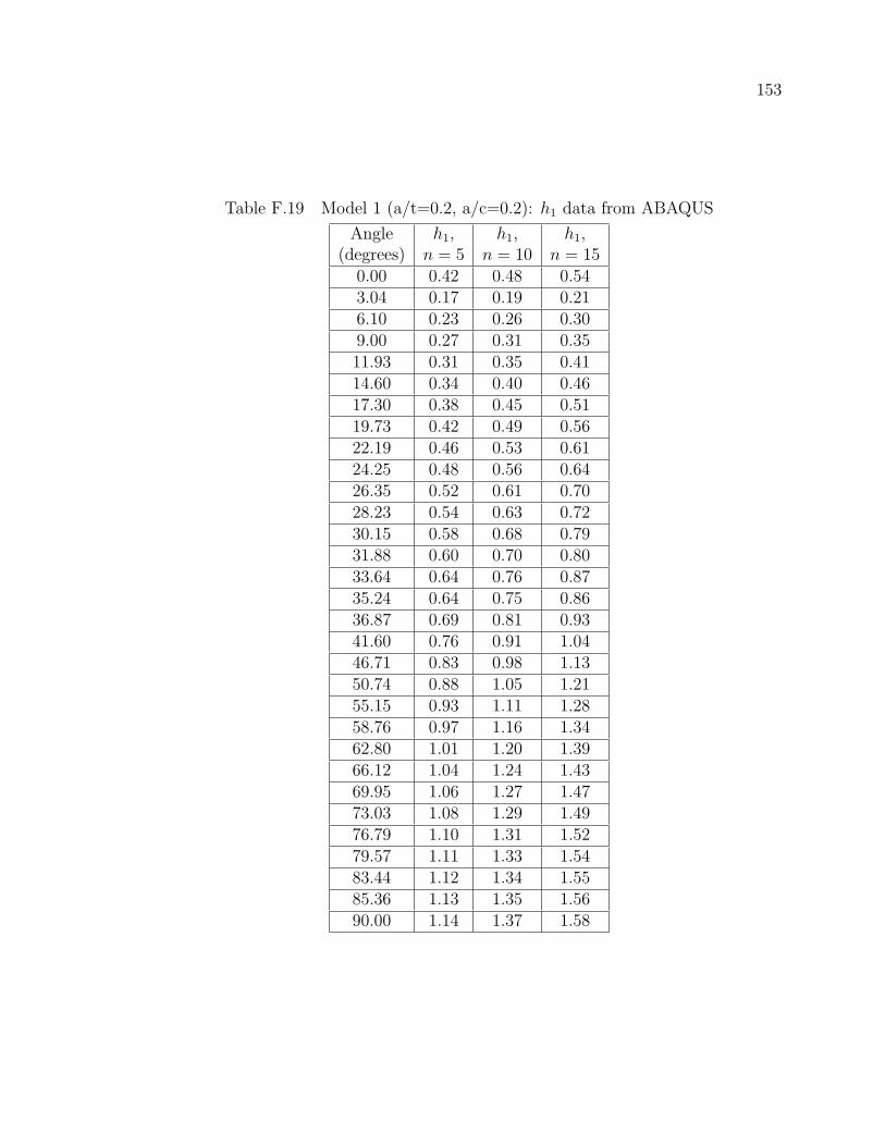
153
Table F.19 Model 1 (a/t=0.2, a/c=0.2): h1 data from ABAQUS
Angle h1, h1, h1,(degrees) n = 5 n = 10 n = 15
0.00 0.42 0.48 0.543.04 0.17 0.19 0.216.10 0.23 0.26 0.309.00 0.27 0.31 0.3511.93 0.31 0.35 0.4114.60 0.34 0.40 0.4617.30 0.38 0.45 0.5119.73 0.42 0.49 0.5622.19 0.46 0.53 0.6124.25 0.48 0.56 0.6426.35 0.52 0.61 0.7028.23 0.54 0.63 0.7230.15 0.58 0.68 0.7931.88 0.60 0.70 0.8033.64 0.64 0.76 0.8735.24 0.64 0.75 0.8636.87 0.69 0.81 0.9341.60 0.76 0.91 1.0446.71 0.83 0.98 1.1350.74 0.88 1.05 1.2155.15 0.93 1.11 1.2858.76 0.97 1.16 1.3462.80 1.01 1.20 1.3966.12 1.04 1.24 1.4369.95 1.06 1.27 1.4773.03 1.08 1.29 1.4976.79 1.10 1.31 1.5279.57 1.11 1.33 1.5483.44 1.12 1.34 1.5585.36 1.13 1.35 1.5690.00 1.14 1.37 1.58

154
Table F.20 Model 2 (a/t=0.2, a/c=0.6): h1 data from ABAQUS
Angle h1, h1, h1,(degrees) n = 5 n = 10 n = 15
0.00 0.63 0.71 0.805.60 0.32 0.33 0.3611.25 0.42 0.47 0.5316.79 0.43 0.48 0.5422.50 0.47 0.54 0.6127.98 0.49 0.57 0.6533.75 0.52 0.61 0.6939.15 0.54 0.63 0.7345.00 0.57 0.67 0.7650.29 0.59 0.69 0.7956.25 0.61 0.72 0.8361.36 0.63 0.74 0.8567.50 0.65 0.77 0.8872.24 0.66 0.78 0.8978.75 0.67 0.80 0.9282.05 0.68 0.80 0.9290.00 0.77 0.92 1.05

155
Table F.21 Model 3 (a/t=0.2, a/c=1.0): h1 data from ABAQUS
Angle h1, h1, h1,(degrees) n = 5 n = 10 n = 15
0.00 0.56 0.66 0.755.60 0.36 0.40 0.4511.25 0.46 0.56 0.6416.79 0.43 0.51 0.5822.50 0.45 0.56 0.6427.98 0.45 0.56 0.6533.75 0.46 0.57 0.6639.15 0.45 0.57 0.6745.00 0.46 0.57 0.6750.29 0.45 0.57 0.6756.25 0.45 0.58 0.6861.36 0.45 0.57 0.6767.50 0.45 0.58 0.6872.24 0.45 0.58 0.6878.75 0.45 0.58 0.6882.05 0.45 0.58 0.6890.00 0.64 0.82 0.96

156
Table F.22 Model 4 (a/t=0.5, a/c=0.2): h1 data from ABAQUS (Part 1)
Angle h1, h1, h1,(degrees) n = 5 n = 10 n = 15
0.00 2.97 5.92 10.033.04 1.44 2.95 5.126.10 1.99 4.22 7.369.00 2.25 4.85 8.5611.93 2.52 5.35 9.3314.60 2.86 6.06 10.6017.30 3.12 6.52 11.2619.73 3.43 7.17 12.3622.19 3.72 7.67 13.1424.25 3.96 8.21 14.0826.35 4.25 8.72 14.8528.23 4.46 9.17 15.6430.15 4.74 9.67 16.4131.88 4.92 10.03 17.0033.64 5.20 10.53 17.7135.24 5.33 10.78 18.1936.87 5.57 11.19 18.7339.40 5.89 11.79 19.6742.02 6.15 12.20 20.2444.32 6.42 12.65 20.9246.71 6.66 13.00 21.3448.83 6.86 13.33 21.8251.06 7.07 13.62 22.1753.05 7.24 13.86 22.5055.15 7.41 14.10 22.7957.05 7.54 14.27 23.0159.05 7.70 14.47 23.2760.87 7.80 14.58 23.3962.80 7.93 14.76 23.6564.55 8.01 14.82 23.6666.42 8.11 14.98 23.9068.12 8.17 15.01 23.8969.95 8.26 15.13 24.08

157
Table F.23 Model 4 (a/t=0.5, a/c=0.2): h1 data from ABAQUS (Part 2)
Angle h1, h1, h1,(degrees) n = 5 n = 10 n = 15
71.60 8.30 15.14 24.0373.40 8.38 15.25 24.2275.00 8.41 15.23 24.1476.79 8.47 15.34 24.3278.34 8.48 15.31 24.2280.13 8.53 15.40 24.3881.62 8.54 15.36 24.2783.44 8.58 15.44 24.4284.81 8.57 15.39 24.3086.72 8.60 15.47 24.4587.68 8.59 15.41 24.3290.00 8.67 15.60 24.65
Table F.24 Model 5 (a/t=0.5, a/c=0.6): h1 data from ABAQUS
Angle h1, h1, h1,(degrees) n = 5 n = 10 n = 15
0.00 2.74 4.43 6.735.60 1.76 2.78 4.1611.25 2.38 4.02 6.2116.79 2.37 4.11 6.4022.50 2.57 4.54 7.1527.98 2.66 4.73 7.4933.75 2.79 4.97 7.8739.15 2.85 5.08 8.0445.00 2.93 5.21 8.2050.29 2.96 5.26 8.2756.25 3.02 5.36 8.4161.36 3.02 5.32 8.3467.50 3.05 5.38 8.4372.24 3.03 5.31 8.3178.75 3.05 5.34 8.3582.05 3.03 5.28 8.2590.00 3.33 5.82 9.07

158
Table F.25 Model 6 (a/t=0.5, a/c=1.0): h1 data from ABAQUS
Angle h1, h1, h1,(degrees) n = 5 n = 10 n = 15
0.00 2.10 3.20 4.685.60 1.60 2.40 3.4611.25 2.06 3.39 5.0516.79 1.94 3.15 4.7522.50 2.01 3.41 5.2327.98 1.99 3.41 5.2833.75 1.98 3.44 5.3539.15 1.95 3.42 5.3545.00 1.93 3.40 5.3150.29 1.89 3.33 5.2056.25 1.86 3.29 5.1561.36 1.82 3.19 4.9767.50 1.80 3.15 4.8972.24 1.76 3.06 4.7378.75 1.75 3.03 4.6882.05 1.73 2.98 4.5890.00 2.23 3.88 5.98
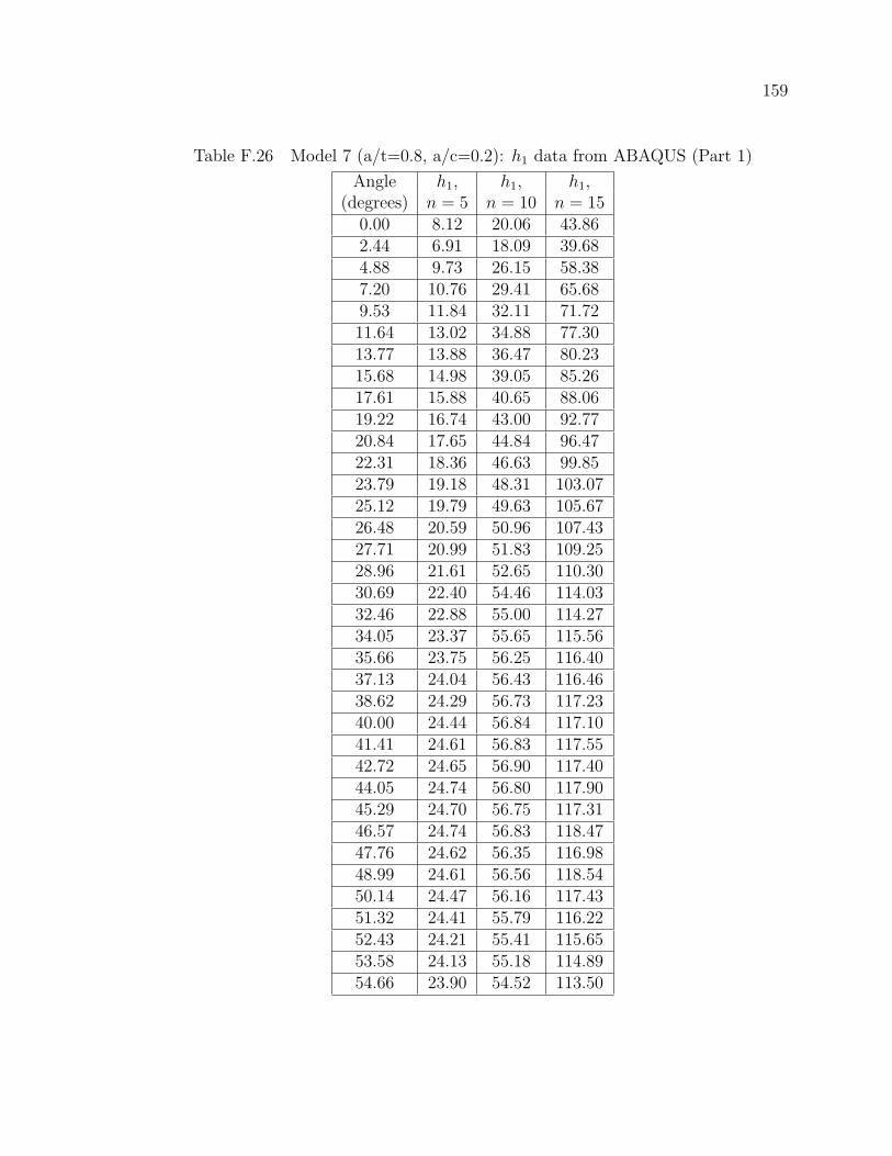
159
Table F.26 Model 7 (a/t=0.8, a/c=0.2): h1 data from ABAQUS (Part 1)
Angle h1, h1, h1,(degrees) n = 5 n = 10 n = 15
0.00 8.12 20.06 43.862.44 6.91 18.09 39.684.88 9.73 26.15 58.387.20 10.76 29.41 65.689.53 11.84 32.11 71.7211.64 13.02 34.88 77.3013.77 13.88 36.47 80.2315.68 14.98 39.05 85.2617.61 15.88 40.65 88.0619.22 16.74 43.00 92.7720.84 17.65 44.84 96.4722.31 18.36 46.63 99.8523.79 19.18 48.31 103.0725.12 19.79 49.63 105.6726.48 20.59 50.96 107.4327.71 20.99 51.83 109.2528.96 21.61 52.65 110.3030.69 22.40 54.46 114.0332.46 22.88 55.00 114.2734.05 23.37 55.65 115.5635.66 23.75 56.25 116.4037.13 24.04 56.43 116.4638.62 24.29 56.73 117.2340.00 24.44 56.84 117.1041.41 24.61 56.83 117.5542.72 24.65 56.90 117.4044.05 24.74 56.80 117.9045.29 24.70 56.75 117.3146.57 24.74 56.83 118.4747.76 24.62 56.35 116.9848.99 24.61 56.56 118.5450.14 24.47 56.16 117.4351.32 24.41 55.79 116.2252.43 24.21 55.41 115.6553.58 24.13 55.18 114.8954.66 23.90 54.52 113.50

160
Table F.27 Model 7 (a/t=0.8, a/c=0.2): h1 data from ABAQUS (Part 2)
Angle h1, h1, h1,(degrees) n = 5 n = 10 n = 15
55.77 23.80 54.35 112.9956.83 23.55 53.55 111.1257.91 23.43 53.35 110.8458.94 23.18 52.65 109.2360.00 23.05 52.42 108.8861.01 22.80 51.82 107.8562.05 22.67 51.72 107.5463.03 22.43 51.18 106.8664.06 22.33 51.16 106.7865.02 22.11 50.81 106.3266.03 22.02 50.81 106.2266.98 21.83 50.45 105.5667.98 21.76 50.52 105.7868.91 21.59 50.15 104.8969.89 21.54 50.25 105.2570.82 21.39 49.85 104.2171.79 21.36 49.97 104.6472.70 21.22 49.54 103.5073.67 21.21 49.66 104.0074.57 21.07 49.20 102.8575.52 21.07 49.33 103.2876.41 20.94 48.86 102.3777.36 20.94 48.99 102.5378.24 20.83 48.57 101.9479.19 20.83 48.73 102.4480.06 20.72 48.28 101.4581.01 20.73 48.48 102.1181.86 20.63 48.07 101.2682.82 20.65 48.26 101.6983.66 20.55 47.92 101.1784.62 20.58 48.12 101.4185.43 20.49 47.80 101.0586.42 20.53 48.04 101.2887.17 20.45 47.73 100.9788.21 20.50 47.99 101.2188.73 20.43 47.70 100.9390.00 20.56 48.15 101.57

161
Table F.28 Model 8 (a/t=0.8, a/c=0.6): h1 data from ABAQUS
Angle h1, h1, h1,(degrees) n = 5 n = 10 n = 15
0.00 5.34 10.81 20.904.03 5.76 12.35 24.448.09 7.63 17.11 34.6411.97 7.51 17.14 35.1215.92 7.94 18.52 38.3319.55 8.07 18.96 39.3223.26 8.13 18.94 39.2726.62 8.17 19.24 39.8530.09 8.18 18.99 39.1033.00 8.12 18.97 39.0736.02 8.17 19.03 38.9938.72 8.03 18.67 38.1741.52 8.05 18.63 37.9644.02 7.86 18.09 36.7746.62 7.89 18.07 36.6548.95 7.60 17.33 35.1651.39 7.55 17.24 35.0554.40 7.41 16.97 34.7057.66 7.18 16.39 33.5160.46 7.04 16.14 33.1863.53 6.94 16.11 33.4466.16 6.83 15.92 33.1169.11 6.79 16.07 33.6771.61 6.72 15.91 33.3074.49 6.72 16.15 33.9576.85 6.66 15.95 33.4779.73 6.68 16.14 33.9081.89 6.63 15.95 33.5384.89 6.66 16.05 33.6486.38 6.61 15.95 33.6090.00 6.87 16.55 34.66

162
Table F.29 Model 9 (a/t=0.8, a/c=1.0): h1 data from ABAQUS
Angle h1, h1, h1,(degrees) n = 5 n = 10 n = 15
0.00 4.13 7.75 14.125.60 4.66 9.48 18.0011.25 5.83 12.63 24.6916.79 5.31 11.71 23.3622.50 5.48 12.58 25.4927.98 5.23 12.09 24.5833.75 5.06 11.65 23.7539.15 4.78 11.01 22.3245.00 4.55 10.31 20.7050.29 4.31 9.68 19.3556.25 4.12 9.26 18.5461.36 3.88 8.76 17.6167.50 3.74 8.44 16.9172.24 3.61 8.29 16.7778.75 3.57 8.29 16.8782.05 3.49 8.11 16.5490.00 3.82 8.87 18.12

APPENDIX G: INCREMENTAL PLASTICITY TABLES
163
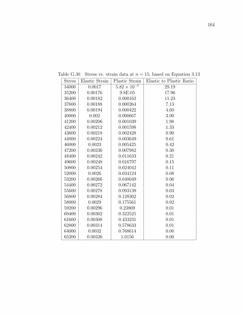
164
Table G.30 Stress vs. strain data at n = 15, based on Equation 3.13
Stress Elastic Strain Plastic Strain Elastic to Plastic Ratio34000 0.0017 5.82× 10⁻⁵ 29.1935200 0.00176 9.8E-05 17.9636400 0.00182 0.000162 11.2337600 0.00188 0.000264 7.1338800 0.00194 0.000422 4.6040000 0.002 0.000667 3.0041200 0.00206 0.001039 1.9842400 0.00212 0.001598 1.3343600 0.00218 0.002428 0.9044800 0.00224 0.003649 0.6146000 0.0023 0.005425 0.4247200 0.00236 0.007982 0.3048400 0.00242 0.011633 0.2149600 0.00248 0.016797 0.1550800 0.00254 0.024042 0.1152000 0.0026 0.034124 0.0853200 0.00266 0.048049 0.0654400 0.00272 0.067142 0.0455600 0.00278 0.093139 0.0356800 0.00284 0.128302 0.0258000 0.0029 0.175561 0.0259200 0.00296 0.23869 0.0160400 0.00302 0.322525 0.0161600 0.00308 0.433231 0.0162800 0.00314 0.578633 0.0164000 0.0032 0.768614 0.0065200 0.00326 1.0156 0.00

165
Table G.31 Stress vs. strain data at n = 10, based on Equation 3.13
Stress Elastic Strain Plastic Strain Elastic to Plastic Ratio30000 0.0015 3.75× 10⁻⁵ 39.9548849335200 0.00176 0.000185667 9.4793204639600 0.00198 0.000602921 3.28401024544000 0.0022 0.001729162 1.27229285548400 0.00242 0.004485 0.5395763752800 0.00264 0.010706513 0.24657887957200 0.00286 0.023837962 0.11997670161600 0.00308 0.050016805 0.06157930366000 0.0033 0.099712174 0.03309525770400 0.00352 0.190123333 0.01851429874800 0.00374 0.348597932 0.01072869279200 0.00396 0.617391497 0.00641408383600 0.00418 1.060160459 0.003942799

166
Table G.32 Stress vs. strain data at n = 5, based on Equation 3.13
Stress Elastic Strain Plastic Strain Elastic to Plastic Ratio22000 0.0011 3.36× 10⁻⁵ 32.7826400 0.00132 8.35× 10⁻⁵ 15.8130000 0.0015 0.000158 9.4835200 0.00176 0.000352 5.0039600 0.00198 0.000634 3.1244000 0.0022 0.001074 2.0548400 0.00242 0.001729 1.4052800 0.00264 0.002672 0.9957200 0.00286 0.003986 0.7261600 0.00308 0.005774 0.5366000 0.0033 0.008153 0.4070400 0.00352 0.011258 0.3174800 0.00374 0.015245 0.2579200 0.00396 0.020288 0.2083600 0.00418 0.026585 0.1688000 0.0044 0.034358 0.1392400 0.00462 0.04385 0.1196800 0.00484 0.055333 0.09101200 0.00506 0.069105 0.07105600 0.00528 0.085493 0.06110000 0.0055 0.104851 0.05114400 0.00572 0.127567 0.04118800 0.00594 0.15406 0.04123200 0.00616 0.184783 0.03127600 0.00638 0.220223 0.03132000 0.0066 0.260903 0.03136400 0.00682 0.307384 0.02140800 0.00704 0.360265 0.02145200 0.00726 0.420186 0.02149600 0.00748 0.487828 0.02154000 0.0077 0.563913 0.01158400 0.00792 0.649209 0.01162800 0.00814 0.744528 0.01167200 0.00836 0.850727 0.01171600 0.00858 0.968713 0.01176000 0.0088 1.099441 0.01

167
Table G.33 Stress vs. plastic strain data at n = 15, used for ABAQUS models
Stress Plastic Strain34000 0.0035200 9.8× 10⁻⁵
36400 0.00016237600 0.00026438800 0.00042240000 0.00066741200 0.00103942400 0.00159843600 0.00242844800 0.00364946000 0.00542547200 0.00798248400 0.01163349600 0.01679750800 0.02404252000 0.03412453200 0.04804954400 0.06714255600 0.09313956800 0.12830258000 0.17556159200 0.2386960400 0.32252561600 0.43323162800 0.57863364000 0.76861465200 1.0156

168
Table G.34 Stress vs. plastic strain data at n = 10, used for ABAQUS models
Stress Plastic Strain30000 0.0035200 0.00018566739600 0.00060292144000 0.00172916248400 0.00448552800 0.01070651357200 0.02383796261600 0.05001680566000 0.09971217470400 0.19012333374800 0.34859793279200 0.61739149783600 1.060160459

169
Table G.35 Stress vs. plastic strain data at n = 5, used for ABAQUS models
Stress Plastic Strain22000 0.0026400 8.35× 10⁻⁵
30000 0.00015835200 0.00035239600 0.00063444000 0.00107448400 0.00172952800 0.00267257200 0.00398661600 0.00577466000 0.00815370400 0.01125874800 0.01524579200 0.02028883600 0.02658588000 0.03435892400 0.0438596800 0.055333101200 0.069105105600 0.085493110000 0.104851114400 0.127567118800 0.15406123200 0.184783127600 0.220223132000 0.260903136400 0.307384140800 0.360265145200 0.420186149600 0.487828154000 0.563913158400 0.649209162800 0.744528167200 0.850727171600 0.968713176000 1.099441

VITA
Eric Quillen was born 1968 in Charlottesville, Virginia. He has an Associates
in General Engineering from Virginia Highlands Community College, a Bachelors of
Science in Manufacturing Engineering Technology from East Tennesse State Univer-
sity. He has been pursuing a masters degree while working full time at Fleetguard,
Inc. He is now a candidate for a Master of Science in Mechanical Engineering.
170