an analysis of four missing data treatment methods for supervised learning
TRANSCRIPT

This article was downloaded by: [University of Maastricht]On: 01 July 2014, At: 17:03Publisher: Taylor & FrancisInforma Ltd Registered in England and Wales Registered Number: 1072954 Registeredoffice: Mortimer House, 37-41 Mortimer Street, London W1T 3JH, UK
Applied Artificial Intelligence: AnInternational JournalPublication details, including instructions for authors andsubscription information:http://www.tandfonline.com/loi/uaai20
An analysis of four missing datatreatment methods for supervisedlearningGustavo E. A. P. A. Batista a & Maria Carolina Monard aa University of Sāo Paulo , Sāo Carlos, SP, BrazilPublished online: 30 Nov 2010.
To cite this article: Gustavo E. A. P. A. Batista & Maria Carolina Monard (2003) An analysis offour missing data treatment methods for supervised learning, Applied Artificial Intelligence: AnInternational Journal, 17:5-6, 519-533, DOI: 10.1080/713827181
To link to this article: http://dx.doi.org/10.1080/713827181
PLEASE SCROLL DOWN FOR ARTICLE
Taylor & Francis makes every effort to ensure the accuracy of all the information (the“Content”) contained in the publications on our platform. However, Taylor & Francis,our agents, and our licensors make no representations or warranties whatsoever as tothe accuracy, completeness, or suitability for any purpose of the Content. Any opinionsand views expressed in this publication are the opinions and views of the authors,and are not the views of or endorsed by Taylor & Francis. The accuracy of the Contentshould not be relied upon and should be independently verified with primary sourcesof information. Taylor and Francis shall not be liable for any losses, actions, claims,proceedings, demands, costs, expenses, damages, and other liabilities whatsoever orhowsoever caused arising directly or indirectly in connection with, in relation to or arisingout of the use of the Content.
This article may be used for research, teaching, and private study purposes. Anysubstantial or systematic reproduction, redistribution, reselling, loan, sub-licensing,systematic supply, or distribution in any form to anyone is expressly forbidden. Terms &Conditions of access and use can be found at http://www.tandfonline.com/page/terms-and-conditions

u AN ANALYSIS OF FOURMISSING DATA TREATMENTMETHODS FOR SUPERVISEDLEARNING
GUSTAVOE. A. P. A. BATISTA andMARIACAROLINAMONARDUniversity of S~ao Paulo, S~ao Carlos, SP, Brazil
One relevant problem in data quality is missing data. Despite the frequent occurrence and the
relevance of the missing data problem, many machine learning algorithms handle missing data
in a rather naive way. However, missing data treatment should be carefully treated, otherwise
bias might be introduced into the knowledge induced. In this work, we analyze the use of the
k-nearest neighbor as an imputation method. Imputation is a term that denotes a procedure
that replaces the missing values in a data set with some plausible values. One advantage of
this approach is that the missing data treatment is independent of the learning algorithm used.
This allows the user to select the most suitable imputation method for each situation. Our
analysis indicates that missing data imputation based on the k-nearest neighbor algorithm can
outperform the internal methods used by C4.5 and CN2 to treat missing data, and can also
outperform the mean or mode imputation method, which is a method broadly used to treat
missing values.
INTRODUCTION
One relevant problem in data quality is missing data. Missing data maybe for different reasons, such as death of patients, equipment malfunctions,refusal of respondents to answer certain questions, and so on. In addition, asignificant fraction of data can be erroneous, and the only alternative may bediscarding the erroneous data.
Data quality is a major concern in machine learning (ML) and othercorrelated areas, such as data mining (DM) and knowledge discovery from
This research is partially supported by Brazilian Research Councils CAPES and FINEP. The authors
would like to thank Andre C.P.L.F. de Carvalho for his suggestions.
Address correspondence to Gustavo E. A. P. A. Batista, Av. do Trabalhador Sao-Carlense, 400, Cx.
Postal 668, Sao Carlos, SP CEP 13560-970, Brazil. E-mail: [email protected]
519
Applied Artificial Intelligence, 17:519–533, 2003
Copyright # 2003 Taylor & Francis
0883-9514/03 $12.00 +.00
DOI: 10.1080/08839510390219309
Dow
nloa
ded
by [
Uni
vers
ity o
f M
aast
rich
t] a
t 17:
03 0
1 Ju
ly 2
014

databases (KDD). Despite the frequent occurrence of missing data in real-world data sets, ML algorithms handle missing data in a rather naive way.Missing data treatment should be carefully treated, otherwise bias might beintroduced into the knowledge induced.
In most cases, data sets attributes are not independent from each other.Thus, through the identification of relationship among attributes, missingvalues can be determined. Imputation is a term that denotes a procedure thatreplaces the missing values in a data set by some plausible values. Oneadvantage of this approach is that the missing data treatment is independentof the learning algorithm used. This allows the user to select the most suitableimputation method for each situation.
The objective of this work is to analyze the performance of the k-nearestneighbor as an imputation method, comparing its performance to three othermissing data treatment methods. The first method is the mean or modeimputation. This method is very simple and broadly used. It consists ofreplacing every missing value of an attribute by the mean (if the attribute isquantitative) or mode (if the attribute is qualitative) of its known values. Theother two methods are the internal missing data treatment strategies used bytwo well known ML algorithms: CN2 (Clark and Niblett 1989) and C4.5(Quinlan 1988).
RANDOMNESS OF MISSING DATA AND METHODS FORTREATING MISSING DATA
Missing data randomness can be divided into three classes as proposed by(Little and Rubin 1987):
1. Missing Completely At Random ðMCARÞ. This is the highest level ofrandomness. It occurs when the probability of an instance (case) having amissing value for an attribute does not depend on either the known valuesor the missing data. In this level of randomness, any missing data treat-ment method can be applied without risk of introducing bias on the data.
2. Missing At Random ðMARÞ. When the probability of an instance having amissing value for an attribute may depend on the known values, but noton the value of the missing data itself.
3. Not Missing At Random ðNMARÞ. When the probability of an instancehaving a missing value for an attribute could depend on the value of thatattribute.
Several methods have been proposed in the literature to treat missingdata. Many of these methods, such as case substitution, were developed fordealing with missing data in sample surveys and have some drawbacks when
520 G. Batista and M. C. Monard
Dow
nloa
ded
by [
Uni
vers
ity o
f M
aast
rich
t] a
t 17:
03 0
1 Ju
ly 2
014
applied to the data mining context. Other methods, such as replacement ofmissing values by the attribute mean or mode, are very naive and should becarefully used to avoid insertion of bias.
In a general way, missing data treatment methods can be divided into thefollowing three categories (Little and Rubin 1987):
1. Ignoring and Discarding Data. There are two main ways to discard datawith missing values. The first one is known as complete case analysis. It isavailable in all statistical packages and is the default method in manyprograms. This method consists of discarding all instances (cases) withmissing data. The second method is known as discarding instances and=orattributes. This method consists of determining the extent of missing dataon each instance and attribute, and deleting the instances and=or attri-butes with high levels of missing data. Before deleting any attribute, it isnecessary to evaluate its relevance to the analysis. Unfortunately, relevantattributes should be kept even with a high degree of missing values. Bothmethods (complete case analysis and discarding instances and=or attributes)should be applied only if missing data are MCAR because missing datathat are not MCAR have non-random elements that can bias the results.
2. Parameter Estimation. Maximum likelihood procedures are used to esti-mate the parameters of a model defined for the complete data. Maximumlikelihood procedures that use variants of the expectation-maximizationalgorithm (Dempster et al. 1977) can handle parameter estimation in thepresence of missing data.
3. Imputation. Imputation is a class of procedures that aims to fill in themissing values with estimated ones. The objective is to employ knownrelationships that can be identified in the valid values of the data set toassist in estimating the missing values. This paper focuses on imputation ofmissing data. More details about this class of methods are described next.
IMPUTATION METHODS
Imputation methods involve replacing missing values with estimated onesbased on information available in the data set. There are many optionsvarying from naive methods, such as mean imputation, to some more robustmethods based on relationships among attributes. A description of somewidely used imputation methods follows:
1. Case Substitution. This method is typically used in sample surveys. Oneinstance with missing data (for example, a person that cannot becontacted) is replaced by another non-sampled instance.
2. Mean or Mode Imputation. This is one of the most frequently usedmethods. It consists of replacing the missing data for a given attribute by
Missing Data Treatment Methods 521
Dow
nloa
ded
by [
Uni
vers
ity o
f M
aast
rich
t] a
t 17:
03 0
1 Ju
ly 2
014

the mean (quantitative attribute) or mode (qualitative attribute) of allknown values of that attribute.
3. Hot Deck and Cold Deck. In the hot deck method, a missing attributevalue is filled in with a value from an estimated distributation for themissing value from the current data. Hot deck is typically implemented intwo stages. In the first stage, the data are partitioned into clusters. In thesecond stage, each instance with missing data is associated with onecluster. The complete cases in a cluster are used to fill in the missingvalues. This can be done by calculating the mean or mode of the attributewithin a cluster. Cold deck imputation is similar to hot deck, but the datasource must be other than the current data source.
4. Prediction Model. Prediction models are sophisticated procedures forhandling missing data. These methods consist of creating a predictivemodel to estimate values that will substitute the missing data. The attri-bute with missing data is used as class-attribute, and the remainingattributes are used as input for the predictive model. An importantargument in favor of this approach is that, frequently, attributes haverelationships (correlations) among themselves. In this way, those corre-lations could be used to create a predictive model for classification orregression for, respectively, qualitative and quantitative attributes withmissing data. Some of these relationships among the attributes may bemaintained if they are captured by the predictive model. An importantdrawback of this approach is that the model estimated values are usuallymore well-behaved than the true values would be, i.e., since the missingvalues are predicted from a set of attributes, the predicted values are likelyto be more consistent with this set of attributes than the true (not known)values would be. A second drawback is the requirement for correlationamong the attributes. If there are no relationships among attributes in thedata set and the attribute with missing data, then the model will not beprecise for estimating missing values.
IMPUTATION WITH k-NEAREST NEIGHBOR
This work proposes the use of the k-nearest neighbor algorithm to esti-mate and substitute missing data. The main benefits of this approach are:(i) k-nearest neighbor can predict both qualitative attributes (the most fre-quent value among the k-nearest neighbors) and quantitative attributes (themean among the k-nearest neighbors); (ii) there is no necessity for creating apredictive model for each attribute with missing data. Actually, the k-nearestneighbor algorithm does not create explicit models (such as a decision tree ora set of rules), since the data set is used as a ‘‘lazy’’ model. Thus, the k-nearest
522 G. Batista and M. C. Monard
Dow
nloa
ded
by [
Uni
vers
ity o
f M
aast
rich
t] a
t 17:
03 0
1 Ju
ly 2
014

neighbor algorithm can be easily adapted to work with any attribute as classby just modifying the attributes to be considered in the distance metric. Also,this approach can easily treat examples with multiple missing values.
The main drawback of the k-nearest neighbor approach is that, wheneverthe k-nearest neighbor looks for the most similar instances, the algorithmsearches through all the data sets. This limitation can be very critical forKDD, since this research area has, as one of its main objectives, the analysisof large databases. Several works that aim to solve this limitation can befound in the literature. One method is the creation of a reduced training setfor the k-nearest neighbor composed only by proto-typical examples (Wilsonand Martinez 2000). This work uses an access method called M-tree (Ciacciaet al. 1997) that was implemented in the k-nearest neighbor algorithmemployed. Furthermore, M-trees can organize and search data sets based ona generic metric space. M-trees can drastically reduce the number of distancecomputations in similarity queries.
MISSING DATA TREATMENT BY C4.5 AND CN2
Both algorithms, C4.5 and CN2, were selected because they are wellconsidered by the ML community. They induce propositional concepts:decision trees and rules, respectively. Furthermore, C4.5 seems to have agood internal algorithm to treat missing values, as shown in Grzymala-Busseand Hu (2000). On the other hand, CN2 seems to use a rather simple methodto treat missing data.
C4.5 and CN2 can handle missing values in any attribute, except the classattribute, for both training and test sets.
C4.5 uses a probabilistic approach to handle missing data. Given atraining set, T, C4.5 finds a suitable test, based on a single attribute, that hasone or more mutually exclusive outcomes O1;O2; . . . ;On. T is partitioned intosubsets T1;T2; . . . ; Tn, where Ti contains all the instances in T that satisfy thetest with outcome Oi. The same algorithm is applied to each subset Ti until astop criteria is obeyed. C4.5 uses the information gain ratio measure to choosea good test to partition the instances. If there exist missing values in anattribute X, C4.5 uses the subset with all known values to X to calculate theinformation gain.
Once a test based on an attribute X is chosen, C4.5 uses a probabilisticapproach to partition the instances with missing values in X. When aninstance in T with known value is assigned to a subset Ti, this indicates thatthe probability of that instance belonging to subset Ti is 1 and to all othersubsets is 0. When the value is not known, only a weaker probabilisticstatement can be made. C4.5 associates to each instance in Ti a weightrepresenting the probability of that instance belonging to Ti. If the instancehas a known value and satisfies the test with outcome Oi, then this instance is
Missing Data Treatment Methods 523
Dow
nloa
ded
by [
Uni
vers
ity o
f M
aast
rich
t] a
t 17:
03 0
1 Ju
ly 2
014

assigned to Ti with weight 1; if the instance has an unknown value, thisinstance is assigned to all partitions with different weights for each one. Theweight for the partition Ti is the probability that instance belongs to Ti. Thisprobability is estimated as the sum of the weights of insances in T known tosatisfy the test with outcome Oi divided by the sum of weights of the cases inT with known values on the attributes X.
The CN2 algorithm uses a rather simple imputation method to treatmissing data. Every missing value is filled in with its attribute most commonknown value before calculating the entropy measure (Clark and Niblett1989).
EXPERIMENTAL ANALYSIS
The main objective of the experiments conducted in this work is toevaluate the efficiency of the k-nearest neighbor algorithm as an imputationmethod to treat missing data, comparing its performance with the perfor-mance obtained by the internal algorithms used by C4.5 and CN2 to learnwith missing data and by the mean or mode imputation method.
In these experiments, missing values were artificially implanted in diffe-rent rates and attributes into the data sets. The performance of all fourmissing data treatments were compared using cross-validation estimatederror rates. In particular, we are interested in analyzing the behavior of thesetreatments when the amount of missing data is high since some researchershave reported finding databases where more than 50% of the data weremissing (Lakshminarayan et al. 1999).
The experiments were carried using four data sets from UCI (Merz andMurphy 1998) Bupa, Cmc, Pima, and Breast. The first three data sets have nomissing values. Breast has very few cases with missing values (in total sixteencases or 2.28%), which were removed before starting the experiments. Themain reason for not using data with missing values is the wish to have totalcontrol over the missing data in the data set. For instance, we would like thetest sets to have no missing data. If some test set has missing data, then theinducer’s ability to classify missing data properly may influence the result.This influence is undesirable since the objective of this work is to analyze theviability of the k-nearest neighbor as an imputation method for missing dataand the inducer learning ability when missing values are present.
Table 1 summarizes the data sets employed in this study. It shows, foreach data set, the number of instances (#Instances), number and percentageof duplicate (appearing more than once) or conflicting (same attribute-valuebut different class attribute) instances, number of attributes (#Attributes),number of quantitative and qualitative attributes, class attribute distribution,and the majority class error. This information was obtained using theMLCþþ info utility (Kohavi et al. 1996).
524 G. Batista and M. C. Monard
Dow
nloa
ded
by [
Uni
vers
ity o
f M
aast
rich
t] a
t 17:
03 0
1 Ju
ly 2
014

Initially, the original data set was partitioned into ten pairs of trainingand test sets through the application of ten-fold cross validation resamplingmethod. Then, missing values were inserted into the training set. Six copies ofthis training set were used; two were given directly to C4.5 and CN2 withoutany missing data treatment. Another two copies had their missing valuestreated, by the mean or mode imputation method and the last two copieswere given to the k-nearest neighbor to estimate and substitute the missingvalues. After the missing data treatment, the training sets were given to C4.5and CN2. All classifiers, i.e., the two induced with untreated data andthe other four induced with treated data, were used to classify the test set. Atthe end of ten iterations, the true error rate was estimated by calculating themean of the error rates of each iteration. Finally, the performances of C4.5and CN2 allied to the k-nearest neighbor missing data treatment methodwere analyzed and compared to the performances of the methods usedinternally by C4.5 and CN2 to learn when missing values are present, and tothe performances of C4.5 and CN2 allied to the mean or mode imputation.
In order to insert missing data into the training sets, some attributes haveto be chosen and some of their values modified to unknown. Which attributeswill be chosen and how many of their values will be modified to unknown isan important decision. It is straightforward to see that the most repre-sentative attributes of the data set are a sensible choice for the attributes thatshould have their values modified to unknown. Otherwise, the analysis maybe compromised by treating non-representative attributes that will not beincorporated into the classifier by the learning system. Since finding the mostrepresentative attributes of a data set is not a trivial task, we used the resultsof Lee et al. (1999) to select the three most relevant attributes according toseveral feature subset selection methods, such as wrapper and filter.
Related to the amount of missing data to be inserted into the trainingsets, we want to analyze the behavior of the methods with different amounts
TABLE 1 Data Sets Summary Descriptions
Data set #Instances
#Duplicate or
conflicting (%)
#Attributes
(quanti., quali.) Class Class%
Majority
Error
bupa 345 4 (1.16%) 6 (6,0) 1 42.03 42.03%
2 57.97 on value 2
cmc 1473 115 (7.81%) 9 (2,7) 1 42.70 57.30%
2 22.61 on value 1
3 34.69
pima 769 1 (0.13%) 8 (8,0) 0 65.02 34.98%
1 34.98 on value 0
breast 699 8 (1.15%) 9 (9,0) 2 65.52 34.48%
4 34.48 on value 2
Missing Data Treatment Methods 525
Dow
nloa
ded
by [
Uni
vers
ity o
f M
aast
rich
t] a
t 17:
03 0
1 Ju
ly 2
014
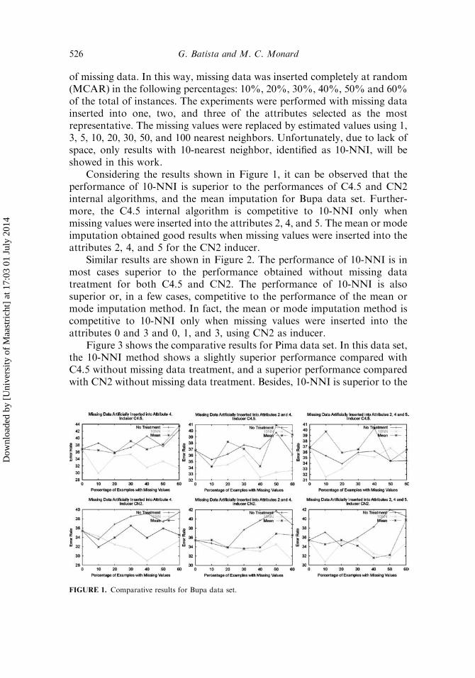
of missing data. In this way, missing data was inserted completely at random(MCAR) in the following percentages: 10%, 20%, 30%, 40%, 50% and 60%of the total of instances. The experiments were performed with missing datainserted into one, two, and three of the attributes selected as the mostrepresentative. The missing values were replaced by estimated values using 1,3, 5, 10, 20, 30, 50, and 100 nearest neighbors. Unfortunately, due to lack ofspace, only results with 10-nearest neighbor, identified as 10-NNI, will beshowed in this work.
Considering the results shown in Figure 1, it can be observed that theperformance of 10-NNI is superior to the performances of C4.5 and CN2internal algorithms, and the mean imputation for Bupa data set. Further-more, the C4.5 internal algorithm is competitive to 10-NNI only whenmissing values were inserted into the attributes 2, 4, and 5. The mean or modeimputation obtained good results when missing values were inserted into theattributes 2, 4, and 5 for the CN2 inducer.
Similar results are shown in Figure 2. The performance of 10-NNI is inmost cases superior to the performance obtained without missing datatreatment for both C4.5 and CN2. The performance of 10-NNI is alsosuperior or, in a few cases, competitive to the performance of the mean ormode imputation method. In fact, the mean or mode imputation method iscompetitive to 10-NNI only when missing values were inserted into theattributes 0 and 3 and 0, 1, and 3, using CN2 as inducer.
Figure 3 shows the comparative results for Pima data set. In this data set,the 10-NNI method shows a slightly superior performance compared withC4.5 without missing data treatment, and a superior performance comparedwith CN2 without missing data treatment. Besides, 10-NNI is superior to the
FIGURE 1. Comparative results for Bupa data set.
526 G. Batista and M. C. Monard
Dow
nloa
ded
by [
Uni
vers
ity o
f M
aast
rich
t] a
t 17:
03 0
1 Ju
ly 2
014

mean or mode imputation when missing data were inserted into attribute 1for both inducers.With missing data inserted into more than one attribute, 10-NNI and meanor mode imputation show similar results.
Table 2 shows some numerical results related to the graphs presented inFigures 1, 2, and 3. This table shows the error rates and standard deviations.More detailed results can be found in Batista and Monard (2002).
It is important to say that, for Bupa, Cmc, and Pima data sets, theinternal methods used by C4.5 and CN2 to treat missing data show lower
FIGURE 2. Comparative results for Cmc data set.
FIGURE 3. Comparative results for Pima data set.
Missing Data Treatment Methods 527
Dow
nloa
ded
by [
Uni
vers
ity o
f M
aast
rich
t] a
t 17:
03 0
1 Ju
ly 2
014

TABLE 2 Comparative Results for Bupa, Cmc, Pima, and Breast Data Sets
C4.5 CN2
Data
set Attr. %
No
Imputation Mean=Mode 10-NNI
No
Imputation Mean=Mode 10-NNI
0 36.82±2.69 – – 35.39±2.47 – –
10 38.56±1.74 36.50±1.76 29.87±1.76 33.58±1.94 31.91±1.88 34.19±1.45
20 35.95±1.24 35.66±1.61 34.78±2.43 36.82±0.96 33.95±1.70 32.45±0.95
4 30 37.36±1.89 39.14±2.41 35.36±2.71 38.53±2.16 36.52±1.74 31.56±2.71
40 40.56±2.05 36.78±1.72 31.55±1.86 39.13±1.09 33.91±1.36 28.96±2.24
50 37.62±2.35 38.22±3.03 33.34±2.54 37.35±2.74 35.92±2.09 31.28±1.91
60 42.31±2.11 43.45±2.08 31.22±3.33 39.41±1.20 34.51±2.78 33.29±2.64
0 36.82±2.69 – – 35.39±2.47 – –
10 35.32±2.36 34.20±2.23 34.18±1.72 34.75±2.01 35.45±2.21 33.63±1.77
20 36.22±2.18 38.21±2.54 34.51±2.16 33.81±3.23 33.89±1.49 31.81±2.65
Bupa 4, 2 30 37.70±2.40 37.07±2.44 35.96±2.05 37.66±1.48 33.61±1.96 33.34±1.88
40 37.08±1.42 34.25±1.76 32.45±1.09 39.67±1.98 33.88±1.27 33.02±2.44
50 39.71±2.76 40.89±2.31 33.28±3.07 41.72±1.38 36.83±1.88 34.51±2.40
60 36.21±1.84 39.36±2.30 33.57±2.38 38.81±1.58 36.51±2.33 31.01±1.48
0 36.82±2.69 – – 35.39±2.47 – –
10 35.36±1.76 39.71±1.91 31.56±2.44 37.09±2.55 34.50±1.81 30.71±2.47
20 33.92±2.07 35.92±1.17 33.05±2.09 34.18±2.03 35.39±1.75 34.81±1.49
4, 2, 5 30 35.97±2.90 36.52±1.68 35.61±3.00 35.94±2.14 34.18±1.92 35.35±1.39
40 36.19±2.39 40.29±2.47 35.11±2.14 38.25±1.49 31.59±2.51 32.49±1.20
50 34.39±2.84 34.45±1.75 36.75±2.12 41.97±1.58 32.18±2.24 31.56±1.58
60 34.48±1.77 36.46±1.71 34.47±3.02 40.56±1.88 39.72±1.63 34.82±2.04
0 48.27±0.83 – – 51.25±0.80 – –
10 49.35±1.14 50.24±1.15 48.20±1.16 51.19±1.51 49.69±1.34 50.64±1.22
20 50.23±1.12 49.35±0.85 47.59±0.98 51.73±1.17 49.15±1.42 49.08±0.95
3 30 49.49±0.95 50.78±1.45 47.39±1.48 52.27±0.94 52.21±1.13 49.70±1.71
40 49.97±0.87 48.54±1.46 48.54±1.12 53.56±1.47 51.60±0.73 50.51±1.11
50 50.71±1.11 50.51±1.15 49.36±0.91 54.92±0.95 51.39±1.39 49.56±1.74
60 52.88±1.25 49.90±1.07 47.73±0.95 54.24±1.31 51.93±1.50 50.51±1.12
0 48.27±0.83 – – 51.25±0.80 – –
10 48.27±0.67 48.27±1.37 47.32±1.30 51.26±0.80 49.83±0.77 48.75±1.42
20 48.27±0.99 49.62±1.42 48.61±1.30 52.48±1.51 50.78±1.20 48.88±1.46
Cmc 3, 0 30 48.88±1.40 50.58±0.98 49.02±1.36 52.68±0.91 50.92±0.95 48.54±1.34
40 48.61±1.20 49.56±1.33 47.59±1.53 52.35±1.10 50.11±1.43 50.44±1.09
50 49.49±0.84 49.15±1.38 46.23±1.06 52.68±0.81 48.68±1.18 50.03±1.76
60 50.64±1.16 50.24±0.91 47.39±1.87 51.12±1.53 50.10±1.38 50.85±1.49
0 48.27±0.83 – – 51.25±0.80 – –
10 46.78±1.46 47.32±0.78 47.18±1.19 51.32±1.19 49.56±1.46 49.70±1.61
20 49.56±1.34 51.40±1.49 48.34±1.29 52.14±1.04 51.12±1.07 51.66±1.06
3, 0, 1 30 48.20±1.19 51.18±0.89 48.13±1.51 52.95±1.25 52.34±1.45 51.46±1.15
40 51.26±1.33 48.54±1.12 47.45±1.46 53.36±1.23 49.83±0.85 50.10±1.49
50 50.31±1.23 50.84±1.61 47.38±1.74 52.68±1.02 51.94±1.29 51.73±1.82
60 52.75±1.16 51.46±1.06 48.75±1.86 52.88±0.76 52.75±1.05 50.92±1.35
(Continued)
528 G. Batista and M. C. Monard
Dow
nloa
ded
by [
Uni
vers
ity o
f M
aast
rich
t] a
t 17:
03 0
1 Ju
ly 2
014

TABLE 2 Continued.
C4.5 CN2
Data
set Attr. %
No
Imputation Mean=Mode 10-NNI
No
Imputation Mean=Mode 10-NNI
0 26.56±1.16 – – 25.77±1.12 – –
10 26.17±1.03 26.42±1.48 24.86±0.88 27.99±0.98 28.38±0.87 25.91±0.86
20 28.65±1.15 26.68±1.18 26.04±1.68 28.51±1.06 28.76±1.51 26.18±0.78
1 30 28.25±1.85 27.59±1.38 27.35±1.03 27.47±1.11 29.30±1.23 26.69±1.61
40 26.95±1.67 28.90±1.23 25.38±1.15 30.21±1.08 30.34±1.59 26.82±0.98
50 28.11±1.14 27.86±0.84 26.17±1.11 30.34±1.21 29.68±1.58 27.35±1.47
60 30.59±1.13 27.34±1.05 26.29±1.90 30.21±1.28 30.72±1.47 25.78±1.33
0 26.56±1.16 – – 25.77±1.12 – –
10 25.25±1.10 26.56±1.08 27.86±1.15 28.38±0.87 26.69±1.31 27.08±0.98
20 26.94±1.22 25.91±1.34 26.43±1.08 28.76±1.51 23.43±0.68 28.25±1.09
Pima 1, 5 30 27.73±1.60 26.42±1.27 25.39±0.81 29.30±1.23 27.86±1.16 25.65±1.13
40 27.21±1.45 28.12±1.11 26.29±1.69 30.34±1.59 26.57±1.73 26.17±1.07
50 25.78±1.13 27.99±1.37 27.46±1.16 29.68±1.58 26.17±0.82 25.91±1.08
60 29.81±1.43 27.46±1.67 27.85±1.51 30.72±1.47 27.47±0.75 27.60±1.47
0 26.56±1.16 – – 25.77±1.12 – –
10 25.11±1.70 25.51±1.90 25.13±0.90 27.48±1.00 28.38±0.99 27.73±0.68
20 26.30±1.01 27.33±1.42 25.65±1.35 29.82±0.82 26.30±1.13 27.87±1.26
1, 5, 0 30 26.17±1.35 27.48±1.19 25.51±1.75 31.25±0.89 27.73±0.91 26.17±1.32
40 26.82±1.28 25.65±0.84 25.91±1.44 29.03±0.90 27.35±0.92 25.92±1.32
50 28.11±1.32 28.11±1.65 24.61±1.16 29.69±0.41 26.83±1.29 25.26±0.68
60 27.60±1.05 27.34±1.53 27.86±1.55 31.51±1.17 23.83±0.95 26.05±0.86
0 4.24±0.67 – – 4.68±0.60 – –
10 3.80±0.93 3.66±0.82 4.25±0.67 4.39±0.44 4.24±0.46 5.12±0.84
20 3.95±0.90 3.51±0.88 5.11±0.99 4.68±0.75 4.83±0.69 4.39±0.57
1 30 3.95±0.90 3.80±0.93 4.09±0.91 4.97±0.82 4.67±1.03 4.97±0.62
40 3.95±0.90 3.95±0.90 4.53±0.82 4.53±0.73 5.12±0.90 4.53±0.70
50 3.95±0.90 3.95±0.90 5.41±1.00 4.53±0.91 4.82±0.87 4.53±0.63
60 3.95±0.90 3.95±0.90 6.00±0.88 4.83±0.84 4.83±1.07 5.12±0.69
0 4.24±0.67 – – 4.68±0.60 – –
10 4.83±0.61 3.80±0.85 4.10±0.61 4.38±0.65 3.80±0.66 4.38±0.75
20 4.97±0.65 4.68±0.64 3.80±0.88 3.65±0.84 4.53±0.67 5.56±0.77
Breast 1, 5 30 4.68±0.61 4.39±0.65 4.83±0.69 3.95±0.54 4.09±0.97 4.69±0.57
40 4.39±0.65 4.97±0.44 4.98±0.54 3.95±0.87 3.51±0.66 4.96±0.99
50 4.98±0.73 4.69±0.37 3.81±0.63 4.53±0.63 4.68±0.75 4.98±0.76
60 4.54±0.71 4.68±0.65 5.85±0.53 4.39±0.95 3.66±0.66 4.25±0.64
0 4.24±0.67 – – 4.68±0.60 – –
10 4.68±0.75 4.10±0.61 4.83±0.81 4.25±0.71 4.10±0.52 4.83±0.76
20 5.12±0.73 4.83±0.69 4.69±0.68 4.97±0.79 4.39±0.66 3.80±0.62
1, 5, 0 30 5.42±0.69 4.98±0.50 4.69±1.02 5.12±0.54 5.41±0.78 4.24±0.80
40 4.97±0.62 4.09±0.68 5.27±0.85 5.13±0.55 3.65±0.82 4.83±0.62
50 5.41±0.57 4.83±0.61 4.10±0.84 5.85±0.76 3.07±0.82 4.24±0.91
60 4.97±0.73 4.68±0.78 4.68±0.80 5.85±0.61 3.80±0.73 5.11±0.97
Missing Data Treatment Methods 529
Dow
nloa
ded
by [
Uni
vers
ity o
f M
aast
rich
t] a
t 17:
03 0
1 Ju
ly 2
014
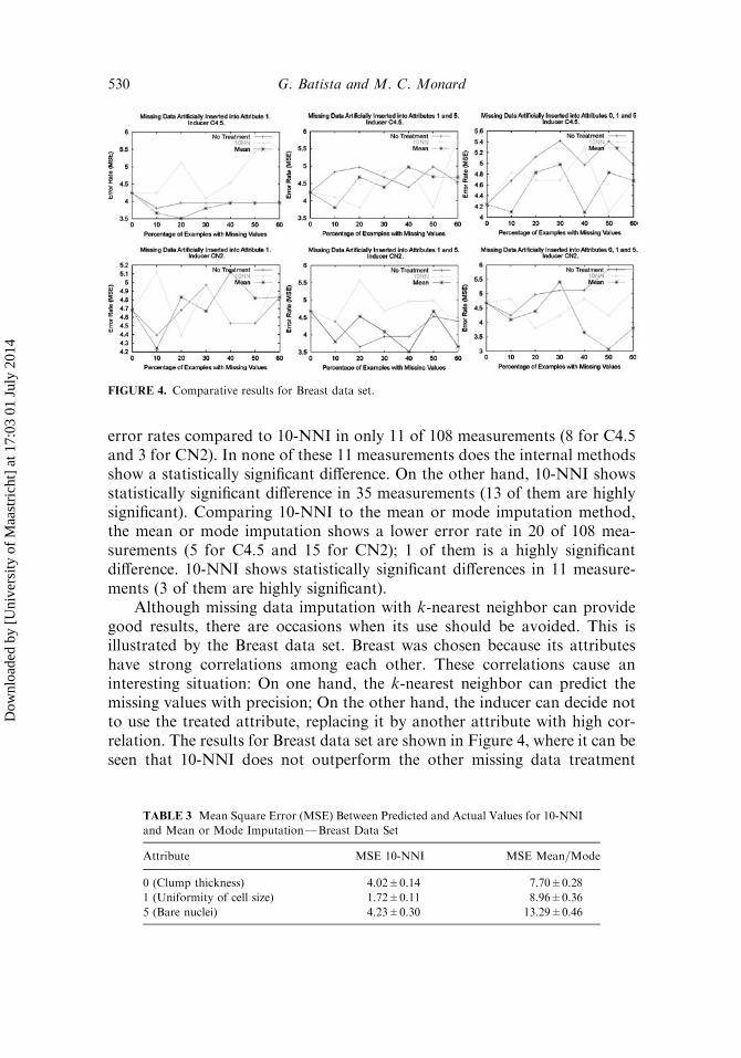
error rates compared to 10-NNI in only 11 of 108 measurements (8 for C4.5and 3 for CN2). In none of these 11 measurements does the internal methodsshow a statistically significant difference. On the other hand, 10-NNI showsstatistically significant difference in 35 measurements (13 of them are highlysignificant). Comparing 10-NNI to the mean or mode imputation method,the mean or mode imputation shows a lower error rate in 20 of 108 mea-surements (5 for C4.5 and 15 for CN2); 1 of them is a highly significantdifference. 10-NNI shows statistically significant differences in 11 measure-ments (3 of them are highly significant).
Although missing data imputation with k-nearest neighbor can providegood results, there are occasions when its use should be avoided. This isillustrated by the Breast data set. Breast was chosen because its attributeshave strong correlations among each other. These correlations cause aninteresting situation: On one hand, the k-nearest neighbor can predict themissing values with precision; On the other hand, the inducer can decide notto use the treated attribute, replacing it by another attribute with high cor-relation. The results for Breast data set are shown in Figure 4, where it can beseen that 10-NNI does not outperform the other missing data treatment
TABLE 3 Mean Square Error (MSE) Between Predicted and Actual Values for 10-NNI
and Mean or Mode Imputation—Breast Data Set
Attribute MSE 10-NNI MSE Mean=Mode
0 (Clump thickness) 4.02±0.14 7.70±0.28
1 (Uniformity of cell size) 1.72±0.11 8.96±0.36
5 (Bare nuclei) 4.23±0.30 13.29±0.46
FIGURE 4. Comparative results for Breast data set.
530 G. Batista and M. C. Monard
Dow
nloa
ded
by [
Uni
vers
ity o
f M
aast
rich
t] a
t 17:
03 0
1 Ju
ly 2
014
methods. This scenario is interesting because 10-NNI was able to predict themissing data with higher precision than the mean or mode imputation. Asmissing values were artificially implanted into the data, the mean square error(MSE) between the predicted values and the actual ones can be measured.These errors are presented in Table 3.
If 10-NNI method was more accurate in predicting the missing values,why does this higher accuracy not translate into a more precise classifier? Theanswer may be in the high correlation among the data set attributes andbecause (or consequently) Breast data set has several attributes with similarpredicting power.
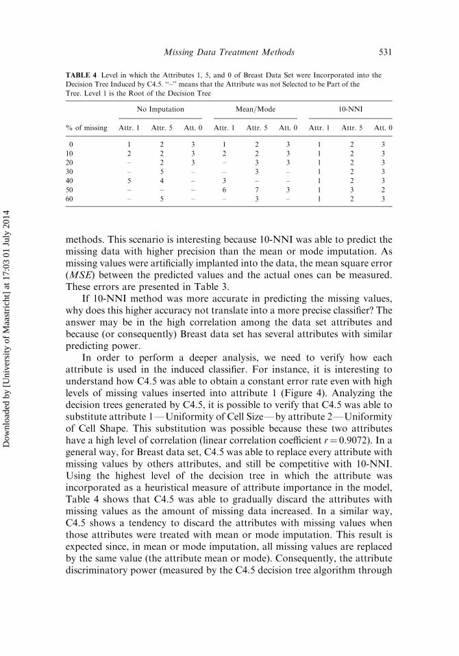
In order to perform a deeper analysis, we need to verify how eachattribute is used in the induced classifier. For instance, it is interesting tounderstand how C4.5 was able to obtain a constant error rate even with highlevels of missing values inserted into attribute 1 (Figure 4). Analyzing thedecision trees generated by C4.5, it is possible to verify that C4.5 was able tosubstitute attribute 1—Uniformity of Cell Size—by attribute 2—Uniformityof Cell Shape. This substitution was possible because these two attributeshave a high level of correlation (linear correlation coefficient r¼ 0.9072). In ageneral way, for Breast data set, C4.5 was able to replace every attribute withmissing values by others attributes, and still be competitive with 10-NNI.Using the highest level of the decision tree in which the attribute wasincorporated as a heuristical measure of attribute importance in the model,Table 4 shows that C4.5 was able to gradually discard the attributes withmissing values as the amount of missing data increased. In a similar way,C4.5 shows a tendency to discard the attributes with missing values whenthose attributes were treated with mean or mode imputation. This result isexpected since, in mean or mode imputation, all missing values are replacedby the same value (the attribute mean or mode). Consequently, the attributediscriminatory power (measured by the C4.5 decision tree algorithm through
TABLE 4 Level in which the Attributes 1, 5, and 0 of Breast Data Set were Incorporated into the
Decision Tree Induced by C4.5. ‘‘–’’ means that the Attribute was not Selected to be Part of the
Tree. Level 1 is the Root of the Decision Tree
No Imputation Mean=Mode 10-NNI
% of missing Attr. 1 Attr. 5 Att. 0 Attr. 1 Attr. 5 Att. 0 Attr. 1 Attr. 5 Att. 0
0 1 2 3 1 2 3 1 2 3
10 2 2 3 2 2 3 1 2 3
20 – 2 3 – 3 3 1 2 3
30 – 5 – – 3 – 1 2 3
40 5 4 – 3 – – 1 2 3
50 – – – 6 7 3 1 3 2
60 – 5 – – 3 – 1 2 3
Missing Data Treatment Methods 531
Dow
nloa
ded
by [
Uni
vers
ity o
f M
aast
rich
t] a
t 17:
03 0
1 Ju
ly 2
014

entropy) tends to decrease. The same did not occur when the missing datawere treated by 10-NNI. In this scenario, C4.5 kept the attributes withmissing values as the upmost attributes into the decision tree. This situationwould have been an advantage if Breast data set did not have other attributeswith similar predicting power.
CONCLUSIONS AND LIMITATIONS
This work analyzes the behavior of four methods for missing datatreatment: the 10-NNI method using a k-nearest neighbor algorithm formissing data imputation; the mean or mode imputation; and the internalalgorithms used by C4.5 and CN2 to treat missing data. These methods wereanalyzed inserting different percentages of missing data into differentattributes of four data sets showing promising results. The 10-NNI providesvery good results, even for training sets having a large amount of missingdata.
The Breast data set provided a valuable insight into the limitations of themissing data treatment methods. The first decision to be made is if theattribute should be treated. The existence of other attributes with similarinformation (high correlation), or similar predicting power can make themissing data imputation useless or even harmful. Missing data imputationcan be harmful because even the most advanced imputation method is onlyable to approximate the actual (missing) value. The predicted values areusually more well-behaved, since they conform with other attributes values.In the experiments carried out, as more attributes with missing values wereinserted and as the amount of missing data increased, the induced modelsbecame more simple. In this way, missing data imputation should becarefully applied under the risk of oversimplifying the problem under study.
In future works, the missing data treatment methods will be analyzed inother data sets. Furthermore, in this work, missing values were insertedcompletely at random (MCAR). In a future work, we will analyze thebehavior of these methods when missing values are not randomly distributed.In this case, there is a possibility of creating invalid knowledge. For aneffective analysis, we will have to inspect not only the error rate, but also thequality of the knowledge induced by the learning system.
REFERENCES
Batista, G. E., and M. C. Monard. 2003. Experimental comparison of k-nearest neighbour and mean or
mode imputation methods with the internal strategies used by C4.5 and CN2 to treat missing data.
Technical Report 186, ICMC USP.
Ciaccia, P., M. Patella, and P. Zezula. 1997. M-tree: An efficient access method for similarity search in
metric spaces. In Proceedings of the 23rd VLDB International Conference, pages 426–435, September
1997, Athens, Greece.
532 G. Batista and M. C. Monard
Dow
nloa
ded
by [
Uni
vers
ity o
f M
aast
rich
t] a
t 17:
03 0
1 Ju
ly 2
014

Clark, P. and T. Niblett. 1989. The CN2 induction algorithm. Machine Learning 3(4):261–283.
Dempster, A. P., N. M. Laird, and D. B. Rubin. 1977. Maximum likelihood from incomplete data via the
EM algorithm (with discussion). Journal of Royal Statistical Society B39:1–38.
Grzymala-Busse, J. W., and M. Hu. 2000. A comparison of several approaches to missing attribute values
in data mining. In Proceedings of the Second International Conference on Rough Sets and Current
Trends in Computing (RSCTC 2000), pages 378–385, October 16–19, 2000, Banff, Canada.
Kohavi, R., D. Sommerfield, and J. Dougherty. 1997. Data mining using MLCþþ : A machine learning
library in Cþþ . International Journal on Artificial Intelligence Tools 6(4):537–566.
Lakshminarayan, K., S. A. Harp, and T. Samad. 1999. Imputation of missing data in industrial databases.
Applied Intelligence 11:259–275.
Lee, H. D., M. C. Monard, and J. A. Baranauskas. 1999. Empirical comparison of wrapper and filter
approaches for feature subset selection. Technical Report 94, ICMC-USP.
Little, R. J., and D. B. Rubin. 1987. Statistical Analysis with Missing Data. New York, NY: John Wiley
and Sons.
Merz, C. J., and P. M. Murphy. 1998. UCI repository of machine learning datasets, http:==www.ics.
uci.edu=mlearn=MLRepository.html
Quinlan, J. R. 1988. C4.5 Programs for Machine Learning. San Mateo, CA: Morgan Kaufmann.
Wilson, D. R. and T. R. Martinez. 2000. Reduction techniques for exemplar-based learning algorithms.
Machine learning 38(3):257–286.
Missing Data Treatment Methods 533
Dow
nloa
ded
by [
Uni
vers
ity o
f M
aast
rich
t] a
t 17:
03 0
1 Ju
ly 2
014