an analysis of method and ... - irrigation australia
TRANSCRIPT

An Analysis of Method and MeteorologicalMeasurement for Evapotranspiration Estimation
Part 1: Results using weather data from Griffi th, NSW
Annette B Barton and Wayne S Meyer
November 2008
Technical Report No. 09-1/08
BETTER IRRIGATION BETTER ENVIRONMENT BETTER FUTURE

i
An Analysis of Method and Meteorological Measurement for Evapotranspiration Estimation
Part 1: Results using weather data from Griffith, NSW Annette B Barton and Wayne S Meyer CSIRO Land & Water CRC for Irrigation Futures CRC for Irrigation Futures Technical Report No. 09-1/08 November 2008

ii
Copyright and Disclaimer © 2008 IF Technologies Pty Ltd. This work is copyright. It may be reproduced subject to the inclusion of an acknowledgement of the source.
Important Disclaimer The Cooperative Research Centre for Irrigation Futures advises that the information contained in this publication comprises general statements based on scientific research. The reader is advised and needs to be aware that such information may be incomplete or unable to be used in any specific situation. No reliance or actions must therefore be made on that information without seeking prior expert professional, scientific and technical advice. To the extent permitted by law, the Cooperative Research Centre for Irrigation Futures (including its employees and consultants) excludes all liability to any person for any consequences, including but not limited to all losses, damages, costs, expenses and any other compensation, arising directly or indirectly from using this publication (in part or in whole) and any information or material contained in it.
Executive Summary
The National Evapotranspiration Project is being undertaken by the Cooperative ResearchCentre for Irrigation Futures. The focus of this project is the development of a standard-ised method for the computation of reference evapotranspiration (Eto) within Australiaand the collation of a set of associated crop coefficients (Kc) for different agro-ecologicalregions.
This report is the first of a two part series detailing research undertaken into the sourceof errors arising from the use of typical weather data to calculate Eto. In this reporttwo discrete weather datasets obtained at two proximate localities in Griffith, NSW, werecompared. A typical Bureau of Meteorology (BoM) dataset was compared with a morecomprehensive and precise weather dataset collected at the CSIRO research station.
Both the Penman combination equation and the FAO56 Penman–Monteith equation havebeen used for this analysis. The Penman equation has been used with coefficients op-timised from measured Eto values for Griffith (Penman–Griffith). The FAO Penman–Monteith equation has been used with the same variables and formulæ as adopted for thecalculation of Eto for the BoM “SILO” website.
Accepting that the optimised Penman combination method is the more accurate value ofEto for Griffith conditions, then the calculation method is more critical than the data.When using the same dataset, the FAO Penman–Monteith method estimates a daily ref-erence Et that is around 26% lower than the corresponding value given by the Penman–Griffith method. Annual totals of estimated daily Eto calculated with the two methods,varied over four years from 23-26%, with the FAO56 value always being lower. Use of adefault wind speed value of 2 ms−1 with the SILO dataset in the FAO equation increasesthis difference by around 4%.
It is concluded that use of the Penman–Griffith method is preferred because the daily Etovalue is closer to observed and because the Eto value seems less sensitive to commonestimates and errors in the input weather data. With either method, the critical influenceof weather data is clear — the more accurate and descriptive the data, the more accuratewill be the Eto estimate.
iii

Contents
Executive Summary iii
Table of Contents iv
1 Introduction 1
2 The Weather Datasets 2
2.1 The CSIRO dataset . . . . . . . . . . . . . . . . . . . . . . . . . . . . . 2
2.2 The SILO dataset . . . . . . . . . . . . . . . . . . . . . . . . . . . . . . 2
2.3 The period of analysis . . . . . . . . . . . . . . . . . . . . . . . . . . . . 3
3 The Penman-type Methodologies 4
3.1 The Penman–Griffith method . . . . . . . . . . . . . . . . . . . . . . . . 4
3.1.1 The equation . . . . . . . . . . . . . . . . . . . . . . . . . . . . 4
3.1.2 Calculation of input variables . . . . . . . . . . . . . . . . . . . 4
3.2 The FAO Penman–Monteith method . . . . . . . . . . . . . . . . . . . . 7
3.2.1 The equation . . . . . . . . . . . . . . . . . . . . . . . . . . . . 7
3.2.2 Calculation of input variables . . . . . . . . . . . . . . . . . . . 7
4 Analysis Results 10
4.1 Results for the Penman–Griffith equation . . . . . . . . . . . . . . . . . 10
4.2 Results for the FAO Penman–Monteith equation . . . . . . . . . . . . . . 14
4.3 Conclusions . . . . . . . . . . . . . . . . . . . . . . . . . . . . . . . . . 16
5 Comparison of Methods 19
6 Discussion and Conclusions 24
References 25
iv

1 Introduction
The National Evapotranspiration Project is being undertaken through the Cooperative Re-search Centre for Irrigation Futures. The focus of this project is the development ofa standardised method for the computation of reference evapotranspiration (Eto) and thecollation of a set of associated crop coefficients (Kc) for different agro-ecological regions.
Numerous methods have been derived for estimating evapotranspiration. The first publi-cation resulting from this project (Dodds et al., 2005) presented the much published basicenergy equation for evaporation from a plant-soil system and the derivations for the var-ious equations used to estimate evapotranspiration. All these equations require the inputof weather data of one form or another, yet often the available weather data is limited tosome very basic measurements. Errors will be introduced if the data are of poor qual-ity (such as those obtained from poorly maintained weather stations) and variables areapproximated from a limited set of observations.
As part of the Et project, research has been undertaken to investigate the source of errorsarising from the use of typical weather data. During the 1980s and 1990s, extensivemeasurements of crop evapotranspiration were made at Griffith, NSW. As part of thisstudy comprehensive and highly accurate weather data was collected to enable calibrationof the Penman equation for south east Australian inland conditions. This more precisedata set has been used, together with a typical Bureau of Meteorology (BoM) dataset fromthe SILO1 site to compare reference evapotranspiration estimates and thereby identify themost significant sources of error.
Both the Penman combination equation and the FAO Penman–Monteith equation havebeen used for this analysis. The Penman combination equation has been used withcoefficients optimised for irrigated crops grown at Griffith (Meyer et al., 1999). TheFAO Penman–Monteith equation has been used with the same variables and formulæ asadopted for the calculation of Eto for the SILO site.
This report is the first of a two part series detailing research undertaken into the sourceof errors arising from the use of typical weather data to calculate Eto. In this reporttwo discrete weather datasets obtained at two proximate localities in Griffith, NSW, werecompared. A typical SILO dataset was compared with comprehensive and locally sitedweather data collected at the CSIRO research station.
The second part of this series will examine the source of errors arising from the use oftypical weather data to calculate Eto from more humid tropical conditions. This will en-able testing of the calibrated Penman calculation method in a very different environmentto that of semi-arid Griffith and highlight reliability limits associated with different datasources and calculation methods.
1Specialised Information for Land Owners
1

2 The Weather Datasets
This research has focused on the outcomes resulting from the use of two weather datasets.
2.1 The CSIRO dataset
The first of these data sets is that generated from the meteorological observations taken atthe CSIRO experimental site near Griffith, NSW (34.28oS, 146.05oE, 130 m above meansea level) as part of a CSIRO project investigating the water balance of irrigated crops(Meyer, 1988). These observations were obtained by means of a standard meteorologicalstation which provided measurements of the following variables:
• dry bulb temperature;
• wet bulb temperature;
• solar irradiance;
• rainfall amount;
• relative humidity;
• wind run (at 2 m); and
• evaporation from a screened Class A pan.
Details relating to the installation and maintenance of automatic weather stations and thecollection of data are given in Shell et al. (1997). Weather observations for this datasetwere recorded every 30 seconds and hourly means calculated. Measurements assigned toa given day were specific to the 24 hour period 00:00 hours to 24:00 hours for that day.On-going maintenance and calibration of measurement devices and the verification of re-sults with those obtained from a second station at the site, ensured random and systematicerrors were minimized and a high quality data set was obtained.
2.2 The SILO dataset
The second data set is a SILO Patched Point Dataset for the Bureau of Meteorologyautomatic weather station (AWS) located at Griffith Airport (Station No. 75041, 34.25oS,146.07oE). This site is about 8 kilometers north of the CSIRO site with no significantdifference in elevation although there is a low ridge (“Scenic Hill”) between the two sites.
Combined with original measurements by the Bureau of Meteorology for aparticular meteorological station and using interpolation methods to fill inany missing data values in the record, patched point datasets provide con-tinuous historical meteorological data including daily rainfall, minimum and
2

maximum temperatures, radiation, evaporation and vapour pressure.(Bureau of Meteorology, 2005)
The daily dataset obtained included the following variables:
• maximum and minimum temperature;
• rainfall amount;
• evaporation (pan);
• radiation (modelled from cloud oktas observation data);
• average vapour pressure (calculated from 09:00 hours dry and wet bulb tempera-tures); and
• relative humidity (estimated) at maximum and minimum temperature.
Weather observations for the SILO data are taken at 09:00 hours and 15:00 hours eachday. Rainfall and evaporation amounts are recorded at 09:00 hours each day and are thetotals for the preceding 24 hour period. Rainfall measurements are assigned to the dayon which they are recorded while evaporation measurements are assigned to the previousday. Daily maximum and minimum temperatures are also recorded at 09:00 hours. Thedaily maximum is shifted to the preceding day while the daily minimum is applied to thesame day. SILO solar radiation values are based on cloud observations made at 09:00hours and 15:00 hours of the day to which they are assigned. SILO vapour pressure isbased on the 09:00 hours point observation of dry and wet bulb temperature and is alsoapplied to the day of observation.
Of the variables listed above, only the temperature and rainfall values were directly mea-sured at the locality. Evaporation, radiation and vapour pressure have been spatially in-terpolated by the Queensland Department of Natural Resources and Mines (Jeffrey et al.,2001). The values for relative humidity have been estimated (Jeffrey et al., 2001).
Clearly, this second dataset will be less precise than the first, and any derived values fromthe SILO dataset would be expected to have greater variability than those derived fromthe CSIRO dataset.
2.3 The period of analysis
The authors elected to analyse the evapotranspiration estimates obtained using the weatherdatasets, for a two year period. The period commencing January 1989 and ending Decem-ber 1990 was selected.
3

3 The Penman-type Methodologies
The derivation of four Penman-type equations can be perused in Dodds et al. (2005). Twoof the Penman-type methods were selected for this research assignment:
• Penman combination method;
• FAO Penman–Monteith method.
Coefficient values for the Penman equation which have been used in this research arethose derived by Meyer (1988) and Meyer et al. (1999) for the Griffith area and is sub-sequently referred to as the Penman–Griffith method. In the case of the FAO equation,variable values are those adopted in the SILO calculations which are those given in FAO56(Allen et al., 1998).
For completeness the formulæ and coefficients corresponding to each of these methods isprovided below.
3.1 The Penman–Griffith method
3.1.1 The equation
Penman (1948) combined the energy balance equation with the Dalton ærodynamic equa-tion to produce the Penman combination equation:
Eto =
[(∆
∆ + γ
)(Rn −G) +
(γ
∆ + γ
)f(u)(eo − ea)
]/L (1)
where Eto daily reference evapotranspiration (mm day−1),∆ slope of saturation pressure curve (kPa oC−1),Rn net radiant energy to the soil-plant system (MJ m−2 day−1),G soil heat flux (MJ m−2 day−1),γ psychrometric constant (0.066 kPa oC−1),f(u) wind function (MJ m−2kPa−1 day−1),eo mean daily saturation vapour pressure (kPa),ea actual mean daily vapour pressure (kPa), andL latent heat of vaporisation of water (MJ kg−1).
3.1.2 Calculation of input variables
Formulæ and values for the input variables are given below. Additional information canbe sourced from Meyer et al. (1999) and Dodds et al. (2005).
Latent heat of vapourisation:
L = 2.50025− (0.002365Tmean) (2)
4
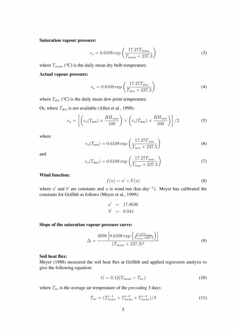
Saturation vapour pressure:
eo = 0.6108 exp
(17.27Tmean
Tmean + 237.3
)(3)
where Tmean (oC) is the daily mean dry bulb temperature.
Actual vapour pressure:
ea = 0.6108 exp
(17.27Tdew
Tdew + 237.3
)(4)
where Tdew (oC) is the daily mean dew point temperature.
Or, where Tdew is not available (Allen et al., 1998):
ea =
[(eo(Tmin)× RHmax
100
)+
(eo(Tmax)× RHmin
100
)]/2 (5)
where
eo(Tmin) = 0.6108 exp
(17.27Tmin
Tmin + 237.3
)(6)
and
eo(Tmax) = 0.6108 exp
(17.27Tmax
Tmax + 237.3
)(7)
Wind function:f(u) = a′ + b′(u) (8)
where a′ and b′ are constants and u is wind run (km day−1). Meyer has calibrated theconstants for Griffith as follows (Meyer et al., 1999):
a′ = 17.8636
b′ = 0.044
Slope of the saturation vapour pressure curve:
∆ =4098
[0.6108 exp
(17.27Tmean
Tmean+237.3
)]
(Tmean + 237.3)2(9)
Soil heat flux:Meyer (1988) measured the soil heat flux at Griffith and applied regression analysis togive the following equation:
G = 0.12(Tmean − Tav) (10)
where Tav is the average air temperature of the preceding 3 days:
Tav = (T i−1mean + T i−2
mean + T i−3mean)/3 (11)
5
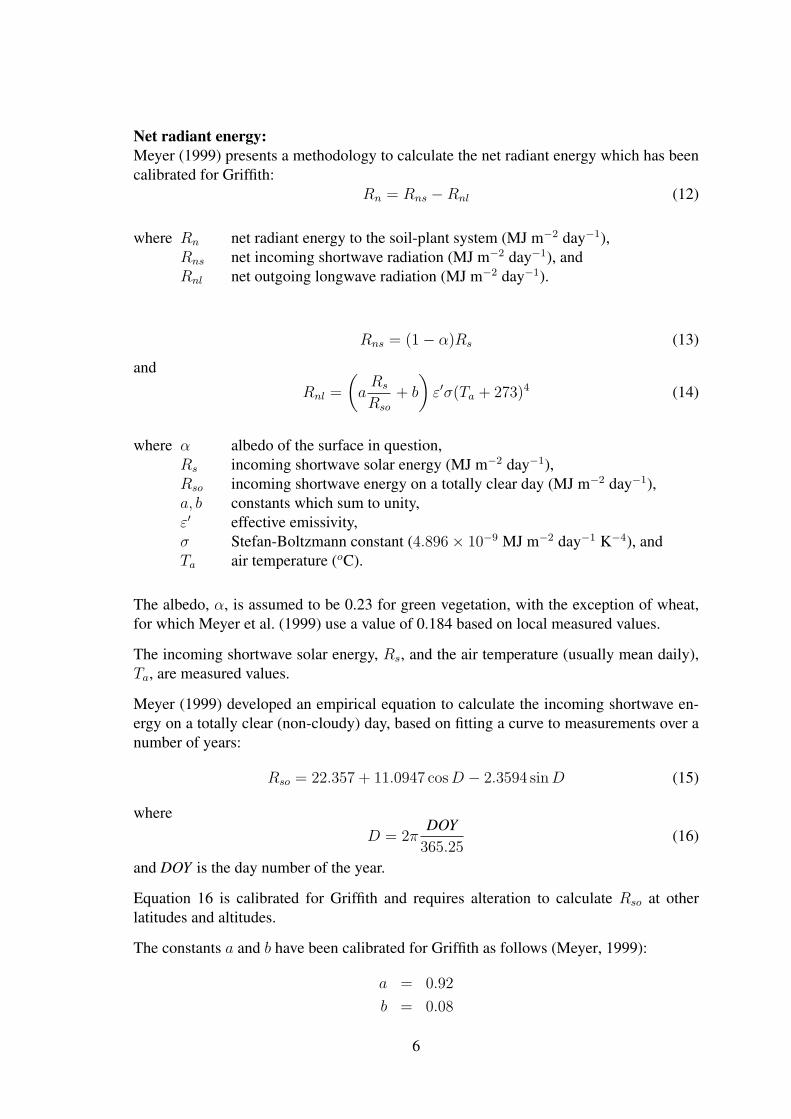
Net radiant energy:Meyer (1999) presents a methodology to calculate the net radiant energy which has beencalibrated for Griffith:
Rn = Rns −Rnl (12)
where Rn net radiant energy to the soil-plant system (MJ m−2 day−1),Rns net incoming shortwave radiation (MJ m−2 day−1), andRnl net outgoing longwave radiation (MJ m−2 day−1).
Rns = (1− α)Rs (13)
and
Rnl =
(a
Rs
Rso
+ b
)ε′σ(Ta + 273)4 (14)
where α albedo of the surface in question,Rs incoming shortwave solar energy (MJ m−2 day−1),Rso incoming shortwave energy on a totally clear day (MJ m−2 day−1),a, b constants which sum to unity,ε′ effective emissivity,σ Stefan-Boltzmann constant (4.896× 10⁻⁹ MJ m−2 day−1 K−4), andTa air temperature (oC).
The albedo, α, is assumed to be 0.23 for green vegetation, with the exception of wheat,for which Meyer et al. (1999) use a value of 0.184 based on local measured values.
The incoming shortwave solar energy, Rs, and the air temperature (usually mean daily),Ta, are measured values.
Meyer (1999) developed an empirical equation to calculate the incoming shortwave en-ergy on a totally clear (non-cloudy) day, based on fitting a curve to measurements over anumber of years:
Rso = 22.357 + 11.0947 cos D − 2.3594 sin D (15)
whereD = 2π
DOY365.25
(16)
and DOY is the day number of the year.
Equation 16 is calibrated for Griffith and requires alteration to calculate Rso at otherlatitudes and altitudes.
The constants a and b have been calibrated for Griffith as follows (Meyer, 1999):
a = 0.92
b = 0.08
6

The effective net emissivity, ε′ is given by:
ε′ = c + d√
ea (17)
where ea mean daily water vapour pressure in the air, andc, d constants with values 0.34 and -0.139 respectively.
3.2 The FAO Penman–Monteith method
3.2.1 The equation
The FAO Irrigation and Drainage Paper 56 Allen et al. (1998), produced by the Food andAgricultural Organisation of the United Nations, provides guidelines for estimating cropevapotranspiration based on the Penman–Monteith combination equation. This method istermed the “FAO Penman-Monteith”. Additional information can be sourced from Allenet al. (1998) and Dodds et al. (2005).
This method has been adopted by the Bureau of Meteorology for the calculation of ref-erence evapotranspiration values which are published as part of the SILO datasets. Thebasic equation is as follows:
Eto =0.408∆(Rn −G) + γ
(900
Tmean+273
)u2(eo − ea)
∆ + γ(1 + 0.34u2)(18)
where Eto daily reference evapotranspiration (mm day−1),∆ slope of saturation pressure curve (kPa oC−1),Rn net radiant energy to the soil-plant system (MJ m−2 day−1),G soil heat flux (MJ m−2 day−1),γ psychrometric constant (0.066 kPa oC−1),u2 daily mean wind speed at 2 m height (m s−1),eo mean daily saturation vapour pressure (kPa),ea actual mean daily vapour pressure (kPa), andTmean mean air temperature (oC).
3.2.2 Calculation of input variables
Formulæ and values for the input variables are given below. The formulæ and variablespresented here are those adopted for the calculation of Eto for the SILO evapotranspirationestimates (see Appendix A, Fitzmaurice and Beswick, 2005).
Saturation vapour pressure:The saturation vapour pressure at air temperature, T is:
e0(T ) = 0.6108 exp
(17.27T
T + 237.3
)(19)
7
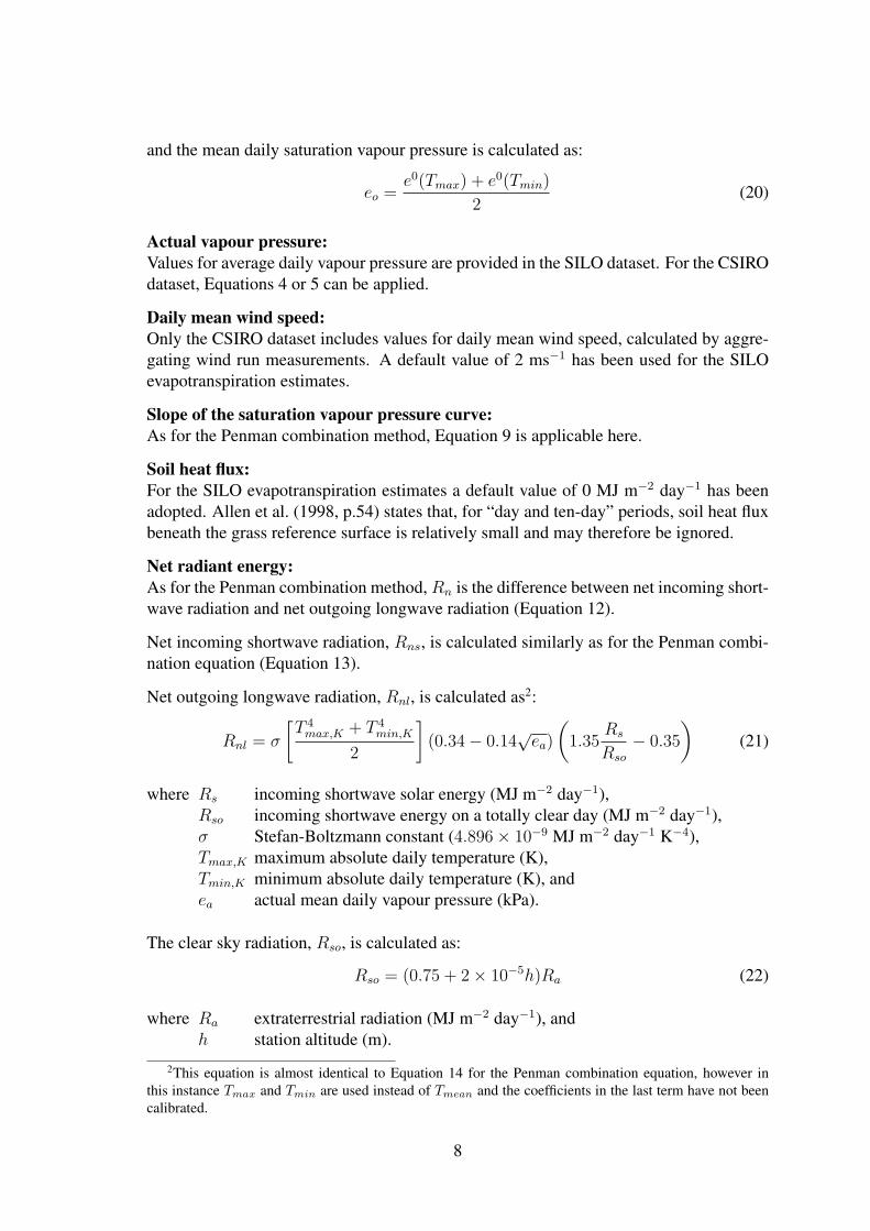
and the mean daily saturation vapour pressure is calculated as:
eo =e0(Tmax) + e0(Tmin)
2(20)
Actual vapour pressure:Values for average daily vapour pressure are provided in the SILO dataset. For the CSIROdataset, Equations 4 or 5 can be applied.
Daily mean wind speed:Only the CSIRO dataset includes values for daily mean wind speed, calculated by aggre-gating wind run measurements. A default value of 2 ms−1 has been used for the SILOevapotranspiration estimates.
Slope of the saturation vapour pressure curve:As for the Penman combination method, Equation 9 is applicable here.
Soil heat flux:For the SILO evapotranspiration estimates a default value of 0 MJ m−2 day−1 has beenadopted. Allen et al. (1998, p.54) states that, for “day and ten-day” periods, soil heat fluxbeneath the grass reference surface is relatively small and may therefore be ignored.
Net radiant energy:As for the Penman combination method, Rn is the difference between net incoming short-wave radiation and net outgoing longwave radiation (Equation 12).
Net incoming shortwave radiation, Rns, is calculated similarly as for the Penman combi-nation equation (Equation 13).
Net outgoing longwave radiation, Rnl, is calculated as2:
Rnl = σ
[T 4
max,K + T 4min,K
2
](0.34− 0.14
√ea)
(1.35
Rs
Rso
− 0.35
)(21)
where Rs incoming shortwave solar energy (MJ m−2 day−1),Rso incoming shortwave energy on a totally clear day (MJ m−2 day−1),σ Stefan-Boltzmann constant (4.896× 10⁻⁹ MJ m−2 day−1 K−4),Tmax,K maximum absolute daily temperature (K),Tmin,K minimum absolute daily temperature (K), andea actual mean daily vapour pressure (kPa).
The clear sky radiation, Rso, is calculated as:
Rso = (0.75 + 2× 10⁻⁵h)Ra (22)
where Ra extraterrestrial radiation (MJ m−2 day−1), andh station altitude (m).
2This equation is almost identical to Equation 14 for the Penman combination equation, however inthis instance Tmax and Tmin are used instead of Tmean and the coefficients in the last term have not beencalibrated.
8

The extraterrestrial radiation, Ra, is given by:
Ra =24× 60
πGscdr[ωs sin(ϕ) sin(δ) + cos(ϕ) cos(δ) sin(ωs)] (23)
where Gsc solar constant (0.0820 MJ m−2 min−1),dr inverse relative distance Earth–Sun,δ solar declination (rad),ϕ latitude (rad), andωs sunset hour angle (rad).
The terms in this equation can be calculated as follows:
dr = 1 + 0.033 cos
(J
2π
365
)(24)
where J is the number of the day in the year (between 1 and 365 or 366).
ωs = arccos(− tan(ϕ) tan(δ)) (25)
and
δ = 0.409 sin
(J
2π
365− 1.39
)(26)
9

4 Analysis Results
MS Excel spreadsheets and GenStat were used to manipulate the data and perform thecalculations. The results are presented here.
4.1 Results for the Penman–Griffith equation
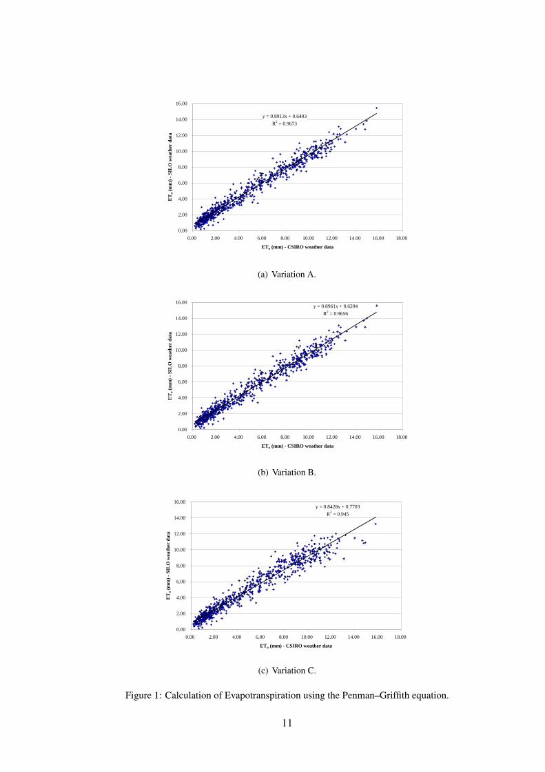
The CSIRO and SILO weather datasets were compared using the Penman–Griffith equa-tion. For the SILO weather dataset the following three variations were considered:
• Variation A: For the SILO dataset,(SILO0) soil heat flux (G) has been calculatedas for the Penman–Griffith equation and the CSIRO dataset wind speed values havebeen used in the wind function (f(u)).
• Variation B: For the SILO dataset (SILO1), soil heat flux (G) has been set to zeroand the CSIRO dataset wind speed values have been used in the wind function(f(u)).
• Variation C: For the SILO dataset (SILO2), soil heat flux (G) has been set to zeroand a default wind speed value of 2 ms−1 (or 172.8 km/day) has been used in thewind function (f(u)).
Reference evapotranspiration calculated using the SILO dataset were plotted against Etocalculated using the CSIRO dataset and the regression relationship obtained (refer Figure1). The results are summarised in Table 1. The regression value for which x = y [orEto(CSIRO) = Eto(SILO)] is also given.
Table 1: Summary of results for the Penman–Griffith equation.
Aunual Aggregate Eto (mm)Variation Regression Equationa R2 x = y 1989 1990
CSIRO SILO CSIRO SILOA y = 0.89x + 0.64 0.97 5.89 1834 1927B y = 0.90x + 0.62 0.97 5.97 1798 1836 1898 1929C y = 0.84x + 0.77 0.95 4.90 1764 1913
ay = Eto (SILO) and x = Eto (CSIRO)
The above results indicate only minor differences between Variations A and B. This is notsurprising when the values for G — as calculated using the CSIRO data and the Meyersoil heat flux equation — are examined. The average value for the assessment period is0.00, with a minimum value of -1.28 and a maximum value of 1.42. Hence approximatingG with a default value of zero, is not likely to introduce significant error.
10
y = 0.8913x + 0.6403
R2 = 0.9673
0.00
2.00
4.00
6.00
8.00
10.00
12.00
14.00
16.00
0.00 2.00 4.00 6.00 8.00 10.00 12.00 14.00 16.00 18.00
ETo (mm) - CSIRO weather data
ET
o (m
m)
- SI
LO
wea
ther
dat
a
(a) Variation A.
y = 0.8961x + 0.6204
R2 = 0.9656
0.00
2.00
4.00
6.00
8.00
10.00
12.00
14.00
16.00
0.00 2.00 4.00 6.00 8.00 10.00 12.00 14.00 16.00 18.00
ETo (mm) - CSIRO weather data
ET
o (m
m)
- SI
LO
wea
ther
dat
a
(b) Variation B.
y = 0.8428x + 0.7703
R2 = 0.945
0.00
2.00
4.00
6.00
8.00
10.00
12.00
14.00
16.00
0.00 2.00 4.00 6.00 8.00 10.00 12.00 14.00 16.00 18.00
ETo (mm) - CSIRO weather data
ET
o (m
m)
- SI
LO
wea
ther
dat
a
(c) Variation C.
Figure 1: Calculation of Evapotranspiration using the Penman–Griffith equation.
11

Annual Eto totals for all events analysed are given columns 5–8 of Table 1. InterestinglyVariations A and B show a consistent difference between the two datasets. Where wind isnot a factor of difference between the two datasets, the annual difference is approximately2%, with the SILO dataset overestimating Eto. When SILO wind is assumed to be adefault value of 2 ms−1, the differences become variable; for 1989 the difference was -2%and for 1990 the difference was almost 1%.
In Figure 2 the absolute difference between Eto calculated using the CSIRO datasetand Eto calculated using the SILO2 dataset (Var. C) has been plotted on a time scale.This plot shows that the difference between the two estimates is partially related to timewith Eto(SILO) on average being greater than Eto(CSIRO) during the winter months(March – September) and less than Eto(CSIRO) during the summer months (September– March). From this graph it can be appreciated that while on an annual basis the differ-ences between the two datasets is only small, on a seasonal basis the differences may befar more significant.
-3.00
-2.00
-1.00
0.00
1.00
2.00
3.00
4.00
5.00
14/09
/1988
23/12
/1988
2/04/1
989
11/07
/1989
19/10
/1989
27/01
/1990
7/05/1
990
15/08
/1990
23/11
/1990
3/03/1
991
Time
Abs
olut
e di
ffer
ence
(m
m):
Eto
-CSI
RO
- E
to-S
ILO
Figure 2: Absolute difference between Eto calculated using the CSIRO dataset and the SILO2dataset.
12
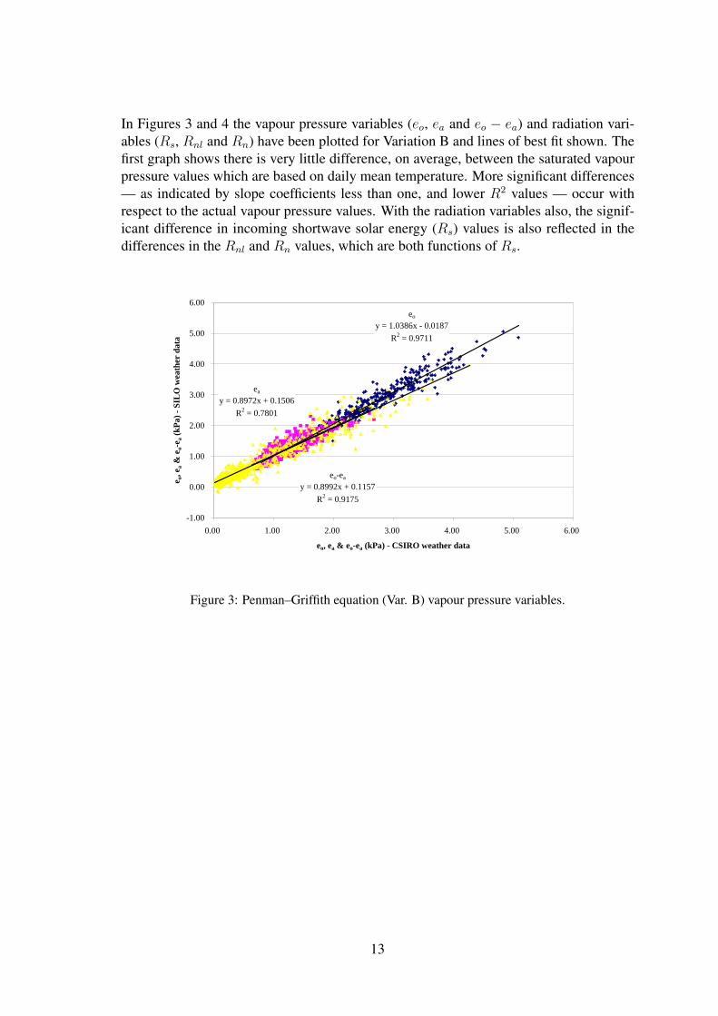
In Figures 3 and 4 the vapour pressure variables (eo, ea and eo − ea) and radiation vari-ables (Rs, Rnl and Rn) have been plotted for Variation B and lines of best fit shown. Thefirst graph shows there is very little difference, on average, between the saturated vapourpressure values which are based on daily mean temperature. More significant differences— as indicated by slope coefficients less than one, and lower R2 values — occur withrespect to the actual vapour pressure values. With the radiation variables also, the signif-icant difference in incoming shortwave solar energy (Rs) values is also reflected in thedifferences in the Rnl and Rn values, which are both functions of Rs.
eo
y = 1.0386x - 0.0187
R2 = 0.9711
ea
y = 0.8972x + 0.1506
R2 = 0.7801
eo-ea
y = 0.8992x + 0.1157
R2 = 0.9175
-1.00
0.00
1.00
2.00
3.00
4.00
5.00
6.00
0.00 1.00 2.00 3.00 4.00 5.00 6.00
eo, ea & eo-ea (kPa) - CSIRO weather data
e o, e
a &
eo-
e a (
kPa)
- S
ILO
wea
ther
dat
a
Figure 3: Penman–Griffith equation (Var. B) vapour pressure variables.
13

Rs
y = 0.8646x + 2.4907
R2 = 0.952
Rnl
y = 0.7215x + 1.5022
R2 = 0.8
Rn
y = 0.9292x + 0.6143
R2 = 0.9666
0.00
5.00
10.00
15.00
20.00
25.00
30.00
35.00
0.00 5.00 10.00 15.00 20.00 25.00 30.00 35.00 40.00
Rs, Rnl & Rn (MJ/m2/day) - CSIRO weather data
Rs
, Rnl
& R
n (M
J/m
2 /day
) -
SIL
O w
eath
er d
ata
Figure 4: Penman–Griffith equation (Var. B) radiation variables.
4.2 Results for the FAO Penman–Monteith equation
Results for the FAO Penman–Monteith equation are shown in Figure 5 and Table 2. Forthe SILO weather dataset the following variations were considered:
• Variation A: For the SILO dataset (SILO1), the CSIRO dataset wind speed valueshave been used.
• Variation B: For the SILO dataset (SILO2), a default wind speed value of 2 ms−1
(or 172.8 km/day) has been used.
As discussed in Section 3.2, a default value of zero has been adopted for soil heat flux, G— both for the CSIRO and SILO datasets.
Table 2: Summary of results for the FAO Penman–Monteith equation.
Annual Aggregate Eto (mm)Variation Regression Equationa R2 x = y 1989 1990
CSIRO SILO CSIRO SILOA y = 0.92x + 0.29 0.98 3.87 1383 1400
B y = 0.83x + 0.55 0.94 3.271380
13151400
1399
ay = Eto (SILO) and x = Eto (CSIRO)
14

y = 0.9255x + 0.2884
R2 = 0.9804
0.00
2.00
4.00
6.00
8.00
10.00
12.00
14.00
0.00 2.00 4.00 6.00 8.00 10.00 12.00 14.00 16.00
ETo (mm) - CSIRO weather data
ET
o (m
m)
- SI
LO
wea
ther
dat
a
(a) Variation A.
y = 0.8309x + 0.5531
R2 = 0.9363
0.00
2.00
4.00
6.00
8.00
10.00
12.00
14.00
0.00 2.00 4.00 6.00 8.00 10.00 12.00 14.00 16.00
ETo (mm) - CSIRO weather data
ET
o (m
m)
- SI
LO
wea
ther
dat
a
(b) Variation B.
Figure 5: Calculation of Evapotranspiration using the FAO Penman–Monteith equation.
Table 2 shows that for Variation A the annual ETo totals are almost identical for bothdatasets. Where wind is assumed to be a default value of 2 ms−1 (Var. B) the differencesbecome more variable (-5% for 1989 and 0% for 1990). This same phenomenon was alsoobserved in the case of the Penman–Griffith equation.
15
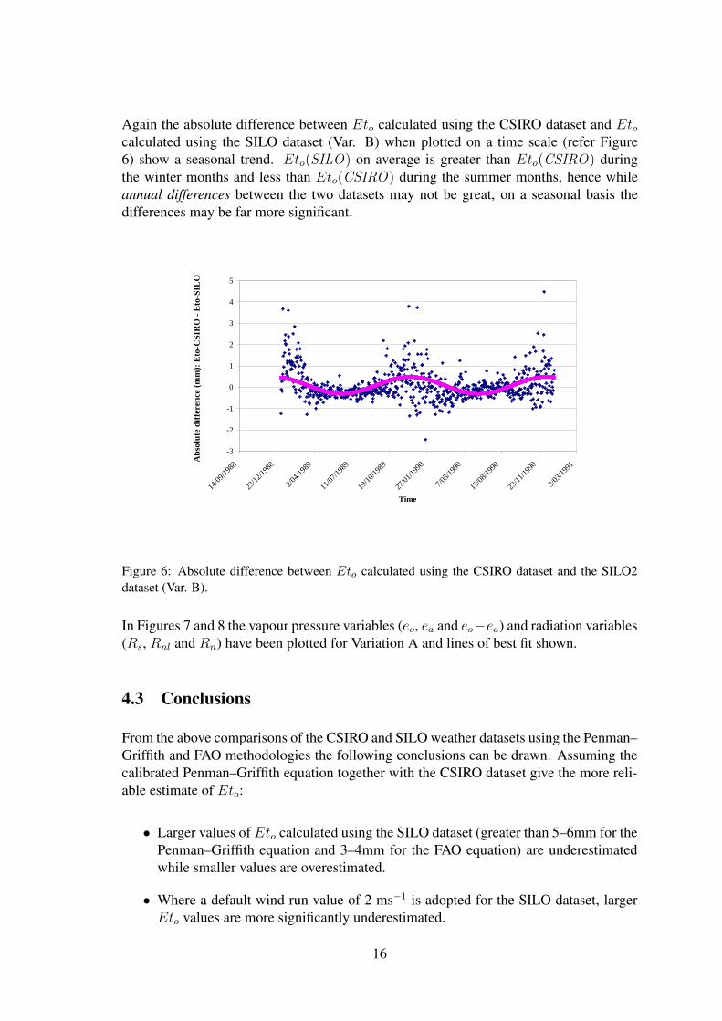
Again the absolute difference between Eto calculated using the CSIRO dataset and Etocalculated using the SILO dataset (Var. B) when plotted on a time scale (refer Figure6) show a seasonal trend. Eto(SILO) on average is greater than Eto(CSIRO) duringthe winter months and less than Eto(CSIRO) during the summer months, hence whileannual differences between the two datasets may not be great, on a seasonal basis thedifferences may be far more significant.
-3
-2
-1
0
1
2
3
4
5
14/09
/1988
23/12
/1988
2/04/1
989
11/07
/1989
19/10
/1989
27/01
/1990
7/05/1
990
15/08
/1990
23/11
/1990
3/03/1
991
Time
Abs
olut
e di
ffer
ence
(m
m):
Eto
-CSI
RO
- E
to-S
ILO
Figure 6: Absolute difference between Eto calculated using the CSIRO dataset and the SILO2dataset (Var. B).
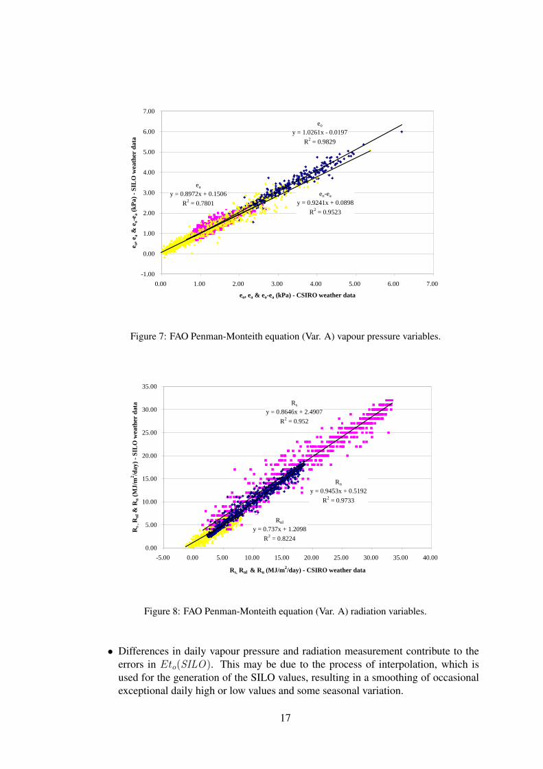
In Figures 7 and 8 the vapour pressure variables (eo, ea and eo−ea) and radiation variables(Rs, Rnl and Rn) have been plotted for Variation A and lines of best fit shown.
4.3 Conclusions
From the above comparisons of the CSIRO and SILO weather datasets using the Penman–Griffith and FAO methodologies the following conclusions can be drawn. Assuming thecalibrated Penman–Griffith equation together with the CSIRO dataset give the more reli-able estimate of Eto:
• Larger values of Eto calculated using the SILO dataset (greater than 5–6mm for thePenman–Griffith equation and 3–4mm for the FAO equation) are underestimatedwhile smaller values are overestimated.
• Where a default wind run value of 2 ms−1 is adopted for the SILO dataset, largerEto values are more significantly underestimated.
16
eo-ea
y = 0.9241x + 0.0898
R2 = 0.9523
ea
y = 0.8972x + 0.1506
R2 = 0.7801
eo
y = 1.0261x - 0.0197
R2 = 0.9829
-1.00
0.00
1.00
2.00
3.00
4.00
5.00
6.00
7.00
0.00 1.00 2.00 3.00 4.00 5.00 6.00 7.00
eo, ea & eo-ea (kPa) - CSIRO weather data
e o, e
a &
eo-
e a (
kPa)
- S
ILO
wea
ther
dat
a
Figure 7: FAO Penman-Monteith equation (Var. A) vapour pressure variables.
Rnl
y = 0.737x + 1.2098
R2 = 0.8224
Rn
y = 0.9453x + 0.5192
R2 = 0.9733
Rs
y = 0.8646x + 2.4907
R2 = 0.952
0.00
5.00
10.00
15.00
20.00
25.00
30.00
35.00
-5.00 0.00 5.00 10.00 15.00 20.00 25.00 30.00 35.00 40.00
Rs, Rnl & Rn (MJ/m2/day) - CSIRO weather data
Rs
, Rnl
& R
n (M
J/m
2 /day
) -
SIL
O w
eath
er d
ata
Figure 8: FAO Penman-Monteith equation (Var. A) radiation variables.
• Differences in daily vapour pressure and radiation measurement contribute to theerrors in Eto(SILO). This may be due to the process of interpolation, which isused for the generation of the SILO values, resulting in a smoothing of occasionalexceptional daily high or low values and some seasonal variation.
17

• Underestimation and overestimation of values is cyclic with underestimation oc-curring in the summer (high radiation; more advective) season and overestimationoccurring in the winter (low radiation; less advective) season.
• Where accurate wind values are adopted with the SILO dataset, the annual summa-tion of Eto is not affected by the less accurate dataset.
18

5 Comparison of Methods
In the preceding sections the differences in the Eto values calculated using two differentdatasets have been compared using two evapotranspiration methods. The first of thesemethods, the Penman–Griffith formula, has been locally calibrated using experimentaldata specific to Griffith; hence it can be considered to be the more precise method forthe Griffith locality. The second method, the FAO Penman–Monteith, is the standardrecommended by the Food and Agriculture Organisation of the United Nations which ispresently being used for calculation of the reference evapotranspiration values displayedon the SILO site.
Graphs comparing the two methods are presented in Figures 9 and 10. In both figuresEto calculated using the FAO method has been plotted against values calculated using thePenman–Griffith method. In Figure 9 the CSIRO dataset has been used for both methods.In Figure 10 the CSIRO dataset has been used with the Penman–Griffith method whilethe SILO2 datset (SILO values including a default wind speed of 2 ms−1) has been usedwith the FAO method.
y = 0.7091x + 0.2178
R2 = 0.9863
y = 0.7373x
R2 = 0.9839
0.00
2.00
4.00
6.00
8.00
10.00
12.00
14.00
0.00 2.00 4.00 6.00 8.00 10.00 12.00 14.00 16.00 18.00
Eto (mm): CSIRO weather data, Penman-Griffith method.
Et o
(m
m):
CSI
RO
wea
ther
dat
a, F
AO
met
hod.
Figure 9: A comparison between the Penman–Griffith and FAO Methods (CSIRO data only). Fullregression and regression through the origin shown.
19

y = 0.5965x + 0.6973
R2 = 0.9463
y = 0.6866x
R2 = 0.9133
0.00
2.00
4.00
6.00
8.00
10.00
12.00
14.00
0.00 2.00 4.00 6.00 8.00 10.00 12.00 14.00 16.00 18.00
Eto (mm): CSIRO weather data, Penman-Griffith Method.
Et o
(m
m):
SIL
O2
wea
ther
dat
a, F
AO
Met
hod.
Figure 10: A comparison between the Penman–Griffith (CSIRO data) and FAO (SILO2 data)Methods. Full regression and regression through the origin shown.
In order to confirm these results the procedure discussed in Section 4 was repeated usingCSIRO and SILO datasets for a second two year period: 2001–2002. The graphs for thisperiod, Figures 11 and 12, which correspond to those given in Figures 9 and 10, are givenbelow. These graphs verify the results obtained for the period 1989–1990.
y = 0.7114x + 0.1112
R2 = 0.9833
y = 0.7257x
R2 = 0.9827
0.00
2.00
4.00
6.00
8.00
10.00
12.00
14.00
0.00 2.00 4.00 6.00 8.00 10.00 12.00 14.00 16.00
Eto (mm): CSIRO weather data, Penman-Griffith method.
Et o
(m
m):
CSI
RO
wea
ther
dat
a, F
AO
met
hod.
Figure 11: A comparison between the Penman–Griffith and FAO Methods (CSIRO data only) forthe period 2001–2002. Full regression and regression through the origin shown.
20

y = 0.6083x + 0.5517
R2 = 0.9351
y = 0.6793x
R2 = 0.918
0.00
2.00
4.00
6.00
8.00
10.00
12.00
14.00
0.00 2.00 4.00 6.00 8.00 10.00 12.00 14.00 16.00
Eto (mm): CSIRO weather data, Penman-Griffith Method.
Et o
(m
m):
SIL
O2
wea
ther
dat
a, F
AO
Met
hod.
Figure 12: A comparison between the Penman–Griffith (CSIRO data) and FAO (SILO2 data)Methods for the period 2001–2002. Full regression and regression through the origin shown.
A summary of results is given in Table 3.
Table 3: Summary of results.
Regression Equationa Aggregate Eto (mm/yr)Equ. Data
1989-98 2001-02R2
1989 1990 2001 2002P–G CSIRO — — 1798 1898 2001 2228FAO CSIRO y = 0.71x + 0.22 y = 0.71x + 0.11 0.99 1385 1391 1473 1612FAO SILO1 y = 0.66x + 0.49 0.97 1383 1400 1493 1665FAO SILO2 y = 0.60x + 0.70 y = 0.61x + 0.55 0.95 1315 1399 1430 1546
ay = Eto (FAO) and x = Eto (P–G)
The results show that where the CSIRO dataset is used in the FAO Eto calculations, they-axis intercept for the line of best fit is relatively small. While statistically significant,the measure of improvement on the regression line placed though the origin is very small— less than 0.5%. Hence it can be generalised, that the FAO method consistently under-estimates Eto in comparison to the Penman–Griffith method by around 26%. Figure 13shows that this difference peaks at more than 2.5 mm per day in mid-summer. Use of theSILO dataset in the FAO Eto calculations results in an increase in the y-axis intercept anda decrease in slope. This means that daily Eto values calculated using the SILO weatherdata and FAO method will tend to be greater than the daily Eto values calculated usingCSIRO weather data and Penman–Griffith method at lower Eto and the opposite at highdaily Eto.
21
-1.00
-0.50
0.00
0.50
1.00
1.50
2.00
2.50
3.00
3.50
4.00
4.50
14/09
/1988
23/12
/1988
2/04/1
989
11/07
/1989
19/10
/1989
27/01
/1990
7/05/1
990
15/08
/1990
23/11
/1990
3/03/1
991
Time
Abs
olut
e di
ffer
ence
(m
m):
P-G
(CSI
RO
) -
FA
O(C
SIR
O)
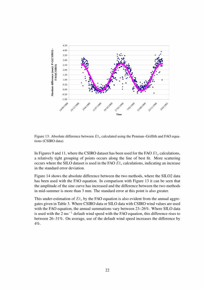
Figure 13: Absolute difference between Eto calculated using the Penman–Griffith and FAO equa-tions (CSIRO data).
In Figures 9 and 11, where the CSIRO dataset has been used for the FAO Eto calculations,a relatively tight grouping of points occurs along the line of best fit. More scatteringoccurs where the SILO dataset is used in the FAO Eto calculations, indicating an increasein the standard error deviation.
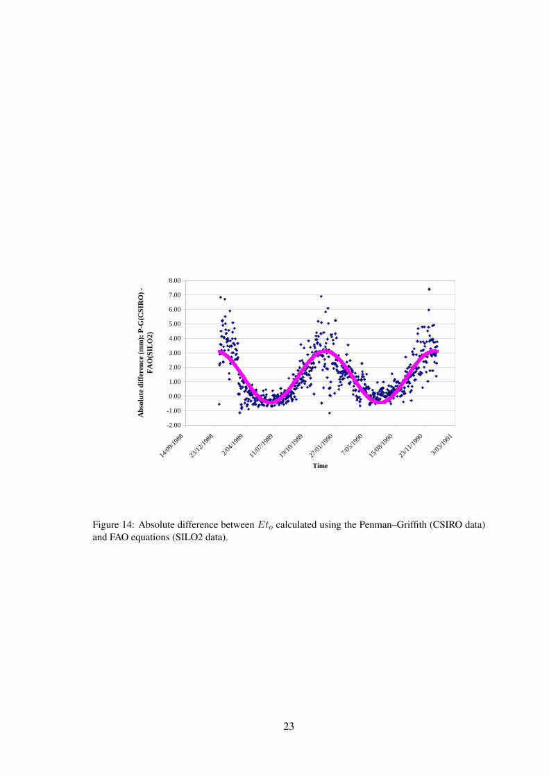
Figure 14 shows the absolute difference between the two methods, where the SILO2 datahas been used with the FAO equation. In comparison with Figure 13 it can be seen thatthe amplitude of the sine curve has increased and the difference between the two methodsin mid-summer is more than 3 mm. The standard error at this point is also greater.
This under-estimation of Eto by the FAO equation is also evident from the annual aggre-gates given in Table 3. Where CSIRO data or SILO data with CSIRO wind values are usedwith the FAO equation, the annual summations vary between 23–26%. Where SILO datais used with the 2 ms−1 default wind speed with the FAO equation, this difference rises tobetween 26–31%. On average, use of the default wind speed increases the difference by4%.
22
-2.00
-1.00
0.00
1.00
2.00
3.00
4.00
5.00
6.00
7.00
8.00
14/09
/1988
23/12
/1988
2/04/1
989
11/07
/1989
19/10
/1989
27/01
/1990
7/05/1
990
15/08
/1990
23/11
/1990
3/03/1
991
Time
Abs
olut
e di
ffer
ence
(m
m):
P-G
(CSI
RO
) -
FA
O(S
ILO
2)
Figure 14: Absolute difference between Eto calculated using the Penman–Griffith (CSIRO data)and FAO equations (SILO2 data).
23

6 Discussion and Conclusions
One of the aims of the National Evapotranspiration Project is the development of a stan-dardised method for the computation of reference evapotranspiration (Eto) using the lim-ited weather data typically available at weather stations across Australia. The analysesdescribed in this report have made an important contribution to this endeavour.
The SILO website provides limited meteorological datasets Australia-wide. These datasetsare currently being used with the FAO Penman–Monteith method to calculate local refer-ence evapotranspiration. Calculations use a default wind speed of 2 ms−1.
During the 1980s and 1990s, research was undertaken into evapotranspiration at theCSIRO station at Griffith, NSW. This work involved the collection of highly accurateweather data and led to the calibration of the Penman combination equation (Penman–Griffith) for the Griffith region.
This more precise methodology and dataset — the Penman–Griffith equation and CSIROweather data — have been compared with the FAO methodology and SILO dataset. Thiswork has shown that both the method and the dataset can contribute to differences in theresults.
When comparing the the two datasets, with either the Penman–Griffith or FAO equations,the absolute difference between the results is found to be cyclic with the CSIRO datasetgiving a higher value in summer (values greater than 5–6 mm) and the lower value inwinter (values less than 5–6 mm). When the annual aggregates are compared, differencesare not more than±2% — even where a default wind speed of 2 ms−1 is adopted with theSILO dataset — due to the cancelling effect of the seasonal differences. Hence it can beconcluded that any error in Eto estimation arising from the use of the SILO dataset willdepend on the period of interest. While annual estimates are not likely to be impacted,seasonal estimates may.
Results indicate, however, that the methodology is more critical than the dataset. Whenthe two methods are compared using the one, CSIRO, dataset, Eto values obtained usingthe FAO method are around 26% less than those obtained using the Penman–Griffithmethod. Use of the SILO dataset (including the default wind speed value) with the FAOequation, leads to increased differences particularly during the mid-summer period.
These differences are also reflected in the annual aggregates. Where CSIRO data or SILOdata with CSIRO wind values are used with the FAO equation, the annual summationsvary between 23–28%. Where SILO data is used with the 2 ms−1 default wind speedwith the FAO equation, this difference rises by approximately 3%. This increase wouldbe greater during the summer season and less during the winter season.
It is acknowledged that the results presented here relate to a single Australian locality —Griffith, NSW. In order to ascertain whether these result are applicable for Australia ingeneral, further research is required. Investigations and results relating to other localitieswill follow in the Part 2 of this report.
24
ReferencesAllen, R. G., Pereira, L. S., Raes, D., and Smith, M. (1998). Crop evapotranspiration.
Guidelines for computing crop water requirements. FAO Irrigation and Drainage Pa-per 56, Food and Agriculture Organization of the United Nations, Rome.
Bureau of Meteorology (2005). Patched point dataset. Internet: www.bom.gov.au/si-lo/ProductIndex.shtml, viewed 6 June.
Dodds, P., Meyer, W., and Barton, A. (2005). A review of methods to estimate irrigatedreference crop evapotranspiration across Australia. Technical Report 04/05, CRC forIrrigation Futures and CSIRO Land and Water, Adelaide, SA.
Fitzmaurice, L. and Beswick, A. (2005). Sensitivity of the FAO56 crop reference evap-otranspiration to different input data. Technical Report LWA QNR-37, Department ofNatural Resources and Mines, Queensland.
Jeffrey, S. J., Carter, J. O., Moodie, K. M., and Beswick, A. R. (2001). Using spatialinterpolation to construct a comprehensive archive of Australian climate data. In Envi-ronmental Modelling and Software, volume 16, pages 309–330. Elsevier.
Meyer, W. S. (1988). Development of management strategies for minimizing salinizationdue to irrigation: Quantifying components of the water balance under irrigated crops.AWRAC Research Project 84/162, CSIRO, Griffith, NSW.
Meyer, W. S. (1999). Standard reference evaporation calculation for inland, south easternAustralia. Technical Report 35/98, CSIRO Land & Water, Adelaide, SA.
Meyer, W. S., Smith, D. J., and Shell, G. (1999). Estimating reference evaporation andcrop evapotranspiration from weather data and crop coefficients. Technical Report34/98, CSIRO Land & Water, Adelaide, SA. An addendum to AWRAC ResearchProject 84/162.
Penman, H. L. (1948). Natural evaporation from open water, bare soil and grass. InProceedings of the Royal Society of London, volume 193 of A, pages 120–146.
Shell, G. S., Meyer, W. S., and Smith, D. J. (1997). Guidelines on installation and main-tenance of low cost automatic weather stations with particular reference to the mea-surement of wet bulb temperature in arid climates and the calculation of dew pointtemperature. Technical Report 28/97, CSIRO Land and Water, Griffith.
25

PO Box 56, Darling Heights Qld 4350 | Phone: 07 4631 2046 | Fax: 07 4631 1870 | Web: www.irrigationfutures.org.au
Partner Organisations