an analysis of stresses and displacements around a fault

Southern Illinois University CarbondaleOpenSIUC

Theses Theses and Dissertations

5-1-2018

An Analysis of Stresses and Displacements arounda Fault Plane Due to Longwall Face Advance inCoal MiningCorbin Grant CarltonSouthern Illinois University Carbondale, [email protected]

Follow this and additional works at: https://opensiuc.lib.siu.edu/theses

This Open Access Thesis is brought to you for free and open access by the Theses and Dissertations at OpenSIUC. It has been accepted for inclusion inTheses by an authorized administrator of OpenSIUC. For more information, please contact [email protected].

Recommended CitationCarlton, Corbin Grant, "An Analysis of Stresses and Displacements around a Fault Plane Due to Longwall Face Advance in CoalMining" (2018). Theses. 2325.https://opensiuc.lib.siu.edu/theses/2325

https://opensiuc.lib.siu.edu?utm_source=opensiuc.lib.siu.edu%2Ftheses%2F2325&utm_medium=PDF&utm_campaign=PDFCoverPages

https://opensiuc.lib.siu.edu/theses?utm_source=opensiuc.lib.siu.edu%2Ftheses%2F2325&utm_medium=PDF&utm_campaign=PDFCoverPages

https://opensiuc.lib.siu.edu/etd?utm_source=opensiuc.lib.siu.edu%2Ftheses%2F2325&utm_medium=PDF&utm_campaign=PDFCoverPages

https://opensiuc.lib.siu.edu/theses?utm_source=opensiuc.lib.siu.edu%2Ftheses%2F2325&utm_medium=PDF&utm_campaign=PDFCoverPages

https://opensiuc.lib.siu.edu/theses/2325?utm_source=opensiuc.lib.siu.edu%2Ftheses%2F2325&utm_medium=PDF&utm_campaign=PDFCoverPages

mailto:[email protected]

AN ANALYSIS OF STRESSES AND DISPLACEMENTS AROUND A FAULT PLANE DUE

TO LONGWALL FACE ADVANCE IN COAL MINING

By

Corbin Carlton

B.S., Southern Illinois University Carbondale, 2012

A Thesis Submitted in Partial

Fulfillment of the Requirements

for the Degree of

Master in Science

in the field of Mining Engineering

Department of Mining and Mineral Resource Engineering

Southern Illinois University Carbondale

May 2018

THESIS APPROVAL



By

Corbin Carlton

A Thesis Submitted in Partial

Fulfillment of the Requirements

for the Degree of

Master in Science

in the field of Mining Engineering

Approved by:

Dr. Yoginder P. Chugh, Thesis Chair, MMRE

Dr. Joseph C. Hirschi MMRE

Dr. Tsuchin P. Chu, MEEP

Dr. Prabir K. Kolay, CE

Graduate School

Southern Illinois University Carbondale

May 2018

i

AN ABSTRACT OF THE THESIS OF

Corbin Carlton, for the Master of Science degree in Mining Engineering, presented on April 2nd

2018, at Southern Illinois University Carbondale.



MAJOR PROFESSOR: Dr. Yoginder P. Chugh

This study has examined 3D stresses and displacements around a longwall mining system

that is intercepted by a geological fault. More specifically, the study has analyzed the effect of a

fault on longwall gate development entries, set-up rooms, T-junctions, and the longwall face as

the longwall face progressed toward, through, and away from the fault. A general lithologic

sequence and mining parameters related to the Herrin No. 6 coal seam in southern Illinois were

employed. FLAC3D structural analysis code was used for simulating two (2) adjacent longwall

faces. Linear elastic rock mass elements with non-linear elastic-plastic fault elements were

analyzed using Hoek- Brown brittle failure criteria. Two (2) models were developed for

analysis: a base elastic case without fault and an elastic model with elastic-plastic fault elements.

Engineering properties for the rock mass strata were derived from a history of rock core testing

and modified following the process indicated for Hoek’s Geologic Strength Index. Gob

engineering properties and estimated load carrying capacities developed in earlier studies were

used to make simulations physically realistic. The local tectonic (horizontal) stress field and

vertical stress levels were applied to the simulation boundaries.

Analysis data was extracted for several data lines in the roof and floor that were

determined to be critical based on the geometry of the mine layout. Extracted data included 3D

stresses and displacements with the Z-direction indicating vertical. This data was used to

calculate vertical convergence and vertical and horizontal stress concentration variables VSCF,

ii

HSCF-XX, and HSCF-YY. Such data were developed for the longwall face advancing in 30-foot

(10-m) increments away from the set-up room.

Incremental displacements due to the fault proved to be more significant than changes in

stress concentrations VSCF, HSCF-XX, and HSCF-YY. Set-up room X-displacements show a

consistent increase in the fault case around 35%. Incremental Y-displacements vary sharply at

first then changes quickly reduce to zero (0). Z-displacements were similar in both models. A

fault oriented more vertically would have larger Z-displacement values.

Gate X-displacements significantly decrease in the fault model until the face reaches 558

feet (170 m) from the starting point. Y-displacements show a rapid percentage rise in the fault

model as the longwall face approaches the intersection of the fault with the first gate entry, but

significant percentage decreases both before and after reaching this intersection. Significant

increases in Z-displacements occur as the face approaches and leaves the intersection of the fault

with the gate entries.

Around the fault, the first row of gate pillars experiences a change in horizontal

displacements HSCF-XX and HSCF-YY of approximately 10%. Second row pillars also see a

change in HSCF-XX of around 10%, but not a significant change in HSCF-YY. Gate entry

VSCF values show significant increases at the fault intersection until the face passes the

gate/fault intersection.

iii

DEDICATION

To my family

iv

ACKNOWLEDGEMENTS

I would like to thank Dr. Joseph C. Hirschi for the time that he took to review my work. His

review not only included grammar and checks for consistency, but also was educational in regard to

lessons in technical writing. Thank you Dr. Hirschi for both the quality of the review and the time you

have dedicated to it.

Thank you, Harrold Gurley and Richard Lyon, for gathering the field data and our visits together

to the mines. The trips were educational, impactful, and in one instance quite frightening. I will never

forget being far from the ramp in a coal and having to make it back by turning off the vehicles headlights

to conserve power in the battery. Going with you both down to the longwall mining areas gave me the

ground level perspective of what the models in this work represent.

It is important that I thank my wife, Shaylin Carlton, for helping to maintain order in my life as I

pressed onward to complete my master’s while working full-time.

I started this journey 6 years ago. As an undergraduate I made the decision to sign up for an M.S.

under Dr. Chugh. He and I have spent many hours together throughout this project. I’ve had the

privilege to be his TA for 3 MNGE-431 courses, and the opportunity to work with Dr. Chugh on articles.

His encouragement is reason why I was able to complete this document. No matter how much or how

often I allowed life to get in the way, his persistence and willingness to get me through the M.S. program

kept me focused and kept me going. Thank you Dr. Chugh for choosing me as a student, giving me the

opportunities to teach students, spending hours going over concepts and analysis, and for not giving up on

me.

v

TABLE OF CONTENTS

CHAPTER PAGE

ABSTRACT ..................................................................................................................................... i

DEDICATION ............................................................................................................................... iii

ACKNOWLEDGEMENTS ........................................................................................................... iv

TABLE OF CONTENTS .................................................................................................................v

LIST OF TABLES ......................................................................................................................... ix

LIST OF FIGURES ...................................................................................................................... xii

CHAPTER 1: INTRODUCTION ....................................................................................................1

1.1 Background ................................................................................................................................1

1.2 Problem Statement .....................................................................................................................3

1.3 Goals and Specific Objectives ...................................................................................................5

1.4 Significance of the Study ...........................................................................................................6

1.5 Thesis Structure .........................................................................................................................7

CHAPTER 2: LITERATURE REVIEW .........................................................................................9

2.1 Overview of the Longwall Mining Method ...............................................................................9

2.2 Ground Control Around Longwall Mining Areas ...................................................................11

2.2.1 Gate Entries ..........................................................................................................................12

2.2.2 Face Area ..............................................................................................................................14

vi

2.2.3 Gob Area ...............................................................................................................................15

2.3 Numerical Modeling of Longwall Mining Areas ....................................................................16

2.3.1 Development of Rock Mass Properties for Modeling ...........................................................18

2.3.2 Intact Rock and Rock Mass Mechanical Behavior ...............................................................19

2.3.3 Hoek-Brown Failure Criterion .............................................................................................23

2.3.4 Mohr-Coulomb Failure Criterion for Intact Rock ................................................................26

2.4 Stress Redistribution and Mechanisms of Failure ...................................................................27

2.5 Numerical Modeling of Geologic Anomalies and Faults in Longwall Mining .......................28

2.5.1 Difficulties Associated with Modeling Geologic Anomalies Numerically ............................29

2.6 Fault Modeling Using UJRM Technique .................................................................................30

2.7 Modeling of Caved Gob in Longwall Mining .........................................................................31

2.8 Experimental Approaches for Assessment of Caving .............................................................31

2.8.1 Analytical Approach .............................................................................................................31

2.8.2 Empirical Approach ..............................................................................................................32

2.8.3 Numerical Approach .............................................................................................................32

CHAPTER 3: MODEL DEVELOPMENT AND FIELD MONITORING STUDIES .................34

3.1 Description of Physical Problem and Mine Environment .......................................................34

3.2 Identification of Areas to be Modeled .....................................................................................36

vii

3.2.1 Development of Numerical Models .......................................................................................38

3.2.2 Immediate Roof and Floor Lithology of Models ...................................................................39

3.3 Model and Engineering Properties Development ....................................................................40

3.3.1 Model Size .............................................................................................................................41

3.3.2 Engineering Properties of Intact Rocks ................................................................................41

3.3.3 Additional Engineering Properties .......................................................................................42

3.3.4 Development of Strata Properties Along the Fault...............................................................44

3.3.5 Modeling of Face Advance ...................................................................................................44

3.3.6 Simulation of Gob Loading Characteristics and Longwall Hydraulic Supports ..................45

3.3.7 Stress Concentration Factors ...............................................................................................47

3.3.8 Model Validation ..................................................................................................................47

3.3.9 Minimizing Modeling Errors ................................................................................................50

3.4 In-Mine Geotechnical Studies ..................................................................................................50

3.5 Limitations of Model Development and Analysis ...................................................................53

3.6 Analysis of Data from Numerical Modeling ...........................................................................54

3.6.1 Displacement Variables ........................................................................................................54

CHAPTER 4: ANALYTICAL STUDIES .....................................................................................56

4.1 Model Analysis ........................................................................................................................56

viii

4.2 Analysis of Set-up Room Entries Intersected by the Fault ......................................................57

4.2.1 Model Comparisons at 100 feet (30 m) of Face Advance .....................................................57

4.2.2 Results Summary of Set-up Room Analysis ...........................................................................63

4.3 Analysis of Gate Entries Intersected by the Fault ....................................................................70

4.3.1 Model Comparisons at 558 feet (170 m) of Face Advance ...................................................70

4.3.2 Results Summary of Face Advance Analysis ......................................................................105

4.3.3 Results Summary of Gate Entry Analysis ............................................................................106

4.4 Comparison of Model 2 and Field Results for Gate Entries Intersected by Fault .................109

CHAPTER 5: CONCLUSIONS AND RECOMMENDATIONS ..............................................111

5.1 Summary of Research ............................................................................................................111

5.2 Summary of Results ...............................................................................................................112

5.2.1 Displacements in Areas where Fault Intersects Set-up Rooms ..........................................112

5.2.2 Displacements in Areas where Fault Intersects Gate Development Entries ......................113

5.3 Recommendations for Additional Research ..........................................................................114

BIBLIOGRAPHY ........................................................................................................................115

VITA ............................................................................................................................................123

ix

LIST OF TABLES

TABLE PAGE

2.1 Common GSI ranges for typical rock formations (Marinos and Hoek, 2000) ..................25

3.1 Engineering properties of rock strata used in modeling. ...................................................40

4.1 Average results for B-B’ data line within ±9.83 feet (3 m) of intersection with fault for 0

to 200 feet (60 m) of face advance.....................................................................................64

4.2 Average results for C-C’ data line within ±9.83 feet (3 m) of intersection with fault for 0


4.3 Average results for A-A’ data line within ±9.83 feet (3 m) of intersection with face for 0


4.4 Average results for J-J’ data line within ±9.83 feet (3 m) of intersection with fault for 0


4.5 Average results for A-A’ data line within ±9.83 feet (3 m) of intersection with the lateral

face location for Model 1 advancing from 230 feet (70 m) through 1050 feet (320 m) ....84

4.6 Average results for A-A’ data line within ±9.83 feet (3 m) of intersection with the lateral

face location for Model 2 advancing from 230 feet (70 m) through 1050 feet (320 m) ....85

4.7 Percent change between Models 1 and 2 for A-A’ data line within ±9.83 feet (3 m) of

Model 2 fault intersection for face advancing from 230 feet (70 m) through 1050 feet

(320 m) ...............................................................................................................................86

4.8 Average results for Model 1 J-J’ data line within ±9.83 feet (3 m) of intersection with

Model 2 fault for face advancing from 230 feet (70 m) through 1050 feet (320 m) .........87

x

4.9 Average results for Model 2 J-J’ data line within ±9.83 feet (3 m) of intersection with


4.10 Percent change in J-J’ data line within ±9.83 feet (3 m) of Model 2 fault intersection for

face advancing from 230 feet (70 m) through 1050 feet (320 m) ......................................89

4.11 Average results for Model 1 E-E’ data line within ±9.83 feet (3 m) of intersection with


4.12 Average results for Model 2 E-E’ data line within ±9.83 feet (3 m) of intersection with


4.13 Percent change on E-E’ within ±9.83 feet (3 m) of intersection with Model 2 fault for


4.14 Average results for Model 1 F-F’ data line within ±9.83 feet (3 m) of intersection with


4.15 Average results for Model 2 F-F’ data line within ±9.83 feet (3 m) of intersection with


4.16 Percent change on F-F’ within ±9.83 feet (3 m) of intersection with Model 2 fault for face

advancing from 230 feet (70 m) through 1050 feet (320 m) .............................................95

4.17 Average results for Model 1 G-G’ data line within ±9.83 feet (3 m) of intersection with


4.18 Average results for Model 2 G-G’ data line within ±9.83 feet (3 m) of intersection with


4.19 Percent change on G-G’ within ±9.83 feet (3 m) of intersection with Model 2 fault for


xi

4.20 Average results for Model 1 H-H’ data line within ±9.83 feet (3 m) of intersection with


4.21 Average results for Model 2 H-H’ data line within ±9.83 feet (3 m) of intersection with

Model 2 fault for face advancing from 230 feet (70 m) through 1050 feet (320 m) .......100

4.22 Percent change on H-H’ within ±9.83 feet (3 m) of intersection with Model 2 fault for

face advancing from 230 feet (70 m) through 1050 feet (320 m) ....................................101

4.23 Average results for Model 1 I-I’ data line within ±9.83 feet (3 m) of intersection with


4.24 Average results for Model 2 I-I’ data line within ±9.83 feet (3 m) of intersection with


4.25 Percent change on I-I’ within ±9.83 feet (3 m) of intersection with Model 2 fault for face

advancing from 230 feet (70 m) through 1050 feet (320 m) ...........................................104

xii

LIST OF FIGURES

FIGURE PAGE

1.1 Example layout of adjacent longwall panels .......................................................................2

1.2 Rock mass supported by longwall shield support (Whittaker and Reddish, 1989) .............3

1.3 Faults in southern Illinois (from Nelson 1981) ....................................................................4

1.4 Average annual production per longwall mine and the number of longwall mines in the

US, 1992 – 2013 (Weir United States Longwall Mining Statistics) ....................................6

2.1 Depiction of both mining methods being used at a longwall mining operation ................10

2.2 Distribution of loading about the longwall panel (Peng and Chiang, 1984) .....................13

2.3 Caving and displacement of roof strata due to longwall face advance (Kolebaevna, 1968)

............................................................................................................................................15

2.4 Five (5) zones associated with caving, proposed by Duplancic and Brady (1999) ...........16

2.5 Example of an intact rock sample ......................................................................................20

2.6 Example of a stress-strain curve for an intact rock sample ...............................................20

2.7 Stress-strain curve for a brittle material ............................................................................21

2.8 Stress strain curve for strain-hardening (upper) and strain-softening (lower) material .....21

2.9(a) Mohr’s circles from tri-axial testing ..................................................................................22

2.9(b) Generalized non-linear failure envelope. ...........................................................................22

2.9(c) Idealized linear failure envelope if a = 1 (Navier-Coulomb). ............................................22

2.10 Hoek-Brown failure envelope for rock mass strength (σ1 and σ3 planes) .........................24

xiii

2.11 Envelope in Mohr-space using σ1 and σ3 planes ................................................................26

2.12 Stress redirection about the roadway caused by localized rock failure and subsequent

changes in bulk material properties during roadway development (Gale, 2005) ..............29

3.1 Fault and ground movement monitoring station locations in (a) Headgate of case study

panel, and (b) Headgate of adjoining longwall panel for first fault zone ..........................35

3.2 (a) Cross-sectional view of second fault/graben area in headgate return entry of case study

panel, and (b) Plan view of same area showing ground movement monitoring locations 36

3.3 Layout and dimensions of the modeled mining environment. ...........................................37

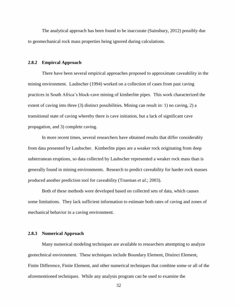
3.4 Area modeled at coal seam level with fault zone highlighted ..........................................38

3.5 Side view of longwall hydraulic support ..........................................................................45

3.6 Gob loading characteristics simulated in numerical models .............................................46

3.7 Set-up room geometry showing fault location and model validation cross-sections.........48

3.8 Validation comparison left of fault displacement in z-direction ......................................49

3.9 Comparison of VSC along the fault line (A-A’) ................................................................49

3.10 Residual error as a function of number of iterations ..........................................................50

3.11 Southeastern Illinois mine panel where field observations were made .............................51

3.12 Example of crib rosette used for measuring rock mass distortion .....................................52

3.13 Example of roof-to-floor converge results as mining advances ........................................52

3.14 Location of faults and measurement points ......................................................................53

3.15 Modeled area with primary data lines used for analysis ...................................................55

xiv

4.1 Model depiction with principal data lines (purple), fault zone (green), and face advance

distances (red and yellow) .................................................................................................56

4.2 Data lines (purple) and fault (green) at 100 feet (30 m) of face advance (gray) ...............57

4.3 VSCF-ZZ in Models 1 and 2 along B-B’ after 100 feet (30 m) of face advance ..............58

4.4 X-displacements in Models 1 and 2 at B-B’/A-A’ intersection for advancing face ..........58

4.5 Y-displacements in Models 1 and 2 at B-B’/A-A’ intersection for advancing face ..........59

4.6 X-displacements in Models 1 and 2 at C-C’/A-A’ intersection for advancing face ..........59

4.7 Y-displacements in Models 1 and 2 at C-C’/A-A’ intersection for advancing face ..........60

4.8 Y-displacements in Models 1 and 2 at C-C’/A-A’ intersection after 100 feet (30 m) of

face advance .......................................................................................................................60

4.9 X-displacements in Models 1 and 2 at A-A’/J-J’ intersection for advancing face ............61

4.10 Y-displacements in Models 1 and 2 at A-A’/J-J’ intersection for advancing face ............61

4.11: VSCF-ZZ in Model 2 along A-A’ after 100 feet (30 m) of face advance .........................62

4.12: X-displacements in Models 1 and 2 along J-J’ after 100 feet (30 m) of face advance ......62

4.13: X-displacements in Models 1 and 2 at J-J’/A-A’ intersection for advancing face ............63

4.14: Y-displacements in Models 1 and 2 at J-J’/A-A’ intersection for advancing face ............63

4.15: X-displacements in Models 1 and 2 at the fault/face intersection for face advancing from

230 feet (70 m) through 1050 feet (320 m) ........................................................................71

4.16: Y-displacements in Models 1 and 2 at the fault/face intersection for face advancing from


xv

4.17: Z-displacements in Models 1 and 2 at the fault/face intersection for face advancing from


4.18: HSCF-XX for A-A’ after 558 feet (170 m) of face advance ............................................72

4.19: X-displacements in Models 1 and 2 at the face/fault intersection for face advancing from


4.20: Y-displacements in Models 1 and 2 at the face/fault intersection for face advancing from


4.21: Z-displacements in Models 1 and 2 at the face/fault intersection for face advancing from


4.22: HSCF-XX for J-J’ after 558 feet (170 m) of face advance ...............................................74

4.23: Model 2 vectors showing horizontal displacement around face/fault intersection for 558

feet (170 m) of face advance ..............................................................................................75

4.24: Model 2 vectors showing horizontal displacement around gate-entry intersection with

fault for 558 feet (170 m) of face advance .........................................................................75

4.25: X-displacements in Models 1 and 2 at the face/fault intersection of E-E’ for face


4.26: Y-displacements in Models 1 and 2 at the face/fault intersection of E-E’ for face


4.27: Z-displacements in Models 1 and 2 at the face/fault intersection of E-E’ for face


4.28: Z-displacement of E-E’ after 558 feet (170 m) of face advance .......................................77

xvi

4.29: X-displacements in Models 1 and 2 at the face/fault intersection of F-F’ for face


4.30: Y-displacements in Models 1 and 2 at the face/fault intersection of F-F’ for face


4.31: Z-displacements in Models 1 and 2 at the face/fault intersection of F-F’ for face


4.32: X-displacements in Models 1 and 2 at the face/fault intersection of G-G’ for face


4.33: Y-displacements in Models 1 and 2 at the face/fault intersection of G-G’ for face


4.34: Z-displacements in Models 1 and 2 at the face/fault intersection of G-G’ for face


4.35: VSCF-ZZ of G-G’ after 558 feet (170 m) of face advance ..............................................80

4.36: X-displacements in Models 1 and 2 at the face/fault intersection of H-H’ for face


4.37: Y-displacements between Models 1 and 2 at the face/fault intersection of H-H’ for face


4.38: Z-displacements in Models 1 and 2 at the face/fault intersection of H-H’ for face


4.39: X-displacements in Models 1 and 2 at the face/fault intersection of I-I’ for face advancing

from 230 feet (70 m) through 1050 feet (320 m) ...............................................................82

xvii

4.40: Y-displacements in Models 1 and 2 at the face/fault intersection of I-I’ for face advancing


4.41: Z-displacements in Models 1 and 2 at the face/fault intersection of I-I’ for face advancing


4.42: Mine map of gate entries showing fault intersection and observation points .................109

4.43: Points 11 and 13 results for model and physical mining environment ...........................110

1

CHAPTER 1

INTRODUCTION

1.1. Background

Historically, coal reserves that are closer to the surface are more economical to mine than

coal that is deeper underground. Within the Illinois coal basin, near-surface economically

mineable coal has largely been extracted. Currently, most of the coal mined in the Illinois coal

basin comes from underground coal mines. The need for coal as an energy source remains

strong in today’s society; however, mining deeper coal reserves under adverse conditions

presents challenges, particularly in regions where geological anomalies such as faults, folds, and

dipping seams are present.

Due to economic and productivity pressures, several Illinois coal mines have determined

that the longwall mining method (Figure 1.1) is worth the risk of the large capital investment

required to pursue it. To mine coal using this method, development entries are driven from main

entries along both sides of a block of coal and connected at the end by “set-up rooms” to

establish the longwall face, which can be 900 to 1500 feet (274-457 m) long depending upon

mining conditions and desired output. A slice of coal approximately 3-foot (1 m) wide is

extracted each time the longwall shearer or plow travels the length of the face. Loosened coal

falls off the face onto an armored face conveyor (AFC) chain. It travels in the AFC along the

length of the face and is dumped onto a main belt conveyor through a stage loader and crusher.

The belt conveyor carries run-of-mine coal to the surface where it may be processed and

stockpiled prior to being shipped to the customer.

2

Figure 1.1: Example layout of adjacent longwall panels.

Along the entire length of the longwall face, the roof is supported by hydraulic steel

supports called shields. These supports are advanced incrementally as coal is extracted. As

supports advance, strata above the coal seam is allowed to cave and form a fractured gob

material behind the face shields (Figure 1.2).

Longwall face advance rates have increased over time and are currently averaging 90 feet

(27 m) per day with peak rates of 100 to 110 feet per day (30-35 m). This results in highly

dynamic stress and displacement environments along the face and in the caving area behind the

face. Mining companies must plan for ground control in the face area and in development areas

to minimize production losses and maximize the safety of mine workers and equipment.

3

Figure 1.2: Rock mass supported by longwall shield support (Whittaker and Reddish, 1989).

1.2 Problem Statement

The longwall mining method is a very productive mining system capable of producing in

excess of 20,000 clean tons per day. It is also a very safe mining system since workers are

always under the continuous canopy of steel supports. However, this mining method is highly

capital intensive due to the cost of support, materials handling, and extraction equipment. It is

also a very inflexible mining method when it comes to geologic anomalies such as faults and

dikes because it is extremely difficult to change mine layouts and very disruptive to change panel

lengths. The only options are to mine through them or to leave large blocks of unmined coal by

shortening panel lengths to avoid them. Both options can be very expensive and present

economic challenges.

A fault plane in a geologic mass represents a discontinuity. The rock along the fault plane

can be fractured and it lacks the stiffness of an undisturbed rock mass. Furthermore, there can be

rigid body displacements or rotations along the fault plane during the mining process. Therefore,

4

there can be significant stress and displacement redistributions when mining through or around a

fault zone.

Less stiffness will cause the fractured rock mass to shed its load to the stiffer non-

fractured rock mass on both sides of the fault. This can result in significant loading of face

supports as well as pillars and supports in development entries. Southern Illinois has a large

concentration of faults when compared to other areas in the Illinois coal basin. These folds and

shear zones within the coal basin are shown in Figure 1.3.

Figure 1.3: Faults in southern Illinois (from Nelson 1981).

Longwall coal mines require substantial coal reserves in terms of areal extent, which

significantly increases the likelihood of encountering fault planes within a mining area. The

5

geometry and spatial extent of faults varies depending upon the geology of the area. Both of

these characteristic parameters are significant factors influencing stress redistributions and

displacement amounts in and around mining areas intercepted by one or more fault planes.

Therefore, it is important to analyze stress and displacement distributions around a fault and use

them to plan mining operations and determine the need for additional supports.

1.3. Goals and Specific Objectives

The goal of this study is to develop a better scientific understanding of how longwall

stresses and displacements redistribute in and around mining areas and in the caved rock mass

behind the face when a fault plane is in the vicinity of the longwall face. This is extremely

important from mine planning, productivity, and worker and equipment safety points of view.

The more specific objectives of the study are to: 1) Develop a methodology for

determining relevant rock mass strength and deformation parameters required as input into

numerical models, with emphasis around faults; 2) Using FLAC3D software (developed by

Itasca Consulting Group), construct a base numerical model of a longwall face and associated

deforming rock mass material without introducing a fault plane; 3) Analyze results of the base

model with in-mine field measurements to establish model validity; 4) If needed, modify the

base model to increase accuracy and match modeling results with field measurements; 5) Utilize

the validated numerical model to incorporate a fault plane within the rock mass; 6) Incrementally

advance the longwall face to analyze stress and displacement redistributions due to a single fault

plane; and 7) Develop recommendations for a mining company to allow passing through faulted

areas without significant productivity losses and safety issues.

6

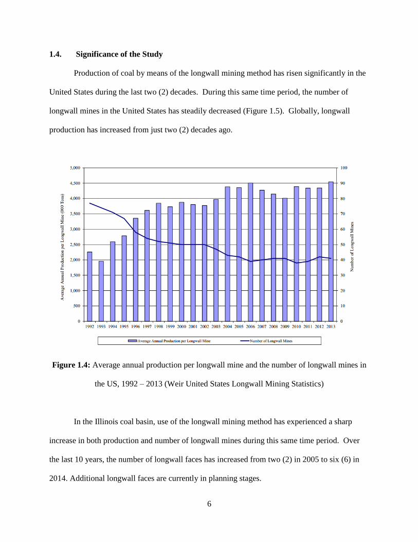
1.4. Significance of the Study

Production of coal by means of the longwall mining method has risen significantly in the

United States during the last two (2) decades. During this same time period, the number of

longwall mines in the United States has steadily decreased (Figure 1.5). Globally, longwall

production has increased from just two (2) decades ago.

Figure 1.4: Average annual production per longwall mine and the number of longwall mines in

the US, 1992 – 2013 (Weir United States Longwall Mining Statistics)

In the Illinois coal basin, use of the longwall mining method has experienced a sharp

increase in both production and number of longwall mines during this same time period. Over

the last 10 years, the number of longwall faces has increased from two (2) in 2005 to six (6) in

2014. Additional longwall faces are currently in planning stages.

7

Increasing application has resulted in greater potential for ground control problems while

crossing faults. Problems involving ground control include roof falls, rib sloughing, and floor

heave; all of which are related to stresses and displacements. Stress redistributions, inherent

mechanical properties of unique strata, and geological structures such as faults are principal

sources for issues involved with ground control. Ground control requires selecting and

maintaining face supports as well as primary, secondary, and supplemental supports in gate

development entries. Supplemental support design requirements and the timing of their

installation are important considerations when crossing faults. The analysis of conditions around

faulted longwall mining areas that is presented in this thesis can be used by mining companies

and other researchers to develop solutions for improved safety and productivity when such

conditions are encountered.

1.5. Thesis Structure

Chapter 2 reviews relevant literature to establish tasks for achieving research objectives.

This includes reviewing previous research on engineering rock mass properties used as input for

three-dimensional numerical modeling. Geological Strength Index (GSI) estimates and their

relationships to Hoek-Brown rock mass strength estimates are also reviewed.

Chapter 3 describes the two (2) different numerical models of mine workings that were

developed for analysis. They are: 1) A base model (Model 1) of a longwall panel’s set-up rooms

and gate development entries without faulting, and 2) A second model (Model 2) of the same

mine workings with a fault running through set-up rooms and gate development entries

(simulating the physical geometry of a fault in a case study mine). Non-linear modeling

incorporating a fault could not be achieved due to time-run requirements. The fault was modeled

8

in FLAC3D as a Ubiquitous Jointed Rock Mass (UJRM) plane. Linear models were run and

validated based on in-field studies and measurements at the case study mine site together with

previous and ongoing research conducted by ground control research at Southern Illinois

University Carbondale.

Chapter 4 explains analytical studies that evaluate stress and displacement redistribution

in both models as the longwall face advanced in 6-foot (2 m) increments through a distance of

1005 feet (324 m). Analyses were performed along several different cross-sections within each

model to assess effects of the fault on face supports and to formulate recommendations for

improved mining operations and secondary and supplemental supports.

Chapter 5 provides a summary of the research including both analytical studies and

modeling results. Recommendations for continuing this research are also presented.

9

CHAPTER 2

LITERATURE REVIEW

2.1. Overview of the Longwall Mining Method

There are two (2) primary extraction methods used in modern coal mines. The most

common method since the mid-1900s has been the room-and-pillar mining method. This system

requires coal to be extracted in multiple entries (rooms) that intersect with each other at right or

near right angles to create networks of openings (Figure 2.1). Coal extraction is performed by a

continuous miner. Entries are kept open with roof bolts as primary supports. These rooms are

also stabilized by un-mined columns of coal, termed pillars, which are left in place between

rooms. A room-and-pillar mine achieves extraction ratios of 40-50% in areas that are expected

to stay stable over long periods of time. In areas of the mine primarily focused on production that

will be sealed after mining, higher extraction ratios of 55-65% are achieved with different sized

pillars in different areas.

The second prominent mining method is known as longwall mining. A block of coal

between 1,000 and 1,500 feet (305-457 m) wide (Figure 2.1) is mined in slices of 3 feet (1 m) by

a shearer with roof strata caving behind face support structures into the mined-out area. The

length of the coal block (panel) varies from 10,000 to 15,000 feet (3050 to 4570 m). This mining

system enables 100% extraction of coal within the longwall panel. In the United States (US),

continual development and innovation of the longwall mining method since the early 1970s has

increased production tonnages and led to reductions in operational costs on a per ton basis.

However, longwall mining still requires large capital expenditures, long development times, a

large contiguous mining area, flat or slightly dipping seams, and uniform coal seam thickness.

10

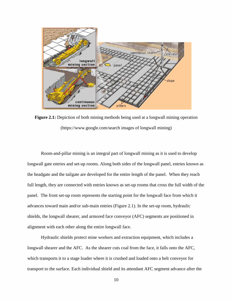
Figure 2.1: Depiction of both mining methods being used at a longwall mining operation

(https://www.google.com/search images of longwall mining)

Room-and-pillar mining is an integral part of longwall mining as it is used to develop

longwall gate entries and set-up rooms. Along both sides of the longwall panel, entries known as

the headgate and the tailgate are developed for the entire length of the panel. When they reach

full length, they are connected with entries known as set-up rooms that cross the full width of the

panel. The front set-up room represents the starting point for the longwall face from which it

advances toward main and/or sub-main entries (Figure 2.1). In the set-up room, hydraulic

shields, the longwall shearer, and armored face conveyor (AFC) segments are positioned in

alignment with each other along the entire longwall face.

Hydraulic shields protect mine workers and extraction equipment, which includes a

longwall shearer and the AFC. As the shearer cuts coal from the face, it falls onto the AFC,

which transports it to a stage loader where it is crushed and loaded onto a belt conveyor for

transport to the surface. Each individual shield and its attendant AFC segment advance after the

11

shearer passes by on each cut. Once the shearer is a reasonable distance past a given shield, the

shield pushes the AFC forward. Then the shield’s hydraulic main jacks disengage releasing

pressure on the roof. This allows the shield to pull itself forward by means of another hydraulic

jack connected to the AFC.

If the mining direction is from the set-up room towards main entries, it is considered to

be retreat longwall mining. With this approach, workers are always in a stable geological

environment. In other countries, advance longwall mining has been practiced where the face

starts at a point close to the main entries and mines toward the furthest extent of the coal block.

In this method, gate entries and the longwall panel are mined simultaneously.

As the longwall face advances, no support remains for the overlying rock that was once

above the coal seam. This lack of support results in the failure and ultimate caving of the roof

material. Caving of immediate roof strata continues until the geological structural system

stabilizes by reaching a new equilibrium. This caved material has a larger volume and different

physical properties than the intact rock. Failure of the overlying rock mass results in vertical

overburden loads transferring onto surrounding areas of higher stiffness, which includes solid

coal ahead of the face, development pillars in headgate and tailgate entries, and compacted caved

strata behind the face. The region of caved material is termed the “gob.”

2.2. Ground Control around Longwall Mining Areas

The longwall mining system is extremely complex in terms of structural mechanics and

involves significant stress redistributions when coal is mined. The system is dynamic during

longwall face retreat with interactions occurring among high stiffness areas, such as solid coal

ahead of the face and solid coal in development entry pillars, and relatively low stiffness areas

such as shield supports in the face area and gob behind the face. These interactions result in high

12

stress concentrations at different locations around the mining area including set-up rooms, pillars

in both headgate and tailgate development entries adjacent to the panel, and along the mining

face (Figure 2.2). These high stress concentrations are called abutment loads. Distribution of

loading around a longwall panel along cross-sections a-a, b-b, and c-c are shown in the figure

and will be discussed in the following sections. The intensity of these abutment loads is

dependent upon caving of the immediate roof and the vertical load carried by it as it gets

compacted. Low stiffness gob areas do not carry much load, but as the gob is compacted, it can

carry greater loads.

2.2.1. Gate Entries

As the solid coal is extracted, stresses are transferred onto gate entry pillars adjacent to

the panel. These load transfers result in stress concentrations around mined-out regions and are

referred to as abutment loading (Figure 2.2). The increased abutment loading, while extending

to the second-row gate pillars, has substantially greater loading on the first row. The distance the

abutment loading extends is defined by the equation (Peng and Chiang 1984):

𝐷 = 9.3√𝐻 (Eq. 2.1)

where D is horizontal distance affected by abutment loading (in feet), and

H is mining depth (in feet).

When evaluating stability of a longwall panel, T-junctions are of interest. T-junctions are

the connection between gate (head or tail) entries (forming the side boundaries of the longwall

panel) and the set-up rooms (forming the longwall face). As longwall mining commences in a

panel, abutment loads that form in the set-up rooms and the adjacent gate entries cause a peak

concentration of stresses in T-junction pillars. Another area of peak concentration will form in

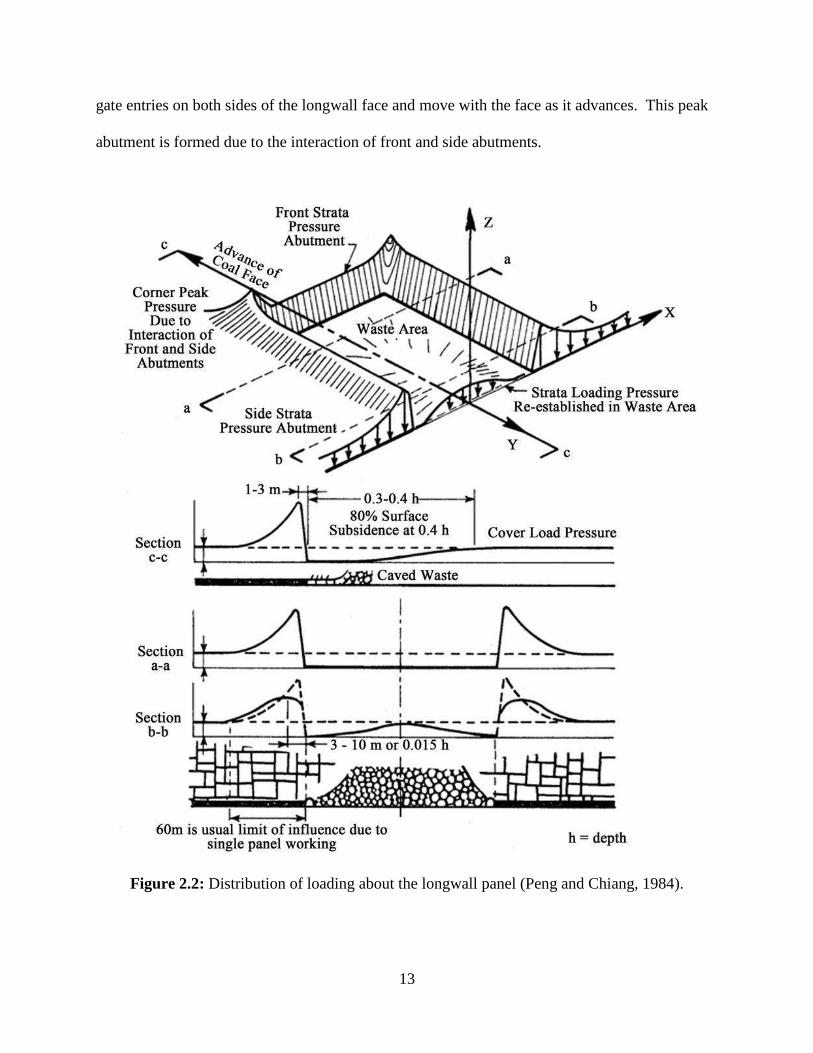
13

gate entries on both sides of the longwall face and move with the face as it advances. This peak

abutment is formed due to the interaction of front and side abutments.

Figure 2.2: Distribution of loading about the longwall panel (Peng and Chiang, 1984).

14

2.2.2. Face Area

Ground control in the face area is critical to a productive longwall face. Stresses on

longwall shields must remain within allowable limits to assure safety of workers and equipment.

This area is of concern when mining around or through geological anomalies such as fault zones

or dikes. These can significantly affect stress redistributions and displacements that occur.

Slippage along a shear plane results in high displacements at the location where the face

intersects a fault or dike zone and could potentially cause intense stress levels around the zone.

The intensity of stress redistributions and displacements depends upon the angle of dip of the

shear plane, the orientation of the shear plane with respect to the face, the curvilinear surface of

the fault zone, and engineering properties of the material along the shear plane. An evaluation of

the structural stability requires knowledge of these rock mass engineering properties.

As the longwall face advances, the immediate roof strata tend to fracture and fall into the

mined-out area behind the face (Figure 2.3). Yielding or brittle fracturing also occurs ahead of

the face as the coal is stiff enough for an abutment to form. Caving is a critical structural

element of the longwall face, as it reduces pressures on shield supports in the face area and ahead

of the face and allows gob to further compact and eventually take on some of the redistributed

load. Studies by Deb et al. (2006), Trueman et al. (2011), and Medhurst and Reed (2005) show

increased loading on shields near the center of the panel, with shields nearer to gate entries

sharing abutment loading with pillars in those development entries.

15

Figure 2.3: Caving and displacement of roof strata due to longwall face advance

(Kolebaevna, 1968).

2.2.3 Gob Area

As mining progresses, abutment zones form around and adjacent to the gob area.

Eventually, this caved gob material compacts to a point that it can carry load equal to pre-mining

load (Figure 2.2 section c-c). Caving in longwall mining is dependent upon tensile and shear

strength of caving materials. Since geology of the immediate roof and floor strata is highly

variable in thickness and stiffness, caving of roof strata is generally non-uniform and occurs in

zones (Figure 2.4). In regions where roof strata are thick, stiff, or of relatively high strength, it

becomes difficult to induce caving at a desired distance behind the longwall face. Large blocks

of hanging rock mass create a cantilever beam over longwall hydraulic shields in the face area

and increase stresses in those areas (Figure 1.2). Increased stresses in these areas can result in

productivity losses and potential damage to production equipment.

16

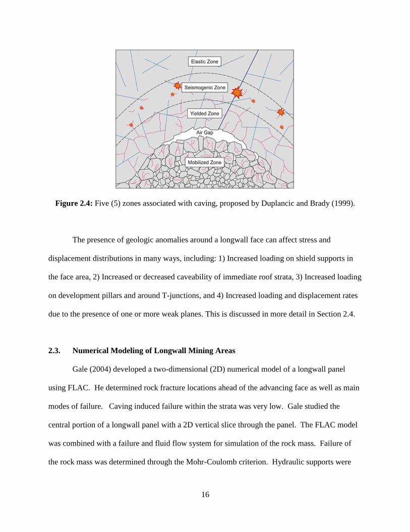
Figure 2.4: Five (5) zones associated with caving, proposed by Duplancic and Brady (1999).

The presence of geologic anomalies around a longwall face can affect stress and

displacement distributions in many ways, including: 1) Increased loading on shield supports in

the face area, 2) Increased or decreased caveability of immediate roof strata, 3) Increased loading

on development pillars and around T-junctions, and 4) Increased loading and displacement rates

due to the presence of one or more weak planes. This is discussed in more detail in Section 2.4.

2.3. Numerical Modeling of Longwall Mining Areas

Gale (2004) developed a two-dimensional (2D) numerical model of a longwall panel

using FLAC. He determined rock fracture locations ahead of the advancing face as well as main

modes of failure. Caving induced failure within the strata was very low. Gale studied the

central portion of a longwall panel with a 2D vertical slice through the panel. The FLAC model

was combined with a failure and fluid flow system for simulation of the rock mass. Failure of

the rock mass was determined through the Mohr-Coulomb criterion. Hydraulic supports were

17

simulated by adding a hydraulic set and yield function into the model along the simulated face.

Vertical loading was transferred through the shields by the inclusion of a canopy and base within

the simulation. Longwall mining was simulated by gradually advancing the shield simulation in

3-foot (1 m) increments once the model removed that amount of coal ahead of the face. Creation

of gob material was determined by both consolidation stiffness and post-failure criteria.

Verma and Deb (2008) used 2D plane strain in finite element models with a complete

factorial design of six (6) factors in ANSYS to analyze interactions between hydraulic supports

and surrounding strata for potential future deep longwall panels in India. These factors include

mining depth, immediate roof modulus, immediate roof thickness, shield capacity, immediate

roof friction angle, and whether the coal is hard or soft. Input values came from borehole

samples collected across India. The yield criterion used was a three-dimensional (3D) pressure-

dependent model, which estimates ultimate strength once a certain state of stress is reached. This

work led to the development of statistical predictions for leg pressure, roof-to-floor convergence,

and peak abutment loadings given the six (6) input factors.

Ozbay and Rozgonyi (2003) numerically modeled a 2-entry deep longwall system with

FLAC. To model the coal accurately, they created an initial model of a quarter coal pillar

(utilizing symmetry) and compared results to empirical formulas from Salamon and Munro

(1967) and Bieniawski (1984). Coal element engineering property inputs were modified within

the initial model until empirical formulas were well-reflected, then engineering inputs were

placed within the full longwall model. In the analysis, they compared the Mohr-Coulomb failure

criterion and the Mohr-Coulomb strain-softening criterion with field results. The strain-

softening behavior more accurately matched field results. The model excavated coal in

perimeter sections and then in longwall cuts allowing the model to equalize after each cut before

18

advancing again. Gob material was based on a ‘compaction model’ (Salamon, 1991) with non-

linear elastic behavior where vertical stress rises exponentially with increasing strain.

Vakili et al. (2010) compared results of a finite difference model in FLAC3D and a

Boundary Element model within MAP3D to the amount of surface subsidence and pillar stress

expected within a typical longwall mining environment. Linear elastic modeling is preferred

within MAP3D, so models studied within the software included either a gob material substitute

or no gob material at all. The model with no gob material was the outlier of the MAP3D models.

MAP3D was determined to be an acceptable modeling approach for the large-scale longwall

environment, but has significant limitations for caving. An additional material to act as gob is

not a necessity within FLAC3D. The study determined that, although FLAC3D requires more

operator training, it is better suited for modeling environments where it is difficult to obtain in

situ caving measurements (i.e., stress levels within caved medium).

Shabanimashcool and Li (2012) evaluated the stability of gate entries in a Norwegian

longwall coal mine using FLAC3D to create a numerical model. The rock mass in the numerical

model undergoes strain-softening such that fracturing material undergoes unloading and

reloading. Caved material consolidation is represented by the Double-Yield (DY) Constitutive

Model within FLAC3D. The longwall is advanced in 16-foot (5-m) intervals. An algorithm was

created to determine the thickness of the cave-in roof for the caving process behind the

advancing longwall face. Empirical results show roof strata in gate entries are more affected by

development of gate entries than by the active longwall mining process.

2.3.1 Development of Rock Mass Properties for Modeling

Solid earth material containing bedding planes, layered strata, and discontinuities such as

joints, dikes, faults, shear zones, etc., is referred to as rock mass. Laboratory-determined

19

engineering properties for intact rock cores do not accurately represent rock mass values since

they do not incorporate the complexity of the physical environment. Intact rock may behave

isotropically or anisotropic orthotropically, depending upon the rock sample. However, a rock

mass would be expected to have anisotropic properties. Rock mass engineering properties must

be assessed as accurately as possible to analyze stability of jointed rock mass.

2.3.2 Intact Rock and Rock Mass Mechanical Behavior

An intact rock will not have fissures or joints within it. Strength behavior of intact rock

is determined through strength tests in tension, shear, and compression loading at different

confining stresses. Intact rock can refer to a lab specimen without discontinuities or an

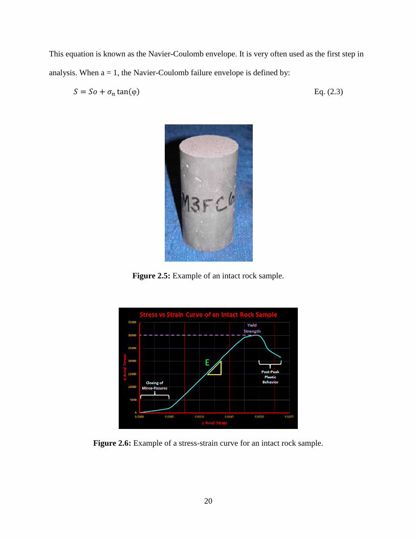
individual block of the rock mass (Figure 2.5). Examples of test results are given in Figure 2.6.

Samples in an unconfined environment typically fail in a brittle manner with sudden loss of load

carrying capacity (Figure 2.7). At higher confining stresses, the failure behavior shows a more

gradual loss of load carrying capacity, and in some strain-hardening cases, even increased load

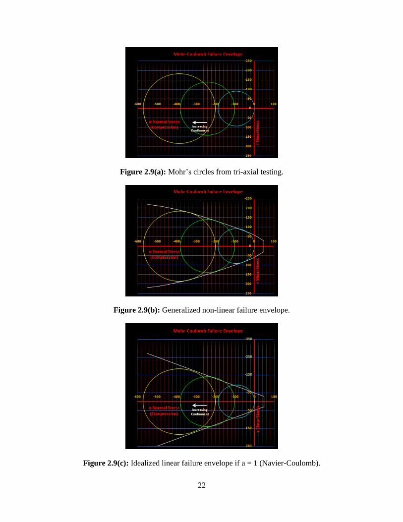
carrying capacity (Figure 2.8). The failure behavior may be depicted as a failure envelope using

the Mohr’s circle approach shown in Figure 2.9(a). Connecting multiple circles with a tangent

line represents the failure envelope. This generalized non-linear envelope (Figure 2.9(b)) can be

idealized as a linear envelope (Figure 2.9(c)) with Equation 2.2:

𝑆 = 𝑆𝑜 + [𝜎𝑛 tan(φ)]𝑎 Eq. (2.2)

where S is the shear strength on a particular plane within a material,

𝜎𝑛 is the normal stress acting on the plane,

φ represents the angle of internal friction of the material, and

𝑆𝑜 represents the cohesion of the material.

20

This equation is known as the Navier-Coulomb envelope. It is very often used as the first step in

analysis. When a = 1, the Navier-Coulomb failure envelope is defined by:

𝑆 = 𝑆𝑜 + 𝜎𝑛 tan(φ) Eq. (2.3)

Figure 2.5: Example of an intact rock sample.

Figure 2.6: Example of a stress-strain curve for an intact rock sample.

21

Figure 2.7: Stress-strain curve for a brittle material.

Figure 2.8: Stress strain curve for strain-hardening (upper) and strain-softening (lower) material.

22

Figure 2.9(a): Mohr’s circles from tri-axial testing.

Figure 2.9(b): Generalized non-linear failure envelope.

Figure 2.9(c): Idealized linear failure envelope if a = 1 (Navier-Coulomb).

23

To develop ground control practices that preserve stability in a jointed rock mass being

mined, it is crucial to be as accurate as is possible in the determination of its mechanical

properties. However, values for mechanical properties obtained through experimentation on

intact rock samples are not always representative of the rock mass from whence they came.

Because of scale and the sampling process used to obtain them, individual intact rock samples do

not have the jointing seen in rock masses as a whole. Intact rock samples tend to behave

mechanically in isotropic or orthotropic manners depending upon the rock sample whereas a

rock mass may behave in more of an anisotropic fashion.

After intact rock properties are determined, that information can be used to estimate rock

mass properties. The Geological Strength Index (GSI) is a crucial tool for this estimation (Hoek

et al., 2005). Combined with intact rock engineering properties, the GSI enables approximation

of the rock mass’ Young’s modulus, Poisson’s ratio, as well as the rock mass yielding curve.

The procedure for estimating rock mass behavior is discussed in depth in Chapter 3.

2.3.3 Hoek-Brown Failure Criterion

Unlike the Navier-Coulomb failure envelope, this criterion’s yield surface is non-linear

and can account for the decreasing incremental gain of strength with additional confinement

(Figure 2.10). Its equation is given below:

𝜎1′ = 𝜎3

′ + 𝜎𝑐𝑖(𝑚𝜎3

′

𝜎𝑐𝑖+ 𝑠)𝑎 Eq. (2.4)

where 𝜎1′ and 𝜎3

′ are major and minor effective principal stresses on the failure plane,

𝜎𝑐𝑖 is the uni-axial compressive strength for intact rock, and

m and s are material constants that are both dependent upon the GSI value.

24

Figure 2.10: Hoek-Brown failure envelope for rock mass strength (σ1 and σ3 planes).

To obtain accurate values for use within the model, it is important to first develop inputs

for the Hoek-Brown failure criterion that accurately depict non-linearity to appropriately account

for the discontinuous nature of the rock mass. The yield surface for Hoek-Brown is dependent

upon the GSI value, the disturbance factor D, the mi value, and uni-axial compressive strength

(UCS) parameters. The disturbance factor only comes into consideration when unnatural

processes, such as drilling and blasting for tunneling, have been conducted. For this study, the

disturbance factor is set to zero, since no blasting is involved. Displacements within the rock

mass are in part derived from Young’s modulus for intact rock using samples representative of

the various types of strata in the mining environment. The GSI value is obtained by evaluating

the lithology within the rock mass with respect to its structure and the surface weathering

conditions of rock samples taken from the rock mass (Hoek et al., 2005). This value ranges from

0 for extremely weathered and deformed geologic structures, to 100 for un-weathered and thick

sedimentary beds (Table 2.1).

25

The Hoek-Brown criterion has an input, mi, called the material constant (Hoek et al.

2002), which corresponds with the friction strength of the rock mass. Modifying this value to a

lower amount will reduce the curvature of the Hoek-Brown failure envelope. The curve fitting

parameter mi can be accurately approximated by conducting tri-axial tests on the intact rock

sample. This is in addition to the compressive strength value obtained through a series of UCS

tests conducted on intact rock samples.

Table 2.1: Common GSI ranges for typical rock formations (Marinos and Hoek, 2000).

Rock Type GSI value Consideration

Sandstones • Typical formation

(45-90)

• Tectonically brecciated

(30-45)

• If weak interlayers, such as clayey or

gypsiferous cement, are involved, GSI values

may lower.

Silstones,

clayshales

• Bedded, foliated,

fractured (45-20)

• Sheared, brecciated

(25-5)

• GSI is not applicable in homogeneous rock

with no formation of discontinuities.

• If they are present as thin interlayers between

stronger rocks, a downgrading of the rock

mass towards the right part of the chart

should be considered.

Limestones • Massive (90-45)

• Thin bedded (55-35)

• Brecciated (45-30)

• During folding thin bedded layers result in

differential movement lowering the GSI.

It is imperative for geotechnical analysis to ascertain mechanical parameters for the rock

mass so that modeling behavior reflects what is observed in the mining environment. The key

input parameters required to correctly model a longwall environment numerically include GSI,

mi (intrinsic material property), UCS of intact rock, elastic moduli, and Hoek-Brown residual

parameters. The intrinsic heterogeneous distribution of discontinuities within the rock mass

makes it difficult to determine these parameters. Mechanical properties of the rock mass for this

26

study were determined from laboratory testing on core samples, tests in the field, visual

observations, and past experience. Testing on samples of caved material is impractical and

unfeasible. Validating correct parameter values was performed by comparing model results to

those ascertained in the field.

2.3.4. Mohr-Coulomb Failure Criterion for Intact Rock

For this study, tension will be treated as positive and the relationship between principal

stresses will be: σ1 ≥ σ2 ≥ σ3 . This criterion is specifically for brittle materials under

compression, such as rock and concrete. A Mohr-Coulomb analysis examines the state of stress

along mutually orthogonal planes and analyzes every possible rotation of those planes to

estimate if failure may occur within the material. Every possible orientation can be plotted in 3D

space or in 2D with each plane represented by an individual Mohr’s circle (Figure 2.11).

Figure 2.11: Envelope in Mohr-space using σ1 and σ3 planes.

27

The angle of internal friction and cohesion inputs are required for the development of a

linear yield surface that is dependent upon confining pressure. If the yield surface, termed the

failure envelope, is breached, then the material is expected to fail in the shear mode. However,

tension failure is possible if the region of the failure envelope termed the tension cut-off is

breached. The location where the failure envelope is breached by a state of stress can be related

to the location and/or orientation of a failure surface in an intact rock given the orientation of

stresses applied on the rock. At higher confining pressures, the angle of internal friction is seen

to decrease during experiments, but the criterion sets the angle as a constant. The vertical axis

intercept is the location of no confinement and is defined as the cohesion of the material. The

angle of internal friction determines the steepness of the linear yield surface. If the angle of

internal friction is non-zero, the material will be assumed to gain strength through additional

confinement. When unconfined, the material can only fail if its cohesion is surpassed.

2.4. Stress Redistribution and Mechanisms of Failure

A dynamic mining environment with changing geometries will result in redistributions of

stress fields. During mining of headgate and tailgate development entries, rock once acting as

confining material is removed. Without this confinement, the stiffness of the rock immediately

surrounding these entries is reduced and loading in these areas will redistribute to stiffer, more

confined rock masses. Through this redistribution, parts of the rock mass surrounding the entry

may experience tension depending upon the magnitude and orientations of principal stress fields

and the orientation of entries. Failure in rocks will occur either in tensile or shearing modes. If

the difference in principal stresses becomes great enough, then failure in the shear mode is

possible depending on the greatest principal stress.

28

2.5. Numerical Modeling of Geologic Anomalies and Faults in Longwall Mining

A rock mass has numerous discontinuities including sets of joints, bedding planes

resulting from sedimentary deposition, and in some instances, major shear planes. Behavior of a

rock mass differs from intact rock in how deformation occurs. Intact rock deforms through strain

and shape distortion. A rock mass, on the other hand, can deform in the same manner, but also

through movement along numerous discontinuous surfaces where sliding could occur. To

account for this behavior, ubiquitous joints can be included into models, particularly for linear

features such as fault planes.

Ubiquitous Joint Rock Mass (UJRM) is a methodology for applying a weak plane or

discontinuity to a rock mass simulated by a continuum in numerical modeling. UJRM weak

plane mechanics is defined by the Mohr-Coulomb failure criterion with the tension cutoff along a

weak plane (ITASCA, 2012). Many previous researchers have employed and verified this

technique, including Lietner et al. (2006), Sainsbury et al. (2008), Sainsbury and Sainsbury

(2017), Clark (2006), Board et al. (1996), and Chiu et al. (2013). While this methodology

presents a highly useful tool, it also has limitations that must be considered. There are several

important joints-related factors that UJRM does not consider including joint spacing, stiffness,

and geometry (Sainsbury 2012). Implementation of a ubiquitous joint plane or surface in finite

element models requires six (6) inputs: strike, dip, dilation, cohesion, friction angle, and tensile

strength. To generate realistic modeling results, calibration of UJRM is usually required.

Geological discontinuities influence both failure initiation as well as progression.

Weakness planes along the discontinuity shape the extent of failures. It is critical that the panel

and entries within the panel be oriented with respect to the discontinuity and lateral stresses to

lower peak stress levels in the mining environment. Panel design must take into account

29

interactions between stresses, discontinuity surfaces, and the configuration of mining entries.

Stresses and deformation are also subject to variance in geo-mechanical properties of changing

strata and the failure of weaker lithologies such as coal and claystone.

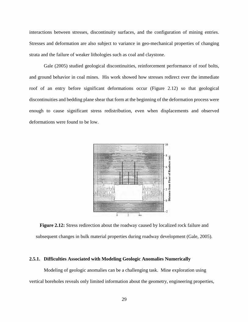
Gale (2005) studied geological discontinuities, reinforcement performance of roof bolts,

and ground behavior in coal mines. His work showed how stresses redirect over the immediate

roof of an entry before significant deformations occur (Figure 2.12) so that geological

discontinuities and bedding plane shear that form at the beginning of the deformation process were

enough to cause significant stress redistribution, even when displacements and observed

deformations were found to be low.

Figure 2.12: Stress redirection about the roadway caused by localized rock failure and

subsequent changes in bulk material properties during roadway development (Gale, 2005).

2.5.1. Difficulties Associated with Modeling Geologic Anomalies Numerically

Modeling of geologic anomalies can be a challenging task. Mine exploration using

vertical boreholes reveals only limited information about the geometry, engineering properties,

30

and anomalies within a given geology. Therefore, reasonable approximations must be made for

the location and extent of anomalies within a model. Modeling mechanical behavior of an

anomaly can be aided with information gathered from control points installed in active mining

environments. Differences in behavior between control points around geologic anomalies and

those in standard geologic areas show the influence and magnitude of an anomaly. This

comparative information helps to ensure that input parameters are within acceptable tolerances.

2.6. Fault Modeling Using UJRM Technique

Abbasi et al. (2014) developed analytical tools to quantify displacements around a fault

zone as a longwall face advanced towards it. They used FLAC3D software to generate a 3D

model of a southern Illinois longwall panel intersected by a fault zone. The fault zone was

simulated using the UJRM method. The model used the Hoek-Brown method with GSI inputs

for the failure criteria of the strata, and the Mohr-Coulomb failure criteria for the fault zone. GSI

estimates were used for different lithologic units to develop their rock mass engineering

properties that were used in numerical models. Caved gob material engineering behavior was

approximated by an empirically distributed loading function behind the advancing face. This

approach led to roof-to-floor convergence results in several areas that were only 15-20%

different than corresponding values measured in the field. Results showed that development

entries intersected by the fault start to experience the deformational effect of the fault when the

longwall face was 230 feet (70 m) away. Model observations were corroborated in the field

through convergence measurements. Supplementary roof supports were used in gate

development entries that allowed the company to mine successfully through the fault without

loss of production or accident.

31

2.7. Modeling of Caved Gob in Longwall Mining

Since the start of mining methods that employ caving, researchers have been attempting

to accurately predict caving behavior and propagation. Thin et al. (1993) used the DY model for

gob material. Within FLAC, the DY model uses a strain-stiffening relationship in the gob where

vertical stress within gob material is used to calculate a vertical strain. They found that the

thicker the overlying beds above the coal, the greater distance initial loading reaches into the

gob, and that this distance shortened with increasing depth.

Sainsbury (2010) created a numerical caving model with the Mohr-Coulomb failure

criteria. A fully fractured and bulked cave material was simulated in the undercut regions of the

numerical model. The study examined the sensitivity to caveability of the rock mass in the early

stages of production. The study found that increased bulking occurred at the edge of the caved

region, and that the rate of cave propagation increased with the depth of mining.

2.8. Experimental Approaches for Assessment of Caving

There are three (3) applicable methods that are useful in predicting caving behavior, each

with its own strengths and weaknesses, as discussed next. The research reported in this thesis

utilized all three (3) approaches.

2.8.1 Analytical Approach

It has been previously suggested by researchers that simplistic analytical volume

relationships could be utilized in estimating caved material bulking and caving propagation

(Beck et al., 2006). This approach makes the assumptions that propagation is in the vertical

direction, at a constant rate, and that initiation of caving will always occur.

32

The analytical approach has been found to be inaccurate (Sainsbury, 2012) possibly due

to geomechanical rock mass properties being ignored during calculations.

2.8.2 Empircal Approach

There have been several empirical approaches proposed to approximate caveability in the

mining environment. Laubscher (1994) worked on a collection of cases from past caving

practices in South Africa’s block-cave mining of kimberlite pipes. This work characterized the

extent of caving into three (3) distinct possibilities. Mining can result in: 1) no caving, 2) a

transitional state of caving whereby there is cave initiation, but a lack of significant cave

propagation, and 3) complete caving.

In more recent times, several researchers have obtained results that differ considerably

from data presented by Laubscher. Kimberlite pipes are a weaker rock originating from deep

subterranean eruptions, so data collected by Laubscher represented a weaker rock mass than is

generally found in mining environments. Research to predict caveability for harder rock masses

produced another prediction tool for caveability (Trueman et al.; 2003).

Both of these methods were developed based on collected sets of data, which causes

some limitations. They lack sufficient information to estimate both rates of caving and zones of

mechanical behavior in a caving environment.

2.8.3 Numerical Approach

Many numerical modeling techniques are available to researchers attempting to analyze

geotechnical environment. These techniques include Boundary Element, Distinct Element,

Finite Difference, Finite Element, and other numerical techniques that combine some or all of the

aforementioned techniques. While any analysis program can be used to examine the

33

geotechnical environment, the critical aspect of analysis is the methodology incorporated within

the study.

Geotechnical material presents researchers with a substantial challenge. Unlike man-

made materials that are manufactured, natural material is extraordinarily complex with micro-

fissures and varying arrangements of microscopic minerals. It is not possible using today’s

computers to model materials down to this scale while still trying to evaluate a macro-level

environment such as longwall mining. Therefore, approximations must be made by researchers

to define inputs such that reality is represented as well as possible. An international study on

caving environments by Pierce and Lorig (1998) illustrates an enhanced methodology whereby

sequential undercuts are simulated and a user-defined function can modify material properties

based on plasticity state and strain. By analyzing 3D states of stress that surround the undercut, a

point of self-sustaining instability can be determined.

34

CHAPTER 3

MODEL DEVELOPMENT AND FIELD MONITORING STUDIES

3.1 Description of Physical Problem and Mine Environment

The overarching purpose of this study is to apply analytical tools to quantify and determine

incremental stresses and deformations that occur around a fault as longwall mining progresses

toward, through, and away from it. Fault planes embody spatial discontinuities. They disturb the

surrounding rock mass causing it to degrade. Both the weak fault plane and the surrounding

degraded rock mass have different engineering properties than the adjoining undisturbed rock

mass. Areas around the fault can undergo large displacements relative to the rock mass with the

potential effect of shedding stresses onto the adjoining rock mass. Thus, when mining intersects

a fault plane, mine operators must be aware of an increase in loading on some portions of coal ribs

along an entry and on the caved or falling rock from the roof. The redistribution of stresses during

mining around fault zones has the potential to result in additional deformations, rigid-body

displacements, and rotations.

Another region of differing stiffness is the caved gob after longwall mining has removed

coal from an area. It is here that stress redistributions are caused by varying stiffnesses of the

spatially distributed gob area and by coal pillar failures. Displacements in these regions are

affected by the orientation of the fault, the extent of the disturbed rock mass, properties of the fault

plane, the dynamic stress field resulting from a retreating longwall face, properties of the spatially

distributed gob area, and soft floor material.

The case study developed in this thesis is for a mine in southeastern Illinois extracting coal

from the Herrin No. 6 coal seam at a depth of about 600 feet (180 m). The immediate roof

35

consisted of black shale, limestone, dark shale, coal riders, and sandy shale. The floor stratum is

weak claystone underlain by shale rock. The mine uses the longwall mining method with panels

generally oriented in the east-west direction. Gate entry widths are 19 feet (5.7 m) and crosscut

spacing (center-to-center distance) ranges from 100 to 140 feet (30 to 45 m). T-junction pillar

dimensions are 80 feet by 80 feet (24 m by 24 m).

The case study mine encountered both major and minor faults and grabens. Faults in the

study had a general strike and dip of N30°W and about 60°, respectively. Ground movement

monitoring points for the first fault zone encountered when mining gate entries are shown in Figure

3.1. A second fault zone was encountered as gate entry development continued. The main fault

had a down-throw displacement toward the east of 3 feet (1 m) as depicted in Figure 3.2. This

fault extended into the set-up rooms on the tailgate side.

(a) (b)

Figure 3.1: Fault and ground movement monitoring station locations in: (a) Headgate of case

study panel, and (b) Headgate of adjoining longwall panel for first fault zone.

36

(a) (b)

Figure 3.2: (a) Cross-sectional view of second fault/graben area in headgate return entry of case

study panel, and (b) Plan view of same area showing ground movement monitoring locations.

3.2 Identification of Modeling Areas

A plan view of the longwall panel’s set-up rooms, tailgate entries, and headgate entries is

shown in Figure 3.3 with pillar dimensions indicated. Designed pillar dimensions are

standardized at 80 feet (24 m), 120 feet (36 m), and 140 feet (42 m). Entries in set-up rooms and

headgate and tailgate sections are supported using 6-foot (1.8-m) long, #6 rebar, fully-grouted

passive bolts as primary support. Areas with highly variable roof lithologies use steel channels in

conjunction with fully grouted bolts. Set-up rooms use trusses as secondary support at 10-foot

(3-m) intervals. Mining thickness is about 6.0 feet (1.8 m).

37

Figure 3.3: Layout and dimensions of the modeled mining environment.

A plan view of the modeled region at the coal elevation is shown in Figure 3.4 with the

fault highlighted. The figure represents the modeled state immediately following development

of set-up rooms and gate entries. As can be seen, the fault intersects the longwall face from the

start of mining up to the fourth chain pillar in the headgate entry. Several gate entry pillars are

intercepted by the fault as well.

For the sake of computing efficiency, only the portion of the longwall panel intersected

by the fault was modeled. The other (symmetrical) half of the panel was not included. By

limiting focus on this region, the density of elements within the model could be increased.

Model boundaries were kept 150 feet (45 m) away from any entries so that intersections of fault

and entry would not be distorted by being located at the model boundary.

38

Figure 3.4: Area modeled at the coal seam level with fault zone highlighted.

3.2.1. Development of Numerical Models

Models were developed using FLAC3D, a structural analysis software developed by the

Itasca Consulting Group that is used extensively for geotechnical modeling of geologic problems

that involve highly complex geometries, and linear as well as non-linear behavior. FLAC3D is

based on the finite difference computational scheme. Two (2) separate models were developed:

Model 1 of mine workings without a fault, and Model 2 of mine workings with a fault. Both

models were analyzed using linear properties and rock mass properties computed from intact

rock properties using the well-established Hoek-Brown failure criterion (Hoek et al., 2002). The

fault was modeled as a Ubiquitous Jointed Rock Mass (UJRM) in a well-defined spatial plane

with weak rock mass surrounding the plane as discussed in Chapter 2 (Section 2.5).

39

3.2.2. Immediate Roof and Floor Lithology of Models

Each distinct geologic unit such as sandstone or limestone in the sedimentary deposit is

known as a lithologic unit. Attributes of each lithologic unit change spatially. It is impossible to

model continuous variability in these attributes. Therefore, average attributes of lithologic units

above and below the coal seam, and the coal seam itself, were modeled in a columnar section as

described in Table 3.1. The base of the model is 43 feet (13 m) of shale. Layers above this shale

from bottom to top are as follows:

• 3 feet (1 m) of weak limestone,

• 3 feet (1 m) of gray shale,

• 2 feet (0.7 m) of shale,

• 1 foot (0.3 m) of claystone,

• 6 feet (2 m) of coal,

• 2 feet (0.6 m) of black shale,

• 2 feet (0.6 m) of gray shale,

• 2 feet (0.7 m) of weak limestone,

• 3 feet (1 m) of weak shale, and

• 3 feet (1m) of limestone.

At the top of the model is 39 feet (12 m) of shale.

40

Table 3.1: Engineering properties of rock strata used in modeling.

3.3 Model and Engineering Properties Development

Two (2) models were generated for analysis. The difference between them was UJRM

inclusion. To estimate effects of UJRM zones on stress and displacement within a macro-

system, a base case without any discontinuities was needed. This base case model was termed

Model 1. Then, a second elastic model was created to be identical to the first, but with UJRM

zones included establishing the effect of a geological discontinuity. This model was termed

Model 2. A comparison of results from these two (2) elastic models is discussed in Chapter 4.

Uniform strata thickness was preserved for both models.

Strata Location (ft.) Location (m.) GSI mi Density (pcf) σci (psi) Ei (psi)

Shale 72 - 112 22 - 34 70 10 155 6000 500000

Good Limestone 69 - 72 21 - 22 95 15 165 12000 1326000

Weak Shale 66 - 69 20 - 21 65 9 150 5500 700000

Weak Limestone 63 - 66 19.3 - 20 80 13 160 7500 850000

Gray Shale 61 - 63 18.6 - 19.3 70 9 150 5500 750000

Black Shale 59 - 61 18 - 18.6 65 9 140 4000 650000

Coal 53 - 59 16 - 18 62 8 80 3500 400000

Clay Stone 52 - 53 15.7 - 16 58 50 135 1200 250000

Shale 50 - 52 15 - 15.7 70 10 155 6000 500000

Gray Shale 46 - 50 14 - 15 70 9 150 5500 750000

Weak Limestone 43 - 46 13 - 14 80 13 160 7500 850000

Shale 0 - 43 0 - 13 70 10 155 6000 500000

Strata Erm (psi) mb s a v σc (psi) σ'3n (psi) Φ' c' (psi) Bulk Modulus, K (psi) Shear Modulus, G (psi)

Shale 367000 3.4 0.036 0.501 0.215 1130 0.00006 32.1 570 215000 151000

Good Limestone 1299000 12.5 0.574 0.5 0.1775 9080 0.00003 47.5 1710 672000 551000

Weak Shale 443000 2.6 0.02 0.502 0.2225 780 0.00007 29.1 490 265000 181000

Weak Limestone 748000 6.4 0.108 0.501 0.2 2470 0.00005 39.1 810 416000 312000

Gray Shale 550000 3.1 0.036 0.501 0.215 1030 0.00007 30.5 540 322000 226000

Black Shale 410000 2.6 0.02 0.502 0.2225 570 0.00009 26.6 430 247000 168000

Coal 226000 2.1 0.015 0.502 0.227 420 0.0001 23.8 380 138000 93000

Clay Stone 118000 11.2 0.009 0.503 0.233 120 0.0003 29 460 74000 48000

Shale 367000 3.4 0.036 0.501 0.215 1130 0.00006 32.1 570 215000 151000

Gray Shale 550000 3.1 0.036 0.501 0.215 1030 0.00007 30.5 540 322000 226000

Weak Limestone 748000 6.4 0.108 0.501 0.2 2470 0.00005 39.1 810 416000 312000

Shale 367000 3.4 0.036 0.501 0.215 1130 0.00006 32.1 570 215000 151000

Strata Erm (psi) mb v σc (psi) σ'3n (psi) Φ' c' (psi)

Shale 183000 1.9 0.2405 440 0.00006 27.3 430

Good Limestone 996000 5.3 0.2135 2380 0.00003 41.7 840

Weak Shale 202000 1.5 0.2465 320 0.00007 24.7 380

Weak Limestone 442000 3.1 0.23 800 0.00005 33.3 570

Gray Shale 275000 1.7 0.2405 390 0.00007 25.8 410

Black Shale 188000 1.5 0.2465 230 0.00009 22.3 340

Coal 102000 1.2 0.2495 170 0.0001 20 3000

Clay Stone 52000 6.8 0.254 60 0.0003 25.3 380

Shale 183000 1.9 0.2405 440 0.00006 27.3 430

Gray Shale 275000 1.7 0.2405 390 0.00007 25.8 410

Weak Limestone 442000 3.1 0.23 800 0.00005 33.3 570

Shale 183000 1.9 0.2405 440 0.00006 27.3 430

Bulk Modulus, K (psi)

Stra

ta, I

nta

ct R

ock

Val

ues

, an

d G

SI In

pu

tsD

eriv

ed R

ock

Mas

s P

rop

erti

es

217000

259000

217000

217000

33000

139000

194000

217000

259000

83000

365000

217000

118000

178000

118000

118000

57000

11000

Shear Modulus, G (psi)

146000

118000

178000

28000

297000

118000

0.003 0.506

Ub

iqu

ito

us

Join

t R

ock

Mas

s P

rop

erti

es

0.005 0.505

0.04 0.501

0.003

s a

0.506

0.012 0.503

0.005 0.505

0.003 0.507

0.002 0.509

0.005 0.505

0.005 0.505

0.012 0.503

0.005 0.505

41

3.3.1 Model Size

Both models were 1640 feet (500 m) long, 1640 feet (500 m) wide, and 110 feet (34 m)

high. Lithological units 50 feet (15 m) above and 50 feet (15 m) below the coal seam were

modeled to allow a reasonable distance for stress redistributions to equilibrate. A uniform

vertical stress of 550 psi (3.8 MPa) was applied on the upper boundary of the model to simulate

the remaining overburden. This was necessary to allow for large face advance distances and

adequate solid coal on model peripheries so that stress levels would return to their virgin state.

Elements created in both models were a uniform 6-foot ⨯ 6-foot (2-m ⨯ 2-m) size horizontally,

but varied in thickness vertically. Weak claystone floor elements were 1 foot (0.3 m) in

thickness. Coal seam elements were 1.5 feet (0.5 m) in thickness. Black shale in the immediate

roof was 2 feet (0.6 m) in vertical thickness. Models were constructed to be rectangular prisms

250 elements long, 250 elements wide, and 38 elements thick for a total of 2,375,000 elements.

An interface was included between the claystone unit and the coal layer to prevent

elements in the immediate roof layer above the coal seam from penetrating elements into the coal

seam floor. When coal elements are removed (i.e., simulating mining), the roof deforms towards

the floor and there must be an impermeable barrier to keep roof elements from penetrating into

the floor. This interface was assigned properties to prevent penetration of the roof and floor

elements, but to minimize it interfering with gob loading behavior. Interface properties had to be

calibrated via an iterative process to achieve this balance.

3.3.2 Engineering Properties of Intact Rocks

The engineering properties used during this study were derived from experience and a

previous study at the cooperating mine by Chugh et al. (2013). The previous study examined the

42

properties of strata at and around the fault zone. Bulk samples and cores were tested and average

property values for the strata were determined.

3.3.3 Additional Engineering Properties

Elastic engineering properties, such as Geological Strength Index (GSI), material

constant mi, intact rock uni-axial compressive strength σci, and intact rock Young’s modulus Ei,

for different lithologic units contained in the modeled rock mass are given in Table 3.1. These

were based on previous studies conducted at Southern Illinois University Carbondale at the

cooperating mine.

Development of Hoek-Brown rock mass parameters for non-linear analysis was more

complex. Hoek-Brown failure criterion relates principal stresses σ1 and σ3 (Equation 3.1). These

were calculated from estimated values of the GSI for each lithologic unit.

The rock mass Young’s modulus for each layer was developed using Equation 3.2. In

this equation, D, the disturbance factor, was always assigned a value of 0, as it applies generally

to blasted rock. Rock mass elastic modulus and Poisson’s ratio estimates were used to calculate

rock mass bulk and shear moduli. Material constants mb, s, and a, can be calculated from

Equations 3.3, 3.4, and 3.5, which are based on the GSI value. Poisson’s ratio for each strata

was calculated from Equation 3.6.

Most researchers are more familiar with the Mohr-Coulomb failure criterion, which

relates normal stress and shear stress on a plane. To approximate the equivalent Mohr-Coulomb

cohesion and angle of internal friction values, it is important to first know the value for σ3nor the

confining stress. Equation 3.7 is used to determine this value. It is dependent upon the value

σ’3max, where σ’3maxis the highest confining stress for which Hoek-Brown and Mohr-Coulomb

43

relationships are to be examined. A value of 2500 psi (17 MPa) was chosen for σ’3max. This is a

vertical stress concentration factor of 4.5, which is unlikely to be achieved except for at the

corner of pillars. Obtaining the equivalent Mohr-Coulomb relationship over the span of σ’3max

for each lithologic unit requires constants mb, s, and a, as well as the intact strength of

material,σ’ci, and the value of σ3n. The complex equations for cohesion and angle of internal

friction are shown in Equations 3.8 and 3.9.

σ1 = σ3 + Co(mbσ3

Co+ S)a Eq. (3.1)

Erm = Ei (0.02 +1−D/2

1+𝑒(

60+15𝐷−𝐺𝑆𝐼11 )

) Eq. (3.2)

mb = mi exp (GSI−100

28−14D) Eq. (3.3)

s = exp (GSI−100

9−3D) Eq. (3.4)

a =1

2+

1

6(e−

GSI

15 + e−20

3 ) Eq. (3.5)

v = 0.32 − 0.0015xGSI Eq. (3.6)

σ3n =σ′

3max

σci Eq. (3.7)

Eq. (3.8)

Eq. (3.9)

44

3.3.4 Development of Strata Properties Along the Fault

As previously mentioned, the fault was modeled as a UJRM plane. This plane was

developed with a dip of approximately 35 degrees off the horizontal. The dip went downward

along the positive y-direction and negative x-direction. FLAC3D allows estimated engineering

properties of the fault to be assigned not only to the UJRM plane, but also to the rock mass

adjoining the fault plane defined by the user. Engineering properties along the UJRM and

adjoining the UJRM for different lithologic units were developed in the manner described

previously. The same method and values were applied, and except for the GSI value, all other

constants were preserved. The GSI value of each lithologic unit was reduced to represent the

weaker material along the fault plane. UJRM zones within models were approximately 10 feet

(3 m) in width.

3.3.5 Modeling of Face Advance

Coal seam elements were always 6-ft ⨯ 6-ft (2-m ⨯ 2-m) in the horizontal plane. The

longwall shearer extracts a slice of approximately 3 feet (1 m) in horizontal thickness when

making a cut along the face. Given the element size chosen in modeling, face advance was

simulated in 6-ft (2-m) increments. In numerical modeling, each simulated advance involved

removing a full row of elements and running the simulation again until equilibrium was achieved

and resulting data saved. This process of modeling face advance in 6-ft (2-m) increments was

repeated through a total advance of 1063 feet (324 m) in the FISH (short for “FLAC-ISH” or the

language of FLAC) code. Vertical forces within the face area (i.e., simulating longwall shield

supports) were also moved with face advance after each cut was completed. The move distance

was the same as the extraction thickness (i.e., 6 feet (2m)).

45

3.3.6 Simulation of Gob Loading Characteristics and Longwall Hydraulic Supports

When material caves behind an advancing longwall, it is initially loose, not compacted.

The volume of the caved material is about 25% larger than in the uncaved or intact state.

Therefore, after a certain amount of caving, it acts as the medium of load transfer between the

floor and the roof (see Figure 3.5). With face advance, the caved material becomes more

compacted and stiffer and therefore can assume more load. About 200 feet (60 m) behind the

face, the gob transfers pre-mining vertical stress between the roof and the floor. Abbasi et al.

(2014) developed gob loading characteristics behind the longwall face and implemented them

into a FLAC3D simulation model with code to simulate vertical loading at selected nodal points

in the roof and floor corresponding to load carrying characteristics of the gob. They compared

roof-to-floor convergence data from the simulation model with field observations in set-up

rooms and gate development entries. Results compared within 10-15% for several points. A

similar numerical model code was written for this research to apply vertical force vectors to

simulate this increase in load bearing capacity of the gob as the material gets further behind the

advancing face. Modeled load characteristics of the gob are shown in Figure 3.6.

Figure 3.5: Side view of longwall hydraulic support (Whitaker and Reddish, 1989).

46

Figure 3.6: Gob loading characteristics simulated in numerical models.

The principal roof support mechanism used in coal mines are roof bolts, which come in

many lengths and stiffness, and with many mechanical compositions. Multiple bolt types can be

applied in the same mining environment; however, no roof bolts are used on an operating

longwall face. Instead, workers in the extraction environment are protected from hundreds of

feet of overburden by hydraulic steel supports. These supports use forward facing hydraulic

jacks to push the longwall extraction apparatus forward and then pull themselves up to the

apparatus, but their main purpose is supporting the overburden strata above the longwall face,

which is achieved by massive upward facing hydraulic jacks. At the depths modeled, these jacks

are predicted to have less than 200 psi (1.4 MPa) of pressure. This comes from the assumption

for overburden density being 5 slugs per cubic foot (2577 kg per cubic meter). Within both

models, vertical force vectors were used above and below the location of hydraulic supports to

approximate this loading.

47

3.3.7 Stress Concentration Factors

Stress concentration factors (SCFs) represent stress levels at a given point once mining

has begun as compared to stress levels before mining. The SCF at a given location is defined as

a calculated ratio of stress at a point divided by the average stress applied initially before mining

began. Several SCFs can be calculated by dividing stresses in the x, y, and z directions by the

applied vertical stress. This same calculation can be performed to determine shear stress

concentration factors (SSCF). In x and y directions, horizontal SCFs (HSCF) can be calculated

by dividing measured post-mining stress by pre-mining vertical stress. The z direction represents

the most critical SCF for this study. It is called the vertical stress concentration factor (VSCF).

𝑉𝑒𝑟𝑡𝑖𝑐𝑎𝑙 𝑠𝑡𝑟𝑒𝑠𝑠 𝑐𝑜𝑛𝑐𝑒𝑛𝑡𝑟𝑎𝑡𝑖𝑜𝑛 𝑓𝑎𝑐𝑡𝑜𝑟 (𝑉𝑆𝐶𝐹) =σ𝑣

𝑆𝑣 Eq. (3.10)

𝐻𝑜𝑟𝑖𝑧𝑜𝑛𝑡𝑎𝑙 𝑠𝑡𝑟𝑒𝑠𝑠 𝑐𝑜𝑛𝑐𝑒𝑛𝑡𝑟𝑎𝑡𝑖𝑜𝑛 𝑓𝑎𝑐𝑡𝑜𝑟 (𝐻𝑆𝐶𝐹) =σℎ

𝑆𝑣 Eq. (3.11)

𝑆ℎ𝑒𝑎𝑟 𝑠𝑡𝑟𝑒𝑠𝑠 𝑐𝑜𝑛𝑐𝑒𝑛𝑡𝑟𝑎𝑡𝑖𝑜𝑛 𝑓𝑎𝑐𝑡𝑜𝑟 (𝑆𝑆𝐶𝐹) =τ

𝑆𝑣 Eq. (3.12)

where Sv: Pre-mining applied vertical stress,

σv: Vertical stress at a point after excavation,

σh: Horizontal stress at a point after excavation, and

τ: Shear stress at a point after excavation.

3.3.8 Model Validation

One of the models in this study incorporated a UJRM fault plane within FLAC3D. It was

created using SI units. The simulated set-up room geometry is shown in Figure 3.7. The UJRM

representing the fault plane was aligned three-dimensionally with the UJRM set-up room model

developed by Abbasi et al. (2014). The model in this study also used slightly smaller mesh

48

sizing than the Abbasi model to improve simulation accuracy. To validate the numerical model

developed in this study, results were compared with Abbasi model along two (2) cross-sections

as shown in Figures 3.8 and 3.9.

Figure 3.7: Set-up room geometry showing fault location and model validation cross-sections.

The comparison between these two (2) models was made after entries were developed

and no advancement of face supports had occurred. Results are similar; however, some

divergences exist. These differences are due to different mesh densities and numerical error in

modeling. In x and y directions, the Carlton model used 6-ft (2-m) mesh densities where the

Abbasi model used 10 feet (3 m). Displacements occurring at around 309 feet (94 m) of face

advance are significantly larger in the base model since it took into consideration a wider set-up

room of 26 feet (8 m) as opposed to the Abbasi model, which used a standard 20-ft (6-m) entry

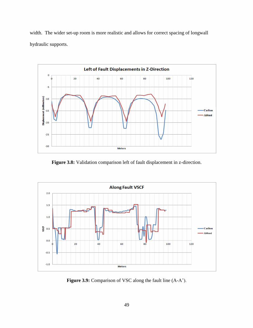
49

width. The wider set-up room is more realistic and allows for correct spacing of longwall

hydraulic supports.

Figure 3.8: Validation comparison left of fault displacement in z-direction.

Figure 3.9: Comparison of VSC along the fault line (A-A’).

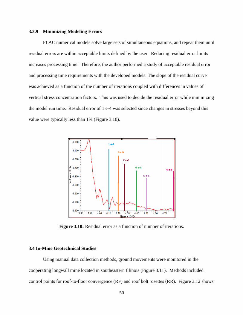
50

3.3.9 Minimizing Modeling Errors

FLAC numerical models solve large sets of simultaneous equations, and repeat them until

residual errors are within acceptable limits defined by the user. Reducing residual error limits

increases processing time. Therefore, the author performed a study of acceptable residual error

and processing time requirements with the developed models. The slope of the residual curve

was achieved as a function of the number of iterations coupled with differences in values of

vertical stress concentration factors. This was used to decide the residual error while minimizing

the model run time. Residual error of 1 e-4 was selected since changes in stresses beyond this

value were typically less than 1% (Figure 3.10).

Figure 3.10: Residual error as a function of number of iterations.

3.4 In-Mine Geotechnical Studies

Using manual data collection methods, ground movements were monitored in the

cooperating longwall mine located in southeastern Illinois (Figure 3.11). Methods included

control points for roof-to-floor convergence (RF) and roof bolt rosettes (RR). Figure 3.12 shows

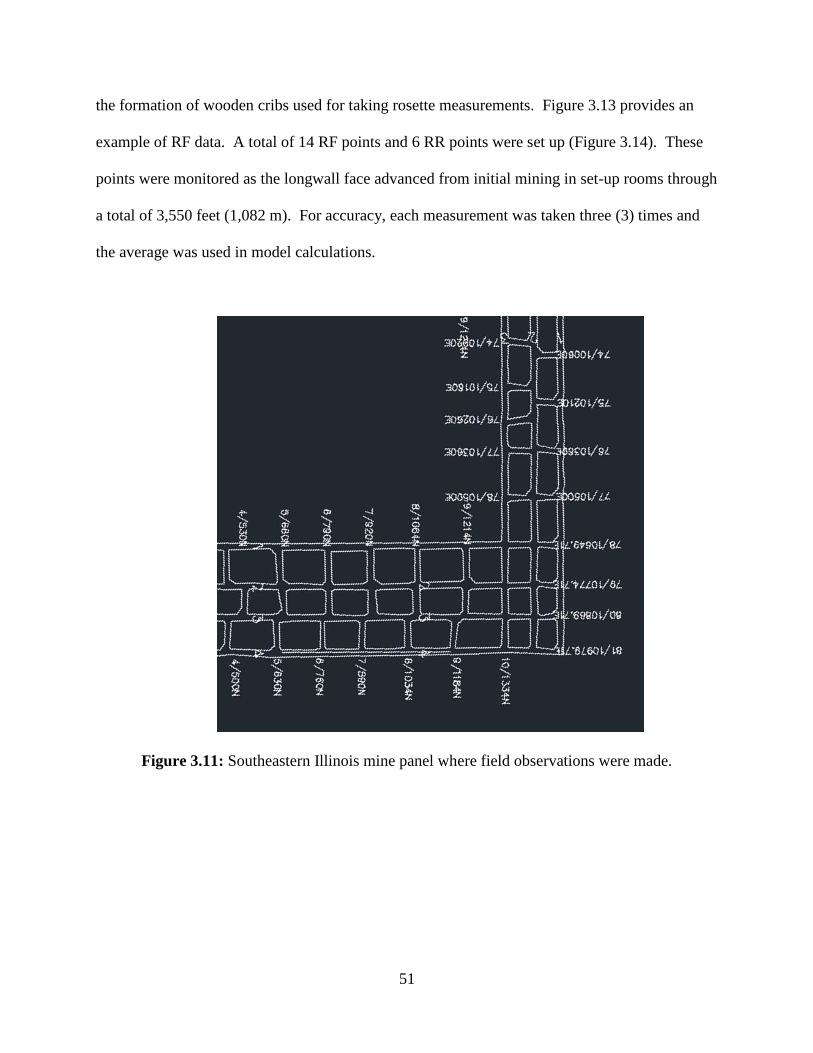
51

the formation of wooden cribs used for taking rosette measurements. Figure 3.13 provides an

example of RF data. A total of 14 RF points and 6 RR points were set up (Figure 3.14). These

points were monitored as the longwall face advanced from initial mining in set-up rooms through

a total of 3,550 feet (1,082 m). For accuracy, each measurement was taken three (3) times and

the average was used in model calculations.

Figure 3.11: Southeastern Illinois mine panel where field observations were made.

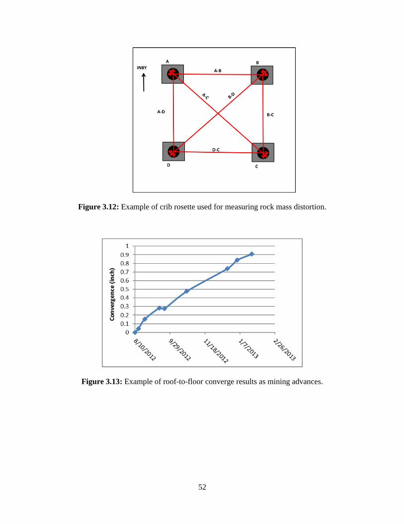
52

Figure 3.12: Example of crib rosette used for measuring rock mass distortion.

Figure 3.13: Example of roof-to-floor converge results as mining advances.

53

Figure 3.14: Location of faults and measurement points.

3.5 Limitations of Model Development and Analysis

Even though attempts were made to simulate the physical problem as accurately as

possible, it is important to identify several important limitations of this effort. These include

modeling limitations, such as model size and number of elements; however, the more significant

limitations have to do with uncertainty in several model inputs. For example, there is uncertainty

in modeling the geometry of the fault plane and adjoining rock mass, whose engineering

properties affected faulting. There is uncertainty in estimating rock mass properties (e.g., GSI

values). There is uncertainty in defining engineering properties adjoining the fault plane and the

variable lithology of immediate roof and floor strata. Despite these limitations, modeling

provides significant insights into load transfer mechanisms between the longwall face,

development gate entries, and the gob.

54

3.6 Analysis of Data from Numerical Modeling

For this study, a total of ten (10) data lines were analyzed from A-A’ to J-J’. Data from

both the roof above the coal seam and the floor below the coal seam was taken from data lines.

Data lines B-B’, C-C’, and D-D’ run along set-up room entries 1 foot (0.3 m) into coal pillars.

Data line E-E’ runs along the panel 1 foot (0.3 m) into the block of coal. Data lines F-F’, G-G’,

H-H’, and I-I’ run along tailgate entries 1 foot (0.3 m) into coal pillars. Their locations were

chosen because stresses redistribute based on geometry and concentrations of stresses occur at

pillar edges. Data line A-A’ runs along the fault. This is a data line for obtaining information

critical to the project’s purpose centering about the fault. All of the previously mentioned data

lines are static throughout all analysis. J-J’ is the only data line whose location changes

depending on the location of the advancing face. This data line was always located 1foot (0.3 m)

into the solid coal block in front of the advancing longwall face. The primary motive for using

this data line was the redistribution of stresses due to caving behind the face. These data lines

can be observed in the plan view of the coal seam level of the model in Figure 3.15.

3.6.1 Displacement Variables

In this study, displacements in both horizontal x and y directions and the vertical z

direction were determined. Roof-to-floor convergence of the coal seam was calculated from

vertical displacements of two (2) points; one (1) point in the roof and one (1) point in the floor

with matching x and y coordinates. Incremental displacements were calculated by subtracting a

point’s displacement at a given face location from the displacement when the face was located at

the previous location. Total displacement of a point was calculated by taking the square root of

the sum of the squares for x-, y-, and z-direction displacements.

55

Figure 3.15: Modeled area with primary data lines used for analysis.

56

CHAPTER 4

ANALYTICAL STUDIES

4.1 Model Analysis

Two models were analyzed with the difference being that Model 1 did not include the

fault zone and Model 2 did include the fault zone. Figure 4.1 shows principal data lines used in

the analysis, as well as distances of longwall face advance within the model. This chapter

presents results describing the effects of the fault on ground control in set-up rooms, the longwall

face area, and longwall development areas on the headgate side.

Figure 4.1: Model depiction with principal data lines (purple), fault zone (green), and face

advance distances (red and yellow).

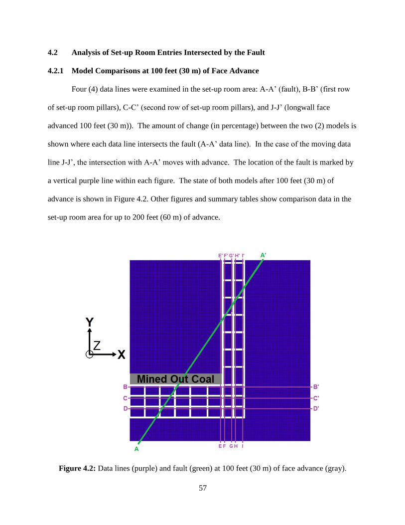
57

4.2 Analysis of Set-up Room Entries Intersected by the Fault

4.2.1 Model Comparisons at 100 feet (30 m) of Face Advance

Four (4) data lines were examined in the set-up room area: A-A’ (fault), B-B’ (first row

of set-up room pillars), C-C’ (second row of set-up room pillars), and J-J’ (longwall face

advanced 100 feet (30 m)). The amount of change (in percentage) between the two (2) models is

shown where each data line intersects the fault (A-A’ data line). In the case of the moving data

line J-J’, the intersection with A-A’ moves with advance. The location of the fault is marked by

a vertical purple line within each figure. The state of both models after 100 feet (30 m) of

advance is shown in Figure 4.2. Other figures and summary tables show comparison data in the

set-up room area for up to 200 feet (60 m) of advance.

Figure 4.2: Data lines (purple) and fault (green) at 100 feet (30 m) of face advance (gray).

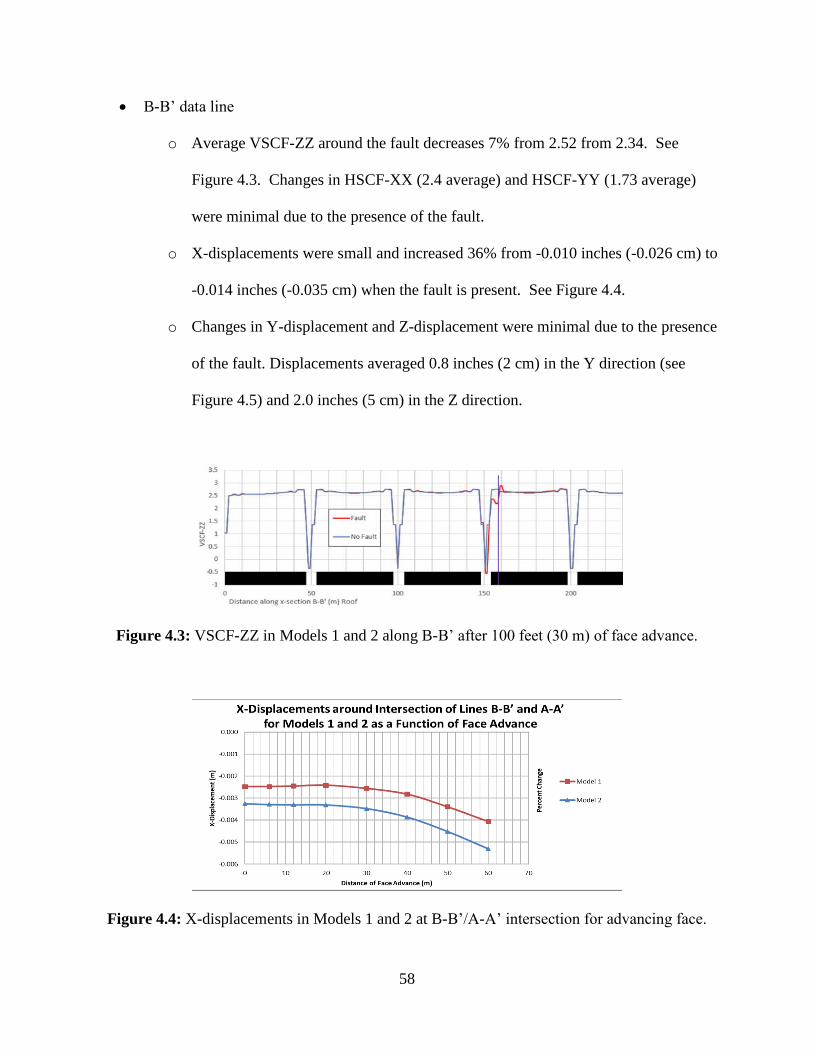
58

• B-B’ data line

o Average VSCF-ZZ around the fault decreases 7% from 2.52 from 2.34. See

Figure 4.3. Changes in HSCF-XX (2.4 average) and HSCF-YY (1.73 average)

were minimal due to the presence of the fault.

o X-displacements were small and increased 36% from -0.010 inches (-0.026 cm) to

-0.014 inches (-0.035 cm) when the fault is present. See Figure 4.4.

o Changes in Y-displacement and Z-displacement were minimal due to the presence

of the fault. Displacements averaged 0.8 inches (2 cm) in the Y direction (see

Figure 4.5) and 2.0 inches (5 cm) in the Z direction.

Figure 4.3: VSCF-ZZ in Models 1 and 2 along B-B’ after 100 feet (30 m) of face advance.

Figure 4.4: X-displacements in Models 1 and 2 at B-B’/A-A’ intersection for advancing face.

59

Figure 4.5: Y-displacements in Models 1 and 2 at B-B’/A-A’ intersection for advancing face.

• C-C’ data line

o Changes in Z-displacement, HSCF-XX, HSCF-YY, and VSCF-ZZ were minimal

due to the fault. Average values were: Z-displacement – 0.4 inches (1 cm),

HSCF-XX – 2.1, HSCF-YY – 1.24, and VSCF-ZZ – 1.28.

o X-displacements were small and only slightly changed due to the presence of the

fault. See Figure 4.6.

o Y-displacements increased 84% from 0.05 inches (0.13 cm) to 0.09 inches

(0.24 cm) due to fault. See Figures 4.7 and 4.8.

Figure 4.6: X-displacements in Models 1 and 2 at C-C’/A-A’ intersection for advancing face.

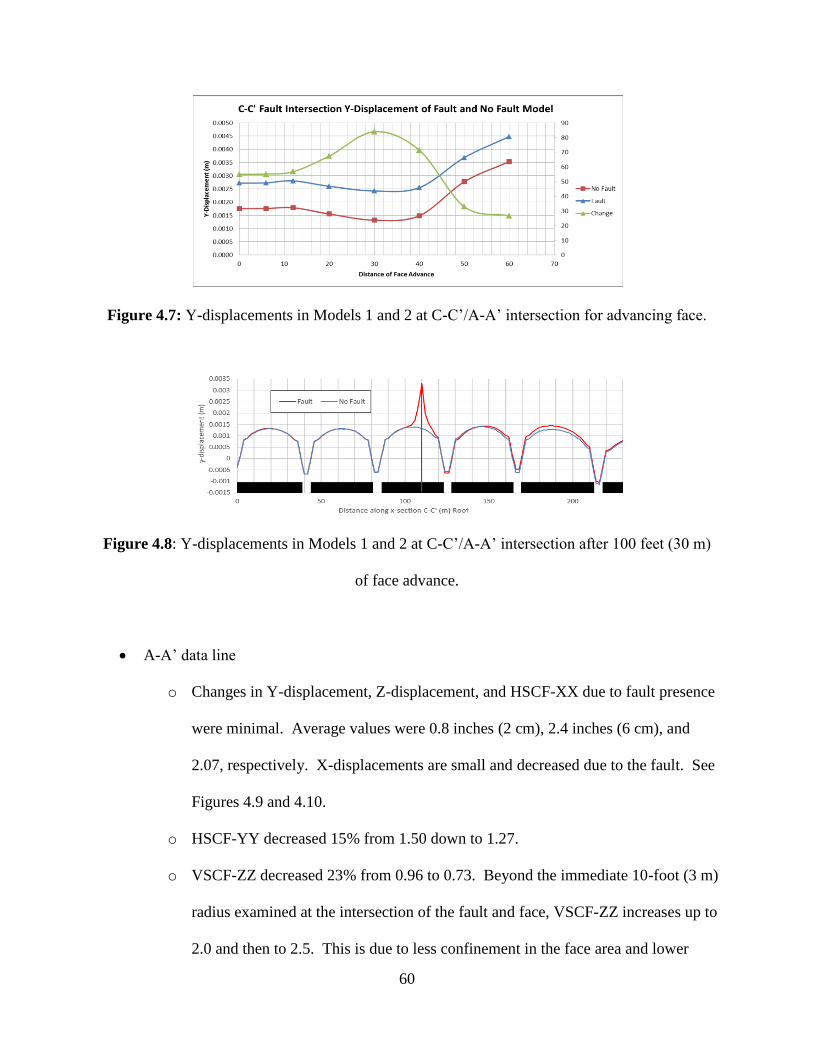
60

Figure 4.7: Y-displacements in Models 1 and 2 at C-C’/A-A’ intersection for advancing face.

Figure 4.8: Y-displacements in Models 1 and 2 at C-C’/A-A’ intersection after 100 feet (30 m)

of face advance.

• A-A’ data line

o Changes in Y-displacement, Z-displacement, and HSCF-XX due to fault presence

were minimal. Average values were 0.8 inches (2 cm), 2.4 inches (6 cm), and

2.07, respectively. X-displacements are small and decreased due to the fault. See

Figures 4.9 and 4.10.

o HSCF-YY decreased 15% from 1.50 down to 1.27.

o VSCF-ZZ decreased 23% from 0.96 to 0.73. Beyond the immediate 10-foot (3 m)

radius examined at the intersection of the fault and face, VSCF-ZZ increases up to

2.0 and then to 2.5. This is due to less confinement in the face area and lower

61

stiffness along the fault. The confined coal solid ahead of the face is picking up

additional load not observed within the radius of examination. See Figure 4.11.

o Averaged VSCF-ZZ values were less than 1.25 for Model 2 and less than 1.13 for

Model 1 for face advances of 0 to 200 feet (60 m). At 66 feet (20 m) of face

advance, Model 2 experienced 15% higher VSCF-ZZ averages; and at 132 feet

(40 m) of face advance, Model 2 experienced 23% higher VSCF-ZZ averages.

Model 1 VSCF-ZZ averages were 23% lower at 98 feet (30 m) and 13% lower at

164 feet (50 m) and 197 feet (60 m).

Figure 4.9: X-displacements in Models 1 and 2 at A-A’/J-J’ intersection for advancing face.

Figure 4.10: Y-displacements in Models 1 and 2 at A-A’/J-J’ intersection for advancing face.

62

Figure 4.11: VSCF-ZZ in Model 2 along A-A’ after 100 feet (30 m) of face advance.

• J-J’ data line

o Changes in Y-displacement, Z-displacement, and HSCF-XX were minimal due to

fault presence. Average values were 0.75 inches (1.9 cm), -2.00 inches (-5 cm),

and 2.52, respectively. X-displacements are small and decrease due to the fault

from 0.059 inches (0.15 cm) for Model 1 to 0.0315 inches (0.08 cm) for Model 2.

See Figures 4.12 through 4.14.

o HSCF-YY decreased about 7% from 1.94 down to 1.8.

o VSCF-ZZ decreased about 15% from 2.75 down to 2.47.

Figure 4.12: X-displacements in Models 1 and 2 along J-J’ after 100 feet (30 m) of face

advance.

63

Figure 4.13: X-displacements in Models 1 and 2 at J-J’/A-A’ intersection for advancing face.

Figure 4.14: Y-displacements in Models 1 and 2 at J-J’/A-A’ intersection for advancing face.

4.2.2 Results Summary of Set-up Room Analysis

• Data pertaining to areas where B-B’, C-C’, and J-J’ intersect the fault and where A-A’

intersects the moving face through 200 feet (60 m) of face advance are presented in

Tables 4.1 through 4.4. Each table shows data from Model 1 in the top section, data from

Model 2 in the middle section, and the percentage change from the base case (Model 1

with no fault) in the bottom section.

64

Table 4.1: Average results for B-B’ data line within ±9.83 feet (3 m) of intersection with fault

for 0 to 200 feet (60 m) of face advance.

Avg (± 3m) B-B' B-B' B-B' B-B' B-B' B-B'

Model 1 x-disp (m) y-disp (m) z-disp (m) HSCF-XX HSCF-YY VSCF-ZZ

0 m -0.0025 -0.0022 -0.0105 2.02 1.06 1.24

6 m -0.0025 -0.0015 -0.0137 2.07 1.08 1.43

12 m -0.0025 0.0020 -0.0241 2.15 1.14 1.80

20 m -0.0024 0.0095 -0.0399 2.29 1.37 2.32

30 m -0.0026 0.0186 -0.0516 2.40 1.73 2.52

40 m -0.0028 0.0265 -0.0576 2.55 2.18 2.82

50 m -0.0034 0.0265 -0.0445 2.50 2.43 2.23

60 m -0.0041 0.0274 -0.0425 2.52 2.56 2.16



0 m -0.0033 -0.0028 -0.0107 1.99 1.08 1.21

6 m -0.0033 -0.0020 -0.0141 2.05 1.13 1.38

12 m -0.0033 0.0015 -0.0246 2.17 1.23 1.71

20 m -0.0033 0.0093 -0.0409 2.35 1.46 2.17

30 m -0.0035 0.0184 -0.0528 2.45 1.67 2.34

40 m -0.0039 0.0265 -0.0590 2.60 1.96 2.61

50 m -0.0045 0.0265 -0.0465 2.47 1.97 2.11

60 m -0.0053 0.0270 -0.0439 2.47 2.02 2.03


Change x-disp (%) y-disp (%) z-disp (%) HSCF-XX (%) HSCF-YY (%) VSCF-ZZ (%)

0 m 31 29 2 -1 2 -2

6 m 33 39 3 -1 4 -3

12 m 35 -26 2 1 8 -5

20 m 37 -3 2 2 6 -6

30 m 36 -1 2 2 -4 -7

40 m 37 0 2 2 -10 -7

50 m 33 0 5 -1 -19 -6

60 m 31 -1 3 -2 -21 -6

65

Table 4.2: Average results for C-C’ data line within ±9.83 feet (3 m) of intersection with fault


Avg (± 3m) C-C' C-C' C-C' C-C' C-C' C-C'


0 m 0.0006 0.0018 -0.0105 2.01 1.11 1.36

6 m 0.0006 0.0018 -0.0109 2.02 1.12 1.37

12 m 0.0005 0.0018 -0.0108 2.02 1.17 1.37

20 m 0.0005 0.0016 -0.0100 2.04 1.25 1.35

30 m 0.0004 0.0013 -0.0087 2.04 1.31 1.31

40 m 0.0001 0.0015 -0.0076 2.04 1.33 1.28

50 m -0.0001 0.0028 -0.0072 2.03 1.27 1.27

60 m -0.0008 0.0035 -0.0069 2.03 1.27 1.26



0 m 0.0007 0.0027 -0.0106 2.09 1.17 1.36

6 m 0.0006 0.0027 -0.0110 2.09 1.17 1.37

12 m 0.0006 0.0028 -0.0109 2.09 1.20 1.36

20 m 0.0006 0.0026 -0.0101 2.10 1.23 1.34

30 m 0.0004 0.0024 -0.0088 2.10 1.24 1.28

40 m 0.0002 0.0025 -0.0077 2.09 1.24 1.26

50 m -0.0001 0.0037 -0.0073 2.08 1.21 1.25

60 m -0.0008 0.0045 -0.0070 2.08 1.20 1.24



0 m 16 55 1 4 5 0

6 m 15 55 1 4 5 -1

12 m 13 57 1 3 3 -1

20 m 10 67 1 3 -1 0

30 m 8 84 1 3 -5 -2

40 m 11 71 1 3 -7 -2

50 m 2 33 1 3 -5 -2

60 m 3 27 1 3 -5 -2

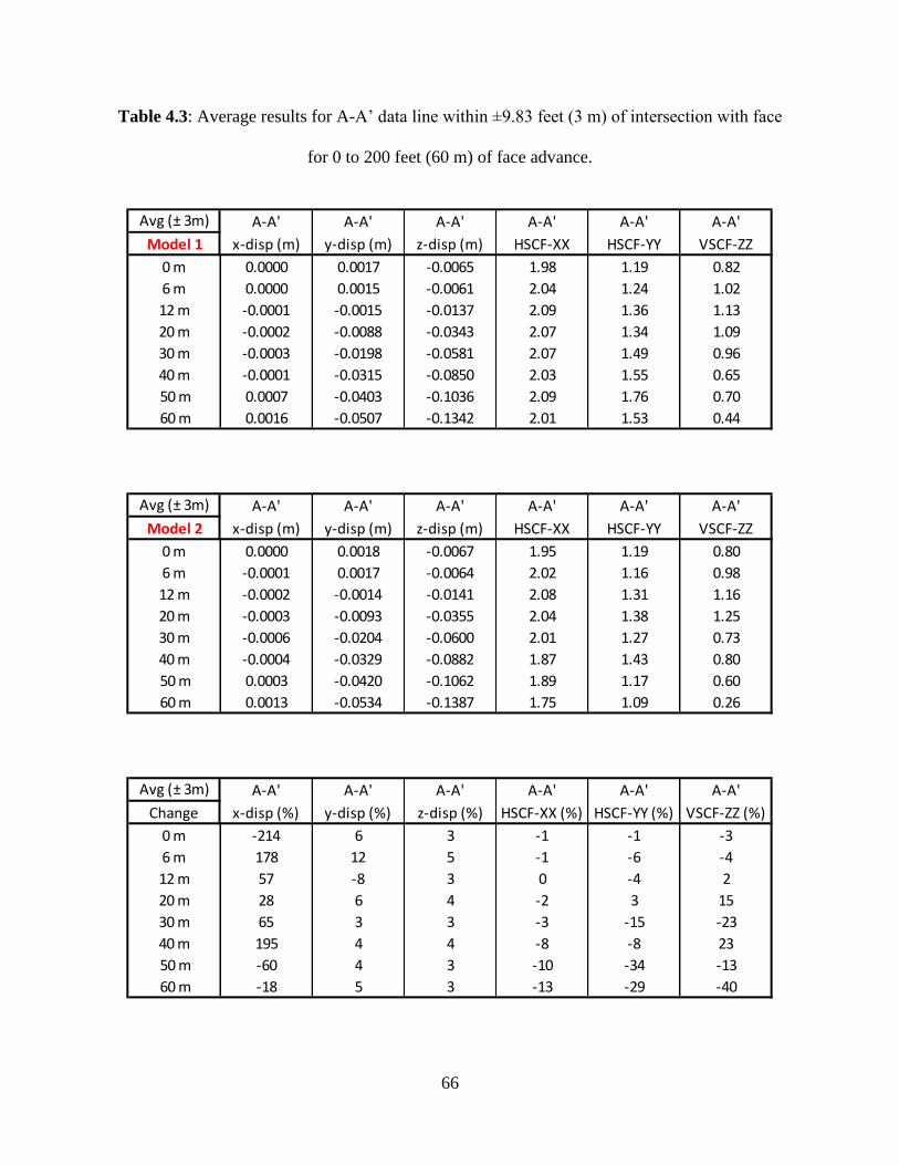
66

Table 4.3: Average results for A-A’ data line within ±9.83 feet (3 m) of intersection with face


Avg (± 3m) A-A' A-A' A-A' A-A' A-A' A-A'


0 m 0.0000 0.0017 -0.0065 1.98 1.19 0.82

6 m 0.0000 0.0015 -0.0061 2.04 1.24 1.02

12 m -0.0001 -0.0015 -0.0137 2.09 1.36 1.13

20 m -0.0002 -0.0088 -0.0343 2.07 1.34 1.09

30 m -0.0003 -0.0198 -0.0581 2.07 1.49 0.96

40 m -0.0001 -0.0315 -0.0850 2.03 1.55 0.65

50 m 0.0007 -0.0403 -0.1036 2.09 1.76 0.70

60 m 0.0016 -0.0507 -0.1342 2.01 1.53 0.44



0 m 0.0000 0.0018 -0.0067 1.95 1.19 0.80

6 m -0.0001 0.0017 -0.0064 2.02 1.16 0.98

12 m -0.0002 -0.0014 -0.0141 2.08 1.31 1.16

20 m -0.0003 -0.0093 -0.0355 2.04 1.38 1.25

30 m -0.0006 -0.0204 -0.0600 2.01 1.27 0.73

40 m -0.0004 -0.0329 -0.0882 1.87 1.43 0.80

50 m 0.0003 -0.0420 -0.1062 1.89 1.17 0.60

60 m 0.0013 -0.0534 -0.1387 1.75 1.09 0.26



0 m -214 6 3 -1 -1 -3

6 m 178 12 5 -1 -6 -4

12 m 57 -8 3 0 -4 2

20 m 28 6 4 -2 3 15

30 m 65 3 3 -3 -15 -23

40 m 195 4 4 -8 -8 23

50 m -60 4 3 -10 -34 -13

60 m -18 5 3 -13 -29 -40

67

Table 4.4: Average results for J-J’ data line within ±9.83 feet (3 m) of intersection with fault for

0 to 200 feet (60 m) of face advance.

Avg (± 3m) J-J' J-J' J-J' J-J' J-J' J-J'


0 m 0.0000 0.0023 -0.0051 2.11 1.20 1.42

6 m 0.0000 0.0017 -0.0065 2.15 1.24 1.57

12 m -0.0001 -0.0015 -0.0156 2.24 1.35 1.94

20 m -0.0002 -0.0084 -0.0344 2.33 1.49 2.24

30 m -0.0004 -0.0185 -0.0498 2.52 1.94 2.75

40 m -0.0001 -0.0281 -0.0626 2.70 2.39 3.18

50 m 0.0007 -0.0363 -0.0767 2.87 2.76 3.64

60 m 0.0014 -0.0436 -0.0859 3.03 3.19 3.95



0 m -0.0001 0.0024 -0.0052 2.11 1.21 1.37

6 m -0.0001 0.0017 -0.0067 2.16 1.24 1.58

12 m -0.0002 -0.0015 -0.0164 2.26 1.35 1.91

20 m -0.0004 -0.0088 -0.0356 2.37 1.51 2.18

30 m -0.0007 -0.0189 -0.0514 2.57 1.80 2.47

40 m -0.0005 -0.0291 -0.0647 2.79 2.15 2.99

50 m 0.0001 -0.0365 -0.0777 2.98 2.40 3.47

60 m 0.0009 -0.0442 -0.0878 3.05 2.51 3.34



0 m -1675 2 2 0 1 -3

6 m 642 0 3 0 1 0

12 m 132 0 5 1 0 -1

20 m 68 5 4 2 1 -3

30 m 90 3 3 2 -7 -10

40 m 297 3 3 3 -10 -6

50 m -89 0 1 4 -13 -5

60 m -39 1 2 1 -21 -15

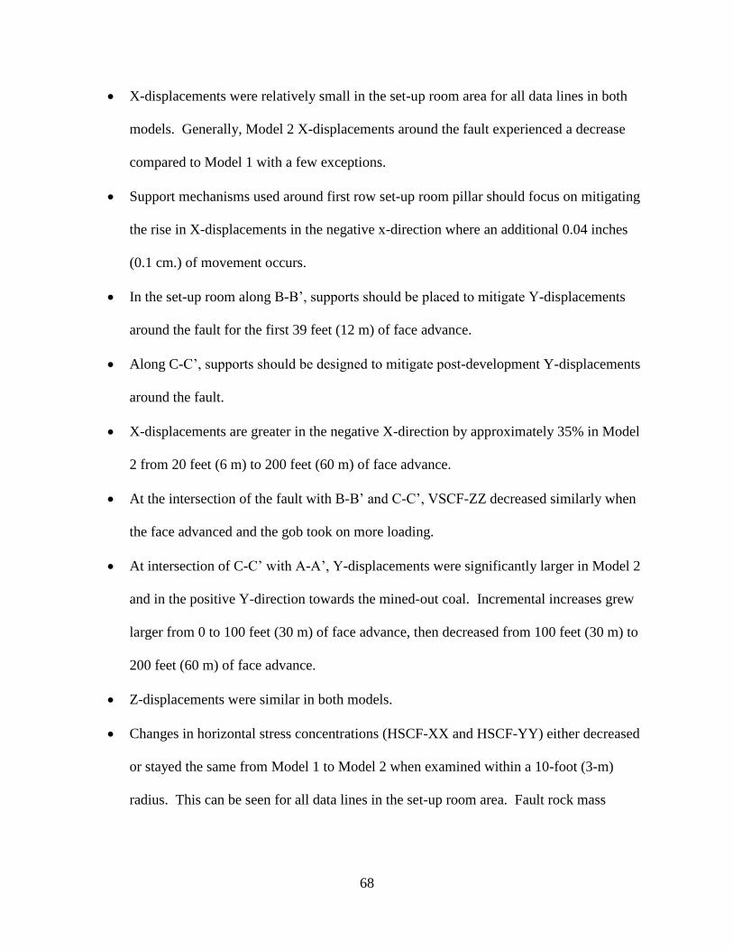
68

• X-displacements were relatively small in the set-up room area for all data lines in both

models. Generally, Model 2 X-displacements around the fault experienced a decrease

compared to Model 1 with a few exceptions.

• Support mechanisms used around first row set-up room pillar should focus on mitigating

the rise in X-displacements in the negative x-direction where an additional 0.04 inches

(0.1 cm.) of movement occurs.

• In the set-up room along B-B’, supports should be placed to mitigate Y-displacements

around the fault for the first 39 feet (12 m) of face advance.

• Along C-C’, supports should be designed to mitigate post-development Y-displacements

around the fault.

• X-displacements are greater in the negative X-direction by approximately 35% in Model

2 from 20 feet (6 m) to 200 feet (60 m) of face advance.

• At the intersection of the fault with B-B’ and C-C’, VSCF-ZZ decreased similarly when

the face advanced and the gob took on more loading.

• At intersection of C-C’ with A-A’, Y-displacements were significantly larger in Model 2

and in the positive Y-direction towards the mined-out coal. Incremental increases grew

larger from 0 to 100 feet (30 m) of face advance, then decreased from 100 feet (30 m) to

200 feet (60 m) of face advance.

• Z-displacements were similar in both models.

• Changes in horizontal stress concentrations (HSCF-XX and HSCF-YY) either decreased

or stayed the same from Model 1 to Model 2 when examined within a 10-foot (3-m)

radius. This can be seen for all data lines in the set-up room area. Fault rock mass

69

material has a lower stiffness than surrounding rock mass and shifts loading around the

geologic anomaly.

• In this specific fault angle and intersection case, horizontal displacements around the

fault are more critical and can show signs of increasing compared to Model 1 whereas

SCF values either stay similar between models or decrease in Model 2.

• The A-A’/J-J’ intersection as well as B-B’ and C-C’ experienced less HSCF-YY in

Model 2 relative to Model 1 with more face advance. For J-J’, after 200 feet (60 m) of

face advance, VSCF-ZZ decreased from Model 1 to Model 2 by 0.6 at the face/fault

intersection.

• SCF increases are very small and in general decrease due to the presence of the fault.

Therefore, enhanced yielding of the rock mass due to changes in SCF values are highly

unlikely.

• On a percentage basis, incremental displacements due to fault can be very large. Thus,

ground control must involve displacement control support measures. Applying high

stiffness control measures can result in the need for high capacity supports. Appropriate

control measures should consist of medium stiffness support systems that will have

increasing resistance and will continue to provide resistance beyond yield. Thus, a strain

hardening model for supports up to the maximum desired value of displacements should

be considered.

• Supports should be installed well ahead of when the following maximum displacements

are likely to occur:

o For the fault/face (A-A’/J-J’) intersection, maximum X-displacement due to the

fault occurs at 98 feet (30 m) of face advance.

70

o For the fault/face (A-A’/J-J’) intersection, maximum Y-displacement due to the

fault occurs at 200 feet (60 m) of face advance.

o For the fault (A-A’)/B-B’ intersection, maximum X-displacement due to the fault

occurs at 200 feet (60 m) of face advance.

o For the fault (A-A’)/B-B’ intersection, maximum Y-displacement due to the fault

occurs between 131 feet (40 m) and 200 feet (60 m) of face advance.

o For the fault (A-A’)/C-C’ intersection, maximum X-displacement due to the fault

occurs at 200 feet (60 m) of face advance.

o For the fault (A-A’)/C-C’ intersection, maximum Y-displacement due to the fault

occurs between 164 feet (50 m) and 200 feet (60 m) of face advance.

4.3 Analysis of Gate Entries Intersected by the Fault

4.3.1 Model Comparisons at 558 feet (170 m) of Face Advance

This face advance distance is considered critical for examination as it is where the fault,

the face, and development gate entries intersect. Most development gate entry mechanized

mining units consist of three (3) entries. They are commonly known as the belt entry next to the

block of coal being mined by the longwall, the intake entry in the center, and the return entry on

the outside. At the fault’s intersection with the three (3) development gate entries, seven (7) data

lines were examined. Shown in Figures 4.1 and 4.2, they are: E-E’ on the inner (next to the

longwall block) side of the belt entry, F-F’ on the outer side of the belt entry, G-G’ on the inner

side of the intake entry, H-H’ on the outer side of the intake entry, I-I’ on the inner side of the

return entry, and the fault and face data lines, A-A’ and J-J’, respectively. Changes between the

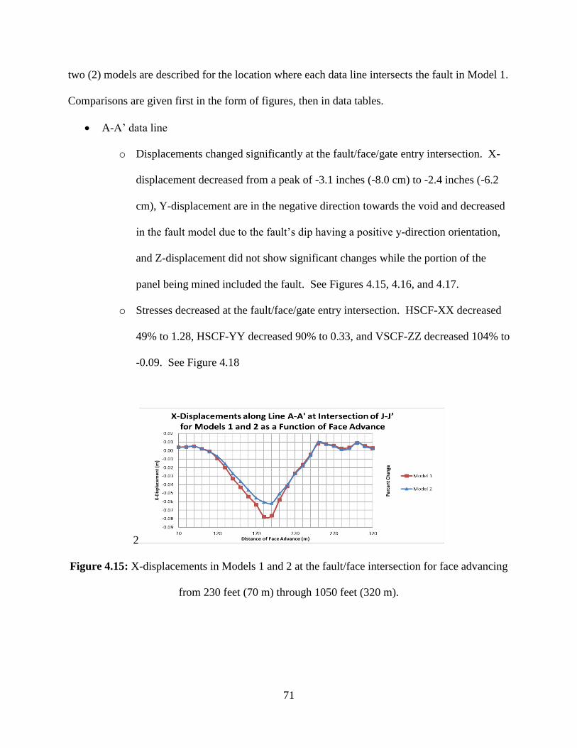
71

two (2) models are described for the location where each data line intersects the fault in Model 1.

Comparisons are given first in the form of figures, then in data tables.


o Displacements changed significantly at the fault/face/gate entry intersection. X-

displacement decreased from a peak of -3.1 inches (-8.0 cm) to -2.4 inches (-6.2

cm), Y-displacement are in the negative direction towards the void and decreased

in the fault model due to the fault’s dip having a positive y-direction orientation,

and Z-displacement did not show significant changes while the portion of the

panel being mined included the fault. See Figures 4.15, 4.16, and 4.17.

o Stresses decreased at the fault/face/gate entry intersection. HSCF-XX decreased

49% to 1.28, HSCF-YY decreased 90% to 0.33, and VSCF-ZZ decreased 104% to

-0.09. See Figure 4.18

2

Figure 4.15: X-displacements in Models 1 and 2 at the fault/face intersection for face advancing

from 230 feet (70 m) through 1050 feet (320 m).

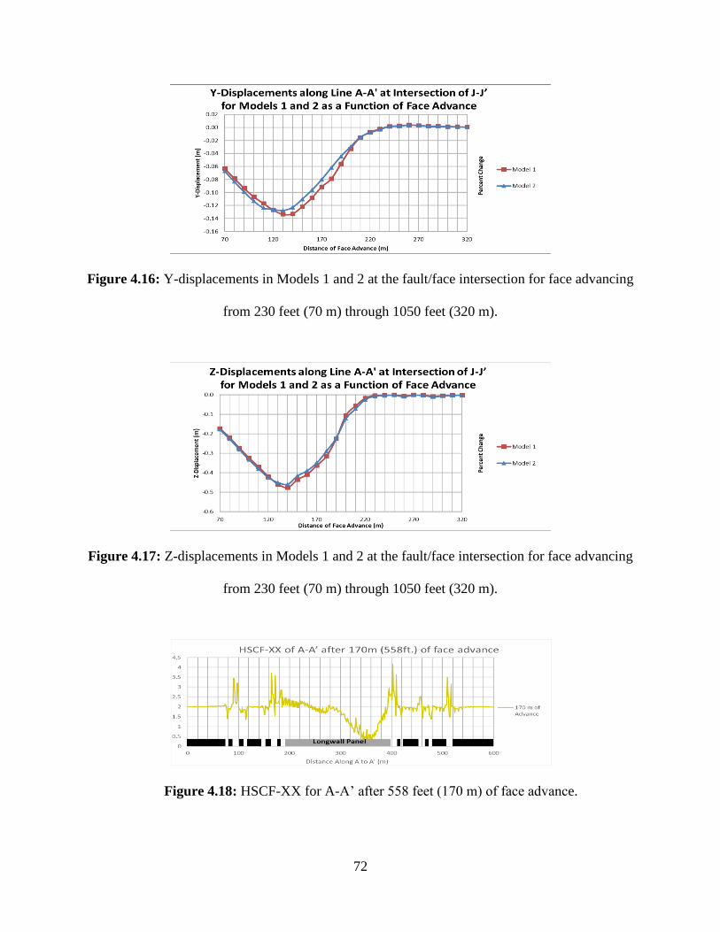
72

Figure 4.16: Y-displacements in Models 1 and 2 at the fault/face intersection for face advancing


Figure 4.17: Z-displacements in Models 1 and 2 at the fault/face intersection for face advancing


Figure 4.18: HSCF-XX for A-A’ after 558 feet (170 m) of face advance.

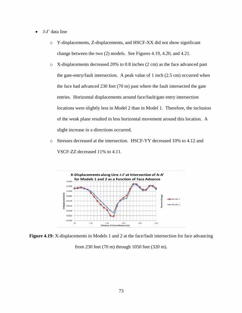
73


o Y-displacements, Z-displacements, and HSCF-XX did not show significant

change between the two (2) models. See Figures 4.19, 4.20, and 4.21.

o X-displacements decreased 20% to 0.8 inches (2 cm) as the face advanced past

the gate-entry/fault intersection. A peak value of 1 inch (2.5 cm) occurred when

the face had advanced 230 feet (70 m) past where the fault intersected the gate

entries. Horizontal displacements around face/fault/gate entry intersection

locations were slightly less in Model 2 than in Model 1. Therefore, the inclusion

of the weak plane resulted in less horizontal movement around this location. A

slight increase in z-directions occurred.

o Stresses decreased at the intersection. HSCF-YY decreased 10% to 4.12 and

VSCF-ZZ decreased 11% to 4.11.

Figure 4.19: X-displacements in Models 1 and 2 at the face/fault intersection for face advancing


74

Figure 4.20: Y-displacements in Models 1 and 2 at the face/fault intersection for face advancing


Figure 4.21: Z-displacements in Models 1 and 2 at the face/fault intersection for face advancing


Figure 4.22: HSCF-XX for J-J’ after 558 feet (170 m) of face advance.

75

Figure 4.23: Model 2 vectors showing horizontal displacement around face/fault intersection for

558 feet (170 m) of face advance.

Figure 4.24: Model 2 vectors showing horizontal displacement around gate-entry intersection

with fault for 558 feet (170 m) of face advance.

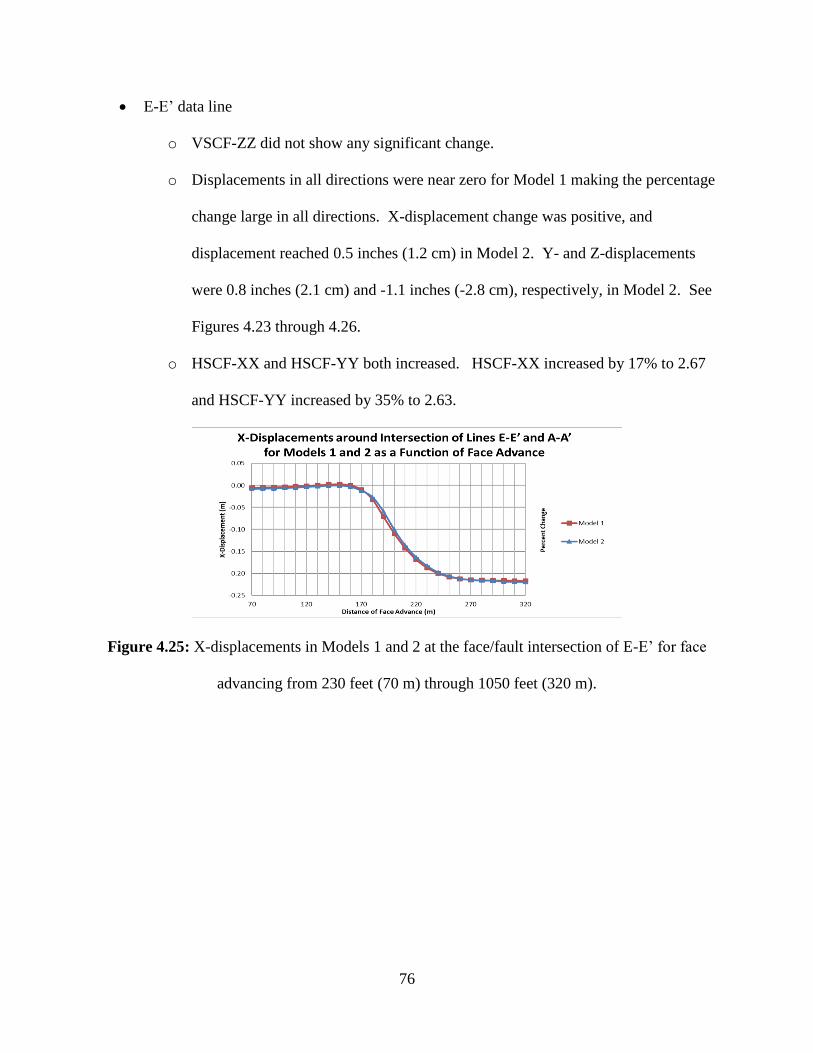
76

• E-E’ data line

o VSCF-ZZ did not show any significant change.

o Displacements in all directions were near zero for Model 1 making the percentage

change large in all directions. X-displacement change was positive, and

displacement reached 0.5 inches (1.2 cm) in Model 2. Y- and Z-displacements

were 0.8 inches (2.1 cm) and -1.1 inches (-2.8 cm), respectively, in Model 2. See

Figures 4.23 through 4.26.

o HSCF-XX and HSCF-YY both increased. HSCF-XX increased by 17% to 2.67

and HSCF-YY increased by 35% to 2.63.

Figure 4.25: X-displacements in Models 1 and 2 at the face/fault intersection of E-E’ for face

advancing from 230 feet (70 m) through 1050 feet (320 m).

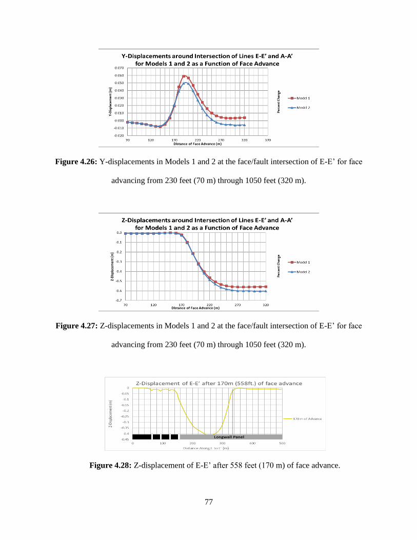
77

Figure 4.26: Y-displacements in Models 1 and 2 at the face/fault intersection of E-E’ for face


Figure 4.27: Z-displacements in Models 1 and 2 at the face/fault intersection of E-E’ for face


Figure 4.28: Z-displacement of E-E’ after 558 feet (170 m) of face advance.

78

• F-F’ data line

o As shown in Figures 4.27, 4.28, and 4.29, X- and Y-displacements increased 16%

and 86% to 0.43 inches (1.1 cm) and 168% to 0.2 inches (0.5 cm), respectively,

while Z-displacements increased 56% to -0.49 inches (-1.24 cm).

o All horizontal SCFs remained similar between models. VSCF-ZZ increased 13%

to 1.45.

Figure 4.29: X-displacements in Models 1 and 2 at the face/fault intersection of F-F’ for face


Figure 4.30: Y-displacements in Models 1 and 2 at the face/fault intersection of F-F’ for face


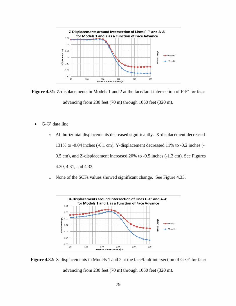
79

Figure 4.31: Z-displacements in Models 1 and 2 at the face/fault intersection of F-F’ for face


• G-G’ data line

o All horizontal displacements decreased significantly. X-displacement decreased

131% to -0.04 inches (-0.1 cm), Y-displacement decreased 11% to -0.2 inches (-

0.5 cm), and Z-displacement increased 20% to -0.5 inches (-1.2 cm). See Figures

4.30, 4.31, and 4.32

o None of the SCFs values showed significant change. See Figure 4.33.

Figure 4.32: X-displacements in Models 1 and 2 at the face/fault intersection of G-G’ for face


80

Figure 4.33 Y-displacements in Models 1 and 2 at the face/fault intersection of G-G’ for face


Figure 4.34: Z-displacements in Models 1 and 2 at the face/fault intersection of G-G’ for face


Figure 4.35: VSCF-ZZ of G-G’ after 558 feet (170 m) of face advance.

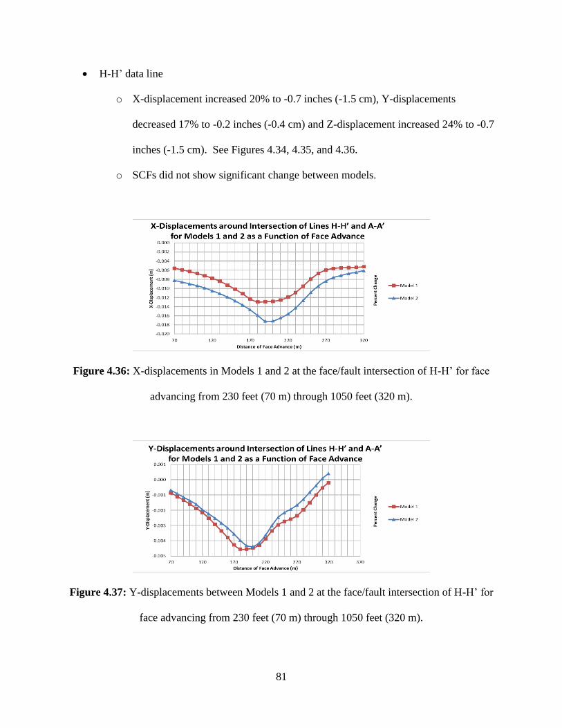
81

• H-H’ data line

o X-displacement increased 20% to -0.7 inches (-1.5 cm), Y-displacements

decreased 17% to -0.2 inches (-0.4 cm) and Z-displacement increased 24% to -0.7

inches (-1.5 cm). See Figures 4.34, 4.35, and 4.36.

o SCFs did not show significant change between models.

Figure 4.36: X-displacements in Models 1 and 2 at the face/fault intersection of H-H’ for face


Figure 4.37: Y-displacements between Models 1 and 2 at the face/fault intersection of H-H’ for

face advancing from 230 feet (70 m) through 1050 feet (320 m).

82

Figure 4.38: Z-displacements in Models 1 and 2 at the face/fault intersection of H-H’ for face


• I-I’ data line

o X-displacement decreased 204% to -0.01 inches (-0.02 cm), Y-displacements

decreased 14% to -0.1 inches (-0.2 cm), and Z-displacement increased 24% to -

0.4 inches (-1.1 cm). See Figures 4.37, 4.38, and 4.39.

o SCFs did not show significant change between models. See Figure 4.38.

Figure 4.39: X-displacements in Models 1 and 2 at the face/fault intersection of I-I’ for face


83

Figure 4.40: Y-displacements in Models 1 and 2 at the face/fault intersection of I-I’ for face


Figure 4.41: Z-displacements in Models 1 and 2 at the face/fault intersection of I-I’ for face


84

Table 4.5: Average results for A-A’ data line within ±9.83 feet (3 m) of intersection with the

lateral face location for Model 1 advancing from 230 feet (70 m) through 1050 feet (320 m).



70 m 0.0039 -0.0630 -0.1730 1.88 1.13 0.11

80 m 0.0043 -0.0782 -0.2203 1.84 1.17 0.13

90 m 0.0051 -0.0933 -0.2734 1.71 1.05 0.15

100 m 0.0021 -0.1065 -0.3243 1.57 1.05 0.09

110 m -0.0011 -0.1168 -0.3709 1.35 0.94 0.04

120 m -0.0094 -0.1267 -0.4197 1.17 0.91 0.04

130 m -0.0198 -0.1335 -0.4595 0.96 0.78 0.04

140 m -0.0330 -0.1328 -0.4765 0.87 0.69 0.04

150 m -0.0432 -0.1218 -0.4359 0.89 0.77 0.05

160 m -0.0541 -0.1084 -0.4094 0.94 0.58 0.03

170 m -0.0635 -0.0914 -0.3631 1.25 0.54 0.02

180 m -0.0775 -0.0790 -0.3151 2.04 0.72 0.01

190 m -0.0766 -0.0560 -0.2258 3.14 0.98 0.01

200 m -0.0579 -0.0326 -0.1071 6.21 1.92 2.37

210 m -0.0419 -0.0153 -0.0576 4.68 2.03 1.19

220 m -0.0265 -0.0072 -0.0177 4.00 1.37 1.66

220 m -0.0165 -0.0022 -0.0036 3.28 1.32 1.09

240 m -0.0046 0.0018 -0.0016 3.68 1.37 0.72

250 m 0.0080 0.0025 -0.0006 2.97 1.20 0.90

260 m 0.0074 0.0038 -0.0071 2.06 1.28 0.47

270 m 0.0058 0.0032 -0.0010 1.87 0.95 1.08

280 m 0.0026 0.0022 -0.0024 1.70 1.02 1.06

290 m 0.0037 0.0021 -0.0089 2.57 1.17 0.84

300 m 0.0090 0.0015 -0.0053 2.36 1.15 1.00

310 m 0.0055 0.0011 -0.0029 1.68 1.04 1.10

320 m 0.0032 0.0008 -0.0015 1.85 1.06 1.06

85

Table 4.6: Average results for A-A’ data line within ±9.83 feet (3 m) of intersection with the

lateral face location for Model 2 advancing from 230 feet (70 m) through 1050 feet (320 m).



70 m 0.0038 -0.0670 -0.1789 1.56 0.68 0.10

80 m 0.0041 -0.0834 -0.2277 1.54 0.75 0.12

90 m 0.0051 -0.0989 -0.2809 1.49 0.67 0.07

100 m 0.0019 -0.1131 -0.3339 1.48 0.86 -0.17

110 m -0.0015 -0.1237 -0.3813 1.31 0.66 -0.30

120 m -0.0068 -0.1261 -0.4257 1.20 0.61 -0.30

130 m -0.0155 -0.1277 -0.4517 1.02 0.42 -0.07

140 m -0.0269 -0.1230 -0.4601 0.93 0.28 -0.06

150 m -0.0361 -0.1104 -0.4174 0.95 0.29 -0.10

160 m -0.0463 -0.0964 -0.3905 1.09 0.32 -0.12

170 m -0.0556 -0.0803 -0.3502 1.28 0.33 -0.09

180 m -0.0604 -0.0620 -0.2897 1.68 0.38 -0.18

190 m -0.0619 -0.0444 -0.2225 2.17 0.57 -0.10

200 m -0.0508 -0.0294 -0.1235 4.24 1.42 1.99

210 m -0.0403 -0.0146 -0.0725 3.23 1.43 0.65

220 m -0.0272 -0.0080 -0.0254 3.48 1.38 1.84

220 m -0.0180 -0.0030 -0.0075 2.81 1.27 1.17

240 m -0.0056 0.0016 -0.0045 2.87 1.27 0.79

250 m 0.0100 0.0021 -0.0022 2.10 1.00 0.81

260 m 0.0071 0.0038 -0.0103 1.75 0.98 0.50

270 m 0.0051 0.0030 -0.0022 1.98 1.04 1.05

280 m 0.0013 0.0018 -0.0038 1.88 1.05 1.04

290 m 0.0025 0.0018 -0.0115 2.32 1.14 0.93

300 m 0.0095 0.0013 -0.0065 2.05 1.05 0.82

310 m 0.0047 0.0009 -0.0037 1.88 1.07 1.06

320 m 0.0022 0.0006 -0.0019 1.94 1.09 1.06

86

Table 4.7: Percent change between Models 1 and 2 for A-A’ data line within ±9.83 feet (3 m) of

Model 2 fault intersection for face advancing from 230 feet (70 m) through 1050 feet (320 m).



70 m -1 6 3 -17 -40 -10

80 m -5 7 3 -17 -36 -9

90 m 0 6 3 -13 -36 -55

100 m -11 6 3 -6 -18 -287

110 m 33 6 3 -3 -30 -812

120 m -28 0 1 3 -33 -862

130 m -22 -4 -2 6 -47 -267

140 m -18 -7 -3 7 -59 -271

150 m -16 -9 -4 6 -62 -323

160 m -14 -11 -5 15 -45 -497

170 m -12 -12 -4 3 -39 -586

180 m -22 -22 -8 -18 -47 -1470

190 m -19 -21 -1 -31 -42 -747

200 m -12 -10 15 -32 -26 -16

210 m -4 -4 26 -31 -30 -45

220 m 3 12 44 -13 1 11

230 m 9 36 111 -14 -4 7

240 m 23 -14 177 -22 -7 10

250 m 25 -18 280 -29 -16 -10

260 m -4 0 45 -15 -23 5

270 m -13 -8 120 6 9 -2

280 m -52 -17 57 11 3 -2

290 m -32 -12 29 -10 -3 12

300 m 6 -14 24 -13 -9 -18

310 m -14 -17 27 12 3 -3

320 m -30 -22 28 5 2 0

87

Table 4.8: Average results for Model 1 J-J’ data line within ±9.83 feet (3 m) of intersection with

Model 2 fault for face advancing from 230 feet (70 m) through 1050 feet (320 m).



70 m 0.0031 -0.0520 -0.0971 3.20 3.64 4.33

80 m 0.0035 -0.0619 -0.1090 3.36 4.19 4.74

90 m 0.0040 -0.0717 -0.1219 3.50 4.72 5.18

100 m 0.0029 -0.0798 -0.1317 3.62 5.18 5.53

110 m 0.0016 -0.0855 -0.1385 3.68 5.53 5.77

120 m -0.0017 -0.0909 -0.1451 3.73 5.90 6.03

130 m -0.0056 -0.0935 -0.1475 3.73 6.12 6.16

140 m -0.0100 -0.0908 -0.1426 3.67 6.09 6.05

150 m -0.0136 -0.0831 -0.1313 3.54 5.76 5.71

160 m -0.0167 -0.0727 -0.1162 3.38 5.29 5.25

170 m -0.0192 -0.0601 -0.0976 3.20 4.70 4.66

180 m -0.0248 -0.0512 -0.0815 3.08 4.22 4.12

190 m -0.0254 -0.0389 -0.0694 3.01 3.33 3.09

200 m -0.0152 -0.0230 -0.0403 3.76 2.55 0.97

210 m -0.0094 -0.0123 -0.0148 2.72 1.94 1.55

220 m -0.0066 -0.0053 -0.0046 2.53 1.55 1.16

230 m -0.0043 -0.0016 -0.0025 2.35 1.20 1.07

240 m 0.0021 0.0023 -0.0141 2.49 1.49 0.53

250 m 0.0073 0.0030 -0.0058 2.85 1.15 0.60

260 m 0.0071 0.0026 -0.0021 1.82 1.07 1.04

270 m 0.0044 0.0024 -0.0027 1.80 1.04 1.09

280 m 0.0018 0.0009 -0.0060 1.78 0.98 1.21

290 m 0.0018 0.0027 -0.0122 2.05 1.05 1.24

300 m 0.0055 0.0012 -0.0100 2.58 1.11 0.63

310 m 0.0056 0.0008 -0.0041 1.78 1.07 1.12

320 m 0.0029 0.0006 -0.0024 1.82 1.06 1.08

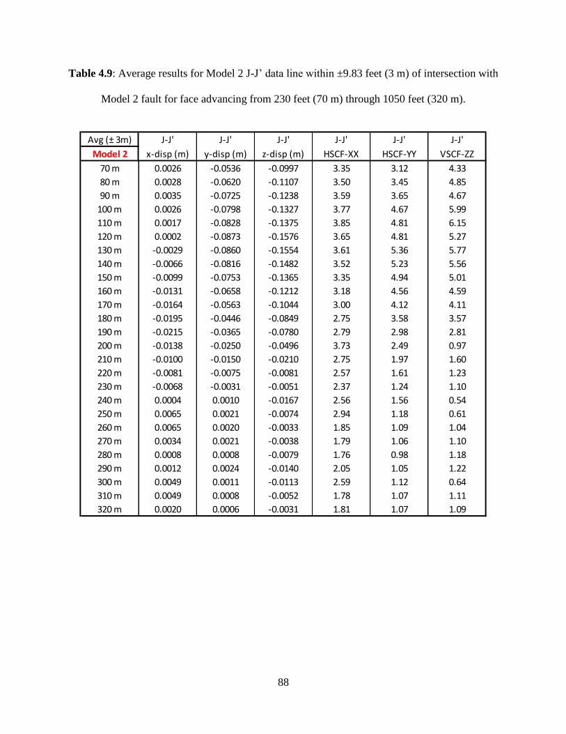
88

Table 4.9: Average results for Model 2 J-J’ data line within ±9.83 feet (3 m) of intersection with

Model 2 fault for face advancing from 230 feet (70 m) through 1050 feet (320 m).



70 m 0.0026 -0.0536 -0.0997 3.35 3.12 4.33

80 m 0.0028 -0.0620 -0.1107 3.50 3.45 4.85

90 m 0.0035 -0.0725 -0.1238 3.59 3.65 4.67

100 m 0.0026 -0.0798 -0.1327 3.77 4.67 5.99

110 m 0.0017 -0.0828 -0.1375 3.85 4.81 6.15

120 m 0.0002 -0.0873 -0.1576 3.65 4.81 5.27

130 m -0.0029 -0.0860 -0.1554 3.61 5.36 5.77

140 m -0.0066 -0.0816 -0.1482 3.52 5.23 5.56

150 m -0.0099 -0.0753 -0.1365 3.35 4.94 5.01

160 m -0.0131 -0.0658 -0.1212 3.18 4.56 4.59

170 m -0.0164 -0.0563 -0.1044 3.00 4.12 4.11

180 m -0.0195 -0.0446 -0.0849 2.75 3.58 3.57

190 m -0.0215 -0.0365 -0.0780 2.79 2.98 2.81

200 m -0.0138 -0.0250 -0.0496 3.73 2.49 0.97

210 m -0.0100 -0.0150 -0.0210 2.75 1.97 1.60

220 m -0.0081 -0.0075 -0.0081 2.57 1.61 1.23

230 m -0.0068 -0.0031 -0.0051 2.37 1.24 1.10

240 m 0.0004 0.0010 -0.0167 2.56 1.56 0.54

250 m 0.0065 0.0021 -0.0074 2.94 1.18 0.61

260 m 0.0065 0.0020 -0.0033 1.85 1.09 1.04

270 m 0.0034 0.0021 -0.0038 1.79 1.06 1.10

280 m 0.0008 0.0008 -0.0079 1.76 0.98 1.18

290 m 0.0012 0.0024 -0.0140 2.05 1.05 1.22

300 m 0.0049 0.0011 -0.0113 2.59 1.12 0.64

310 m 0.0049 0.0008 -0.0052 1.78 1.07 1.11

320 m 0.0020 0.0006 -0.0031 1.81 1.07 1.09

89

Table 4.10: Percent change in J-J’ data line within ±9.83 feet (3 m) of Model 2 fault intersection

for face advancing from 230 feet (70 m) through 1050 feet (320 m).



70 m -17 3 3 5 -14 0

80 m -20 0 2 4 -18 2

90 m -12 1 2 3 -23 -10

100 m -10 0 1 4 -10 8

110 m 1 -3 -1 5 -13 7

120 m -110 -4 9 -2 -18 -13

130 m -48 -8 5 -3 -13 -6

140 m -34 -10 4 -4 -14 -8

150 m -27 -9 4 -5 -14 -12

160 m -22 -9 4 -6 -14 -13

170 m -15 -6 7 -6 -12 -12

180 m -21 -13 4 -11 -15 -13

190 m -15 -6 12 -7 -11 -9

200 m -9 8 23 -1 -3 0

210 m 6 22 42 1 2 3

220 m 23 42 75 2 4 6

230 m 59 92 104 1 3 2

240 m -82 -55 19 2 4 2

250 m -11 -29 28 3 3 2

260 m -9 -23 58 2 2 0

270 m -22 -15 41 -1 2 1

280 m -58 -14 31 -1 0 -3

290 m -36 -8 14 0 0 -2

300 m -12 -11 12 0 1 0

310 m -12 -3 25 0 0 -1

320 m -29 4 27 -1 0 1

90

Table 4.11: Average results for Model 1 E-E’ data line within ±9.83 feet (3 m) of intersection

with Model 2 fault for face advancing from 230 feet (70 m) through 1050 feet (320 m).

Avg (± 3m) E-E' E-E' E-E' E-E' E-E' E-E'


70 m -0.0053 -0.0022 -0.0079 2.08 1.15 1.27

80 m -0.0047 -0.0027 -0.0079 2.08 1.14 1.27

90 m -0.0040 -0.0033 -0.0079 2.08 1.14 1.27

100 m -0.0032 -0.0041 -0.0078 2.08 1.12 1.27

110 m -0.0023 -0.0050 -0.0075 2.08 1.11 1.26

120 m -0.0010 -0.0063 -0.0067 2.08 1.10 1.25

130 m 0.0006 -0.0075 -0.0051 2.08 1.13 1.21

140 m 0.0021 -0.0079 -0.0026 2.11 1.25 1.15

150 m 0.0027 -0.0051 -0.0005 2.18 1.56 1.11

160 m 0.0002 0.0035 -0.0034 2.35 2.13 1.23

170 m -0.0092 0.0194 -0.0219 2.60 2.58 1.98

180 m -0.0315 0.0449 -0.0983 2.85 2.38 0.26

190 m -0.0705 0.0589 -0.2165 3.07 1.13 -0.02

200 m -0.1092 0.0567 -0.3189 3.47 0.57 -0.03

210 m -0.1425 0.0468 -0.4032 3.89 0.42 -0.03

220 m -0.1686 0.0349 -0.4656 4.28 0.53 -0.04

230 m -0.1872 0.0243 -0.5077 4.34 0.91 -0.04

240 m -0.1997 0.0159 -0.5340 4.55 1.11 -0.04

250 m -0.2076 0.0101 -0.5494 4.69 1.27 -0.04

260 m -0.2122 0.0065 -0.5573 4.76 1.39 -0.05

270 m -0.2145 0.0045 -0.5608 4.80 1.46 -0.05

280 m -0.2156 0.0035 -0.5615 4.81 1.51 -0.05

290 m -0.2161 0.0033 -0.5607 4.82 1.54 -0.05

300 m -0.2163 0.0035 -0.5594 4.82 1.55 -0.05

310 m -0.2165 0.0038 -0.5583 4.81 1.54 -0.05

320 m -0.2169 0.0040 -0.5574 4.81 1.53 -0.05

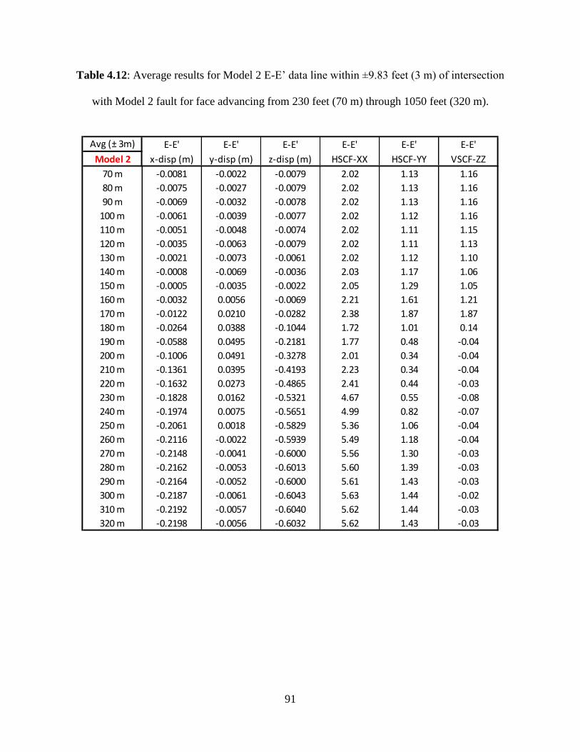
91

Table 4.12: Average results for Model 2 E-E’ data line within ±9.83 feet (3 m) of intersection




70 m -0.0081 -0.0022 -0.0079 2.02 1.13 1.16

80 m -0.0075 -0.0027 -0.0079 2.02 1.13 1.16

90 m -0.0069 -0.0032 -0.0078 2.02 1.13 1.16

100 m -0.0061 -0.0039 -0.0077 2.02 1.12 1.16

110 m -0.0051 -0.0048 -0.0074 2.02 1.11 1.15

120 m -0.0035 -0.0063 -0.0079 2.02 1.11 1.13

130 m -0.0021 -0.0073 -0.0061 2.02 1.12 1.10

140 m -0.0008 -0.0069 -0.0036 2.03 1.17 1.06

150 m -0.0005 -0.0035 -0.0022 2.05 1.29 1.05

160 m -0.0032 0.0056 -0.0069 2.21 1.61 1.21

170 m -0.0122 0.0210 -0.0282 2.38 1.87 1.87

180 m -0.0264 0.0388 -0.1044 1.72 1.01 0.14

190 m -0.0588 0.0495 -0.2181 1.77 0.48 -0.04

200 m -0.1006 0.0491 -0.3278 2.01 0.34 -0.04

210 m -0.1361 0.0395 -0.4193 2.23 0.34 -0.04

220 m -0.1632 0.0273 -0.4865 2.41 0.44 -0.03

230 m -0.1828 0.0162 -0.5321 4.67 0.55 -0.08

240 m -0.1974 0.0075 -0.5651 4.99 0.82 -0.07

250 m -0.2061 0.0018 -0.5829 5.36 1.06 -0.04

260 m -0.2116 -0.0022 -0.5939 5.49 1.18 -0.04

270 m -0.2148 -0.0041 -0.6000 5.56 1.30 -0.03

280 m -0.2162 -0.0053 -0.6013 5.60 1.39 -0.03

290 m -0.2164 -0.0052 -0.6000 5.61 1.43 -0.03

300 m -0.2187 -0.0061 -0.6043 5.63 1.44 -0.02

310 m -0.2192 -0.0057 -0.6040 5.62 1.44 -0.03

320 m -0.2198 -0.0056 -0.6032 5.62 1.43 -0.03

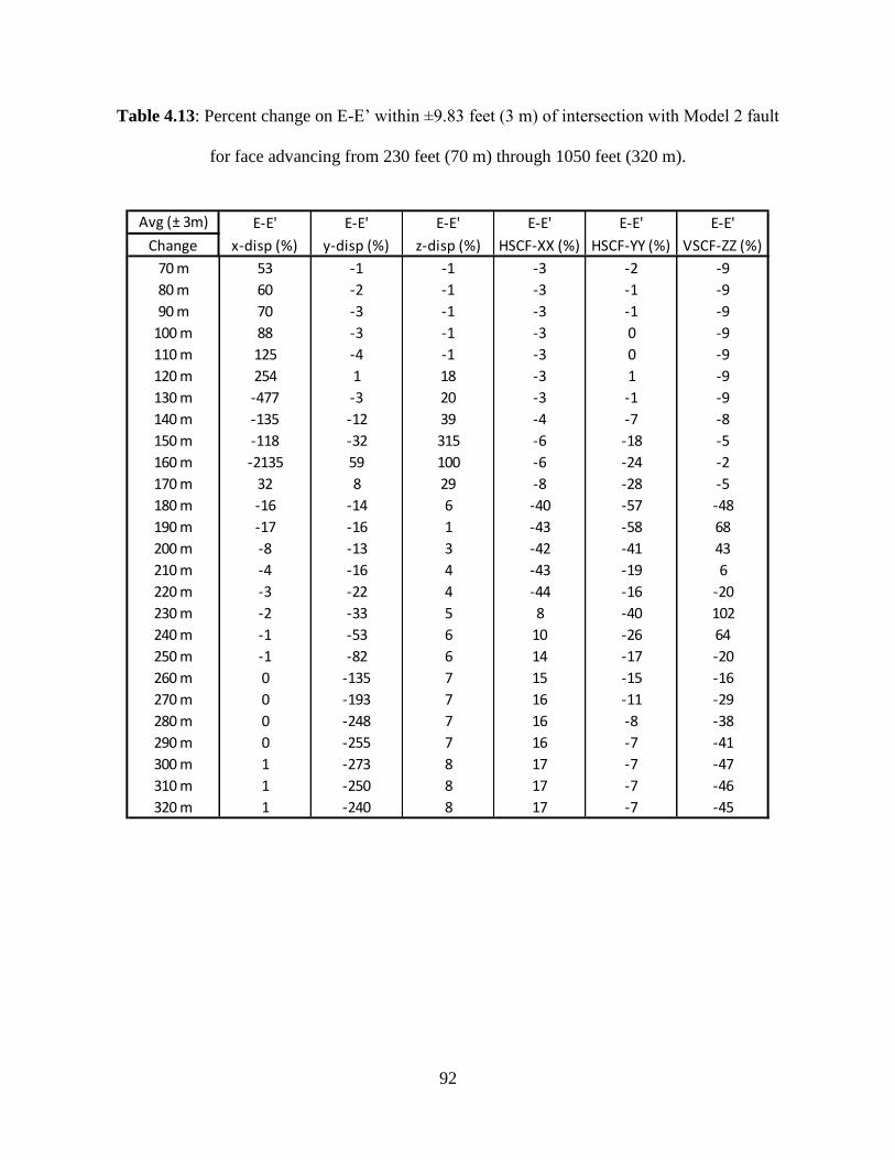
92

Table 4.13: Percent change on E-E’ within ±9.83 feet (3 m) of intersection with Model 2 fault




70 m 53 -1 -1 -3 -2 -9

80 m 60 -2 -1 -3 -1 -9

90 m 70 -3 -1 -3 -1 -9

100 m 88 -3 -1 -3 0 -9

110 m 125 -4 -1 -3 0 -9

120 m 254 1 18 -3 1 -9

130 m -477 -3 20 -3 -1 -9

140 m -135 -12 39 -4 -7 -8

150 m -118 -32 315 -6 -18 -5

160 m -2135 59 100 -6 -24 -2

170 m 32 8 29 -8 -28 -5

180 m -16 -14 6 -40 -57 -48

190 m -17 -16 1 -43 -58 68

200 m -8 -13 3 -42 -41 43

210 m -4 -16 4 -43 -19 6

220 m -3 -22 4 -44 -16 -20

230 m -2 -33 5 8 -40 102

240 m -1 -53 6 10 -26 64

250 m -1 -82 6 14 -17 -20

260 m 0 -135 7 15 -15 -16

270 m 0 -193 7 16 -11 -29

280 m 0 -248 7 16 -8 -38

290 m 0 -255 7 16 -7 -41

300 m 1 -273 8 17 -7 -47

310 m 1 -250 8 17 -7 -46

320 m 1 -240 8 17 -7 -45

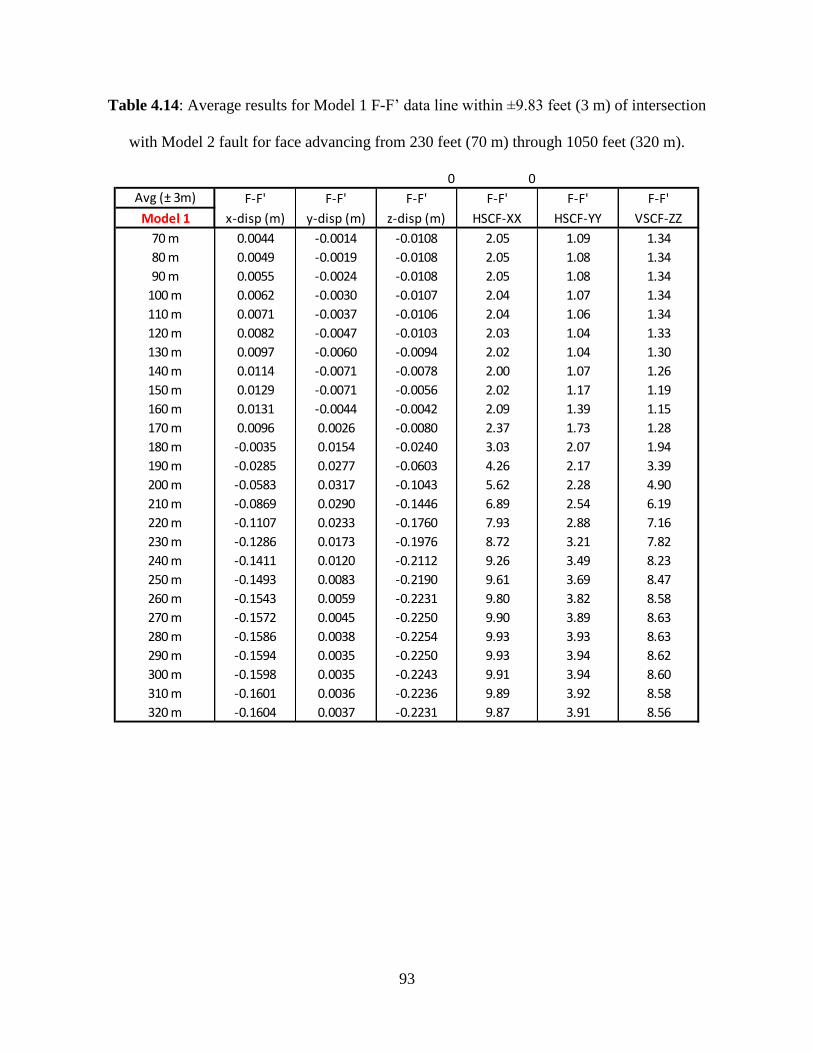
93

Table 4.14: Average results for Model 1 F-F’ data line within ±9.83 feet (3 m) of intersection


0 0

Avg (± 3m) F-F' F-F' F-F' F-F' F-F' F-F'


70 m 0.0044 -0.0014 -0.0108 2.05 1.09 1.34

80 m 0.0049 -0.0019 -0.0108 2.05 1.08 1.34

90 m 0.0055 -0.0024 -0.0108 2.05 1.08 1.34

100 m 0.0062 -0.0030 -0.0107 2.04 1.07 1.34

110 m 0.0071 -0.0037 -0.0106 2.04 1.06 1.34

120 m 0.0082 -0.0047 -0.0103 2.03 1.04 1.33

130 m 0.0097 -0.0060 -0.0094 2.02 1.04 1.30

140 m 0.0114 -0.0071 -0.0078 2.00 1.07 1.26

150 m 0.0129 -0.0071 -0.0056 2.02 1.17 1.19

160 m 0.0131 -0.0044 -0.0042 2.09 1.39 1.15

170 m 0.0096 0.0026 -0.0080 2.37 1.73 1.28

180 m -0.0035 0.0154 -0.0240 3.03 2.07 1.94

190 m -0.0285 0.0277 -0.0603 4.26 2.17 3.39

200 m -0.0583 0.0317 -0.1043 5.62 2.28 4.90

210 m -0.0869 0.0290 -0.1446 6.89 2.54 6.19

220 m -0.1107 0.0233 -0.1760 7.93 2.88 7.16

230 m -0.1286 0.0173 -0.1976 8.72 3.21 7.82

240 m -0.1411 0.0120 -0.2112 9.26 3.49 8.23

250 m -0.1493 0.0083 -0.2190 9.61 3.69 8.47

260 m -0.1543 0.0059 -0.2231 9.80 3.82 8.58

270 m -0.1572 0.0045 -0.2250 9.90 3.89 8.63

280 m -0.1586 0.0038 -0.2254 9.93 3.93 8.63

290 m -0.1594 0.0035 -0.2250 9.93 3.94 8.62

300 m -0.1598 0.0035 -0.2243 9.91 3.94 8.60

310 m -0.1601 0.0036 -0.2236 9.89 3.92 8.58

320 m -0.1604 0.0037 -0.2231 9.87 3.91 8.56

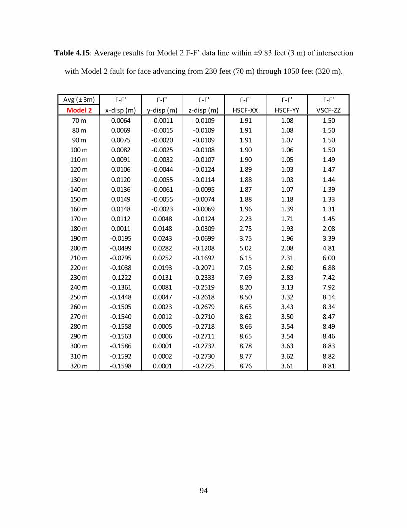
94

Table 4.15: Average results for Model 2 F-F’ data line within ±9.83 feet (3 m) of intersection




70 m 0.0064 -0.0011 -0.0109 1.91 1.08 1.50

80 m 0.0069 -0.0015 -0.0109 1.91 1.08 1.50

90 m 0.0075 -0.0020 -0.0109 1.91 1.07 1.50

100 m 0.0082 -0.0025 -0.0108 1.90 1.06 1.50

110 m 0.0091 -0.0032 -0.0107 1.90 1.05 1.49

120 m 0.0106 -0.0044 -0.0124 1.89 1.03 1.47

130 m 0.0120 -0.0055 -0.0114 1.88 1.03 1.44

140 m 0.0136 -0.0061 -0.0095 1.87 1.07 1.39

150 m 0.0149 -0.0055 -0.0074 1.88 1.18 1.33

160 m 0.0148 -0.0023 -0.0069 1.96 1.39 1.31

170 m 0.0112 0.0048 -0.0124 2.23 1.71 1.45

180 m 0.0011 0.0148 -0.0309 2.75 1.93 2.08

190 m -0.0195 0.0243 -0.0699 3.75 1.96 3.39

200 m -0.0499 0.0282 -0.1208 5.02 2.08 4.81

210 m -0.0795 0.0252 -0.1692 6.15 2.31 6.00

220 m -0.1038 0.0193 -0.2071 7.05 2.60 6.88

230 m -0.1222 0.0131 -0.2333 7.69 2.83 7.42

240 m -0.1361 0.0081 -0.2519 8.20 3.13 7.92

250 m -0.1448 0.0047 -0.2618 8.50 3.32 8.14

260 m -0.1505 0.0023 -0.2679 8.65 3.43 8.34

270 m -0.1540 0.0012 -0.2710 8.62 3.50 8.47

280 m -0.1558 0.0005 -0.2718 8.66 3.54 8.49

290 m -0.1563 0.0006 -0.2711 8.65 3.54 8.46

300 m -0.1586 0.0001 -0.2732 8.78 3.63 8.83

310 m -0.1592 0.0002 -0.2730 8.77 3.62 8.82

320 m -0.1598 0.0001 -0.2725 8.76 3.61 8.81

95

Table 4.16: Percent change on F-F’ within ±9.83 feet (3 m) of intersection with Model 2 fault




70 m 46 -25 1 -7 -1 11

80 m 41 -20 1 -7 -1 11

90 m 36 -17 1 -7 -1 11

100 m 32 -15 1 -7 -1 11

110 m 28 -13 1 -7 -1 11

120 m 29 -7 21 -7 -1 11

130 m 24 -8 21 -7 -1 11

140 m 19 -13 22 -7 0 11

150 m 15 -22 34 -7 1 12

160 m 13 -47 63 -7 1 14

170 m 16 86 56 -6 -1 13

180 m -133 -4 28 -9 -7 7

190 m -32 -12 16 -12 -9 0

200 m -14 -11 16 -11 -9 -2

210 m -9 -13 17 -11 -9 -3

220 m -6 -17 18 -11 -10 -4

230 m -5 -24 18 -12 -12 -5

240 m -4 -33 19 -11 -10 -4

250 m -3 -44 20 -12 -10 -4

260 m -2 -62 20 -12 -10 -3

270 m -2 -73 20 -13 -10 -2

280 m -2 -86 21 -13 -10 -2

290 m -2 -84 20 -13 -10 -2

300 m -1 -98 22 -11 -8 3

310 m -1 -94 22 -11 -8 3

320 m 0 -96 22 -11 -8 3

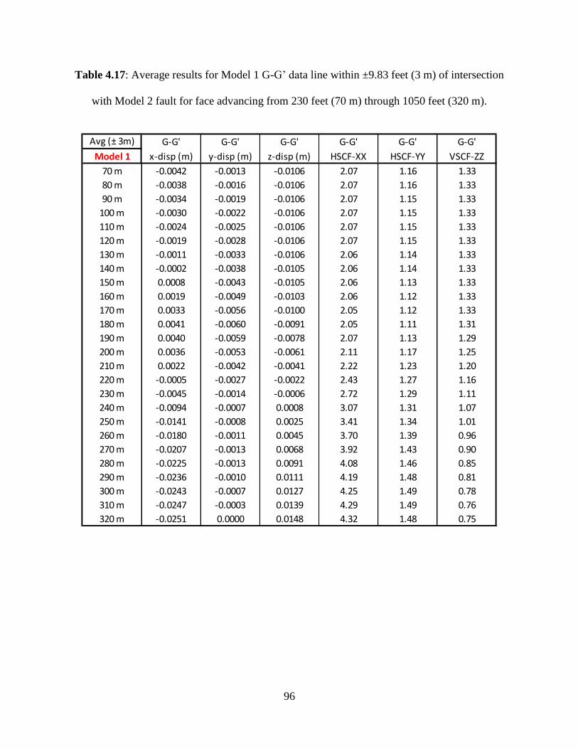
96

Table 4.17: Average results for Model 1 G-G’ data line within ±9.83 feet (3 m) of intersection


Avg (± 3m) G-G' G-G' G-G' G-G' G-G' G-G'


70 m -0.0042 -0.0013 -0.0106 2.07 1.16 1.33

80 m -0.0038 -0.0016 -0.0106 2.07 1.16 1.33

90 m -0.0034 -0.0019 -0.0106 2.07 1.15 1.33

100 m -0.0030 -0.0022 -0.0106 2.07 1.15 1.33

110 m -0.0024 -0.0025 -0.0106 2.07 1.15 1.33

120 m -0.0019 -0.0028 -0.0106 2.07 1.15 1.33

130 m -0.0011 -0.0033 -0.0106 2.06 1.14 1.33

140 m -0.0002 -0.0038 -0.0105 2.06 1.14 1.33

150 m 0.0008 -0.0043 -0.0105 2.06 1.13 1.33

160 m 0.0019 -0.0049 -0.0103 2.06 1.12 1.33

170 m 0.0033 -0.0056 -0.0100 2.05 1.12 1.33

180 m 0.0041 -0.0060 -0.0091 2.05 1.11 1.31

190 m 0.0040 -0.0059 -0.0078 2.07 1.13 1.29

200 m 0.0036 -0.0053 -0.0061 2.11 1.17 1.25

210 m 0.0022 -0.0042 -0.0041 2.22 1.23 1.20

220 m -0.0005 -0.0027 -0.0022 2.43 1.27 1.16

230 m -0.0045 -0.0014 -0.0006 2.72 1.29 1.11

240 m -0.0094 -0.0007 0.0008 3.07 1.31 1.07

250 m -0.0141 -0.0008 0.0025 3.41 1.34 1.01

260 m -0.0180 -0.0011 0.0045 3.70 1.39 0.96

270 m -0.0207 -0.0013 0.0068 3.92 1.43 0.90

280 m -0.0225 -0.0013 0.0091 4.08 1.46 0.85

290 m -0.0236 -0.0010 0.0111 4.19 1.48 0.81

300 m -0.0243 -0.0007 0.0127 4.25 1.49 0.78

310 m -0.0247 -0.0003 0.0139 4.29 1.49 0.76

320 m -0.0251 0.0000 0.0148 4.32 1.48 0.75

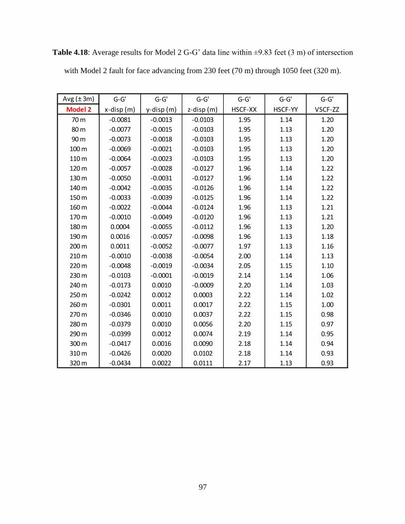
97

Table 4.18: Average results for Model 2 G-G’ data line within ±9.83 feet (3 m) of intersection




70 m -0.0081 -0.0013 -0.0103 1.95 1.14 1.20

80 m -0.0077 -0.0015 -0.0103 1.95 1.13 1.20

90 m -0.0073 -0.0018 -0.0103 1.95 1.13 1.20

100 m -0.0069 -0.0021 -0.0103 1.95 1.13 1.20

110 m -0.0064 -0.0023 -0.0103 1.95 1.13 1.20

120 m -0.0057 -0.0028 -0.0127 1.96 1.14 1.22

130 m -0.0050 -0.0031 -0.0127 1.96 1.14 1.22

140 m -0.0042 -0.0035 -0.0126 1.96 1.14 1.22

150 m -0.0033 -0.0039 -0.0125 1.96 1.14 1.22

160 m -0.0022 -0.0044 -0.0124 1.96 1.13 1.21

170 m -0.0010 -0.0049 -0.0120 1.96 1.13 1.21

180 m 0.0004 -0.0055 -0.0112 1.96 1.13 1.20

190 m 0.0016 -0.0057 -0.0098 1.96 1.13 1.18

200 m 0.0011 -0.0052 -0.0077 1.97 1.13 1.16

210 m -0.0010 -0.0038 -0.0054 2.00 1.14 1.13

220 m -0.0048 -0.0019 -0.0034 2.05 1.15 1.10

230 m -0.0103 -0.0001 -0.0019 2.14 1.14 1.06

240 m -0.0173 0.0010 -0.0009 2.20 1.14 1.03

250 m -0.0242 0.0012 0.0003 2.22 1.14 1.02

260 m -0.0301 0.0011 0.0017 2.22 1.15 1.00

270 m -0.0346 0.0010 0.0037 2.22 1.15 0.98

280 m -0.0379 0.0010 0.0056 2.20 1.15 0.97

290 m -0.0399 0.0012 0.0074 2.19 1.14 0.95

300 m -0.0417 0.0016 0.0090 2.18 1.14 0.94

310 m -0.0426 0.0020 0.0102 2.18 1.14 0.93

320 m -0.0434 0.0022 0.0111 2.17 1.13 0.93

98

Table 4.19: Percent change on G-G’ within ±9.83 feet (3 m) of intersection with Model 2 fault




70 m 94 -3 -3 -6 -2 -10

80 m 102 -4 -3 -6 -2 -10

90 m 115 -4 -3 -6 -2 -10

100 m 133 -5 -3 -5 -2 -10

110 m 161 -6 -3 -5 -1 -10

120 m 208 -2 20 -5 -1 -9

130 m 349 -4 20 -5 0 -9

140 m 1774 -7 20 -5 0 -9

150 m -516 -9 20 -5 0 -9

160 m -215 -11 20 -5 1 -9

170 m -131 -11 20 -4 1 -9

180 m -91 -9 23 -5 1 -9

190 m -60 -4 25 -5 0 -8

200 m -70 -3 26 -7 -4 -7

210 m -147 -10 32 -10 -7 -6

220 m 848 -31 55 -15 -10 -5

230 m 128 -92 218 -22 -12 -5

240 m 85 -234 -206 -28 -13 -3

250 m 72 -256 -90 -35 -15 0

260 m 68 -198 -61 -40 -17 4

270 m 67 -174 -46 -43 -20 9

280 m 68 -180 -39 -46 -22 13

290 m 69 -221 -33 -48 -23 17

300 m 72 -337 -29 -49 -24 20

310 m 72 -750 -26 -49 -24 22

320 m 73 -5558 -25 -50 -24 24

99

Table 4.20: Average results for Model 1 H-H’ data line within ±9.83 feet (3 m) of intersection


Avg (± 3m) H-H' H-H' H-H' H-H' H-H' H-H'


70 m -0.0055 -0.0009 -0.0121 2.05 1.10 1.38

80 m -0.0059 -0.0011 -0.0121 2.05 1.10 1.38

90 m -0.0063 -0.0013 -0.0121 2.05 1.10 1.38

100 m -0.0067 -0.0016 -0.0121 2.05 1.10 1.38

110 m -0.0072 -0.0019 -0.0121 2.05 1.09 1.38

120 m -0.0077 -0.0022 -0.0121 2.04 1.09 1.38

130 m -0.0084 -0.0025 -0.0121 2.04 1.09 1.38

140 m -0.0092 -0.0029 -0.0121 2.04 1.09 1.38

150 m -0.0101 -0.0033 -0.0121 2.03 1.08 1.38

160 m -0.0111 -0.0038 -0.0121 2.02 1.07 1.38

170 m -0.0123 -0.0043 -0.0120 2.01 1.07 1.37

180 m -0.0129 -0.0045 -0.0116 1.99 1.06 1.36

190 m -0.0129 -0.0045 -0.0109 1.98 1.05 1.34

200 m -0.0128 -0.0045 -0.0098 1.97 1.06 1.31

210 m -0.0125 -0.0043 -0.0083 1.98 1.07 1.27

220 m -0.0119 -0.0039 -0.0065 2.03 1.08 1.22

230 m -0.0109 -0.0034 -0.0044 2.13 1.09 1.16

240 m -0.0095 -0.0030 -0.0023 2.27 1.10 1.10

250 m -0.0080 -0.0027 0.0010 2.42 1.11 1.03

260 m -0.0067 -0.0026 0.0024 2.55 1.13 0.96

270 m -0.0060 -0.0023 0.0049 2.65 1.14 0.89

280 m -0.0056 -0.0020 0.0072 2.71 1.14 0.83

290 m -0.0055 -0.0015 0.0092 2.74 1.14 0.77

300 m -0.0054 -0.0010 0.0108 2.76 1.14 0.73

310 m -0.0054 -0.0005 0.0120 2.76 1.12 0.70

320 m -0.0052 -0.0002 0.0128 2.75 1.11 0.68

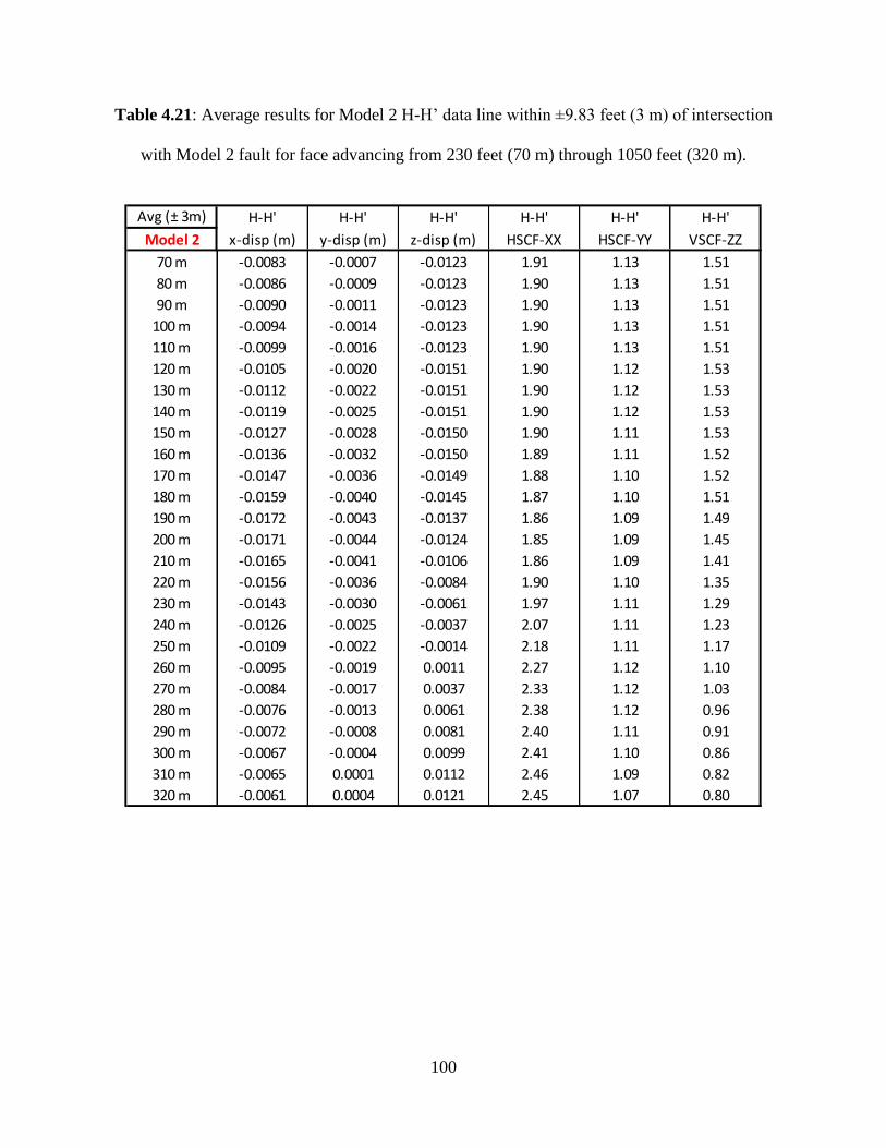
100

Table 4.21: Average results for Model 2 H-H’ data line within ±9.83 feet (3 m) of intersection




70 m -0.0083 -0.0007 -0.0123 1.91 1.13 1.51

80 m -0.0086 -0.0009 -0.0123 1.90 1.13 1.51

90 m -0.0090 -0.0011 -0.0123 1.90 1.13 1.51

100 m -0.0094 -0.0014 -0.0123 1.90 1.13 1.51

110 m -0.0099 -0.0016 -0.0123 1.90 1.13 1.51

120 m -0.0105 -0.0020 -0.0151 1.90 1.12 1.53

130 m -0.0112 -0.0022 -0.0151 1.90 1.12 1.53

140 m -0.0119 -0.0025 -0.0151 1.90 1.12 1.53

150 m -0.0127 -0.0028 -0.0150 1.90 1.11 1.53

160 m -0.0136 -0.0032 -0.0150 1.89 1.11 1.52

170 m -0.0147 -0.0036 -0.0149 1.88 1.10 1.52

180 m -0.0159 -0.0040 -0.0145 1.87 1.10 1.51

190 m -0.0172 -0.0043 -0.0137 1.86 1.09 1.49

200 m -0.0171 -0.0044 -0.0124 1.85 1.09 1.45

210 m -0.0165 -0.0041 -0.0106 1.86 1.09 1.41

220 m -0.0156 -0.0036 -0.0084 1.90 1.10 1.35

230 m -0.0143 -0.0030 -0.0061 1.97 1.11 1.29

240 m -0.0126 -0.0025 -0.0037 2.07 1.11 1.23

250 m -0.0109 -0.0022 -0.0014 2.18 1.11 1.17

260 m -0.0095 -0.0019 0.0011 2.27 1.12 1.10

270 m -0.0084 -0.0017 0.0037 2.33 1.12 1.03

280 m -0.0076 -0.0013 0.0061 2.38 1.12 0.96

290 m -0.0072 -0.0008 0.0081 2.40 1.11 0.91

300 m -0.0067 -0.0004 0.0099 2.41 1.10 0.86

310 m -0.0065 0.0001 0.0112 2.46 1.09 0.82

320 m -0.0061 0.0004 0.0121 2.45 1.07 0.80

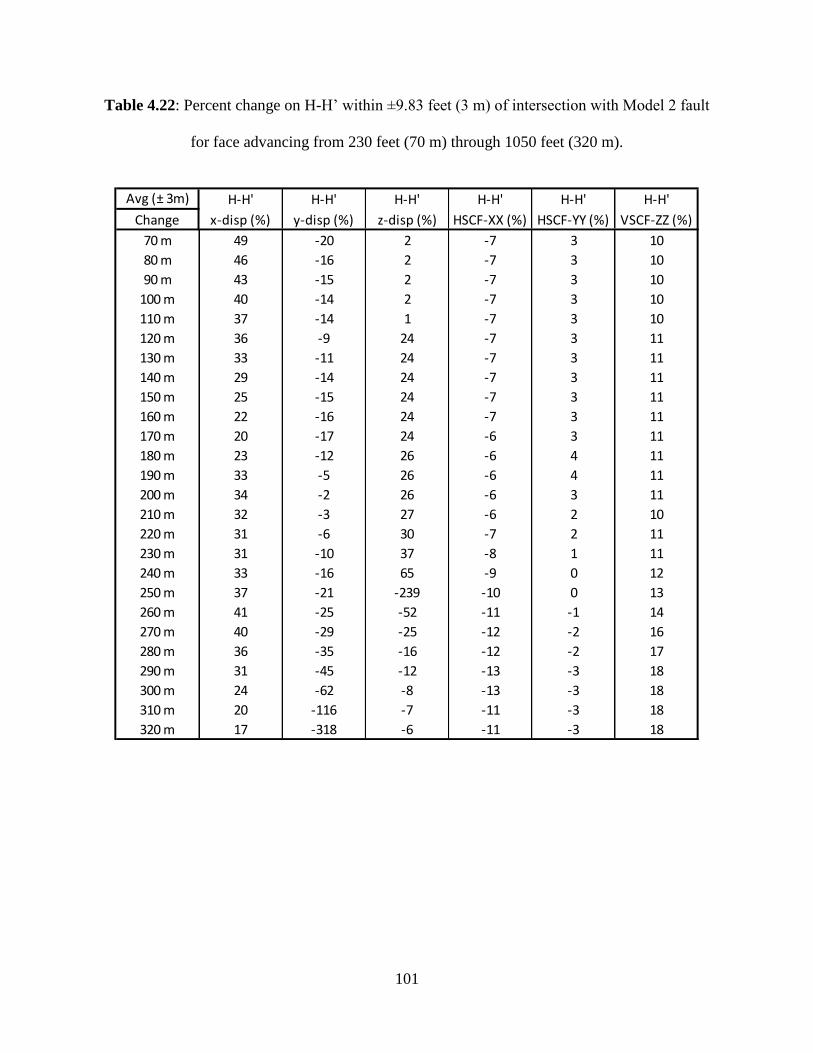
101

Table 4.22: Percent change on H-H’ within ±9.83 feet (3 m) of intersection with Model 2 fault




70 m 49 -20 2 -7 3 10

80 m 46 -16 2 -7 3 10

90 m 43 -15 2 -7 3 10

100 m 40 -14 2 -7 3 10

110 m 37 -14 1 -7 3 10

120 m 36 -9 24 -7 3 11

130 m 33 -11 24 -7 3 11

140 m 29 -14 24 -7 3 11

150 m 25 -15 24 -7 3 11

160 m 22 -16 24 -7 3 11

170 m 20 -17 24 -6 3 11

180 m 23 -12 26 -6 4 11

190 m 33 -5 26 -6 4 11

200 m 34 -2 26 -6 3 11

210 m 32 -3 27 -6 2 10

220 m 31 -6 30 -7 2 11

230 m 31 -10 37 -8 1 11

240 m 33 -16 65 -9 0 12

250 m 37 -21 -239 -10 0 13

260 m 41 -25 -52 -11 -1 14

270 m 40 -29 -25 -12 -2 16

280 m 36 -35 -16 -12 -2 17

290 m 31 -45 -12 -13 -3 18

300 m 24 -62 -8 -13 -3 18

310 m 20 -116 -7 -11 -3 18

320 m 17 -318 -6 -11 -3 18

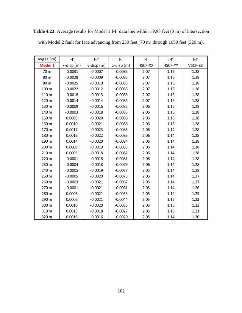
102

Table 4.23: Average results for Model 1 I-I’ data line within ±9.83 feet (3 m) of intersection


Avg (± 3m) I-I' I-I' I-I' I-I' I-I' I-I'


70 m -0.0031 -0.0007 -0.0085 2.07 1.16 1.28

80 m -0.0028 -0.0009 -0.0085 2.07 1.16 1.28

90 m -0.0025 -0.0010 -0.0085 2.07 1.16 1.28

100 m -0.0022 -0.0012 -0.0085 2.07 1.16 1.28

110 m -0.0018 -0.0013 -0.0085 2.07 1.15 1.28

120 m -0.0014 -0.0014 -0.0085 2.07 1.15 1.28

130 m -0.0009 -0.0016 -0.0085 2.06 1.15 1.28

140 m -0.0003 -0.0018 -0.0085 2.06 1.15 1.28

150 m 0.0003 -0.0020 -0.0086 2.06 1.15 1.28

160 m 0.0010 -0.0021 -0.0086 2.06 1.15 1.28

170 m 0.0017 -0.0023 -0.0085 2.06 1.14 1.28

180 m 0.0019 -0.0022 -0.0085 2.06 1.14 1.28

190 m 0.0014 -0.0020 -0.0084 2.06 1.14 1.28

200 m 0.0009 -0.0019 -0.0083 2.06 1.14 1.28

210 m 0.0003 -0.0018 -0.0082 2.06 1.14 1.28

220 m -0.0001 -0.0018 -0.0081 2.06 1.14 1.28

230 m -0.0004 -0.0018 -0.0079 2.06 1.14 1.28

240 m -0.0005 -0.0019 -0.0077 2.05 1.14 1.28

250 m -0.0005 -0.0020 -0.0073 2.05 1.14 1.27

260 m -0.0003 -0.0021 -0.0067 2.05 1.14 1.27

270 m -0.0001 -0.0021 -0.0061 2.05 1.14 1.26

280 m 0.0003 -0.0021 -0.0053 2.05 1.14 1.25

290 m 0.0006 -0.0021 -0.0044 2.05 1.15 1.23

300 m 0.0010 -0.0020 -0.0035 2.05 1.15 1.22

310 m 0.0013 -0.0018 -0.0027 2.05 1.15 1.21

320 m 0.0016 -0.0016 -0.0020 2.05 1.14 1.20

103

Table 4.24: Average results for Model 2 I-I’ data line within ±9.83 feet (3 m) of intersection




70 m -0.0060 -0.0007 -0.0083 2.01 1.15 1.17

80 m -0.0058 -0.0008 -0.0083 2.01 1.15 1.17

90 m -0.0055 -0.0009 -0.0083 2.01 1.15 1.17

100 m -0.0052 -0.0011 -0.0084 2.01 1.15 1.17

110 m -0.0048 -0.0012 -0.0084 2.01 1.15 1.17

120 m -0.0046 -0.0014 -0.0102 2.01 1.15 1.18

130 m -0.0041 -0.0015 -0.0102 2.01 1.15 1.18

140 m -0.0036 -0.0016 -0.0102 2.01 1.15 1.18

150 m -0.0030 -0.0018 -0.0102 2.01 1.15 1.18

160 m -0.0024 -0.0019 -0.0102 2.01 1.15 1.18

170 m -0.0018 -0.0020 -0.0102 2.01 1.15 1.18

180 m -0.0011 -0.0021 -0.0102 2.01 1.15 1.18

190 m -0.0005 -0.0021 -0.0101 2.01 1.15 1.18

200 m -0.0011 -0.0020 -0.0100 2.01 1.15 1.18

210 m -0.0020 -0.0019 -0.0099 2.01 1.15 1.18

220 m -0.0028 -0.0019 -0.0097 2.01 1.15 1.18

230 m -0.0033 -0.0019 -0.0094 2.01 1.15 1.18

240 m -0.0036 -0.0019 -0.0091 2.01 1.15 1.18

250 m -0.0037 -0.0019 -0.0086 2.01 1.14 1.18

260 m -0.0037 -0.0019 -0.0079 2.01 1.14 1.17

270 m -0.0036 -0.0019 -0.0070 2.01 1.14 1.16

280 m -0.0035 -0.0018 -0.0061 2.01 1.14 1.15

290 m -0.0033 -0.0017 -0.0050 2.01 1.14 1.15

300 m -0.0031 -0.0016 -0.0040 2.01 1.14 1.14

310 m -0.0028 -0.0013 -0.0030 2.00 1.13 1.13

320 m -0.0026 -0.0011 -0.0022 2.00 1.13 1.12

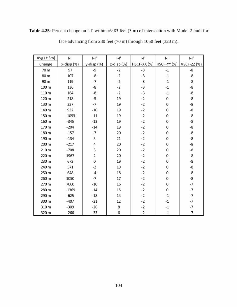
104

Table 4.25: Percent change on I-I’ within ±9.83 feet (3 m) of intersection with Model 2 fault for

face advancing from 230 feet (70 m) through 1050 feet (320 m).



70 m 97 -9 -2 -3 -1 -8

80 m 107 -8 -2 -3 -1 -8

90 m 119 -7 -2 -3 -1 -8

100 m 136 -8 -2 -3 -1 -8

110 m 164 -8 -2 -3 -1 -8

120 m 218 -5 19 -2 0 -8

130 m 337 -7 19 -2 0 -8

140 m 932 -10 19 -2 0 -8

150 m -1093 -11 19 -2 0 -8

160 m -345 -13 19 -2 0 -8

170 m -204 -14 19 -2 0 -8

180 m -157 -7 20 -2 0 -8

190 m -134 3 21 -2 0 -8

200 m -217 4 20 -2 0 -8

210 m -708 3 20 -2 0 -8

220 m 1967 2 20 -2 0 -8

230 m 672 0 19 -2 0 -8

240 m 571 -2 19 -2 0 -8

250 m 648 -4 18 -2 0 -8

260 m 1050 -7 17 -2 0 -8

270 m 7060 -10 16 -2 0 -7

280 m -1369 -14 15 -2 0 -7

290 m -625 -18 14 -2 -1 -7

300 m -407 -21 12 -2 -1 -7

310 m -309 -26 8 -2 -1 -7

320 m -266 -33 6 -2 -1 -7

105

4.3.2 Results Summary of Face Advance Analysis

For A-A’ and J-J’ data lines, analysis is done wherever the fault/face intersection occurs

for a given face advance location. As J-J’ moves with the advancing face, the intersection point

with A-A’ moves from being located in the block of coal to being located in gate entries after

623.4 feet (190 m). Summary comments for these data lines are as follows:


o Y-displacements, Z-displacements, and HSCF-XX changes become significant

between the two (2) models after 492 feet (150 m) of face advance. Supports

around the fault/face intersection should be increased as the face advances beyond

this point.

o The change in Y-displacement shifts repeatedly between positive and negative

values.

o The change in Z-displacement was positive after 656 feet (200 m) of face

advance.

o X-displacements, although relatively small, undergo significant change beyond

328 feet (100 m) of face advance and these changes between Models 1 and 2

tended to be more negative.

o HSCF-YY and VSCF are significant until approximately 800 feet (260 m) of face

advance. Typically, changes in HSCF-YY and VSCF-ZZ are almost always

negative between Models 1 to 2.

o The fault/face/gate intersection at 558 feet (170 m) of face advance is a critical

location for A-A’ X-displacements. For the next 66 feet (20m) of face advance

the most intense X-displacements along A-A’ for any advance location occur.

106


o Within the longwall panel, there is significant negative percent changes between

Models 1 and 2 for X-displacement, HSCF-YY, and VSCF-ZZ. Z-displacement

significantly increased in percent change after 623.4 feet (190 m) of face advance

where the analysis enters the gate entry.

o Along the face at the fault intersection HSCF-XX percentage change is usually

insignificant from Model 1 to Model 2.

o Changes in Y-displacement were only significant after J-J’ was measured in the

solid coal beyond the gate entries.

• Extra consideration for ground support should be taken as the face approaches the

location where the fault intersects each of the gate entries. Gate entry geometry

(including crosscuts) combined with an advancing face and a weak plane intersecting the

corner of a solid coal block to be mined by the longwall shearer creates a localized area

of low stiffness.

4.3.3 Results Summary of Gate Entry Analysis

Summary comments for the five (5) data lines in the gate entries are as follows:

• E-E’ data line

o X-displacement change increased significantly from 229.7 ft (70 m) to 393.7 feet

(120 m) of face advance, then decreased significantly until 623.4 feet (190 m) of

advance. Y-displacement change was significant and negative after 459.3 feet

(140 m) of face advance except when the face had advanced 525 feet (160 m)

107

where it was significant and positive. Change in Z-displacement were significant

and positive from 393.7 feet (120 m) to 558 feet (170 m).

o Percent change in HSCF-YY is significantly negative after 590.1 feet (180 m) of

face advance. The percent change is negative for HSCF-XX after 590.1 feet (180

m) of advance and significantly positive after 754.6 feet (230 m) of advance.

VSCF-ZZ significantly between positive and negative for face advancement from

492.1 (150 m) to 820.2 feet (250 m).

• F-F’ data line

o At the fault location, X-displacements increase significantly until the face passes

the intersection of F-F’ and the fault. At this point a significant decrease occurs

over the next 131 feet (40 m) of face advance. In both models, X- and Y-

displacements move in the positive X-direction and negative Y-direction until the

face passes by, at which point the direction of displacements move in the negative

X-direction and positive Y-direction. Changes in Y-displacement are consistently

and significantly negative after the face advances 230 feet (70 m). Significant

positive increases in Z-displacements occur after 304 feet (120 m) of face

advance.

o Changes in HSCFs were relatively insignificant until after 623 feet (190 m) of

face advance. VSCF significantly increases in the positive direction until 558 feet

(170 m).

• G-G’ data line

o X-displacement change is significantly positive both up to 459 feet (140 m) and

after 722 feet (220 m) of face advance. Between these distances, change is

108

significantly negative. Y-displacement changes are significantly negative after

492 feet (150 m) of face advance except when the face reaches the face/fault

intersection distance of 558 feet (170 m). Z-displacement changes are

significantly positive from 394 feet (120 m) to 755 feet (230 m) of face advance

and significantly negative thereafter.

o Changes in horizontal stress concentrations are significantly negative after 722

feet (220 m) of face advance.

• H-H’ data line

o X-displacement changes are significantly positive throughout face advancement.

Y-displacement changes are nearly entirely significantly negative. Z-

displacement changes are significantly positive from 394 feet (120 m) to 787 feet

(240 m) of face advance, and then significantly negative after.

o Changes in horizontal stress concentrations are not very significant. Changes in

VSCF are significantly positive throughout face advancement.

• I-I’ data line

o X-displacement changes are significantly positive except when the face (J-J’) is

within 115 feet (35 m) of the fault intersection with this data line, in which case

results are significantly negative. X-displacements are also significantly negative

after 919 feet (280 m) of face advance. Y-displacements are significantly

negative from 459 feet (140 m) to 558 feet (170 m) of face advance. Z-

displacements are significant and positive from 394 feet (120 m) to 984 feet (300

m) of face advance.

o No changes in SCFs were significant.

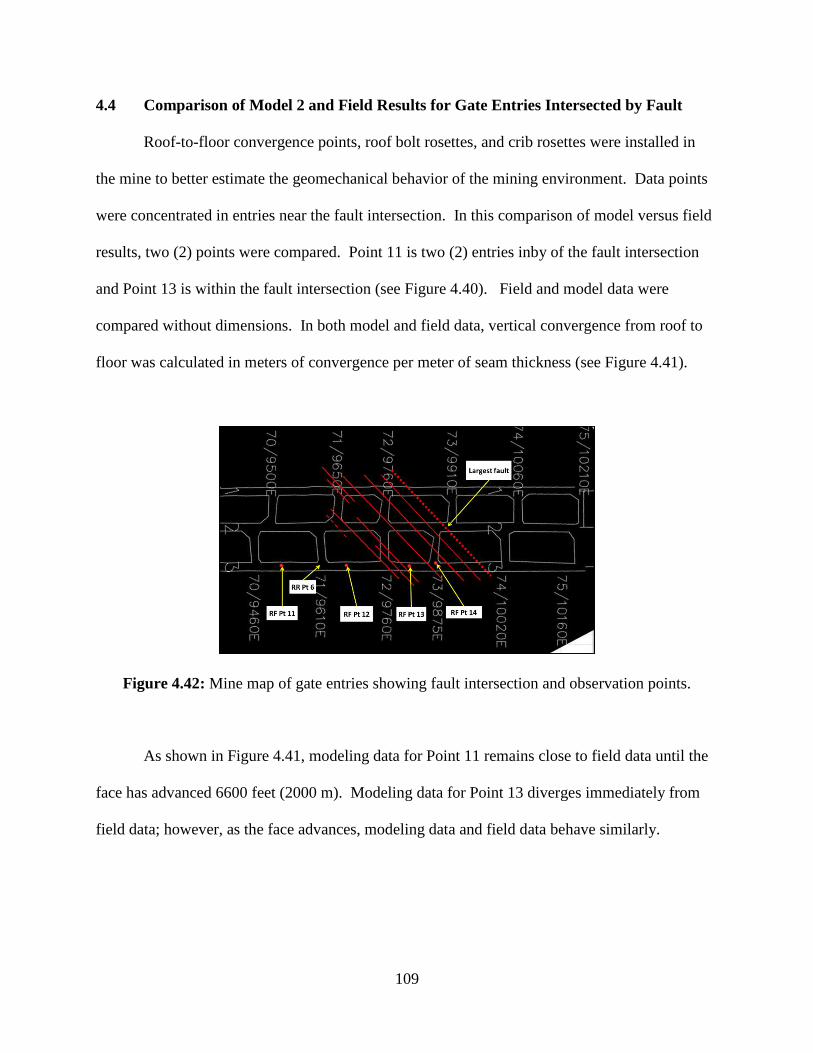
109

4.4 Comparison of Model 2 and Field Results for Gate Entries Intersected by Fault

Roof-to-floor convergence points, roof bolt rosettes, and crib rosettes were installed in

the mine to better estimate the geomechanical behavior of the mining environment. Data points

were concentrated in entries near the fault intersection. In this comparison of model versus field

results, two (2) points were compared. Point 11 is two (2) entries inby of the fault intersection

and Point 13 is within the fault intersection (see Figure 4.40). Field and model data were

compared without dimensions. In both model and field data, vertical convergence from roof to

floor was calculated in meters of convergence per meter of seam thickness (see Figure 4.41).

Figure 4.42: Mine map of gate entries showing fault intersection and observation points.

As shown in Figure 4.41, modeling data for Point 11 remains close to field data until the

face has advanced 6600 feet (2000 m). Modeling data for Point 13 diverges immediately from

field data; however, as the face advances, modeling data and field data behave similarly.

110

Figure 4.43: Points 11 and 13 results for model and physical mining environment.

There are several reasons for modeling data to not correspond closely to field data.

Models were generated for a study of macro-level behavior and the mesh was sized accordingly.

Natural mining environments are in a discontinuous environment where the model used a

continuum. The rock mass in the field would behave in a more confined manner than the

continuous media. In the field, multiple tight parallel faults were associated with the local

graben, whereas in the model a single weak plane was introduced. The heterogeneous nature of

the rock mass could have at least some influence in the difference of results. Models incorporate

regional stress values, but around the fault area, stress values could be much higher. Therefore,

at the micro-level within the model, data does not correlate strongly with data observed in the

field.

111

CHAPTER 5

CONCLUSIONS AND RECOMMENDATIONS

5.1 Summary of Research

This study has examined 3D stresses and displacements around a longwall mining system

that is intercepted by a geological fault. More specifically, the study analyzed the effect of a

fault on longwall gate development entries, set-up rooms, T-junctions, and the longwall face as

the longwall face progressed toward, through, and away from the fault. Linear 3D numerical

modeling was utilized for this purpose. A general lithologic sequence and mining parameters

related to the Herrin No. 6 coal seam in southern Illinois were employed within the model. Rock

mass engineering properties were developed for lithologic units associated with the coal seam

and used in analysis. The primary goal of this research was to develop a scientific understanding

of the effects of faults that can be used to guide the coal mining industry in providing a safe work

environment when they are present. A secondary goal was to develop recommendations for a

specific mining company to move through a geologic discontinuity without causing safety issues

or significant production loss.

FLAC3D code was used for simulating two (2) adjacent longwall faces. Linear elastic

rock mass elements with non-linear elastic-plastic fault elements were analyzed using Hoek-

Brown brittle failure criteria. Two (2) models were developed for analysis: a base elastic case

without faulting and an elastic model with elastic-plastic fault elements. Engineering properties

for the rock mass strata were derived from a history of rock core testing and modified following

the process indicated for Hoek’s Geologic Strength Index. Gob engineering properties and

estimated load carrying capacities developed in earlier studies were used to make simulations

112

physically realistic. The local tectonic (horizontal) stress field and vertical stress levels were

applied to the simulation boundaries.

Data was extracted from FLAC3D along several data lines in the roof and floor that were

determined to be critical based on the geometry of the mine layout. Extracted data included 3D

stresses and displacements with the Z-direction indicating vertical. This data was used to

calculate vertical convergence and stress concentration variables VSCF, HSCF-XX, and HSCF-

YY. Such data were developed for the longwall face advancing in 30-foot (10-m) increments

away from the set-up room.

5.2 Summary of Results

Overall, incremental displacements due to the presence of a fault are more significant

than stress concentrations related to the fault. Therefore, only displacement results are

summarized. It is important to note that observations made in this study are for the specific fault,

mining geometries, and engineering parameters used. Similar analyses must be performed using

site specific parameters to understand true effects.

5.2.1 Displacements in Areas where Fault Intersects Set-up Rooms

1. Incremental X-displacements (across the longwall face) around set-up rooms due to the

fault are generally small compared to displacements in the Y-direction (along the length

of the face) and the Z-direction (vertical).

2. Incremental X-displacements increase consistently in Model 2 by 31-37% in the front

row pillar/fault intersection and 2-16% in the second-row pillar/fault intersection.

113

3. Incremental Y-displacements around the first-row pillar/fault intersection in set-up rooms

are high (ranging from -26% up to 39%) when face advance begins, but reduce to almost

zero (0) after the face has advanced only 66 feet (20 m).

4. Z-displacements are similar in both models indicating little effect from faulting.

5. Horizontal and vertical stress concentrations are relatively unchanged due to the presence

of the fault.

5.2.2 Displacements in Areas where Fault Intersects Gate Development Entries

1. X-displacements (across the face) are small and decrease significantly in the model with

the fault until the face passes the area where the fault intersects gate development entries.

This is because of the arching effect around the weak fault zone.

2. Incremental Y-displacements (along gate entries) show large decreases (on a percentage

basis) around the intersection area as the longwall face advances towards it and away

from it, but a rapid increase (on a percentage basis) while the face is at the first gate

entry/fault intersection.

3. Z-displacements (vertical) increase significantly in all development entries around the

fault intersection zone for at least 200 feet (60 m) before and after the intersection area.

Displacements are small in entries further away from the intersection zone.

4. The effect of the fault is to decrease horizontal stress concentration in the gate entry/fault

intersection area due to vertical and horizontal deformations along the fault plane. First

row gate pillars at the fault experience a decrease in HSCF-XX and HSCF-YY ranging

from 7 to 13%. Second row gate pillars experience a decrease in HSCF-XX ranging from

6 to 13%. HSCF-YY remains relatively constant. Once the face passes by the fault

intersection area, horizontal stress concentrations are reduced to similar values found in

114

the model without faulting. This is over about 26 feet (8 m) along gate entry data lines.

5. VSCF values for gate development entry pillars are significantly increased around fault

intersection areas; however, these increases at the fault’s intersection with the first gate

row pillar cease after the longwall face passes by. Increases in VSCF at the second gate

row pillar/fault intersection are consistently 10-18%. Values rapidly normalize and are

similar to values in the model without faulting within 10 feet (3 m) on either side of the

gate development entry/fault intersection area.

5.3 Recommendations for Additional Research

1. This research modeled one (1) possible orientation and dip for a geologic anomaly.

Modeling additional fault orientations and dips as well as fault positioning with respect to

the longwall panel would show how the rock mass moves under different starting

conditions. This sensitivity study would reveal how stresses and displacements change in

different mining geometry environments.

2. Rock mass properties of the geologic anomaly are another important sensitivity variable.

Additional work needs to be done to ensure properties that are physically realistic.

3. Only one (1) panel was modeled in this study. Faults can go through multiple panels in a

mining environment and the size of a safe barrier pillar between panels needs to be

evaluated.

4. Except for the region around the fault, all elements were assigned elastic properties. Non-

linear analyses must be performed to assess these effects.

115

BIBLIOGRAPHY

Abbasi, B., Chugh, Y.P., and Gurley, H., 2014. “An Analysis of the Possible Fault

Displacements Associated with a Retreating Longwall Face in Illinois.” Proceedings, 48th

US Rock Mechanics/Geomechanics Symposium, 1-4 June, Minneapolis, MN, USA, 9 pp.

Beck, D., Reusch, F., Arndt, S., Thin, I., Stone, C., Heap, M., and Tyler, D., 2006. “Numerical

Modelling of Seismogenic Development during Cave Initiation, Propagation and

Breakthrough.” Deep and High Stress Mining 2006, 2-4 October, Quebec City, QC,

CAN, 15 pp.

Bieniawski, Z.T., 1984. Rock Mechanics Design in Mining and Tunneling. Balkema, Rotterdam,

NLD, 272 pp.

Board, M.P., Chacon, E., Varona, P., and Lorig, L., 1996. “Comparative Analysis of Toppling

Behaviour at Chuquicamata Open-Pit Mine, Chile.” Transactions – Institute of Mining

and Metallurgy, Vol. 105, Sec. A – Mining Industry, pp. 11-21.

Chen, J., Mishra, M., Zahl, E., Dunford, J., and Thompson, R., 2002. “Longwall Mining-induced

Abutment Loads and Their Impacts on Pillar and Entry Stability.” Proceedings, 21st

International Conference on Ground Control in Mining, 6-8 August, Morgantown, WV,

USA, pp. 11-17.

Chiu, C.-C., Wang, T.-T., Weng, M.-C., and Huang, T.-H., 2013. “Modeling the Anisotropic

Behavior of Jointed Rock Mass Using a Modified Smooth-joint Model.” International

Journal of Rock Mechanics & Mining Sciences, 62:14-22.

Chugh, Y.P., Gurley, H., Abbasi, B., Bastola, S., and Carlton, C., 2012. “Analysis and

Measurement of Ground Control Stability in Setup Rooms and Gate Roads in an Illinois

116

Longwall Operation.” Proceedings, Illinois Mining Institute Annual Meeting, 22-23

August, Marion, IL, USA, 50 pp.

Chugh, Y.P., Gurley, H., Abbasi, B., Carlton, C., Bastola, S., and Pulliam, J., 2013.

“Development and Field Demonstration of Alternate Stable Mining Geometries for Set-

up and Recovery Rooms in Illinois.” Final Technical Report for Illinois Clean Coal

Institute Project No. DEV11-5.

Clark, I., 2006. “Simulation of Rock Mass Strength Using Ubiquitous-joints.” Paper No. 08-07,

Proceedings, 4th International FLAC Symposium on Numerical Modeling in

Geomechanics, Hart, R. and Varona, P. (eds.), 29-31 May, Madrid, SPA.

Deb, D., Kumar, A., and Rosha, R.P.S., 2006. “Forecasting Shield Pressure at a Longwall Face

Using Artificial Neural Networks.” Geotechnical & Geological Engineering, Vol. 24,

Issue 4, pp. 1021-1037.

Dimitrakopoulos, R. and Li, S.X., 2010. “Quantification of Fault Uncertainty and Risk

Assessment in Longwall Coal Mining: Stochastic Simulation, Back Analysis, Longwall

Design and Reserve Risk Assessment.” Mining Technology, Transactions of the

Institutions of Mining and Metallurgy: Section A, Vol. 119, Issue 2, pp. 59-67.

Duplancic, P. and Brady, B.H., 1999. “Characterisation of Caving Mechanisms by Analysis of

Seismicity and Rock Stress.” Proceedings, 9th International Congress on Rock

Mechanics, Paris, FRA, G. Vouille and P. Berest (eds.), Vol. 2, CRC Press/Balkema,

Rotterdam NLD, pp. 1049-1053.

Frith, R., 2013. “A Holistic Examination of the Geotechnical Design of Longwall Shields and

Associated Mining Risks.” Proceedings, 2013 Coal Operators’ Conference, University of

Wollongong, 14-15 February, pp. 38-49.

117

Gale, W.J., 2004. “Rock Fracture, Caving and Interaction of Face Supports Under Different

Geological Environments: Experience from Australian Coal Mines.” Proceedings, 23rd

International Conference on Ground Control in Mining, 3-5 August, Morgantown, WV,

pp. 11-19.

Gale, W.J., 2005. “Application of Computer Modelling in the Understanding of Caving and

Induced Hydraulic Conductivity About Longwall Panels.” Proceedings, Coal2005

Conference, 26-28 April, Brisbane, QLD, pp. 11-15.

Hoek, E., Carranza-Torres, C., and Corkum, B., 2002. “Hoek-Brown Criterion – 2002 Edition.”

Proceedings, NARMS-TAC Conference, Toronto, ONT, CAN, Vol. 1, pp. 267-273.

Hoek, E., Marinos, P.G., and Marinos, V.P., 2005. “Characterisation and Engineering Properties

of Tectonically Undisturbed but Lithologically Varied Sedimentary Rock Masses.”

International Journal of Rock Mechanics & Mining Sciences, Vol. 42, pp. 277-285.

Holla, L. and Buizen, M., 1991. “The Ground Movement, Strata Fracturing and Changes in

Permeability Due to Deep Longwall Mining.” International Journal of Rock Mechanics

and Mining Sciences & Geomechanics, Vol. 28, Issues 2-3, pp. 207-217.

Hosseini, N., Oraee, K., and Gholinejad, M., 2010. “Design Optimization of Longwall Chain

Pillars.” Proceedings, 29th International Conference on Ground Control in Mining, 27-29

July, Morgantown, WV, USA, pp. 67-70.

Itasca Consulting Group (ITASCA), 2012. “Fast Lagrangian Analysis of Continua in Three-

dimensions Version 5.0.”

Kolebaevna, J.M., 1968. Theory of Ground Movement in Rock Mass (in Russian). Nedra,

Moscow, RUS, 101 pp.

Laubscher, D.H., 1994. “Cave Mining – The State of the Art.” Journal of South African

118

Institute of Mining and Metallurgy, Vol. 94, No. 10, pp. 279-293.

Lietner, R., Potsch, M., and Schubert, W., 2006. “Aspects on the Numerical Modeling of Rock

Mass Anisotropy in Tunneling.” Felsbau 24:2.

Marinos, P. and Hoek, E., 2000. “GSI: A Geologically Friendly Tool for Rock Mass Strength

Estimation.” Proceedings, GeoEng2000 International Conference on Geotechnical and

Geological Engineering, 19-24 November, Melbourne, AUS, International Society for

Rock Mechanics (ISRM), Lancaster, PA, USA, pp. 1422-1446.

Mark, C., Mucho, T.P., and Dolinar, D.R., 1998. “Horizontal Stress and Longwall Headgate

Ground Control.” Mining Engineering, Vol. 50, No. 1, pp. 61-68.

Martin, C.D., Kaiser, P.K., and McCreath, D.R., 1998. “Hoek-Brown Parameters for Predicting

the Depth of Brittle Failure around Tunnels.” Canadian Geotechnical Journal, Vol. 36,

No. 1, pp. 136-151.

Medhurst, T.P. and Reed, K., 2005. “Ground Response Curves for Longwall Support

Assessment.” Mining Technology, Transactions of the Institutions of Mining and

Metallurgy: Section A, Vol. 114, Issue 2, pp. 81-88.

Medhurst, T.P., Bartlett, M., and Sliwa, R., 2008. “Effect of Grouting on Longwall Mining

Through Faults.” Proceedings, Coal 2008: Coal Operators’ Conference, University of

Wollongong & Australasian Institute of Mining and Metallurgy, N. Aziz (ed.), pp. 44-55.

Nelson, W.J. and Krausse, H.-F., 1981. “The Cottage Grove Fault System in Southern Illinois.”

Illinois State Geological Survey, Circular 522, 71 pp.

Ozbay, U. and Rozgonyi, T.G., 2003. “Numerical Modeling of Stress and Deformations

Encountered in Deep Longwall Coal Mines Using Strain Softening Failure Criterion.”

Proceedings, International Conference on Safety and Environmental Aspects of Mining,

119

University of Miskolc, Vol. 63, pp. 123-135.

Peng, S.S. and Chiang, H.S., 1984. Longwall Mining. John Wiley & Sons, New York, NY, USA,

720 pp.

Pierce, M., Sainsbury, B.L., and Mas Ivars, D., 2009. “Use of Synthetic Rock Masses (SRM) to

Investigate Jointed Rock Mass Strength and Deformation Behavior.” Proceedings,

International Conference on Rock Joints and Jointed Rock Masses, 4-10 January, Tucson,

AZ, USA, 6 pp.

Pierce, M. and Lorig, L., 1998. “FLAC3D Analysis of Caveability of the Northparkes E26 Lift 2

Orebody.” Itasca Consulting Group, Inc. Report to Northparkes Mines, Parkes, NSW,

AUS, #1017, November.

Reyes-Montes, J.M., Sainsbury, B.L., Andrews, J.R., and Young, R.P., 2016. “Application of

Cave-Scale Rock Degradation Models in the Imaging of the Seismogenic Zone.” CIM

Journal, Vol. 7, No. 2, pp. 87-92.

Sainsbury, B.L., Pierce, M., and Mas Ivars, D., 2008. “Analysis of Caving Behavior Using a

Synthetic Rock Mass – Ubiquitous Joint Rock Mass Modeling Technique.” Proceedings,

1st Southern Hemisphere International Rock Mechanics Symposium (SHIRMS) , Vol. 1 –

Mining and Civil, Y. Potvin, J. Carter, A. Dyskin, and R. Jeffrey (eds.), Perth, AUS, pp.

243-254.

Sainsbury, B.L., Pierce, M., and Mas Ivars, D., 2008. “Simulation of Rock Mass Strength

Anisotropy and Scale Effects Using a Ubiquitous Joint Rock Mass (UJRM) Model.”

Proceedings, 1st International FLAC/DEM Symposium on Numerical Modeling, 25-27

August, Minneapolis, MN, USA,

Sainsbury, B.L., 2010. “Sensitivities in the Numerical Assessment of Cave Propagation.”

120

Proceedings, 2nd International Symposium on Block and Sublevel Caving, 20-22 April,

Perth, AUS, pp. 523-535.

Sainsbury, B.L., Sainsbury, D.P., and Pierce, M.E., 2011. “A Historical Review of the

Development of Numerical Cave Propagation Simulations.” Proceedings, 2nd

International FLAC/DEM Symposium on Numerical Modelling, 14-16 February,

Melbourne, AUS, 14 pp.

Sainsbury, B.L., 2012. A Model for Cave Propagation and Subsidence Assessment in Jointed

Rock Masses. Ph.D. Thesis, University of New South Wales, August.

Sainsbury, B.L. and Sainsbury, D.P., 2017. “Practical Use of the Ubiquitous-joint Constitutive

Model for the Simulation of Anisotropic Rock Masses.” Rock Mechanics and Rock

Engineering, Vol. 50, Issue 6, pp. 1507-1528.

Salamon, M.G.D., 1990. “Mechanism of Caving in Longwall Coal Mining.” Proceedings, 31st

US Symposium: Rock Mechanics Contributions and Challenges, 18-20 June, Denver,

CO, USA, Hustrulid, W.A. and Johnson, G.A. (eds.), Balkema, Rotterdam, NLD, pp.

161–168.

Salamon, M.D.G., 1991. “Displacements and Stresses Induced by Longwall Mining in Coal.”

Proceedings, 7th Congress of the International Society for Rock Mechanics, 16-20

September, Aachen, GER, Wittke, W. (ed.), Balkema, Rotterdam, NLD, pp. 1199-1202.

Salamon, M.D.G. and Munro, A.H., 1967. “A Study of the Strength of Coal Pillars.” Journal of

South African Institute of Mining and Metallurgy, 68:55-67.

Shabanimashcool, M. and Li, C., 2012. “A Numerical Study of Stress Changes in Barrier Pillars

and a Border Area in a Longwall Coal Mine.” International Journal of Coal Geology,

Vol. 106, February, pp. 39-47.

121

Thin, I.G.T., Pine, R.J., and Trueman, R., 1993. “Numerical Modelling as an Aid to the

Determination of the Stress Distribution in the Goaf Due to Longwall Coal Mining.”

International Journal of Rock Mechanics and Mining Sciences & Geomechanics

Abstracts, Vol. 30, Issue 7, pp. 1403-1409.

Trueman, R. and Mawdesley, C., 2003. “Predicting Cave Initiation and Propogation.” CIM

Bulletin, Vol. 96 (1071), pp. 54-59.

Trueman, R., Thomas, R., and Hoyer, D., 2011. “Understanding the Causes of Roof Control

Problems on A Longwall Face from Shield Monitoring Data – A Case Study.”

Proceedings, 11th Underground Coal Operators’ Conference, University of Wollongong

& Australasian Institute of Mining and Metallurgy, pp. 40-47.

Vakili, A., Albrecht, J., and Gibson, W., 2010. “Mine-scale Numerical Modelling of Longwall

Operations.” Proceedings, 2010 Coal Operators’ Conference, University of Wollongong

& Australasian Institute of Mining and Metallurgy, N. Aziz (ed.), pp. 115-124.

Verma, A.K. and Deb, D., 2007. “Analysis of Chock Shield Pressure Using Finite Element

Method and Face Stability Index.” Mining Technology (Trans. IMM A), 116(2), 67-78.

Verma, A.K. and Deb, D., 2008. “Numerical Analysis of the Interaction between Hydraulic

Powered Support and Surrounding Rock Strata at Indian Longwall Faces.” Proceedings,

12th International Conference of the International Association for Computer Methods and

Advances in Geomechanics (IACMAG), 1-6 October, Goa, IND, pp. 394-402.

Wang, T.T. and Huang, T.H., 2009. “A Constitutive Model for the Deformation of a Rock Mass

Containing Sets of Ubiquitous Joints.” International Journal of Rock Mechanics and

Mining Sciences, Vol. 46, No. 3, pp. 521-530.

Whittaker, B.N. and Reddish, D.J., 1989. Subsidence: Occurrence, Prediction, and Control.

122

Elsevier, Amsterdam, NLD, 528 pp.

Weir International, Inc. – WEIR, 2014. “United States Longwall Mining Statistics.” Annual

Report, 7 pp.

Yu, Z., Chugh, Y.P., Miller, P.E., and Yang, G., 1993. “A Study of Ground Behavior in

Longwall Mining through Field Instrumentation.” International Journal of Rock

Mechanics & Mining Sciences, Vol. 30, No. 7, pp. 1441-1444.

123

VITA

Graduate School

Southern Illinois University

Corbin Carlton

[email protected]

Southern Illinois University, Carbondale

Bachelor of Science, Mining Engineering, May 2012

Special Honors and Awards: Master Research Fellowship 2012-2015, SIU Carbondale

Thesis Title: An analysis of stresses and displacements around a fault plane due to longwall face

advance in coal mining

Major Professor: Yoginder P. Chugh

Publications:

• Chugh, Y.P., Gurley, H., Abbasi, B., Carlton, C., Bastola, S., and Pulliam, J., 2013.

“Development and Field Demonstration of Alternate Stable Mining Geometries for Set-

up and Recovery Rooms in Illinois.” Final Technical Report for Illinois Clean Coal

Institute Project No. DEV11-5.

• Bastola, S., Carlton, C., Abbasi, B., Chugh, Y. P. (2013) Stress distribution around

typical field intersection geometries in coal mines. Proc. of SME conf., Denver, USA.

• Chugh, Y. P., Gurley, H., Abbasi, B., Bastola, S., Carlton, C. (2012) Analysis and

measurement of ground control stability in setup rooms and gate roads in an Illinois

longwall operation” Illinois Mining Institute Annual Meeting, Illinois, USA

mailto:[email protected]

an analysis of stresses and displacements around a fault

Documents