An Analysis of the Characteristics of TemporaryEmployment in the Ecuadorian Labor Market: A

Microeconometric Study

MPP Professional Paper

In Partial Ful�llment of the Master of Public Policy Degree Requirements

The Hubert H. Humphrey School of Public A�airs

The University of Minnesota

José Luis Casco Guerra

May 5th, 2014

Signature below of Paper Supervisor certi�es successful completion of oral presentation and completion of�nal written version:

Dr. Deborah Levison Date, oral presentation Date, paper completion

Dr. Elizabeth Davis Date, oral presentation Date, paper completion

Dr. Yuhong Yang Date, oral presentation Date, paper completion

1 Introduction

Employment stability has been a widely discussed topic among Ecuadorian policy mak-

ers. In the last few decades Latin American economies have become increasingly volatile.

In response, many countries have enacted policies to increase the �exibility of their labor

markets, to mitigate the high levels of unemployment. These new contractual regulations

allowed �rms to hire employees with fewer employer liabilities and contract expiration or

dismissal costs. As Belot et al. (2002) explain, many reforms in the labor market produce

the intensi�cation of the use of contracts that foster low �ring costs. In Ecuador, labor �exi-

bility in Ecuador started to be implemented in 1990 with a legislation called Ley of Maquilas

(Factories Law).1 Subsequently, a whole body of new legislations was issued in the 1990s

and the beginning of 2000s, complementing the previous regulations, introducing new types

of �exible structures for hiring workers, in order to reduce unemployment (See Aguiar 2007).

As Blank and Freeman (1994) explain, the objective of changing the legal structure of labor

contracts is to diminish the e�ect of unemployment. Since the introduction of these em-

ployment structures, many employees have been hired under these types of contracts. Many

politician and policy makers, unions, employees and social sectors have argued against these

new �exible labor contracts claiming that they have negative consequences on the relative

stability of the workers and did not have signi�cant positive impacts on aggregate unem-

ployment and job quality. In 2008, the National Assembly of Ecuador decided to eliminate

many types of �exible labor contracts.

Consequently, the role of temporary contracts has increased interest and concern among

researchers and policy makers. In this context, it is necessary to identify and understand

the fundamental variables that characterize temporary employment, because as De Cuyper

et al. (2008) explain, the contractual structures have an e�ect not only on the employee's

side but also on the demand (�rms) side of the labor market. In this paper we study

the determinants of temporary contracts in the Ecuadorian labor market, as well as the

di�erences in the probability of men and women of obtaining this type of contract. As, Boeri

et al. (2005) explain, di�erent characteristics may determine the labor market behavior of

women. Therefore, it is necessary to study and understand the variables that in�uence

temporary employment in order to provide policy recommendations and contribute from an

academic perspective to the discussion of the Ecuadorian labor market structure.

Various methods help to explore the structure of temporary employment. We are go-

ing to undertake several analysis that use micro data, in order to identify the determinants

and the individual characteristics associated with temporary employment. Additionally, it

is important to analyze whether men and women have dissimilar motives for working un-

1Maquilas are manufacturing factories that operate in a free trade zones, under duty-free and tari�-free conditions.

2

der temporary contracts. As we are going to see in this analysis, men and women, indeed,

have di�erent reasons for engaging in temporary employment. There are diverse personal,

occupational, regional, and institutional reasons that in�uence this decision and it is neces-

sary to measure the impact of these characteristics in the probability of having a temporary

contract.

The organization of the paper is as follows. Section 2 presents a brief review of the

literature. Section 3 provides an overview of the characteristics of the Ecuadorian labor

market. Section 4 o�ers the description of the methodology underlying the empirical work

and describes the data set extracted from the ENEMDU. Section 5 presents the estimation

results. Finally, a succinct conclusion in Section 6 completes the paper.

2 A Brief Review of the Literature

In Ecuador, labor instability and underemployment has been a severe problem for the

last two decades. In this context, temporary employment has gradually become an impor-

tant topic in terms of the political and economic discussion. The increase in the use of

�exible contracts has been widely discussed in the literature. Uzzi et al. (1998) explain the

displacement and substitution of permanent employments with temporary employments in

United States and other industrialized countries. Booth et al. (2002) and the report of the

OECD (2002), devoted considerable attention to the analysis of contractual situations and

the e�ects on employees. The literature uses diverse methods to identify the main elements

that have an e�ect on temporary employment. Also, there are several perspectives to ex-

plain the factors that in�uence temporary employment. Many literature contributions that

explain the phenomenon of temporary employment concentrates on looking at the supply

side of the labor market. For example, Blosfeld et al. (2005) tries to elucidate the impact

of globalization and uncertainty in determining the employment stability. From the search

and match perspective of the labor market, globalization and technological progress have

an impact in this process by allowing job mobility and by providing di�erent employment

opportunities for the worker. However, these e�ects are mitigated due to higher competition

and uncertainty which induce people to keep their employments, increasing the job stability

and diminishing temporary employment (see also Auer 2005).The literature in this topic has also analyzed the role of institutional factors of a country.

Cebian et al. (2000) and Cahuk et al. (2001) explain how institutional factors or regulationsimpact the structure of temporary contracts. In the same perspective, Kahn (2007) tries toexplain how the employment protection reforms had an e�ect on temporary employment inEurope. These studies try to establish a relationship between formal institutions and tem-

3

porary employment.2 Other studies tried to investigate the e�ects that collective bargaining(unions) have on temporary employment. Several analyses demonstrate that unions play animportant role by generating a negative impact on the use of temporary employees (Uzzi etal., 1998; Olsen et al., 2004).3

On the other hand, several factors on the demand side of the labor market also have

an e�ect on temporary employment. Many studies analyze the cost structure of the �rms.

For instance, Houseman (2001) explain that lower costs4 are associated with temporary

employees, which in the framework of a pro�t maximizer �rm boosts the use of temporary

workers. Another interesting perspective from the demand side of the labor market is the

one presented by Uzzi et al. (1998). They explain the relationship between market structure

and temporary employment, �nding an increasing tendency to contract temporary employees

when �rms are facing growing markets. They argue that hiring temporary workers is a

strategy of the �rm to reduce costs and be competitive.There are several perspectives in the economic literature about the e�ects of labor �exibil-

ity on employment. For example, Bentolila et al. (1994) explain the e�ects of labor �exibilityon wages in Sapin, Blanchard et al. (2002) describe the e�ects on �xed duration contractdue to labor reforms in France, and Cahuc et al. (2002) explain the interrelation between theperformance of labor markets and temporary employment. Many authors also argue thatimplementing �xed-term contracts it is not a necessary condition to increase employment.Instead, the implementation of �xed-term contracts may lead to the creation of a dualism5

in the labor market. (Bentolila et al. 1994, Blanchard et al. 2002, Cahuc et al. 2002).6

Many researchers have argued about the importance of �xed-term contracts as a buildingblock on the path towards regular contracts with longer duration. However, there can bemixed employment e�ects due to the implementation of �xed-term contracts. The intro-duction of this type of contractual arrangement could raise dualism and limits the e�ectivemechanisms of workers to obtain a permanent employment. Güell (2000) explains the rela-tion between unemployment and �xed-term contracts from an e�ciency wage perspective,showing the consequences of implementing �xed-term contracts in an unaltered regulatoryframework.7

Several analyses in the literature showed how in many OECD countries, temporary em-

ployment has systematically gained ground. This type of job structure is currently present in

many labor markets, albeit permanent employment is the most desired form of contract. For

instance, there is an analysis of the situation of the labor market in Spain and its associated

2To further investigate the interplay of institutional factors, it is also important to review the works of Lindbeck et al.(2002), Scarpetta (1996) and Olsen et al. (2004).

3Another study that is in concordance with these conclusions is one conducted by Salladerre et al. (2007) for nineteenEuropean countries.

4Lower costs imply, for example, the absence of social security or smaller social security bene�t packages, precarious systemsof incentives and smaller wages. These lower costs for the �rms encourage the hiring of temporary workers.

5Dualism is a segmentation of the labor market into several distinct sub-labor markets e.g. formal and informal sectors.6Other interesting perspectives in this issue include: Aguirregabiria et al. (1999), Alonso-Borrego et al. (2002), Güell (2000)

and Saint-Paul (1996).7Güell (2000) argues that an economy achieves a lower employment equilibrium due to the e�ects of substituting �xed-term

for permanent contracts.

4

�exible regulatory framework. This study shows that implementing temporary employment

is a consequence of economic policies designed to foster labor �exibility and �rms' pro�ts

instead of employees' security and welfare (Dolado et al. 2002; Güell et al. 2007).

In contrast, other analyses o�er an explanation in favor of temporary contracts. For ex-

ample De Witte et al. (2003) explain the consequences of temporary work in job satisfaction

and organizational commitment in four European countries, and Engellande et al. (2005)

show that employees that work on a temporary basis tend to provide higher levels of e�ort

compared to permanent employees.8 These studies suggest that working on a temporary

basis does not imply poor working conditions or negative consequences for the employees.

They argue that positive results can be obtained by introducing temporary employment

schemes.

Some authors have tried to determine the characteristics of individuals who have tempo-

rary employment. It has been showed that employees who work under temporary schemes are

frequently younger individuals with lower levels of education and limited working experience

(see for instance, Russo et al. 1997; Hipple 2001; Valenzuela, 2003). Similar conclusions can

be encountered in the analysis conducted by Booth et al. (2000). Likewise, Salladarre et al.

(2007) obtained similar results in his analysis of the determinants of temporary employment

using the European Social Survey.There are several analyses that establish a linkage between �exible labor contracts and

female labor participation (Casey et al. 2004; Boeri et al. 2005; Hipple 2001; Salladerre etal. 2007). Other studies clarify the positive association between temporary employment andthe birth of a child and the e�ects of changing marital status (Wiens-Tuers et al. 2002; Boeriet al. 2005). In the framework of the unemployment duration, some studies have shown thatwhen unemployment takes place, the future probability of �nding an employment of longerduration decays. However, these studies also show that when a person has been unemployed,the probability of �nding temporary employment increases (See Chalmers et al. 2000; Guellet al. 2000).9

In Latin America and especially in Ecuador there is a lack of analyses to explore the

causes and consequences of temporary employment contracts. One analysis for Ecuador is

performed by Chavez et al. (2012) who analyze some of the characteristics that would make

it possible the existence of the �xed-term employment by branch of activity. However, as

Zelaschi (2007) explain, there have been some contributions towards answering some of the

questions regarding this area of research in other countries. Therefore, additional research is

needed to help scholars and policy makers better characterize temporary employment. This

paper tries to contribute to the understanding of temporary employment in the framework

of a small developing market economy.

8Similar results are exposed by Feldman (2005). Additional relevant studies in this area include Thorsteinson (2003) andMartin et al. (1995).

9A good discussion of these perspectives can be found in Booth et al. (2000) and Salladerre et al. (2007).

5

3 Characterizing the Fluctuations of the Ecuadorian Economy

A functional analysis that describes an economy should not assume ex-ante that a par-

ticular system behaves in a certain theoretical manner. Moreover, economic analysis of the

framework of Latin-American countries should be careful to consider complex situations of

uncertainty and turbulence in these economies. Therefore, an applied econometric analysis

have to start analyzing important stylized facts that an economy presents.10 In the perspec-

tive of Taylor (2004), empirical generalizations obtained should be understood as the result

of social relations over an empirical framework of social accountability. Moreover, to model

social relations and infer the e�ects of di�erent economic policies, it is of vital importance

to analyze the economic data of a country in a holistic way. This section will describe the

empirical characteristics of the Ecuadorian economy.

3.1 A brief overview of the Ecuadorian Economy

Commonly it is assumed that the level of real GDP is a good indicator of the quality

of life and welfare in an economy. In the context of real business cycles, GDP is the most

important component. It is known that in times of high economic growth (booms) living

standards of the population improve, there is less unemployment, increased production and

also higher consumption. Conversely, when the economy experiences recessionary times

conditions deteriorate.

To understand what is behind cyclical movements in the Ecuadorian economy it is neces-

sary to overview some historical and economic framework during the period of analysis. At

the beginning of the 1990s, the Ecuadorian economy took advantage of a stable international

environment characterized by high oil prices and the increase of exports of non-traditional

products. Moreover, the economy bene�ted from an increase in foreign direct investment

which incentivized private activity and the restructuring of the external debt via the Brady

Plan. All of these situations are re�ected in the increase of GDP during these years.

Nevertheless, this situation was not sustainable and since 1997 national production has

shrank because of the powerful e�ects of the �El Niño phenomenon� which leads to a dra-

matically reduction in the productivity of many economic sectors. Additionally, the decline

in price levels, the insolvency of the �nancial system and macroeconomic instability a�ected

the performance of the Ecuadorian economy.

The economy of Ecuador at this point was very unstable and in 1998 the incumbent

10This vision is in concordance with the emphasis that a structuralism vision of the economy presents, mainly based onrealistic 'stylized facts' or empirical generalizations at macro, sectorial and micro level about the economy in the study (seeKaldor, 1963).

6

government was unable to prevent the rise of interest rates and the restriction of credit. The

result was an increase of the �scal de�cit and the deterioration of the trade balance, triggering

a high devaluation process of the national currency (see Naranjo 2005). In addition to these

issues, the e�ect of the Asian crisis and the fall of oil prices seriously a�ected the overall

national economy. In 1999, a forced bank holiday was decreed, which at that time sent an

image of an unstable �nancial system and triggered the loss of con�dence in the economic

agents. Additionally, this crisis was also generated by factors such as the deregulation of

the banking system, the in�uence of powerful groups on technical and political decisions,

and greater demands of international and multilateral credit institutions. This situation

produced consequences in the real sector of the economy evidenced by the negative e�ects

in employment, consumption, investment and imports.

In 2000, in order to mitigate the e�ects of the crisis, the government decided to dollarize

the economy. At that time, the Central Bank of Ecuador (BCE) �xed the exchange rate

to the U.S. dollar at 25,000 sucres.11 Since then, the newly adopted policies produced a

momentary stabilization. After this period of crisis, the economy started to grow again due

to the reactivation of production and the recovery of household consumption.These turbulent scenarios have produced structural changes in the labor market. Many

employment polices have in some way a�ected the stability of the workers and have promotedthe creation of several temporary employment contractual arrangements.12

It is important to remember that labor �exibility in Ecuador was formally introduced in

1990 with the Ley de Régimen de Maquila y Contratación Laboral a Tiempo Parcial-Ley 90 13

and other legal �gures for part time work contracts. The aim of this law was the increase of

employment by fostering technology transfer and the creation of new technology production

sectors. The employees who worked under this new labor structure were considered part of

the formal labor sector of the economy, even though they had less protection and job stability.

This law, in conjunction with other labor legislation, generated a volatile situation for workers

as the employers had the opportunity to terminate contracts with fewer responsibilities in

terms of compensation payments. Moreover, in 2000, the Ecuadorian governments issued two

laws in order to introduce the dollar as the legal tender and to promote the modernization

and privatization of the Ecuadorian economy. These two laws deepened the instability of the

of the workers by introducing other types of contracts to hire employees with less liabilities.14

The reforms introduced in these laws were considered essential as a way to ensure access to

11The sucre was the national currency of the Republic of Ecuador between 1884 and 2000 before the dollarization processthat took place on January 10th of 2000.

12Historically, many governments have proposed more labor �exibility, greater trade liberalization, privatization proposals,�nancial and exchange rate policies reforms and a tax reform. These have produced several e�ects in the labor market stability.

13�Maquilas� are certain type of manufacturing companies that operate in a free trade zones. See, Ley de Maquilas yContratación Laboral a Tiempo Parcial (1990) �Código del Trabajo�, Registro O�cial 493, Agosto, Título II (Maquila Law andLaw for Part-time Hiring (1990) "Labor Code", O�cial Journal 493, August, Title II) for the the body of the law.

14These two laws are the: Ley para la Transformación Económica del Ecuador (Law for the Economic Transformation of theEcuador) also known as Trole 1 and Ley para la Promoción de la Inversión y Participación ciudadana (Law for the Promotionof Investment and Citizen Participation) also known as Trole 2.

7

employment and to improve the competitiveness of domestic �rms. These reforms contribute

to the creation of, for example, the hourly basis contract, temporal contract and the eventual

employment contracts. This legislation also a�ected collective bargaining contracts, employee

bene�ts and changed the regulations for job termination compensations (See Aguiar, 2007).

Another important labor reform that increased labor instability and temporary contracts

was the tercerización (outsourcing). This �gure was initially introduced in the period prior

to the dollarization of the economy in 1998, and in the period between 2003 and to 2005 the

legislation was complemented and expanded. In Ecuador, this speci�c form of employing

manpower was abused and had dramatic growth, becoming the customary method of many

companies to hire personnel.

Since 2003, the path of the Ecuadorian economy, has been characterized by tortuous po-

litical instability. However, with controlled in�ation due to dollarization, a favorable scenario

arose, creating a partial stability that triggered higher investments that foster the industrial

and productive sectors. Moreover, since 2007 the economy has enjoyed high oil prices which

have raised oil exports, generating a greater contribution of the external sector to the GDP.

Also, �scal policy has become really important because of the inability to manipulate mone-

tary policy. In this context, since 2007 the Ecuadorian economy implemented an aggressive

investment policy in education, health and infrastructure. Even though some small crises

have hit the country, the economy has maintained stability. Moreover, the government has

become a key driver of the economy, fostering many productive activities as a complement

to the private sector. This has produced a relatively strong performance of the GDP.

In the context of the labor market, we have seen that in this period, positive legal reforms

have improved job quality. In 2006 a law called Ley de Intermediación Laboral (Labor

Intermediation Act) was enacted. This new regulatory framework produced several changes

in the labor market with the aim of increasing employee bene�ts and imposing stricter

controls on �rms that use outsourcing as a mean of contracting workers.

The proliferation of legal temporary contracts during the crisis a�ected the stability of

workers, creating discomfort among the population. As a response, in 2008 the National As-

sembly of Ecuador decided to abolish many types of labor �exibility. This reduced the use

of temporary contract workers. However many companies and employers maintain certain

type of temporary contracts as they are unable to provide stability to all the workers. In this

context, the economic and political history of Ecuador show that growth in labor market

opportunities has been based partially on the �exibility of working contracts.15 For these rea-

sons, the main purpose of this analysis is to examine the impact of di�erent characteristics

in determining the probability of obtaining a permanent versus a temporary employment

contract.16 Moreover, we want to determine to what extent these characteristics (demo-

15This labor market structure opposes to vision that employee productivity depends on motivation and stability in a job.16In the context of the Ecuadorian legislation, �xed term contracts are those made to meet the labor demand of employers or

8

graphic, economic activity, region, etc.) impact the probability of have a permanent or

temporary employment contract by gender. Finally, it is important to provide some policy

recommendations, in order to improve the performance of the Ecuadorian labor market.

3.2 Some Stylized Facts of the Ecuadorian Labor Market

This section provides a brief description of the evolution of some important variables ofthe Ecuadorian labor market in order to have a better perspective on the performance ofsome important indicators. In Figure 1, we can observe the overall employment situation inEcuador obtained from the data provided by the INEC. The lines represent the historicalevolution of full employment, underemployment and unemployment. First, we can observethe behavior of full employment. For the period from 2007 to 2013, we observe a positivetendency with an increase from 32.5% in the �rst quarter of 2007 to 53.27% in the fourthquarter of 2013 and an overall mean of 43.21% for the whole period.17

Now, in terms of underemployment, in Figure 1 we can observe that on the period 2007

to 2013 the rate had an average of 47.84%, with a declining tendency from 58.69% in the

�rst quarter of 2007 to 44.84% in the fourth quarter of 2013. Therefore, underemployment

is one of the main problems of the Ecuadorian labor market, as many workers are holding

part-time jobs despite desiring full-time jobs. Also, many workers are overquali�ed for the

requirements of the jobs that they are performing. Although some reforms in the labor

legislation and the dollarization of the economy have brought some economic stability, the

overall e�ect on the quality and stability of the work has not had a decisive e�ect in the

Ecuadorian labor market structure. In Figure 1, we can also see that average unemployment

rate for the period 2007 to 2013 is 6.49% and has a declining tendency from 8.8% in the

�rst quarter of 2007 to 5.03% in the fourth quarter of 2013. From Figure 1, we can observe

that on average for every 100 Ecuadorians of the economically active population, 6.5 of them

could not �nd a job in 2013.

Additionally, it is important to look the unemployment rate for men and women separately

during the period 2007 to 2013. We can observe from Figure 2 that from the �rst quarter

of 2007 to the �rst quarter of 2011, women are predominantly the group having higher

unemployment rates with a mean of 4%, compared to men who have a mean of 3.54% during

this period. However, from the second quarter of 2011 to the fourth quarter of 2013, we can

see that men tended to have higher unemployment rates with a mean of 2.65% compared

companies (public or private). The duration of this type of contract has to be at least one year and the duties of the work hasto be stable or permanent in nature. On the other hand, temporary contracts are those made to meet situational demands ofthe employers or companies, such as replacing sta� who is absent for vacation, sickness, maternity, leave and similar situations.Temporary contracts can also be used to meet increased demand for production or services on usual activities of the employer,in which case the contract may not be longer than one hundred eighty continuous or discontinuous days within a period of threehundred sixty �ve days. If the circumstance or requirement of the worker's services is repeated for more than two periods ofone year, the contract will become seasonal contract which is also a temporary structure.

17This percentage represents the number of people with full employment over the economically active population.

9

to a mean of 2.4 % of women. The implications of this are important in terms of the e�ect

that unemployment has on workers and their families. A long period of unemployment may

lead to a decrease in the self-con�dence of the unemployed, and may lead them to agree to

take temporary jobs with lower wages and sometime in precarious labor environments.To have a better perspective of the situation of the Ecuadorian labor market, it is also

important to compare the Ecuadorian unemployment rate with the unemployment rate ofother economies of the Latin American region and important international economies suchas United States and Germany. In Figure 3, we observe that in the last years Ecuador hasconsistently achieved low rates of unemployment compared to other countries. In the periodbetween 2009 and 2013 the unemployment rate of Ecuador is lower than economies suchas United States and Germany, and it is also lower than other Latin American countrieswith the exception of Brazil. However, we can observe that in 2013, Ecuador reached anunemployment rate even lower than Brazil. This supports the idea that Ecuador has im-proved the situation of its labor market however underemployment and job stability remainas important challenges.18

As Figure 4 shows, underemployment tends to be higher for men rather than for women.

We also see that there is a decreasing tendency in the underemployment rate and a reduction

in the gap between males and females. The underemployment rate from men rose from

32.97% in the �rst quarter of 2007 to 23.23% in the fourth quarter of 2013. We have a

similar situation for women with a reduction of the underemployment rate from 25.72% in

the �rst quarter of 2007 to 20.12% in the fourth quarter of 2013. Furthermore, the overall

mean underemployment rate for men between 2007 and 2013 is 25.45% and it is higher

compared to the overall mean underemployment rate for women which is 22.94%. Therefore,

we observe that in this period, the percentage of Ecuadoreans males employed in the informal

sector or who work on an occasional basis is higher than the Ecuadoreans females in the same

situation.

From Figure 5, we can see that economically active population (PEA) has constantly

risen over period between 2007 and 2013. On the other hand the working age population has

a constant pattern over the years.19 Now, in Figure 6 we see the participation rate, which is

the ratio between the economically active population and the working age population. This

ratio measures the degree of participation of the population in the labor market. We can

observe a decreasing tendency of the participation rate from 62.2% in the �rst quarter of

2007 to 53.5% in the fourth quarter of 2013. The mean of this ratio for the period comprised

between 2007 and 2013 was 57.6%.

In many countries, women are less likely than men to participate in the labor market, i.e.

to be employed or actively seeking work. As Figure 7 shows, in Ecuador the participation18Higher rates of underutilization of human capital in the Ecuadorian economy may produce complex economic and social

issues, e.g., loss of knowledge and skills, reduction in current and life-long income and job dissatisfaction.19The economically active population is comprised of persons who worked at least 1 hour in the reference week, or if they did

not work, were previously working (employed) or those that were available for work or were seeking to work (unemployed) andthe working age population comprises all the people that are 10 years old and older.

10

rates for females are lower than for males. The participation gap between men and women

has maintained a slightly divergent tendency with a di�erence of 14% in the �rst quarter of

2007 to a gap of 18.6% in the fourth quarter of 2013. Moreover, the overall mean of the gap

among men and women is 15.37% for the period between 2007 and 2013.

4 Methodology

The aim of the present analysis is to determine the factors that a�ect the probability thata person has temporary employment. In this context, it is necessary to explain the necessaryeconometric tools that help us to model people's behavior and choices. With the help ofthese models we are going to be able to identify characteristics that in�uence the probabilityof obtaining a temporary job.20

4.1 Data Sources and Construction of Variables

The data employed for this analysis was obtained from the Instituto Nacional de Estadís-

tica y Censos (INEC, or National Institute of Statistics and Censuses).21 For the present

analysis the Encuesta Nacional de Empleo, Desempleo y Subempleo (ENEMDU, or National

Survey on Employment, Unemployment and Underemployment for Ecuador) will be used.

The ENEMDU is a household survey conducted quarterly in urban areas. The questionnaire

collects personal (characteristic), labor and income information. In this paper, we included

only people that are 15 to 65 years old, since the Ecuadorian Law states the minimum age

for signing a labor contract is 15 years for all types of work. The age range is also bounded

at 65 years old, as this is minimum age at which employees are able to retire. In the sample

we considered the last observation of an individual that appears in di�erent time periods.

The representative nationwide sample is taken from the second quarter of 2007 to the fourth

quarter of 2013. After cleaning the variables and values that are not in the scope of this

study, the �nal sample comprised 428,070 people.

For the present study a set of control variables was selected to take into consideration

personal, institutional, occupational and geographical characteristics of the individuals, to

verify whether these are crucial when obtaining a temporary contract. The selection of inde-

pendent variables is based on previous studies that have been conducted in many countries.

To determine which independent variables best explain the dependent variable, we carried

out a series of sub-models, to avoid having biased statistical results. The identi�cation of

20For a more comprehensive description of the models used in this study, see Cameron and Trivedi (2005) and Greene (2012).21This is a governmental institution that provides reliable survey information for the situtation of the Ecuadorian labor

market.

11

temporary employment is based on possible answers to the question about the type of hiring

of the worker and complemented ex-ante with the question about the participation in the

labor force.

4.2 Discrete Choice and Random Utility Model

To understand the basic framework of discrete choice models it is necessary to understand

the idea of random utility models.22 In this context, the utility comparison for an individual

n is not a continuous increase or decrease in utility U, but a discrete comparison. In our

case, we have a binary choice, which is obtaining a temporary job or not, and therefore the

comparison is U(1; 0) to U(0; 1).

We are not able to observe the utilities of people that choose to work under temporary

contracts or other type of contracts. What we are able to observe are the individual choices of

job. So, in this setting, the choice has a probabilistic component. Therefore, the alternatives

i (in case of having a temporary contract) and j (in case of having a non-temporary contract)

for an individual n is given by:

Pn(i) = Pr(Uin > Ujn) and Pn(j) = 1− Pn(i)

As we have individual di�erences and observational problems, we cannot assume a deter-

ministic relationship between the choices we observe and the values of U. In this context, it

is important to distinguish between systematic and random components of U. So we have

that:

Uin = Vin + εin and Ujn = Vjn + εjn

In the previous expression Vin represents the systematic or non-random component of

the utility of obtaining a temporary job and εin represents the stochastic component of the

utility of obtaining a temporary job. In the same context, Vjn represents the systematic or

non-random component of the utility of obtaining a non-temporary job and εjn represents

the stochastic component of the utility of obtaining a non-temporary job. Then, we have

that:23

22The treatment of discrete choice modeling, emphasizing the random utility model approach is much like the structuresuggested by McFadden (1981).

23 Let's substitute the last expression into the probability expression: Pn(i) = Pr[Vin + εin ≥ Vjn + εjn]= Pr[εin − εjn ≥Vjn − Vin]= Pr[εjn − εin ≤ Vin − Vjn]. Now, let εn = εjn − εin. Thus: Pn(i) = Pr[εn ≤ Vin − Vjn]

12

Pn(i) = Pr[εn ≤ Vin − Vjn]

A simple interpretation of this expression is that the probability that an individual n

chooses to work under a temporary contract equals the probability that the random ad-

vantage of obtaining a non-temporary job over obtaining a temporary job is less than the

systematic advantage of obtaining a temporary job over obtaining a non-temporary job.

This derivation is very important to understand discrete variable models. It is possible

to intuitively think of the di�erence between Vin and Vjn as a weighted combination of

the di�erent determinants between working under temporary contract and working under

a non-temporary contract. We can map this onto a real line. For instance, assume that

ε ∼ N(0, σ2). Now map the probability that εn is less than that number:

Vjn − Vin →∞, P r[εn ≤ Vin − Vjn]→ 1

Vin − Vjn → −∞, P r[εn ≤ Vin − Vjn]→ 0

This expression basically express the following relationship:

If Vin � Vjn, Pn(i)→ 1

If Vin � Vjn, Pn(i)→ 0

4.3 Linear Probability Model

In �gure 8(a), we can observe the decision structure of the linear probability model as well

as the Logit and Probit models.24 For this type of models the variable y has a qualitative

meaning with two possible outcomes:

y =

1

0

in case of having a temporary contract

in case of having a non− temporary contract

So we start with a multiple regression model:

y = β0 + β1x1 + . . .+ βkxk + µ

In this speci�cation we have that y is the endogenous variable, and x1, . . . xk are as set

of personal, labor, institutional and regional characteristics that in�uence the contractual

24We have based the discussion of Logit and Probit models in the treatment provided in many standard texts such as Greene(2012) or Cameron and Trivedi (2005). Good discussion in the theory and application of these models s can be found inAmemiya (1981, 1985), McFadden (1984) and Maddala (1983).

13

status of an individual and µ is and identically and independent distributed error. However,

it is important to mention that y has a quantitative meaning in thie linear probability model

structure. In this context, the discrete dependent variable is treated like a metric variable

and therefore we are able to use a common OLS regression methodology.

4.3.1 Parameter interpretation

Since y can take only two values, βj can be interpreted as a marginal e�ect of xj, therefore

it holds that:

E[y | x] = β0 + β1x1 + . . .+ βkxk

as well as

E[y | x] = P [y = 1 | x] = 1 ∗ P (y = 1 | x) + 0 ∗ (1− P [y = 1 | x])

and we can say that response probability corresponds to conditional expectation of y.

From the equations above we have that:

P [y = 1 | x] = β0 + β1x1 + . . .+ βkxk

Response probability p(x) = P [y = 1 | x] is a linear function of xj and the same applies

to P [y = 0 | x] = 1 = P [y = 1 | x]. Therefore, we have that βj measures the ceteris paribus

change of the response probability based on a one-unit change of xj:

∆P [y = 1 | x] = βj∆xj

In our case we can say that an additional unit in one of the characteristics has a marginalimpact βj on the probability of working under temporary employment, holding everythingelse constant.

4.3.2 Problems

When applying OLS, p(x) can take on values beyond the interval of [0, 1] and therefore theinterpretation as probability is implausible.25 Also, this model assumes identical increasesof probability when exogenous variables increase, independent of the actual level. Moreover,there are also problems of heteroscedasticity and µi can take only two values: −x′iβ and1− x′iβ:

E[µi] = P (1− x′iβ) + (1− P )(−x′iβ) = 0

25Furthermore, we have that linearity is implausible especially at the margins of realizations.

14

V ar[µi] = P (1− x′iβ)2 + (1− P )(−x′iβ)2

V ar[µi] = P (1− P ) = (x′iβ)(1− x′iβ)

βj are unbiased but standard errors are incorrect and therefore t-statistics and F-statisticsare not applicable. Consequently, we need to employ other types of models that take intoaccounts these nonlinearities.

4.4 Logit Model

We have already identi�ed the two main groups of workers (temporary and non-temporary),

therefore we need to apply a methodology that reveals the probability of being a temporary

employee based in some underlying characteristics. To assess the probability of having a

temporary job we are going to use a Logit regression model.26 This is a type of the binary

response model family that help us to correct some of the problems of the linear probability

model. In the Logit model the conditional probability has a structure given by:

p = Λ(x′iβ) =

exp(x′iβ)

1+exp(x′iβ)

and Λ(.) is the logistic distribution function and x′i are the vector of characteristics that

in�uence the contractual status of an individual. Therefore, it holds that:

p = Λ(z) = exp(z)1+exp(z)

= 11+exp(−z)

In order to �nd the desired parameters we need to obtain the �rst order condition of the

Logit-Maximum-Likelihood-Estimator:

N∑i=1

[yi − Λ(x′

iβ)]xi = 0

4.4.1 Marginal E�ects

In this model, estimated coe�cients do not re�ect marginal e�ects on probability as inthe linear probability model. Thus, it is useful to de�ne the marginal e�ect of a change of aregressor on the conditional probability for y = 1 as:

∂P [y=1|x]∂xij

= F′(x′iβ)βj

26For further discussion see Amemiya (1981, 1985), McFadden (1984) and Maddala (1983).

15

which depends on the value of the vector of characteristics xi, like in all non-linear models.

If we want to be more speci�c we can say that marginal e�ects in the Logit model can easily

be de�ned with the help of the coe�cients as:

∂pi∂xij

= pi(1− pi)βj with p = Λi = Λ(x′iβ)

For a rough estimate the following de�nition is helpful to specify that pi = y, that is to

say y(1− y)βj.

4.4.2 Odds Ratio

Often the e�ects of the reggresors are determined by the so-called odds ratio. The oddsratio describes the relative risk of probability for y = 1 and y = 0. We can say that theLog-odds ratios can be interpreted as semi-elasticities:

p =exp(x

′iβ)

1+exp(x′iβ)

p1−p = exp(x

′iβ)

ln p1−p = x

′iβ

Consequently, the odds ratio is a relative measures of the e�ect of one of the character-istics on the probability of obtaining a temporary versus non temporary contract, holdingeverything else constant.

4.5 Probit Model

To quantify the e�ect of the set of characteristics that in�uence the probability of havinga temporary employment, a Probit model is also speci�ed. This is another type of binaryresponse model. In the Probit model the conditional probability is:

p = Φ[x′iβ] =

´ x′iβ−∞ φ(z)dz

and Φ(z) is the distribution function of the standard normal distribution with the density

function φ(z) = 1√2π

exp(−z2

2) and x

′i are the vector of characteristics that in�uence the

contractual status of an individual. Again, in order to �nd the desired parameters we need

to obtain the �rst order condition of the Probit-Maximum-Likelihood-Estimator:

N∑i=1

wi[yi − Φ(x′

iβ)]xi = 0

in this model the weight wi =φ(x′iβ)

Φ(x′iβ)[1−Φ(x

′iβ)]

varies over the range of observations.

16

4.5.1 Marginal E�ects

With this type of model we can specify the marginal e�ect of a change of a regressor onthe conditional probability for y = 1:

∂pi∂xij

= φ(x′iβ)βj

4.6 Model Choice and Model Comparison

The speci�cations aforementioned are going be estimated in order to compare the threemodels and decide which one is the best �t to assess the e�ect of the set of characteristicsthat in�uence the probability of having a temporary employment.There are usually only fewdi�erences between logit and probit models in empirical applications.The largest di�erencesoccur at the margins of the distribution (near probabilities of 0 or 1) but these are notcrucial with respect to average marginal e�ects of a sample. Model comparison is donewith confrontation of log-likelihoods and therefore the models produce considerably di�erentcoe�cients β. Additionally, we are going to the Akaike Information Criterion, or AIC, givenby Sakamoto, Ishiguro, and Kitagawa (1987) and the Bayes Information Criterion, or BIC,given by Schwarz (1978). In both measures, smaller values are preferred.

Also, it is important to establish the di�erences among the goodness of �t. Linear models

goodness of �t is measured with the help of R2:

R2 = 1−∑µi∑

(yi−y)2

by minimizing the squared residuals a maximization of goodness of �t is realized. However,

using R2 is di�cult in probit and logit models because computing µi = y∗i − y∗i is not possibleas y∗i cannot be observed. We have that maximum likelihood method has a di�erent target

function than OLS, which is maximizing the likelihood function rather than minimizing the

sum of squared residuals. Therefore a good approach to measure the goodness of �t in this

type of models is McFadden's R2MF , which draws on the value of the log-likelihood function.

A standardization is necessary since the absolute value of the log-likelihood is not meaningful:

R2MF = 1− LN (β)

LN (y)

R2MF = 1−

∑i{yi ln pi + (1− yi) ln(1− pi)}N [y ln y + (1− y) ln(1− y)

We have that LN(β) is the value of the log-likelihood function with ML-estimators of the

respective model and LN(y) is the log-likelihood function of the model with only an intercept

(β = 0). Additionally, we are going to use other R-squared measures, such as the R-squared

of Cragg-Uhler-Nagelkerke, in order to compare the di�erent speci�cations.

17

4.7 Fairlie's Method of Decomposition

To implement this methodology, it is necessary to initially identify the two subsets of

workers (temporary and non-temporary). After that we are able to execute various estima-

tion procedures to reveal the di�erences in the probability of obtaining a temporary contract

between men and women. To measure the probability of having temporary employment it

is appropriate to estimate a Logit/Probit model for all employed individuals. Subsequently,

an evaluation of the model is executed by adding interaction terms. This speci�cation in-

troduces new variables to the previous equation by multiplying each of the factors by the

female dummy. After that, we apply the Fairlie decomposition technique for the logit/probit

model in order to identify and quantify the contributions of gender di�erences.

Now, let's start by de�ning the initial models as:

P (Yi = 1) = F (β0 +Xiβ1 + Aiβ2 +Biβ3 + µ)

Yi - is a dichotomous variable that has a value of 1 if the employment is temporary or 0

if the employment is permanent.

β0, β1, β2, β3 � vectors of coe�cients

Xi - set of personal and family characteristics:

p Sex (Female, Male) [Reference category: Female]

p Age (Ranges:15-25, 26-35, 36-45, 46-55, 56-65) [Reference category: 36-45]

p Education (None, Primary, Secondary, Higher non-university, University, Gradu-

ate) [Reference category: University]

p Race (Indigenous, White, Black-Afro, Mestizo, Other, Montubio) [Reference cat-

egory: Mestizo]

p Marital Status (Married, Divorced/Separated, Single) [Reference category: Mar-

ried]

Ai - set of occupational characteristics:

p Category of Occupation (Government employee, Private employee, Outsourced,

Journeyman, Domestic employee) [Reference category: Government employee]

p Duration in a company (Less than one year, More than one year) [Reference

category: Less than one year]

p Size of company (Less than 100 employees, More than 100 employees) [Reference

category: Less than 100 employees]

p Working hours (Part time, Full time) [Reference category: Full time]

18

Bi - set of institutional and regional characteristics

p Government Cash Transfer (Yes, No) [Reference category: No]

p Regions (Sierra-Highlands, Coast, Amazon) [Reference category: Sierra-Highlands]

p Area (Urban, Rural) [Reference category: Urban]

The subsequent step is to estimate the aforementioned model speci�cation with additional

interaction terms. This new speci�cation introduces additional variables to the previous

equation. We are going to generate new terms by multiplying all variables in the previous

speci�cation by the dummy for sex Df (1 for female, 0 for male). Thus, we have the

speci�cation as:

P (Yi = 1) = F (β0 +Xiβ1 + Aiβ2 +Biβ3 +DfXiβ4 +DfAiβ6 +DfBiβ7 + µ)

With this speci�cation, we are able to observe the e�ects of the Sex dummy in the di�erent

factors that have been included in the regression equation.

To examine the gender di�erentials, a useful method is the Oaxaca-Blinder decomposition

method. The Oaxaca (1973) and Blinder (1973) methodology helps decompose the mean

di�erences in some outcome variables between two groups. This decomposition permits us to

identify a part which is due to di�erences in observable characteristics (explained di�erential)

and another part which is due to di�erences in unobservable characteristics (unexplained

di�erential). However, this technique of Blinder (1973) and Oaxaca (1973) involves coe�cient

estimates from linear regressions only and it is not possible to apply in this case, as our

outcome variable is binary. As we a have a logit/probit regression model with a binary

dependent variable, it is necessary to employ another type of methodology. Fairlie (1999,

2005) and Yun (2004) have proposed useful methodologies that help to obtain a detailed

decomposition when we are dealing with limited dependent variable models. Therefore,

in the present analysis, Fairlie's method of decomposing for logit/probit models is used to

obtain the di�erences among male and female. By applying this methodology, it is possible

to disentangle the gender di�erences of temporary versus permanent employment. The

speci�cation of the Fairlie decomposition is given by:

Y F − Y M = (Nf∑i=1

F (Xfi β

f )

Nf−

Nm∑i=1

F (Xmi β

m)

Nm) + (

Nf∑i=1

F (Xfi β

f )

Nf−

Nf∑i=1

F (Xfi β

f )

Nf)

F - cumulative distribution function from logistic distribution (logit model) or standard

normal distribution (probit model)

X - row vector of independent variables

19

β - vector of coe�cient estimates for Sex (Male, Female).

4.8 Selection Bias in Binary Choice Models

In the present study, we want to know how several characteristics a�ect the likelihood of

success of obtaining a temporary contract. The main problem is that information about the

contractual situations is only available for the people who have an employment.

In order to solve this selection problem,27 we are going to �rst use a multinomial logit

model, which takes into consideration not only the people who are working, but also the

people who are not working. Also a useful tool, when we are dealing with selection, is the

Heckman model (see Heckman, 1979). However, this type of model has the limitation that

the outcome equation should involve a continuous dependent variable. In the present study,

we are interested in estimating an outcome equation that involves a dichotomous dependent

variable. In this context, we deal with a probit selection equation and a probit outcome

equation. Therefore, a bivariate probit model framework is an appropriate methodology in

this case.

4.8.1 Multinomial Logit

In �gure 8(b), we can observe the decision structure of the multinomial logit model.28 In

this case we infer that the decision of the person n that choose a labor status alternative j

is described by the utility equation,

Unj = Vnj + µnj

The systematic component of the utility function is given as,

Vnj = znγj

Therefore,

Unj = znγj + µnj

In the previous equation, γj is a vector of alternative-speci�c parameters. So, in this

type of speci�cation the e�ect of the regressors will vary across all the labor status choices.

27There is a variety of literature on models from selected samples. Good treatments are provided by Maddala (1983) andGouri'eroux (2000), Amemiya(1984, 1985) and Greene (2012).

28Amemiya (1981, 1985), Maddala (1983), Greene (2012), Ben-Akiva and Lerman (1985) and Train (1986) provide theoryand applications to understand the structure of multinomial models.

20

Consequently, we have that a person n that chooses a temporary contract alternative i, has

a probability:

Pni = exp{Vni}∑j exp{Vnj}

Pni = exp{znγi}∑j exp{znγj}

As in previous models this can be estimated using a log likelihood estimation process.

4.8.2 Bivariate Probit

In this type of model, we have a structure which is composed of two separate probit

models with correlated disturbances.29 This model, has an structure similar to the seemingly

unrelated regression models (SUR).30

In this context, we have two dichotomous dependent variables. By applying this type of

methodology we are basically trying to model two interrelated decisions of a person. In the

�rst stage we are interested in modeling if a person participates or not in the labor market

and in the second stage we are interested in whether the person chooses a temporary contract

or not. Moreover, we employ this type of model because we assume that the two decisions

are interrelated. In �gure 8(c), we can observe the decision structure of the bivariate probit

model. Thus, the model is given by

y∗1 = x1β1 + µ1

y∗2 = x2β2 + µ2

where the expressions y∗1 and y∗2 are unobservable latent variables that are linked to the

binary dependent variables y1 and y2 by

y1 =

1 if y∗1 > 0

0 if y∗1 ≤ 0and y2 =

1 if y∗2 > 0

0 if y∗2 ≤ 0

In this framework, it is important to note that if the errors are independent among the

two probit models, then it is possible to estimate these models separately. However, in our

case, we expect to have a covariance di�erent from zero and therefore we will have that

µ1i = ηi + ε1i29For further discussion of this model see Greene (2012) and Cameron and Trivedi (2005).30For a discussion of Seemingly Unrelated Regression models (SUR) see chapter 10 of Greene (2012).

21

µ2i = ηi + ε2i

This means that in each of the models the error is composed of an element εi exclusive

to that model and joint component ηi. As we are using a bivariate probit speci�cation we

assume that µji, εji and ηi for j = 1, 2, are normally distributed. This implies that µji is

in�uenced partially by ηi, which indicates that µ1i and µ2i are correlated. In this context,

we want to estimate the joint probability of y1i and y2i.31 So

P (y1i = 1) = P (µ1i > −x′1iβ)

= P (ε1i + ηi > −x′1iβ)

and

P (y2i = 1) = P (µ2i > −x′2iβ2)

= P (ε2i + ηi > −x′2iβ2)

The joint probability of several random variables is the product of their marginal prob-

abilities, if these random variables are independent. However, in our case the two random

variables are not independent and therefore we need to �nd the joint probabilities for non-

independent events. Thus,

P (y1 = 1, y2 = 1) = P (y1 = 1|y2 = 1)× P (y2 = 1)

= P (y1 = 1)× P (y2 = 1|y1 = 1)

In order to obtain this probability we will use a bivariate normal distribution.32 For the

estimation of the bivariate probit model we are going to assume that the errors are i.i.d.

following a standard bivariate normal distribution with correlation ρ (which can be also

expressed as µ1, µ2 ∼ φ2(0, 0, 1, 1, ρ)).33

This methodological structure helps us to obtain the necessary probabilities, as for exam-

ple, the probability of going to the labor market and having a temporary employment,

31In the case in which ρ = 0, we can estimate independently the two probit equations and obtain consistent results. But,when we have a ρ 6= 0, it is better to estimate the two equation jointly, as it is more e�cient.

32

The bivariate normal distribution is φ2 = φ(µ1, µ2) = 1

2πσµ1σµ2

√1−ρ2

exp[− 12

(µ21+µ

22−2ρµ1µ2

1−ρ2 )], where the correlation

coe�cient ρ represents the degree of association of the errors µ1 and µ2. Their joint cdf is given

byΦ2 = Φ(µ1, µ2) =´µ1

´µ2φ(µ1, µ2, ρ)dµ1dµ2

33 Consequently, E[µ1|x1, x2] = E[µ2|x1, x2] = 0;Cov[µ1|x1, x2] = Cov[µ2|x1, x2] = 0;Cov[µ1, µ2|x1, x2] = ρ

22

P (y1i = 1, y2i = 1) =´ µ1i−∞

´ µ2i−∞ φ2(x1β1, x2β2; ρ)dµ1dµ2

= Φ(x1β1, x2β2; ρ)

Similarly as in the previous models, in order to �nd the desired parameter, we need to

obtain the Maximum-Likelihood-Estimator. In the case of the bivariate probit model, the

log-likelihood is a sum across the four possible combinations of y1 and y2 multiplied by their

associated probabilities. Therefore, the the log-likelihood for the bivariate probit model is

given by

lnL =N∑i=1

{y1iy2iΦ2(x1β1, x2β2; ρ) + y1i(1− y2i)ln[Φ(x1β1)− Φ2(x1β1, x2β2; ρ)]

+(1− y1i)y2iln[Φ(x2β2)− Φ2(x1β1, x2β2; ρ)

+(1− y1i)(1− y2i)ln[1− Φ(x1β1)− Φ(x2β2)− Φ2(x1β1, x2β2; ρ)]

4.8.3 Marginal E�ects

Again, as in previous models, in the bivariate probit case, it is possible to obtain the

marginal e�ect of a change of a regressor. However, in the case of a bivariate probit model,

we are interested in the conditional mean function,

E[y1|y2 = 1] = P (y1 = 1|y2 = 1) = P (y1=1,y2=1)P (y2=1)

= Φ2(x1β1,x2β2;ρ)Φ(x2β2)

And then we can take the derivative of this expression with respect to any of the regressors

in order to get the marginal e�ects.

5 Results of the model

5.1 Descriptive Analysis

It is important to perform an exploratory analysis to determine the structure and quality

of the database. Here, we present the �nal results of the main variables used for the estima-

tion process. We start the analysis by exploring the main features of the variables employed

in the study. This will provide a good insight into the situation of the Ecuadorian labor

market. Several tables are presented in order to show the distributional characteristics, as

well as, the structure of important variables that a�ect a person's contractual situation. By

23

examining these descriptive statistics, we are able to identify some of the features related

to the probability of having a temporary versus other type of contractual situations. Before

we start the analysis we need to de�ne some important categories that are going to be used.

The category �other� refers to people who do not de�ne their type of contract in the survey,

however, they are working in the formal sector, informal sector or in a non-classi�ed activity.

The category non-working refers to anyone who does not have a job, have actively looked for

a job in the past weeks, and are currently available for work. On the other hand, out of the

labor force refers to anyone who is not classi�ed by the National Institute of Statistics and

Census (INEC) as members of the labor force. This category is largely comprised of several

segments of the population, such as young (students), elderly (retired), homemakers, etc. It

also includes others who are either unwilling or unable to engage in productive activities.

5.1.1 Personal Characteristics

In this subset of characteristics, the following variables are included: Sex, Age, Marital

Status, Education and Race.

In Table 1, it is observable that among men, temporary employment represents 31.52%

and is the most common way of contractual situation. In the case of women, The category

out of the labor force represents 46.99% and is the most common contractual situation.

Moreover, men tend to have more temporary contracts (31.52%) than permanent contracts

(17.06%). In the case of women, we can see that they tend to be more concentrated in

permanent jobs (11.80%) compared to temporary jobs (11.72%). However, women tend to

have higher non-working contractual situation compared to men with 52.35% versus 47.65%

for men. Also, it is important to note that out of the labor force male population (26.06)

is signi�cantly lower than out of the labor force female population (73.94%). From Table 1,

we can also observe that temporary contracts are concentrated more among males (71.82%)

in relation to females (28.18%).

From Table 2, we see that among people in the age range 15-25, out of the labor force

is the most common contractual condition with 51.32%. In the age range 26-35 temporary

employment is the predominant contractual condition with 28.78% and in the age range

36-45 (36%), 46-55 (40.59%) and 56+ (41.97%), we see that �other� is the predominant

contractual condition. Now, if we focus on temporary and permanent contracts, we can

see that permanent contracts are concentrated among the age ranges of 26-35 and 36-45,

with 27.81% and 24.50%, respectively. Conversely, we can see that temporary employment

is concentrated more among the age groups of 15-25 and 26-35 with 34.15% and 26.57%,

correspondingly. It is important to note that non-working (51.47%) and out of the labor

force (52.96%) categories are mainly concentrated in the age range 15-25.

24

Analyzing the marital status of the individuals, we can infer that among married and

separated people, there are a concentration of �other� contractual situation with 33.99% and

35.69%, respectively. Among single persons the most common contractual situation is out of

the labor force with 42.75%. Furthermore, permanent contracts are concentrated among the

people who are married, with a share of 60.24%. A similar situation is observed for temporary

contracts, as married people represent 49.75% and single people represent 40.58%.

Examining Table 4, it is observable that people with none, basic and secondary tend to

be concentrated among �other� and out of the labor force. On the other hand, people with

higher no university, university and graduate studies tend to have a permanent contractual

condition with 35.94%, 32.40% and 65.38%, correspondingly. Moreover, it is also important

to mention that among the people who have a permanent contract, there is tendency to

have a university education (39.02%). Among the people with temporary contracts, there is

a concentration of people that have basic and secondary education, at 47.04% and 33.51%,

respectively.

Variables such as race are considered very important for explaining temporary contract

status. It is observable from Table 5 that Indigenous populationtend tend to be concentrated

in �other� as their contractual situation. All the other racial groups tend to be concentrated

in out of the labor force and �other� as their contractual situation. We can see from table 5

that only 6.23% of the Indigenous people have a permanent employment and 18.42% have

temporary employment. Mestizos tend to have more temporary (21.85%) than permanent

(15.69%) contracts. We have a similar situation for White people, with 15.04% having

permanent contracts versus 21.13% having temporary contracts. Montubio people tend to

have more temporary contracts than permanent contracts. In the case of Black people we

can observe that they tend to have more temporary contracts with 27.5% compared to 8.8%

that have permanent jobs. Another important feature is that some people tend to de�ne

themselves as �other� in terms of their race. This category, which represents 53.65% of the

total, is characterized by a high heterogeneity of races. Moreover, we can observe from Table

5 that an important percentage of all people from all races are out of the labor force.

5.1.2 Occupational Characteristics

From Table 6 we can observe that private sector and self-employment are the most com-

mon sectors where people tend to work with 29.01% and 28.33%. In terms of temporary and

permanent employment, it is observable from table 6 that government employees as well as

private employees tend to have permanent contracts with 71.83% and 36.17%, respectively.

In contrast, outsourced and journeyman employees tend to have temporary employments

25

with 68.02% and 95.24%, correspondingly. Table 6 also shows that patrono,34 self-employed

and unpaid workers workers, tend be highly concentrated in �other� category with 99.20%,

98.79% and 99.60%, respectively. Furthermore, domestic employees tend to have tempo-

rary contracts (59.14%) and many people in the non-working group are private employees

(56.18%).

By analyzing the years of career services in Table 7, we can see that permanent contracts

are less concentrated in the people that have an experience of less than one year with 14.67%.

In the case of temporary contracts the di�erence is not as big as in the population with

permanent employment, as we can see that people with experience of more than one year

represent 64.34%. Now, if we observe the category �other�, we see that the people in this

group tend to be concentrated in more than one year of experience with 87.75%. The non-

working and out of the labor force groups reported in Table 7 did not provide information

about this question.

In Table 8, we observe that size of the company is an in�uential characteristic. We see

that companies with more than 100 employees (large companies) tend to o�er permanent

contracts (54.36%). A di�erent situation is observable for people that work in companies

with less than 100 employees (small companies), as this group represent the 82.51% of the

total population of employees that works on temporary jobs. Additionally, we can see from

Table 8 that people that work under �other� contractual status tend to be people working

in companies with less than 100 employees (99.96%).

By analyzing working hours in Table 9, we can see that permanent contracts are less

concentrated in the people who have a part time employment (6.46%). In the case of tem-

porary contracts, we can observe a similar situation, as people who work part time represent

only the 21.58%. Now, if we observe the category �other�, people in this group tend to be

concentrated full time employment with 62.28%. The non-working and out of the labor force

groups reported in the table did not provide information about this question.

5.1.3 Institutional and Regional Characteristics

We also have to analyze if a cash transfer from the government in�uences the probability

of having a temporary contract. If we look the population under permanent contracts, we

see that the majority (97.73%) do not receive the bene�t of the government cash transfer. A

similar situation is true for the people with temporary contracts (93.51%). Moreover, we can

see that people who are receiving cash transfer bene�ts are concentrated among the groups

�other� and out of the labor, at 33.49% and 49.42%, respectively.

34Patrono is a particular type of employer that o�ers a private service job to a worker, under his authority, for a fee orremuneration.

26

We also take into consideration regional di�erence as a variable that could have an im-

portant in�uence in the probability of having a temporary contract. From Table 11 we

can observe that permanent contracts are concentrated in the Sierra/Highlands area with

60.68%. In relation to temporary contracts, we can see that Coast area is where there is more

concentration of this type of contract with 50.63%. People out of the labor force are almost

equally divided among the Sierra/Highlands and Coast with 46.95% and 48.23%. Also, in

the Amazon area the �other� contractual situation is the most common status with 33.32%.

Finally, we analyze the di�erence between rural and urban areas as a determinant of the

probability of having a temporary contract. In Table 12 we see that permanent contracts

are concentrated in urban areas with 83.2%. Temporary contracts are more equally divided

among rural (43.66%) and urban (56.34%) areas. �Other� is also divided among rural and

urban areas with 45.03% and 54.97%. Non-working and out of the labor force populations

are mainly concentrated in urban areas, at 77.67% and 63.03%, respectively.

5.2 Results of the Estimated Models

5.2.1 Model Comparison and Logit Speci�cation

In regression Table 13, we can observe the three models that have been used to estimate

the probability of a worker to have a temporary employment. The results show that the

majority of the variables included are statistically signi�cant. Moreover, the three models

present similar directions of the e�ects. However, as it has been explained in the methodology

section, the linear probability model generates some statistical problems and therefore is not

the best �t for this type of data.35 In relation to the logit and probit models, the results

are quite similar and we have analyzed both models under various statistical criterions,36

in order to select the appropriate model. Additionally, each variable has been examined to

decide the most appropriate regressors that have to be included in the model. Based in these

procedures we have concluded that the logit model is the most accurate speci�cation for the

estimation of the probability of having a temporary contract. This is also in concordance

with many applied studies that have performed similar methodologies.

The logit model speci�cation in Table 14 takes into consideration only the people who

are in the labor market and are employed. This model shows signi�cant di�erences in the

probability of having a temporary versus a permanent contract. Among the most important

variables that in�uence this probability we have personal characteristics such as sex, age,

marital status, level of education, race, labor characteristics such as category of occupation,

35In the linear probability model, the standard errors are not precise and therefore are not useful in testing accurately thesigni�cance of the parameter estimates.

36The criterions used are: R2MF , R

2snell and cox, Akaike Information Criterion (AIC), Bayesian Information Criterion (BIC).

27

duration in a company, size of a company, working hours, institutional characteristics such

as government cash transfers and geographical characteristics such as geographic region and

area.

According to the model, the probability of being a temporary employee is higher for males

than for females. Being a young person (between 15 and 35 years of age) who has a low

level of education increases the probability of having a temporary contract. Not having a

spouse increases the possibility of temporary employment. Being an indigenous person who

receives the government cash transfer increases the likelihood for temporary contracts. Being

an outsourced or journeyman employee as well as working part time increases the chances

of having temporary employment. Working more than one year in a large company (more

than 100 employees) decreases the possibility of obtaining a temporary contract. Living in a

rural area in the Coast or Amazon region increases the probability of being in a temporary

job.

It was observable from Table 13 that all the variables are statistically signi�cant at the

95% con�dence level. However, it should be noted that certain categories of these these

variables are not statistically signi�cant. To check if the model is globally meaningful, we

have performed the logarithm of likelihood ratio test, which gives a p-value that is close

to zero, indicating that the full model with all the covariates improves the �t signi�cantly

compared with a model without any predictor. Moreover, it is important to mention that

the result are highly plausible, based in the reality of the Ecuadorian labor market structure,

as we will explain later. Finally, we have also analyzed various R-squared measures (The R

Square of Cragg-Uhler-Nagelkerke and McFaddens R square) which have values of 0.52 and

0.36, respectively, indicating that 52% and 36% of the variation in the dependent variable

is explained by the variables included in the model. The econometric theory suggests that

in this type of models, these obtained R square values represent a good �t of the estimated

model.

For the interpretation of the results, we have selected the reference category to be a

woman, with an age between 36 and 45 years old and with university education. This woman

is married or cohabitating and working in an institution more than one year. Moreover, she

is a government employee, with full-time job in an institution with more than 100 workers.

Also, this woman does not receive a government cash transfer and lives in an urban area

in the Sierra region. Results of the regression suggest that being a Male versus being a

Female increase the odds of having a temporary contract by a factor of 1.19. This shows an

interesting feature of the Ecuadorian labor market in which women have a higher probability

of job stability. Also, people in the age range between 15 to 25 years and 26 to 35 years have

high odds of having a permanent contract by a factor of 1.42 and 1.26, respectively, compared

to people in the age range between 36 to 45 years. This could be because young people face

28

particular di�culties in entering the labor market and tend to be hired under temporary

contracts as they are less experienced or skilled. However, as the worker becomes older, she

becomes more quali�ed and knowledgeable and therefore the chance of having a temporary

employment decreases. From regression Table 14, we can infer that divorced/separated or

single people tend to have a higher probability of having a temporary contract compared

to people that are married by a factor of 1.24 and 1.18, respectively. Also, if an individual

has not attained any education or has only basic or secondary education the odds of having

a temporary versus permanent employment increases by a factor of 2.86, 2.09 and 1.39,

correspondingly. This shows that people employees with less investment in human capital

tend to increase the probability of become a temporary worker.

Another important feature of the model is that if a person is belonging to the indigenous

racial subset, the odds of having a temporary versus permanent contract increases by a factor

of 1.31. As well, it is important to mention that an individual that works as an outsourced

or journeyman has a positive e�ect in the odds of having a temporary versus permanent

contract by factors of 3.29 and 38.93, respectively. All these features could be explained by

the fact that temporary employment is very likely to be present in economic sectors in which

simple and basic tasks are performed, such as those required by agricultural crops, livestock

breeding, �shing, hunting, construction industry and therefore only require the use of hand

tools and often considerable physical e�ort.

Table 14 also shows that if a person is working in an institution more than one year

the odds of having a temporary versus permanent employment contract is decreased by

a factor of 0.23. As we mentioned before, people that have gained experience and have

been working in an institution for a while tend to have higher stability and therefore the

likelihood of a having a permanent contract is higher. Moreover, if an individual has a

part-time job the odds of having a temporary versus permanent contract increases and by

a factor of 2.49 and if works within an institution with more than 100 workers the odds of

having a temporary employment decreases by a factor of 0.44. This might be because large

institutions and companies often tend to o�er permanent contracts in comparison to small

and middle institutions or companies that want to minimize cost and try to hire workers

under temporary contracts. Furthermore, it is reasonable that people that tend to work

full-time are more likely to have a permanent contract in comparison to the people that have

only part-time jobs. An additional interesting feature of this model is that a person who

receives the government cash transfer also has higher odds of having a temporary versus

permanent employment by a factor of 1.67. The reason is that people who receive this cash

transfer are mainly poor and therefore are usually working in sectors in which there is lack

of job stability. Finally, it is important to mention that if a person lives in the Coast or the

Amazon region as well as in a rural area, the odds of having a temporary versus permanent

29

contract decreases by a factor of 1.92, 1.43 and 1.29 respectively. This shows the disparities

in the quality of employment among the regions of Ecuador.

5.2.2 Logit Model with Sex Interaction Terms

In this analysis, we use a logistic regression with interaction terms for female. The aim of

estimating a model with interaction terms is to measure the e�ect of being a female in all the

other personal, labor, institutional and regional characteristics that a�ect the probability of

having a temporary contract.

The results in Table 15 are consistent with the results obtained in the previous logit

speci�cation without interaction terms. We observe that according to the logit model with

interaction terms, the probability of being a temporary employee remains higher for males

compared to females and the size of the e�ect is higher. Also, it is observable from Table

15 that factors such as being single, having secondary education, being in the racial group

�other�, work in the government or being a domestic employee, the length in a company, the

size of a company, working part time and living in a rural area have di�erent e�ects for men

and women in the probability of obtaining a temporary employment.

5.2.3 Fairlie Decomposition

Subsequently, we performed a Fairlie detailed decomposition. With this method we de-

composed the di�erentials in the probability of having a temporary contract between men

and women and see the contributions of each of the personal, labor, institutional and regional

characteristics in explaining the gender di�erence. From the results of the decomposition in

Table 16, we can observe that our model measures a total di�erence of 0.15 and a gender

di�erence of 0.082. This tell us that the decomposition performed show that 8.2% of the

gender gap in temporary employment is explained by all of the included characteristics in

the model. From the results we see that category of occupation account for 7.48% of the

men/women gap in the probability of having a temporary contract. Also, one of the largest

factors contributing to this gender di�erence is education (2.19%). Other signi�cant factors

that contribute to explain the gender di�erences are duration in a company (-1.65%), work-

ing hours (-1.08%), size of the company (0.83%) as well as living in a rural or urban area

(0.54%). Also, region (Highlands, Coast or Amazon) and government cash transfers explain

0.48% and -0.39% of the men/women gap in the probability of having a temporary employ-

ment, correspondingly. Marital status explains a small portion of the gender gap (-0.28%)

and race have almost no in�uence in explaining the gender gap (0.02%).

30

5.2.4 Multinomial Logit

In order to take into consideration heterogeneity and selection issues, we have estimated

a multinomial logit model for males and females. The results in Table 17 show that women

are more likely to have permanent employment (compared to temporary employment) when

they are older (more than 35 years old), and have a higher educational attainment (Graduate

studies). These are the only two factors that are statistically signi�cant for this category.

Now, if we look at �other� category, females have higher probability of working under this

type of contracts (compared to working under temporary contracts) when they are older

(more than 35 years old), have less educational attainment (None, Basic, Secondary), are

Indigenous or Montubio and when they live in rural areas. From table 17, we can also

observe that women have higher possibility to be in the not-working category (compared to

having a temporary employment) when they are younger, however the e�ect diminishes and

it is statistically signi�cant for all age groups, except the age range between 56 and 65 years

old. Also, women have a higher possibility to be in the not-working category if they have

secondary education and if the live the Coast region of the country. Finally, females are

more likely to be out of the labor force (compared to working under temporary contracts)

when they are in the ages groups 15-25, 26-35 and 56-65, with a higher impact when they

are older. This shows the fact that in the out of the labor force group there are young people

studying or voluntarily not working and older people leaving the labor force. Furthermore,

women are more likely to be out of the labor force if they have less educational attainment

(None, Basic, Secondary), are White, �Other� or Montubio, receive the government cash

transfer, live in the Coast and Amazon region and if they live in a rural area.

Table 18 shows the results of the multinomial regression for males, which produced slightly

di�erent results than the previous regression for women. The results in Table 18 indicate that

men are more likely to have permanent employment (compared to temporary employment)

when they are older (more than 35 years old), and have a higher educational attainment

(Higher non-University and Graduate studies). As before, these are the only two factors

that are statistically signi�cant for this category of occupation. Now, if we look at the

�Other� category, males have higher probability of working under this type of contracts

(compared to working under temporary contracts) when they are older (more than 35 years

old), are Indigenous or Montubio, when they receive the government cash transfer and when

they live in the Amazon region. Also, from Table 18, we can see that men have a higher

possibility to be in the not working category (compared to having a temporary employment)

when they are in the age ranges 15-25, 26-35 and 56-65, are separated or single and when

they are White or Montubio. Lastly, males are more likely to be out of the labor force

(compared to working under temporary contracts) when they are in the ages groups 15-25,

31

26-35 and 56-65, again with a higher impact when they are older. Moreover, men are more

likely to be out of the labor force if they are separated or single, are Indigenous, White,

�Other� or Montubio and if they receive the government cash transfer.

5.2.5 Bivariate Probit

The bivariate probit model assumes that people make two sequential decisions. The �rst

is whether to participate in the labor market (work) or not and the second is which type

of contract to accept. From Table 19, we can see the results of the likelihood ratio test

which rejects the null hypothesis that ρ = 0 at the 1% level. This provides evidence in favor

of joint normality between the error terms from the initial participation decision and the

subsequent contractual decisions, thereby suggesting that the bivariate probit may be an

appropriate speci�cation. In Table 19, the bivariate probit coe�cients represent the e�ect

of several characteristics on the decision to participate in the labor market or not and the

decision of working under a temporary or non-temporary contract, respectively. We can

observe that men tend to have higher probability to participate and work under temporary

contracts compared to women. Being in the age ranges 15-25, 26-35 and 56-65, decreases the

possibility of participation in the labor force, and people in the age ranges 15-25 and 26-35

have lower possibilities to have a temporary contract. Therefore, we can see that younger

people tend to participate less in the labor force and if they participate, they tend to have

higher probability to work under temporary basis.

As Table 19 shows, separated and single people tend to have lower probability to par-

ticipate in the labor force and if they participate they have higher probability to obtain a

temporary employment. People with lower educational attainment (None, Basic) and with

very high educational attainment (Graduate) are more likely to participate in the labor force.

However, people with lower education (None, Basic and Secondary) are more likely to have

a temporary job. This shows that the labor market demands workers with low skills to

perform physical or basic jobs in sectors such as agriculture, mining or �shery and people

with high skills to perform more intellectual activities in sectors such as services. However,

people who perform these low-skilled jobs are prone to obtain a temporary job. We also

observe from Table 19 that people who identify themselves as White have lower probability

of participation and people who identify themselves as Indigenous or �Other� have higher

probability to work under temporary contracts. People who are private, outsourced, jour-

neyman and domestic employee are less likely to participate, and if they participate the

have higher probability to have a temporary employment. As expected, people receiving

Government cash transfers have lower probability of participation and higher probability of

having a temporary job. Living in the Coast region decreases the probability to participate

32

and increases the likelihood of obtaining a temporary employment. Similarly, people living

in the Amazon region are more likely to work under temporary contract and people living

in a rural area are more likely to participate however people in this area tend to have higher

probability to obtain a temporary job.

6 Conclusion and Policy Implications

Using data from the Survey of Employment, Unemployment and Underemployment from

the National Institute of Statistics and Censuses of Ecuador and the application of several

econometric models, the present analysis aims to contribute to the understanding of some

characteristics that in�uence the probability of obtaining a temporary employment in the

Ecuadorian labor market. It is important to mention that the results of all the models, used

to explain the determinants of temporary employment, show similar and consistent results.

My analysis indicates that temporary employment in Ecuador is a phenomenon associated

with the characteristics of the person, the geographical region where an individual lives and

other institutional and occupational characteristics. Recalling the main results, being male

tends to increase the probability to be a temporary employee in the Ecuadorian labor market.

Factors such as being young, have a low educational attainment and certain marital status

and race categories are the personal characteristics that increase the likelihood of obtaining

a temporary employment contract. Occupational features such as being an outsourced or

journeyman worker, working in an institution less than one year and having a part-time job

in�uence positively the odds of obtaining a temporary contract. Additional, institutional

characteristics such as the bene�ts from the Government cash transfers and regional char-

acteristics such as living in a rural area or in the Coast and Amazon region increase the

possibility of having a temporary job. It has also been determined that the most important

characteristics that explain gender di�erences are the category of occupation, education and

the length and size of the company where the person works. Therefore these models have

increased our knowledge about some of the behaviors of people within the Ecuadorian labor

market, helping us to understand what determines temporary contracts.

Based in the analysis exposed we can derive policy recommendations that produce prac-

tical contributions in the performance of the Ecuadorian labor market. Consequently,

� I suggest that policies have to be focused in giving opportunities to Indigenous people

outside traditional agricultural, construction and low-skilled sectors. It is imperative to

help Indigenous population to be formally employed in the labor market.

33

� It is important to discuss and implement public policies that stimulate the creation of

opportunities for the young unexperienced people that want to enter in the labor force.

� It is necessary to keep fostering educational policies that increase the education and

human capital of the population in order to reduce labor instability. Additionally, it is

important keep regulating the labor market for outsourced and journeymen workers.

� It will be positive to foster (private/public) investment in the Amazon Region and Coast

Region to create more job opportunities.

The results of my analysis to some extent con�rms the association between certain indi-

vidual, institutional and regional characteristics and the likelihood of obtaining a temporary

contract. The aim of my research is to create more public, politic and academic debate on

this important issue. This implies that there is a lot of room for further investigation that

may reveal important features of the employment situation in the Ecuadorian labor market.

7 Future Research and Limitations

While this study attempted to uncover what factors have made a person more likely to

be employed in a temporary basis, it was limited by data and time constraints. Future

research has the potential to improve model speci�cations by using variables that help to

account for the selection into the labor force (for example the number of children obtained

from the household roster). Future studies on this topic should try to account for the

heterogeneity in some of the comparison groups. It is also important to mention that in this

study we have informally tested for endogeneity. We did not �nd serious problems in the

result exposed. Endogenity or non-orthogonality in discrete choice models happens when

the systematic part of the utility is correlated with the error term. A useful methodology

to address this problem is the control function37 method (See Greene, 2012; Cameron and

Trivedi, 2005). However, one disadvantage is that it involves �nding instrumental variables,

which due to data constrains, we were unable to �nd in the present study. Finally, following

recent advances in econometric methods and statistical packages, it might be possible to

perform a two-level multinomial logistic regression that can be implemented using generalized

structural equation modeling and see if this speci�cation �t well the data and model correctly

the behavior of the people in the Ecuadorian labor market.37 The control function method consists in the construction of a function that accounts for the endogenous part of the error

term which is then included as an additional variable in the model.

34

References

Acemoglu, D. (2001). �Good Jobs versus Bad Jobs�, Journal of Labor Economics, 9, 1-21.

Aguiar, V. (2007). �El mercado laboral ecuatoriano: propuesta de una reforma�, ediciónelectrónica. Texto completo en www.eumed.net/libros/2007a/240/, ISBN: 978-84-690-5504-5.

Aguirregabiria, V. and Alonso-Borrego, C. (1999). �Labor Contracts and Flexibility: Evi-dence from a Labor Market Reform in Spain�, University of Chicago working paper.

Alonso-Borrego, C., Fernández-Villaverde, J. and Galdón-Sánchez, J.E. (2002). �EvaluatingLabor Market Reforms: A General Equilibrium Approach�, mimeo, University of Pennsyl-vania.

Amemiya, T. (1981). �Qualitative Response Models: A Survey,� Journal of Economic Liter-

ature, 1483�1536.

Amemiya, T. (1985). Advanced Econometrics, Cambridge, MA, Harvard University Press.

Assaad, R. (1997), �The e�ects of public sector hiring and compensation policies on the

Egyptian labor market�, The World Bank Economic Review, Vol. 11, Issue 1, 85-118, Oxford

University Press.

Assaad, R., El-Hamidi, F., Ahmed, A. (2000), �The determinants of employment status in

Egypt�, International Food Policy Research Institute.

Auer, P. (2005). �Protected Mobility for Employment and Decent Work: Labour marketsecurity in a globalized world�, Employment Strategy Papers ILO, #1.

Belot, M.K.V., Boone, B. and Van Ours, J.C. (2002). �Welfare e�ects of employment pro-tection�, Discussion Paper Series n.3396, Centre for Economic Policy Research, May 2002.

Bentolila, S. and Dolado, J.J. (1994). �Labour Flexibility and Wages: Lessons from Spain�,Economic Policy, 18, 54-99.

Ben-Akiva, M., and S. R. Lerman (1985). �Discrete Choice Analysis: Theory and Application

to Travel Demand�, Cambridge, MA, MIT Press.

Blanchard, O. and Landier, A. (2001). �The Perverse E�ects of Partial Labour MarketReform: Fixed Duration Contracts in France�, Working paper, 8219, National Bureau forEconomic Research, Cambridge.

35

Blank, R. and Freeman, R.B. (1994). �The connection between Protection and Flexibility�,in Blank R., �Social Protection vs. Economic Flexibility: Is There a Tradeo�?�, Series:(NBERCLM) National Bureau of Economic Research�Comparative Labor Markets Series,21-41.

Blinder, A. (1973). �Wage Discrimination: Reduced Form and Structural Variables�, Journalof Human Resources, 8, 436-455.

Boeri, T., Del-Boca, D. and Pissarides, Ch. (2005). �Women at Work: an Economic Per-spective�, Oxford University Press.

Booth A.L., Francesconi M. and Frank J. (2002). �Temporary Jobs: Steppinge Stones orDead Ends?�, The Economic Journal, vol.112, June, F189-F213.

Blossfeld, H.P., Klijzing, E., Mills, M. and Kurz, K. (2005). �Globalization, Uncertainty andYouth in Society�, Routledge Taylor and Francis Group, London and New York.

Cahuk, P. and Postel-Vinay, F. (2001). �Temporary Jobs, Employment Protection and LaborMarket Performance�, Bonn Institute for the Study of Labour, Discussion Paper, February,No. 381, 40.

Cameron, A. C. and Trivedi, P. K. (2005), �Microeconometrics: Methods and Applications�,Cambridge University Press, New York.

Casey, C. and Alach, P. (2004). �Just a temp? Women, Temporary employment andlifestyle�, Work employment and society, Volume 18(3): 459-480.

Cebian, I. et al. (2000). �Atypical Work in Italy and Spain: the Quest for Flexibility atthe Margin in Two Supposedly Rigid Labor Markets�, Kalamazoo, Michigan W.E. Up johnInstitute for Employment Research.

Chalmers, J. and Kalb, G. (2000). "Are Casual Jobs a Freeway to Permanent Employment?,"Monash Econometrics and Business Statistics Working Papers 8/00, Monash University,Department of Econometrics and Business Statistics.

Chavez, Y. and Medina, P. (2012). �Determinantes de la temporalidad en el mercado laboralecuatoriano�, Revista de métodos cuantitativos para la economía y la empresa (13), 24-53.

De Cuyper, N., De Jong, J., De Witte, H., Isaksson, K., Rigotti, T., and Schalk, R. (2008).�Literature review of theory and research on the psychological impact of temporary em-ployment: Towards a conceptual model�, International Journal of Management Reviews, 10,25-51.

Dolado, J.J., García-Serrano, C. and Jimeno, J.F. (2002). �Drawing Lessons from the Boomof Temporary Jobs in Spain�, Economic Journal, Features: Symposium on Temporary Work,F270-F295.

36

De Witte, H. and Näswall, K. (2003). �Objective vs subjective job insecurity: Consequencesof temporary work for job satisfaction and organizational commitment in four Europeancountries�, Economic and Industrial Democracy, 24, 149-188.

Engellandt, A. and Riphahn, R. T. (2005). �Temporary contracts and employee e�ort�,Labour Economics, 12, 281-299.

Fairlie, R. (2006). �An Extention of the Blinder-Oaxaca Decomposition Technique to Logitand Probit Models�, IZA Discussion Paper # 1917.

Greene, W. H. (2012). �Econometric Analysis�, 7th ed., Englewood Cli�s, NJ: Prentice Hall.

Gouri´eroux, C. (2000). �Econometrics of Qualitative Dependent Variables�, translated by

Paul B. Klassen, Cambridge, UK, Cambridge University Press.

Güell, M. (2000). �Fixed-term Contracts and Unemployment: An E�ciency Wage Analysis�,Industrial Relations Section Working Paper No 433.

Güell, M. and Petrongolo, B. (2007). �How binding are legal limits? Transitions fromtemporary to permanent work in Spain�, Labour Economics, 14, 153-183.

Heckman, J. (1979). "Sample Bias As A Speci�cation Error," Econometrica, v47(1), 153-162.

Hipple, St. (2001). �Contingent Work in the Late-1990s�, Monthly Labor Review, 3-27.

Houseman, S. (2001). �Why Employers Use Flexible Sta�ng Arrangements: Evidence froman Establishment Survey�, Indusrial and Labour Relations Review, Vo l 55, No. 1, 149-170.

Kahn, L. (2007). �Employment Protection Reforms, Employment and the Incidence ofTemporary Jobs in Europe: 1995-2001�, IZA Discussion Paper No.3241.

Kalleberg, A. (2000). �Nonstandard Employment Relations: Part-time, Temporary andContract Work�, Annual Review of Sociology, Vol. 26 (2000), 341-365.

Lindbeck, A. and Snower, D. (2002). �The Insider-Outsider Theory: a Survey.� Bonn Insti-tute for the Study of Labour, Discussion Paper, No. 534, 54.

Maddala, G. S. (1983), Limited-Dependent and Qualitative Variables in Economics, Cam-bridge, UK, Cambridge University Press.

Martin, T. N. and Hafer, J. C. (1995). �The multiplicative interaction e�ects of job in-volvement and organizational commitment on the turnover intentions of full- and part-timeemployees�, Journal of Vocational Behavior, 46, 310-331.

37

McFadden, D. (1981). �Econometric Models of Probabilistic Choice� in Structural Analysis

of Discrete Data with Econometric Applications, C. F. Manski and D. McFadden (Eds.),

198� 272, Cambridge, MA, MIT Press.

Olsen, K. and Kalleberg, A. (2004). �Non-standard work in two di�erent regimes: Norwayand the United States�, Work, employment and society, Vol. 18(2), 321-348.

Organisation for Economic Co-operation and Development (OECD). (2002). �Employmentoutlook�, Paris: Author.

Oaxaca, R. (1973). �Male-Female Wage Di�erentials in Urban Labour Markets�, Interna-tional Economic Review, #14, 693-709.

Russo, G., Gorter, C., Molenaar, D. (1997). �Temporary Jobs and Temporary workers�,Labour Region and Environment, Tinbergan Institute, Working Paper, No.133/3.

Salladarre, F. and Hlaimi, B. (2007). �Analysis of the Determinants of Temporary Employ-ment in 19 European Countries�, Working Paper.

Scarpetta, S. (2000). �Assessing the Role of Labour Market Policies and Institutional Set-tings on Unemployment: A Cross-Country Study� OECD Economic Studies, 1996, No. 26,43-98.

Saint-Paul, G. (1996). �Dual Labour Markets: A Macroeconomic Perspective�, MITPress,Cambridge, MA.

Thorsteinson, T. J. (2003). �Job attitudes of part-time vs. full-time workers: A meta-analytic review�, Journal of Occupational and Organizational Psychology, 76, 151-177.

Train, K. E. (1986), �Qualitative Choice Analysis: Theory, Practice and an Application to

Automobile Demand�, Cambridge, MA, MIT Press.

Uzzi, B. and Barsness, Z. (1998). �Contingent Employment in British Establishments: Or-ganizational Determinants of the Use of Fixed-Term Hires and Part-Time Workers�, SocialForces, Vol. 76, No3, 967-1005.

Valenzuela, A. (2003). �Working Day Labour: Informal and Contingent Employment�,Center for Study of Urban Poverty.

Wiens-Tuers, B. and Hill, E. (2002). �How Did We Get Here from There? Movement intoTemporary Employment�, Journal of Economic Issues, Vol. 36 No.2.

Zelaschi, M. C. (2007). �Invisibilidad de los riesgos laborales. La inestabilidad laboral y susimplicancias en la salud de los trabajadores�, Presentation made at the V Congreso Lati-

38

noamericano de Sociología del Trabajo: Hacia una Nueva Civilización del Trabajo, Uruguay,Montevideo.

http://www.ecuadorencifras.com/cifras-inec/main.html

39

Table 1: Type of Employment Situation by Sex

Working Decision Male Female Total

Permanent35,535 25,940 61,47557.80% 42.20% 100%17.06% 11.80% 14.36%

Temporary65,648 25,759 91,40771.82% 28.18% 100%31.52% 11.72% 21.35%

Other63,707 57,106 120,81352.73% 47.27% 100%30.59% 25.98% 28.22%

Non-Working7,015 7,708 14,72347.65% 52.35% 100%3.37% 3.51% 3.44%

Out of the labor force36,388 103,264 139,65226.06% 73.94% 100%17.47% 46.99% 32.62%

Total208,293 219,777 428,07048.66% 51.34% 100%100% 100% 100%

Source: ENEMDU (INEC)

Table 2: Type of Employment Situation by Age

Working Decision 15-25 26-35 36-45 46-55 56+ Total

Permanent10,258 17,097 15,104 12,468 6,548 61,47516.69% 27.81% 24.57% 20.28% 10.65% 100%7.12% 20.26% 19.07% 18.18% 12.64% 14.36%

Temporary31,212 24,289 17,920 11,710 6,276 91,40734.15% 26.57% 19.6% 12.81% 6.87% 100%21.66% 28.78% 22.63% 17.08% 12.11% 21.35%

Other21,090 21,629 28,510 27,833 21,751 120,81317.46% 17.9% 23.6% 23.04% 18% 100%14.64% 25.63% 36% 40.59% 41.97% 28.22%

Non-Working7,578 3,484 1,805 1,227 629 14,72351.47% 23.66% 12.26% 8.33% 4.27% 100%5.26% 4.13% 2.28% 1.79% 1.21% 3.44%

Out of the labor force73,955 17,901 15,848 15,332 16,616 139,65252.96% 12.82% 11.35% 10.98% 11.9% 100%51.32% 21.21% 20.01% 22.36% 32.06% 32.62%

Total144,093 84,400 79,187 68,570 51,820 428,07033.66% 19.72% 18.5% 16.02% 12.11% 100%100% 100% 100% 100% 100% 100%

Source: ENEMDU (INEC)

40

Table 3: Type of Employment Situation by Marital Status

Working Decision Married Separated Single Total

Permanent37,033 6,949 17,493 61,47560.24% 11.3% 28.46% 100%16.47% 16.78% 10.81% 14.36%

Temporary45,474 8,840 37,093 91,40749.75% 9.67% 40.58% 100%20.23% 21.34% 22.92% 21.35%

Other76,417 14,783 29,613 120,81363.25% 12.24% 24.51% 100%33.99% 35.69% 18.3% 28.22%

Non-Working4,621 1,660 8,442 14,72331.39% 11.27% 57.34% 100%2.06% 4.01% 5.22% 3.44%

Out of the labor force61,292 9,184 69,176 139,65243.89% 6.58% 49.53% 100%27.26% 22.18% 42.75% 32.62%

Total224,837 41,416 161,817 428,07052.52% 9.68% 37.8% 100%100% 100% 100% 100%

Source: ENEMDU (INEC)

Table 4: Type of Employment Situation by Education

Working Decision None Basic Secondary Higher no Uni University Graduate Total

Permanent549 12,162 21,253 1,381 23,990 2,140 61,475

0.89% 19.78% 34.57% 2.25% 39.02% 3.48% 100%2.72% 6.99% 13.90% 35.94% 32.40% 65.38% 14.36%

Temporary3,823 42,998 30,632 681 12,784 489 91,4074.18% 47.04% 33.51% 0.75% 13.99% 0.53% 100%18.96% 24.73% 20.04% 17.72% 17.27% 14.94% 21.35%

Other8,025 57,645 39,301 815 14,572 455 120,8136.64% 47.71% 32.53% 0.67% 12.06% 0.38% 100%39.79% 33.15% 25.71% 21.21% 19.68% 13.90% 28.22%

Non-Working244 4,036 6,486 170 3,723 64 14,723

1.66% 27.41% 44.05% 1.15% 25.29% 0.43% 100%1.21% 2.32% 4.24% 4.42% 5.03% 1.96% 3.44%

Out of the labor force7,527 57,033 55,205 796 18,966 125 139,6525.39% 40.84% 39.53% 0.57% 13.58% 0.09% 100%37.32% 32.80% 36.11% 20.71% 25.62% 3.82% 32.62%

Total20,168 173,874 152,877 3,843 74,035 3,273 428,0704.71% 40.62% 35.71% 0.90% 17.30% 0.76% 100%100% 100% 100% 100% 100% 100% 100%

Source: ENEMDU (INEC)

41

Table 5: Type of Employment Situation by Race

Working Decision Indigenous White Mestizo Black/Afro Other Montubio Total

Permanent1,793 2,164 19,644 2,044 34,686 1,144 61,4752.92% 3.52% 31.95% 3.32% 56.42% 1.86% 100%6.23% 15.04% 15.69% 8.8% 15.10% 16.82% 14.36%

Temporary5,301 3,041 27,367 6,386 48,075 1,237 91,4075.8% 3.33% 29.94% 6.99% 52.59% 1.35% 100%18.42% 21.13% 21.85% 27.5% 20.93% 18.19% 21.35%

Other14,620 3,739 34,069 5,405 61,144 1,836 120,81312.1% 3.09% 28.20% 4.47% 50.61% 1.52% 100%50.82% 25.98% 27.2% 23.27% 26.63% 27% 28.22%

Non-Working490 740 5,324 883 7,016 270 14,723

3.33% 5.03% 36.16% 6% 47.65% 1.83% 100%1.7% 5.14% 4.25% 3.80% 3.06% 3.97% 3.44%

Out of the labor force6,567 4,709 38,835 8,508 78,719 2,314 139,6524.70% 3.37% 27.81% 6.09% 56.37% 1.66% 100%22.83% 32.72% 31.01% 36.63% 34.28% 34.02% 32.62%

Total28,771 14,393 125,239 23,226 229,640 6,801 428,0706.72% 3.36% 29.26% 5.43% 53.65% 1.59% 100%100% 100% 100% 100% 100% 100% 100%

Source: ENEMDU (INEC)

Table 6: Type of Employment Situation by Category of Occupation

Working DecisionGov. Private Out- Journey- Patrono Self Unpaid Domestic

TotalEmpl. Empl. sourced man Empl. Worker

Permanent20,515 37,408 222 597 0 0 0 2,733 61,47533.37% 60.85% 0.36% 0.97% 0% 0% 0% 4.45% 100%71.86% 45.58% 24.40% 1.45% 0% 0% 0% 33.28% 21.73%

Temporary7,254 39,487 619 39,191 0 0 0 4,856 91,4077.94% 43.20% 0.68% 42.88% 0% 0% 0% 5.31% 100%25.41% 48.12% 68.02% 95.24% 0% 0% 0% 59.14% 32.31%

Other0 0 0 0 10,728 79,179 30,905 0 120,8120% 0% 0% 0% 8.88% 65.54% 25.58% 0% 100%0% 0% 0% 0% 99.20% 98.79% 99.60% 0% 42.71%

Non-Working779 5,170 69 1,363 86 971 124 622 9,184

8.48% 56.29% 0.75% 14.84% 0.94% 10.57% 1.35% 6.77% 100%2.73% 6.3% 7.58% 3.31% 0.8% 1.21% 0.4% 7.58% 3.25%

Total28,548 82,065 910 41,151 10,814 80,150 31,029 8,211 282,87810.09% 29.01% 0.32% 14.55% 3.82% 28.33% 10.97% 2.9% 100%100% 100% 100% 100% 100% 100% 100% 100% 100%

Source: ENEMDU (INEC)

42

Table 7: Type of Employment Situation by Years of Career Services

Working Decision Less than 1 year More than 1 year Total

Permanent

9,021 52,454 61,475

14.67% 85.33% 100%

15.99% 24.14% 22.46%

Temporary

32,593 58,814 91,407

35.66% 64.34% 100%

57.78% 27.07% 33.4%

Other

14,797 106,016 120,813

12.25% 87.75% 100%

26.23% 48.79% 44.14%

Total

56,411 217,284 273,695

20.61% 79.39% 100%

100% 100% 100%

Source: ENEMDU (INEC)

Table 8: Type of Employment Situation by Size of a Company

Working Decision Less than 100 More than 100 Total

Permanent28,056 33,419 61,47545.64% 54.36% 100%12.51% 67.57% 22.46%

Temporary75,416 15,991 91,40782.51% 17.49% 100%33.63% 32.33% 33.40%

Other120,762 50 120,81299.96% 0.04% 100%53.86% 0.1% 44.14%

Total224,234 49,460 273,69481.93% 18.07% 100%100% 100% 100%

Source: ENEMDU (INEC)

Table 9: Type of Employment Situation by Working Hours

Working Decision Part Time Full Time Total

Permanent3,973 57,502 61,4756.46% 93.54% 100%5.74% 28.13% 22.46%

Temporary19,727 71,680 91,40721.58% 78.42% 100%28.48% 35.06% 33.4%

Other45,570 75,243 120,81337.72% 62.28% 100%65.79% 36.81% 44.14%

Total69,270 204,425 273,69525.31% 74.69% 100%100% 100% 100%

Source: ENEMDU (INEC)

43

Table 10: Type of Employment Situation by Government Cash Transfer

Working Decision No Yes Total

Permanent60,081 1,394 61,47597.73% 2.27% 100%15.83% 2.87% 14.36%

Temporary85,477 5,930 91,40793.51% 6.49% 100%22.52% 12.22% 21.35%

Other104,562 16,250 120,81286.55% 13.45% 100%27.55% 33.49% 28.22%

Non-Working13,758 965 14,72393.45% 6.55% 100%3.62% 1.99% 3.44%

Out of the labor force115,673 23,979 139,65282.83% 17.17% 100%30.48% 49.42% 32.62%

Total379,551 48,518 428,06988.67% 11.33% 100%100% 100% 100%

Source: ENEMDU (INEC)

Table 11: Type of Employment Situation by Region

Working Decision Sierra Coast Amazon Total

Permanent37,301 21,044 3,130 61,47560.68% 34.23% 5.09% 100%17.07% 11.23% 14.21% 14.36%

Temporary40,922 46,279 4,206 91,40744.77% 50.63% 4.6% 100%18.72% 24.69% 19.1% 21.35%

Other68,390 45,085 7,338 120,81356.61% 37.32% 6.07% 100%31.29% 24.05% 33.32% 28.22%

Non-Working6,396 7,705 622 14,72343.44% 52.33% 4.22% 100%2.93% 4.11% 2.82% 3.44%

Out of the labor force65,563 67,361 6,728 139,65246.95% 48.23% 4.82% 100%30% 35.93% 30.55% 32.62%

Total218,572 187,474 22,024 428,07051.06% 43.80% 5.14% 100%100% 100% 100% 100%

Source: ENEMDU (INEC)

44

Table 12: Type of Employment Situation by Area

Working Decision Rural Urban Total

Permanent10,325 51,150 61,47516.8% 83.2% 100%6.47% 19.05% 14.36%

Temporary39,906 51,501 91,40743.66% 56.34% 100%25.01% 19.18% 21.35%

Other54,403 66,410 120,81345.03% 54.97% 100%34.1% 24.73% 28.22%

Non-Working3,287 11,436 14,72322.33% 77.67% 100%2.06% 4.26% 3.44%

Out of the labor force51,623 88,029 139,65236.97% 63.03% 100%32.36% 32.78% 32.62%

Total159,544 268,526 428,07037.27% 62.73% 100%100% 100% 100%

Source: ENEMDU (INEC)

45

Table 13: Comparison of the Di�erent Speci�cations for Temporary Employment (N=152,882)

LPM Logit Probit

Parameter Coef. Std. Err. Coef. Std. Err. Coef. Std. Err.

Sex [Reference category: Female]

Male 0.027*** 0.0025 0.172*** 0.0157 0.101*** 0.0092

Age [Reference category: 36-45]

15-25 0.056*** 0.0033 0.349*** 0.0222 0.201*** 0.0131

26-35 0.037*** 0.0029 0.227*** 0.0193 0.133*** 0.0114

46-55 -0.039*** 0.0033 -0.286*** 0.0228 -0.170*** 0.0133

56-65 -0.067*** 0.0041 -0.541*** 0.0302 -0.314*** 0.0173

Marital Status [Reference category: Married]

Separated 0.031*** 0.0035 0.214*** 0.0229 0.122*** 0.0135

Single 0.023*** 0.0025 0.168*** 0.0167 0.099*** 0.0098

Education [Reference category: University]

None 0.173*** 0.0068 1.051*** 0.0608 0.609*** 0.0341

Basic 0.135*** 0.0033 0.735*** 0.0212 0.433*** 0.0125

Secondary 0.071*** 0.0029 0.331*** 0.0178 0.198*** 0.0105

Hgher non-University -0.011 0.0088 -0.066 0.0554 -0.042 0.0325

Graduate -0.029*** 0.0079 -0.120* 0.0549 -0.070* 0.0310

Race [Reference category: Mestizo]

Indigenous 0.050*** 0.0051 0.267*** 0.0381 0.161*** 0.0219

White -0.004 0.0057 -0.025 0.0378 -0.014 0.0223

Black-Afro -0.022*** 0.0047 -0.128*** 0.0364 -0.070** 0.0211

Other 0.011*** 0.0022 0.069*** 0.0152 0.047*** 0.0089

Montubio -0.022** 0.0081 -0.146** 0.0548 -0.084** 0.0319

Category Ocupation [Reference category: Government employee]

Private -0.014*** 0.0037 -0.227*** 0.0234 -0.121*** 0.0138

Outsourced 0.246*** 0.0137 1.190*** 0.0877 0.683*** 0.0499

Journeyman/Pawn 0.370*** 0.0048 3.662*** 0.0490 1.897*** 0.0228

Domestic Empl. 0.017** 0.0063 -0.134*** 0.0384 -0.063** 0.0227

Duration in a company [Reference category: Less than 1 year]

More than 1 year -0.256*** 0.0024 -1.480*** 0.0162 -0.876*** 0.0095

Size of company [Reference category: Less than 100 employees]

More than 100 -0.164*** 0.0031 -0.819*** 0.0190 -0.490*** 0.0112

Working hours [Reference category: Full time]

Part time 0.102*** 0.0029 0.911*** 0.0227 0.521*** 0.0131

Gov. Cash Transf. [Reference category: No]

Yes 0.086*** 0.0050 0.512*** 0.0373 0.295*** 0.0214

Region [Reference category: Sierra-Highlands]

Coast 0.093*** 0.0022 0.651*** 0.0146 0.378*** 0.0086

Amazon 0.055*** 0.0048 0.355*** 0.0317 0.201*** 0.0185

Area [Reference category: Urban]

Rural 0.036*** 0.0025 0.254*** 0.0176 0.139*** 0.0102

Intercept 0.544*** 0.0054 0.296*** 0.0349 0.165*** 0.0205

Log-Lik Full Model: -71441.236 -65918.566 -66079.482

Adjusted R2: 0.380 - -

McFadden's Adj R2: - 0.360 0.359

Cragg-Uhler(Nagelkerke) R2: - 0.520 0.518

AIC: 142940.471 131895.132 132216.964

BIC': 143228.656 132183.317 132505.149

∗p < 0.05 ∗∗p < 0.01 ∗∗∗p < 0.001

46

Table 14: Logistic Regression for Temporary Employment (N=152,882)

Parameter Coef. Std. Err. dy/dx Odds Ratio

Sex [Reference category: Female]

Male 0.172*** 0.0157 0.034 1.188

Age [Reference category: 36-45]

15-25 0.349*** 0.0222 0.063 1.418

26-35 0.227*** 0.0193 0.043 1.255

46-55 -0.286*** 0.0228 -0.060 0.751

56-65 -0.541*** 0.0302 -0.119 0.582

Marital Status [Reference category: Married]

Separated 0.214*** 0.0229 0.041 1.239

Single 0.168*** 0.0167 0.032 1.183

Education [Reference category: University]

None 1.051*** 0.0608 0.189 2.860

Basic 0.735*** 0.0212 0.143 2.085

Secondary 0.331*** 0.0178 0.071 1.393

Hgher non-University -0.066 0.0554 -0.015 0.936

Graduate -0.120* 0.0549 -0.028 0.887

Race [Reference category: Mestizo]

Indigenous 0.267*** 0.0381 0.049 1.306

White -0.025 0.0378 -0.005 0.975

Black-Afro -0.128*** 0.0364 -0.026 0.880

Other 0.069*** 0.0152 0.013 1.071

Montubio -0.146** 0.0548 -0.030 0.864

Category Ocupation [Reference category: Government employee]

Private -0.227*** 0.0234 -0.056 0.797

Outsourced 1.190*** 0.0877 0.250 3.286

Journeyman/Pawn 3.662*** 0.0490 0.427 38.930

Domestic Empl. -0.134*** 0.0384 -0.033 0.875

Duration in a company [Reference category: Less than 1 year]

More than 1 year -1.480*** 0.0162 -0.237 0.228

Size of company [Reference category: Less than 100 employees]

More than 100 -0.819*** 0.0190 -0.167 0.441

Working hours [Reference category: Full time]

Part time 0.911*** 0.0227 0.148 2.487

Gov. Cash Transf. [Reference category: No]

Yes 0.512*** 0.0373 0.087 1.669

Region [Reference category: Sierra-Highlands]

Coast 0.651*** 0.0146 0.123 1.917

Amazon 0.355*** 0.0317 0.072 1.426

Area [Reference category: Urban]

Rural 0.254*** 0.0176 0.048 1.290

Intercept 0.296*** 0.0349 1.344

∗p < 0.05 ∗∗p < 0.01 ∗∗∗p < 0.001

47

Table 15: Logistic Regression for Temporary Employment with Sex Interaction (N=152,882)

Parameter Coef. Std. Err. dy/dx Odds Ratio

Sex [Reference category: Female]

Men 0.813*** 0.1400 0.165 2.254

Age [Reference category: 36-45]

15 -25 0.247*** 0.0290 0.046 1.281

26-35 0.157*** 0.0252 0.030 1.170

46-55 -0.192*** 0.0296 -0.039 0.826

56-65 -0.400*** 0.0377 -0.085 0.670

Marital Status [Reference category: Married]

Separated 0.196*** 0.0366 0.038 1.216

Single 0.223*** 0.0220 0.043 1.250

Education [Reference category: University]

None 1.010*** 0.0785 0.182 2.745

Basic 0.714*** 0.0269 0.139 2.042

Secondary 0.313*** 0.0237 0.067 1.368

Higher non-University -0.043 0.0766 -0.010 0.958

Graduate -0.162* 0.0785 -0.037 0.850

Race [Reference category: Mestizo]

Indigenous 0.287*** 0.0491 0.051 1.332

White -0.004 0.0492 -0.001 0.996

Black-Afro -0.181*** 0.0455 -0.036 0.835

Other 0.010 0.0197 0.002 1.010

Montubio -0.181* 0.0710 -0.036 0.835

Category Ocupation [Reference category: Government employee]

Government -3.870*** 0.0554 -0.466 0.021

Private -3.877*** 0.0473 -0.468 0.021

Outsourced -2.536*** 0.1070 -0.180 0.079

Domestic Empl. -4.272*** 0.1170 -0.565 0.014

Duration in a company [Reference category: Less than 1 year]

More than 1 year -1.440*** 0.0214 -0.232 0.237

Size of company [Reference category: Less than 100 employees]

More than 100 -0.890*** 0.0230 -0.182 0.411

Working hours [Reference category: Full time]

Part time 1.017*** 0.0349 0.162 2.765

Gov. Cash Transf. [Reference category: No]

Yes 0.379** 0.1200 0.067 1.461

Region [Reference category: Sierra-Highlands]

Coast 0.630*** 0.0188 0.119 1.877

Amazon 0.376*** 0.0411 0.077 1.457

Area [Reference category: Urban]

Rural 0.198*** 0.0222 0.037 1.219

Age x Sex

(15 -25)×Sex 0.242*** 0.0454 0.044 1.274

(26-35)×Sex 0.178*** 0.0393 0.033 1.195

(46-55)×Sex -0.244*** 0.0468 -0.049 0.784

(56-65)×Sex -0.411*** 0.0641 -0.086 0.663

MaritalSt x Sex

(Separated)×Sex 0.041 0.0475 0.008 1.042

(Single)×Sex -0.119*** 0.0341 -0.023 0.888

48

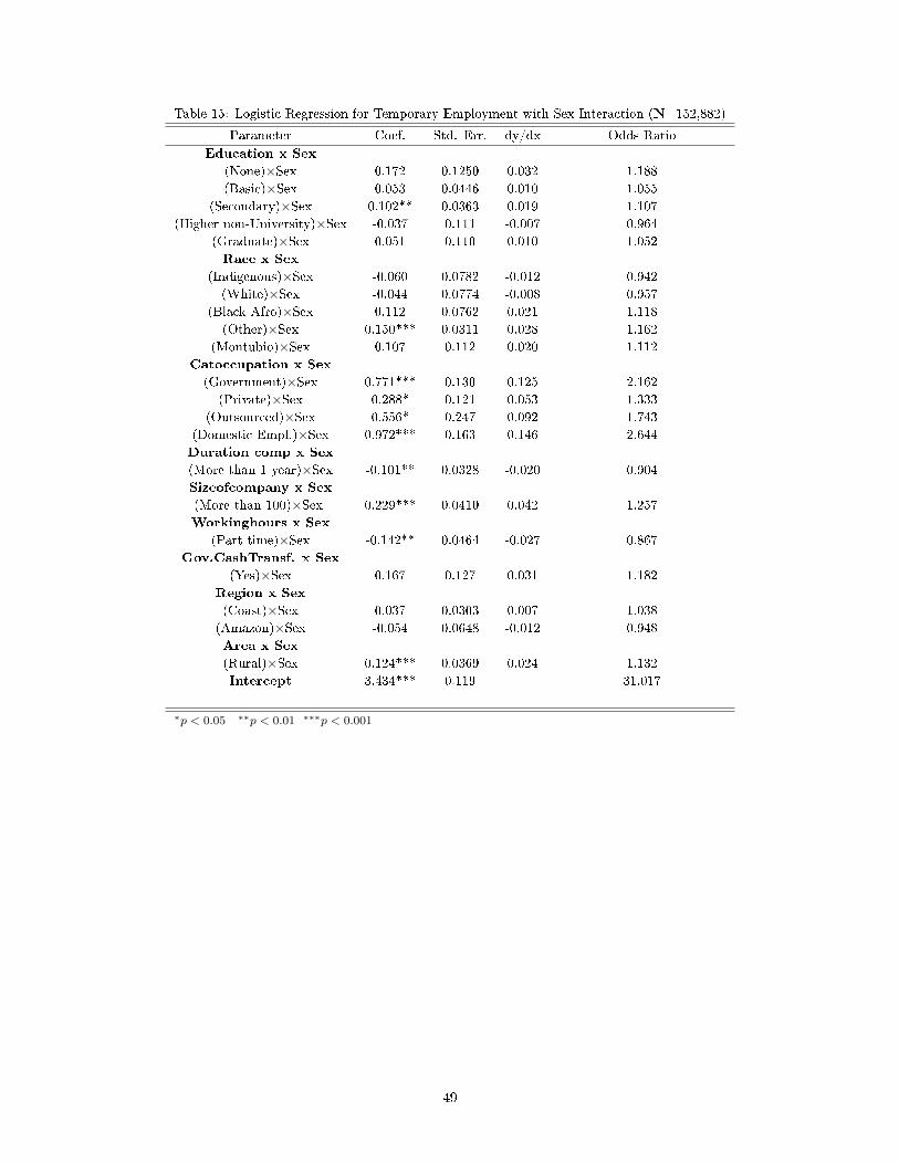
Table 15: Logistic Regression for Temporary Employment with Sex Interaction (N=152,882)

Parameter Coef. Std. Err. dy/dx Odds Ratio

Education x Sex

(None)×Sex 0.172 0.1250 0.032 1.188

(Basic)×Sex 0.053 0.0446 0.010 1.055

(Secondary)×Sex 0.102** 0.0363 0.019 1.107

(Higher non-University)×Sex -0.037 0.111 -0.007 0.964

(Graduate)×Sex 0.051 0.110 0.010 1.052

Race x Sex

(Indigenous)×Sex -0.060 0.0782 -0.012 0.942

(White)×Sex -0.044 0.0774 -0.008 0.957

(Black-Afro)×Sex 0.112 0.0762 0.021 1.118

(Other)×Sex 0.150*** 0.0311 0.028 1.162

(Montubio)×Sex 0.107 0.112 0.020 1.112

Catoccupation x Sex

(Government)×Sex 0.771*** 0.130 0.125 2.162

(Private)×Sex 0.288* 0.121 0.053 1.333

(Outsourced)×Sex 0.556* 0.247 0.092 1.743

(Domestic Empl.)×Sex 0.972*** 0.163 0.146 2.644

Duration comp x Sex

(More than 1 year)×Sex -0.101** 0.0328 -0.020 0.904

Sizeofcompany x Sex

(More than 100)×Sex 0.229*** 0.0410 0.042 1.257

Workinghours x Sex

(Part time)×Sex -0.142** 0.0464 -0.027 0.867

Gov.CashTransf. x Sex

(Yes)×Sex 0.167 0.127 0.031 1.182

Region x Sex

(Coast)×Sex 0.037 0.0303 0.007 1.038

(Amazon)×Sex -0.054 0.0648 -0.012 0.948

Area x Sex

(Rural)×Sex 0.124*** 0.0369 0.024 1.132

Intercept 3.434*** 0.119 31.017

∗p < 0.05 ∗∗p < 0.01 ∗∗∗p < 0.001

49

Table 16: Results of Fairlie Decomposition for Temporary Employment

Number of Obs. = 152,882

Number of Obs. (male) = 101,183

Number of Obs. (female) = 51,669

Pr(Y!=0|G=0) = 0.649

Pr(Y!=0|G=1) = 0.498

Explained gender di�erence = 0.151

Total gender di�erence = 0.082

Parameter Coef. Std. Err. %

Age -0.088*** 0.0079 0.056

Marital Status 0.116*** 0.0104 -0.278

Education -0.202*** 0.0082 2.194

Race -0.025*** 0.0072 0.019

Category Ocupation 1.199*** 0.0128 7.484

Duration in a company -1.338*** 0.0213 -1.650

Size of company -0.523*** 0.0201 0.827

Working hours -1.063*** 0.0340 -1.084

Government Cash Transfer 0.418*** 0.112 -0.387

Region 0.435*** 0.0147 0.480

Area -0.394*** 0.0206 0.546

Intercept 1.759*** 0.0543

∗p < 0.05 ∗∗p < 0.01 ∗∗∗p < 0.001

50

Table 17: Multinomial Logistic Regression for Female* (N=219,777)

Permanent Other Non-Working Out of the labor force

Parameter Coef. Std. Err. RRR Coef. Std. Err. RRR Coef. Std. Err. RRR Coef. Std. Err. RRR

Age [Reference category: 36-45]

15-25 -1.171*** 0.0308 0.310 -0.751*** 0.0257 0.472 0.725*** 0.0440 2.064 0.952*** 0.0235 2.591

26-35 -0.458*** 0.0259 0.633 -0.573*** 0.0224 0.564 0.263*** 0.0420 1.301 -0.224*** 0.0219 0.800

46-55 0.524*** 0.0306 1.688 0.509*** 0.0266 1.663 0.134* 0.0554 1.143 0.582*** 0.0267 1.790

56-65 0.930*** 0.0418 2.534 1.088*** 0.0362 2.969 -0.072 0.0857 0.930 1.582*** 0.0358 4.865

Marital Status [Reference category: Married]

Separated -0.372*** 0.0258 0.690 -0.619*** 0.0217 0.539 -0.204*** 0.0396 0.815 -1.472*** 0.0220 0.230

Single -0.081*** 0.0237 0.922 -0.599*** 0.0208 0.550 -0.087* 0.0341 0.917 -0.698*** 0.0190 0.498

Education [Reference category: University]

None -2.189*** 0.0799 0.112 0.676*** 0.0445 1.965 -0.260** 0.0975 0.771 0.957*** 0.0426 2.604

Basic -1.368*** 0.0275 0.255 0.712*** 0.0239 2.038 -0.153*** 0.0385 0.858 0.776*** 0.0216 2.173

Secondary -0.717*** 0.0228 0.488 0.712*** 0.0226 2.037 0.137*** 0.0331 1.147 0.744*** 0.0201 2.105

Hgher non-University 0.024 0.0717 1.024 0.090 0.0793 1.094 -0.009 0.124 0.991 0.037 0.0733 1.037

Graduate 0.291*** 0.0736 1.338 -0.855*** 0.106 0.425 -0.517** 0.177 0.596 -1.712*** 0.133 0.181

Race [Reference category: Mestizo]

Indigenous -0.016 0.0515 0.985 0.644*** 0.0334 1.904 -0.512*** 0.0737 0.599 -0.398*** 0.0340 0.672

White 0.012 0.0515 1.012 -0.042 0.0447 0.959 0.0983 0.0649 1.103 -0.0012 0.0408 0.999

Black-Afro 0.078 0.0528 1.081 -0.224*** 0.0415 0.800 0.0557 0.0615 1.057 0.234*** 0.0362 1.263

Other -0.073*** 0.0204 0.930 -0.040* 0.0177 0.961 -0.316*** 0.0289 0.729 0.172*** 0.0163 1.187

Montubio 0.082 0.0738 1.086 0.152* 0.0676 1.164 0.101 0.104 1.107 0.345*** 0.0629 1.412

Gov. Cash Transf. [Reference category: No]

Yes -0.885*** 0.0359 0.413 -0.166*** 0.0219 0.847 -0.208*** 0.0429 0.812 0.085*** 0.0209 1.089

Region [Reference category: Sierra-Highlands]

Coast -0.403*** 0.0202 0.668 -0.333*** 0.0171 0.717 0.408*** 0.0282 1.504 0.423*** 0.0157 1.526

Amazon -0.034 0.0424 0.966 -0.097** 0.0351 0.908 -0.094 0.0676 0.911 0.101** 0.0335 1.107

Area [Reference category: Urban]

Rural -0.446*** 0.0253 0.640 0.243*** 0.0183 1.276 -0.276*** 0.0329 0.759 0.079*** 0.0170 1.082

Intercept 1.354*** 0.0295 3.874 0.705*** 0.0282 2.024 -1.421*** 0.0487 0.242 0.371*** 0.0267 1.448

∗p < 0.05 ∗∗p < 0.01 ∗∗∗p < 0.001*Base Category: Temporary Employment

51

Table 18: Multinomial Logistic Regression for Male* (N=208,292)

Permanent Other Non-Working Out of the labor force

Parameter Coef. Std. Err. RRR Coef. Std. Err. RRR Coef. Std. Err. RRR Coef. Std. Err. RRR

Age [Reference category: 36-45]

15-25 -0.678*** 0.0239 0.508 -0.870*** 0.0195 0.419 0.535*** 0.0470 1.707 2.038*** 0.0393 7.673

26-35 -0.216*** 0.0206 0.806 -0.634*** 0.0180 0.530 0.083 0.0485 1.086 -0.101* 0.0452 0.904

46-55 0.225*** 0.0229 1.253 0.442*** 0.0185 1.556 0.315*** 0.0580 1.370 1.011*** 0.0484 2.749

56-65 0.428*** 0.0274 1.535 0.884*** 0.0213 2.420 0.819*** 0.0633 2.267 2.590*** 0.0452 13.326

Marital Status [Reference category: Married]

Separated -0.294*** 0.0295 0.746 -0.113*** 0.0238 0.893 0.560*** 0.0565 1.751 0.533*** 0.0429 1.704

Single -0.382*** 0.0187 0.682 0.011 0.0154 1.011 1.009*** 0.0345 2.742 2.039*** 0.0245 7.686

Education [Reference category: University]

None -2.440*** 0.0628 0.087 -0.827*** 0.0343 0.437 -1.259*** 0.105 0.284 -0.073 0.0443 0.930

Basic -1.664*** 0.0217 0.189 -0.499*** 0.0201 0.607 -1.001*** 0.0387 0.368 -0.846*** 0.0243 0.429

Secondary -0.737*** 0.0199 0.478 -0.139*** 0.0201 0.870 -0.421*** 0.0352 0.656 -0.453*** 0.0234 0.636

Hgher non-University 0.136* 0.0689 1.146 -0.0374 0.0746 0.963 0.069 0.127 1.072 -0.578*** 0.0989 0.561

Graduate 0.486*** 0.0734 1.626 -0.527*** 0.0891 0.590 -0.369* 0.186 0.691 -0.711*** 0.161 0.491

Race [Reference category: Mestizo]

Indigenous -0.123** 0.0388 0.884 0.672*** 0.0251 1.958 -0.010 0.0720 0.990 0.191*** 0.0352 1.210

White 0.0511 0.0402 1.052 0.0301 0.0337 1.031 0.237*** 0.0639 1.267 0.188*** 0.0437 1.207

Black-Afro -0.108** 0.0359 0.898 -0.137*** 0.0257 0.872 -0.015 0.0574 0.985 -0.042 0.0353 0.959

Other 0.007 0.0159 1.007 -0.026 0.0135 0.975 -0.157*** 0.0286 0.854 0.268*** 0.0173 1.308

Montubio 0.126* 0.0562 1.134 0.121* 0.0489 1.128 0.186* 0.0944 1.204 0.357*** 0.0613 1.429

Gov. Cash Transf. [Reference category: No]

Yes -0.804*** 0.0977 0.447 0.232*** 0.0428 1.261 -0.057 0.144 0.945 1.484*** 0.0509 4.412

Region [Reference category: Sierra-Highlands]

Coast -0.683*** 0.0151 0.505 -0.407*** 0.0125 0.666 -0.068* 0.0273 0.934 -0.481*** 0.0160 0.618

Amazon -0.063 0.0331 0.939 0.065* 0.0268 1.068 -0.002 0.0637 0.998 -0.116*** 0.0351 0.891

Area [Reference category: Urban]

Rural -0.798*** 0.0173 0.450 -0.025 0.0128 0.976 -1.090*** 0.0329 0.336 -0.822*** 0.0167 0.440

Intercept 1.221*** 0.0247 3.390 0.640*** 0.0234 1.896 -2.085*** 0.0535 0.124 -2.647*** 0.0454 0.071

∗p < 0.05 ∗∗p < 0.01 ∗∗∗p < 0.001*Base Category: Temporary Employment

52

Table 19: Seemingly Unrelated Bivariate Probit (N=282,878)

Temporary Employment Participate Pr(Temp1=1,Participate=1)

Delta-method

Parameter Coef. Std. Err. Coef. Std. Err. dy/dx Std. Err

Sex [Reference category: Female]

Men 0.043*** 0.0082 0.171*** 0.011 0.008*** 0.001

Age [Reference category: 36-45]

15 -25 0.346*** 0.0113 -0.209*** 0.0161 0.058*** 0.002

26-35 0.158*** 0.0102 -0.100*** 0.0151 0.027*** 0.002

46-55 -0.174*** 0.0120 -0.017 0.0181 -0.029*** 0.002

56-65 -0.292*** 0.0154 -0.057** 0.0218 -0.049*** 0.003

Marital Status [Reference category: Married]

Separated 0.117*** 0.0119 -0.139*** 0.0157 0.019*** 0.002

Single 0.082*** 0.0086 -0.174*** 0.0119 0.013*** 0.001

Education [Reference category: University]

None 0.620*** 0.0281 0.104* 0.0357 0.106*** 0.005

Basic 0.410*** 0.0111 0.102*** 0.0157 0.071*** 0.002

Secondary 0.199*** 0.0095 -0.037* 0.0134 0.035*** 0.002

Higher non-University -0.045 0.0302 -0.014 0.0459 -0.008 0.005

Graduate -0.159*** 0.0297 0.348*** 0.0599 -0.027*** 0.005

Race [Reference category: Mestizo]

Indigenous 0.166*** 0.0192 0.160*** 0.0278 0.028*** 0.003

White -0.020 0.0193 -0.060* 0.0245 -0.004 0.003

Black-Afro -0.032 0.0177 -0.013 0.0224 -0.005 0.003

Other 0.056*** 0.0078 0.112*** 0.0108 0.010*** 0.001

Montubio -0.091 0.0280 -0.022 0.0364 -0.01** 0.005

Category Ocupation [Reference category: Government employee]

Private 0.323*** 0.0104 -0.325*** 0.0185 0.119*** 0.004

Outsourced 0.764*** 0.0438 -0.412*** 0.0612 0.280*** 0.015

Journeyman/Pawn 1.809*** 0.0156 -0.083** 0.0241 0.538*** 0.004

Patrono -7.100 3553.175 0.484*** 0.0461 -0.374*** 0.004

Self Employed -7.265 1269.389 0.267*** 0.0215 -0.374*** 0.004

Unpaid Work -7.444 2008.666 0.664*** 0.0353 -0.374*** 0.004

Domestic Empl. 0.461*** 0.0183 -0.351*** 0.0284 0.171*** 0.007

Gov. Cash Transf. [Reference category: No]

Yes 0.290*** 0.0178 -0.059* 0.0212 0.0474*** 0.003

Region [Reference category: Sierra-Highlands]

Coast 0.258*** 0.0075 -0.132*** 0.0105 0.043*** 0.001

Amazon 0.197*** 0.0165 0.008 0.0245 0.033*** 0.003

Area [Reference category: Urban]

Rural 0.197*** 0.0090 0.354*** 0.0133 0.034*** 0.002

Intercept -0.970*** 0.0138 1.892*** 0.0221

/athrho 2.076*** 0.0429

rho 0.969*** 0.0026

Likelihood-ratio test of rho=0: chi2(1) = 18353.5 Prob > chi2 = 0.0000∗p < 0.05 ∗∗p < 0.01 ∗∗∗p < 0.001

53

Figure 1: Evolution of the Employment, Underemployment and Unemployment

020

4060

%

jul2

007

jan2

009

jul2

010

jan2

012

jul2

013

Underemployment UnemploymentFull Employment

Source: ENEMDU (INEC)

Figure 2: Unemployment Rate for Men and Women

23

45

%

jul2

007

jan2

009

jul2

010

jan2

012

jul2

013

Unemp. Rate Men Unemp. Rate Women

Source: ENEMDU (INEC)

54

Figure 3: Comparison of Unemployment Rates

46

810

12%

2007

2008

2009

2010

2011

2012

2013

Germany BrazilColombia EcuadorUSA Peru

Source: ENEMDU (INEC)

Figure 4: Underemployment Rate for Men and Women

2025

3035

%

01ju

l200

7

01ja

n200

9

01ju

l201

0

01ja

n201

2

01ju

l201

3

Underemp. Men Underemp. Women

Source: ENEMDU (INEC)

55

Figure 5: Economically Active Population (PEA) and Working Age Population

45

67

89

Mill

ions

of P

eopl

e

jul2

007

jan2

009

jul2

010

jan2

012

jul2

013

Economically Active Population Working Age Population

Source: ENEMDU (INEC)

Figure 6: Participation Rate

.54

.56

.58

.6.6

2P

atic

ipat

ion

Rat

e %

jul2

007

jan2

009

jul2

010

jan2

012

jul2

013

Source: ENEMDU (INEC)

56

Figure 7: Participation Rate for Men and Women

4045

5055

60%

jul2

007

jan2

009

jul2

010

jan2

012

jul2

013

Participation Men Participation Women

Source: ENEMDU (INEC)

57

Figure 8: Conceptualization of the Decision process Made by a Person in the Labor Market

(a) Logit/Probit Model

W − T

D

x′β

66

x′β ((

W −NT

(b) Multinomial Probit

W − T

W − F

D

x′γ

>>

x′γ

77

x′γ //

x′γ

((

x′γ

W −O

NW

R

(c) Seemingly Unrelated Bivariate Probit

W W − T

D

x′δ

;;

x′δ ##

⇐⇒ D

z′ψ

::

z′ψ $$

NWA W −NT

D: Decision of the person W-T: Work under temporary contract. W-NT: Work under no temporary contract. W-F: Work under

permanent contract. W-O: Work under other circumstances (Self-employment, etc.). N-W: No working (unemployed). R: Retired or

non-working voluntarily. W: Work. NWA:No working all (unemployed, retired, etc.).

58