an analysis of traditional issue specific and ...summit.sfu.ca/system/files/iritems1/756/gawm 2008,...

An Analysis of Traditional Issue Specific and Macroeconomic Variables on US Commercial Mortgage Backed Securities

by

Stephen Shai Tak Ho

B.Bus.Admin., Simon Fraser University, 2004

PROJECT SUBMITTED IN PARTIAL FULFILLMENT OF THE REQUIREMENTS FOR THE DEGREE OF

MASTER IN BUSINESS ADMINISTRATION

In the Faculty

of Business Administration

Global Asset and Wealth Management Program

Stephen Shai Tak Ho 2008

SIMON FRASER UNIVERSITY

Winter 2008

All rights reserved. This work may not be reproduced in whole or in part, by photocopy of other means, without permission of the authors.

APPROVAL

Name: Stephen S.T. Ho

Degree: Master in Business Administration

Title of Thesis: An Analysis of Traditional Issue Specific and Macroeconomic Variables on Commercial Mortgage Backed Security Spreads

Supervisory Committee:

___________________________________________

Andrey Pavlov Senior Supervisor Associate Professor of Finance

___________________________________________

Andrew Sweeney Second Reader Adjunct Professor of Finance

Date Defended/Approved: ___________________________________________

2

Abstract

This paper examines the effects of traditional issue-specific commercial mortgage

backed securities (CMBS) variables on US CMBS spreads. In addition, a decomposition of

the Conference Board’s US Leading Economic Indicators (LEI) Index will be examined for

each of the ten component’s explanatory power for US CMBS spreads. A qualitative

examination of the history and setting of the US subprime crisis, features of US CMBS, and

an outline of The Conference Board’s US LEI components are provided. This is followed by

an explanation of assumptions and the methodology used for the statistical analysis of the

fourteen variables on CMBS spreads. In addition, the NA REIT Composite Index Dividend

Yield is hypothesized to contribute to the CMBS spreads. A conclusion will contain results

and proposals for an improved model, in contrast to Jadeja and Dorokov (Summer 2008).

This paper closes with a discussion of possible sources of errors and guidance for future

studies.

Keywords:

Commercial Mortgage Backed Securities, CMBS, CMBS spreads, CMBS ratings, percentage

of subordinate debt, loan-to-value, debt-to-service-coverage, LTV, DSC, Leading Economic

Indicators, LEI, US subprime, subprime crisis

Subject Terms:

Commercial Mortgage Backed Securities, CMBS, CMBS spreads, CMBS ratings, Leading

Economic Indicators, LEI

3

Executive Summary

There is a multitude of variables that influence the spreads of Commercial Mortgage

Backed Securities (CMBS). The three traditional issue-specific factors are the CMBS rating

(RAT), the loan-to-value ratio (LTV), and the debt-to-service coverage ratio (DSC). Also, the

percentage of subordinate debt of a CMBS issue (SUB) is widely considered an integral

determinate of spreads. These four traditional issue-specific variables combined with various

macroeconomic influences are hypothesized to significantly affect CMBS spreads.

Empirically, this paper finds CMBS ratings as the dominate driver of CMBS spreads.

While LTV, DSC, and SUB are less sensitive than RAT, these variables are still statistically

significant. This result is consistent with the findings of Jadeja and Dorokov (2008).

Subsequently, the Conference Board’s ten US Leading Economic Indicators (LEI)

components are analyzed for their qualitative relevance and quantitative explanatory value in

determining standardized CMBS spreads. Most of these individual component results are

insignificant; however, as a group of indicators, they are significant and contribute to

improving the explanatory power of the CMBS spreads model. Surprisingly, with the

addition of the NA REIT Composite Index Dividend Yield, this model specification led to a

lower coefficient of determination for standardized CMBS spreads in comparison to the

proposed Ten Factor Hybrid Model.

The statistical test results of Jadeja and Dorokov (2008) are verified and differences

are reconciled. Various model specifications are proposed, analyzed, and discussed in the

context of statistical regressions. A comparison of the results from this paper’s proposed

Ten Factor Hybrid Model for CMBS spreads will demonstrate an improvement in the

coefficient of determination, the F-statistic, and the Durbin Watson statistic over the Three

Factor Model (RAT, SUB, and DSC) proposed by Jadeja and Dorokov (2008). The

conclusion will yield an improved proposed model specification for CMBS pricing (the Ten

Factor Hybrid Model), possible sources of errors, and guidance for future studies.

4

Dedication

I would like to dedicate this paper to two select individuals who have inspired me,

challenged me, supported me, and mentored me in life.

I would like to dedicate this paper to Hui Qing (Cherry) Ou for her faith in my

competence, morality, and adaptability. She continues to drive me to my best – possibly

challenging me a bit too often at times. Cherry’s absurd work ethic has constantly pressured

me to match her efforts, and her dependability has always given me a sense of serenity and

comfort in the most trying of times. I am indebted to her rational decision making abilities

and complementing guidance as I would often be lost without it.

I wish to also dedicate this paper to my father, David T.K. Ho, for his unconditional

love. His support for my decision to take the MBA program is greatly treasured. I wish us

the best for all the years to come. He has been an early inspiration in my life as I aspire to

reach my potential as a financier, business person, and family man during my post-graduate

career.

5

Acknowledgements

I wish to thank the many members of the SFU Faculty who have contributed to my

higher learning (in order of the SFU Global Asset and Wealth Management program time

chronology): Andrey Pavlov for teaching me matrix algebra and Matlab, and also for his

valuable guidance as my Senior Supervisor for this paper, Leyland Pitt for his practical,

insightful, and intricate decomposition of various case studies to build my growing business

acumen, Andrew Sweeney for his practical take on equities analysis and teaching me that

being ‘approximately correct is better than being precisely wrong’ – also for being the

Second Reader of this paper and his practical guidance, Robert Grauer as a friend and

teacher of the plethora of academic theories behind capital markets, Jim McClocklin and

Alex Chin for reconfirming many of my fundamental beliefs in practical relationship

management, and Mark Wexler for opening my eyes to the intriguing world of ethics as well

as providing me a framework for better decision making processes for all of life’s dilemmas.

I would also like to thank my friends Sandeep Jadeja and Dmitry Dorokov for their

time and explanation of their logic and rationale for aspects in their final project. Their

research was a necessary foundation and benchmark to the findings in this paper. In addition,

I wish to thank my good friends in Chris Chen, George Bumstead, Jordan Levine, Warren

Woo, Nick Chang, and Wesley Chan for being my early academic inspirations. Special thanks

to The Chen Family: Uncle Terry, Auntie Kyung, “Hamani,” Lillian, and Chris. Your family

has supported me unconditionally; and I have always found hope and happiness in my times

of despair in the sanctuary that is your home.

And finally, I wish to thank the other three horsemen, Simon Lim, Eric Woo, and

Christian Chia, for their counsel and friendship. There are too many intricacies, complexities,

and enigmas this world has to offer to face individually, and also too much to enjoy alone!

Thank you for all the experiences and takeaways you have each provided me with.

6

Table of Contents

Approval 2

Abstract 3

Executive Summary 4

Dedication 5

Acknowledgements 6

Table of Contents 7

List of Figures 8

List of Tables 18

Qualitative Fundamentals

• History and Setting of the US Subprime and CMBS Crisis 20

• US Commercial Mortgage Back Security Features 24

• US Leading Economic Indicators Introduction 27

Quantitative Modeling and Results

• Generalizations and Assumptions 29

• Input Data Specification Methodology 33

• Regression Models: Report and Reconciliation of Results 36

Conclusion 66

Sources of Errors and Future Studies 68

References List 70

End Notes 72

7

List of Figures

Figure 1: Average US Housing Prices

• note 1998 – 2003 real and nominal appreciation

8

Figure 2: Growth of US and International Structured Finance Issuance

ource: Moody’s Corporation, Investor Presentation (March 2007), available at:

3831/items/236937/MCO%20March%20Long%20

S

http://library.corporate-

ir.net/library/12/123/12

FINAL.pdf

9

Figure 3: Early Warning Signs that CMBS could mirror RMBS performance

Source:

nline.wsj.com/article/SB122703851606838297.html?mod=todays_us_money_and_i

http://o

nvesting&mg=com-wsj

10

http://online.wsj.com/article/SB122703851606838297.html?mod=todays_us_money_and_investing&mg=com-wsj



Figure 4: Dual Time Series Chart: Office versus Multifamily Loan Delinquencies

ource: http://www.reitwrecks.com/2008/08/mortgage-reits-and-cmbs-tail-risk.html

S

11

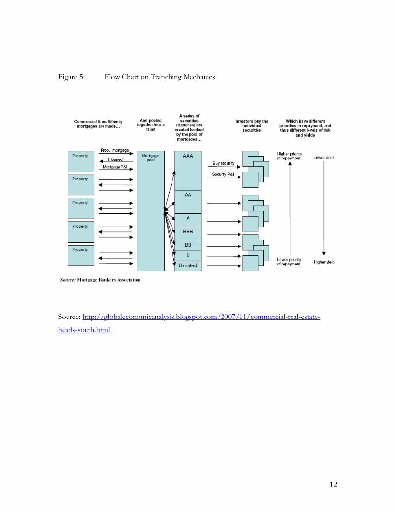
Figure 5: Flow Chart on Tranching Mechanics

ource: http://globaleconomicanalysis.blogspot.com/2007/11/commercial-real-estate-

S

heads-south.html

12

Figure 6: Investors with Capital at Risk in CMBS as of mid-2006

ource: http://globaleconomicanalysis.blogspot.com/2007/11/commercial-real-estate-

S

heads-south.html

13

Figure 7: Time Series Chart mapping the Technology and the later Housing Bubbles

14

Figure 8: BBB CMBS Spreads over 10-year Treasury

ource: http://maoxian.com/archive/cmbs-bbb-spread-now-over-2270-basis-points/

• notice 2006 – 2008 period

S (from

Bloomberg)

15

Figure 9: US CMBS Issuance in $Billions

s

• with Projected 2007 figure

ource: http://www.kennypratt.net/simple/2007/07/key-financing-i.html

S

16

Figure 10: Ten Year CMBS Investment Grade over Swaps Yield

ings

• note increased variance in BBB versus AAA rat

ource: http://www.federalreserve.gov/BoardDocs/HH/2007/july/0707mpr_sec2.htm

S

17

List of Tables

able 1

T : CMBS Unified Rating Valuation Scale

ov (2008) Study

S&P Moody's Fitch Unified Scale

• Identical to the Jadeja and Dorok

Investment Grade

AAA Aaa AAA 19

AA+ Aa1 AA+ 18

AA Aa2 AA 17

AA- Aa3 AA- 16

A+ A1 A+ 15

A A2 A 14

A- A3 A- 13

B B B BB+ aa1 BB+ 12

BBB Baa2 BBB 11

BBB- Baa3 BBB- 10

Non-Investm e ent Grad

BB+ Ba1 BB+ 9

BB Ba2 BB 8

BB- Ba3 BB- 7

B+ B1 B+ 6

B B2 B 5

B- B3 B- 4

CCC+ Caa1 CCC+ 3

CCC Caa2 CCC 2

CCC- Caa3 CCC- 1

18

Table 2: CMBS Rating Valuation Scale with Gap = 10

id Model results

S&P Moody's Fitch Unified Scale

• Used as inputs for the Ten Factor Hybr

Investment Grade

AAA Aaa AAA 29

AA+ Aa1 AA+ 28

AA Aa2 AA 27

AA- Aa3 AA- 26

A+ A1 A+ 25

A A2 A 24

A- A3 A- 23

B B B BB+ aa1 BB+ 22

BBB Baa2 BBB 21

BBB- Baa3 BBB- 20

Non-Investm e ent Grad

BB+ Ba1 BB+ 9

BB Ba2 BB 8

BB- Ba3 BB- 7

B+ B1 B+ 6

B B2 B 5

B- B3 B- 4

CCC+ Caa1 CCC+ 3

CCC Caa2 CCC 2

CCC- Caa3 CCC- 1

19

ualitative Fundamentals

History and Setting of the US Subprime and CMBS Crisis

The year 2008 will be characterized in history by the insolvencies of many iconic US

In March 2000, the Nasdaq Composite Index reached its pinnacle of 5,049; and in

During the time period between December 2001 and November 2004, the US

Due to the resilience of US nominal and real housing prices from 1998, even before

the technology bubble imploded, coupled with historically low interest rates, the confidence

Q

financial institutions such as Bear Stearns, Lehman Brothers, AIG, Countrywide Financial,

and Washington Mutual. However, the reasons for the demise of these US financial pillars

were gradual and compounding, as opposed to sudden and overnight.

October 2002, the Nasdaq Composite Index troughed at 1,116. In about two and a half

years, 77.9% of the Nasdaq Composite market capitalization was erased. Financiers felt a

sense of resentment towards publically traded equities after the technology bubble burst, in

conjunction with a drastically lowered risk appetite. A national portfolio rebalancing towards

asset classes with low systematic risk and lower perceived risk quickly followed.

federal funds target interest rate remained below 2%. This expansive monetary policy

stimulated investment and consumption with lower opportunity costs of capital. However,

insurance companies, and to some extent pension funds, would unlikely be able to cover

their fixed liabilities with low yielding US Treasuries. Thus, in efforts to avoid defaulting on

these liabilities, firms of this nature commenced a search for higher yields for future viability.

It is important to note that as US interest rates were declining, a global appreciation of

housing and other asset prices materialized.i This set the stage for the US commercial and

residential real estate bubbles.

20

in the US real estate asset class increased for investors.ii With this realization along with an

increasing market demand for high yielding securities, investment banks commenced

underwritings of financially engineered products. This led to the proliferation of the

collateralized debt obligation (CDO) securities.

This new demand for CDO securities was unprecedented; but more importantly, it

as an extraordinary event as opposed to a sustainable event. The CDO market itself was

nks and mortgage firms operate in the entrepreneurial worldview

here material abundance is respected, the individual reigns supreme, and the velocity of

decision

housing

market bubble. Expectations of continued rising housing prices, refinancing mortgages at

lower r

w

strong enough to drive demand for underlying mortgages in and of themselves.iii In turn,

these mortgage originations further inflated housing prices. The investment banks and their

structured finance vehicles drove demand for subprime mortgages from the mortgage-

originating lenders. These lenders prospered from each incremental mortgage origination.

Lending standards started to deteriorate as greed and potential for material abundance

prevailed. Although this fact was a major factor for RMBS crisis, this was the primary factor

for the CMBS crisis.

Investment ba

w

-making is valued.iv Compliance becomes an impediment to velocity and that in

itself, hinders a mortgage lending agent from heightened material compensation. Thus, it

should be expected that lending standards fall in this setting, and indeed they did.

Assumptions that should be questioned remained unquestioned in the

ates, and improving credit scores are not rational and sustainable assumptions. Also,

traditional CDOs invested in unique pools of corporate loans and bonds. Systematic risks

are determined by holding various proportions of cyclical and counter-cyclical industries

within the pool. However, the Asset Backed (ABS) CDO securities are dictated by economic

factors on a national level such as interest rates, housing prices, and the labor market; these

systematic risks are non-diversifiable. A critical assumption that ABS CDO securities could

diversify systematic risks like traditional CDO securities was a fallacy. Thus, in the event of a

collapse in housing prices or national economic malaise, the erroneous low beta assumption

of the CDO would have severe consequences as this economic assumption is critical in

21

structuring ABS CDOs. v However, one major assumption differs for the CMBS case:

commercial real estate pricing is cyclical. In hindsight, the CMBS case is even tougher to

digest with this historical fact in mind.

A seemingly more cohesive assumption is that the CDO ratings provided by the big

three rating agencies, S&P, Moody’s, and Fitch, are objective and justified. However,

conflict

A resilient US housing market from 1998 through 2006, unparalleled demand for

high yielding securities in a low interest rate environment, fallacious low systematic risk

CDO a

ime crisis outlined has

fected the less affluent; however, easy credit was a widespread disease. Any loan to any

borrow

s of interests between underwriters and rating agencies plague objectivity and

justification for CDO issue ratings. The rating agencies become a consultant to the

underwriters to achieve desired ratings. The compensation scheme in itself is a conflict of

interest – the rating agencies are compensated by the underwriters. vi This is a typical

example of agent capture.vii Less sophisticated and smaller financial institutions relied more

on ratings provided by the big three credit rating agencies than larger and more sophisticated

financial institutions.viii This factor was more significant for the RMBS crisis as opposed to

the CMBS crisis. Commercial properties are more flexible and easier to transform for other

functions; thus, the CMBS are less susceptible to precipitous price drops than RMBS, status

quo.

ssumptions, and conflicts of interest between rating agencies and underwriters

leading to artificially high CDO issue ratings, together, created the foundation for the

subprime crisis to germinate, fester, and infect the global financial system. The story for the

CMBS market has many parallel similarities with the subprime RMBS crisis: the low interest

rate environment drove demand for higher yielding securities, the conflicts of interest

between rating agencies and the underwriters leading to inflated CMBS ratings, and the

widespread deteriorating lending standards of financial institutions.

On topic with the 2007 US Recession, the current subpr

af

er could be classified as subprime if there is inadequate down-payment or an

exorbitant amount of debt. This is an issue of concern for the commercial real estate market.

Commercial properties of various types enjoyed significant price appreciation since the

22

beginning of this century and delinquencies had fallen to record lows in early 2007. However,

the possible implosion of the CMBS market will be markedly different than the RMBS

precipitous fall: there are no targets of predatory lending and there were no failures by

government regulators. ix The public does not have the less affluent US citizens to

commiserate with for the CMBS scenario as opposed to the RMBS scenario. The corporate

and institutional greed for incremental profit has led to a probably CMBS crisis.

The commercial real estate market crisis will yield less detrimental affects than the

recent housing crisis. It is a smaller market in aggregate and the buildings have a diversified

group o

d per issue,

and the amount of leverage applied have pushed the CMBS market into a state of irrational

exubera

This recession is

largely attributed to the simultaneous collapse of the national housing bubble and the

aggrava

f tenants with various sources of income. In 1995, $15.7 Billion of CMBS were

issued; in the first three quarters of 2007, $196.9 Billion of CMBS were issued.x The market

size for outstanding CMBS issues is $730 Billion. It is important to note that the supply of

commercial real estate was proportionally much less than the residential market and

commercial real estate is easily renovated for a multitude of uses and functions.

Falling lending standards, excessive levels of greed, lofty ratings grante

nce.xi The security underwriting rate was unsustainable, money supply is finite, and

the market was further spurred with fallen lending standards and undeservingly high ratings.

Commercial real estate is cyclical; Wall Street anticipated an inevitable market crash. The

corporations and institutions that have created the CMBS disarray will be held accountable,

slandered, and shown no mercy by the public media and societal factions.

The most recent US recession commenced in December 2007.xii

ting subprime mortgage crisis in 2006. In November 2008, there have been arising

fears of probable widespread distress in the US commercial mortgage back securities (CMBS)

market as indicated by record high risk premiums.xiii With this possible scenario becoming

an economic reality, a study of issue specific and macroeconomic variables influencing

CMBS spreads is pertinent and insightful to the persevering US economic environment.

23

US Commercial Mortgage Back Security Features

mortgage market is comprised of two divisions: the residential mortgage

arket typically includes properties with one to four single family units; and the commercial

to finance a new purchase or refinance an

xisting commercial mortgage obligation. CMBS are non-recourse loans: there is no reliance

ary market demand for ABS CDO securities

as due to tranching. Although tranching does not reduce the absolute degree of risk

edictors of CMBS performance are the CMBS ratings

AT), percentage of subordinate debt (SUB), loan-to-value ratio (LTV), and the debt-to-

The US

m

mortgage market includes income-producing properties such as apartment buildings, office

buildings, industrial warehouse properties, shopping centers, hotels, and health care facilities

for senior housing care and retirement homes.xiv The focus of this paper is strictly within

the confines of the US commercial mortgage market.

Commercial mortgage loans are originated

e

on the capacity of the borrower to repay. Thus, the CMBS holder is only able to depend on

the income-generating property backing the loan for interest and principal repayment. If the

CMBS were to default partially or fully, there will be no recourse to the borrower for the

outstanding unpaid balance; however, the holder of the CMBS has an option to consider

selling the property for repayment proceeds.xv

A significant reason for the extraordin

w

associated with a pool of mortgages, it does distribute risk to various tranches in different

degrees.xvi Each tranch is analyzed by its relevant expected cash flows for its respective

property; thus, each tranch contains unique risks and is priced accordingly. Payouts from the

ABS CDO pool were first allocated to the least risky senior tranches, then the mezzanine

tranches and lastly to the most risky equity tranches. Consistent with each tranch’s risk

characterization, losses were first allocated to equity tranches, then to the mezzanines, and

only lastly to the senior tranches.xvii

The four traditional key pr

(R

24

service coverage ratio (DSC). The CMBS issue rating is provided by the big three credit

rating agencies: Standard and Poor’s, Moody’s, and Fitch. The higher the SUB of a CMBS

issue approximates the issues’ higher sensitivities to riskier tranches and payment default,

status quo. The LTV ratio for CMBS analysis is similar to a price-to-earnings metric for

equity analysis. The numerator (loan) is defined as the outstanding loan amount, and the

denominator (value) is defined as the present value of expected cash flows discounted at a

specified capitalization rate. Thus, the value for the loan figure is the future net operating

income (NOI), rental income subtracting cash operating expenses, discounted by a single

capitalization rate. This is significantly different from a residential mortgage backed security

(RMBS) as RMBS use a market or appraisal figure for value. Therefore, analysts are skeptical

about the forecasting of expected cash flow generation and usage of a single, blunt

capitalization rate for resulting LTV ratios reported. Lastly, the DSC ratio is defined as the

NOI divided by debt service. A ratio greater than one suggests that the income generated

from the property is sufficient to cover debt servicing. Thus, DSC ratio may vary due to

NOI estimates, but to a significantly lesser extent than LTV ratio as discounting is a non-

factor.

In general, CMBS are less exposed to prepayment risk than RMBS. On the loan level,

MBS usually entail prepayment penalty mechanisms in the form of prepayment penalty

cenario analysis with varying assumptions of

efault risk, conditional default rate, timing of defaults, concentration of property geography,

C

points, yield maintenance charges, or specific lockout periods. Defeasance is a popular

mechanism used as funds intended for prepayment are then invested in US Treasury

portfolios. In essence, defeasance mitigates proportional CMBS credit risk exposure since it

is indirectly backed by prepayment funds invested in US Treasuries. There are also

mechanisms on the CMBS structural level acting as call protections. Due to these loan and

structural level CMBS call protections, CMBS trade more similarly to traditional corporate

bonds in contrast to a non-agency RMBS.xviii

Stress tests with Monte Carlo and s

d

and percentage of loss severity are performed to understand sensitivities and risks associated

with CMBS. General risks associated with mortgages include credit risk, liquidity risk,

interest rate risk, and prepayment risk.

25

Comprehension of these general features of the commercial mortgage market and

MBS lead to a better understanding of the composition of ABS CDO securities. A C

portfolio or pool of various heterogeneous CMBS issues, in whole or in part, serves as the

fundamental inputs comprising of CMBS CDO securities.

26

US Leading Economic Indicators Introduction

The Conference Board (CB) is a not-for-profit organization that amalgamates,

alyzes, and disseminates information about economic-based forecasts and market trends

ng is a discussion of each of the LEI components: (1) Manufacturer

verage Work Week (MFG) measures the average work week in hours of manufacturing

employ

an

for over the past 90 years.xix The CB US Leading Economic Indicators (LEI) and its ten

components will be scrutinized in this paper. Although a dichotomous LEI index classified

into periods of expansions for predicting peaks and periods of contractions for predicting

troughs will lead to higher coefficients of determination, the focus will be on the individual

LEI components.

The followi

A

ees in the US. Theoretically, trends in MFG contribute to general economic

forecasting not only on an absolute expansion or contraction level, but on a rate of change

level as well. This statistic is recorded monthly. (2) Initial Jobless Claims (JOB) is a measure

of the number of people filing first-time claims for state unemployment insurance.xx The

higher this number results in a higher unemployment statistic and forebodes lesser economic

activity. This statistic is recorded weekly. (3) Seasonally Unadjusted Durable Goods and

Materials New Orders (ODR_CM) notes the amount of total $US for new orders received

from more than 4,000 manufacturers in more than 85 industries of durable goods in the US.

Growth in ODR_CM has usually occurred in advance of general economic expansion. This

statistic is recorded monthly.xxi (4) Purchasing Manager’s Index (PMI) is an indicator based

on five major indicators: new orders, inventory levels, production, supplier deliveries and the

employment environment. A measurement above 50 represents manufacturing sector

expansion and below 50 signals manufacturer sector contraction.xxii The PMI is measured

on a monthly basis. (5) Seasonally Unadjusted Manufacturing Excluding Defense New

Orders (ODR_XD) is similar to ODR_CM as it is measured in total $US for new orders

received from manufacturers subtracting defense industry related orders. ODR_XD is also

recorded monthly. (6) New Privately Owned Housing Units Authorized by Building Permits

27

in Permit-Issuing Places (BLD) is a proxy measure for housing starts. This metric notes the

number of residential building construction projects that have commenced during a given

month. The more people buying new houses signal economic strength and confidence for

future prospects.xxiii (7) The Standard and Poor’s 500 Index (SPX) is the most commonly

used index to gauge the US large capitalization stock market performance. It includes 500

stocks based on market capitalization, liquidity, and industry grouping among other factors.

The S&P Index is market capitalization weighted and is measured daily.xxiv (8) Inflation

Adjusted M2 (AM2) is a measure of US national money supply. M2 includes M1 plus all

time-related deposits, savings deposits, and non-institutional money-market funds.xxv Money

supply can predict inflationary and deflationary trends and is an important consideration for

adjustments in interest rates. For this study, the CPI (January 1998 = 100, base year) is

factored into the M2 figure in order to adjust for inflation. AM2 is reported on a monthly

basis. (9) The Interest Rate Spread between the 10 Year US Treasury and the Federal Funds

Rate (SPR_10FF) reflects how the market evaluates a longer term economic outlook. If the

spreads widen and report a higher figure, the general expectation is that the economic

outlook is weaker. Higher bond yields also attract investment funds from equity classes. This

figure is recorded daily. And finally, (10) Expectations Portion of the University of

Michigan’s Consumer Sentiment Index (CSI) is a measure of expected consumer sentiment.

This figure is a monthly final output from a formula.xxvi The higher the CSI reading for the

month, the more comfortable consumers are about purchasing, thus, stimulating the

economy. The CSI is measured monthly. Incorporating these ten measured variables

through specified mathematical formulae, the CB produces a composite index with

predictive implications on the US economy.

The methodology for computing the actual inputs into the statistical regression

alysis will be discussed in the ensuing Quantitative Modeling and Results section. an

28

Quantitative Modeling and Results

Generalizations and Assumptions

As with any model that attempts to model reality, this model is a drastic

f the real world. However, the findings and results do contribute to

quares (OLS) model is utilized for the following analysis. OLS is

nly one of many possible methods which a curve can be fitted with data.xxvii This method

simplification o

understanding how CMBS spreads vary with respect to traditional issue-specific and

macroeconomic variables.

The ordinary least s

o

assumes a linear relationship between the dependent variable, the standardized CMBS

spreads, and the independent variables, the traditional issue-specific and macroeconomic

factors. This assumption is quite possibly violated in a realistic context. The “line of best fit”

is that which minimizes that sum of squared deviations of the points of the graph from the

points of the straight line, distances measured vertically.xxviii Therefore, OLS regressions are

very sensitive to outliers. In the spirit of retaining objectivity, no data points were discarded

for all regressions in this paper. OLS assumes non-stochastic independent variables; and in

addition, no exact linear relationship exists between two or more independent variables.xxix

This assumption seems reasonable as inputs are from past recorded data. The error term for

the regression has an expected value of zero. This could be a possible source of error as

many indices are biased upward, even if not for the time periods relevant to this study (for

example, S&P 500 index since inception). The error term of the OLS regression is assumed

to have a constant variance for all observations. Volatility is unlikely constant throughout

time and even doubtfully for the 1998 – 2008 time period of interest. The random variables

are assumed statistically independent in OLS modeling. This is another possible violation

since there are likely positive correlations among independent variables and negative

correlations among other independent variables. In accordance with the Gauss-Markov

29

Theorem, given these assumptions, the estimators of alpha and beta are the most efficient

linear unbiased estimators of alpha and beta in the sense that they have the minimum

variance of all linear unbiased estimators.xxx Finally a more acceptable assumption for OLS

modeling: the error terms are normally distributed in the OLS.

It would be possible to use autoregressive conditional heteroscedasticity (ARCH)

odels and generalized autoregressive conditional heteroscedasticity (GARCH) models for

non-co

ession inputs were from Commercial

ortgage Alert (www.cmalert.com

m

nstant error term modeling. This application for CMBS spread modeling may give

reason to support thy hypothesis that the variance of the error term is not a function of an

independent variable, but instead varies over time depending on past magnitude of errors.

As with inflation, interest rates, and stock market returns, there is often evidence of clusters

of large and small errors.xxxi ARCH and GARCH models could lead to increased efficiency

as Gauss-Markov Theorem may have been violated.

The source data used to compute the regr

M ). From 22,581 possible data points, a subset of 1,589 data

nal and time-series, is used for this study. The source

ata from Commercial Mortgage Alert is a cross-sectional, as opposed to a time-series,

points was used. The discarding of 92.96% of the source data could have severe implications.

This massive amount of discarded data was due to frequently omitted necessary inputs such

as at least one CMBS issue rating from one of the big three credit rating agencies, date of

origination and pricing, originating spread over the benchmark, and the benchmark itself

from the original source data. However, in comparison to the 1,179 observations used in

Jadeja and Dorokov (2008), this study has gathered 34.78% additional data. Thus, embedded

in this study is an assumption that the results from this study’s sample statistical analysis are

consistent with the population’s statistical analysis results. This assumption could possibly be

violated; however, there is no definitive resolution as there is no relative data to compare the

sample against the population results.

A pooled data set, cross-sectio

d

measurement of various data at the CMBS origination date. The dependent variable in

CMBS spreads and the four traditional issue-specific independent variables are classified as

cross-sectional data; whereas, the ten CB LEI components are categorized as time-series data.

30

Thus, there is an implicit assumption that the methodology used to price of CMBS at

origination is consistent throughout the 1998- 2008 period. This assumption is likely violated;

however, time-series data for each CMBS issue would be sparse and intermittent due to the

lack of liquidity and volume of trades on these securities. To the point, the CMBS spread at

origination is assumed to be equivalent to an observed CMBS market spread.

As previously discussed, the two traditional issue-specific CMBS variables in LTV

d DSC contain assumptions of an appropriate capitalization rate and predictions of

ree time periods. Jadeja and

orokov (2008) alleged that a four year cycle is sufficient time to draw conclusions regarding

gging variables from the LEI components. Only the SPX and

PR_10FF are recorded daily; whereas, the other eight variables are recorded either monthly

the following

atistical analysis. None of them by themselves or as a collective group is likely to render

an

incoming cash flows (NOI). The assumptions cannot be analyzed from the source data.

Therefore, this is another possible source of error to consider.

The data set from 1998 – 2008 will be split into th

D

patterns and macroeconomic trends characteristic of the respective period. This explicit time

period separation is also necessary to contrast the results from this study to those of Jadeja

and Dorokov (2008). Results could vary widely depending on the time periods chosen; thus,

careful judgment with economic intuition for separating periods of contraction and

expansion is critical for this study’s results. However, a full time period analysis could

provide some perspective.

There are implicit la

S

or weekly. This will certainly distort the regression line fit the further these variables are

regressed from their recorded date. There is no solution for this issue as daily data does not

exist for these eight variables. Thus, we need to keep in mind that the final coefficient of

determination with any of these eight LEI components is likely understated.

There are many questionable assumptions explicit and implicit in

st

this study’s statistical analysis in absolute futility. OLS modeling assumptions are frequently

violated in practice still yielding significant implications. Possible model misspecification can

have serious impacts; however, being aware at every step of modeling methodology can

31

mitigate undesired errors. A sample size of an absolute 1,589 observations should

approximate results derived from a significantly larger population. The assumption of CMBS

spreads at origination being equivalent to hypothetically observed CMBS market spreads is a

concern. However, there may be no superior procedure available and it is approximately

correct. The exact time period separations, LTV and DSC variance, and frequency of

recorded data measurement concerns are important to recognize; however, these concerns

cannot definitively defeat any conclusions drawn from this statistical study on standardized

CMBS spreads.

32

Input Data Specification Methodology

From Commercial Mortgage Alert (www.cmalert.com), input data was filtered for

ompletion of the following fields: date of origination, LTV, DSC, Country (Only $US

evaluation

riteria for CMBS. The input data included in this study requires at least one rating from any

independent variables, SUB, LTV, and

SC, were not manipulated for the OLS regression inputs. However, a couple of the time-

c

denominated US CMBS issues are included in this study of variables affecting standardized

CMBS spreads), rating (at least one valid rating from any of the big three rating agencies),

percentage of subordinate debt, specified spread in addition to the CMBS benchmark, and

the CMBS benchmark. In order to compute final values for the dependent variable, each

CMBS specific spread is added to the respective CMBS benchmark for each CMBS issue and

tranch. Then this set of absolute CMBS spreads were standardized by subtracting the 3

month US Treasury yield. This was the calculation for the standardized CMBS spread,

dependent variable, for all the subsequent OLS regressions analyses in this paper.

With regards to ratings, S&P, Moody’s, and Fitch all use similar ratings

c

of these big three rating agencies. For cases where a CMBS issue has multiple ratings, the

priority is to use S&P, then Moody’s, then Fitch. The justification for this priority is derived

from the highest to lowest number of outstanding rated CMBS issues. This specification

mirrors that of Jadeja and Dorokov (2008). Ratings are initially scaled with a unified rating

system as specified in Jadeja and Dorokov (2008).xxxii

The remainder of the traditional issue-specific

D

series independent variables in the LEI components required calibration. For inflation

adjusted M2 (AM2), monthly non-adjusted M2 was taken and multiplied by a CPI figure

scaled to a reading of 100 for base month and year, January 1998. Each month in the

inspected time period from 1998 – 2008 is calculated in the same manner. The ten year US

Treasury spread over the Federal Funds Rate was computed by the subtraction of the

respective Federal Funds Target Rate from the daily ten year US Treasury spread for each

33

day for this study’s time horizon, 1998 - 2008. The other eight indicators were sourced and

their raw data was used as inputs for the various OLS regressions.

For the following Regression Model 5, the natural logarithm of the computed

ependent variable CMBS spreads was used. The economic intuition for using this

ion Model 6, there is a gap distinguishing the investment grade CMBS

sues and the non-investment grade CMBS issues. After multiple attempts of trial and error

to narr

gression Model 7 assumes the gap value of 10 incorporated into the ratings

dependent variable. And one step further, Regression Model 7 takes the natural logarithm

d

mathematical function is that there is a supposed non-linear relation between spreads. In

reality, the spread difference between two identical securities with AAA and AA rating is far

smaller than the spread difference between two identical securities with CCC and CC rating,

although both these examples are an absolute one rating separation. Utilizing the natural

logarithm, this transformed CMBS spreads data provides a drastically improved coefficient

of determination.

On Regress

is

ow the possible intervals and find a specific value for this gap, a gap value of 10

appears to be a decent approximation. The purpose of this regression model is to test

whether there is a higher deserved weighting for investment grade versus non-investment

grade CMBS. Pension funds, insurance companies, and other large financial institutional

investors often are restricted to holding only or a very large portion of their assets in

investment grade securities.xxxiii An interesting discovery is that the gap value of 10 on this

scale implies that the difference between investment grade and non-investment grade

securities is approximately 10 grade steps, or more accurately between 5 and 15 grade

steps!xxxiv

Re

in

of this value for each of the outputs. Thus, instead of taking the natural logarithm of the

CMBS spread dependent variable and having each of the independent variables plot against

it, attempting to take the natural logarithm of an independent variable in ratings thought to

have a non-linear relationship to the dependent variable should yield a more precise, fine-

tuning method.

34

Regression Model 8 incorporates Regression Model 7’s assumptions with the

addition of adding the assumption in Regression Model 5, take the natural logarithm of the

ependent CMBS spread variable.

d used directly from the daily source data.

d

Finally, for Regression Model 11, the dividend yield data for the NA REIT

Composite Index was unchanged an

This explanation to the input data specification methodology has set the foundation

for the succeeding statistical regression analysis discussion.

35

Regression Models: Report and Reconciliation of Results

The sourc ith the additions

f the macroeconomic LEI components data are jointly tested as possible determinants of

MBS spreads using OLS regression modeling. There are a number of hypotheses to

a set and the more extensive 1,589

bservation data set.

SPRi = α + β1RATi + β2SUBi + β3DSCi + εi

SPR = Standardized spr

AT = Rating issued for CMBS at date of origin

UB = Percentage of subordinate debt for CMBS issue at origination

r CMBS issue at origination

e of the originating CMBS structures from 1998 – 2008 w

o

C

consider for this study: (1) a natural hypothesis is that the key driver of CMBS spreads will

be the credit rating agency issued CMBS rating; (2) traditional issue-specific variables in SUB,

LTV, and DSC are significant, but their variation should affect the CMBS spreads to a lesser

extent than ratings; (3) there should be some explanatory value in some of the ten

components of US LEI. As a group of variables, they should be significant and increase the

explanatory power of the CMBS spreads regression model, even if some of these

macroeconomic variables are insignificant by themselves; and (4) the dividend yield of the

NA REIT Composite Index should increase the explanatory power of a specified model

used to explain the variances of standardized CMBS spreads. The following Regression

Models, 1 to 11, take the full data set from 1998 – 2008.

Beginning with the Jadeja and Dorokov (JD) (2008) Three-Factor regression model,

a comparison is made between their 1,179 observation dat

o

ead on CMBS

R

S

DSC = Debt-to-service coverage ratio fo

36

Table A: Beta and T-stat results from JD (2008) 3-factor model

β i /(T-stat)

Period # of Obs. α RAT SUB DSC

1998 – 2002 469 4.94 -0.20 0.00 -0.15

(35.43) (-1 2) (-4.58) 9.08) (0.9

2003 - 2006 2.96 529 -0.16 0.01 0.06

(22.20) (-17.91) (4.53) (4.23)

2007 - 2008 181 2.91 -0.12 0.02 0.01

(4.94) (-3.88) (2.47) (0.15)

1998 - 2008 1179 4.48 -0.21 0.02 -0.15

(41.86) (-27.39) (-9.11) (9.40)

Table B: Beta and T-stat results from Expanded Data Set with JD (2008) three-factor

model specification

β i /(T-stat)

Period # of Obs. α Rating SUB DSC

1998 - 2002 990 487.97 -20.24 -0.74 -10.41

(35.27) (-2 75) (-2.70) 0.52) (-2.

2003 - 2006 555.57 412 -33.05 2.98 7.79

(22.92) (-17.99) (6.20) (3.01)

2007 - 2008 187 415.21 -17.12 0.65 -9.28

(13.74) (-8.71) (1.42) (-1.59)

1998 – 2008 1589 482.00 -22.43 0.31 -3.20

(1.46) (-1.71) (45.60) (-28.12)

37

Due to the difference in scaling where JD (2008) used spreads in percentage terms,

this regressio used spreads measured in basis points; thus, there is a factor of 100 to adjust

ons, this data set has more than twice the

e

2008 periods. These differences disappear

d significant for the RAT beta.

ant. A natural prediction would be for the

n

for. In contrasting the number of observati

observations for the 1998 – 2002 period than that of JD (2008), 990 versus 469. However,

for the period of 2003 – 2006, the JD (2008) data set is larger, 529 versus 412 observations.

The difference for the 2007 – 2008 period is negligible.

As expected, the alpha terms for both sets of data are positive and significant for all

time periods and for the full data set. However, there are noticeable absolute valu

differences for the 2003 – 2006 and the 2007 –

when comparing both data sets’ full time horizon from 1998 – 2008.

Also hypothesized, the beta for RAT is negative as the higher the rating, the lesser

the CMBS spread should be due to lower risks, status quo. Both data sets for all time period

variations are negative an

However, the results for the SUB and DSC between both data sets are different. JD

(2008) found that SUB and DSC are both significant; whereas, the extended data set

concluded that SUB and DSC are both insignific

SUB beta to be positive as the higher proportion of subordinate debt should increase the

risk in the CMBS security; and thus, it should lead to a higher compensating spread for

investors. For the full 1998 – 2008 time horizon, both data sets have positive SUB betas.

However, for each of the three separate time periods, the results between both data sets are

mixed for significance and sign. Similar to SUB, the null hypothesis is a negative DSC beta.

The higher the DSC is, the less likely the CMBS issue is to default due to increased

compensating cash flows from the property to service debt. In the full 1998 – 2008 time

horizon, the DSC beta sign was confirmed negative for both data sets; however, again, there

are discrepancies for significance and sign when comparing the three separate time periods.

38

Table C: R2, F-stat, Critical F-stat, and DW-test from JD (2008) 3-factor model:

Period R2 F-stat Critical F-Test DW-stat

1998 – 2002 0.56 196.68 8.53 0.73

2003 – 2006 0.51 184.14 8.53 0.76

2007 – 2008 0.09 6.01 8.54 0.25

Full Data 0.46 328.54 8.53 0.49

Table D: Comparable R2, F-stat, Critical F-stat, and DW results from the

Expanded Data Set:

-test

Period R2 F-stat Critical F-Test DW-stat

1998 – 2002 0.45 271.44 8.53 0.82

2003 – 2006 0.52 149.19 8.53 0.91

2007 – 2008 0.40 40.12 8.54 0.65

Full Data 0.44 418.12 8.53 0.77

From Table C and Table D, the coefficient of determination for 2007 – 2008 is

ramatically different with a better result yielded from the expanded data set, R2 equal 0.40

ectively. However, the expanded data set results in a slightly poorer fit with

d

versus 0.09, resp

the 1998 – 2002 data and also the full 1998 – 2002 time horizon (a difference of 0.11 and

0.02, respectively). F-stat were significant for all time periods in the expanded data set in

contrasts to JD (2008) having an insignificant F-stat for the 2007 – 2008 time period. This

39

difference alone supports the added value of the expanded data set. Another premise to

support the expanded data set is the higher DW-test statistics for each of the three time

periods in conjunction with the full time horizon. Although, all computed DW-test statistics

indicate the presence of positive correlation, the expanded data set yields higher DW-test

statistics indicating a lesser likelihood for positive serial correlation.

With conflicting results for the three separated time periods, a more general focus is

taken for the following Regression Models 1 to 11. The results appear more consistent and

etter with a larger sample observation size and longer time horizon. Also, the choice of the

ariables

R

SPR = Standardize

RAT = Rating issued for CMBS at date of origin

SUB = Percentage of subordinate debt for CMBS issue at origination

ue at origination

issue at origination

b

specific separation of time periods requires additional scrutiny as it should have very

significant effects on the regression time period specific results.

Regression Model 1: Traditional Issues-Specific Independent V

SP i = α + β1RATi + β2SUBi + β3LTVi+ β4DSCi + εi

d spread on CMBS

LTV = Loan-to-value ratio for CMBS iss

DSC = Debt-to-service coverage ratio for CMBS

40

Table E: Beta and T-stat results from Regression Model 1:

β i /(T-stat)

# of Obs. α RAT SUB LTV DSC

1589 453.93 -22.39 0.37 -0.78 0.28

(19.03) (-28.05) (1.33) (1.31) (-0.30)

Table F: Regres n Mod ul st c t, -stat):

R2 F-stat Critical F-stat DW-stat

sio el 1 res ts (R2, F- at, criti al F-sta and DW

0.44 314.16 5.63 0.78

This model specification is similar to the JD (2008) three factor model with the

dition of LTV. The sign for each beta value is consistent for each with the pre-regression

alyses theoretical hypotheses. However, only the ratings variable and the alpha are

statistic

ad

an

ally significant. The coefficient of determination at 0.44 for this model is still

marginally lower than the JD (2008) benchmark at 0.46. However, the DW-statistic is higher

and indicates less presence of serial correlation.

41

Regression Model 2: Macroeconomic US LEI Component Independent Variables

Di

+ β7SPXi + β8AM2i + β9SPR_10FFi + β10CSIi + εi

SPR = Standardized

FG = Manufacturer average work week

B = Initial jobless claims

ble goods and materials new orders

justed manufacturing excluding defense new orders

x

ersity of Michigan’s Consumer Sentiment Index

SPRi = α + β1MFGi + β2JOBi + β3ODR_CMi+ β4PMIi + β5ODR_XDi + β6BL

spread on CMBS

M

JO

ODR_CM = Seasonally unadjusted dura

PMI = Purchasing Manager’s Index

ODR_XD = Seasonally unad

BLD = New privately owned housing units authorized by building permits

SPX = Standard and Poor’s 500 Inde

AM2 = Inflation Adjusted M2

SPR_ 10FF = 10 year US Treasury and Federal Funds Rate Spread

CSI = Expectations portion of the Univ

42

Table G: Beta and T-stat results from Regression Model 2:

βi /(T-stat)

# o ORD_XD f Obs. α MFG JOB ORD_CM PMI

1589 2292.7 -39.6 0 0 0.7 0

(3.39) (-2.47) (-4.8 ) (0.49) (-3.68) 1) (2.65

βi / stat) (T-

BLD SPX AM2 SPR_10FF CSI

-0.6 0.1 0 -0.7 -2.4

(-3.46) (4.86) (-0.04) (-0.13) (-3.58)

Table H: Regre od su


ssion M el 2 re lts (R2, F-stat, critical F-stat, and DW-stat):

0.06 10.19 2.54 1.07

Due to the disparity of data recording uency be n each of the ten US LEI

ariables, a depressed coefficient of determination was expected. However, the results do

ate that the combination of all ten US LEI significantly contribute to the variation in

freq twee

v

st

standardized CMBS spreads, F-stat of 10.19 is greater than the Critical F-stat of 2.54. This

model also exhibits lesser positive correlation than the JD (2008) benchmark, 1.07 versus

0.48 DW-stat, respectively. The JOB, ORD_CM, PMI, ODR_XD, and AM2 beta variables

round to zero and thus, it is not possible to conclude any of their beta signs to confirm or

refute the null hypotheses. The theoretical predictions for LEI beta signs are positive for

JOB and SPR_10FF and negative for the other eight variables: MFG, ORD_CM, PMI,

ODR_XD, BLD, SPX, AM2, and CSI. The results from Regression Model 2 appear weak as

the resulting beta signs appear mixed, but seven of the individual betas have statistically

43

significant T-stats. With seven individual statistically significant T-stats of the ten and a

significant F-statistic for the group of ten US LEI components, there is merit for further

analysis in order to possibly specify a model better than JD (2008) incorporating the CB LEI

indicators.

Regression Model 3: Traditional and Macroeconomic Independent Variables

+ R_CMi +

β8PMIi + β9ODR_XDi + β10BLDi + β11SPXi

+ β12AM2i + β 13SPR_10FFi + β 14CSIi + εi

SPR = Standardized spre



ssue at origination


ders


x


SPRi = α + β1RATi β2SUBi + β3LTVi+ β4DSCi + β5MFGi + β6JOBi + β7OD

ad on CMBS

R

S

LTV = Loan-to-value ratio for CMBS i


MFG = Manufacturer average work week

JOB = Initial jobless claims

ODR_CM = Seasonally unadjusted durable goods and materials new or

PMI – Purchasing Manager’s Index







44

Table I: Beta and T-stats from Regression Model 3:

βi /(T-stat)


1589 1925 -21.4 0 0.5 4.4

(3.85) (-27.01) (1.68) (1.37) (-0.14)

-stat) βi /(T

MFG JOB ORD_CM PMI ORD_XD

-24.2 0 0 0.3 0

(-2.04) (-5.81) (0.24) (-4.51) (3.03)

βi /( t) T-sta


-0.6 0.1 0 -1 -2.6

(-4.30) (5.98) (0.40) (-0.23) (-5.20)

Table J: Regressi e u


on Mod l 3 res lts (R2, F-stat, critical F-stat, and DW-stat):

0.49 107.57 2.13 0.84

Regression Model 3 results for the traditional issue-specific variables are consistent

ith Regression Model 1. Only RAT is significant while SUB, LTV, and DSC were

atistically insignificant at the 5% level. Also, Regression Model 2 results are similar to

w

st

Regression Model 3; only PMI, AM2, and SPR_10FF are insignificant, while signs vary for

US LEI components. However, with the fourteen-variable regression, the coefficient of

determination is better than the benchmark of 0.46 and yields a DW-statistic that is again

better than the JD (2008) benchmark indicating lesser evidence of serial correlation.

45

Although Regression Model 3 yield better results than the JD (2008) three-factor model, the

additional eleven factors added only incremental explanatory value for standardized CMBS

spread variation. The model specifications that follow will include economically and

statistically intuitive transformations in attempt to yield a more reality conforming model

than this cumbersome fourteen-variable model.

Regression Model 4: Statistically Significant Traditional and Macroeconomic Independent

Variables

SPRi = α + β 2MFGi + β3JOBi + β4ODR_CMi + β5ODR_XDi

+ β6BLDi + β7SPXi + β8CSIi + εi

SPR = Standardized spread o


FG = Manufacturer average work week

nd materials new orders

cturing excluding defense new orders

housing units authorized by building permits

Index

1RATi + β

n CMBS

R

M


ODR_CM = Seasonally unadjusted durable goods a

ODR_XD = Seasonally unadjusted manufa

BLD = New privately owned

SPX = Standard and Poor’s 500 Index

CSI = Expectations portion of the University of Michigan’s Consumer Sentiment

46

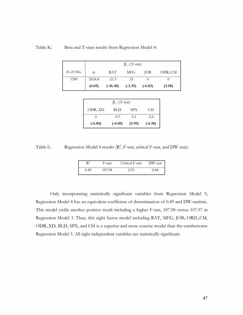
Table K: Beta and T-stats results from Regression Model 4:

βi /(T-stat)

# of Obs. α RAT MFG JOB ODR_CM

1589 2024.8 -21.5 -25 0 0

(6.69) (-36.30) (3.58) (-3.35) (-6.03)

staβi /(T- t)

O D DR_X BLD SPX CSI

0 -0.5 0.1 -2.6

(-6.84) (-4.60) .95) (-6.10) (5

Table L: Regression M esul -s tic t, and DW-stat):


odel 4 r ts (R2, F tat, cri al F-sta

0.49 187.98 2.93 0.84

Only incorporating statistically significant variables from Regression Model 3,

egression Model 4 has an equivalent coefficient of determination of 0.49 and DW-statistic.

his model yields another positive result including a higher F-stat, 187.98 versus 107.57 in

R

T

Regression Model 3. Thus, this eight factor model including RAT, MFG, JOB, ORD_CM,

ODR_XD, BLD, SPX, and CSI is a superior and more concise model than the cumbersome

Regression Model 3. All eight independent variables are statistically significant.

47

Regression Model 5: ln(SPRi) w/ Traditional and Macroeconomic Independent Variables

+ β8PMIi + β9ODR_XDi + β10BLDi + β11SPXi

+ β12AM2i + β13SPR_10FFi + β14CSIi + εi


RAT = Rating issued for CMBS at date of origin

SUB = Percentage of subordinate debt for CMBS issue at origination

ssue at origination


ders


x


ln(SPRi) = α + β1RATi + β2SUBi + β3LTVi+ β4DSCi + β5MFGi + β6JOBi + β7ODR_CMi

ad on CMBS













48

Table M: Beta and T-stats from Regression Model 5:

βi /(T-stat)


1589 8.04 -0.13 -0.01 0.01 0.06

(2.65) (-27.27) (4.10) (3.05) (-4.61)

T-stat) βi /(


0.09 0.00 0.00 -0.01 0.00

(1.20) (-6.40) (-1.20) (-6.11) (2.59)

-stat) βi /(T

BLD SPX AM2 SP R_10FF CSI

0.00 0.00 0.00 0.00 -0.03

(-5.36) (8.99) (0.36) (-0.18) (-8.48)

Table N: Regres d su , F-stat, critical F-stat, and DW-stat):


sion Mo el 5 re lts (R2

0.57 148.65 2.13 0.49

Regression Model 5 is a slight digression from Regression Model 4. There is

conomic intuition that standardized CMBS spreads do not have a linear relationship to

any traditional issue-specific and macroeconomic variables. This model is a generalized test

e

m

to uncover this premise. The results are interesting: all four traditional variables in RAT,

SUB, LTV, and DSC are statistically significant; however, SUB and DSC have theoretically

contradicting signs (although the absolute beta value is miniscule at -0.01 and 0.06). The

previously insignificant US LEI variables in PMI, AM2, and SPR_10FF are still insignificant;

49

however, now MFG has also become insignificant. It is important to note that the already

small absolute value of beta coefficients observed for Regression Model 3 is further

minimized in Regression Model 5. However, it is tough to argue against the statistically

significant and much higher coefficient of determination of 0.57 versus 0.49; however, this is

at the expense of additional presence of serial correlation with a 0.49 DW-stat, in contrast to

the 0.84 DW-statistic for Regression Model 3. Note that 0.49 DW-statistic is the reading for

the JD (2008) three-factor model. From this model specification, there is probability that

natural logarithm modeling could lead to improved model specification, thus, confirming

economic rationale.

50

Regression Model 6: Traditional (incorporating an investment grade ratings gap of ten)

and Macroeconomic Independent Variables

SPRi = α + β1[RATi,( i+ β4DSCi + β5MFGi +

β6JOBi + β7ODR_CMi + β8PMIi + β9ODR_XDi + β10BLDi + β11SPXi

+ β12AM2i + β13SPR_10FFi + β 14CSIi + εi




ssue at origination


ders


x


+10 if investment grade)] + β2SUBi + β3LTV

ad on CMBS

R

S













51

Table O: Beta and T-stats from Regression Model 6:

βi /(T-stat)


1589 1872.1 -18.3 -0.2 0.6 5.9

(4.02) (-32.73) (2.19) (1.95) (-1.01)

-stat) βi /(T

MFG M D JOB ORD_C PMI ORD_X

-19.5 0 0 0.7 0

(-1.76) (-6.30) (4.16) (0.70) (-6.08)

βi stat) /(T-


-0.5 0.1 0 -4.1 -3

(-4.06) (6.92) (1.03) (-1.08) (-6.36)

Table P: Regres d su vario ng “g es:

(R2, F-stat, critical F-stat, and DW-stat):

sion Mo el 6 re lts for us Rati ap” valu


Gap = 1 0.50 113.63 2.13 0.84

Gap = 5 0.54 131.93 2.13 0.85

Gap = 10 0.56 140.20 2.13 0.90

Gap = 15 0.55 138.31 2.13 0.95

Gap = 20 0.54 132.82 2.13 0.98

For Regression Model 6, the basis ression el 3 wit transformation of

e RAT data to include a hypothetical “gap” between investment grade and non-investment

sues. In the JD (2008) study, JD utilized a unified and linear scale for

is Reg Mod h the

th

grade CMBS is

52

assigning and quantifying CMBS ratings. However, in the investment world reality with

established financial institutions, there are many constraints that often preclude non-

investment grade securities. Thus, there is a “gap” in reality between these divisions.xxxv

The primary issue is to test if this theory of a ratings “gap” between investment

grade and non-investment grade securities is confirmed by the regression models. The

condary issue is to approximate a decent “gap” value for subsequent regression models.

PX, and CSI; however, the specific significant variables in this model are

ot exactly identical to Regression Model 3. LTV was statistically insignificant in Regression

se

From Table P, it is evident that the “gap” in fact does exist according to the result’s

implications. Each of the coefficients of determination for the various “gap” model values

yields a statistically significant and higher R2 than without the “gap” (Regression Model 3

yielded a 0.49 R2).

For the beta coefficients, eight of them were significant: RAT, LTV, JOB, ODR_CM,

ODR_XD, BLD, S

n

Model 3, while MFG was statistically significant. A “gap” value of 10 yielded the highest R2

of 0.56 and is, therefore, a better predictor for standardized CMBS spreads than Regression

Model 4 at 0.49.

53

egression Model 7: Traditional (incorporating an investment grade ratings gap of ten,

then taking the natural logarithm of the computed value) and

Macroeconomic Independent Variables

SPRi = α + β1ln[RATi, 3LTVi+ β4DSCi + β5MFGi +

β6JOBi + β7ODR_CMi + β8PMIi + β9ODR_XDi + β10BLDi + β11SPXi





ssue at origination


ders


x


R

(+10 if investment grade)] + β2SUBi + β

ad on CMBS

R

S













54

Table Q: Beta and T-stats from Regression Model 7:

βi /(T-stat)


1589 2304.8 -328.9 -0.8 0.7 6.6

(5.22) (-37.05) (2.60) (2.33) (-5.01)

stat) βi /(T-

MFG M D JOB ORD_C PMI ORD_X

-14.3 0 0 0.9 0

(-1.36) (-6.46) (5.16) (0.90) (-7.33)

Table R: Regres d su , F-stat, critical F-stat, and DW-stat):


sion Mo el 7 re lts (R2

0.60 169.01 2.13 0.96

Regression Model 7 is an evolution of Re n Model 6. As previously discussed,

ere is economic and statistic reasons to assume non-linearity relationships between select

ariables. This non-linearity is incorporated by natural logarithmic modeling. Regression

βi stat) /(T-


-0.5 0.1 0 -5.2 -3.3

(-3.92) (7.64) (1.18) (-1.44) (-7.52)

gressio

th

v

Model 5 yielded stellar relative results with natural logarithmic modeling of the standardized

CMBS spread; however, it was too general and a logical hypothesis would be to evaluate

each variable for a possible non-linear relationship with SPR. Thus, Regression Model 7

55

factors in a ratings “gap” value of ten for investment grade CMBS issues and transforms the

data with a natural logarithm function.

The results for this model specification are encouraging. This iteration has ten

atistically significant of the fourteen possible independent variables. This is the highest st

number of statistically significant independent variables for the SPR modeling sequence.

Only MFG, PMI, AM2, and SPR_10FF are insignificant variables. Furthermore, the four

traditional issue-specific variables in RAT, SUB, LTV, and DSC are each statistically

significant. The 0.60 R2 is the highest in all iterations thus far along with a high F-statistic of

169.01 and substantially better than the JD (2008) benchmark DW-statistic with 0.96. The

fine-tuning and transformation of the RAT variable led to improved results.

56

Regression Model 8: ln(SPRi) and Traditional (incorporating an investment grade ratings

gap of ten, then taking the natural logarithm of the computed value)

ln(SPRi) = α + β1ln[RATi,(+10 if investment grade)] + β2SUBi + β3LTVi+ β4DSCi +

β5MFGi + β6JOBi + β7ODR_CMi + β8PMIi + β9ODR_XDi + β10BLDi + β11SPXi

PR = Standardized spread on CMBS


for CMBS issue at origination

ination

goods and materials new orders

Index

g units authorized by building permits

Federal Funds Rate Spread

the University of Michigan’s Consumer Sentiment Index

and Macroeconomic Independent Variables


S

R

SUB = Percentage of subordinate debt

LTV = Loan-to-value ratio for CMBS issue at orig

DSC = Debt-to-service coverage ratio for CMBS issue at origination



ODR_CM = Seasonally unadjusted durable

PMI = Purchasing Manager’s

ODR_XD = Seasonally unadjusted manufacturing excluding defense new orders

BLD = New privately owned housin



SPR_ 10FF = 10 year US Treasury and

CSI = Expectations portion of

57

Table S: Beta and T-stats from Regression Model 8:

βi /(T-stat)


1589 9.82 -1.42 0.01 0.07 -0.02

(3.05) (-21.89) (-13.73) (4.10) (3.17)

-staβi /(T t)


0.12 0.00 -0.01 0.00 0.00

(1.63) (-6.02) (3.86) (-0.97) (-7.26)

stat) βi /(T-


0.00 0.00 -0.02 -0.03 0.00

(-4.88) (9.04) (-9.07) (0.32) (-0.65)

able T: Regression Model 8 results (R2, F-stat, critical F-stat, and DW-stat): T


0.51 118.86 2.13 0.58

Not predictably, Regression Model 8 results are inferior to Regression Model 7

sults. From improved regression results yielded by Regression Model 5 for ln(SPRi) and

re

Regression Model 7 for taking the natural logarithm of a “gap” adjusted RAT data, the

natural hypothesis would be that a combination of these model specifications would lead to

improved results again; however, this was not the case. The coefficient of determination

dropped 0.09 or by 15%, the DW-statistic worsened significantly to 0.38, and the F-stat

dropped. As likely as there are non-linear relationships, there are possible linear relationships.

58

By taking the natural logarithm of SPR and also of the RAT approximately cancels out the

intention of non-linearity as yielded by Regression Model 7. Thus, Regression Model 7 with

its ten statistically significant independent variables is the final model specification for

modeling SP

Regression Model 9: Statistically Significant Traditional (incorporating an investment grade

ratings gap of ten, then taking the natural logarithm of the computed

SPRi = α + β1ln[RATi,(+10 if investment grade)] + β2SUBi + β3LTVi+ β4DSCi +

β5JOBi + β6ODR_CMi + β7ODR_XDi + β8BLDi + β9SPXi + β10CSIi + εi




ination

ders


iment Index

value) and Macroeconomic Independent Variables

S

R









CSI = Expectations portion of the University of Michigan’s Consumer Sent

59

Table U: Beta and T-stats from Regression Model 9:

βi /(T-stat)


1589 1777.6 -328.2 0.7 7.7 -0.9

(27.20) (-37.20) (-5.27) (2.70) (2.89)

t) βi /(T-sta

JOB ORD_CM ORD_XD BLD SPX CSI

0 0 -0.4 0.1 -3.6 0

(-6.32) (5.31) ( (-10.44) (-10.03) (-4.13) 8.29)

able V: Regression Model 9 results (R2, F-stat, critical F-stat, and DW-stat): T


0.60 235.67 2.54 0.96

Regression Model 9 is the final model specification for the analysis of SPR. With ten

atistically significant independent variables, all four traditional issue-specific variables and

st

six of the ten US LEI components as variables, this model has achieved an R2 of 0.60, and

high F-statistics and DW-statistics in contrast to the three-factor model from JD (2008).

Regression Model 9 is the Ten Factor Hybrid Model specification.

60

Regression Model 10: Statistically Significant Traditional (without RAT) and

Macroeconomic Independent Variables

SPRi = α + β1SUBi + β2LTVi+ β3DSCi + β4JOBi + β5ODR_CMi

+ β6ODR_XDi + β7BLDi + β8SPXi + β9CSIi + εi



ssue at origination

ders


iment Index

S

S









61

Table W: Beta and T-stats from Regression Model 10:

βi /T-stat

# of Obs. α SUB LTV DSC

1589 901.51 -3 1.91 .85 0.30

(-10.80) (-20.11) (-0.81) (0.52)

βi /T-stat

JOB ORD_CM ORD_XD BLD SPX CSI

-0.00 0.00 -0.00 -0.60 0.13 -3.39

( ( (-7.28) -5.33) (5.64) (-8.94) (-4.71) 5.50)

able X: Regression Model 10 results (R2, F-stat, critical F-stat, and DW-stat): T

R2 F-stat critical F-stat DW-stat

0.25 51.85 2.54 0.91

The specification this regression formula and its analysis focus on the importance of

le as a determinant for standardized spreads on the CMBS issues. From

the RAT variab

Regression Model 10, the fall of 0.35 in the coefficient of determination is more significant

than hypothesized leading to a final figure of 0.25 for Regression Model 10. This is a 58%

drop in the explanatory power of the model omitting the RAT variable. Although there is no

quantification of the degree of importance of the RAT, it is surprising that its effects

outweigh the explanatory power of the other nine variables by 40%! The F-statistic also falls

dramatically to 51.85 from a figure of 235.67 in Regression Model 9. These results have

fascinating real world implications. There is evidence to support the fact that investment

managers depend disproportionately high on the ratings of an issue in contrast to other

considered variables. This fact alone supports the higher than expected amount of

62

devastation that the ratings agencies have on the CMBS markets, status quo. The conflicts of

interest that plague the underwriting and ratings issued from the perspective of S&P,

Moody’s, and Fitch were understated. This is derived from the analysis of the importance of

the RAT variable.

Regression Model 11: Statistically Significant Traditional (incorporating an investment grade

ratings gap of ten, then taking the natural logarithm of the computed

SPRi = α + β1ln[RATi,(+10 if investment grade)] + β2SUBi + β3LTVi+ β4DSCi +

β5JOBi + β6ODR_CMi + β7ODR_XDi + β8BLDi




ination

ders


iment Index

vidend yield

value) and Macroeconomic Independent Variables and US REIT

Composite Index dividend yield

+ β9SPXi + β10CSIi + β11REITi + εi

S

R










REIT = NA REIT Composite Index di

63

Table Y: Beta and T-stats from Regression Model 11:

tat

βi /T-stat


1589 8.53 -0.13 0.01 0.06 -0.01

(-16.59) (-28.33) ( -4.47) (5.52) (3.12)

βi /T-s

JOB ORD_CM ORD_XD BLD SPX CSI REIT

0.00 0.00 0.00 01 0.00 -0.02 0.17 -0.

(-7.04) (-3.19) (-8.95) (3.05) (-8.06) (0.21) (9.73)

able Z: Regression Model 11 results (R2, F-stat, critical F-stat, and DW-stat):

T

R2 F-stat critical F-stat DW-stat

0.59 229.54 2.54 0.51

Even with the addition of the North American Real Estate Investment Trusts

omposite Index Dividend Yield factored into Regression Model 9, the ten factor hybrid

C

model from Regression Model 9 yielded a slightly higher R2. Thus, the null hypothesis that

the NA REIT Composite Index Dividend Yield contributes significantly to the explanatory

power of the standardized CMBS spreads is rejected. With the frequent daily recorded

closing prices of the index and the associated dividend yield acting as a proxy for the

standardized CMBS yield spreads, it was a natural hypothesis to believe that the NA REIT

Composite Index Dividend Yield would contribute to a higher R2 for this model

specification. However, this is not the case and the Ten-Factor Hybrid Model still yields the

highest coefficient of determination. It is interesting to note that the T-stat is significant for

the REIT variable at the 5% significance level.

64

JD (2008) Three-Factor Model versus Ten-Factor Hybrid Model with Expanded Data Set:

For the following results these models share the same equation as Regression Model

, the Ten-Factor Hybrid Model; however, each of these following regression models is

able AA: JD (2008) Three-Factor Model results

ritical F-stat DW-stat

9

separated into time three periods: 1998 – 2002, 2003 – 2006, and 2007 – 2008, respectively.

This is necessary in order to compare and contrast the original JD (2008) Three-Factor

Model.

T

R2 F-stat C

1998 - 2002 0.56 196.68 8.53 0.73

2003 - 2006 0.51 184.14 8.53 0.76

2007 - 2008 0.09 6.01 8.54 0.25

1998 - 2008 0.46 328.54 8.53 0.49

able BB: The Ten-Factor Hybrid Model results

F-stat DW-stat

T

R2 F-stat Critical

1998 - 2002 0.65 185.17 2.54 1.06

2003 - 2006 0.68 85.37 2.55 1.29

2007 - 2008 0.70 41.03 2.57 1.10

1998 - 2008 0.60 235.67 2.54 0.96

From each time period’s coefficient of determination and DW-statistic, The Ten-

actor Hybrid Model is superior to the Three-Factor JD (2008) Model. In addition, all F-

statistics are significant.

F

65

Conclusion

Deteriorating lending standard tings issued by rating agencies, and

xcessive greed on behalf of financial institutions involved were the fundamental causes for

e CMBS market bubble. There are advocates warning of the CMBS crisis and its

ndardized

MBS spreads through various models. The final proposed model is the Ten-Factor Hybrid

β4DSCi +

β5JOBi + β6ODR_CMi + β7ODR_XDi + β8BLDi + β9SPXi + β10CSIi + εi

T separate

me periods and for the full time period of 1998 – 2008 with respect to their metrics. Using

e expanded data set for both models and for the full 1998 – 2008 time period, the Ten-

s, inflated ra

e

th

encompassing deep roots; however, it is unlikely that its adverse effects will rival that of the

RMBS crisis due to the significantly larger US residential market, lesser relative supply of

commercial real estate, and the flexibility of functions for commercial real estate.

The quantitative analysis in this paper has found many of The Conference Board’s

Ten Leading Economic Indicators to be significant to the determination of sta

C

Model outlined in Regression Model 9. This specification includes all four traditional issue-

specific variables and six of the ten possible macroeconomic variables: initial jobless claims,

seasonally unadjusted durable goods and materials new orders, seasonally unadjusted

manufacturing excluding defense new orders, new privately owned housing units authorized

by building permits, S&P 500 index, and the expectations portion of the University of

Michigan’s Consumer Sentiment Index. Successfully incorporating a ratings gap between

investment and non-investment grade CMBS and a natural logarithm transformation of this

independent variable led to the specification for the Ten-Factor Hybrid Model:

SPRi = α + β1ln[RATi,(+10 if investment grade)] + β2SUBi + β3LTVi+

his model is superior to the JD (2008) Three-Factor Model for all JD’s

ti

th

66

Factor

ersus non-investment

grade CMBS; (2) The importance of the ratings variable is overwhelming as it contributes

more e

investment grade rating. Conversely, there are significant penalties, in form of higher yields,

for not

t

regulation and compliance will be regarded as an impediment to material abundance in the

next bo

Hybrid Model yielded a coefficient of determination of 0.60, a significant F-statistic,

and a 0.96 Durbin Watson statistic compared to the JD (2008) Three-Factor Model of 0.46

R-square, a significant F-statistic, and a 0.49 Durbin Watson statistic.

Critical points to note: (1) Quantifying the ratings gap to approximately ten steps

gives perspective on the impressive magnitude of investment grade v

xplanatory power by itself than the nine other variables together in the Ten-Factor

Hybrid Model; and (3) The inclusion of the daily dividend yield from the NA REIT

Composite Index surprisingly did not improve the results and specifications of the

standardized CMBS spreads model, though the variable itself was significant at the 5% level.

There are interesting results and implications derived from this study. There is

motive for the CMBS underwriters to collude with the ratings agencies to attain an inflated

having investment grade status. In practical terms, it is more likely that underwriters

create a CMBS security that is marginally below investment grade and via agency capture,

coerce the ratings agency to grant the CMBS issue at least a minimum of an investment

grade rating. This hypothetical strategy would reap the underwriters the maximum gain at

the expense of its naïve buyers, various financial institutions. Continuing with the ratings

variable, there is evidence to support the premise that many buyers of CMBS issues depend

excessively, almost to a fault, on the rating given to a specific CMBS issue from S&P,

Moody’s, or Fitch. Thus, instead of spending time, effort, and resources to manipulate and

justify subjective loan-to-value ratios and debt-to-service coverage ratios, it would be more

efficient and effective to focus efforts on the ratings agency. Therefore, in order to have an

unbiased and objective rating, conflicts of interests and agency capture must cease to exist.

And finally, the finance industry continues to operate within the confines of an

Entrepreneurial Worldview. Status quo, it would be reasonable to consistently predict tha

om market. Unless there is incentive for real structural and or philosophical changes

for finance firms, history will repeat itself in some other shape or form.

67

Sources of Errors and Future Studies

ry Least Squares (OLS) regression model. Inherit in

y model employed are assumptions and simplifications of reality. The OLS model is very

liers. It is a conscious choice not to discard any outliers for this study,

rding of 92.96% of the comprehensive data should lead to a less convincing model.

owever, unless there is an updated data source, it would take an eternity to manually search

This paper utilizes the Ordina

an

sensitive to out

although JD (2008) have subjectively omitted outliers (Thus, the results in this paper are

understated and conservative!). Discarding outliers with a filter will certainly lead to better

results, specifically a higher coefficient of determination. However, there are some

assumptions that are likely violated, such as a homoskedasticity throughout the 1998 – 2008

period.

A sample of 1,589 data points were taken from a population of 22,581 observations.

The disca

H

for each swap benchmark for each CMBS issue from the Commercial Mortgage Alert

(www.cmalert.com) source data. Another issue of concern is regarding the frequency of

recorded values of each indicator. For example, there are daily observations for the S&P 500

Index, weekly observations for initial jobless claims, and monthly observations for the

Purchasing Manager’s Index. The further time elapsed from an observation point, the more

erroneous the value becomes. Thus, it would be ideal to find daily records or possibly better

proxies will be found or created.

However, the largest leap of faith is the assumption that the standardized CMBS

spreads at origination would be identical to an observed traded CMBS market spread. This

plicit assumption is questionable; however, this cross-sectional data is likely the most im

complete data available. If a time series data for CMBS spreads for each issue and tranch

were to be analyzed, the regressions would be exponentially more complex and there will be

issues for data completion. Unfortunately, the liquidity and trading volume of these CMBS

issues are sparse and intermittent. Thus, a pure time series data set would unlikely yield

68

http://www.cmalert.com/

interesting insights as opposed to the pooled, combination of cross-sectional and time-series,

data series used in this paper.

Future studies can build on the findings of this paper in many directions. Creating a

filter rule and analyzing outlying data points individually would make for insightful findings

ow much of an effect do outliers really have on the regression model?). Other models (H

such as autoregressive conditional heteroscedasticity and its general form, ARCH and

GARCH, could be employed and specified to negate non-constant variance throughout the

full period data. It could also be possible to separate time periods based on economic

reasoning for differing periods of variance, as it is common to find clusters of high and low

variances through time series. In addition, finding better proxies with more frequent

observations or using countless other macroeconomic factors hypothesized to affect CMBS

spreads may yield interesting results. Finally, due to the significance of the NA REIT

Composite Index dividend yield, there are likely other REIT proxies that can be discovered

to contribute significantly and simultaneously improve the R-square of the standardized

CMBS spreads model.

69

References List

1. Rating Issues of CMBS Struc

tures, Dmitry Dorokhov and Sandeep Jadeja, Summer 2008.

2. Subprime Lending and Real Estate Markets – Working Paper, Prof. Andrey

mortgage crisis: a synopsis,

Pavlov, 2008.

3. The Sub-prime Karen Weaver – Deutsche Bank,

e Return on Commercial Mortgage-Backed Securities?

Global Securitisation and Structured Finance 2008.

4. What Drives th Xiaoqing

gs Cause Mortgage Backed

Eleanor Xu Ph.D CFA, The Real Estate Research Institute January 2007.

5. Where did the Risk go? How Misapplied Bond RatinSecurities and Collateralized Debt Obligation Market Disruptions, Joseph R. Mason and Joshua Rosner, May 2007.

6. Bond Markets, Analysis, and Strategies, Frank J. Fabozzi, Sixth Edition, Pearson

Prentice Hall, 2007.

7. CMBS E-Primer, A Publication of The Commercial Mortgage Securities

er,

Association, Annemarie DiCola Editor in Chief, March 2007.

8. Synthetic CMBS Prim Nomura Fixed Income Research, September 2006.

9. Commercial Mortgage Backed Securities: How Much Subordination is Enough?, Chris T. Downing and Nancy E. Wallace, January 2005.

10. The Role of Ratings in Structured Finance: Issues and Implications, Bank for

International Settlements

11. The Role of Ratings in Structured Finance: Issues and Implications,

, Committee on the Global Financial System, January 2005.

Bank for

International Settlements, Committee on the Global Financial System, January 2005.

12. Commercial Mortgage-Backed Securities: An Exploration into Agency,

Innovation, Information, and Learning in Financial Markets, Timothy J. Riddiough and Risharng Chiang, 2003.

13. A Proportional Hazards Model of Commercial Mortgage Default with Originator

Bias, Brian A. Ciochetti, Yongheng Deng, Gail Lee, James D. Shilling, anYao, Journal of Real Estate Finance and Economics, 2003.

d Rui

70

14. Commercial Mortgage-Backed Securities: Prepayment and Default, Brent W. Ambrose and Anthony B. Sanders, Journal of Real Estate Finance and Economic2003.

s,

15. Transforming Real Estate Finance – A CMBS Primer, Morgan Stanley, Editor

Howard Esaki, Marielle Jan De Beur, and Masumi Pearl, Second Edition Spring 2002.

s:

16. Pricing Commercial Mortgage Backed Securities, Clark Maxam and Jeffrey

Fisher, Journal of Property Investment and Finance, Vol. 19 No. 6, 2001.

17. Analysis of Yield Spreads on Commercial Mortgage-Backed Securities, Brian A. Maris and William Segal, Journal of Real Estate Research, 2002.

18. Econometric Models and Economic Forecasts, Robert S. Pindyck and Daniel L.

s

Rubinfeld, Fourth Edition, Irwin/McGraw-Hill, 1998.

19. The Pricing of Multiclass Commercial Mortgage-Backed Securitie , Paul D. Childs, Steven H. Ott, and Timothy J Riddiough, The Journal of Financial and Quantitative Analysis, Vol. 31, No. 4, December 1996.

20. Predicting Commercial Mortgage Foreclosure Experience, Kerry D. Vandell,

Journal of the American Real Estate and Urban Economics Association, Vol. 21992.

0,

21. Pricing Commerical Mortgages and Their Mortgage-Backed Securities, James

Kau, Donald Keenan, Walter Muller, and James Epperson, Journal of Real EstateFinance and Economics, 1990.

22. Scoring the Leading Indicators, Francis X. Diebold and Glenn D. Rudebusch, T

Journal of Business, Vol. 62, No. 3, July 1989.

23. Mortgage Credit Availability an

he

d Residential Construction, Dwight M. Jaffee,

Kenneth T. Rosen, Benjamin M. Friedman, Lawrence R. Klein, Brookings Papers on Economic Activity, Vol. 1979, No. 2, 1979.

71

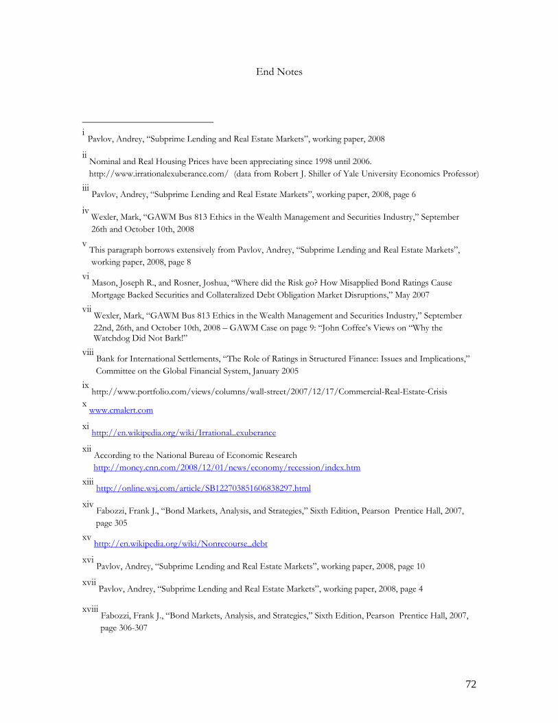
End Notes

i Pavlov, Andrey, “Subprime Lending and Real Estate Markets”, working paper, 2008

ii Nominal and Real Housing Prices have been appreciating since 1998 until 2006.

http://www.irrationalexuberance.com/ (data from Robert J. Shiller of Yale University Economics Professor)

page 6

Industry,” September

Markets”, working paper, 2008, page 8

vi , Joshua, “Where did the Risk go? How Misapplied Bond Ratings Cause

Mortgage Backed Securities and Collateralized Debt Obligation Market Disruptions,” May 2007 v

813 Ethics in the Wealth Management and Securities Industry,” September , and October 10th, 2008 – GAWM Case on page 9: “John Coffee’s Views on “Why the

Bank for International Settlements, “The Role of Ratings in Structured Finance: Issues and Implications,”

iews/columns/wall-street/2007/12/17/Commercial-Real-Estate-Crisis

iii Pavlov, Andrey, “Subprime Lending and Real Estate Markets”, working paper, 2008,

iv Wexler, Mark, “GAWM Bus 813 Ethics in the Wealth Management and Securities 26th and October 10th, 2008

v This paragraph borrows extensively from Pavlov, Andrey, “Subprime Lending and Real Estate

Mason, Joseph R., and Rosner

ii Wexler, Mark, “GAWM Bus

22nd, 26th Watchdog Did Not Bark!”

viii

Committee on the Global Financial System, January 2005

ix http://www.portfolio.com/v

x www.cmalert.com

xi http://en.wikipedia.org/wiki/Irrational_exuberance

xii According to the National Bureau of Economic Research

.com/2008/12/01/news/economy/recession/index.htm http://money.cnn

297.html

xiii http://online.wsj.com/article/SB122703851606838

” Sixth Edition, Pearson Prentice Hall, 2007,

xiv Fabozzi, Frank J., “Bond Markets, Analysis, and Strategies,

page 305

xv http://en.wikipedia.org/wiki/Nonrecourse_debt

xvi Pavlov, Andrey, “Subprime Lending and Real Estate Markets”, working paper, 2008, page 10

xvii Pavlov, Andrey, “Subprime Lending and Real Estate Markets”, working paper, 2008, page 4

xviiiFabozzi, Frank J., “Bond Markets, Analysis, and Strategies,” Sixth Edition, Pearson Prentice Hall, 2007,

page 306-307

72

http://www.cmalert.com/

http://en.wikipedia.org/wiki/Irrational_exuberance

http://online.wsj.com/article/SB122703851606838297.html

ION WORKERS (http://www.conference-board.org/aboutus/about.cfm

xix Manufacturer Average Workweek: Series Id: CES3000000007; Data Type: AVERAGE WEEKLY HOURS

OF PRODUCT ) x

://www.thestreet.com/tsc/basics/tscglossary/initialjoblessclaims.html

x http

xxi http://www.investopedia.com/university/releases/durablegoods.asp

xxii http://www.investopedia.com/terms/p/pmi.asp?viewed=1

xxiii http://www.investopedia.com/terms/h/housingstarts.asp

xxiv http://www.investopedia.com/terms/s/sp500.asp

xxv http://www.investopedia.com/terms/m/m2.asp

xxvi http://www.sca.isr.umich.edu/documents.php?c=i

xxviiPindyck, Robert S., and Rubinfeld, Daniel L., “E

conometric Models and Economic Forecasts,” Fourth

Edition, Irwin/McGraw-Hill, 1998, page 57

Pindyck, Robert S., and Rubinfeld, Daniel L., “Econometric Models and Economic Forecasts,” Fourth

“Econometric Models and Economic Forecasts,” Fourth



there were many iterations varying the size of the gap between investment d non-investment grade CMBS securities. The R^2 for the gap value equals to 10 is higher than

xxviii


xxix d Rubinfeld, Daniel L., Pindyck, Robert S., an


xxx d Rubinfeld, Daniel L., Pindyck, Robert S., an


xxxi Pindyck, Robert S., and Rubinfeld, Daniel L.,


xxxii See Table 1 in Appendix

xxxiii Table 2 in the Appendix The Rating Scale for the Gap Valuation is found in

xxxiv For Regression Model 6,

grade an the R^2 values for gap of 15 and a gap of 5, 0.555 > 0.5516 or 0.5399.

xxxv Tables 1 and 2 in the Appendix contain the actual figures used in the regression for the respective

Regression Models

73

http://www.conference-board.org/aboutus/about.cfm

http://www.thestreet.com/tsc/basics/tscglossary/initialjoblessclaims.html

http://www.investopedia.com/university/releases/durablegoods.asp

http://www.investopedia.com/terms/p/pmi.asp?viewed=1

http://www.investopedia.com/terms/h/housingstarts.asp

http://www.investopedia.com/terms/h/housingstarts.asp

http://www.investopedia.com/terms/s/sp500.asp

an analysis of traditional issue specific and ...summit.sfu.ca/system/files/iritems1/756/gawm 2008,...

Documents