predictability of hong kong stock returns by using gearing...

PREDICTABILITY OF HONG KONG STOCK RETURNS

BY USING GEARING RATIO

by

Michael Man Kit Ng Bachelor of Arts in Economics

University of Waterloo

and

Ke Wang Bachelor of Business Administration

Kwantlen University College Certified General Accountant

PROJECT SUBMITTED IN PARTIAL FULFILLMENT OF THE REQUIREMENTS FOR THE DEGREE OF

MASTER OF BUSINESS ADMINISTRATION

In the Global Asset and Wealth Management

© Michael Ng & Ke Wang

SIMON FRASER UNIVERSITY

Spring 2009

All rights reserved. This work may not be reproduced in whole or in part, by photocopy

or other means, without permission of the authors.

ii

APPROVAL

Name: Michael Ng & Ke Wang

Degree: MBA – Global Asset and Wealth Management

Title of Thesis: Predictability of Hong Kong Stock Returns by Using Gearing Ratio

Examining Committee:

______________________________________

Dr. Peter Klein Senior Supervisor Professor of Finance

______________________________________

Dr. Karel Hrazdil Second Reader Assistant Professor of Accounting

Date Defended/Approved: ______________________________________

iii

ABSTRACT

The purpose of our study is to examine the ability of the debt ratio to predict Hong Kong

stock market stock returns in long run. Our test period is from Jan 1, 1999 to May 1,

2008. Sixty companies in the Hang Seng Composite Index were included in our samples

for the research. We found Leverage ratios could not have been used to predict

cumulative abnormal returns or buy-and-hold abnormal returns in our test period. The

correlation between Leverage ratios and abnormal returns is not significant. We also

found other commonly used ratios, such as price-to-earnings ratio, price-to-book ratio

and market value are better indicators of abnormal returns than Leverage ratios.

Keywords: Capital Structure, Leverage, Abnormal Stock Returns, Debt Ratios

iv

EXECUTIVE SUMMARY

The purpose of our study is to examine the ability of debt ratios to predict Hong Kong

stock market stock returns in the long run. Our paper is based on the Muradoglu and

Wittington (2001) study of predictability of UK stock returns.

Our samples of 60 companies are selected from 198 companies of Hang Seng Composite

Index by, 1). deducting 26 companies in financial sectors, whose Leverage ratios have

different interpretations from the others; 2). deducting 80 companies that were not listed

before Jan. 1, 1999 for 10-year analysis; 3). deducting 3 companies that had changed the

fiscal period end date during the observing periods for preventing the difference in fiscal

year calculation; 4). deducting 9 companies that have important data missing or

unavailable , such as annual reports; and 5). deducting 20 companies which have

financial year ended other than Dec 31.

In contrast with the study on the U.K. market done by Muradoglu and Whittington in

2001, we find out that Leverage ratios could not have been used to predict cumulative

abnormal returns (CAR) or buy-and-hold abnormal returns (BHAR). Based on the data

we used, the correlation between Leverage Ratios and abnormal returns is not significant.

The abnormal returns show random patterns to the Leverage level in the seven 3-year

period and the overall sample.

v

We realized that other common used ratios or indicators, Price-to-Earnings ratio (P/E),

Price-to-Book ratio (P/B) and Market Value (MV), have stronger power to search for

abnormal returns than the Leverage ratio. All P/E, P/B, and MV are negatively correlated

to the abnormal returns.

We also put the Leverage, P/E, P/B, and MV in pairs for forming investment strategies.

We found out that P/B and MV are the best partners in looking for abnormal returns. Low

P/B with low MV generates the highest CAR and BHAR, and high P/B with high MV

generates the lowest CAR and BHAR. In order to receive higher than average abnormal

returns, investors would be better to look at companies with low P/E, low P/B, and low

MV. Our findings are consistent with Lam (2002). He found in his study firm size, book-

to-market and earnings-price capture cross section return variation in his test period for

the Hong Kong stock market. Our findings also are consistent with the Fama and French

(1992, 1995, and 1996). Portfolios form based on book-to-market and the size explain

return anomalies better.

vi

ACKNOWLEDGEMENTS

We would like to thank Dr. Peter Klein for his guidance and supports throughout our

project. A special thanks goes to Dr. Karel Hrazdil for his helpful insights. It has been a

privilege to work with both of them.

To my parents, my wife, Maggie, my son, Isaac, and my daughter, Arella.

M. N.

To my dear mother, who encourages and motivates me to pursue higher education.

K. W.

vii

TABLE OF CONTENTS

Approval .............................................................................................................. ii

Abstract .............................................................................................................. iii

Executive Summary .......................................................................................... iv

Acknowledgements ........................................................................................... vi

Table of Contents ............................................................................................. vii

List of Figures .................................................................................................. viii

List of Tables ..................................................................................................... ix

INTRODUCTION .................................................................................................. 1

LITERATURE REVIEW ........................................................................................ 3

Prior Research Papers on the Debt-to-equity Ratio .......................................... 3

Multifactor Explanations of Asset Pricing Anomalies ......................................... 7

Ratio Analysis on Hong Kong Stock Market ...................................................... 9

DATA AND METHODOLOGY ........................................................................... 11

FINDINGS .......................................................................................................... 20

Overall Result .................................................................................................. 20

Sub-period Results .......................................................................................... 23

Compare Our Samples with Muradoglu and Whittington’s Samples ............... 29

CONCLUSIONS ................................................................................................. 42

REFERENCE ..................................................................................................... 44

Exhibit 1 Muradoglu & Whittington Sub-period CAR & BHAR ..................... 46

viii

LIST OF FIGURES

Figure 1: The Overall CAR & BHAR ................................................................... 21

Figure 2: Scatter Diagram of the Overall CAR and Leverage ............................ 22

Figure 3: Scatter Diagram of the Overall BHAR and Leverage ......................... 23

Figure 4: Period 1 (1999-2002) CAR & BHAR .................................................... 24






Figure 10: Period 7 (2005-2008) CAR & BHAR .................................................. 27

Figure 11: Hang Seng Index and FTSE .............................................................. 30

Figure 12: P/E of the Overall Samples ............................................................... 31

Figure 13: Scatter Diagram of the Overall CAR and P/E .................................... 32

Figure 14: Scatter Diagram of the Overall BHAR and P/E .................................. 33

Figure 15: P/B of the Overall Samples ............................................................... 34

Figure 16: Scatter Diagram of the Overall CAR and P/B .................................... 35

Figure 17: Scatter Diagram of the Overall BHAR and P/B .................................. 35

Figure 18: MV of the Overall Samples ................................................................ 36

Figure 19: Scatter Diagram of the Overall CAR and MV .................................... 37

Figure 20: Scatter Diagram of the Overall BHAR and MV .................................. 37

ix

LIST OF TABLES

Table 1: Comparison of the Two Researches .................................................... 12

Table 2: Financial Year End .............................................................................. 13

Table 3: The Number of Trading Day ................................................................. 15

Table 4: Twenty-four Portfolios Based on Ratios Combinations ......................... 18

Table 5: The Overall Results .............................................................................. 21

Table 6: 7 Periods Results ................................................................................. 28

Table 7: The Correlations between Periods of Two Researches ........................ 30

Table 8: CAR by Different Combined Strategies ................................................ 39

Table 9: BHAR by Different Combined Strategies .............................................. 40

1

INTRODUCTION

For years investors have been seeking for a fast and easy way to detect future abnormal

earnings. Using financial ratios is one of the investment strategies. The ratios, book-to-

market, price-to-earnings, size, and various others were used in the previous papers to test

for their ability in predicting abnormal earnings. Some studies show the debt-to-equity

ratio has the power to forecast future abnormal earnings (Muradoglu and Wittington

2001) while others have proved that the book-to-market ratio, size and market returns

combined which are the best ways to explain abnormal earnings (Fama and French 1992).

The gearing ratio, also known as the Leverage ratio, is one of the most important ratios

for evaluating firms‟ capital structure. Several studies on the gearing ratio concluded that

it is a strong indicator for the abnormal returns in US and UK stock market

(Bhandari1988, Muradoglu and Wittington 2001). We are interested in the gearing ratio‟s

ability in predicting abnormal earnings in the Hong Kong stock market.

The research hypothesis in our paper is whether the abnormal stock returns in the Hong

Kong stock market can be predicted through the examination of the gearing ratio. Our

paper is based on the predecessors‟ paper by Muradoglu and Wittington (2001)

Predictability of UK Stock Returns by Using Leverage Ratios.

2

We chose the Hong Kong market because it is one of the major stock markets in Asia. It

has a long history, and is well regulated. Hong Kong is a gateway for foreigners to invest

in China, the world‟s fastest growth economy.

The observing period for this research is from May 1, 1999 to April 30, 2008. The raw

data starts from July 1, 1998 to September 30, 2008. The period covers 2 cycles in the

market. The market hit the lowest during the Asian financial crisis in 1998, and peaked

its highest during the dot com period of the year 2000. The market crashed again while

the SARS attacked Hong Kong in 2003, and peaked in 2007 due to the rumour that the

Chinese government would allow the people in mainland China to invest in Hong Kong

stock market.

3

LITERATURE REVIEW

In the literature review we first go over the prior research papers on the debt-to-equity

ratio and its relationship to stock abnormal earnings. We then examine the multi-factor

explanations of asset pricing anomalies. Finally, we review the literature on ratio analysis

on the Hong Kong stock market.

Prior Research Papers on the Debt-to-equity Ratio

In this section we look at the capital structure theory and the prior studies on this topic.

Modigliani and Miller (1958) capital structure irrelevance principle states in absence of

taxes, bankruptcy costs, and in a world of complete and perfect information, the value of

a firm is unaffected by the firm‟s financing decisions. It does not matter if the firm‟s

capital is raised by issuing stocks or selling debts. The higher return for the leveraged

firm‟s equity is due to the risk premium associated with the Leverage. Therefore,

according to their principle, the debt-to-equity ratio can not serve as the indicator for the

abnormal returns. However, several studies done in the past for the US and UK markets

have showed that there is a strong relationship between the debt-to-equity ratio and

common stock returns.

Bhandari (1988) tested in the paper Debt/Equity Ratio and Expected Common Stock

Returns: Empirical Evidence the relationship between ratios of debt-to-equity and

common stock returns. His data included the two years sub-periods from 1948-1949 to

4

1980 –1981 for the US stock market. The number of stocks in the sample periods range

from 331 to 1241, with an average of 728. Because the author used data from the

COMPUSTAT database, the data excluded the stocks that no longer exist at the end of

the period. The samples used in this paper are survival stocks only. The result shows that

the expected common stock returns are related to the debt-to-equity ratio. The

relationship is the strongest in January with the coefficient of 0.64 percent per month.

The estimated overall coefficient is 0.13 percent per month. Bhandari concluded in his

paper that the expected returns on common stocks are positively related to the debt/equity

ratio (Bhandari 1988). Bhandari also concluded that the premium associated with the

debt/equity ratio is not likely to be the risk premium.

Furthermore, Hull‟s 1999 paper Leverage ratio, Industry Norms, and Stock Price

Reaction: An Empirical Investigation of Stock-for-Debt Transactions also provided proof

that there is an optimal or investors‟ preferred capital. The paper tested the hypothesis

that the firms‟ debt-to-equity ratios moving toward the industry average have a positive

market response than the firms moving away from the industry average debt-to-equity

ratio.

In the paper, Hull tested 338 samples where firms‟ debt-to-equity ratios are moving

closer to or away from the industry average through common stock offering during 1970-

1988. He collected three sets of data for each of the 338 samples, pre-DE ratio, post-DE

ratio and industry average. The Pre-DE ratio is the firms‟ debt-to-equity ratio before the

result announcement. The Post-DE ratio is derived from the firm‟s Pre-DE ratio adjusted

5

for planned changes in the stock or debt in the announcement. Lastly, the industry

average is the medium DE ratio for all firms with the same Standard Industry

Classification code.

Hull studied the effect of the changes in the debt-to-equity ratio in relation to the industry

average on both short-term (-5 to + 5 days around the announcing date) and long-term (-

220 to -2 days) cumulative abnormal returns. The short-term stock return result showed

that the favourable is the “closer to” groups. The paper reported that the “closer to” group

in the 3-day average announcement period have an average of 1.5% return higher than

the “away from” group. He also looked at the cumulative stock return in excess market

return for the period from -220 to -2 days, and found the “away from” group have a lower

return than the “closer to” group.

The research result supported the hypothesis, the firms debt-to-equity ratio moving

toward the industry average have a positive market response than the firms moving away

from the industry average debt-to-equity ratio. The moving closer groups had a 1.5%

high return than the moving away groups in the 3 days average announcement period. He

further concluded that there is an optimal capital structure, and to some extent, the

industry debt-to-equity norms represent the optimal debt-to-equity ratio.

Muradoglu and companies had done several research papers on the capital structure

(debt-to-equity ratio) and abnormal returns. The first one in the series is the Predictability

of UK Stock Returns by Using Leverage Ratios (Muradoglu and Whittington 2001). Their

6

sample included the 170 companies listed at the British FTSE-350 index returns from

1990 to 1999. The companies were ranked according to the degree of the Leverage that

they had, and grouped into 10 Deciles where Decile 1 has the lowest debt-to-equity ratio

and Decile 10 has the highest ratio. Their result showed that companies with low

Leverage ratios had higher returns than the companies‟ with high Leverage ratios. In fact,

the result showed “if an investor were to invest in the first Deciles and has an average

debt burden of 3.4%, he would be able to earn a cumulative abnormal return of 13.7% in

three years time.” The authors concluded that the strategy based on the debt-to-equity

ratio would have outperformed the market during the testing period.

In Muradoglu next paper, he, Bakke and Kvernes aimed at constructing a long-term

investment strategy based on the gearing ratio. In addition to testing the gearing ratio and

its ability to predict abnormal returns, Muradoglu, Bakke and Kvernes (2005) also

conducted robustness tests on ratios, such as size, book-to-market and price-to-earnings

ratios, which influence the abnormal returns. Their sample included 52 FTSE 100 listed

companies, and excluded the financial companies for the period of 1991 to 2002. Their

result showed that companies with low gearing ratios outperform the market in long run.

Regarding the robustness tests they found out that the book-to-market ratio do not have

any significant contribution to excess returns. Low gearing ratios generates excess returns

regardless PE levels. However, a combination of the low gearing ratio and low PE

generates the highest excess returns. With regard to the size they found out that the only

portfolio which generates significantly positive excess returns was the small cap and high

gearing portfolio.

7

Muradoglu and Sivaprasad (2006) further tested the debt-to-equity ratio and the abnormal

returns in their article Capital Structure and Firm Value: An Empirical Analysis of

Abnormal Returns. In this article, they divided their samples into different risk classes

based on industry classifications. The sample included the 2637 companies listed on the

London Stock exchange from 1965 to 2004. The results were consistent with the pervious

studies. They found that, for the most risky classes, abnormal returns decrease with the

Leverage, and firms with low Leverage ratios can earn significantly high returns than the

firms with high Leverage. They also reported that, for oil, gas, and utility industries, the

abnormal earnings increased with the Leverage. Their results are robust with regard to

other factors, such as the price-to-earnings ratio, size, market risk and book value.

Multifactor Explanations of Asset Pricing Anomalies

Despite the studies discussed above, Fama and French‟s studies found that there are

multi-factors in asset return anomalies and the debt-to-equity ratio is not one of them. In

this section, we will go over Fama and French (1992), Fama and French (1995) and Fama

and French (1996) empirical researches.

Fama and French‟s (1992) paper The Cross-Section of Expected Stock Returns tested the

ability of two variables, the size and the book-to-market ratio, in explaining the variance

in stock returns associated with the market beta β, size, Leverage, book-to-market equity

and earnings-price ratios. Their data included all non-financial firms in NYSE, AMEX,

and NASDAQ for the period from 1962 – 1989. The research found that there is a strong

8

relation between stock returns and size, and the relationship between stock returns and

the book-to-market ratio was even stronger than the size to returns.

The paper reported the relationship between β and the average return disappeared in

more recent periods (it referred to 1963-1990). The test did not support the positive

relationship between the average stock returns and the β. It also pointed out that “factors

like size, E/P, Leverage, and book-to-market are all scaled version of a firm‟s stock

price…it is reasonable to expect that some of them are redundant for explaining average

returns”. In addition, the test result revealed that the combination of the size and the

book-to-market ratio is able to capture the cross-section variation in the average stock

returns.

In their 1995 paper Size and Book-to-Market factors in Earnings and Returns, Fama and

French tested the relationship between firms size and the book-to-market to stock prices

by looking at the relation between size and the book-to-market to firms earnings. The

ultimate goal for their paper is to reach a rational explanation for the significant relation

between firm size and the book-to-market to stock price. They based their test on two

hypotheses, “1, there is a common risk factors in returns associated with size and book-

to-market, and 2. the size and book-to-market patterns in returns can be explained by the

behaviour of earnings”. The result shows that size and the book-to-market are related to

firm profitability. Fama and French also found that the market and the size factors in

earnings help explain the market and the size factors in returns. However, there is no

evidence that the returns respond to the book-to-market factor in earnings. Although there

9

was no supporting evidence, the authors thought that noise is the main contributing factor

for the failure to find more evidence of common factors in earnings driving returns.

Fama and French‟s 1996 article Multifactor Explanations of Asset Pricing Anomalies

identified a three factors model, which provides explanations of asset pricing anomalies.

The three factors include the overall market excessive return, firm size and the firm‟s

book-to-equity ratio. Fama and French used the same sample in this paper as they did in

1993. The samples were divided into 25 portfolios by their sizes and book-to-market

ratios. The portfolios showed higher returns for small stocks and high returns for higher

book-to-market ratio. They concluded, “three-factor risk return relation is a good model

for the returns on portfolios formed on size and book-to-market-equity”. They also stated

that the three-factor model explains the return patterns in portfolios, which were formed

on characteristics, such as size, earnings/price, cash flow/price, book-to-market, and sales

growth. Their discovery is useful in the real world applications. Based on their test result,

forming portfolios based on the size and the book-to-market giving investors better

returns than traditional portfolios formed by the mean-variance theory.

Ratio Analysis on Hong Kong Stock Market

The literature written in English related to ratios analysis for the Hong Kong stock market

is very limited. We were only able to find one paper in English that relates to our topic.

Lam‟s (2002) paper The Relationship Between Size, Book-to-Market Equity Ratio,

Earnings–Price Ratio, and Return for the Hong Kong Stock Market studied the

relationship between the stock return and firm size, the Leverage, book-to-market ratio,

and earnings-price ratio. His study covered 100 firms continuously listed on the Hong

10

Kong Stock exchange for the period from July 1984 to June 1997. He excluded financial

firms from the study because they have on average higher Leverage ratios. The paper

followed Fama and French (1992) in defining size and variables related to accounting

information. The results were tested for sub-periods and across the months. January effect

was also tested, and the result showed that January effect does not drive the test result.

He concluded in his paper that, β is not able to explain returns. But the firm size, book-to-

market, and earnings-price capture cross section return variation in the tested period. He

reported that the book value and the Leverage can also explain the cross section variation;

however, those can be discarded because their effects are dominated by the size, book-to-

market and earning-price. In addition he suggested the three factors model (size, book-to-

market, and earning-price) to be served as the risk proxy, instead of β, for the Hong Kong

stock market. Lam suggested two practical implications for his findings. First, investors

and managers should evaluate their portfolios by comparing them with portfolios which

have similar size, book-to market equity and earning-price ratios. Second, Risk Proxy

based on the three factors can be used to measure the cost of capital when calculating the

present value of investments.

11

DATA AND METHODOLOGY

The purpose of this study is to examine the ability of debt ratios in predicting company

stock returns in the long run. We initiated the work as Muradoglu and Whittington (2001)

did for the U.K. market. They started from the FTSE-350 index, which incorporates the

largest 350 companies by capitalization, for stock picking. There are 1,090 companies

listed at the main board of Hong Kong as of November 30, 2008. The samples we use are

constituted by the companies listed in the Main Board of Hong Kong, and included in the

Hang Seng Composite Index, which is composed by about the top 200 listed companies

and worth greater than 90% of the total value of the whole Hong Kong market.

The sample covers the period from Jan. 1, 1999 to May 1, 2008. Historical prices are

available from some financial information providers, e.g. Yahoo! Finance; however, the

free data are only available up to January 1, 2003 for non blue chips companies. The

missing data could be searched from the newspaper database at any public library in

Hong Kong, or purchased from the Hong Kong Exchanges and Clearing Limited, HKEX,

or a few financial information providers, like AASTOCKS.com. The data of the

historical prices, background information, annual report announcement dates, and

outstanding shares of the companies used in this research are from the HKEX and

HKEXnews database. The data are stored in two sub-parts of the database, prior to June

25, 2007 and since June 25, 2007. We have to search both sub-parts in order to retrieve

the data we use in this research. Since companies‟ submission of soft copy of disclosures

http://www.aastocks.com/

12

to HKEX was not mandatory for some types of company information prior to February

15, 2002, some missing data of company information are from annual reports and

company websites.

The data of Debts, Price-to-Earnings, and Price-to-Book ratios come from Thomson's

Datastream; however, there are a few P/E data missing. We used the data from annual

reports and followed the definition of the ratio by Thomson‟s Datastream for calculating

the missing data. We calculated the ratios from the year (t) before the missing year (t-1)

to the year after the missing year (t+1), and compared the first and the last data to the

existing data from Thomson‟s Datastream for verification. The data of “t-1” and “t+1” we

calculated are the same as Thomson‟s Datastream given, so we use our calculation of

year (t) for the missing data.

Table 1: Comparison of the Two Researches

This table compares the two studies.

Muradoglu and

Whittington Ng and Wang Ratio

Market United Kingdom Hong Kong N/A

Period 1990/01/01 - 1999/05/01 1999/01/01 - 2008/05/01 N/A

Index FTSE-350 Hang Seng Composite

Index N/A

Samples 170 60 2.83 : 1

Listed Companies at the

Beginning of the Period 2015 680 2.96 : 1

Market Capitalization at the

Beginning of the Period1

USD 831,231,783,000 USD 343,566,500,000 2.42 : 1

1 The historical market capitalization of the Hong Kong market is from the World Federation of Exchange. The prices are quoted in

U.S. dollar. The historical market capitalization of the UK market is from the London Stock Exchange, LSE. The prices are quoted in British Pound. The historical exchange rates are from the tool FXHistory provided by Oanda Corporation.

13

The final sample, from 198 companies of the Hang Seng Composite Index, is formed by,

1). deducting 26 companies in financial sectors, whose Leverage ratios have different

interpretations from other sectors; 2). deducting 80 companies that were not listed before

Jan. 01, 1999 for 10-year analysis; 3). deducting 3 companies that had changed the fiscal

period end date during the observing periods for preventing the difference in fiscal year

calculation; and 4). deducting 9 companies that have important data missing or

unavailable, such as annual reports.

Table 2: Financial Year End

The table summarizes the financial year-ended data for the remaining 80 companies from the sample

deduction.

Financial Year-End

Number of Company Percentage

March 31st 9 11.25%

June 30th 9 11.25%

September 30th 1 1.25%

December 31st 61 76.25%

Others 0 0.00%

Total 80 100.00%

More than three-fourths of the remaining companies, 61 out of 80, or 76.25%, have a

Balance Sheet date of December 31st; 9 companies, or 11.25%, use June 30th

as the

financial year-end, 9 companies, or 11.25%, use March 31st; and 1 company, or 1.25%,

uses September 30th

. Similar to Muradoglu and Whittington (2001), we have the most

companies that have the year-end date of December 31st. Since the number „61‟ is a

prime number and is not divisible, we deducted one more company from the list so that

the remaining companies can be separated in groups. We decided to remove Swire

Pacific Limited “B” (Ticker: 00087) because it is the only B shares from the list, since

14

the data from Thomson‟s Datastream are the same in A shares and B shares and we see

that as duplication.

Our final samples are 60 companies that have year-end on December 31st with completed

ratios and stock prices data. Muradoglu and Whittington (2001) mentioned that annual

reports are announced and published in the U.K. about four months after the end of the

fiscal period in general. In Hong Kong Main Board issuers must publish annual reports

not later than 4 months after the date upon which the financial period ended. To verify

the companies announced and published their annual reports between January 1st and

April 30th

each year, we searched the HKEXnews database from the year 1998 to 2008

and confirmed that none of our samples has an annual report announcement out of the

period.

We followed Barber and Lyon (1997), Vijh(1999), and Muradoglu and Whittington

(2001) methodologies for calculating long run stock returns. 3-year stock returns for the

selected companies are calculated by the log difference of consecutive closing prices,

which are adjusted for dividends, splits and right issues, on a daily basis. There are seven

3-year periods from May 1, 1999 to April 31, 2008. We used the closing price of the last

trading day before May 1 each year for the return calculation. For those seven periods,

there are between 737 to 748 trading days. We used the minimum, 737 days, to calculate

the returns for the overall calculation, which has the comparison of returns of 420

observations from different periods.

15

Table 3: The Number of Trading Day

The number of trading day in the seven 3-year periods. We used the minimum, 737 days, for the overall

calculation.

START DATE END DATE

NO. OF TRADING

DAY

Period 1, P1 30/4/1999 30/4/2002 737

Period 2, P2 30/4/2000 30/4/2003 738

Period 3, P3 30/4/2001 30/4/2004 741

Period 4, P4 30/4/2002 30/4/2005 748

Period 5, P5 30/4/2003 30/4/2006 742

Period 6, P6 30/4/2004 30/4/2007 742

Period 7, P7 30/4/2005 30/4/2008 742

Our research starts with the Leverage ratio. The methodology, presenting the evidence at

the portfolio level, is the same as the one in Muradoglu and Whittington (2001). Sixty

companies are ranked by the Leverage ratio and sorted into Deciles. The Capital Gearing

Ratio (Data-stream code: 731) which Muradoglu and Whittington (2001) used is defined

as:

Gearing Ratio = Preferred Shares + Subordinated Debt + Total Loans + Short-term Loans

--------------------------------------------------------------------------------------------------------

Total Capital Employed + Short-term Debt + Intangible Assets + Future Tax Liabilities

We have 60 data for each of the 7 periods, and 420 observations for the overall

calculation. We divided the 60 samples from each period into 10 groups with 6

companies each for the yearly analysis, and divided the 420 observations into 10 groups

for the overall calculation. We put the companies into the Deciles starting from the

lowest Leverage ratio to the highest Leverage ratio. Therefore, the companies with the

lowest Leverage ratio go into Decile 1 and the companies with the highest Leverage ratio

go into Decile 10.

16

The Price-to-Earnings ratio, the Price-to-Book ratio, and the Market Value of the

companies are also used in the analysis. At May 1 of year t, the information we use are

P/E(t-1), P/B(t-1), and MV(April 30, t). The definitions of P/E and P/B are from

Thomson‟s Datastream.

P/E(i,t-1) = Closing Price of i on the last trading day in year t-1

--------------------------------------------------------------

Earning Per Share as reported for i

P/B(i,t-1) = Market Cap of i on the last trading day in year t-1

-----------------------------------------------------------------

Common Equity of i on the last trading day in year t-1

MV (i,April 30, t) = Outstanding Shares of i * Closing Price at April 30 of year t

We followed the methods in Barber and Lyon (1997) and Vijh(1999) to calculate the

three-year cumulative abnormal returns, CAR, the three-year buy and hold abnormal

returns, BHAR, and the test statistics. The equation of the market adjusted abnormal

returns is:

AR(it) = R(it) – R(mt), for day t

17

R(it) is the return of the company i for day t, and R(mt) is the return of the market, the

Hang Seng Index, HSI, for day t. The returns are calculated from the log differences of

two consecutive prices, that is, ln((P(t)/P(t-1)).

The cumulative abnormal returns, CAR, for company i are calculated by:

CAR(it) = ∑ AR(it), t = 1 to 737

The Buy-and-hold abnormal returns, BHAR, for company i are calculated by:

BHAR(it) = (∏ (1 + AR(it))) – 1, t = 1 to 737

The formulas of test statistics for testing the null hypothesis, that the mean cumulative or

buy-and-hold abnormal returns are equal to zero, are:

T(CAR) = CAR(it) / (σ(CAR(it) / √n)

T(BHAR) = BHAR(it) / (σ(BHAR(it) / √n)

n is the number of companies and CAR(it) and BHAR(it) are the sample average.

σ(CAR(it)) and σ(BHAR(it)) are the sample standard deviations of abnormal returns for

the sample of n companies.

18

We are also interested in understanding ratio combinations in finding excessive returns.

Muradoglu, Bakke, and Kvernes (2005) combined the Leverage ratio with P/E, Book-to-

market, and MV for finding the best pair ratios that generated the most excessive returns.

Table 4: Twenty-four Portfolios Based on Ratios Combinations

Twenty-four portfolios are formed by the combination of the level of the Leverage, P/E, P/B, and MV.

1st Ratio 2nd Ratio

Low Leverage Low P/E

Low Leverage High P/E

High Leverage Low P/E

High Leverage High P/E

Low Leverage Low P/B

Low Leverage High P/B

High Leverage Low P/B

High Leverage High P/B

Low Leverage Low MV

Low Leverage High MV

High Leverage Low MV

High Leverage High MV

Low P/E Low P/B

Low P/E High P/B

High P/E Low P/B

High P/E High P/B

Low P/E Low MV

Low P/E High MV

High P/E Low MV

High P/E High MV

Low P/B Low MV

Low P/B High MV

High P/B Low MV

High P/B High MV

In this study, we replaced the Book-to-market, with P/B. P/B is the reciprocal of B/M,

and is readily available. We extended the work to group P/E, P/B, and MV. For ratios

combination calculations we divided the 420 overall observations into two groups by the

level of a ratio, the 1st ratio. Each group has 210 observations. The 210 observations with

the low ratio go into the low group, and the rest of the 210 observations with the high

19

ratio go into the high group. We then divided each group into two sub-groups by sorting

the second ratio. There are 24 sub-groups within these combinations. Table 4 above

shows the list of these 24 groups.

20

FINDINGS

Overall Result

The overall results are presented in Table 6. For the overall sample, the average Leverage

ratio for Decile 1 to Decile 10 are 1.9%, 9.8%, 15.1%, 20.5%, 25.2%, 29.2%, 32.9%,

38.2%, 43.7%, and 65.4% respectively. The standard deviations are 2.1%, 1.9%, 1.6%,

1.3%, 1.4%, 1.3%, 1.3%, 1.6%, 2.0%, and 22.2% respectively. The standard deviation in

Decile 10 is the highest among other Deciles. It shows that the samples in Decile 10 are

dispersed.

Unlike the finding of Muradoglu & Whittington, there is no obvious relation between

CAR and BHAR and the debt-to-equity ratio. The levels of CAR and BHAR do not seem

to follow the increase or decrease of the debt-to-equity ratio. Moving from Decile 1 to 3,

the abnormal returns seem to decrease with the increase in the debt-to-equity ratio. From

Decile 3 to 5 the abnormal returns increase with the increase in the debt-to-equity ratio.

The abnormal returns reduce again from Decile 5 to Decile 6. Lastly, the abnormal

returns seem to be the highest and increase the most when the debt-to-equity ratio

increased from Decile 7 (average ratio 32.8%) to Decile 10 (average ratio 65.4%).

Since there is no particular correlation for the level of CAR or BHAR with the increase or

decrease in the debt-to-equity ratio, we conclude that the debt-to-equity ratio is not able

to explain the Hong Kong stock market abnormal returns for the period from 1999-2008.

21

Figure 1: The Overall CAR & BHAR

Figure 1 shows the relationship between CAR & BHAR and the debt-to equity ratio. The companies with

the lowest Leverage ratio go into Decile 1 and the companies with the highest Leverage ratio go into Decile

10.

T he Ov erall C AR & B HAR

0

0.2

0.4

0.6

0.8

1

1.2

1 2 3 4 5 6 7 8 9 10

Deciles

Ab

no

rma

l R

etu

rns

CAR

BHAR

Table 5: The Overall Results

The columns represent the average Leverage ratio, CAR, T-stat of the CAR, BHAR, T-stat of the BHAR,

P/E(t-1), P/B(t-1), and MV for the Deciles.

Leverage (t-1) CAR

T-Stat (CAR) BHAR

T-Stat (BHAR) P/E(t-1) P/B(t-1) MV

Decile 1 1.9 0.5 5.4 0.4 3.8 13.6 2.3 12,620.2

Decile 2 9.8 0.3 3.6 0.3 2.4 15.4 2.4 52,047.0

Decile 3 15.1 0.3 2.7 0.4 2.4 25.8 2.3 71,102.2

Decile 4 20.5 0.4 4.4 0.5 2.9 19.6 1.1 33,618.1

Decile 5 25.2 0.4 3.7 0.6 2.4 9.4 1.1 28,456.9

Decile 6 29.2 0.2 1.9 0.3 1.1 14.9 1.2 47,571.9

Decile 7 32.9 0.4 4.0 0.3 2.5 15.9 1.1 14,157.4

Decile 8 38.2 0.4 3.9 0.4 2.8 19.0 1.3 21,579.7

Decile 9 43.7 0.5 3.8 0.7 3.1 22.2 2.0 28,540.4

Decile 10 65.4 0.6 4.5 1.0 3.4 4.4 1.9 8,878.8

Our finding is different from the result of Muradoglu and Whittington‟s paper.

Muradoglu and Whittington, using U.K. data, found out that a decreasing trend exists as

the Leverage ratio increases from Decile 1 to Decile 8, and the abnormal returns increase

from Decile 8 to Decile 10, which are the classes for companies that have the highest

Leverage. In our overall samples, the abnormal returns go up and down from Decile 1 to

22

Decile 6, then increase from Decile 7 to Decile 10. Decile 10, the group for companies

with the highest Leverage, has the most abnormal returns. Notes that the gap between

CAR and BHAR increases from Decile 8 to Decile 10. The standard deviations of the

BHAR in Decile 9 and 10 are large as well (Decile 9: 1.45, Decile 10: 1.95).

We also examined the existence of the link between the Leverage and the abnormal

returns. We plotted the 420 observations into scatter diagrams for understanding the

relationship between Leverage and the CAR and BHAR in Hong Kong market. The

graphing tool generated the regression lines. The slopes of the trend lines (CAR: 0,

BHAR: 0.004) tell us that the Leverage level does not have any meaning to cumulative

abnormal returns and is little related to buy-and-hold abnormal returns. For a 10%

increase in Leverage, there is a 4% increase in BHAR.

Figure 2: Scatter Diagram of the Overall CAR and Leverage

The slope of the trend line is 0.0002. The Leverage level does not have any meaning to the cumulative

abnormal returns, CAR.

Overall CAR & the Leverage

y = 0.0002x + 0.3907

R2 = 2E-05

-3

-2

-1

0

1

2

3

4

0 20 40 60 80 100 120 140

The Leverage

CA

R

23

Figure 3: Scatter Diagram of the Overall BHAR and Leverage

The slope of the trend line is 0.004. The Leverage level is merely related to the buy-and-hold abnormal

returns. For a 10% increase in Leverage, there is a 4% increase in BHAR.

Overall BHAR & the Leverage

y = 0.004x + 0.389

R2 = 0.0033

-2

0

2

4

6

8

10

12

14

0 20 40 60 80 100 120 140

The Leverage

BH

AR

Sub-period Results

Figure 4 to Figure 10 summarize the abnormal returns with ratios of 10 Deciles in 7

periods. We present the result in numeral form in Table 6 with other ratios. The Deciles

in each period are sorted by the Leverage ratio from the lowest to highest. There is

neither a strong evidence that the Leverage ratio is negatively correlated to both abnormal

returns, nor a common pattern on the relation of the Leverage and both abnormal returns

for all periods. For comparison we include Muradoglu and Whittington‟s sub-period

results in Appendix 1.

24

Figure 4: Period 1 (1999-2002) CAR & BHAR

The CAR and BHAR for Period 1, 1999-2002.

P1 CAR & BHAR

-0.6

-0.4

-0.2

0.0

0.2

0.4

0.6

0.8

1.0

1.2

1 2 3 4 5 6 7 8 9 10

DE C IL E S

Ab

no

rmal

Ret

urn

s

CAR

BHAR

The result in Period 1 is similar to the overall result. As the Figure shows, the CAR and

BHAR increase or decrease out of step with the Deciles, except for the Deciles 8 to 10. In

Deciles 8 to 10, the returns increase as the Leverage ratio increases.


In period 2 the returns peaked at Decile 5 and Decile 9.

P2 CAR & BHAR

-0.5

0.0

0.5

1.0

1.5

2.0

2.5

1 2 3 4 5 6 7 8 9 10

DE C IL E S

Ab

no

rmal

Ret

urn

s

CAR

BHAR

25


Period 3 is similar to period 1 and the overall result. The returns peak at Decile 4 and Decile 10. There

seems to be a relationship between the returns and the Leverage ratio in Decile 7 to 10.

P3 CAR & BHAR

0.0

0.5

1.0

1.5

2.0

2.5

3.0

1 2 3 4 5 6 7 8 9 10

DE C IL E S

Ab

no

rmal

Ret

urn

s

CAR

BHAR


Figure 7 reports the returns decrease from Decile 1 to 2 and increase from Decile 2 to 3. The returns drop to

the lowest level in Decile 6 and peak at Decile 10.

P4 CAR & BHAR

0.0

0.2

0.4

0.6

0.8

1.0

1.2

1.4

1.6

1.8

1 2 3 4 5 6 7 8 9 10

DE C IL E S

Ab

no

rmal

Ret

urn

s

CAR

BHAR

26


In period 5 the portfolio of Decile 6, with an average 30.2% of the Leverage ratio, earns the highest returns.

P5 CAR & BHAR

0.0

0.5

1.0

1.5

2.0

2.5

3.0

1 2 3 4 5 6 7 8 9 10

DE C IL E S

Ab

no

rma

l R

etu

rns

CAR

BHAR


Period 6 reports a completely different result from the overall, Period 1, and Period 3 results. Decile 3 earns

the highest returns, and the returns decline with the increase in the Leverage ratio. The returns rise from the

bottom Decile 7 to Decile 10.

P6 CAR & BHAR

-0.2

0.0

0.2

0.4

0.6

0.8

1.0

1 2 3 4 5 6 7 8 9 10

DE C IL E S

Ab

no

rma

l R

etu

rns

CAR

BHAR

27


Figure10 shows strong evidence that there is no relationship between CAR & BHAR and the Leverage

ratio. CAR and BHAR raise and fall eight times in period 7. The Figure shows that the CAR and BHAR do

not follow the changes in the Leverage.

P7 CAR & BHAR

-0.3

-0.2

-0.1

0.0

0.1

0.2

0.3

0.4

1 2 3 4 5 6 7 8 9 10

DE C IL E S

Ab

no

rma

l R

etu

rns

CAR

BHAR

All figures in Period 2 to 7 (Figure 5 to 10) have unique shapes. They do not provide any

evidence that CAR and BHAR are related to the debt-to-equity ratio. In Period 2 (Figure

5) the companies in Decile 5 and Decile 9 have the most abnormal returns. Period 3

(Figure 4) is similar to period 1 and the overall result. The firms with the highest debt-to-

equity ratio produce the largest abnormal returns. In Period 4 the returns decrease from

Decile 1 to 2 and increase from Decile 2 to 3. The returns drop to the lowest level in

Decile 6 and peak at Decile 10. In Period 5 the portfolio of Decile 6, with an average

30.2% of the Leverage ratio, earns the highest returns. Period 6‟s Decile 3 earns the

highest returns, and the returns decline with the increase in the Leverage ratio. The

returns rise from the bottom Decile 7 to Decile 10. Period 7 has a different result. Decile

3 and 4 are the best performers with the highest CAR and BHAR. There are a few times

that the CAR and BHAR have big differences in all periods. The standard deviations of

BHAR in those times are high (Period 2 – Decile 5: 3.66, Period 3 – Decile 10: 3.60,

28

Period 4 – Decile 10: 2.58, Period 5 – Decile 6: 4.59). In our research there is no

evidence that the debt-to-equity ratio is a good indicator of finding abnormal earnings.

Table 6: 7 Periods Results

The columns represent the average Leverage ratio, CAR, T-stat of the CAR, BHAR, T-stat of the BHAR,

P/E(t-1), P/B(t-1), and MV for the Deciles in 7 periods. P1 (1999-

2002) Leverage (t-1) CAR

T-Stat (CAR) BHAR


Decile 1 3.5 0.2 1.5 0.0 -0.3 13.1 1.7 24,298.4

Decile 2 11.4 0.3 1.1 0.0 0.1 12.8 2.1 65,736.2

Decile 3 16.8 0.2 1.0 0.0 -0.3 12.4 1.0 36,037.6

Decile 4 22.4 0.5 2.5 0.3 1.3 6.8 0.8 11,149.3

Decile 5 27.3 0.3 1.1 0.3 0.6 10.0 0.8 12,095.2

Decile 6 30.2 0.1 0.8 -0.1 -1.1 10.0 0.9 8,226.2

Decile 7 34.3 0.4 2.5 0.1 0.8 30.8 2.3 29,897.9

Decile 8 39.4 -0.4 -1.5 -0.5 -3.4 17.0 0.9 6,068.2

Decile 9 45.3 0.3 1.0 0.0 0.1 35.8 1.3 49,354.7

Decile 10 59.3 0.9 2.9 1.0 2.4 -21.1 1.2 11,057.9

P2 (2000-


T-Stat (CAR) BHAR


Decile 1 2.3 0.9 7.4 1.0 4.6 11.8 1.4 9,129.7

Decile 2 11.2 0.6 1.6 0.9 1.2 22.8 3.7 55,611.9

Decile 3 16.2 -0.1 -0.2 0.1 0.4 58.2 5.1 222,385.7

Decile 4 19.6 0.5 1.8 0.4 1.0 15.6 0.9 11,853.2

Decile 5 23.3 0.9 2.0 2.1 1.4 39.2 0.8 3,668.2

Decile 6 28.6 0.1 0.5 0.0 -0.3 32.5 1.0 92,727.3

Decile 7 33.4 0.3 1.2 0.2 0.8 11.4 0.9 22,518.9

Decile 8 38.0 0.8 3.4 1.0 1.8 5.3 0.6 3,425.6

Decile 9 42.4 1.0 2.1 1.8 1.7 42.7 6.3 10,680.0

Decile 10 54.9 1.0 4.6 1.2 3.1 5.5 1.2 12,559.7

P3 (2001-


T-Stat (CAR) BHAR


Decile 1 0.5 0.8 6.7 0.9 4.1 7.6 1.1 4,207.1

Decile 2 8.6 0.3 1.4 0.4 1.1 20.0 5.1 66,807.3

Decile 3 14.8 0.3 6.3 0.3 3.8 13.3 0.8 14,316.4

Decile 4 20.5 0.9 3.8 1.2 2.6 8.4 0.4 3,611.6

Decile 5 27.4 0.3 1.1 0.3 0.9 17.9 0.8 23,550.2

Decile 6 30.8 0.1 0.4 0.0 0.1 24.6 2.3 194,675.1

Decile 7 33.3 0.5 1.6 0.5 1.3 11.6 1.1 9,091.6

Decile 8 37.6 0.6 2.6 0.6 1.8 12.7 1.0 22,112.5

Decile 9 43.4 0.8 2.6 0.9 1.7 13.9 1.0 3,492.0

Decile 10 69.6 1.0 2.2 2.6 1.8 1.4 -0.3 8,254.8

P4 (2002-


T-Stat (CAR) BHAR


Decile 1 1.1 0.4 2.7 0.3 1.6 15.4 2.4 11,432.1

Decile 2 7.7 0.3 1.6 0.2 1.2 12.9 2.2 19,928.3

Decile 3 14.7 0.6 1.6 0.9 1.4 15.4 1.0 50,273.5

Decile 4 20.7 0.4 1.1 0.9 1.0 9.7 1.4 89,032.3

Decile 5 24.0 0.3 2.4 0.2 1.4 15.1 0.8 16,542.8

Decile 6 28.4 0.1 1.7 0.0 0.6 13.5 0.8 25,891.1

29

Decile 7 32.3 0.6 1.6 0.8 1.2 30.4 1.0 6,605.3

Decile 8 35.9 0.5 1.8 0.6 1.6 18.7 0.9 54,284.2

Decile 9 42.3 0.6 2.0 0.7 1.6 19.3 1.0 13,295.5

Decile 10 70.0 0.8 1.9 1.6 1.5 10.1 -1.1 5,957.1

P5 (2003-


T-Stat (CAR) BHAR


Decile 1 2.1 0.7 2.3 0.9 1.9 13.7 2.0 10,171.4

Decile 2 9.1 0.3 1.4 0.4 0.9 11.8 1.9 14,824.9

Decile 3 13.9 0.3 1.9 0.2 1.7 9.7 0.6 28,143.0

Decile 4 21.2 0.3 1.6 0.2 1.4 10.8 1.1 69,282.8

Decile 5 25.4 0.3 1.2 0.4 1.0 22.6 1.2 20,144.1

Decile 6 30.1 1.1 2.3 2.8 1.5 8.6 0.5 13,930.6

Decile 7 32.1 0.2 1.1 0.1 0.6 9.2 1.0 7,187.8

Decile 8 38.4 0.4 1.6 0.4 1.1 13.8 1.2 34,653.9

Decile 9 42.1 0.4 1.9 0.3 1.2 10.9 1.1 9,314.2

Decile 10 66.6 0.6 2.6 0.7 2.0 8.3 -1.1 4,405.1

P6 (2004-


T-Stat (CAR) BHAR


Decile 1 2.5 0.1 0.6 0.1 0.3 20.7 4.4 19,885.6

Decile 2 10.3 0.1 0.4 0.0 0.2 14.8 1.6 47,195.2

Decile 3 14.9 0.7 2.4 0.9 2.1 19.6 2.2 75,791.0

Decile 4 20.1 0.5 1.9 0.6 1.5 22.1 1.7 15,229.1

Decile 5 25.0 0.2 0.8 0.3 0.8 -13.1 1.0 28,994.1

Decile 6 28.1 0.2 1.0 0.1 0.7 14.6 1.3 21,120.8

Decile 7 33.8 0.1 0.6 0.0 -0.4 15.9 1.6 22,959.0

Decile 8 39.6 0.3 1.0 0.4 0.8 22.4 2.1 8,014.6

Decile 9 44.8 0.3 1.4 0.3 1.2 24.0 1.7 53,248.6

Decile 10 69.6 0.4 1.8 0.3 1.8 8.4 11.2 7,475.4

P7 (2005-


T-Stat (CAR) BHAR


Decile 1 1.8 -0.1 -0.8 -0.2 -2.3 17.4 4.0 20,354.6

Decile 2 10.6 0.1 1.0 0.0 0.0 12.4 1.4 48,690.6

Decile 3 15.0 -0.1 -0.3 0.0 -0.1 49.8 3.0 111,063.7

Decile 4 19.3 0.2 0.9 0.2 0.7 16.7 1.5 24,946.3

Decile 5 24.1 0.0 0.0 -0.1 -0.9 15.1 1.4 27,944.0

Decile 6 27.4 0.1 0.2 0.1 0.3 11.2 1.2 17,091.6

Decile 7 30.9 0.2 0.7 0.4 0.7 15.0 1.6 36,974.9

Decile 8 38.6 0.0 0.0 0.0 -0.1 17.3 2.1 20,114.8

Decile 9 46.3 0.1 0.2 0.3 0.5 18.1 1.1 57,892.5

Decile 10 66.4 -0.1 -0.2 0.1 0.2 14.2 1.9 11,122.2

Compare Our Samples with Muradoglu and Whittington’s Samples

For better understanding the difference in the results, we compared the Hong Kong stock

market returns in our test period, April 30, 1999 to April 30, 2008, with the UK Stock

market returns in Muradogle and Whittington‟s (2001) test period, April 30, 1990 to

30

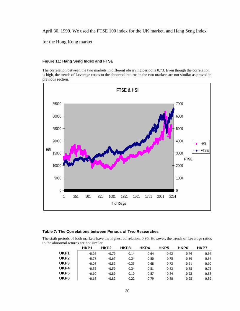
April 30, 1999. We used the FTSE 100 index for the UK market, and Hang Seng Index

for the Hong Kong market.

Figure 11: Hang Seng Index and FTSE

The correlation between the two markets in different observing period is 0.73. Even though the correlation

is high, the trends of Leverage ratios to the abnormal returns in the two markets are not similar as proved in

previous section.

FTSE & HSI

0

5000

10000

15000

20000

25000

30000

35000

1 251 501 751 1001 1251 1501 1751 2001 2251

# of Days

HSI

0

1000

2000

3000

4000

5000

6000

7000

FTSE

HSI

FTSE

Table 7: The Correlations between Periods of Two Researches

The sixth periods of both markets have the highest correlation, 0.95. However, the trends of Leverage ratios

to the abnormal returns are not similar.

HKP1 HKP2 HKP3 HKP4 HKP5 HKP6 HKP7

UKP1 -0.26 -0.79 0.14 0.64 0.62 0.74 0.64

UKP2 -0.78 -0.67 0.34 0.80 0.75 0.89 0.84

UKP3 -0.08 -0.82 -0.35 0.68 0.73 0.61 0.60

UKP4 -0.55 -0.59 0.34 0.51 0.83 0.85 0.75

UKP5 -0.60 -0.89 0.10 0.87 0.84 0.93 0.88

UKP6 -0.68 -0.82 0.22 0.79 0.88 0.95 0.89

31

The correlation between the two markets in the two observing period is 0.73. Even

though the correlation is high, the trends of Leverage ratios to the abnormal returns in the

two markets are not similar. If we compare the markets by periods, as Table 7 shows, the

sixth periods of both markets have the highest correlation, 0.95. However, the trends of

Leverage ratios to the abnormal returns are not similar.

Strategies Based on Multiple Ratios

Since our research shows that the gearing ratio is not a powerful tool to explain the

abnormal returns in the Hong Kong stock market, we added other ratios in this study to

see their abilities in finding excessive returns. Before this, we looked at the relationship

between the Leverage and the other ratios. The ratios that we added are the Price-to-

earnings ratio (P/E), the Price-to-book ratio (P/B), and the Market Value (MV).

Figure 12: P/E of the Overall Samples

The relationship between the P/E (t-1) and the levels of the debt-to-equity ratio.

P/E(t-1)

0

5

10

15

20

25

30

1 2 3 4 5 6 7 8 9 10

Deciles

P/E (t-1)

P/E(t-1)

32

The data of P/E is from Thomson‟s Datastream. We used P/E(t-1) for year t calculation.

The average P/E for Decile 1 to 10 are 13.6x, 15.4x, 25.8x, 19.6x, 9.4x, 14.9x, 15.9x,

19.0x, 22.2x, and 4.4x respectively. Note that the companies in Decile 10 have the lowest

average P/E and the companies in Decile 3 have the highest. From Figure 12 we saw that

the relationship between the Leverage and the P/E is about a M-shape. P/E increases as

the Leverage increases from Decile 1 to 3. P/E decreases from the highest, Decile 3, to

Decile 5, and increase again to Decile 9. For the companies with the highest Leverage,

their P/E is the lowest.

Figure 13: Scatter Diagram of the Overall CAR and P/E

The relationship between the P/E and the cumulative abnormal returns. For a 10x increase in the P/E, the

CAR decrease by 4%.

Overall CAR & P/E

y = -0.004x + 0.4594

R2 = 0.0232

-3

-2

-1

0

1

2

3

4

-200 -150 -100 -50 0 50 100 150 200 250

P/E (t-1)

CAR

33

Figure 14: Scatter Diagram of the Overall BHAR and P/E

The relationship between the P/E and the buy-and-hold abnormal returns. For a 10x increase in the P/E, the

BHAR decreases by 5%.

Overall BHAR & P/E

y = -0.0057x + 0.5942

R2 = 0.0128

-2

0

2

4

6

8

10

12

14

-200 -150 -100 -50 0 50 100 150 200 250

P/E (t-1)

BHAR

We then looked at the P/E ratio to the abnormal returns. From the above two Figures, we

saw that there is a negative relationship between P/E and the abnormal returns. The lower

the P/E, the higher the abnormal returns, and vice versa. For a 10x increase in P/E, the

CAR decreases by 4% and the BHAR decreases by 5%.

34

Figure 15: P/B of the Overall Samples

The relationship between the P/B (t-1) and the levels of the debt-to-equity ratio.

P/B(t-1)

0

0.5

1

1.5

2

2.5

3

1 2 3 4 5 6 7 8 9 10

Deciles

P/B (t-1)

P/B(t-1)

The data of P/B is from Thomson‟s Datastream as well. We used P/B(t-1) for year t

calculation. The average P/B for Decile 1 to 10 are 2.3x, 2.4x, 2.3x, 1.1x, 1.1x, 1.2x, 1.1x,

1.3x, 2.0x, and 1.9x respectively. From Decile 1 to 3, P/Bs are the highest among others.

P/Bs are low from Decile 4 to Decile 7. The P/B increases from Decile 8 and stay high at

Decile 9 and 10. Decile 2 has the highest and Decile 5 has the lowest average P/B. From

the above Figure, we see that the relationship between the Leverage and the P/B is about

a U-shape. The P/B is high when the company has very low or high Leverage, and the

P/B is low when the Leverage is moderate.

35

Figure 16: Scatter Diagram of the Overall CAR and P/B

The relationship between the P/B and the cumulative abnormal returns. For a 1x increase in the P/B, the

CAR decreases by 2%.

Overall CAR & P/B

y = -0.0204x + 0.4292

R2 = 0.0138

-3

-2

-1

0

1

2

3

4

-20 -10 0 10 20 30 40 50 60 70

P/B (t-1)

CAR

Figure 17: Scatter Diagram of the Overall BHAR and P/B

The relationship between the P/B and the buy-and-hold abnormal returns. For a 1x increase in the P/B, the

BHAR decrease by 2.8%.

Overall BHAR & P/B

y = -0.0288x + 0.5504

R2 = 0.0074

-2

0

2

4

6

8

10

12

14

-20 -10 0 10 20 30 40 50 60 70

P/B (t-1)

BHAR

36

Next, we looked at the P/B ratio to the abnormal returns. From the above two Figures, we

see that there is a negative relationship between the P/B and the abnormal returns. The

lower the P/B, the higher the abnormal returns, and vice versa. For a 1x increase in the

P/B, the CAR decreases by 2% and the BHAR decrease by 2.8%.

Figure 18: MV of the Overall Samples

The relationship between the Market Value and the levels of the debt-to-equity ratio.

MV

0

10000

20000

30000

40000

50000

60000

70000

80000

1 2 3 4 5 6 7 8 9 10

Deciles

MV HK$

MV

We calculated the market value from the method we stated above in “Data and

Methodology”. We used the MV(April 30, year t) for year t calculation. The averages

MV for Decile 1 to 10 are 12,620.23, 52,046.98, 71,102.21, 33,618.12, 28,456.92,

47,571.88, 14,571.43, 21,579.71, 28,540.38, and 8,878.81 respectively (in millions Hong

Kong dollar). The average MV increases from Decile 1 to 3. There is a weak downward

trend from Decile 3 to 10. Large companies tend to have low to moderate level of debt,

and small companies tend to have either high or low debt.

37

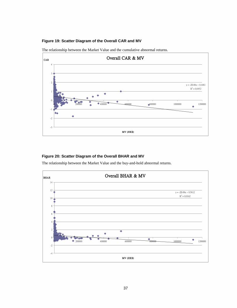
Figure 19: Scatter Diagram of the Overall CAR and MV

The relationship between the Market Value and the cumulative abnormal returns.

Overall CAR & MV

y = -2E-06x + 0.4461

R2 = 0.0452

-3

-2

-1

0

1

2

3

4

0 200000 400000 600000 800000 1000000 1200000

MV (HK$)

CAR

Figure 20: Scatter Diagram of the Overall BHAR and MV

The relationship between the Market Value and the buy-and-hold abnormal returns.

Overall BHAR & MV

y = -2E-06x + 0.5612

R2 = 0.0162

-4

-2

0

2

4

6

8

10

12

14

0 200000 400000 600000 800000 1000000 1200000

MV (HK$)

BHAR

38

The last one we looked at is the MV to the abnormal returns. From the above two Figures,

we also see that there is a negative relationship between the MV and the abnormal returns.

The lower the MV, the higher the abnormal returns, and vice versa. From the scatter

graphs, we found out that the P/E, the P/B, and the MV are useful in finding abnormal

returns.

We compared the usefulness of the ratios by combining any two of the ratios to form

portfolios. The original idea was from Muradoglu, Bakke, and Kvernes (2005). On top of

the comparison of gearing ratio with other ratios, we extended it to the comparison

between the P/E, the P/B, and the MV.

39

Table 8: CAR by Different Combined Strategies

The cumulative abnormal returns and the T-stat of the combined strategies.

CAR T-stat (CAR)

Low P/E, Low MV 89.8% 12.48

Low P/B, Low MV 89.6% 13.63

High Leverage, Low MV 81.2% 11.68

Low P/E, Low P/B 66.8% 9.32

Low Leverage, Low MV 63.3% 9.71

High Leverage, Low P/B 61.1% 8.67

High Leverage, Low P/E 59.2% 7.58

Low Leverage, Low P/E 53.7% 8.51

Low Leverage, Low P/B 53.6% 8.83

Low P/E, High P/B 45.8% 6.66

High P/B, Low MV 43.3% 6.04

High P/E, Low MV 42.4% 6.83

High P/E, Low P/B 38.1% 6.74

Low P/B, High MV 27.1% 5.84

High Leverage, High P/E 23.4% 3.81

Low P/E, High MV 22.8% 4.35

Low Leverage, High P/B 22.0% 3.80

Low Leverage, High P/E 21.9% 3.97

High Leverage, High P/B 21.5% 3.12

Low Leverage, High MV 12.3% 2.74

High P/E, High P/B 7.5% 1.32

High P/E, High MV 3.2% 0.68

High Leverage, High MV 1.3% 0.26

High P/B, High MV -1.9% -0.40

We first tested the cumulative abnormal returns. The results are listed and sorted by the

CAR, from the highest to the lowest, at the table above. The top three winners are Low

P/E & Low MV (89.8%), Low P/B & Low MV (89.6%), and High Leverage & Low MV

(81.2%). All three combinations have Low Market Value strategy. The top three losers

are High P/B & High MV (-1.9%), High Leverage & High MV (1.3%), and High P/E &

High MV (3.2%). All three combinations have High Market Value strategy.

40

From the combinations in the list, we see that low P/E and low P/B, besides low MV, are

the characteristics that generate high abnormal incomes, and vice versa. We also see High

Leverage and Low Leverage at both sides of abnormal returns. If we divide the table in

two parts, we would see High or Low Leverage with Low P/E, Low P/B, or Low MV at

the top half, and see High or Low Leverage with High P/E, High P/B, or High MV at the

bottom half. Market Value, MV, seems to be the best ratio compared to others for

searching stocks with high cumulative abnormal returns. The Leverage in our research is

not a strong indicator of finding abnormal returns.

Table 9: BHAR by Different Combined Strategies

The buy-and-hold abnormal returns and the T-stat of the combined strategies.

BHAR T-stat (BHAR)

Low P/E, Low MV 137.9% 6.81

Low P/B, Low MV 120.4% 7.20

High Leverage, Low MV 113.8% 6.21

Low P/E, Low P/B 93.4% 5.47

High Leverage, Low P/E 92.0% 4.95

High Leverage, Low P/B 80.9% 4.93

Low Leverage, Low MV 78.6% 5.80

Low P/E, High P/B 65.5% 4.36

Low Leverage, Low P/B 64.5% 5.13

High P/B, Low MV 62.2% 3.98

Low Leverage, Low P/E 53.7% 5.12

High P/E, Low MV 41.0% 4.45

High P/E, Low P/B 36.2% 4.55

High Leverage, High P/B 31.3% 2.55

Low Leverage, High P/B 24.3% 2.95

Low Leverage, High P/E 21.8% 3.01

Low P/B, High MV 21.3% 3.38

Low P/E, High MV 21.0% 3.13

High Leverage, High P/E 20.2% 2.57

Low Leverage, High MV 10.2% 1.94

High P/E, High P/B 5.9% 0.87

High P/E, High MV 1.1% 0.25

High Leverage, High MV -1.5% -0.27

High P/B, High MV -2.8% -0.63

41

We then studied the buy-and-hold abnormal returns. The results are listed and sorted by

the BHAR, from the highest to the lowest, at the table above. The top three winners are

Low P/E & Low MV (137.9%), Low P/B & Low MV (120.4%), and High Leverage &

Low MV (113.8%). Low Market Value strategy is used in all three combinations. The top

three losers are High P/B & High MV (-2.8%), High Leverage & High MV (-1.5%), and

High P/E & High MV (1.1%). High Market Value strategy is used in all three

combinations. The rankings of both the winners and losers are the same as the ones in

CAR.

From the combinations in the list, we also see that low P/E and low P/B, besides low MV,

are the characteristics that generate high abnormal incomes, and vice versa. We also see

High Leverage and Low Leverage at both sides of abnormal returns. If we divide the

table in two parts, we would see High or Low Leverage with Low P/E, Low P/B, or Low

MV at the top half, and see High or Low Leverage with High P/E, High P/B, or High MV

at the bottom half. Market Value, MV, seems to be the best ratio compared to others for

searching stocks with high buy and hold abnormal returns. Again, Leverage in our study

is not a strong indicator of finding abnormal returns. Our findings are consistent with

Lam 2002. He found in his research that firm size, book-to-market, and earnings-price

capture cross section return variation in the Hong Kong stock market. Our findings are

also consistent with the Fama and French (1992, 1995, and 1996). Portfolios form based

on book-to-market and the size explain return anomalies better. Instead of using the

book-to-market ratio, we used the available P/B.

42

CONCLUSIONS

We used the data over the period 1998 to 2008 in the Hong Kong stock market for this

research. In contrast with the study on the U.K. market done by Muradoglu and

Whittington in 2001, we found out that Leverage Ratios could not have been used to

predict cumulative abnormal returns (CAR) or buy-and-hold abnormal returns (BHAR),

even though the correlation of the two observing periods is high at 0.73. For the data we

used, the correlation between Leverage Ratios and abnormal returns is not significant.

The abnormal returns show random pattern to the Leverage level in the seven 3-year

period and the overall sample.

We found out that other commonly used ratios or indicators, the Price-to-Earnings ratio

(P/E), the Price-to-Book ratio (P/B), and the Market Value (MV), have stronger power to

search for abnormal returns than the Leverage Ratio. All the P/E, the P/B, and the MV

are negatively correlated to the abnormal returns.

We also put the Leverage, the P/E, the P/B, and the MV in pairs for forming investment

strategies. We found out that the P/B and the MV are the best partners in looking for

abnormal returns. Low P/B with low MV generates the highest CAR and BHAR, and

high P/B with high MV generates the lowest CAR and BHAR. In order to receive higher

than average abnormal returns, investors are better to look at companies with low P/E,

43

low P/B, and low MV. Our findings are consistent with Lam 2002. He found in his study

firm size, the book-to-market and earnings-price capture cross section return variation in

his tested period in the Hong Kong stock market. Our findings are also consistent with

the Fama and French (1992, 1995, and 1996). Portfolios form based on book-to-market

and the size explain return anomalies better.

The sample size of this study is relatively small, compared to Muradoglu and Whittington

(2001) (1:2.83). The size and the number of listed company of the two markets are

different as well. From the World Federation of Exchanges and London Stock Exchange,

the ratio of the market capitalizations of the Hong Kong and the UK markets is about

1:2.42. And the ratio of the number of listed company is 1:2.96, which is close to the

ratio in sampling. The Hong Kong stock market has been expanding for the last 10 years.

The number of listed company increased to 1,090 (+60.29%). In this research we deleted

80 companies from the Hang Seng Composite Index because of new listed. For future

similar studies on the market, part or all of the deleted companies would be included for

increasing the sample size.

44

REFERENCE

Banz, RW 1981. The Relationship Between Return and the Market Value of Common

Stocks, Journal of Financial Economics 9 3-18.

Bhandari L C 1988. Debt/Equity Ratio and Expected Common Stock Returns: Empirical

Evidence. Journal of Finance XLIII 507-528

Fama E F and Franch K R 1992. The Cross Section in Expected Stock Returns. Journal of

Finance 47 427-466

Fama E F and Franch K R 1995. Size and Book-to-Market Factors in Earnings and

Returns. Journal of Finance 50(1) 131-155

Fama E F and Franch K R 1996. Multifactor Explanations of Asset Pricing Anomalies.

Journal of Finance 11(1) 55-83

Hull R M 1999. Leverage Ratios, Industry Norms, and Stock Price Reaction: An

Empirical Investigation of Stock-for-Debt Transactions. Financial Management 25(2) 32-

45

Lam K 2002. The relationship between size, book-to-market equity ratio, earnings–price

ratio, and return for the Hong Kong stock market. Global Finance Journal. 2002 (2) 163-

179

Modigliani F and Miller M. 1958, The Cost of Capital, Corporation Finance, and Theory

of Investment, American Economic Review 48 261-297

Muradoglu G and Whittington M 2001. Predictability of UK stock Returns by Using Debt

Ratios. CUBS Finance Working Paper No 05. Http:// ssrn.com/abstract=287653

45

Muradoglu G, Bakke M, and Kvernes G 2005. A Investment Strategy Based on Gearing

Ratio. Applied Economics Letters 2005 (12) 801-804

Muradoglu G and Sivaprasad S 2006. Capital Structure and Firm Value: An Empriical

Analysis of Abnormal Returns. SUBS Finance Working Paper No1. Http://

http://ssrn.com/abstract=891191

Vijh, AM 1999. Long-term Returns from Equity Carveouts, Journal of Financial

Economics 51, 273-308.

http://ssrn.com/abstract=891191

46

EXHIBIT 1 MURADOGLU & WHITTINGTON SUB-PERIOD CAR & BHAR

Muradoglu & Whittington Period 1 (1990-1993) CAR & BHAR

Muradog lu & Whitting ton P 1 (1990-1993)

-0.2

-0.1

0

0.1

0.2

0.3

0.4

0.5

1 2 3 4 5 6 7 8 9 10

Deciles

Abnorma l R eturns

CAR

BHAR



-0.4

-0.3

-0.2

-0.1

0

0.1

0.2

0.3

0.4

0.5

1 2 3 4 5 6 7 8 9 10

Deciles

Abnorma l R eturns

CAR

BHAR

47



-0.7

-0.6

-0.5

-0.4

-0.3

-0.2

-0.1

0

0.1

0.2

0.3

1 2 3 4 5 6 7 8 9 10

Deciles

Abnorma l R eturns

CAR

BHAR



-0.2

-0.1

0

0.1

0.2

0.3

0.4

0.5

1 2 3 4 5 6 7 8 9 10

Deciles

Abnorma l R eturns

CAR

BHAR

48



-0.5

-0.4

-0.3

-0.2

-0.1

0

0.1

0.2

1 2 3 4 5 6 7 8 9 10

Deciles

Abnorma l R eturns

CAR

BHAR



-0.4

-0.3

-0.2

-0.1

0

0.1

0.2

0.3

0.4

1 2 3 4 5 6 7 8 9 10

Deciles

Abnorma l R eturns

CAR

BHAR

predictability of hong kong stock returns by using gearing...

Documents