an analytic solution for interest rate...

Yale ICF Working Paper No. 02-02

January 2, 2002

AN ANALYTIC SOLUTION FOR INTEREST RATE SWAP SPREADS

Mark Grinblatt

Anderson School at UCLA

Yale International Center for Finance

This paper can be downloaded without charge from the Social Science Research Network Electronic Paper Collection:

http://papers.ssrn.com/abstract=006460

http://papers.ssrn.com/abstract=006460


by

Mark Grinblatt*

*Professor, Anderson School at UCLA. Also, Research Associate, NBER and Fellow, Yale’sInternational Center for FinanceLos Angeles, CA 90095

This Draft: January 2, 2002

The author is are grateful to the UCLA Academic Senate for financial support and to FrancisLongstaff, Walter Torous, Wolfgang Buehler, Suresh Sundaresan, William Perraudin, AdamOlive, Yacine Ait-Sahalia, Arthur Warga, the editor Sheridan Titman, an anonymous referee, andseminar participants at the UCLA Fixed Income Conference, the NBER, and the CEPR SummerSymposium in Financial Markets for helpful comments and discussions. He also wishes toacknowledge the special contribution of Bing Han, whose assistance was invaluable incompleting this paper.

Abstract


This paper argues that liquidity differences between government securities and short termEurodollar borrowings account for interest rate swap spreads. It then models the convenience ofliquidity as a linear function of two mean-reverting state variables and values it. The interest rateswap spread for a swap of particular maturity is the annuitized equivalent of this value. It has aclosed form solution: a simple integral. Special cases examined include the Vasicek (1977) andCox-Ingersoll-Ross (1985) one-factor term structure models. Numerical values for the parametersin both special cases illustrate that many realistic "swap spread term structures" can be replicated. Model parameters are estimated using weekly data on the "term structure of swap spreads fromseveral countries. The model fits the data well.

Interest rate swaps, which are contracts to periodically exchange fixed for floating payments, are

one of the most important financial instruments in the world. Aside from the sheer size of the swap

market (about $60 trillion in notional amount outstanding on June 30, 2000 and $1.2 trillion in

traded notional amount in the month of April 2001),1 and their importance as hedging instruments,

swaps offer data that are of great use to financial modelers. For example, many sophisticated

banking houses use the "all-in-cost," which is the yield on the fixed side of the swap, to generate

risk-free rates for their derivatives models.

The importance of swaps to the practice of finance has generated a modest amount of research

on swap spread valuation. Sundaresan (1991), Longstaff and Schwartz (1995), Duffie and Huang

(1996), Duffie and Singleton (1997),2 and Jarrow and Yu (2001) model interest rate swap spreads

as a default premium.3 In the Sundaresan and Duffie-Singleton models, default risk arises from the

possibility of default in the Eurocurrency (or LIBOR) market. The floating rate of most interest rate

swaps is a short-maturity London Interbank Offered Rate (LIBOR), which, in their models,

represents the yield on a risky financial instrument. The fixed payment is based on the yield of the

most recently issued Treasury issue of the same maturity as the swap. If the two counterparties to

the swap merely exchanged the Treasury yield for the LIBOR rate, the fixed payer would have

essentially borrowed at the risk-free Treasury rate and invested at the risky LIBOR rate. If the two

counterparties to the swap have symmetric (or no) default risk, this would be unfair to the payer of

1Sources, Swaps Monitor and Bank for International Settlements, respectively. Notional amount isroughly equivalent to open interest.

2Following up on the argument in an earlier draft of this paper, they also add a state variable for liquidity intheir model of swap rates, rather than swap spreads.

3The swap spread is the difference between the yield of a recently issued government bond of identicalmaturity as the swap and the yield associated with the fixed rate of the swap.

2

the floating rate. Thus, to make the swap fair, the swap's fixed rate payment has to exceed the

Treasury yield. Hence, the swap spread in Sundaresan and Duffie-Singleton models is always

positive. However, the empirical evidence does not seem to be consistent with Eurocurrency default

risk being a major factor in determining swap spreads.4 In Longstaff and Schwartz (1995), there is

no default premium built into the floating rate on which one side of the swap is based. Instead, swap

spreads arise because of the possibility of counterparty default on the contract itself.5 However, they

show that for realistic parameters, the swap spreads that arise from counterparty default risk are

small, on the order of one to two basis points.6,7 Similar findings exist or are implicit in Duffie and

Huang (1996) and Jarrow and Yu (2001), among others.

If default is not driving swap spreads, then what is? There is evidence that liquidity can have

large price effects in the fixed income market.8 In this paper, we model swap spreads as

4Litzenberger (1992), in his presidential address to the American Finance Association, argues that industrypractice, which prices swaps as though they were not terribly credit sensitive, makes sense. Minton (1997)finds that swap spreads are unrelated to an aggregate default risk factor. Evans and Bales (1991) observe thatswap spreads are not as cyclical as A-rated corporate spreads. Chen and Selender (1994) show that AA-AAAcorporate spreads have some marginal explanatory power for swap spreads, but the explanatory power isextremely weak and only valid for long term swap spreads. Other credit spreads have no explanatory powerin their paper. Also, the pattern of spreads between general collateral repurchase rates for U.S. Treasuriesand T-bills, and between Eurodollar rates and the same repurchase rates in the period surrounding the Long-Term Capital Management debacle of Fall 1998 seems inconsistent with a default risk explanation.

5The correlation between a "default factor" and an interest rate factor can make the term structure of swapspreads upward sloping or downward sloping, depending on the sign of the correlation.

6Cooper and Mello (1991) find larger swap spreads generated by counterparty default risk, but only withparameters that generate swap defaults more frequently than they actually occur.

7Credit risk differences between counterparties will alter the bid-ask spread of the swap, but should have anegligible effect on a bank's reported mid-market swap spreads, which we study here.

8Boudoukh and Whitelaw (1993), for example, comment that "on-the-run" U.S. Treasury notes and bonds(which are the most recent issues of each Treasury maturity), have yields that are lower than those ofcomparable "off-the-run" Treasury securities by about 10 basis points. Warga (1992) argues that theduration-adjusted difference between on and off-the-run Treasuries is on the order of 50 basis points and thatliquidity, but not taxes, are a potential explanation. In addition, Amihud and Mendelson (1991) show that theyields of U.S. Treasury bills are lower than those of otherwise identical government notes in their final

3

compensation for a liquidity-based convenience yield associated with government notes. This

convenience yield is lost to an investor wishing to receive fixed rate payments, who--in lieu of

purchasing a government note--enters into a swap to receive fixed payments.

The convenience yield is assumed to depend on two stochastic factors, one of which is related

to short term interest rates. The assumed stochastic process for this convenience yield allows us to

derive a closed form solution for the term structure of interest rate swap spreads.9 Most stylized

facts about swap spreads and about the curvature of the term structure of swap spreads can be

captured with reasonable parameter values. For example, U-shaped and humped swap spread

curves, with deviations on the order of 5 to 10 basis points, can be generated by the model, as well

as the more common upward sloping and downward sloping curves.

The paper is organized as follows. Section 1 analyzes explanations for differences in the yields

of two default-free or near default-free securities of the same maturity. It concludes that a

convenience yield, tied to liquidity, is the only plausible explanation for this difference. Section 2

models swap spreads as the annuity payment that is equivalent to the present value of the liquidity-

based convenience yield. Section 3 estimates the parameters of the model and assesses the model's

performance. Section 4 concludes the paper.

coupon period by 70 to 110 basis points. Kamara (1994) argues that this difference can be driven by liquiditydifferences, but not taxes, assuming that demand for Treasury notes is perfectly elastic. Daves and Erhardt(1993) find that U.S. Treasury interest only and principal only strips that are otherwise identical differ in theirprices. Grinblatt and Longstaff (2000) use regression to show that liquidity proxies affect the spread betweensynthetic Treasury bonds constructed from a portfolio of strips and the coupon-paying Treasury securitiesthey replicate.

9Brennan (1991) values convenience yields for commodities using the standard contingent claimsmethodology. Despite some similarities, the stochastic processes for the convenience yields valued byBrennan are not the same as those valued here.

4

1. Differences Between Yields on Government Securities and other Risk-free Securities

Earlier, we noted that the floating rates in most interest rate swap agreements are Eurocurrency

borrowing rates, which are the short-term rates at which creditworthy banks and corporations

borrow. The spread in a swap represents a difference between the long-term fixed rate of the swap

and a government borrowing rate of similar maturity. As we will show, this implies that interest rate

swap spreads are tied to the spread between short-term borrowing rates of the most creditworthy

corporations, (both financial and nonfinancial), and the borrowing rates of governments. For

example, U.S. Dollar interest rate swap spreads are nothing more than the spreads between short-

term borrowing rates in the Eurodollar market and an implicit short-term borrowing rate of the U.S.

Treasury obtained by subtracting the swap spread from LIBOR. In this section, we argue that the

former rate is a corporate "risk-free"10 rate and the latter is a government risk-free rate and explore

a variety of reasons for why the two risk-free rates might differ. The nature of these explanations

enables us to model variables that can determine interest rate swap spreads.

A 6-month LIBOR loan is a loan to an AA or AAA-rated borrower.11 Such a loan is essentially

risk-free. And yet, this corporate risk-free rate or near risk-free rate is substantially larger than

several other risk-free rates related to the government market as well as to the implicit short-term

government borrowing rate referred to above. The size of the swap spread is almost always more

than 25 basis points and is often more than 100 basis points. Differences of similar orders of

10We use the term "risk-free" interchangeably with the term "default-free." Obviously, the fixed incomesecurities discussed here contain interest rate risk.

11Occasionally, LIBOR is the rate charged to an A-rated borrower. We refer to LIBOR as if it is a singlerate, when in fact, different banks can in theory quote different LIBOR lending rates. In practice, thevariation in quoted rates is small with the vast majority of banks having identical LIBOR rates. The rates atwhich simultaneous transactions take place exhibit even less variation. Hence, it is appropriate to treatLIBOR as if it were a single rate.

5

magnitude can exist for other short-term borrowing rates that are risk-free or nearly risk free. These

include the spread between the rate on overcollateralized overnight loans that make use of

government securities as collateral, known as repurchase rates, and the spreads between these

repurchase rates and short-term government borrowing rates. Interestingly, such spreads vary,

depending on the nature of the government security. Even the borrowing rates of the same

government entity over the same horizon vary, as Amihud and Mendelson (1991) have documented.

Differences in the long-term rates charged to the most creditworthy borrowers may differ across

borrower types; that is, short-term creditworthiness differs from long-term creditworthiness. For

example, a creditworthy corporate borrower today may turn out to be a below-investment grade

borrower in the distant future, while any government with the ability to print fiat money will always

be able honor its nominal debt obligations in its own currency. However, large differences like this

should not exist for short-maturity loans as credit quality deterioration over short horizons is

extremely rare. (For example, there has never been a default of a LIBOR quality debtor.)

How then might we explain these differences between short-term risk-free rates or near risk-free

rates across borrowers? The answer is critical because we will show that swap spreads are really

spreads associated with the differences in short-term risk-free rates. Even though the swap maturity

is long term, the swap spread represents a spread for a credit quality that is “refreshed” as AA or

AAA every six months. Hence, we believe that what lies behind virtually all of this spread is a

liquidity difference between the corporate and government borrowing instruments rather than a

credit quality difference between these two types of borrowers.12 However, this conclusion is

12This explains why after swap spreads widened in response to the Long-Term Capital Management crisis in

September and October of 1998, they did not subsequently narrow once the consortium organized by the FederalReserve stepped in, greatly reducing the credit risk in the financial system from the prospect of a default by LongTerm Capital Management on its massive borrowing obligations.

6

reached only after ruling out several other non-risk-based explanations for these differences. Among

these:

Taxation: The tax-favored status of interest in government securities (like state-income taxes forTreasuries at the state and municipal level) results in lower yields to the government securities.

Collateral Rules: Government securities are often usable as collateral for margin investments (e.g.futures accounts), while corporate securities are not. Thus, if cash in a margin account earns a lowerreturn than government securities do, there is some advantage to government securities as collateral.

Regulation: The marginal investor in government securities may have some kind of regulatoryadvantage, such as a different capital or reserve requirement for holding Treasuries rather thancorporates (as, for example, implemented by the Basle accord), or a binding investment constraint(like no more than 30% of fixed income investments may be in the corporate sector).

Market Segmentation: The government and corporate fixed income markets may be segmented. Forexample, international demand for government securities relative to corporate securities mayoverprice the government securities relative to the corporates. While some portion of the investingpublic may recognize this, they cannot arbitrage the difference away because of market frictions liketransaction costs.

Our evaluation of these four alternatives is based on stylized facts from the U.S., where

differences in these borrowing rates are well documented. For the U.S., the tax equilibrium

argument is implausible because the state tax advantage does not apply to broker-dealers, tax exempt

investors like pension funds, or international investors who would then arbitrage away these

differences. It is unlikely that the marginal corporate-Treasury investor is a wealthy individual in

New York or California. In addition, the extant empirical evidence on the Treasury market argues

that differences in the tax treatment of some Treasury securities are an unlikely source of pricing

anomalies.13

The margin explanation fails because the difference between the interest earned on cash and

collateral in margin accounts is large only for small investors. In addition, many of these margin

13See, for example, Warga (1992) and Kamara (1994).

7

accounts do not permit longer-term government securities as collateral. Yet, the yield difference

between Treasuries and risk-free corporates (computed from the interest rate swap curve) does not

generally decline with maturity. Finally, the fraction of Treasury securities used as collateral in this

manner is miniscule compared to the amount outstanding. The yield difference between corporates

and all Treasuries is unlikely to be generated by a benefit taken for only a few Treasury securities.

The regulatory constraint argument cannot explain why many unconstrained investment funds

and mutual funds still invest in Treasuries. Thus, either a large segment of the market is irrational

or (more likely), the constrained investors are not the marginal ones.

In addition to these inconsistencies, the first three explanations cannot account for the much

smaller spread between corporates and "off-the-run" Treasury securities. For example, off-the-run

Treasuries are treated the same as on-the-run Treasuries for the purpose of computing regulatory

capital. Moreover, with a larger yield, off-the-runs have larger state tax advantages and advantages

as collateral for margin accounts than the "on-the-run" (most recently issued) Treasuries.

As with the regulatory constraint argument, market segmentation requires a degree of

irrationality that is not acceptable in most financial modeling. For example, international investors

may favor U.S. Treasury securities over U.S. corporate fixed income securities (for a variety of

reasons that we will not explore here). In this case, all domestic investors who are free to invest in

both the corporate and Treasury markets should only be investing in corporates. Yet, we observe

many of the savviest domestic investors holding both corporates and Treasuries.

Having ruled out the most plausible alternatives, we contend that a liquidity-based benefit to the

holder of Treasury securities is the only reasonable explanation for the corporate-government risk-

free yield difference. This is not so much a matter of lower bid-ask spreads and immediacy for

8

purchases and sales of Treasuries (although this could alter the yield on Treasuries as well). Rather,

it is a liquidity-related benefit driven by the needs of savvy investors. Because of the large volume

of daily transactions taking place in the Treasury market, Treasury securities are the preferred

vehicle for hedging interest rate risk associated with interest rate sensitive positions. A corporate

bond buyer who acquires a bond because of a belief that the bond price reflects an overestimate of

its default risk will often short a Treasury note of similar maturity to reduce the interest rate risk of

the position. Those willing to lend out the Treasury note to such an investor in the Treasury

securities repurchase (or "repo") market typically receive a loan at an abnormally low interest rate.

Similar phenomena take place, to differing degrees, in the government securities markets of other

major economies.

In this sense, there is a daily cash flow to holding Treasury notes if one is big enough and

sophisticated enough to participate in the repo market. The cash flow is a premium paid to avoid

the closing out of a short position, a phenomenon that Duffie (1996) modeled.14 In this sense, the

term liquidity advantage is something of a misnomer, in that when the likelihood of a short squeeze

is high, (and thus, the Treasury note is in some sense less liquid), the convenience yield from lending

out the Treasury security is greatest.

This distinction is important in that it points out a difference between a liquidity premium and

a liquidity-based convenience yield. Up to a point, the value placed on a government security’s

liquidity advantage over a comparable corporate security may even be inversely related to the size

of the government security’s liquidity advantage. This would not be possible if the difference in

yields was solely due to a liquidity premium. For example, when the U.S. Treasury decided to halt

14On rare occasions, this interest rate may even be negative.

9

the issuance of 30-year bonds, the relative liquidity advantage of 30-year Treasuries decreased.

However, anyone who wanted to short a 30-year bond had to borrow these bonds. This drives up

the value of each unit of additional liquidity derived from the 30-year Treasuries, possibly increasing

the overall convenience yield of the 30-year Treasuries. However, this can only occur up to a point.

If it becomes extraordinarily difficult to borrow 30-year Treasuries for these purposes, if equally

liquid or more liquid substitutes arise, or if there is a persistent expectation that these short positions

will be squeezed, it may be unwise to borrow these bonds in the first place. At that point, they lose

some or all of their liquidity-based convenience yield.

Thus, to have a liquidity-based convenience yield, a security must have an ex-ante liquidity

advantage to begin with. Securities that are ex-ante illiquid (e.g., most corporate bonds) would

never be shorted in the first place as interest rate hedging vehicles. Because the likelihood of short

squeezes with such illiquid securities is so high, they are inframarginal, and thus never carry the

liquidity-based convenience yield of the Treasuries.

Below, we model an exogenously given stochastic process15 that generates this liquidity-based

"convenience yield" of government securities to derive an analytic formula for interest rate swap

spreads in LIBOR-based swaps. For simplicity, we treat all of the government securities in the

model as having the same convenience yield. In the conclusion to the paper, we discuss why we

might want to relax that asssumption.

15A formal model of the general equilibrium behind this process, while obviously desirable, is beyond thescope of this paper. A sketch of the features of such a model would include: (i) asymmetric informationabout the default risk (or fair market credit spread) of corporate fixed income securities, (ii) an inability toshort corporate securities, perhaps because of the likelihood of frequent "short squeezes," (iii) an insufficientsupply of highly liquid Treasury notes and bonds in the repo market to meet the interest rate hedging needs ofinvestors buying undervalued corporate securities, (iv) a general repo rate that is below LIBOR inequilibrium, which, along with special repo rates due to occasional liquidity crises in some Treasury issues,quantifies the convenience yield of Treasuries, and (v) equilibrium between the Treasury-repo market and theinterest rate swap market.

10

2. The Model

Consider two riskless financial investments that last for T years:

Investment L: $1 invested in a zero coupon bond that has maturity T/N and an interest rate ofLIBOR, which is rolled over every T/N years,16 combined with a zero net present value interest rateswap with a notional amount of $1 that pays a floating amount equal to (T/N maturity) LIBOR andreceives a fixed amount every T/N years.17

Investment G: $1 invested in the "on the run" note--a fixed rate government note issued at date 0 thatpays coupons every T/N years and matures at year T.18 For simplicity, we assume that thegovernment note is trading at par at date 0.19

Investments L and G are, in effect, investments of equal amount in par fixed rate bonds20 with

identical principal but different coupons. For investment L, the floating rate interest payments

cancel with floating payments from the swap, and all principal from the LIBOR investments is rolled

over until one is left with $1 principal paid at year T. Hence, one is left with the fixed-rate payments

from the swap and the principal from the terminal cash flow in the sequence of rolled over short-

term LIBOR investments.

Investment L would be equivalent to a LIBOR bond except for the fact that a LIBOR bond of

16It is not essential that this investment be rolled over. Since no additional out-of-pocket cash is requiredto roll the investment over, the rolled over investment has the same present value as a short term LIBORinvestment that terminates at T/N.

17For foreign swap spreads, we would denote the numeraire in the foreign currency.

18In reality, this date of issue will usually be slightly prior to date 0 and the note will be the most recentlyissued treasury security with a maturity between T-1/2 years and T+1/2 years at its issue date. For simplicity,we assume away this complication.

19In modeling swap spreads, we assume that there is an on-the-run note for the exact maturity date ofevery swap. In practice, there are a limited number of on-the-run notes and swap spreads of all maturities arequoted relative to interpolated yields from these on-the-run notes.

20The term "bond" here generically refers to the stream of cash flows generated from the purchase of afixed income security.

11

maturity T has default risk. This is because a AA or AAA investor at an initial date may not be a

AA or AAA investor two or three years later (as the 2001 experience of Enron would seem to

indicate), but the bond contract will still be in place. By contrast, a sequence of short term LIBOR

investments has the AA or AAA credit rating of the borrower "refreshed" periodically. In addition,

while the swap is not risk-free per se because there is counterparty default risk, its pricing will be

virtually equivalent to a default-free swap if the counterparties have symmetric credit risk.21 We

noted earlier that Longstaff and Schwartz (1995), among others, modeling this counterparty default

risk, show that for most reasonable scenarios, there is a negligible deviation in swap pricing with

default risk from the pricing of a default-free swap. Thus, the yield on investment L, which is also

the all-in-cost of the swap, will be smaller than the yield of a LIBOR bond of comparable maturity.22

Our strategy is to derive the interest rate swap spread by comparing investments L and G and

analyzing how they are affected by the liquidity-based convenience yield. The model used assumes

that the zero coupon rates implied by L investments of various maturities should be used to compute

present values of riskless cash flows. Hence, zero coupon rates derived from coupon-paying

government notes of different maturities are inappropriate for obtaining the present values of risk-

free cash flows that have no liquidity-based convenience yield.

2.1 The General Case

The derivation of the term structure of interest rate swap spreads employs the following notation:

21There may be a shortening of duration as a consequence of symmetric counterparty default risk, butsince it is a small effect, we will treat default as if it does not exist. In addition, the cross-collateralizationand mark-to-market dissolution of many swaps (see Minton (1997)) eliminates even this small effect.

22Sun, Sundaresan, and Wang (1993) have verified this empirically.

12

r(t) = stochastic short term interest rate factor at date t.

q(t) = vector of other state variables that determine the term structure of interest rates,which, without loss of generality, we take to have differentials that are orthogonalto the other state variables

y(t) = instantaneous convenience yield from holding Investment G (government note)= βr(t) + x(t)

L(r,q,t) = date t fair market value of investment L (a portfolio consisting of the interest rateswap and the position in short term LIBOR that is periodically rolled over).

G(r,q,x,t) = date t fair market value of investment G (the government note).

P(r0,q0,t) = date 0 fair market value of a riskless zero coupon bond (with no convenience yield)paying $1 at date t when the initial state variables have values r(0) = r0, q(0)= q0.

The convenience yield, y(t), is stochastic and is assumed to be independent of the maturity of

Investment G. We assume that one can translate this yield into an instantaneous net cash flow by

lending out investment G for an instant. We model the convenience yield as a linear function of r

and another state variable, x. It makes economic sense to think of these variables as following a

mean reverting stochastic process. From a purely mathematical perspective, however, some of our

results assume that r and x can follow a more general stochastic process, while other results, such

as those based on the AR1 and square root processes, require the process to be mean reverting and

have more structure.

There are two reasons for allowing x(t) to be stochastic. First, holding the value of a given

liquidity advantage constant, it is possible that the liquidity advantage of investment G over

investment L may change as government securities become relatively more or less liquid. These

changes may depend on factors like the amount of government notes outstanding, a change in the

13

projected fiscal deficit, or the time since issue of the government security.23 However, it is also

possible that the convenience yield changes because the marginal preferences for liquidity change

stochastically even when the relative liquidity advantage of government securities remains constant.

In this case, a given liquidity advantage, measured in liquidity units, translates into a different

amount of convenience yield units, since the latter is measured in monetary units.

The latter interpretation of x(t) may explain why certain risk proxies (like the yield spread

between lower rated and higher rated corporate bonds) are often correlated with interest rate swap

spreads. It is not that swaps, per se, have become riskier or less risky, but that the liquidity

preference of the marginal investor has changed, depending on the estimates placed on a "credit

crunch," or a run on their bank.

To derive the fair market interest rate swap spread, we need only compare the cash flows of

investments L and G. The cash flows of investment L are the cash flows of a fixed rate bond. By

definition, the coupons of this bond exceed those of Investment G by the fixed swap spread (see

Figure 1). Thus, a short position in investment L and a long position in investment G results in a

constant net cash outflow every T/N years. This constant net cash outflow is the swap spread, and

it pays for the stream y, the liquidity-based convenience yield gained by holding investment G.

However, if two counterparties entered into a contract to merely exchange the cash flows of the two

investments with each other, the payer of investment L's cash flows would pay the swap spread

every T/N years and not receive the liquidity-based convenience yield.

It follows that the present value of the swap spread cash flows is equivalent to the present value

of the liquidity-generated convenience yield of investment G. We employ the risk-neutral

23For a description of how and why liquidity changes as a Treasury security ages, see Sarig and Warga

14

martingale valuation methodology to compute the present value of this convenience yield. At each

point in time, we consider every pair consisting of a path for r and a convenience yield outcome y

= βr + x. We discount y by the sequence of risk-free rates along the path for r, weighting each

discounted y in a y path by the martingale probability measure for that pair generated by the

stochastic processes for r and x.24 The weighted sum is the present value of the liquidity-based

benefit at that point in time. Integrating over all points in time from date 0 to the maturity date gives

the present value of the liquidity-based convenience yield. We state and prove this formally as

follows:

Proposition 1: Assume(1) State variables x, r, and the vector q follow diffusion processes

dr = κ(r,q,t)dt + σr(x,r,q,t)dz (1)dx = θ(x,r,q,t)dt + σx(x,r,q,t)dw (2)dqi = ai(r,q,t)dt + σi(r,q,t)dui, (3)

where dui is independent of everything and E(dzdw)=ρ(x,r,q,t).

(2) The interest rate swap spread is the cash flow from a portfolio that is long $1 in investment L(described above) and short $1 in investment G (described above)

(3) The instantaneous liquidity benefit of investment G, y dt, satisfiesy = βr + x,

(4) trading is continuous

(5) markets are frictionless

(5) counterparty default risk has no effect on swap pricing

(6) there is no arbitrage

Then, the fair market annualized swap spread is the annualized annuity equivalent of the presentvalue of the liquidity-based convenience yield,

(1989).

24In the literature on derivatives, this is a standard methodology used to solve these kinds of problems.

15

Swap Spread(T) =(N/T) PV(liquidity-based benefit)/Σi P(r0,q0,iT/N), where

)]dtx ,r(t)xe )d(rcov( + )x(t)xt)E(,q,r[P( + T)),q,rP( - (1 =

)dtx ,r| (t))x + (t)r(e )d(rE( = benefit) basedtyPV(liquidi

00-

000

T

000

00

t

0

-T

0t

|~~|~

~~~

0

ττβ

βττ

∫

−

∫

∫∫

and where expectations, E(), and covariances are taken with respect to the "risk neutral" martingaleprobability measures generated by modifying the stochastic processes for r and x.25

Proof: Applying Ito's Lemma to derive the stochastic differential equations for investments L andG, with respective values L(r,q,t) and G(r,q,x,t) we obtain dL = Ltdt + Lrdr + ΣLqidqi + ½(Lrrσr

2 + ΣLqi,qiσi2)dt (4)

dG = Gtdt + Grdr + Gxdx + ½(Grrσr2 + 2Grxρσxσr + Gxxσx

2 + ΣGqi,qiσi2)dt, (5)

It is well known that Equation 4, in combination with no arbitrage conditions for as many type Linvestments as state variables determining L, gives rise to the differential equation

Lt + Lr[κ(r,q,t) - λ(r,q,t))] +ΣLqi[ai(r,q,t) - ηi(r,q,t))]+ ½(Lrrσr2+ ΣLqi,qiσi

2) = Lr. (6)where λ(r,q,t) and ηi(r,q,t) are free parameters.

We now turn to Investment G. Consider a sufficiently large number of investments of this type,each with different maturities, along with a type L investment of any maturity. Since all of theseinvestments depend on at most r, x, and q, the instantaneous returns of a properly weightedreplicating portfolio of the G type investments is perfectly correlated with the L type investment.Equations (4) and (5) can be used to show that arbitrage is prevented if and only if

E(dG) = G(r - y + λ(r,q,t)Gr/G + µ(r,q,x,t)Gx/G +Σηi(r,q,t)Gqi/G)]where µ(r,q,x,t) is a set of free parameters, or equivalently,

Gt+Gr[κ(r,q,t) - λ(r,q,t))] + Gx[θ(r,q,x.t) - µ(r,q,x,t))]+ ΣGqi[ai(r,q,t) - ηi(r,q,t))]+½(Grrσr

2+2Grxρσxσr+Gxxσx2+ΣGqi,qiσi

2) = G(r-y) (7)

25The term that multiplies β in the numerator represents the present value of the interest cash flows of afloating rate bond that pays instantaneous LIBOR. With a one dollar principal payment at the end, such abond (can be shown with some trivial inductive logic) to have a value of one dollar. Without the principalpayment, its value is one dollar less the present value of the principal payment. The annuitized value of thisterm can be shown to be equal to the all-in-cost of the swap.

Equations (6) and (7) suggest that investments G and L are priced as if they were traded in a riskneutral financial market where the stochastic processes that generate r, q, and x are modified to be

dr = [κ(r,q,t) - λ(r,q,t)]dt + σr(x,r,q,t)dz (8)dx = [θ(x,r,q,t) - µ(r,q,x,t)]dt + σx(x,r,q,t)dw (9)dqi = [ai(x,r,q,t) - ηi(r,q,t]dt + σi(x,r,q,t)dui, (10)

16

In such a risk neutral market, investment L appreciates at the instantaneous rate rdt. Investment Gappreciates at the rate (r-y)dt, which is less than the riskless rate, reflecting the additional cashbenefit obtainable by lending out investment G in the repo market.26

Any stream of cash flows that depend on x, r, q, and time has a value that can be replicated bya portfolio of investments L and G. Following a standard result from the derivatives literature, wecan value such cash flows by the expectation of their risk-free discounted values, where expectationsare computed with respect to the risk-neutral processes (8), (9), and (10). The interest rate swapspread is such a cash flow stream, and thus, trivially, has the present value expressed in theproposition.

Q.E.D.

The valuation formula becomes a closed form integral if we make r and x independent, and if the

risk neutral expectation of x can be computed. One interesting class of such cases occurs when the

modified risk neutral process for x is the mean-reverting AR1 process

dx = θ*(X* - x)dt + σx(x,r,q,t)dw, (11)

where θ* and X* are constants. Here, we can substitute

E(x(t)) = e-θ*tx0 + (1 - e-θ*t)X* (12)

into the Proposition 1's swap spread formula and set the covariance in the formula to zero.

Alternatively, if the stochastic processes permit analytic computation of both the risk neutral

expectation and covariance, we also obtain an analytic solution.

In the next two subsections, we discuss two specific cases that fall into these two classes.

2.2. The Cox-Ingersoll-Ross (CIR) Special Case

In this subsection, we explore a Cox-Ingersoll-Ross (1985) version of the model that generates

26We need not worry about coupons here. At ex-coupon dates, both investments L and G have prices thatdrop by the amount of the coupon, which is known with certainty at that time. In essence, the expectedreturns of investment L and G at the ex-coupon date, are still rdt and (r-y)dt at each date if we account forthese cash flows.

17

an analytic solution. Here, r and x are assumed to follow a jointly independent mean-reverting

square root process, i.e.,

dr = κ(r* - r) + σr r dzdx = θ(x*- x) + σx x dw,

where E(dzdw)=0dt. One can deduce from the technology and utility assumptions of this model that

the interest rate risk premium parameter, λ(r,t) = λr and the risk premium for volatility in x, µ(x,r,t)

= µx. In addition, zero coupon bond prices are generated by a single factor, r.

For the CIR special case, the interest rate swap spread for a swap of maturity T with N equally

spaced payments is given by

[ ] ,

iT/N) ,rP(T/N

dt )X - x(e + Xt) ,rP( + T)),rP( - (1 = Spread(T)Swap

0

N

=1i

*0

t -*0

T

00

*

∑

∫ θβ (13)

where

P(r0,t) = A(t)exp(-B(t)r0), the date 0 value of $1 paid at t,with A(t) and B(t) given by the CIR term structure model

X* = θx*/(θ+µ)θ* = θ + µ

The risk neutral expectation operator used to derive this formula thus has probabilities generated by

the modified stochastic processes

dr = (κ+λ)(κr*/(κ+λ) - r)dt + σr r dz (14)dx = (θ+µ)(θx*/(θ+µ) - x)dt + σx x dw. (15)

2.3. The Vasicek Special Case

In this section, we explore a Vasicek (1977) version of the model. This case assumes that r(t)

and x(t) follow a bivariate Ornstein-Uhlenbeck (AR1) process:

18

dr = κ(r* - r)dt + σrdz (16)

dx = θ(x* - x)dt + σxdw, where (17)

du, - 1 +dz = dw 2ρρ

and where z and u follow independent standard Wiener processes. It also assumes that zero coupon

bond prices are generated by a single factor, r, and that the risk premia for return volatility generated

by z and w, are constant, i.e., λ(r,t) = λ and µ(x,r,t) = µ. Note that with this process, we can relax

the independence assumption of the CIR version of the model, and allow dz and dw to be correlated.

The interest rate swap spread for a swap of maturity T with N equally spaced payments is then

given by

, +

e - 1 - e - 1 = A(t)

where

,iT/N) ,rP(T/N

dtA(t) - )X - x(e+Xt) ,rP( + T)) ,rP( - (1 = (T)SwapSpread

)t + ( -t -

0

N

=1i

xr*0

t -*0

T

00

κθθ

κσσρβ

κθθ

θ

∑

∫

(18)

P(r0,t) = A(t)exp(-B(t)r0), the date 0 value of $1 paid at t,with A(t) and B(t) given by the Vasicek term structure model

X* = x* - µ/θ.

The risk neutral expectation operator used to derive this formula thus has probabilities generated by

the modified stochastic processes

dr = κ(r* - λ/κ - r)dt + σrdz and (19)dx = θ(x*- µ/θ - x)dt + σxdw. (20)

The Appendix shows that the risk neutral covariance

∫

κθθκσσρττ κθθ

+ e - 1 - e - 1t),rP( - = x(t) ,e )dr(cov

)t + ( -t -xr

0

t

0

-

19

The expression in the large brackets in equation (18) is the certainty equivalent of the x portion

of the liquidity-based convenience yield of the government note. If ρ = 0, this certainty equivalent

is the expected value of x, where the expectation is computed with the risk-neutral probability

measure generated by the stochastic processes described in equations (19) and (20). However, if

ρ is non-zero, realizations of particular liquidity benefits are associated with different probability

measures for the interest rate path. The certainty equivalent must be adjusted to account for this.

2.4. Numerical Values for Swap Spreads

In this section, we explore a number of parametrizations of the model that illustrate a variety of

swap spread curves that can be generated by the model. These will enable us to develop intuition

about the effects of various model parameters. The integration necessary for the results reported in

this section was approximated by a monthly summation.27 The swap spread curves from ten

parametrizations of the Vasicek version of the model and the associated term structure of interest

rates are given in Table 1. Each parametrization corresponds to a column in the table.28 Spreads for

years 1-5, 7, and 10 are reported. Graphs of this table are provided in Figure 2.

27The approximation typically, but not always, generates a slight downward bias in the swap spread modelvalue. The distortion is no more than two basis points and usually less than one basis point. The effect on theslope of the term structure is an order of magnitude smaller.

28Although theory does not require β to be nonnegative, all of our parametrizations have this feature. Thisprevents swap spreads from becoming negative. It also is consistent with our later empirical findings. The positiveβ may simply be due to the fact that expected inflation changes the price numeraire for everything, including liquiditybenefits. In addition, as real interest rates rise, uninformed noise investors may naively move from the equity marketsto the bond markets, creating larger opportunities for informed "arbitrageurs." Arbitrageurs, who hedge interest raterisk by shorting government securities, may find that as arbitrage activities increase, their added hedging needs mayincrease the value of the liquidity possessed by government securities.

20

Table 1: Ten Parametrizations of the Interest Rate Swap Model, Resulting Swap Spreads (in basis points (bp)),and Vasicek Term Structure (below swap spreads in %)

Params 1 2 3 4 5 6 7 8 9 10

R* (%) 6 6 6 6 6 6 10 6 6 4

X* (bp) 70 70 0 0 80 40 -25 -25 100 -150

r0 (%) 6 6 6 6 6 6 6 10 14 12

x0 (bp) 70 70 0 0 40 80 -25 -25 30 -400

Κ .2 .2 .2 .2 .2 .2 .2 .2 .4 .2

Θ .2 .2 .2 .2 .2 .2 .2 .2 .12 .4

σr (%) 2 2 2 2 2 2 2 2 2 2

σx (%) 1 1 1 1 1 1 1 1 1 1

ρ 0 .8 0 .5 0 0 0 0 0 0

β 0 0 .1 .1 0 0 .1 .1 .05 .4

Swap Spreads and Term Structure

1 yr spread:yld %:

715.99

715.99

615.99

615.99

455.99

775.99

396.37

739.62

10012.59

10211.25

2 yr spread:yld (%):

715.98

705.98

615.98

605.98

485.98

745.98

436.68

699.28

9811.49

10810.57


715.96

695.96

615.96

605.96

515.96

715.96

456.95

678.97

9710.63

1109.98


715.94

685.94

605.94

595.94

535.94

685.94

477.19

648.69

979.95

1099.45


715.92

685.92

605.92

585.92

555.92

665.92

497.39

628.44

979.41

1078.97

7 yr spread:yld (%)

715.87

665.87

605.87

575.87

585.87

635.87

527.72

588.02

988.62

1008.18

10 yr spread:yld (%)

715.81

645.81

595.81

555.81

625.81

595.81

558.08

547.54

1007.88

887.27

Description: flat ρeffect

βeffect

βρeffect

x upslope

x dnslope

r upslope

r dnslope

ushape

hump

Parametrization 1 illustrates a flat swap spread term structure. The swap spread generated is

21

a constant seventy-one basis points. This swap spread curve is generated by parameters where

x0 and r0, the initial values of the state variables, are at their risk-neutral long run equilibrium

levels, X* (not necessarily x*), and R*. The associated term structure of interest rates in this case

is slightly downward sloping because bond prices are convex functions of interest rates. In this

case, altering κ and θ have no effect on the swap spread curve. The larger is ρ, the more

downward sloping the swap spread term structure. A negative ρ generates an upward sloping

term structure. With ρ = 0, σr and σx have no effect on the term structure of swap spreads.

Parametrization 2 illustrates a slightly downward sloping swap spread term structure, driven by

a large positive correlation between changes in the liquidity-based convenience yield and changes

in the interest rate factor. Essentially, the paths that lead to large liquidity-based convenience yields

in the future are discounted at higher (lower) rates if ρ is positive (negative) and those paths that

have low convenience yields have low discount rates. Here, in contrast to Parametrization 1, σr and

σx have an effect. The larger either is, the larger is the covariance between changes in the two state

variables and the more downward sloping is the swap spread term structure. However, the effect

is rather slight. Even at the unreasonably large correlation of .8, the spread declines by 7 basis

points as the maturity moves from one year to ten years.

Parametrization 3 illustrates the effect of a positive β, which is the coefficient on interest rates

that, in part, determines the level of the convenience yield. The more positive is β, the larger is the

swap spread. However, if, because of bond convexity, the term structure of interest rates is

downward sloping, as is the case here, the swap spread term structure will also be downward

sloping. Here the resulting slope is slight, with only two basis points separating the spread in a ten

year swap from a one year swap. However, a larger β, a smaller κ, and a larger σr can magnify the

22

downward slope. Altering θ or σx has no effect in this scenario, (assuming X* = x* - µ/θ is held

constant).

Parametrization 4 illustrates what happens if we combine a positive β with a positive ρ. There

is, once again, a downward slope to the swap spread term structure, but the one year-ten year spread

difference is now six basis points rather than two basis points. An increase in θ or κ makes the

negative slope less steep, while an increase in either of the two standard deviations exacerbates the

steepness of the slope.

Parametrizations 5 and 6 illustrate what happens if X* deviates from x0. If, as in Parametrization

5, X* > x0, the swap spread term structure is upward sloping. If the opposite is true, as in

Parametrization 6, it is downward sloping. An increase in the liquidity mean reversion parameter

θ increases the steepness of the slope, whether it is positive or negative. However, the interest rate

mean reversion parameter, κ, and volatility σr, have no effect (assuming ρ=0). An increase in ρ

makes the positive slope in Parametrization 5 less steep and the negative slope in Parametrization

6 more steep. A change in R* essentially has no effect on the swap spreads. An increase in r0 has

a slight effect, both raising short maturity swap spreads and lowering long term swap spreads a bit.

Parametrizations 7 and 8 illustrate what happens if R* deviates from r0. These parametrizations

have a different term structure of interest rates than the first six. For a deviation between R* and

r0 to have an effect on the slope of the term structure of swap spreads, β must be non-zero. Here,

it is assumed to be positive. Parametrization 7 assumes that R* > r0, which, for positive beta,

generates an upward sloping swap spread term structure.

Parametrization 8 assumes R* < r0 and generates a downward sloping swap spread term

structure. An increase in ρ or σr, because of the convexity effect and the positive β, makes the

23

upward sloping term structure less upward sloping and the downward sloping term structure more

downward sloping. σx and ρ, by contrast, have no effect (unless ρ is non-zero). An increase in κ

exacerbates the steepness of the upward and downward sloping curves. Consistent with

Parametrizations 5 and 6, an increase in X* makes a positively sloped swap spread curve steeper and

a negatively sloped one less steep. The opposite is true for an increase in x0.

Parametrizations 9 and 10 illustrate odd-shaped swap spread term structures. These examples

demonstrate the flexibility of the model to generate patterns of swap spreads that may be rare, but

which have been observed on occasion. Parametrization 9 has a U-shaped swap spread term

structure. Parametrization 10 illustrates a hump in the swap spread term structure, with the peak

spread occurring for three year swaps. Both are generated by downward sloping term structures of

interest rates, a positive beta, and an x0 that is below X*. The difference between the two shapes

is driven largely by the ratio of the two mean reversion parameters. In the U-shaped case, interest

rates revert much faster than the liquidity-based convenience yield. In the hump case, the reverse

is true.

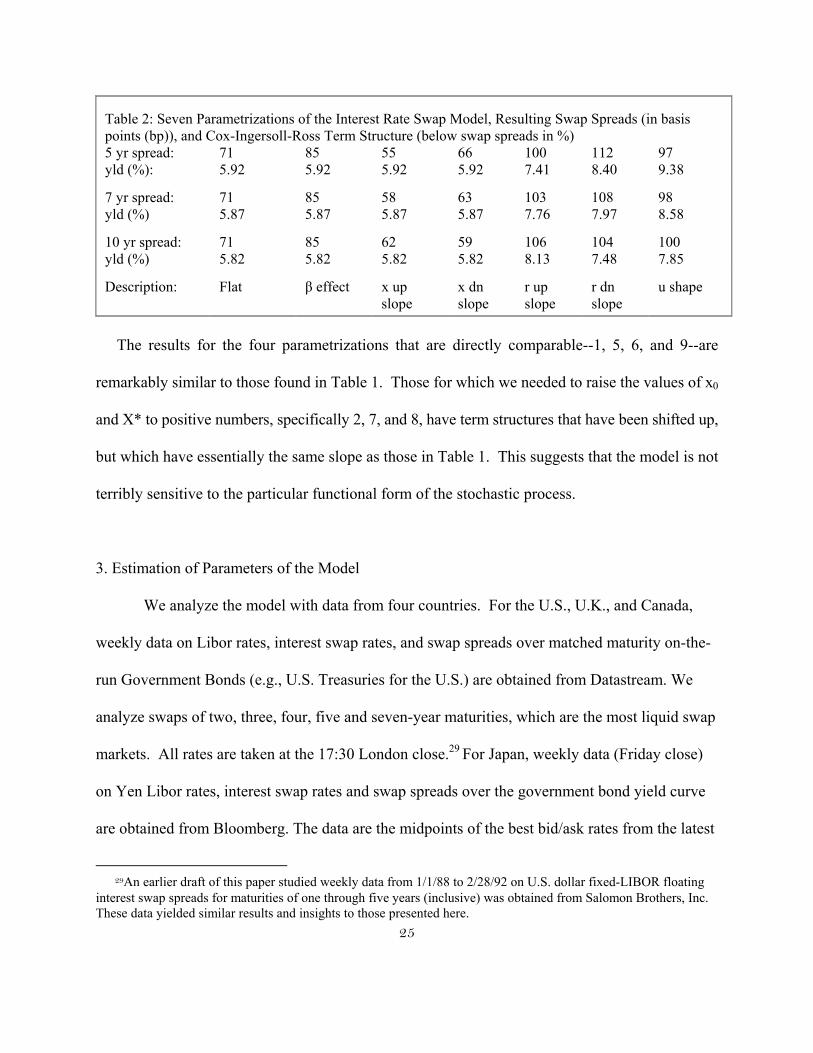
Table 2, using seven parametrizations, explores the effect of the CIR square root processes on

the interest rate swap spread. The parametrization numbers at the top of the table correspond to

those in Table 1. For comparison purposes, we use parameter values that are somewhat comparable

(in a risk-neutral pricing environment) to those used in Table 1. This is not possible for

parametrizations 3 and 4, which have a non-zero ρ, nor for parametrization 10, which has extreme

negative values of x0 and X*, which are not permitted in a square root process. For the two

parametrizations, 7 and 8, that have small, identical, negative values of x0 and X*, we use their

absolute values, .0025. We employ the same values for parametrization 2, which had zero values

24

for x0 and X*. The remaining four parametrizations, 1, 5, 6, and 9, essentially use the same

parameters as found in Table 1, with one caveat: In all seven parametrizations, the two volatility

parameters are not directly comparable between the Ornstein-Uhlenbeck model and the square root

model. To make the comparison as close as possible, we convert the Ornstein-Uhlenbeck σr and σx

into square root volatilities by dividing each respectively by the square roots of R* and X*, where

R* =κr*/(κ + λ) and X* = θx*/(θ+µ).

Table 2: Seven Parametrizations of the Interest Rate Swap Model, Resulting Swap Spreads (in basispoints (bp)), and Cox-Ingersoll-Ross Term Structure (below swap spreads in %)

Params 1 2 5 6 7 8 9

R* (%) 6 6 6 6 10 6 6

X* (bp) 70 25 80 40 25 25 100

r0 (%) 6 6 6 6 6 10 14

x0 (bp) 70 25 40 80 25 25 30

κ .2 .2 .2 .2 .2 .2 .4

θ .2 .2 .2 .2 .2 .2 .12

σr (%) (CIR) 8.165 8.165 8.165 8.165 8.165 8.165 8.165

σx (%) (CIR) 11.952 11.952 11.952 11.952 11.952 11.952 11.952

ρ 0 0 0 0 0 0 0

β 0 .1 0 0 .1 .1 .05

Swap Spreads and Term Structure

1 yr spread:yld %:

715.99

865.99

455.99

775.99

906.37

1249.62

10012.58


715.98

865.98

485.98

745.98

936.69

1219.26

9811.48


715.96

865.96

515.96

715.96

966.97

1178.95

9710.61


715.94

865.94

535.94

685.94

987.21

1158.66

979.92

25

Table 2: Seven Parametrizations of the Interest Rate Swap Model, Resulting Swap Spreads (in basispoints (bp)), and Cox-Ingersoll-Ross Term Structure (below swap spreads in %)5 yr spread:yld (%):

715.92

855.92

555.92

665.92

1007.41

1128.40

979.38

7 yr spread:yld (%)

715.87

855.87

585.87

635.87

1037.76

1087.97

988.58

10 yr spread:yld (%)

715.82

855.82

625.82

595.82

1068.13

1047.48

1007.85

Description: Flat β effect x upslope

x dnslope

r upslope

r dnslope

u shape

The results for the four parametrizations that are directly comparable--1, 5, 6, and 9--are

remarkably similar to those found in Table 1. Those for which we needed to raise the values of x0

and X* to positive numbers, specifically 2, 7, and 8, have term structures that have been shifted up,

but which have essentially the same slope as those in Table 1. This suggests that the model is not

terribly sensitive to the particular functional form of the stochastic process.

3. Estimation of Parameters of the Model

We analyze the model with data from four countries. For the U.S., U.K., and Canada,

weekly data on Libor rates, interest swap rates, and swap spreads over matched maturity on-the-

run Government Bonds (e.g., U.S. Treasuries for the U.S.) are obtained from Datastream. We

analyze swaps of two, three, four, five and seven-year maturities, which are the most liquid swap

markets. All rates are taken at the 17:30 London close.29 For Japan, weekly data (Friday close)

on Yen Libor rates, interest swap rates and swap spreads over the government bond yield curve

are obtained from Bloomberg. The data are the midpoints of the best bid/ask rates from the latest

29An earlier draft of this paper studied weekly data from 1/1/88 to 2/28/92 on U.S. dollar fixed-LIBOR floating

interest swap spreads for maturities of one through five years (inclusive) was obtained from Salomon Brothers, Inc. These data yielded similar results and insights to those presented here.

26

quoted rates collected by Bloomberg. For each security, we exclude weeks where any of the

data for a particular maturity are missing. The U.S. and Canadian data are from June 1, 1993 to

April 3, 2001 (410 weeks). The U.K. data are from September 8, 1998 to April 3, 2001 (135

weeks). The data from Japan are from January 15, 1999 to April 3, 2001 (108 weeks).

The payment frequency on the swap rates and spreads are semi-annual and the floating

leg is 6 month LIBOR in the relevant currency. The LIBOR day count convention is actual/360.

We adjust all rates to be semi-annually compounded rates for consistency.

In this section, we use this data to estimate the parameters of the general model assuming x

and r are independent. Recall from the discussion at the end of section 2.1 that when x and r are

independent and equation (11) describes the risk neutral stochastic process for x, the swap spread

for a swap of maturity T is

[ ] ,

iT/N) ,rP(T/N

dt )X - x(e + Xt) ,rP( + T)),rP( - (1 = Spread(T)Swap

0

N

=1i

*0

t -*0

T

00

*

∑

∫ θβ (21)

This encompasses both the CIR and Vasicek versions of the model, although the zero prices P(r0,

t) and the risk-neutral parameters, X* and θ* for a given X and θ would vary between the models.

Rather than second guess the functional form of the term structure, we use the actual term structure

to compute the zero coupon prices P(). Specifically, using data on 6 month and 1-year LIBOR, as

well as the 2,3,4, 5, and 7-year all-in-cost, we employ a cubic spline to interpolate the all-in-cost for

maturities 1.5, 2.5, 3.5, 4.5, 5.5, 6.0, and 6.5 years and then compute ten semi-annual zero coupon

bond prices from the all-in-cost rates. We then apply a second cubic spline to the semi-annual zero

coupon prices to obtain interpolated zero coupon prices for each interval of time necessary for the

27

numerical integration.30

Equation (21), the swap spread valuation equation, can be viewed as a fairly simple regression

that is nonlinear in only one parameter, θ* and, given θ*, for a time series of length τ, is linear in the

coefficients x0(1), ..., x0(τ), β, and X*. There is no constant in the regression. To estimate

parameters, we pool cross-section and time series and minimize the total sum of squares. For the

U.S. data, with 410 time series observations on five maturities, we have 2050 pooled observations

and 413 parameters to estimate.31 To obtain parameters that minimize the total sum of squares, we

first orthogonalize x and the term structure of interest rates (as represented by the LIBOR all-in-cost

curve), by regressing the pooled cross-section and time series of swap spreads on the all-in-cost of

the swap and a constant. The slope coefficient in this univariate regression is β. We then use the

intercept plus the residuals from this regression as dependent variables in a nonlinear multiple

regression.32 We first guess a value for θ* and then obtain OLS estimates of the remaining

parameters, x0(1),. . .,x0(τ), and X*.33 Iteration on θ* is guided by the Newton-Raphson

algorithm. Table 3 summarizes the parameter estimates for the four countries. Panels A through E

of Figure 3, each panel corresponding to a particular maturity, graph the actual and predicted values

for the swap spreads in each of the four countries through time.

30This numerical integration was performed with the routine provided with MATLAB.

31In general, with T times series observations and five maturities, there are 5T data points used to estimateT+3 parameters.

32The intercept in the second regression is suppressed.

33Since these coefficient estimates are linear functions of dependent variables that are constructed to beorthogonal to interest rates, we would expect them to be reasonably orthogonal to the r's that generate theinterest rates.

28

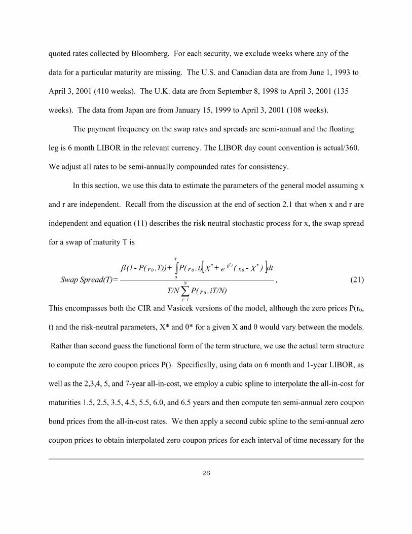
Table 3. Parameter Estimates and Standard Errors (in Parentheses) for the General Model

Parameters are obtained by minimizing the total sum of squared errors in Equation 21, using datafrom a pooled cross-section and time series. For a given θ*, OLS estimates of the remainingparameters are obtained in a two step regression--the first step a univariate regression of swapspreads on the all-in-cost and the second step a regression of residuals plus the constant from thefirst regression on the remaining variables in the swap spread equation. Iteration on θ* is guidedby the Newton-Raphson algorithm. Standard errors for X* are obtained assuming that θ* isestimated without error and using the OLS formulae for standard errors on the remainingcoefficients. Standard errors of the average x0 are computed as the standard error of the mean of thereproduced time series.

_______________________________________________________________________

The U.S. and Japan have mean reversion parameters that are positive but are rounded to zero.

This indicates that the component of the convenience yield that is unrelated to the level of interest

rates is virtually indistinguishable from a random walk.34 It is important to point out, however, that

the model is fit only with swap spread data and can therefore only determine the "risk-neutral"

parameters.

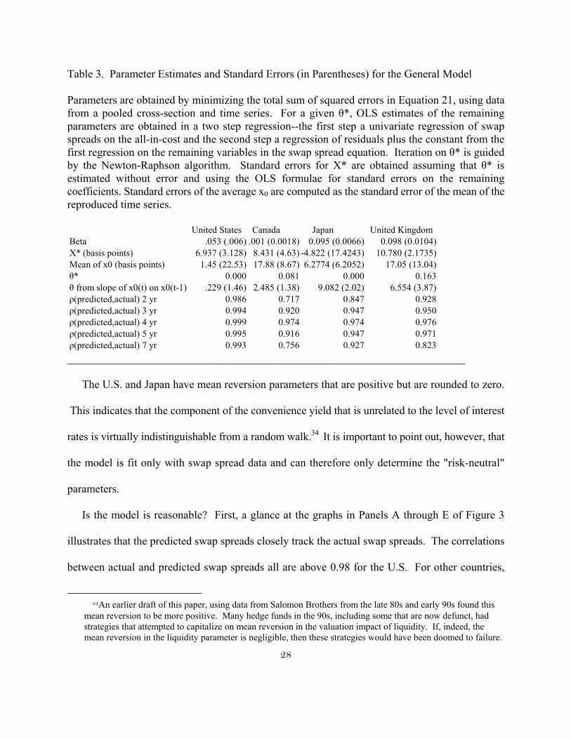
Is the model is reasonable? First, a glance at the graphs in Panels A through E of Figure 3

illustrates that the predicted swap spreads closely track the actual swap spreads. The correlations

between actual and predicted swap spreads all are above 0.98 for the U.S. For other countries,

34An earlier draft of this paper, using data from Salomon Brothers from the late 80s and early 90s found this

mean reversion to be more positive. Many hedge funds in the 90s, including some that are now defunct, hadstrategies that attempted to capitalize on mean reversion in the valuation impact of liquidity. If, indeed, themean reversion in the liquidity parameter is negligible, then these strategies would have been doomed to failure.

United States Canada Japan United KingdomBeta .053 (.006) .001 (0.0018) 0.095 (0.0066) 0.098 (0.0104)X* (basis points) 6.937 (3.128) 8.431 (4.63) -4.822 (17.4243) 10.780 (2.1735)Mean of x0 (basis points) 1.45 (22.53) 17.88 (8.67) 6.2774 (6.2052) 17.05 (13.04)θ* 0.000 0.081 0.000 0.163θ from slope of x0(t) on x0(t-1) .229 (1.46) 2.485 (1.38) 9.082 (2.02) 6.554 (3.87)ρ(predicted,actual) 2 yr 0.986 0.717 0.847 0.928ρ(predicted,actual) 3 yr 0.994 0.920 0.947 0.950ρ(predicted,actual) 4 yr 0.999 0.974 0.974 0.976ρ(predicted,actual) 5 yr 0.995 0.916 0.947 0.971ρ(predicted,actual) 7 yr 0.993 0.756 0.927 0.823

29

where the data may be less reliable, they range from 0.72 to 0.98. None of the parameter estimates

is of an unreasonable sign or magnitude. Finally, different ways of obtaining the same parameter

estimates yield similar results. For example, no constraints are placed on the estimation of x0's, (as

would be the case, for example, with Kalman filter estimation) other than that they fit the swap

spread data. However, if x follows an AR1 process, θ = θ*. A comparison of the mean reversion

parameter obtained from regressing the x0's on their lag1 values with the mean reversion parameter

that provides the best fit for the swap spreads indicates that, except for Japan, they are within two

standard errors of one another.35

4. Conclusion

This paper is a first attempt to develop a model where liquidity considerations alone generate

interest rate swap spreads. It may also be the first paper to value liquidity with the valuation

techniques developed for derivatives. For certain parameter restrictions, closed form solutions can

be found for a number of interest rate processes, including multifactor ones.

An alternative way to think about these issues is to note that we have implicitly added a factor

to traditional models of the government yield curve. The model starts with the yield curve generated

by the all-in-cost of the swap (also known as the LIBOR term structure). The government yield

curve is then derived from the LIBOR term structure by annuitizing the present value of a stochastic

liquidity factor (the swap spread) and subtracting it from the LIBOR term structure. Hence, a 1-

factor model of the yield curve can be thought of, not as a 1-factor model of the government yield

curve but as 1-factor model of the all-in-cost curve (the LIBOR yield curve). The government yield

30

curve is then generated by considering the effect of the additional liquidity factor.

The model can generate term structures for interest rate swap spreads that have a variety of

shapes, including U-shaped and humped curves. Elementary inspections of the swap spreads

generated by the estimated model indicate that it is adequate at explaining the existing empirical data

on swap spreads.

Interestingly, the model implies that the risk-free rate derived from government securities may

be inappropriate as implicit risk-free rates for models of the pricing of corporate securities.

Empirical analyses of U.S. data have long suggested that the implicit risk-free (or zero beta) rates

for popular risk return models of corporate securities, like the CAPM and APT, are substantially

higher than the government risk-free rate derived from Treasury Bills. A number closer to the

corporate risk free rate derived from LIBOR is also implicit in option prices. It is possible that the

failings of asset pricing models in this arena arise from the inappropriate use of the government risk-

free rate, which is lowered by the liquidity-based convenience yield, as parameters. A risk-free rate

that is close to short-term LIBOR, which this model suggests is the appropriate one to use for the

CAPM, APT, and Option Pricing Models, provides a far better empirical fit to historical data.

An issue that the model does not address is the effect of special repo. The model makes the

assumption that the liquidity advantage of government notes of all maturities is the same.

Realistically, differences in the liquidity-based convenience yield of the government notes, due to

some issues being "more special" than others at certain times needs to be accounted for. However,

a model where there are different liquidity-based state variables for different maturities is not

testable without further restrictions. One alternative is to keep the model in its current form and treat

35This is an overly conservative statement since the comparison assumes that θ* is estimated without error.

31

the effect of special repo as serially correlated measurement error in tests. This presents

identification problems of its own, in that it may be impossible to determine if the serial correlation

is driven by special repo or by some other misspecification of the model.

A potential limitation of the model is that the state variable for the liquidity-based convenience

yield is observationally equivalent to a state variable for credit risk. We circumvented this issue by

assuming that there is zero default risk of any type embedded in swap spreads. In practice, this

assumption may be a bit extreme. We know for example that a handful of corporations with the very

best credit rating borrow, short-term, at a few basis points below LIBOR. This would seem to

indicate that there is a small amount of compensation for default risk built into LIBOR. The thrust

of our argument, however, is that this is miniscule--at most on the order of 10% to 20% of the swap

spread. By far, the critical determinant of the swap spread is an amortized present value of a

liquidity-based convenience yield.

In principle, one could differentiate the miniscule default risk component of the swap spread

from the liquidity-based component by modeling the stochastic processes for these components

differently. However, there is little economic guidance for modeling a distinction between these

components. Moreover, such arbitrary distinctions in the modeling alone will dictate whether

empirical research finds that the swap spread is largely due to default risk or largely due to liquidity.

A better alternative is to test the model by supplementing the swap spread data with data on other

rates or spreads known to have differing default or liquidity properties. In addition to special repo

rates, as discussed above, general collateral repo rates, spreads between such rates and LIBOR, and

spreads between short-term borrowing rates of the most creditworthy corporations and LIBOR may

be useful. Such data were unavailable to us, but represent an interesting avenue for future research.

32

APPENDIX

Proof that

∫

κθθκσσρττ κθθ

+e - 1 - e - 1t),rP(- = x(t) ,e )dr(cov

)t+-(t-xr

0

t

0

-

.Define for all points in time τ

φ = eκτr.ψ = eθτx.

By Ito's Lemma

dφ = κeκτR*dt + eκτσrdz anddψ = θeθτX*dt + eθτσxdw,

By Stein's Lemma,

,),(- =

,

))]dz(ee)(dz(s)deeE[(trP

(t))e)d(et)cov(,rP(- =

x(t)) ,)dr(cov(e )dr(E- = x(t) ,e )dr(cov

x

t

0

t-r

s

0

-t

00

t--t

00

t

0

t

0

-

t

0

-

τσρτσ

ψττφ

ττττττ

θτθκτ

κτ

θκτ

∫∫∫

∫

∫∫∫

where s is a variable indexing time. Reversing the order of integration for the double (partially

stochastic) integral above,

33

,- =

-- =

)dee(eeP(t)-

))]dz(e))()dz(eee[(eP(t)-

))]dz(ee))()dz(de(eP(t)E[(- = x(t) ,e )dr(cov

-t-)+(t

0

xrt-

x

t

0

-t-rt

0

t-

x

t

0

t-r

-tt

0

t

0

-

E

τκσσρ

τσρτκσ

τρσττσττ

κτκτθκθ

θτκτκκτθ

θτθκτ

τ

κτ

∫

∫∫

∫∫∫∫

−

(

where the latter equality follows from the independence of the non-contemporaneous dz's and theBrownian motion assumption that E(dz2) = dτ. Completing the integration,

. +

e - 1 - e - 1-P(t)=

1 - e - e+1 - e-

eP(t)- = x(t) ,e )dr(cov

)t+-(t-xr

tt-

)t+(xrt-

t

0

-

∫

κθθκσσρ

θθκκσσρττ

κθθ

θκ

θκθ

34

References

Amihud, Yacov and Haim Mendelson, 1991, "Liquidity, Maturity, and the Yields on U.S.treasury Securities," Journal of Finance, 46, 1411-1425.

Boudoukh, Jacob and Robert Whitelaw, 1993, "Liquidity as a Choice Variable: A lesson fromthe Japanese Government Bond Market," Review of Financial Studies, 6 (2), 266-292.

Brennan, Michael, 1991, "The Price of Convenience and the Valuation of CommodityContingent Claims," in D. Lund and B. Øksendal (eds.), Stochastic Models and Option Values,Elsevier Science Publishers (North Holland).

Chen, Andrew and Arthur K. Selender, 1994, "Determination of Swap Spreads: An EmpiricalAnalysis," Southern Methodist University Working Paper.

Cooper, Ian and Antonio Mello, 1991, "The Default Risk of Swaps," Journal of Finance 46, 597-620.

Cox, John, Jonathan Ingersoll, and Stephen Ross, 1985, "A Theory of the Term Structure ofInterest Rates," Econometrica 53, 385-407.

Daves, Phillip and Michael Erhardt, 1993, "Liquidity, Reconstitution, and the Value of U.S.Treasury Strips," Journal of Finance, 48 (1), 315-330..

Duffie, Darrell, 1996, "Special Repo Rates," 1996, Journal of Finance, 51 (2), 493-526.

Duffie, Darrell and Ming Huang, 1996, “Swap rates and Credit Quality,” Journal of Finance, 51(3), 921-949.

Duffie, Darrell and Kenneth Singleton, 1997, “An Econometric Model of the Term Structure ofInterest-Rate Swap Yields,” Journal of Finance, 52 (4), 1287-1321.

Evans, E. and Giola Parente Bales, 1991, "What Drives Interest Rate Swap Spreads?" in InterestRate Swaps, Carl Beidleman, ed. 280-303.

Grinblatt, Mark and Francis Longstaff, 2000, “Financial Innovation and the Role of DerivativeSecurities: An Empirical Analysis of the Treasury Strips Program,” Journal of Finance 55 (3),1415-1436.

Jarrow, Robert and Fan Yu, 2001, “Counterparty Risk and the Pricing of Defaultable Securities,”Journal of Finance, 56 (5), 1765-1799.

Kamara, Avraham, 1994, "Liquidity, Taxes, and Short-Term Treasury Yields," Journal ofFinancial and Quantitative Analysis, 29(3), 403-417.

35

Litzenberger, Robert, 1992, "Swaps: Plain and Fanciful," The Journal of Finance, 597-620.

Longstaff, Francis and Eduardo Schwartz, 1995, "A Simple Approach to Valuing Risky Fixedand Floating Rate Debt," Journal of Finance, 50 (3), 789-819.

Minton, Bernadette, 1997, "An Empirical Examination of Basic Valuation Models for PlainVanilla U.S. Interest Rate Swaps," Journal of Financial Economics, 44 (2), 251-277.

Sarig, Oded and Arthur Warga, 1989, "Bond Price Data and Bond Market Liquidity," Journal ofFinancial and Quantitative Analysis, 24(3), 367-378.

Sun, Tong-Sheng, Suresh Sundaresan, and Ching Wang, 1993, "Interest Rate Swaps: AnEmpirical Investigation," Journal of Financial Economics, August, 77-99.

Sundaresan, Suresh, 1991, "Valuation of Swaps," in Recent Developments in InternationalBanking and Finance, S. Khoury, ed. Amsterdam: North Holland (Vols. IV and V, 1991).

Uhlenbeck, G.E. and L.S. Ornstein, 1930, "On the Theory of Brownian Motion," PhysicalReview 36, 823-841.

Vasicek, Oldrich, 1977, "An Equilibrium Characterization of the Term Structure," Journal ofFinancial Economics 5, 177-188.

Warga, Arthur, 1992, "Bond Returns, Liquidity, and Missing Data," Journal of Financial andQuantitative Analysis, 27(4), 605-617.

2

FIGURE 3: Panel AFitted and Actual Values for 2 Year Swap Spreads Over Time for 4 Countries

Two Year Swap Spread: United States

0

0.1

0.2

0.3

0.4

0.5

0.6

0.7

0.8

0.9

1

Jun-93 Jun-94 Jun-95 Jun-96 Jun-97 Jun-98 Jun-99 Jun-00

Date

Yie

ld(%

)

Market

Model

Two Year Swap Spread: Japan

-0.05

0

0.05

0.1

0.15

0.2

0.25

0.3

Jan-99 May-99 Sep-99 Jan-00 May-00 Sep-00 Jan-01

Date

Yie

ld(%

)Market

Model

Two Year Swap Spread: United Kingdom

0

0.2

0.4

0.6

0.8

1

1.2

Sep-98 Jan-99 May-99 Sep-99 Jan-00 May-00 Sep-00 Jan-01

Date

Yie

ld(%

)

Market

Model

Two Year Swap Spread: Canada

0

0.1

0.2

0.3

0.4

0.5

0.6

0.7

0.8

0.9

1


Date

Yie

ld(%

)

Market

Model

Figure 3Panel B: Fitted and Actual Values for 3 Year Swap Spreads Over Time for 4 Countries

Three Year Swap Spread: United States

0

0.2

0.4

0.6

0.8

1

1.2


Dat e

Mar ket

Model

Thre e Ye ar S wap S pre ad: Japan

0

0.05

0.1

0.15

0.2

0.25

0.3

0.35


D a t e

Mar ket

Model

Three Year Swap Spread: United Kingdom

0

0.2

0.4

0.6

0.8

1

1.2


Date

Yie

ld(%

)

Market

Model

Three Year Swap Spread: Canada

0

0.1

0.2

0.3

0.4

0.5

0.6

0.7


Date

Yie

ld(%

)

Market

Model

FIGURE 3Panel C: Fitted and Actual Values for 4 Year Swap Spreads Over Time for 4 Countries

Four Year Swap Spread: United States

0

0.2

0.4

0.6

0.8

1

1.2


Date

Yie

ld(%

)

Market

Model

Four Year Swap Spread: Japan

0

0.05

0.1

0.15

0.2

0.25

0.3

0.35


D a t e

Mar ket

Model

Fo ur Ye ar S wap S pre ad: Unite d Kingdo m

0

0.2

0.4

0.6

0.8

1

1.2


D a t e

Mar ket

Model

Four Year Swap Spread: Canada

0

0.1

0.2

0.3

0.4

0.5

0.6

0.7


Dat e

Mar ket

Model

FIGURE 3Panel D:Fitted and Actual Values for 5 Year Swap Spreads Over Time for 4 Countries

Five Year Swap Spread: United States

0

0.2

0.4

0.6

0.8

1

1.2


Date

Yie

ld(%

)

Market

Model

Five Year Swap Spread: Japan

0

0.05

0.1

0.15

0.2

0.25

0.3

0.35

0.4


Date

Yie

ld(%

)

Market

Model

Five Ye ar S wap S pre ad: Unite d Kingdo m

0

0.2

0.4

0.6

0.8

1

1.2

1.4


D a t e

Mar ket

Model

Five Year Swap Spread: Canada

0

0.1

0.2

0.3

0.4

0.5

0.6

0.7


Date

Yie

ld(%

)

Market

Model

FIGURE 3Panel E: Fitted and Actual Values for 7 Year Swap Spreads Over Time for 4 Countries

Seven Year Swap Spread: United States

0

0.2

0.4

0.6

0.8

1

1.2

1.4


Date

Yie

ld (%

)

Market

Model

Seven Year Swap Spread: Japan

0

0.05

0.1

0.15

0.2

0.25

0.3

0.35

0.4

0.45

0.5


Date

Yie

ld (%

)

Market

Model

Seven Year Swap Spread: United Kingdom

0

0.2

0.4

0.6

0.8

1

1.2

1.4


D a t e

Mar ket

Model

Seven Year Swap Spread: Canada

0

0.1

0.2

0.3

0.4

0.5

0.6

0.7

0.8


Dat e

Mar ket

Model

an analytic solution for interest rate...

Documents