an analytical model for a sequential investment opportunity · manchester business school ... an...

An Analytical Model for a Sequential Investment OpportunityRoger Adkins*

Bradford University School of Management

Dean Paxson**

Manchester Business School

January 15, 2014

JEL Classifications: D81, G31, H25

Keywords: Real Option Analysis, Multi-stage Multi-factor Sequential Investment, Perpetual

Compound Option, Catastrophic Risk

Acknowledgements: We thank Alcino Azevedo, Jörg Dockendorf, Michael Flanagan, Raquel

Gaspar, Kuno Huisman, Clara Raposo, Artur Rodriques, Mark Shackleton, Azfal Siddique,

Sigbjørn Sødal and participants at the Real Option Conferences, 2012 London, 2013 Tokyo, and

the ISEG Technical University of Lisbon Spring 2013 Seminar, for helpful comments on

previous versions.

*Bradford University School of Management, Emm Lane, Bradford BD9 4JL, UK.

[email protected]

+44 (0)1274233466.

**Manchester Business School, Booth St West, Manchester, M15 6PB, UK.

[email protected]

+44(0)1612756353. Corresponding author.

2

An Analytical Model for a Sequential Investment OpportunityAbstractWe provide a generalized analytical closed-form solution based on an American perpetual

compound option representation for a real sequential investment opportunity, which does not

rely on a multivariate distribution function. This model is especially applicable for R&D

projects, such as a drug development that requires investigation, testing, clinical trials and

production, where failure can occur at any stage. Other sources of uncertainty include the project

value and the investment cost at each stage. A feasible model solution entails both the stage

failure probability decreasing towards the completion stage and a lower bound on the

consecutive investment cost ratio. A project value volatility increase raises the option value at

each stage, as expected, and raises the project value threshold that justifies investment but only at

the completion stage. A similar pattern is observed for an investment cost volatility increase, as

well as for composite volatility increases arising from correlation changes. While the threshold

for completing a project is higher for increased volatility, it is lower for starting a project. A

reverse pattern is observed for the stage failure probability. While the threshold for completing

the project is lower for an increased probability, it is higher for the intermediate stages.

3

1 Introduction

We formulate the opportunity value for a project composed of multiple sequential investments as

a compound exchange perpetual American-style option. This extends the findings for a single

investment opportunity one-factor model, Tourinho (1979), and the two-factor model, McDonald

and Siegel (1986), to the case of multiple sequential investment opportunities. It also

complements the seminal work of Geske (1979) and Carr (1988) on European compound and

exchange options. The option value and project value thresholds are expressed as closed-form

solutions, which are free from onerous numerical calculations. But the solution depends on

assuming the possibility for a catastrophic failure at each investment stage with a probability that

declines as the project nears completion, which is a characteristic of many R&D, exploration and

infrastructure projects as well as initially many all-equity venture capital firms.

We conceive a real sequential investment opportunity as a set of distinct, ordered investments

that have to be made before the project can be completed. In this description, the project can be

interpreted as a collection of investment stages, such that no stage investment, except the first,

can be started until the preceding stage has been completed. Success at each stage is not

guaranteed because of the possibility of a catastrophic failure that reduces the option value to

zero. The project value is realized when all the stages have been successfully completed. The

following four-stage opportunity provides an illustration: (i) undertaking basic research. (ii)

developing a marketable product, (iii) testing its viability and (iv) implementing the

infrastructure for launch and delivery. Bearing in mind that a project can be composed of any

number of distinct stages, multiple sequential investment opportunities are common amongst

industries as diverse as oil exploration and mining, aircraft manufacture, pharmaceuticals and

consumer electronics. Schwartz and Moon (2000) illustrate a new drug development process

which consists of four distinct phases, each with a positive probability of failure, although not

necessarily declining over time. Cortazar et al. (2003) describe four natural resource exploration

stages of a project with technical success probability increasing over each phase, and then a

production phase which is subject to commodity price uncertainty. Pennings and Sereno (2011)

describe a typical development path of a new medicine over seven phases, with a probability of

failure declining over time.

4

Making an investment at a stage depends on whether the prevailing project value is of sufficient

magnitude to economically justify committing the prevailing investment cost, or whether it is

more desirable to wait for more favorable conditions. In our formulation, these two factors, the

project value and investment cost, are both treated as stochastic, and possibly correlated. After

making the stage investment, there is no absolute guarantee that the stage will be successfully

completed, because of the presence of irresolvable difficulties in converting intentions into

reality owing to technological, technical or market impediments. This suggests that the

investment opportunity at any stage is subject to a catastrophic failure that causes the option

value to be entirely destroyed, so the project as an entity becomes irredeemably lost. Our aim is

to analyze this sequential investment opportunity under the three sources of uncertainty, the

stochastic project value and the investment cost, which are permitted to be correlated, and the

probability of a catastrophic failure, so to be able to produce a closed-form rule on the

investment decision at each of the project stages. Because of value conservation, the option for

any stage except completion is evaluated at the point where the investment required to continue

is less than the value of the option created at the next stage. In this way, the sequential

opportunity is a compound option specified over multiple stages. We aim to formulate an

analytical solution to a multiple compound option based on American perpetuities.

In the absence of other forms of optionality, single-stage investment opportunity models based

on an American perpetuity option model yield a closed-form solution when the underlying

follows a geometric Brownian motion (gBm) process, Tourinho (1979) and McDonald and

Siegel (1986). However, this degree of analytical elegance has not yet been attained for the

multi-stage sequential investment opportunity. One of the first attempts to obtaining a solution

for sequential investments based on American perpetuity options is formulated by Dixit and

Pindyck (1994). They identify a rule for a two-stage sequential investment with fixed investment

costs, but their solution is seemingly implausible as it is identical to the one-stage result except

for the accumulated costs. Despite this setback, the sequential investment opportunity based on

American perpetuity options continues to remain an important problem to solve. The time

elapsed between stages may be unknown and uncertain rather than known and fixed, since

exercise is only warranted by a justifiable economic conditions rather than some fixed period of

5

time. Further, it is important to recognize that amongst other things, the project value may vary

between succeeding stages and the option value at each stage needs to be evaluated. To resolve

this dilemma, their formulation is recast by appealing to the time-to-build model of Majd and

Pindyck (1987). In this representation, firms can invest continuously, at a rate no greater than a

specified maximum, until the project has been completed, but investment may be temporarily

halted at any time and subsequently re-started, albeit at a zero cost. The solution, evaluated by

using numerical methods, shows the importance of the project value volatility in deciding

whether or not to suspend investment activities. Even though the investment levels can be

managed, it is essentially a single stage representation. The solution for an evaluation involving

costs as the only stochastic factor is presented by Pindyck (1993). Schwartz and Moon (2000)

extend their model by including the possibility of a catastrophic failure and the presence of

multiple stages, except that the solution is not analytical. Kort et al. (2010) propose that the

American perpetuity option value for a two-stage sequential investments is equal to the sum of

the separate option values, but this formulation suffers the defect of a lack of compoundedness in

the sense that the first and second stage option values are independent.

An alternative method for reaching a closed-form rule for sequential investment opportunities is

to suspend the need for an elapse time between stages that is unknown and uncertain, and to

replace it by one that is known and fixed. This relaxation converts the underlying option type

from American to European. The closed-form analytical formulation for evaluating a two-stage

sequential investment opportunity based on a European option, also known as a European-style

compound option, is originally derived by Geske (1979) for equity option valuation. By building

on the exchange option formulation of Margrabe (1978), Carr (1988) develops the N-stage

European compound exchange option, which can be applied to value multi-stage sequential

investment opportunities when both the project value and investment costs are stochastic.

Several authors adopt variations of the European-style compound exchange option framework

for investigating sequential investment opportunities. Two-stage formulations are proposed by

Bar-Ilan and Strange (1998), who suggest a quasi-analytical solution for stages having fixed,

known inter-stage durations and time to complete, with the possibility of infinite suspension in

the last stage, by Lee and Paxson (2001), who provide a numerical American-style option value

approximation for two stages, and by Paxson (2007) who provides an American-style

approximation with time to completion for two stages. A generalization to the N-stage compound

6

option is presented by Cassimon et al. (2004), which is used for investigating a new drug

application as a sequential investment opportunity. Other contributions include Agliardi and

Agliadi (2003) on generalizing the formula, Lee et al. (2008) on simulated sensitivities,

Cassimon et al. (2011) on phase specific volatility, and Ghosh and Troutt (2012) on software

solutions for multidimensional distributions, who also note that the calculation times for

5+stages solutions are lengthy.

N-stage European compound options with jumps are adopted by several authors for valuing

multi-stage sequential real investments: Brach and Paxson (2001) use a risk neutral approach

incorporating jumps for gene discovery and development; Cassimon et al. (2011) model a

pharmaceutical project with technical uncertainty, specified by a probability that deflates the

option value; Pennings and Sereno (2011) model a R&D project that allows for failure and

abandonment since technical uncertainty is represented as a Poisson jump process; and

Andergassen and Sereno (2012) analyze a R&D project as sequential compound exchange option

with a project value and investment costs following distinct gBm jump-diffusion processes.

Some authors eschew the reputed merits of closed-form European compound options and solve

the sequential investment opportunity through the power of numerical techniques. Cortelezzi

and Villani (2009) use Monte Carlo simulation for valuing a R&D project characterized as an

American sequential exchange option. A trinomial lattice formulation is used by Childs and

Triantis (1999) to solve a multiple sequential investment model having cash-flow interaction.

Koussis et al. (2013) provide numerical solutions for multi-stages with multiple options. The

shortcomings of these solution methods are the putative imprecision of the result as well as the

onerous calculations.

The aim of this paper is to reformulate and solve analytically the sequential investment model as

specified by Dixit and Pindyck (1994) by incorporating three distinct sources of uncertainty. The

three sources are characterized by the uncertainty associated with the project value and the

investment cost for each stage, and the possibility of a catastrophic failure that causes the

“sudden death” for the project. Based on American perpetuity option framework, we find that the

project value thresholds that activate exercise at each stage is a recursive expression represented

by a function of the investment cost threshold at the particular stage and those for all subsequent

stages. Further, similar to the European compound option model, Geske (1979), we demonstrate

7

that the option value for each stage is a homogenous degree-one and convex function, in keeping

with the Merton (1973) assertion. Amongst the three sources of uncertainty, the most crucial for

obtaining a meaningful solution is the possibility of catastrophic failure at each stage. Moreover,

we show that the existence of a meaningful solution demands that the probability of catastrophic

failure continually declines at all stages until the ultimate completion stage. Although the

presence of an uncertain investment cost is not critical to the solution development, its inclusion

does create a richer representation.

The major analytical findings for the sequential investment model are developed in Section 2.

Based on the three sources of uncertainty, the model is presented first for a one-stage

opportunity, and then incrementally developed for a two-, three- and finally N -stage sequential

investment opportunity. It is assumed that the failure probabilities at successive stages decline as

the stage nears completion. We develop closed-form solutions for whether or not to commit

investment at a particular stage and for the option value at each stage. In Section 3, we obtain

further insights into the behavior of the model through numerical illustrations. The last section

summarizes some advantages and limitations of our model and suggests plausible extensions.

2 Sequential Investment Model

A firm, which can be treated as being a monopolist in its market, is considering an investment

project made up of a discrete number of sequential stages, each involving an individual non-zero

investment cost. The project as an entity is not fully implemented and the project value not

realized until all of the sequential stages have been successfully completed. Each successive

investment stage relies on the successful completion of the investment made at the preceding

stage. We order each investment stage by the number J of remaining stages, including the

current one, until project completion. Although it may be more natural to label the initial stage of

the project as 1, a reverse ordering is used since a backwardation process is used in deriving the

solution. First, we examine the decision making position for the ultimate stage where 1J , and

then by replication, for the preceding stages, 2,3,J incrementally. At the ultimate stage, the

firm is considering the decision whether or not to make an investment in a real asset. This is

decided by whether or not the option value at 1J (“destroying the option value” by exercising

8

the investment) is compensated by the expected net present value of the cash flow stream due to

the investment. At the penultimate stage 2J , the firm is considering whether to make an

expenditure to obtain the investment option at 1J . This decision rests on whether or not the

option value at 2J fully compensates the net option value at 1J . This procedure is then

replicated incrementally for stages greater than 2. If the completion of any stage J occurs at time

JT , then 1J JT T for all positive integers J since the stages have to be completed

consecutively.

A representation of the sequential investments process for a J N stage project is illustrated in

Figure 1. This figure reveals the ordered sequence of stage investments comprising the project. It

also shows that after an investment, the possible outcomes are success and failure. If all the stage

outcomes are successful, then the entire project is successfully completed and its value can be

realized. However, there is a possibility of failure at each stage. Although the investment is

committed, the stage may not be successfully completed owing to fundamental irresolvable

technical or market impediments, in which case, the option value instantly falls to zero and the

project is abandoned without any value. The probability of failure at stage J is denoted by J

where 0 1J J . Situations do arise when an investment can produce an innovative

breakthrough and generate an unanticipated increase in the project value, but we have ignored

this possibility. Also, other forms of optionality, such as terminating a project before completion

for its abandonment value, are not considered.

---- Figure 1 about here ----

The value of the project is defined by V . This value cannot be realized until the ultimate

investment at 1J has been successfully completed. The investment expenditure made at any

stage J is denoted by JK for all possible values of J . Both the project value and the set of

9

investment expenditures are treated as stochastic. It is assumed that they are individually well

described by the geometric Brownian motion process1:

d d dX X XX X t X z , (1)

for , JX V K J , where X represent the respective drift parameters, X the respective

instantaneous volatility parameter, and d Xz the respective increment of a standard Wiener

process. Dependence between any two of the factors is represented by the covariance term; so,

for example, the covariance between the real asset value and the investment expenditure at stage

J is specified by:

Cov d ,d dJ JJ VK V KV K t .

Different stages may have different factor volatilities and correlations. The risk-free rate is r,

and the investment expenditure at each stage K is assumed to be instantaneous.

2.1 One-Stage Model

The stage 1J model represents the investment opportunity for developing a project value V

following the investment cost 1K , given that the research effort may fail totally with probability

1 . We only provide here the main results since the solution is directly obtainable from

McDonald and Siegel (1986). An alternative solution developed by Adkins and Paxson (2011)

and applied to the one-stage model is briefly described in Appendix A, since it naturally extends

to dimensions greater than two2.

The value 1F of the investment opportunity at stage 1J depends on the project value and the

investment cost, so 1 1 1,F F V K . By Ito’s lemma, the risk neutral valuation relationship is:

1 Other authors assume a mixed jump diffusion process for the underlying values, but in this case the entire project

fails, perhaps due to a collapse in the project value, or a significant escalation of the investment cost, or other

reasons, so the jump process is not confined to a particular element.2 The additional subscripts indicating the relevant quadrant are explained in Appendices A and B.

10

1 1

1

2 2 22 2 2 21 1 11 1

1 12 22 21 1

1 11 1 1

1

0

V VK V K

V K

F F FV K VKV K V K

F FV K r F ,V K

(2)

where the X for , JX V K J denote the respective risk neutral drift rate parameters. The

generic solution to (2) is the two-factor power function:

1 111 1 1 ,F AV K (3)

where 1 and 11 denote the generic unknown parameters for the two factors, project value and

investment cost, and 1A denotes a generic unknown coefficient. In this notation, the first

subscript for 1A , 1 and 11 refers to the specific stage under consideration, while the second

subscript of 10 refers to any feasible successive stage, which only becomes relevant for 1J .

By substituting (3) in (2), the power function satisfies the valuation relation with characteristic

root function:

1 1 1 1

1 1 11

2 21 11 1 11 11 1 11 1 11 12 21 1 0V K VK V K V K

Q ,

r .

(4)

Since a justified economic incentive to exercise the stage-one option exists provided that the

project value is sufficiently high and the investment cost is sufficiently low, and the incentive

intensifies for project value increases and investment cost decreases, we conjecture that

1 12 0 and 11 112 0 . Also 1 12 0A A since the option value is positive. Then (3)

becomes:

12 1121 12 1 .F A V K (5)

The threshold levels for the project value and the investment cost signaling the optimal exercise

for the investment option at stage 1J are denoted by 1V and 11K , respectively. The value

11

matching relationship describes the conservation equality at optimality that the option value

1 1 1 11ˆ ˆ ˆ,F F V K exactly compensates the net asset value 1 11

ˆ ˆV K . Then:

12 11212 1 11 1 11

ˆ ˆ ˆ ˆA V K V K . (6)

The first order condition for optimality is characterized by the two associated smooth pasting

conditions, one for each factor, Samuelson (1965). These can be expressed as:

12 112 1 1112 1 11

12 102

ˆ ˆˆ ˆ V KA V K

. (7)

Since the option value is always non-negative, 12 0A . Also, (7) corroborates our conjecture that

12 0 and 112 0 . Together, (6) and (7) demonstrate Euler’s result on homogeneity degree-

one functions, Sydsæter and Hammond (2006), so 12 112 1 . Replacing 112 by 121 in (4)

yields:

1 1

211 12 12 1 12 12 12 121 1 0 V K KQ , r , (8)

where1 1 1

2 2 21 2 V K V,K V K . From (8), 12 is obtained as the positive root solution for

the quadratic characteristic equation, which is greater than 1. Further, the threshold levels are

related by:

121 11

12

ˆ ˆ ,1

V K

(9)

with 12121

12 12 12 1A .

Applying Ito’s lemma to (5):

1 1 11 1 1d d d ,F F FF F t F z (10)

where

12

1 1 1 1 1

2 2112 12 12 122 1 2 1 ,F V K VK V K V K

1 1 1 1

22 2 2 212 12 12 121 2 1 .F V K VK V K

Under risk neutrality, the expected return on the option equals the risk-free rate adjusted by the

probability of failure, so1 1F r , which is borne out by 1Q , (8).

2.2 Two-Stage Model

At the preceding stage, 2J , the firm examines the viability of committing an investment 2K

to acquire the option to invest 1F by comparing the value of the compound option 2F with the

net benefits 1 2F K . Because of (3), 2F depends on the three factors V , 1K and 2K , so

2 2 1 2, ,F F V K K . By Ito’s lemma, the risk neutral valuation relationship for 2F is:

1 2

1 1 2 2 1 2 1 2

2 1

2 2 22 2 2 2 2 22 2 21 1 1

1 22 2 22 2 21 2

2 2 22 2 2

, 1 , 2 , 1 21 2 1 2

2 2 22 1 2 2

2 1

0.

V K K

V K V K V K V K K K K K

V K K

F F FV K KV K K

F F FVK VK K KV K V K K K

F F FV K K r FV K K

(11)

We conjecture that the solution to (11) is a product power function, with generic form:

24 21 222 2 1 2 ,F A V K K (12)

where 2 , 21 and 22 denote the generic unknown parameters for the three factors, project

value and investment expenditure at stage one and two respectively, and 2A denotes an

unknown coefficient. Substitution reveals that (12) satisfies (11), with characteristic root

equation:

13

1 2

1 1 2 2 1 2 1 2

1 2

2 2 21 22

2 2 21 1 12 2 21 21 22 222 2 2

2 21 2 22 21 22

2 21 22 2

, ,

1 1 1

0.

V K K

VK V K VK V K K K K K

V K K

Q

r

(13)

Since the stage-two option value increases for positive changes in 2V but for negative changes in

12K and 22K , we conjecture in Appendix B that the relevant hyper-quadrant is labeled IV where

2 24 0 , 21 214 0 and 22 224 0 . From (12), the option valuation function

becomes:

24 214 2242 24 1 2F A V K K . (14)

We specify that the stage-two threshold levels signaling an optimal exercise are represented by

2V , 21K and 22K for V , 1K and 2K , respectively. The set 2 21 22ˆ ˆ ˆ, ,V K K forms the boundary that

discriminates between the “exercise” decision and the “wait” decision. This boundary is

determined from establishing the relationship amongst 2V , 21K and 22K , or alternatively, from

identifying the dependence of 2V with respect to 21K and 22K . A stage-two option exercise

occurs for the balance between the stage-two option value 24 214 22424 2 21 22

ˆ ˆ ˆA V K K and the stage-one

option value 12 1112 1 11

ˆ ˆA V K less the investment cost 22K incurred in its acquisition. This equilibrium

amongst the threshold levels is the value matching relation that is expressed as:

24 214 224 12 12124 2 12 22 12 2 12 22

ˆ ˆ ˆ ˆ ˆ ˆ ,A V K K A V K K (15)

where 12A and 12 are known from the evaluation for stage-one. The three smooth pasting

conditions associated with (15), one for each of the three factors V , 1K and 2K , respectively,

can be expressed as:

24 214 224 12 12124 24 2 12 22 12 12 2 12

ˆ ˆ ˆ ˆ ˆ ,A V K K A V K (16)

24 214 224 12 121214 24 2 12 22 12 12 2 12

ˆ ˆ ˆ ˆ ˆ1 ,A V K K A V K (17)

14

24 214 224224 24 2 12 22 22

ˆ ˆ ˆ ˆ .A V K K K (18)

Since an option value is non-negative, then 24 0A . This implies that 24 0 from (16),

214 0 from (17), and 224 0 from (18), which justifies our conjecture on the signs of the

power parameters. Moreover, the dependence amongst the parameters can be found from

combining the smooth pasting conditions and the value matching relationship. First, the

comparison of (16) and (18) with (15) yields:

24224

12

1 ,

(19)

which implies that 24 12 . Second, the comparison of (18) with (19) yields:

12214 24

12

1 .

(20)

Third, a comparison of (19) with (20) yields:

24 214 224 1. (21)

The pattern amongst the parameters is highly significant. First, it leads to a simplification in

calculating their solution values. If we specify 24 24 12/ 0 , then by using the substitutions

24 24 12 , 214 12 241 and 224 241 , the quadratic function 2Q (13) can be expressed

as:

1 1 2

2

2 12 24 12 24 24

2 21 124 24 2 24 12 12 1 122 2

2

, 1 ,1

1 1

0,

V K K K

K

Q

r

(22)

where

1 2

1 1 2 2 1 2 1 2

22 2 2 2 22 12 12

12 12 12 12

1

2 1 2 2 1V K K

VK V K VK V K K K K K .

15

The value of 24 is evaluated as the positive root of 2 0Q , (22), where 12 is the previously

calculated stage-one solution. The values of 24 , 214 and 224 are then obtained from 24 and

12 . Subsequently, we show that 24 is greater than 1, so 24 12 .

The second significant feature is the ease in deriving the solution. Although the solution for 24A

and 2V as a function of 21K and 22K can be derived from the value matching relationship and the

smooth pasting conditions, (15) - (18), a more convenient way is based on the homogeneity

degree-one property for 2F , since the result is easily extendable for deriving the stage-three

solution and beyond. The valuation function 2F (12) can be expressed in the form:

22 2 1 11 21 12 22 1 2 2 1 1 2 2 1 1 2, , ,F F F K B F V K K B AV K K

(23)

where 22 2 1B A A . In this formulation, the two-stage option value 2F is a function 22 .F of two

stochastic factors: (i) the stage-one option value 1F (10), and (ii) the stage-two investment cost

2K . Moreover, since 2F is characterized as homogenous degree-one and its form (23) exactly

mirrors the stage-one investment option value 1F (3), the solution is directly obtainable from the

results for the one-stage model. If the stage-two thresholds for optimal exercise occur at the

levels 12 1 2 12ˆ ˆ ˆF F V ,K and 22K , for the stage-one option and the stage-two investment cost,

respectively, then the stage-two value matching relationship (15) can be expressed as:

24 24124 12 22 12 22

ˆ ˆ ˆ ˆ .B F K F K (24)

Except for the change in variable, (24) is identical in form to (6), so 24 241

24 24 241 /B ,

which implies:

2424 12

24 12

1 124 12

2424 12

1 1A

, (25)

16

so the two-stage option value is defined by:

24

24 12

12 2412 24 24

24 12

1 1124 12 1

2 2 1 2 2 1 224 12

1 1, ,F V K K V K K

. (26)

Also:

12 121 2412 1 2 12 12 2 12 22

24

ˆ ˆ ˆ ˆ ˆ,1

F F V K A V K K

, (27)

so:

1212

12 12

11 1

24 12122 12 22

12 24

1ˆ ˆ ˆ .1 1

V K K

(28)

For an economically meaningful solution to emerge, then from (27) 24 has to exceed one. In

(28), the threshold level for the stage-two project value 2V is related to the stage-one and stage-

two investment cost levels, 12K and 22K , respectively, and this relationship defines two-stage

compound option and extends the single stage standard result. The two investment cost threshold

levels enter the formulation as a weighted geometric average with weights dependent on only the

stage-one parameters. If the levels are specified to be equal, then the stage-two project value

level 2V and the equal investment cost level are linearly related, just as for 1V and 1K at stage-

one. The composite term:

12

1

24 1212

12 24

11 1

represents a stage-two variant mark-up factor. It is composed of two components: the stage-one

mark-up factor adjusted by a term reflecting the impact of the second stage. Since 12 24, 1 ,

the adjusting component 12

1

24 12 241 1 is greater than one provided 12 24(2 1 ) ,

which is always true for 12 24 . The variant mark-up factor can only be interpreted as to what

is generally understood to be a mark-up factor provided the two investment thresholds are equal,

17

for, if 12 22ˆ ˆK K , then 2 22

ˆ ˆV K equals the variant mark-up factor. Otherwise, the variant mark-up

factor measures the project value ratio relative to a weighted geometric average of the two

investment cost thresholds.

Standard real-option theory tells us that the underlying volatility has a profound effect on the

solution, McDonald and Siegel (1986), Dixit and Pindyck (1994). For a given value of the stage-

one power parameter 12 , a positive change in 2 produces a decrease in the parameter 24 , but

an increase in 24 24 1/ and in the adjusting component that yields an increase in the stage-

two mark-up factor. Now, the variance term 2 depends on the parameter 12 as well as the

volatilities for V , 1K and 2K , and their covariances. We first consider the consequences if all

the covariances can be assumed to be zero. High values for 12 , which are caused by low V

and1K , tend to ratchet up the value of 2 , while a value of 12 closer to 1 due to high V or

1K , tends to diminish the effect of1K in explaining 2 . The importance of

1K in determining

2 depends on its magnitude relative to V . Further, since the value of 12 depends positively

on the probability of a catastrophic failure at the 1J stage, the importance of2K relative to

V and1K in explaining 2 diminishes as the failure probability increases. It is through this

mechanism that the probability of catastrophic failure at stage one is translated into the

investment strategy at stage-two.

We now turn our attention to the effects of the covariance terms on 2 . If1

0VK ,2

0VK , or

1 20K K , then the value of 2 declines while the value of 12 increases relative to the instance

of zero correlations. This can be explained in the following way. A long investment cost acts as a

partial hedge for a long project value whenever1

0VK and2

0VK , since a random positive

(negative) movement in the investment cost is partly compensated by a movement in the same

direction in the project value. (A long/short position in the investment cost might be established

through fixed-price/cost-plus construction contracts). This partial hedge reduces the riskiness of

18

the combined position, which is reflected in a lower value of 2 . In contrast, a long investment

cost and V position becomes more risky whenever1VK or

2VK is negative. If1 2

0K K , then a

random movement in the 2J stage investment cost tends to be followed by a movement in the

opposite direction in the 1J stage investment cost, and a long 2J stage investment cost acts

as a hedge against a short 1J stage investment cost. A positive movement in the 2J stage

investment cost that is followed by a negative movement in the 1J stage investment cost can

be interpreted as dynamic learning, since a higher than anticipated preliminary investment cost

leads to a lower investment cost at a subsequent stage, while a negative movement in the 2J

stage investment cost that is followed by a positive movement in the 1J stage investment cost

can be interpreted as compensatory. Under-investment is corrected by over-investment at a

subsequent stage. In contrast, when1 2

0K K , the volatility 2 is inflated. This can arise from a

positive movement in the 2J stage investment cost that is followed by a positive movement in

the 1J stage investment cost, which suggests that errors at the earlier 2J stage are

compounded at the later 1J stage. However, a positive value for1 2K K can just as well be due

to a negative movement in the 2J stage investment cost followed by a negative movement in

the 1J stage investment cost. This may also represent bad news if low investment levels

presage low project values. Clearly, the sensitivity of the volatility 2 depends on the

magnitudes of the contributory quantities as well as their interactions.

By combining (22) with (8) in order to eliminate 12 , the 2Q function can be expressed as:

2 2

212 24 24 2 24 1 22 1 0.K KQ r r (29)

The parameter 24 , which is required to be greater than one, is evaluated as the positive root of

the quadratic function 2Q (29). Given that 22 0 , since it is a variance expression, then 24 1

provided that the value of 2Q evaluated at 24 1 is negative, Dixit and Pindyck (1994). It can

be observed from (29) that for 2 0Q at 24 1 , then 2 1 , see also Figure 2.

---- Figure 2 about here ---

19

The parameter measures the conditional probability of a catastrophic failure at a particular

stage. The existence of a solution to the sequential investment model represented by an

American perpetual compound option depends crucially on the probabilities at the two stages

following a distinct pattern. Although it plays an important role in deciding an acceptable

investment level at each stage, the stochastic nature of the investment expenditures is not critical.

The condition 2 1 for obtaining a meaningful solution continues to hold even if both1K and

2K are zero, so our findings also apply for a deterministic investment cost. The only

requirement for a meaningful solution to exist is that the conditional probability of a failure at the

2J stage has to exceed that for the 1J stage. This condition can be seen simply as a

stipulation imposed by the model structure. Since 2 2 11 , the failure probability at the

2J stage is always greater than that for the 1J stage. Alternatively, this condition could be

interpreted as the presence of dynamic learning. Because of the reduction in the failure

probabilities, the effect of making an investment at the 2J stage is to increase the affordable

amount of investment expenditure made at the subsequent stage. Ceteris paribus, project viability

is able to support a higher level of investment expenditure at the next stage, and this implies

some element of learning.

Model failure in the sequential investment formulation of Dixit and Pindyck (1994) is caused

owing to the project value thresholds triggering investment at the two sequential stages having

the same value. Because of this condition, the two sequential stages collapse to a single stage.

For the current model, we also need to investigate the nature of any conditions capable of

producing a similar collapse of the two sequential stages. This collapse would happen whenever

the project threshold at stage-two 2V equals or exceeds that at stage-one 1V , 2 1ˆ ˆV V , since under

the American perpetuity option representation, this would imply that an investment commitment

at stage-two triggers an investment commitment at stage-one. The relative magnitude of 1V and

2V is determined from comparing (9) and (28):

20

12

1

24 122 2

241 1

ˆ ˆ1ˆ ˆ1

V KV K

,

where 1 11 12ˆ ˆ ˆK K K and 2 22

ˆ ˆK K . Since 12 1 , then 2 1ˆ ˆV V if:

24 121

242

ˆ 11ˆ 1

KK

.

A meaningful solution exists provided that the ratio of the investment cost thresholds for stages-

one and –two exceeds the lower bound 2 24 12 241 1LB . This lower bound depends on

the parameter values for the relevant stochastic factors at the two stages, the probabilities of

stage failure, 1 and 2 , and the risk-free rate.

2.3 Three-Stage Model

Since the extension of the sequential investment model to the 3J stage is achieved by

replication, we only provide the crucial results with only a basic explanation. Then, the

comparison of the results for each of the three stages facilitates the formulation of a more general

result for a J N stage project.

The value of the option to invest at the 3J stage 3F depends on the project value V , and the

investment costs at the 1J , 2J and 3J stages, 1K , 2K and 3K , respectively, so

3 3 1 2 3F F V ,K ,K ,K . Using Ito’s lemma, it can be shown that the risk neutral valuation

relationship for 3F is a four-dimensional partial differential equation, whose solution is the

product power function:

3 13 23 333 3 1 2 3F A V K K K , (30)

with characteristic root equation:

21

1 2 3

1 1 2 2 3 3

1 2 1 2 1 3 1 3 2 3 2 3

1 2 3

3 3 13 23 33

2 2 2 21 1 1 13 3 13 13 23 23 33 332 2 2 2

3 13 3 23 3 33

13 23 13 33 23 33

3 13 23 33

1 1 1 1V K K K

VK V K VK V K VK V K

K K K K K K K K K K K K

V K K K

Q , , ,

r

3 0.

(31)

The function 3Q specifies a hyper-ellipse that has a presence in all possible quadrants. The

relevant quadrant is where 3 0 , 13 0 , 23 0 and 33 0 , since we expect the stage-three

investment option to become more valuable and its value to rise because of a project value

increase but an investment cost decrease. For convenience, we suppress the subscript

designating the relevant quadrant.

Alternatively, the valuation function 3F can be expressed as:

3 313 33 2 3 3 2 1 2 3, , , ,F F F K B F V K K K

(32)

where 3 3 2 3 2 1 , 13 3 12 3 2 11 , 23 3 22 3 21 , and 33 31 ,

with 1 1. The coefficient 3B is determined as:

3

3

3

33 3 2

3 3

111

B A A

At the stage-three investment decision, the thresholds signaling an optimal exercise for the stage-

three option value 3F , the stage-two option value 2F and the stage-three investment cost 3K are

denoted by 3 13 23 333 3 3 13 23 33

ˆ ˆ ˆ ˆ ˆF A V K K K , 23 2 3 13 23ˆ ˆ ˆ ˆF F V ,K ,K and 33K , respectively. Value

conservation at the stage-three investment holds when the stage-three option value 3F exactly

compensates the stage-two option value 23F less the investment cost 33K . The value matching

relationship becomes:

22

3 313 3 23 33 23 33

ˆ ˆ ˆ ˆF B F K F K . (33)

The optimal stage-three investment solution is obtained from the two smooth pasting conditions

associated with the value matching relationship (33) and can be expressed as:

323 33

3 1ˆ ˆF K

. (34)

Since from (26):

2

2 1

1 21 2 24

2 1

1 112 1 1

23 2 3 13 23 3 13 232 1

1 1ˆ ˆ ˆ ˆ ˆ ˆ ˆF F V ,K ,K V K K ,

(35)

then from (34):

1 22

2 11 1 2 1 2 1 2

12

1

1 1 13 2 13 13 23 3311

3 121 11

ˆ ˆ ˆ ˆV K K K

(36)

Clearly, an economically meaningful solution is only obtainable provided 3 exceeds 1, which

implies that 3 2 . If the investment cost threshold levels for the three stages are all equal,

then the project value threshold is a linear relationship of this equal investment cost threshold.

The stage-three mark-up factor in (36) can be expressed as:

1 1 21

1

1 1

32 121

2 31

11 11

where the first term is the stage-two mark-up factor and the second term 1 212 3 31 1

denotes the adjusting component. The stage-three mark-up factor exceeds the stage-two mark-up

factor provided 2 3 31 1 1 or 2 32 1 , which is true for 2 3 .

23

The existence of a meaningful solution to the current formulation requires that the stage-three

investment cost threshold level is less than that for stage-two. By comparing (28) with (36), we

have:

1 21

3 23 3

32 2

11

ˆ ˆV Kˆ ˆV K

, (37)

where 23 2ˆ ˆK K and 3 33

ˆ ˆK K . Similarly, for 3 2ˆ ˆV V , then the ratio of investment cost thresholds

2 3ˆ ˆK K has to be greater than the lower bound 3 3 2 31 1LB .

In (36), the solution to the boundary discriminating between investing and not investing at stage-

three requires evaluating only 3 , since 2 and 1 are presumed to have been calculated at each

of the subsequent two stages. By eliminating 13 , 23 and 33 from (31) yields after some

simplification:

1 2 3

3

3 3 2 1 3 2 1 3 2 3

213 3 32

2 21 13 2 2 2 2 1 1 1 1 1 22 2

3

1 1 1

1

1 1 1 1

0

V K K K

K

Q , , ,

r ,

where:

1 2 3

1 1 2 2 3 3

1 2 1 2 1 3 1 3 2 3 2 3

2 22 2 2 2 2 2 2 21 1 1 1 13 2 1 2 1 22 2 2 2 2

21 1 2 1 2 2 3 23 1 2

1 2 2 1 2 2

1 1

1 1

1 1 1 1

V K K K

VK V K VK V K VK V K

K K K K K K K K K K K K .

Then after further simplification, we obtain:

3 3

213 3 3 3 3 2 32 1 0K KQ r r . (38)

24

The value of 3 is the positive root solution to (38). By applying a similar argument as before, its

value exceeds one provided that 3 2 . Further, it depends not only on the stage-three

catastrophic failure probability 3 but also the probability 2 at the next stage, as well as on the

composite variance term 23 . This variance term is defined as the sum of variance and

covariances amongst the factors, the project value and the stage-three, -two and -one investment

costs, weighted by combinations of 3 , 2 and 1 . Because of this, the stage-three investment

commitment is decided by the properties of both the current and subsequent stages.

2.4 N-Stage Model

The solution to the 1J N stage of the sequential investment model is derived from the

results for the 2J and 3J stages by induction. The value of the option to invest at the

J N stage, denoted by 1N N NF F V ,K , ,K , is described by a 1N dimensional partial

differential equation, whose solution takes the form of a recursive product power function:

1 2 11 2 1

N N N NN N NN N N N N NF A V K K K B F K

, (39)

where the power parameters for NF are related to the J according to:

1 3 2 1 1

1 1 3 2 1 1 1

2 1 3 2 2 1

3 1 4 3 3 1

1 1 1 1

1

1

1

1

1

N N N N N

N N N N N

N N N N N

N N N N N

N N N N N N N

NN N

,,

,

,

,

.

(40)

Due to the homogeneity degree-one property, 1 2 1N N N NN . By inspection, we

observe from (40) that while N is positive, the JN for all J are negative. This means that the

investment option NF rises in value for increases in the project value but for decreases in the

investment cost at any of the stages.

25

The stage- N value matching relationship can now be defined as:

11 1

N NN N ,N NN N ,N NN

ˆ ˆ ˆ ˆB F K F K (41)

where 1ˆ ˆ ˆ, , ,N N NNV K K denote the respective optimal threshold levels with

1 1 1 2 1 1 1

1 1 1 1

1 1 2 1N N N N N

N ,N N N N N N

N N N N N N

ˆ ˆ ˆ ˆF F V ,K , ,K

ˆ ˆ ˆ ˆA V K K K .

The stage- N value matching relationship (41) is expressed in the form of a two factor

investment opportunity model, the value gained after exercise 1N ,NF and the investment cost

NNK , so the thresholds can be determined from standard theoretical results. It follows that:

1 1 1 2 1 1 11 1 1 2 1 1

N N N N N NN ,N N N N N N N NN

N

ˆ ˆ ˆ ˆ ˆ ˆF A V K K K K

, (42)

so:

1 2 11 2 1

N N N N NNN N N N N N NN

ˆ ˆ ˆ ˆ ˆV U K K K K . (43)

In (43), the parameters 0 1 2N N N NN, , , , are determined directly from (42):

0 1 1 3 2 1

1 1 1 1 1 1

2 2 1 1 2 2 1

3 3 1 1 3 3 2 1

1 1 1 1 1 1 3 2 1

1 1 3 2 1

1 1

1

1

1

1

1 1

N N N

N N N

N N N

N N N

N N N N N N N

NN N N

,,

,

,

,.

(44)

For 1, 2, ,J N , the JN are all positive since all the 1J , and 1 2 1N N NN owing

to the homogeneity degree-one property. This implies than an increase in any of the investment

26

cost threshold levels ˆJNK produces an increase in the project value threshold, and for any

particular J the elasticity of change is the positive constant 1JN . This means that higher

levels of the investment cost have to be compensated by higher project values. By inspection, we

also observe from (44) that:

12 13 14 23 24 25, ,

11 12 22 22 23 33, ,

or more generally

1 1 1

are equal for any and 1, 2, ,and for 2.

JN

NN NN N N

J N J JN

(45)

The coefficient NU , defined by:

0

1 1

N

NN

N N

UA

(46)

is the N -stage variant mark-up factor.

A meaningful solution to the sequential investment formulation exists provided that the project

value threshold for stage N is less than that for stage 1N . Because of (45) and (46), the ratio

of the project value thresholds from (43) is:

1 2 11

1

1 1

ˆ ˆ1ˆ ˆ1

N

N NN N

NN N

V KV K

, (47)

where ˆ ˆJN NK K for all J and N . Since 1 2 1 1N , then 1

ˆ ˆN NV V if the ratio of

investment cost thresholds 1ˆ ˆ

N NK K is greater than the lower bound:

1 1 1 .N N N NLB (48)

27

The parameter N is evaluated as the positive root of the quadratic characteristic root equation,

which can be expressed as:

2112 1 0

N NN N N N N N N K N KQ r r . (49)

In (49), the stage variance 2N is given by:

2 Tw ΩwN (50)

where Ω is the 1N dimensional square variance-covariance matrix with its first diagonal

element being 2V , the second

1

2K , and so on until 2

NK . The full expression is shown in

Appendix C. The off-diagonal elements denote the corresponding covariances. The column

vector w is given by:

1 3 2 1

1 3 2 1

1 3 2

1 2

1

1

1w

1

11

N

N

N

N N

N

Because of the homogeneity degree-one property, we have Tw 0i where i is the unit vector.

Note that for 1N , Tw 1 1 , .

Having evaluated N , we can solve for:

11 N

N

NN

N

B

, (51)

28

and then NA is determined from:

1N

N N NA B A . (52)

The 1, ,NA A and 1, ,NB B are obtainable from (51) and (52), recursively, starting from 1J

to J N . When 1J , 0A is treated as equaling 1.

Finally, the stage N option value is given by:

11

1 1

2 1 1 2

3 2 32

1 2 12

11

N NN N N N

N N N N

N N N N NN

N N J N NJ N

N

JJN

JJ

ˆB F K for V V ,ˆ ˆF K for V V V ,

ˆ ˆF K K for V V V ,

ˆ ˆF F K for V V V ,

ˆ ˆF K for for V V V ,

ˆV K for V V ,

(53)

assuming that 1 2 2 1N N Nˆ ˆ ˆ ˆ ˆV V V V V . Under this condition, if JV V then V in the stages

numbered , ,J N are above or at the threshold and are exercised, while those numbered

1, , 1J are below the threshold and remain unexercised. Clearly if 1V V then all the stages

are exercised. The below threshold option values can alternatively be found from (39).

The solution to the stage-N investment decision is obtained through a process of backwardation,

starting from the stage-one decision. This backwardation process yields consecutively the values

of 1 2 1N, , , , 1 2 1NB ,B , ,B and 1 2 1NA ,A , ,A , which are required for evaluating N , NB

and NA . From these values, we can then determine the discriminatory boundary linking the

29

project value threshold NV with the investment cost thresholds 1 2ˆ ˆ ˆ, ,N N NNK K K . Further, for a

meaningful solution to the stage-N investment decision to be obtained, the 1 2 1N N, , , , have

to individually exceed 1, which demands because of (49) that 1 2 1N N .

2.5 Analytical Characteristics

According to the two theorems of Merton (1973), options are homogenous degree-one in the

underlying and the exercise price, and options are convex in the underlying. In our analysis, the

underlying is represented by the project and the exercise price by the investment cost. It is

straightforward to show from (39) that the American perpetuity N -stage option value NF is

homogenous degree-one in the project value V and the set of relevant investment costs

1, ,NK K , since1

1N

N INI

. Because of this property, Euler’s theorem applies:

1

NN N

N II I

F FF V KV K

which is also a direct consequence of the sum of smooth-pasting conditions. Further, the N -

stage option value NF is homogenous degree-one in the 1N -stage option value 1NF and the

relevant investment cost NK , which implies that scaling has no material effect on the option

value, or that the N -stage option value per unit of the N -stage investment cost is a function of

only the 1N -stage option value per unit of the N -stage investment cost. The homogeneity

property also extends to the project value threshold NV (43) that signals optimal investment and

the exercise of the option. The project value threshold for any stage is a homogenous degree-one

function of the prevailing and subsequent stage investment costs, being specified as a geometric

average with weights summing to one. A constant scalar adjustment to all the relevant

investment costs produces a similar magnitude change in the project value threshold.

30

The hedge ratio delta N for the option value with respect to the project value is given by:

0N NN N

F FV V

,

since1

1N

N II

. It can be shown recursively that the below threshold option delta is less

than one. The delta can alternatively be expressed as 1 1

1 2

N N NN

N N

F F F FV F F V

. Since the

option function JF for any J -stage is only applicable for an option where V is below threshold

for 1 1J

J JJ

F K

with 0F V , then1

1J

J

FF

, so 1.N In contrast, the delta

JNK with

respect to the investment cost J is negative, since:

0J

N NNK JN

J J

F FK K

.

This implies a composition for the twinning portfolio consisting of a long project value and a

short investment cost. The option gamma with respect to the project value and investment cost

are given by:

2

2 2

2

2 2

1 0,

1 0.J

J

N N NN N N

NKN NNK JN JN

J J J

F FV V VF F

K K K

Since the gammas are positive and the determinant of the Hessian matrix equals zero, the option

function is convex, Sydsæter et al. (2005). This corroborates the second finding of Merton

(1973). The positive gammas also imply that the deltas expressed in absolute terms are

monotonic increasing functions. Just as the option function (53) is defined over a domain, the

delta and the gamma specifications are similarly confined to a particular range, and

consequently, can only be interpreted within that range. The relevant project value range for

stage- J is 1ˆ ˆJ JV V V , with 1

ˆ 0NV , and similarly for the investment cost.

31

The effect of the project value volatility on the option value, vega, is determined analytically in

Appendix D. It is difficult to reach a firm conclusion on the sign of vega for stages beyond the

first, since the analytical expression is somewhat complicated. Despite a positive vega being

suggestive, we investigate the behavior of vega through a numerical simulation described in the

next section. The analytical method applied for deriving vega can be adapted for determining the

impact of a small change in any of the other parameters on the option value or threshold levels.

3 Numerical Illustrations

We have presented a general analytical framework for evaluating a sequential investment project

that can be characterized by J N successive investment stages. This framework incorporates

three sources of uncertainty: (i) uncertainty regarding the asset value on completion of the

project, (ii) uncertainty regarding the cost of the investment at each of the stages, and (iii)

uncertainty, at each stage, regarding the possibility of a catastrophic failure that causes the

“sudden death” of the project, that is the stage option value collapses to zero. Further, the

framework allows for the first two types of uncertainty to co-vary. Analysis of the general

framework also yields closed-form solutions for both the option value and the optimal

investment strategy as the maximal amount of investment allowable at each stage according to

the project’s prevailing value. We establish that for an investment to be economically justified at

each stage, the prevailing project value has to exceed the anticipated investment cost. Moreover,

for our analytical solution, the probability of a catastrophic failure at each stage has to decline

successively as the stage approaches completion.

To obtain additional insights into the behavior of the analytical framework, we conduct some

numerical analyses on a 4-stage sequential investment project using the base case specification

in Table 1. The set of probabilities of catastrophic failure at the stages adheres to the requirement

1 2 3 4 . Initially, the variances for the investment costs at the four stages have been set

to be equal and the covariance terms between the five factors to equal zero. These are adjusted

for the sensitivity analysis.

32

---- Table 1 about here ----

The sensitivity analyses on the solution examine the impact of parametric changes on the option

value and the exercise threshold particularly for the stage project value. A change in parameter

value yields a corresponding variation in the lower bound conditions JLB , which affects the

option moneyness and the ordering by magnitude of the project value threshold for the various

stages. For consistent comparisons to be made across the various sensitivity analyses, first the

magnitudes of the project value and the stage investment costs should result in the option values

all being out-of-the-money. To this end, all the analyses set the project value 100V , and the

stage investment costs 1 1000K , 2 50K , 3 10K , and 4 1K . However, there is just one

exception to this assignment. This occurs when analyzing the moneyness of the stage option

value for variations in the project value where examining the transition from an out-of-the-

money to an in-the-money option is important. The second demand is that the magnitudes of the

stage investment cost threshold levels should result in the project value thresholds forming an

ordered set with 1 2 3 4ˆ ˆ ˆ ˆV V V V , which entails that the ratios of the consecutive investment

cost thresholds obey the lower bound condition. To this end, all the analyses set the stage

investment cost thresholds 1ˆ 1000K , 2

ˆ 50K , 3ˆ 10K , and 4

ˆ 1K .

We first consider the results for the base case, and then explore the impact of key sensitivities on

the model solution. Table 2 illustrates the results evaluated using the Table 1 values, based on the

calculations for the backwardation principle, from 1J to 4J , as set out in Appendix E.

Table 2 is separated into four panels, A-D. In Panel A, the stage volatility J for 1, 2,3, 4J is

calculated using (50), the parameter J is determined as the positive root of the characteristic

root equation (49), and the coefficients JB and JA are determined from the J using (51) and

(52), respectively. In Panels B and C, the parameters J and IJ and the IJ , for 1, 2, ,I J ,

are obtained from (40) and (44), respectively. Finally in Panel D, the project value threshold JV

33

for 1, 2,3, 4J is evaluated from (43), or from (47) recursively, based on the given values of the

ˆJK that are selected to comply with the lower bound 1 1 1J J J JLB .

Panel A of Table 2 illustrates that the stage overall project volatilities, J for 1, 2,3, 4J ,

increase in magnitude as the stage in question becomes more distant from completion. This

finding is in line with expectations. The stage volatility depends not only on the volatilities for

the project value and the current stage investment cost but on the cascading effect of the

investment cost volatilities and parameter values for all possible subsequent stages as well as the

failure probabilities. As expected, the parameter values J for 1 2 3 4J , , , are all greater than

one. This feature arises owing to the required pattern of failure probabilities. Even though

4 3 2 1 , as required by the model, this does not necessarily imply that the J follow a

declining pattern. The values for the J depend not only on the volatility for the stage in

question but also on the failure probability J . These two effects work in opposing directions.

While an increase in volatility for the J stage yields an increase in J , an increase in the failure

probability J leads to a decline in J . Although the former is more dominant according Dixit

and Pindyck (1994), it is conceivable that 1J J , as Table 2 shows. Panel A also presents the

coefficients JB and JA . Both are positive, as expected. However, while the JA decline

significantly in magnitude as J increases, the JB do not change as much. This is explained by

the different specifications for the option value, since the expression containing JB involves

only two factors, while that containing JA involves 1J factors.

In Panel B, the J are greater than 1 as expected, and increase in magnitude because

1J J J and all the 1J , Also, the 0IJ because 1J . This suggests that the out-of-

money option value is a monotonic increasing function of the project value but a monotonic

decreasing function of the investment cost. Because of the homogeneity degree-one property, we

have that for all J :

34

11

J

J IJI

.

In Panel C, all the parameter values IJ are reported as being positive, demonstrating that all the

investment cost thresholds exert a positive impact on the project value threshold for any

particular stage. Also, we have that1

1J

IJI

for all J because of the homogeneity degree-one

property. Further, Panel C reveals that 12 13 14 and 23 24 , and so on, and

11 21 22 , 22 32 33 , and so on, as predicted by (44). If the investment cost thresholds

are constant at each stage, that is ˆ ˆIJ JK K for all I , then the ratio of consecutive project cost

thresholds 1ˆ ˆJ JV V depends only on the ratio of investment cost thresholds 1

ˆ ˆ .J JK K

Panel D of Table 2 illustrates the project value threshold JV for each of the four stages. These

threshold levels are evaluated on the pre-specified threshold levels for the investment cost at

each of the four stages ˆJK , which are selected so that their ratio exceeds the lower bound

1 1 1J J J JLB . The result 4 3 2 1ˆ ˆ ˆ ˆV V V V means that stage-4 is started before

stage-3, stage-3 before stage-2, and stage-2 before stage-1. The lower bound condition is

observed to decrease as the stage is further from the completion stage, which is mainly due to the

increasing stage volatility J and the increasing probability of catastrophic failure J . This

suggests that the lower bound value JLB increases as the stage nears the completion stage-1.


3.1 Option Value and Project Value

According to the signs of the various parameters, the relationship (39) linking the below

threshold option value to the project value and investment costs at the relevant stages establishes

35

that a positive increase in project value or a negative increase in investment cost produces an

increase in option value. This result is corroborated by the illustration in Table 2, which reveals

that 0N while 0JN . We now need to consider the relative magnitudes of the option value

at the various stages and demonstrate that for any project value while keeping the investment

costs constant, the option values at the various stages are ordered by size. Specifically, we need

to demonstrate that the option values at consecutive stages obey the condition:

1 1 1 1, , , , , ,J J J JF V K K F V K K .

For the at the threshold option, this condition is clearly true since 1J J JF F K (53), but its

demonstration for the below threshold option is also required.

We illustrate in Table 3 the impact of changes in the project value on the option value at each of

the four stages. As predicted, Table 3 reveals that the option value increases monotonically with

project value. Moreover, for any particular project value, we have 1 2 3 4F F F F , which

suggests that ceteris paribus, the project increases in potential value as the stage draws closer to

completion stage-one. In Table 3, the bordered cells represent above threshold option values

while the cells without a border represent the below threshold option values. The boundary

between the above/below threshold option values for stage- J occurs at the project value

threshold JV , whose values are presented in Table 2. If the option at stage- J for 1J is above

threshold then 1J J JF F K , while if 1J then the above threshold option value is simply

1V K .


3.2 Volatility

For the single stage investment opportunity model, an increase in volatility is associated with

increases in the option value and the project value threshold, ceteris paribus. We now set out to

demonstrate whether this finding extends to the current multi-stage sequential investment model.

36

We first consider the impact of project volatility changes. Because of (50), an increase in project

volatility V leads to an increase in the stage volatility J and this greater uncertainty is

expected to be manifested in higher option values. The relationship between the option value at

each stage and the project value volatility is illustrated for these values in Figure 3. This reveals

that the option value at each stage increases with increases in the project value volatility, and that

the rate of increase declines as the stage draws further away from the completion stage. This

means that the ordering of the option value magnitudes is retained. This finding for the multi-

stage sequential investment model seems to extend the result for the single stage representation.

However, when we consider the impact of project value volatility on the project value threshold

at each stage, the expected result of a positive association is only partially obtained. Figure 4

illustrates the relationship between the project value threshold and the project value volatility for

each of the stages. This reveals that for stage-one, an increase in volatility yields an increase in

the project value threshold, as expected. However, for the remaining stages, 2, 3 and 4, we obtain

the unexpected result that volatility increases produces a fall in the project value threshold.

Figure 4 reveals that in contrast to the 1V profile that increases significantly at an increasing rate,

the 2V , 3V and 4V profiles decrease, albeit relatively modestly, and mainly at a decreasing rate.

For larger project volatility values, any decrease in 2V , 3V and 4V is more than made up for by

the increase in 1V . This suggests that while a volatility increase deters investment at completion

stage-1, it hastens investment, albeit by a small amount, at the previous stages-2, -3 and -4. The

incentive to invest in the previous stages for projects having greater volatility is stronger, but

much weaker at the completion stage.

---- Figures 3 and 4 about here ----

There is a similar pattern for the impact of changes in the investment cost volatility. As an

illustration, we only consider the effects of volatility changes at stage-2; the pattern of results for

the remaining stages is identical and for brevity is omitted here3. For variations in the investment

cost volatility at stage-22K ranging between 0%-20%, Table 4 illustrates the effect of changes

3 Complete results are available from the authors.

37

in2K on the below threshold option value JF , the project value threshold JV and volatility J

at each of the four stages. Table 4 reveals that the stage-1 values, 1 , 1V and 1F are all immune

to variations in2K because

2K only exerts its influence on the volatility at stage-2 and beyond,

namely at stages-3 and -4. An increase in the stage-2 investment cost volatility causes an

increase in the overall project volatility at stage 2 due to (50), with an accompanying increase in

the corresponding option values, as expected. In contrast, declines in overall project volatility

result in a decline in the threshold levels at stages-3 and -4. Positive variations in the volatility

for a stochastic factor are distilled into positive changes in the stage volatility, and consequently

into positive changes in the below threshold option value. The greater uncertainty and

accompanying higher below threshold option value would normally demand being compensated

by a commensurate increase in the project value threshold, but this finding is only partly

corroborated by our results. Greater overall project volatility can yield higher threshold levels for

stages nearer completion and lower threshold levels for stages far from completion.


3.3 Correlation

Changes in the correlation coefficients impact on the solution through the relevant stage

volatilities, J for 1 2 3 4J , , , , which in turn influence the option values and the project value

thresholds. Further, if a volatility change occurs at stage- J , then this change cascades through

the previous stages, 1J , 2J and so on. Theoretically, owing to the hedging effect we argue

that either a positive change in the correlation between the project value and the investment cost

or a negative change in the correlation between investment costs at different stages has the effect

of depressing the stage volatility. The repercussions of a fall in uncertainty due to the decline in

stage volatility are expected to be observed in decreases in the option value and the project value

threshold. Our primary aim is to test whether the sensitivity results corroborate our expectations.

For the four stages, Figures 5 and 6 illustrate the effects of variations in the correlation between

the project value and all the investment costs on the option value and the project value threshold,

38

respectively. For the purposes of this sensitivity analysis, all the correlationsIVK for 1,2,3,4I

are set to have the same value. As expected, Figure 5 reveals that an identical increase in the

correlation between the project value and the investment cost at each of the four stages produces

a decline in the stage volatility, which is manifested in a fall for the option value at each stage. If

the correlation is positive, then the investment cost can be perceived to act as a natural hedge for

the project value, since investment cost increases are compensated by increases in the project

value. However, Figure 6 shows that falls in the stage volatility do not entirely reveal the

expected result of a decline in the project value threshold. The stage-1 project value threshold

does indeed decline for increases in correlation, establishing the presence of a natural hedge. In

contrast, the effect of a correlation increase on the stage-2, -3 and -4 project value thresholds is

to produce an increase, not a decrease. If we now allow the correlations to change singly, the

pattern is hardly changed. If all the correlationsIVK are set to equal zero except that 1

JVK ,

then the 1 1ˆ ˆ, , JV V are not changed because the stage volatilities 1 1, , J are not influenced

byJVK , JV decreases as expected, but all the 1

ˆ ,JV increase. By combining the various

outcomes, Figure 6 emerges because for stages-2, -3 and -4, the increases in project value

threshold outweighs any decrease. Although a positive change in correlation between the project

value and investment cost at a particular stage does yield a decrease in the project value

threshold, and accordingly represents a natural hedge, the intensity of this decrease is somewhat

lessened by project value threshold increases at more distant stages.


The impact of variations in the correlation amongst the various stage investment costs on the

option value and project value threshold is illustrated in Table 5. Initially, the sensitivity analysis

treats theI JK K for I J as identical. Table 5 reveals that a positive change in the investment

cost correlation engenders a modest rise in the stage volatility, except for stage-1 whose

volatility is unaffected by the investment cost correlation. The rise is in fact modest, due to the

relative small magnitude of the investment cost volatility. As expected, the rise in volatility at

stages-2, -3 and -4 is reflected in a slight increase in the stage option value, while of course

39

stage-1 volatility remains unchanged. In contrast, the impact on the project value threshold is not

as straightforward. The positive change in correlation leaves the stage-1 project value threshold

unaffected and produces an increase in the stage-2 and -3 project value threshold levels, as

expected, but in contrast it leads to a decrease in the stage-4 threshold level, albeit a very small

change.


Greater insights on these effects is presented in Table 6, which illustrates for each of the four

stages, the impact of single and multiple changes in the investment cost correlation on the stage

volatility, option value and project value threshold. Changes in the correlation between the

investment costs have no effect on the stage-1 volatility, and consequently on the stage-1 option

value and project value threshold. An identical positive change in the correlation between stage-1

and stage-2 investment costs produces an identical positive change in the stage-2 volatility,

which is reflected in identical positive changes in the stage-2 volatilities and stage-2 project

value thresholds. Similarly, a change in the correlation between stage-1 and stages-3 or -4 leaves

the stage-2 volatility, stage-2 option value and stage-2 project value threshold unchanged.

However, a positive change in the correlation between stages-1 and -2 investment costs produces

decreases in stages-3 and -4 volatilities, which is reflected in increases in stages-3 and -4 option

values yet decreases in their project value threshold. A similar pattern is replicated when

considering a positive increase in the correlation between stages-1 and -3 investment costs.

While stages-1 and -2 volatilities remain unaffected, stage-3 volatility increases with

accompanying increases in the stage-3 option value and project value threshold. But, stage-4

volatility declines, stage-4 option value increases while stage-4 project value threshold

decreases. Apparently, a positive change in correlation between stage- I J and stage- J

investment costs produces no change in the stages- L J volatilities and a positive change in the

stage- J volatility, which is reflected in increases in the stage- J option value and project value

threshold. The stage- J volatility increase cascades into stages- L J that results in perverse

changes in their option values and project value thresholds.


40

3.4 Probability of Failure

Although a change in failure probability at stage- J , J , has no impact on the stage volatilities

for all stages- J , it does influence the parameter J through the characteristic root equation,

and as a result leads to changes in stage- J option value and project value threshold. An increase

in failure probability at stage- J is expected to produce falls in both its option value and project

value threshold. Since an increase in J effectively raises the discount rate but leaves the

volatility J unaffected, the consequential rise in J reflects a greater urgency in exercising the

option, Dixit and Pindyck (1994)4. Also, the change in J cascades through the stages- I J ,

producing in its wake variations in stages- I option values and project value thresholds.

We first consider the impact of a positive change in the stage-1 failure probability 1 on the

stage volatility, option value and project value threshold for each of the four stages. This is

illustrated in Figures 7 and 8, which exhibit the relationships between the stage-1 failure

probability and the option value, and the project value threshold, respectively. The stage-1

volatility is unaffected by variations in the stage-1 failure probability, while the stage-1 option

value and project value threshold both drop in value, as expected. The change in 1 then cascades

through to stages-2, -3 and -4. The repercussions are most keenly felt at stage-2. This exhibits a

significant increase in the stage volatility, which is accompanied by a rise in the project value

threshold but a fall in the option value. The effects at stages-3 and -4 are much more modest.

These exhibit almost insignificant declines in the stage volatilities, which are accompanied by

falls in the corresponding option values but rises in the project value thresholds. We can

conclude that the consequences of the stage-1 failure probability change is virtually dampened

out by the time we reach stages-3 and -4.

44 This is consistent with Pennings and Sereno (2011), where increases in the probability of success results in higher

real option values as shown in their Table 3 and Figure 5.

41


A similar pattern of outcomes is obtained for a positive change in the stage-2 failure probability

2 . Its effects on the stage volatility, option value and project value threshold for each of the four

stages is illustrated in Table 7. As expected, the stages-1 and -2 volatilities, as well as the option

value and project value threshold at stage-1, are not affected by changes in 2 . For a rise in

stage-2 failure probability, the stage-2 option value and project value threshold both exhibit a

significant decrease due to the fall in 2 . At stage-2, a rise in 2 is accompanied by increases in

stage-3 volatility and project value threshold, but a very small decrease in option value. Finally,

the outcomes at stage-4 are falls both in the stage volatility, albeit insignificant, and the option

value, but a rise in the project value threshold.

In conclusion, the pattern of outcomes for a positive change in either the stage-1 or stage-2

failure probability is identical except for the obvious shift in stage numbering. Generally, for

2J , a change in the stage- J failure probability leaves the stage volatility, option value and

project value threshold unchanged for stage- 1J until stage-1. Also, the stage- J volatility is

unaffected by a change in the stage- J failure probability In contrast, it does affect the stage- J

option value and project value threshold through the change in J , and due to the cascade effect,

the stage volatility, option value and project value threshold for stages- 1J and onwards.

Finally, if the outcomes for our illustration could be treated in some way as universal, then an

adverse change in failure probability several stages ahead should be ignored when making a

decision now on whether to invest at the current stage. The real significance of such an adverse

change only kicks in for the specific and preceding stages.


4 Conclusion

42

We provide an analytical solution for a multi-factor, multi-phase sequential investment process,

where there is the real option at any stage of continuing, or abandoning the project development.

This model is particularly appropriate for real sequential R&D investment opportunities, such as

geological exploration in natural resources that may be followed by development and then

production, or drug development processes, where after drug discovery there are subsequent tests

and trials required before production and marketing is feasible or allowed. Also, in these cases

often there is a decreasing probability of project failure, as more information appears, and the

efficacy and robustness of the original discovery are examined.

All previous attempts of reaching a real option solution to the sequential investment process in

the standard form can be perceived as unsatisfactory in some way. The original approach

proposed by Dixit and Pindyck (1994) yields a solution demanding that all sequential

investments are expended simultaneously. To surmount this difficulty, other authors resort to

identifying meaningful solutions based on multivariate distribution functions, European options,

or numerical analyses. None of these approaches has the elegance of the McDonald and Siegel

(1985) single-stage investment American-perpetuity model.

Decisions relating to the sequential investment opportunity are affected by three distinct sources

of uncertainty, arising from a stochastic project value, stochastic investment costs and a failure

probability at each investment stage. The valuation relationship for the stage- J sequential

investment opportunity depends on 1J stochastic factors, comprising the project value and the

J investment costs. The valuation function is obtained by reformulating the representation as a

two-factor model, comprising the next stage option value, stage- 1J , and the current stage

investment cost, stage- J , while recognizing that the solution based on an American-perpetuity

option obeys the homogeneity degree-one property. This yields a closed-form analytical solution

for the option value as well as the relationship between the thresholds for the stage- 1J option

value and the stage- J investment cost. The entire sequential investment opportunity model is

then solved as a recursive set of equations that links the stage- J solution to the stage- 1J

solution. Amongst the three sources of uncertainty, the most crucial for obtaining a meaningful

43

solution is the stage failure probability. More specifically, we establish the primary condition

that the failure probabilities for the various stages have to obey the constraint 1 2 3 ,

which implies that the project becomes increasingly more likely to succeed as the stage

approaches the completion stage-1. A secondary condition for a meaningful solution to exist

demands the stages to be exercised according to their order, so that the stage-1 start is restricted

by the stage-2 start, the stage-2 start by stage-3 start, and so on. This is achieved provided that

the stage project value threshold obey the constraint 1 2ˆ ˆ

JV V V . This constraint

implies that the ratio of consecutive investment cost thresholds complies with the lower bound

JLB , which tends to be more binding for stages closest to completion stage-1 because the

magnitude of JLB is inversely related to the stage volatility J .

The option value for a single-stage investment opportunity is a monotonically increasing

function of the project value but a decreasing function of the investment cost. This finding is

replicated for all stages in the sequential investment opportunity. The proof is demonstrated

analytically by the nature of the relationship for the above threshold option and by the signs of

the parameters for the below threshold option. It is also shown using a numerical illustration.

Increases in volatility for a single-stage investment opportunity are associated with greater option

values and greater project value thresholds, ceteris paribus. In the main, this finding remains

valid for a numerical illustration on a four-stage sequential investment opportunity. Increases in

the project value volatility raise the option value at each stage, but differentially. The absolute

effect is greatest for stage-1 when the project value is realized and least for stage-4 when the

project is initiated. The effect is different when we consider the impact of a project value

volatility increase on the project value thresholds at the four stages. It yields an increase in the

stage-1 project value threshold, as expected, but a decrease, albeit smaller, in stages-2, -3 and -4

thresholds, possibly because the project value is not realized until stage-1. According to the

project value threshold magnitudes, greater uncertainty exhibited by the project value means that

projects are started earlier, but their value realization is deferred. When it is the investment cost

44

volatility under study, this pattern of outcomes is replicated. As an illustration, a stage-1

volatility increase produces increases in all stage option values, the greatest absolute change

associated with stage-1 and the least with stage-4, whilst having a positive impact on the stage-1

project value threshold but negative impacts on the others. Similarly, greater uncertainty yields a

deferral of the completion stage-1 when the value is realized but a hastening at all previous

stages.

A specific pattern of outcomes is observed for a volatility increase, whether the greater

uncertainty emanates from the project value or investment cost. This finding is also valid for a

composite volatility increase due to a change in the correlation value. The four stage volatilities

J increase when the correlation between the project value and each of the four investment costs

is allowed to decrease. The consequence of this change is to increase the four stage option

values, to increase the stage-1 project value threshold but to decrease the stages-2, -3 and -4

project value thresholds. This pattern of outcomes is mainly replicated when the correlation

amongst two or more investment costs is considered. As an illustration, we examine the impact

of a positive change in the correlation between the stage-1 and stage-2 investment costs. This

change clearly has no effect on the stage-1 outcomes, but it does raise the stage-2, -3 and -4

option values, as expected. Similarly, the change leads to an increase in the stage-2 project value

threshold but decreases in the stages-3 and -4 thresholds. If the correlation change is associated

with more than two stage investment costs, the pattern of project value threshold outcomes is

similar but mixed. Again, we observe that greater uncertainty due to a change in correlation,

whether associated with project value and investment costs, or amongst the investment costs,

leads to an increase in stage option values, but it also entails certain stages to be deferred and

others to be hastened.

The final uncertainty type is due to catastrophic failure. When an increase in the stage-1 failure

probability occurs, this change produces an option value fall for each of the four stages. The

corresponding impact on the exercise decision is to lower the stage-1 project value threshold, but

to raise the stages-2, -3 and -4 thresholds. This suggests that increases in the failure probability

should be managed by deferring the initial project stages but hastening the final stage at

45

completion. As soon as a project has been started, the response to a failure probability increases

at a certain stage should be the earlier exercise at that stage.

The closed-form solution to the multi-stage sequential investment opportunity is formulated on

American-perpetuity options. It yields an analytical solution that is straightforward conceptually

and less onerous to evaluate compared with previous models. However, its solution does rely on

two crucial conditions. Most critical is the existence of a catastrophic failure for each stage, with

the requirement for an ordered set of failure probabilities obeying 1 2 3 . Also, since

the sequential stages have to be exercised in the requisite order, the project value thresholds must

satisfy the condition 1 2 3ˆ ˆ ˆV V V to ensure that no two stages are started at the same time.

To comply with this condition, the ratio of consecutive investment cost thresholds must not

breach the lower bound JLB . Some real world projects may allow for these conditions, but

necessarily not all. For the exceptions the condition will need to be loosened in some way,

possibly by a mixture of European and American options or through the presence of an

abandonment value at each stage.

The American-perpetuity option model applied to the parsimonious design of a sequential

investment opportunity yields an elegant closed-form analytical solution that can be

implemented in a simple spreadsheet, useful for practical capital budgeting. The solution method

may be extendable to cases where the realized opportunity has embedded options, where there is

a required time to build, where there is more than a single project opportunity, or where the value

can be partially realized at each stage. The assumption of a monopolist player can be loosened by

considering the comparative strategies of say two rivals both engaged in the same R&D battle.

Finally, the multi-stage American-perpetuity model could be applied to valuing equity as a

compound call option on an asset either partly funded by debt or itself with embedded options.

47

Appendix A: One-Stage Model

The function 1Q (4) specifies an ellipse defined over a two-dimensional space spanned by two

unknown parameters, 1 and 10 . Since for a zero value of one parameter, the other parameter

takes on a positive and a negative value, 1Q has a presence in all 4 quadrants, which we label I –

IV. The specification for these four quadrants is:

I: 11 101, 11 1010, 0

II: 12 102, 12 1020, 0

III: 13 103, 13 1030, 0

IV: 14 104, 14 1040, 0

This suggests that (3) takes the expanded form:

13 11311 111 12 112 14 1141 11 1 12 1 13 1 14 1F A V K A V K A V K A V K (A.1)

Now, (A.1) is simplified by invoking the limiting boundary conditions. A justified economic

incentive to exercise the option 1F exists provided that the project value is sufficiently high and

the investment cost is sufficiently low, and this incentive intensifies for project value increases

and investment cost decreases. This suggests that the relevant quadrant is II, 12 1020, 0

with 12 0A . In contrast, no justified economic incentive exists if the project value is

significantly low or the investment cost is significantly high. This suggests that quadrants I, III

and IV should be ignored, that 11 13 14 0A A A , and the corresponding option value is zero.

This implies that (A.1) becomes:

102121 12 1 .F A V K (A.2)

48

Appendix B: Two-stage Model

The function 2Q (13) specifies a hyper-ellipse defined over a three dimensional space spanned

by the three unknown parameters, 2 , 21 and 22 . Since any one parameter has both a positive

and a negative root for zero values of the remaining two parameters, the hyper-ellipse has a

presence in all 8 quadrants. Labeling these quadrants as I – VIII, where:

I 21 211 221, , 21 211 2210 0 0 , ,

II 22 212 222, , 22 212 2220 0 0 , ,

III 23 213 223, , 23 213 2230 0 0 , ,

IV 24 214 224, , 24 214 2240 0 0 , ,

V 25 215 225, , 25 215 2250 0 0 , ,

VI 26 216 226, , 26 216 2260 0 0 , ,

VII 27 217 227, , 27 217 2270 0 0 , ,

VIII 28 218 228, , 28 218 2280 0 0 , ,

The expanded version of the valuation function (12) then becomes:

2 21 22

8

2 2 1 21

.M M MM

MF A V K K

(B.1)

The form of (B.1) is simplified by invoking the limiting boundary conditions. Applying a similar

argument as before reveals the relevant quadrant to be IV. Exercising the option 2F is

economically justified only if the project value V is sufficiently high and the investment

expenditures, 1K and 2K , are sufficiently low, while the resulting option value 2F only becomes

significantly high provided that 2 0 , 21 0 and 22 0 . In contrast, there is no economic

49

justification for exercising the option 2F whenever the project value is sufficiently low, or either

of the two investment expenditures, 1K and 2K , are sufficiently high. This suggests that the

quadrants other than IV are not relevant, and that their coefficients, 21A , 22A , 23A , 25A , 26A ,

27A and 28A , are all set to equal zero. Consequently, (B.1) simplifies to (14).

50

Appendix C: Variance

The full expression for 2 Tw ΩwN is:

1 2

2 1

1 1 2 2

1 1

2 22 2 2 2 2 2 2 2 2 2 2 2 2 2 21 1 1 11 2 2 1 1 2 2 2 1 1 2 3 22 2 2 2

2 22 2 2 21 1 11 2 12 2 2

2 2 2 2 21 3 2 1 1 1 3 2 2 1

1 1

1 1

1 1N N N

N N

N V N N K N N K N N

K N N K N K

VK V K N VK V K N

VK V K

1 2 1 2

1 3 1 3

1 2 1 2

1 1 1 1

1 1

1 1 2 2 1

1 2 2 1

2 21 3 2 2 1

2 21 4 3 3 2 1

21 2 2 3 2 1

1 1 2 2 1

1

1 1

1 1

1 1

1 1

N N

N N

N N

N N

N N N

VK V K N N

K K K K N

K K K K N

K K K K N N N N

K K K K N N N

K K K K

2 3 2 3

2 4 2 4

2 2 2 2

2 1 2 1

2 2

3 2

1 2 2 1

2 21 4 3 3 2

2 21 5 4 4 3 2

21 2 2 3 3 2

1 1 2 3 2

1 2 3 2

1

1 1

1 1

1 1

1 1

1

N N

N N

N N

N N

N N

K K K K N

K K K K N

K K K K N N N N

K K K K N N N

K K K K N N

K K K

3 2

3 1 3 1

3 3

2 1 2 1

2 2

1 1

21 2 3

1 1 2 3

1 2 3

1 1 2

1 2

1

1 1

1 1

1

1 1

1

1

N N

N N N N

N N N N

N N N N

N N N N

N N N N

K N N N

K K K K N N N N

K K K K N N N

K K K K N N N

K K K K N N

K K K K N ,

51

Appendix D: Evaluation of Vega

We demonstrate specifically how vega, the partial change in option price due to a partial change

in the project volatility can be determined. This method can be adapted for deriving the partial

differentials with respect to other parameters such as the correlation, and for finding the partial

differential for the threshold project value with respect to any parameter. We first formulate the

basic stage-1 analysis, and then generalize the method for stage-2, which can be extended to any

number of stages.

In determining 1

V

F

, we observe that the effect of changes in project volatility V is distilled

through 1 and 1Q . Differentiating the stage-1 option value 1 111 1 1F BV K (5) with respect to its

parameter yields:

1 1 1

1 1 1 1 1

ˆ1ln ln 0ˆF KV V

F K KV

if the option is below threshold. From (8):

1 1 1

2 2 21 2 V K V,K V K ,

so:

1 11

1

0

V V,K K

V

provided1

0 V,K or V is relatively greater than1K . Also from (8):

1 1

211 1 1 1 1 12 1 0 V K KQ r ,

so:

11 1 1

1

1 0

Q

52

1

2 21 11 1 12

1

0

V K

Q

which implies that:

1

1 1 112 21

1 1 1 12

10

V K

.

It follows that:

1 1 1 1

1 1

0V V

F F

,

the stage-1 option value is an increasing function of the project volatility. The derivatives with

respect to the investment cost volatility and correlation coefficient can be obtained in a similar

way, as can those for the project value threshold 1V .

The derivation of vega at stage-2 is complicated by the influence of V on both 1 and 2 . We

can express the option values (39) at stage-1 and -2 in the following forms:

1 111 1 1 1 0G F BV K ,

2 212 2 2 1 2 0G F B F K ,

where 1G and 2G are functions of 1F , 2F , 1 , 2 and V , and treat the functions (49) 1 0Q and

2 0Q in a similar way. Then by the differential calculus of implicit functions and Cramer’s

rule, Sydsæter et al. (2005), we have:

1 2 1 2

2 1 21

1 2 1 2

1 2 1 2

, , ,, , ,

, , ,, , ,

V

V

G G Q QFF

G G Q QF F

,

where:

53

1 1 1 1 1

2 1 2 1

2 2 2 2 2

2 1 2 21 2 1 2

1 11 1 1 12 1 2

12 1 2

2 2 22 2 2 2

1 22 1 2

1 2 1

1 2

0 0 0

0 1 0, , ,, , , 0 0

0

,

V

V

V

VV

VV

V

G G G G FF

G G G G FFG G Q Q

Q QQ Q Q QFF

Q Q QQ Q Q QF

F Q Q

1 1 1 1 1

1 2 1 2 1

2 2 2 2 2 2 2

1 2 1 2 1 21 2 1 2

1 1 1 1 11 2 1 2

1 2 1 2 1

2 2 2 2 2 2

1 2 1 2 1 2

1 2

1 2

1 0 0

1 0, , ,, , , 0 0 0

0 0

.

G G G G FF FG G G G F FF F FG G Q QQ Q Q Q QF FF FQ Q Q Q Q QF F

Q Q

It follows that:

1 1

11

1

1

V

V

F QF

Q

,

which is identical to the previously derived result. Also, we have:

1 2 1 2

1 1 22

1 2 1 2

1 2 1 2

, , ,, , ,, , ,, , ,

V

V

G G Q QFF

G G Q QF F

where:

54

1 1 1 1 1

1 1 2 1

2 2 2 2 2 2 2

1 1 2 1 21 2 1 2

1 11 1 1 11 1 2

11 1 2

2 2 22 2 2 2

1 21 1 2

2 2 1 1

1 1

1 0 0

1 0, , ,, , , 0 0

0

V

V

V

VV

VV

V

G G G G FFG G G G F FF FG G Q Q

Q QQ Q Q QFF

Q Q QQ Q Q QFF F Q

F

2 2 2 1 2 1 2

2 2 1 2 1

.V V

Q F Q Q F Q Q

It follows that:

2 2 1 1 2 2 2 1 2 1 2

1 1 2 2 1 2 12

1 2

1 2

.V V V

V

F F Q Q F Q Q F Q QFF

Q Q

In this expression, the various partial derivatives not defined previously are given by:

2 2 1

2 2 2 2

1ln 0,F FF K

1 1

11 1 1 1

V VK KV

Q,

1 1 2 2

222 2 1 1 1 11 1

V VK K VK KV

Q,

1

2 21 11 1 12

1

V K

Q,

1 1 1

2 2 1 2 1 2

2 222 2 1 1 1

1

1 1 2 1

V K VK V K

VK V K K K K K

Q

,

55

2

2 22 12 2 1 22

2

K

Qr .

Under reasonable assumptions, the last fivespecified expressions can be treated as positive. It is

more difficult to prove that 2 0V

F

, since vega is represented by the sum of two positive

quantities but also the difference between two positive quantities. Even so, the likelihood is that

the stage-2 vega is positive.

The method for determining the stage-3 vega is similar except for the addition of the 3G and 3Q

functions. Clearly it can be extended for any number of stages. The merit of the approach is the

efficiency in deriving the vega for every stage concurrently. Further, the method can be applied

for deriving the investment cost vegas, the effect of the correlation coefficients on the option

price as well as the impact of all these parameters on the threshold levels.

56

Appendix E: Calculation Steps

The solution for the sequential investment model having 2,3,J is obtainable from the

results for the preceding stage 1J . For 1J , the two-factor one-stage investment model is

evaluated in the standard way, McDonald and Siegel (1986). Then according to the sequential

order 2,3,J , the model is evaluated for each stage by completing the following steps:

1. By using the parameter values obtained at the preceding stage, calculate the stage J

volatility J from (50):

2 Tw ΩwJ .

2. Calculate the parameter J as the positive root of the characteristic root equation (49)

2112 1 0

J JJ J J J J J J K J KQ r r .

3. Determine JB from (51):

11.

J

J

JJ

J

B

4. Determine JA from (52):

1.JJ J JA B A

5. From J and the parameter values for stage 1J , 1J and the 1 1 2 1 1 1, , ,J J J J ,

calculate J and the 1 2, , ,J J JJ from (40).

6. From 1J and the 1 1 2 1 1 1, , ,J J J J , calculate the 0 1 2, , , ,J J J JJ from (44).

7. Calculate the variant mark-up factor JU , (46):

0

1 1

J

JJ

J J

U .A

57

8. From the pre-specified investment cost threshold levels 1 2ˆ ˆ ˆ, , ,J J JJK K K , calculate

using (43) the project value threshold JV :

1 2 11 2 1

J J J J JJJ J J J J J JJ

ˆ ˆ ˆ ˆ ˆV U K K K K .

9. An alternative and less onerous way for calculating the JV is based on the recursive

relationship (47):

1 2 11

1

1 1

ˆ ˆ1ˆ ˆ1

J

J JJ J

JJ J

V KV K

where ˆ ˆIJ JK K for all I .

10. From the pre-specified factor levels, 1 2, , , , ,J JV K K K calculate the pre-exercise out-

of-money option value using (39):

1 2 11 2 1

J J J JJ J JJ J J J J JF A V K K K B F K .

Generally, the option value is defined by:

11

1

J JJ J J J J

J J J

ˆF B F K for V V ,ˆF K for V V .

11. These steps are easily implemented in a simple spreadsheet format.5

5 Available from the authors.

58

Figure 1

Sequential Investment Process

58

Figure 1


58

Figure 1


59

Figure 2

Stage 2 Characteristic Root Function 2Q

59

Figure 2


59

Figure 2


60

Figure 3

Relationship between Project Value Volatility and

Option Value for Each of the 4 Stages

The profiles presented in this figure are evaluated using the information shown in Table 1, for

project value 100V , with investment cost levels 1 1000,K 2 50,K 3 10,K and 4 1.K

The below threshold option values are determined from (53). Some representative values for the

option value for each stage and for the stage volatility J , determined from (50), are shown in

the table below.

0

5

10

15

20

0.0% 10.0% 20.0% 30.0% 40.0% 50.0%

Opt

ion

Val

ue

Project Value Volatility

Stage 1 Stage 2 Stage 3 Stage 4

61

Volatility V 0.0% 10.0% 20.0% 30.0% 40.0% 50.0%Option ValueStage 1 0.0000 0.0271 1.1879 5.4869 12.4138 20.5075Stage 2 0.0000 0.0001 0.0824 1.0003 3.6884 8.1168Stage 3 0.0000 0.0000 0.0152 0.3580 1.8322 4.8577Stage 4 0.0000 0.0000 0.0023 0.1424 1.1468 3.8649Stage Volatility JStage 1 5.0% 11.2% 20.6% 30.4% 40.3% 50.2%Stage 2 32.6% 39.0% 45.8% 52.7% 60.0% 67.8%Stage 3 54.2% 60.6% 67.0% 73.3% 79.9% 86.8%Stage 4 69.6% 76.1% 82.3% 88.4% 94.7% 101.3%

62

Figure 4

Relationship between Project Value Volatility and

Project Value Threshold for Each of the 4 Stages

The profiles presented in this figure are evaluated using the information shown in Table 1, with

stage investment cost threshold levels 1ˆ 1000,K 2

ˆ 50,K 3ˆ 10,K and 4

ˆ 1K . The project

value threshold levels JV from (43) or (47). Some representative values of the project value

threshold are shown in the table below.

Volatility V 0.0% 10.0% 20.0% 30.0% 40.0% 50.0%Project Value ThresholdStage 1 1155.13 1379.01 1797.99 2344.26 3023.41 3844.02Stage 2 1121.45 1047.50 873.48 732.44 642.69 592.78Stage 3 1076.80 942.50 708.97 532.69 418.51 346.67Stage 4 939.46 689.15 405.12 241.77 154.14 105.77

0

500

1000

1500

2000

2500

3000

3500

4000

0.0% 10.0% 20.0% 30.0% 40.0% 50.0%

Proj

ect V

alue

Thr

esho

ld

Project Value Volatility


63

Figure 5

Relationship between Project Value Investment Cost Correlation and


The profiles presented in this figure are evaluated using the information shown in Table 1 except

for the variations in correlation where1 2 3 4VK VK VK VK , for project value

100V , with investment cost levels 1 1000,K 2 50,K 3 10,K and 4 1.K The below

threshold option values are determined from (53). Some representative values for the stage

option value and the stage volatility J , determined from (50), are shown in the table below.

0

1

2

3

4

5

6

-1 -0.5 0 0.5 1

Opt

ion

Val

ue

Project Value Investment Cost Correlation


64

Correlation -100% -50% 0% 50% 100%Volatility JStage 1 30.00% 27.84% 25.50% 22.91% 20.00%Stage 2 52.39% 50.84% 49.18% 47.37% 45.34%Stage 3 73.06% 71.66% 70.15% 68.49% 66.61%Stage 4 88.15% 86.81% 85.35% 83.74% 81.92%Option Value JFStage 1 5.2436 4.0526 2.9251 1.8994 1.0296Stage 2 0.9297 0.6129 0.3608 0.1782 0.0651Stage 3 0.3265 0.1931 0.0989 0.0404 0.0112Stage 4 0.1265 0.0641 0.0268 0.0083 0.0015

65

Figure 6

Relationship between Project Value Investment Cost Correlation and



for the variations in correlation where1 2 3 4VK VK VK VK , with stage investment

cost threshold levels 1ˆ 1000,K 2

ˆ 50,K 3ˆ 10,K and 4

ˆ 1K . The project value threshold

levels JV from (43) or (47). Some representative values of the project value threshold are shown

in the table below.

Correlation -100% -50% 0% 50% 100%Project Value Threshold JVStage 1 2318.73 2189.00 2055.06 1915.42 1767.59Stage 2 737.28 764.11 796.27 835.44 884.14Stage 3 538.71 572.04 612.02 660.96 722.55Stage 4 246.77 275.18 310.86 357.03 419.25

0

500

1000

1500

2000

2500

-1 -0.5 0 0.5 1

Proj

ect V

alue

Thr

esho

ld

Project Value Investment Cost Correlation


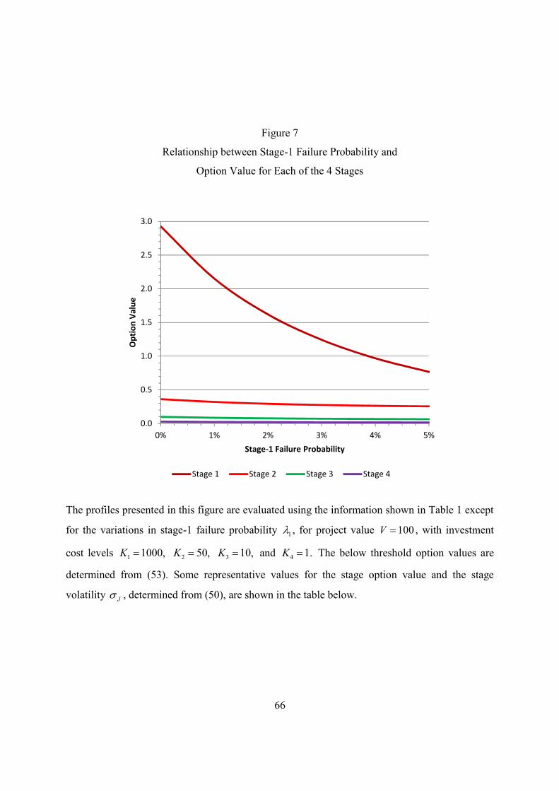
66

Figure 7

Relationship between Stage-1 Failure Probability and



for the variations in stage-1 failure probability 1 , for project value 100V , with investment

cost levels 1 1000,K 2 50,K 3 10,K and 4 1.K The below threshold option values are

determined from (53). Some representative values for the stage option value and the stage

volatility J , determined from (50), are shown in the table below.

0.0

0.5

1.0

1.5

2.0

2.5

3.0

0% 1% 2% 3% 4% 5%

Opt

ion

Val

ue

Stage-1 Failure Probability


67

Probability 1 0% 1% 2% 3% 4% 5%Volatility JStage 1 25.50% 25.50% 25.50% 25.50% 25.50% 25.50%Stage 2 49.18% 51.77% 54.20% 56.50% 58.69% 60.78%Stage 3 70.15% 70.14% 70.14% 70.13% 70.13% 70.12%Stage 4 85.35% 85.34% 85.34% 85.33% 85.33% 85.32%Option Value JFStage 1 2.92513 2.15077 1.61916 1.24255 0.96887 0.76576Stage 2 0.36082 0.31961 0.29251 0.27432 0.26223 0.25462Stage 3 0.09888 0.08530 0.07657 0.07081 0.06702 0.06465Stage 4 0.02682 0.02221 0.01935 0.01751 0.01632 0.01559

68

Figure 8

Relationship between Stage-1 Failure Probability and



for the variations in stage-1 failure probability 1 , with stage investment cost threshold levels

1ˆ 1000,K 2

ˆ 50,K 3ˆ 10,K and 4

ˆ 1K . The project value threshold levels JV from (43) or

(47). Some representative values of the project value threshold are shown in the table below.

Probability 1 0% 1% 2% 3% 4% 5%Project Value Threshold JVStage 1 2055.064 1951.987 1872.087 1808.020 1755.295 1711.002Stage 2 796.272 889.366 983.447 1081.686 1188.193 1309.051Stage 3 612.020 639.772 660.980 676.913 688.469 696.276Stage 4 310.861 324.867 335.547 343.548 349.329 353.210

0

500

1000

1500

2000

0% 1% 2% 3% 4% 5%

Proj

ect V

alue

Thr

esho

ld

Stage-1 Failure Probability


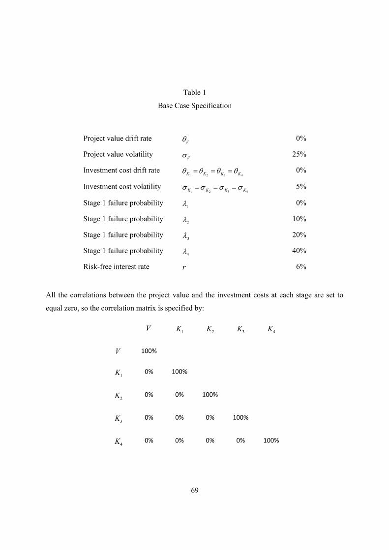
69

Table 1

Base Case Specification

Project value drift rate V 0%

Project value volatility V 25%

Investment cost drift rate1 2 3 4K K K K 0%

Investment cost volatility1 2 3 4K K K K 5%

Stage 1 failure probability 1 0%




Risk-free interest rate r 6%

All the correlations between the project value and the investment costs at each stage are set to

equal zero, so the correlation matrix is specified by:

V 1K 2K 3K 4K

V 100%

1K 0% 100%

2K 0% 0% 100%

3K 0% 0% 0% 100%

4K 0% 0% 0% 0% 100%

70

Table 2

Base Case Results

Panel A

Stage Volatility J J JB JA1J 25.50% 1.9478 0.25939 0.259392J 49.18% 1.4294 0.41741 0.060653J 70.15% 1.2176 0.56463 0.018614J 85.35% 1.2760 0.51362 0.00318

Panel B

Stage J 1J 2J 3J 4J1J 1.9478 -0.94782J 2.7843 -1.3548 -0.42943J 3.3901 -1.6496 -0.5229 -0.21764J 4.3257 -2.1049 -0.6672 -0.2776 -0.2760

Panel C

Stage 1J 2J 3J 4J1J 1.00002J 0.4866 0.51343J 0.4866 0.1542 0.35924J 0.4866 0.1542 0.0642 0.2950

Panel D

Stage 1 1 1J J J ˆJK JV

1J 1000 2055.0642J 3.1549 50 796.2723J 2.4029 10 612.0204J 1.0061 1 310.861

The values presented in this table are evaluated using the information shown in Table 1, with

stage investment cost threshold levels 1ˆ 1000,K 2

ˆ 50,K 3ˆ 10,K and 4

ˆ 1K . The threshold

71

levels chosen are selected arbitrarily while obeying the lower bound condition JLB (48). The

quantities in Panel A are determined from (50) for J , (49) for J , (51) for JB , and (52) for JA

; the J and the IJ in Panel B from (40); the IJ in Panel C from (44); and in Panel D, the JLB

from (48) and the project value threshold levels JV from (43) or (47).

72

Table 3

Stage Option Values JF V for Various Project Values

at each of the 4 Stages

V 1 1,F V K 2 1 2,F F K 3 2 3,F F K 4 3 4,F F K0 0.000 0.000 0.000 0.000100 2.925 0.361 0.099 0.027200 11.285 2.486 1.037 0.538300 24.859 7.686 4.098 3.107400 43.535 17.123 10.869 9.869500 67.237 31.872 23.158 22.158600 95.904 52.950 42.968 41.968700 129.490 81.332 71.332 70.332800 167.955 117.955 107.955 106.955900 211.265 161.265 151.265 150.2651000 259.391 209.391 199.391 198.3911200 369.985 319.985 309.985 308.9851400 499.556 449.556 439.556 438.5561600 647.950 597.950 587.950 586.9501800 815.036 765.036 755.036 754.0362000 1000.700 950.700 940.700 939.7002200 1200.000 1150.000 1140.000 1139.0002400 1400.000 1350.000 1340.000 1339.000

The values presented in this table are evaluated using the information shown in Table 1 and for

the specified project values V , with the investment cost levels 1 1000,K 2 50,K 3 10,K

and 4 1.K The option values are determined from (53). The bordered cells represent above

threshold option values while the cells without a border represent below threshold option values.

Table 4

Impact of Variations in the Investment Cost Volatility at Stage-2

on the Option Value, Project Value Threshold and Volatility

at each of the 4 Stages

73

Volatility2K 0.0% 5.0% 10.0% 15.0% 20.0%

Option Value JFStage 1 2.9251 2.9251 2.9251 2.9251 2.9251Stage 2 0.3569 0.3608 0.3726 0.3920 0.4188Stage 3 0.0978 0.0989 0.1023 0.1079 0.1157Stage 4 0.0265 0.0268 0.0279 0.0297 0.0322Threshold JVStage 1 2055.064 2055.064 2055.064 2055.064 2055.064Stage 2 794.474 796.272 801.626 810.426 822.501Stage 3 612.622 612.020 610.232 607.317 603.370Stage 4 311.443 310.861 309.147 306.398 302.759Volatility JStage 1 25.50% 25.50% 25.50% 25.50% 25.50%Stage 2 48.93% 49.18% 49.94% 51.17% 52.86%Stage 3 70.25% 70.15% 69.85% 69.39% 68.78%Stage 4 85.44% 85.35% 85.06% 84.62% 84.02%

The values presented in this table are evaluated using the information shown in Table 1. The

stage volatility J is determined from (50); the project value threshold JV from (43) or (47),

with investment cost threshold levels 1ˆ 1000,K 2

ˆ 50,K 3ˆ 10,K and 4

ˆ 1K , and the below

threshold option value at 100V from (53), with investment cost levels 1 1000,K 2 50,K

3 10,K and 4 1.K

74

Table 5

The Effect of Variations in the Investment Cost Correlation on

the Stage Volatility, Option Value and Project Value Threshold

for Each of the Four Stages

Correlation -100% -50% 0% 50% 100%Volatility JStage 1 25.50% 25.50% 25.50% 25.50% 25.50%Stage 2 48.70% 48.94% 49.18% 49.42% 49.66%Stage 3 69.55% 69.85% 70.15% 70.44% 70.73%Stage 4 84.70% 85.03% 85.35% 85.66% 85.98%Option Value JFStage 1 2.92513 2.92513 2.92513 2.92513 2.92513Stage 2 0.35336 0.35709 0.36082 0.36454 0.36825Stage 3 0.09534 0.09711 0.09888 0.10067 0.10245Stage 4 0.02537 0.02609 0.02682 0.02756 0.02831Project Value Threshold JVStage 1 2055.064 2055.064 2055.064 2055.064 2055.064Stage 2 792.859 794.568 796.272 797.970 799.662Stage 3 610.803 611.414 612.020 612.621 613.219Stage 4 311.682 311.269 310.861 310.456 310.056

The values presented in this table are evaluated using the information shown in Table 1, except

for the variations in correlation where1 2 1 3 1 4 2 3 2 4 3 4K K K K K K K K K K K K . The

stage volatility J is determined from (50); the project value threshold JV from (43) or (47),

with investment cost threshold levels 1ˆ 1000,K 2

ˆ 50,K 3ˆ 10,K and 4

ˆ 1K , and the below


3 10,K and 4 1.K

75

Table 6

The Effect of Variations in the Investment Cost Correlation on



Correlation 0 12 13 14 123 1234Volatility JStage 1 25.50% 25.50% 25.50% 25.50% 25.50% 25.50%Stage 2 49.18% 49.66% 49.18% 49.18% 49.66% 49.66%Stage 3 70.15% 70.10% 70.63% 70.15% 70.73% 70.73%Stage 4 85.35% 85.31% 85.33% 85.83% 85.28% 85.98%Option Value JFStage 1 2.92513 2.92513 2.92513 2.92513 2.92513 2.92513Stage 2 0.36082 0.36825 0.36082 0.36082 0.36825 0.36825Stage 3 0.09888 0.10129 0.09975 0.09888 0.10245 0.10245Stage 4 0.02682 0.02764 0.02711 0.02700 0.02804 0.02831Project Value Threshold JVStage 1 2055.064 2055.064 2055.064 2055.064 2055.064 2055.064Stage 2 796.272 799.662 796.272 796.272 799.662 799.662Stage 3 612.020 611.319 613.467 612.020 613.219 613.219Stage 4 310.861 309.813 310.544 311.318 309.399 310.056

The values for column “0” presented in this table are evaluated using the information shown in

Table 1, for column “12” with1 2

1K K , for column “13” with1 3

1K K , for column “14” with

1 41K K , for column “123” with

1 2 1 3 2 31K K K K K K , for column “1234” with

1 2 1 3 1 4 2 3 2 4 3 41K K K K K K K K K K K K . The stage volatility J is determined from (50);

the project value threshold JV from (43) or (47), with investment cost threshold levels

1ˆ 1000,K 2

ˆ 50,K 3ˆ 10,K and 4

ˆ 1K ; and the below threshold option value at 100V from

(53), with investment cost levels 1 1000,K 2 50,K 3 10,K and 4 1.K

77

Table 7

The Effect of Adverse Variations in the Stage-2 Failure Probability on



Probability 2 10% 11% 12% 13% 14% 15%Volatility JStage 1 25.50% 25.50% 25.50% 25.50% 25.50% 25.50%Stage 2 49.18% 49.18% 49.18% 49.18% 49.18% 49.18%Stage 3 70.15% 71.84% 73.49% 75.09% 76.65% 78.18%Stage 4 85.35% 85.35% 85.35% 85.35% 85.34% 85.34%Option Value JFStage 1 2.92513 2.92513 2.92513 2.92513 2.92513 2.92513Stage 2 0.36082 0.31403 0.27482 0.24171 0.21355 0.18943Stage 3 0.09888 0.09711 0.09601 0.09548 0.09546 0.09594Stage 4 0.02682 0.02621 0.02583 0.02565 0.02564 0.02581Project Value Threshold JVStage 1 2055.064 2055.064 2055.064 2055.064 2055.064 2055.064Stage 2 796.272 774.667 756.092 739.921 725.695 713.064Stage 3 612.020 641.677 673.591 708.832 748.964 796.463Stage 4 310.861 312.536 313.608 314.137 314.165 313.715

The values presented in this table are evaluated using the information shown in Table 1, except

for the adverse variations in the stage-2 failure probability 2 as specified in the table. The stage

volatility J is determined from (50); the project value threshold JV from (43) or (47), with

investment cost threshold levels 1ˆ 1000,K 2

ˆ 50,K 3ˆ 10,K and 4

ˆ 1K ; and the below


3 10,K and 4 1.K

78

References

Adkins, R., and D. Paxson. "Renewing assets with uncertain revenues and operating costs."Journal of Financial and Quantitative Analysis 46 (2011), 785-813.Agliardi, E., and R. Agliadi. "A generalization of the Geske formula for compound options."Mathematical Social Sciences 45 (2003), 75-82.Andergassen, R., and L. Sereno. "Valuation of N-stage investments under jump-diffusionprocesses." Computational Economics 39 (2012), 289-313.Bar-Ilan, A., and W. C. Strange. "A model of sequential investment." Journal of EconomicDynamics and Control 22 (1998), 437-463.Carr, P. "The valuation of sequential exchange opportunities." Journal of Finance 43 (1988),1235-1256.Cassimon, D., M. De Backer, P. J. Engelen, M. Van Wouwe, and V. Yordanov. "Incorporatingtechnical risk in compound real option models to value a pharmaceutical R&D licensingopportunity." Research Policy 40 (2011), 1200-1216.Cassimon, D., P. J. Engelen, L. Thomassen, and M. Van Wouwe. "The valuation of a N.D.A.using a 6-fold compound option." Research Policy 33 (2004), 41-51.Childs, P. D., and A. J. Triantis. "Dynamic R&D investment policies." Management Science 45(1999), 1359-1377.Cortazar, G., E. S. Schwartz, and J. Casassus. "Optimal exploration investments under price andgeological-technical uncertainty: a real options model." In Real R&D Options, D. Paxson, ed.Oxford: Butterworth-Heinemann (2003).Cortelezzi, F., and G. Villani. "Valuation of R&D Sequential Exchange Options Using MonteCarlo Approach." Computational Economics 33 (2009), 209-236.Dixit, A. K., and R. S. Pindyck. Investment under Uncertainty. Princeton, NJ: PrincetonUniversity Press (1994).Geske, R. "The valuation of compound options." Journal of Financial Economics 7 (1979), 63-81.Ghosh, S., and M. D. Troutt. "Complex compound option models – Can practitioners trulyoperationalize them?" European Journal of Operational Research 222 (2012), 542-552.Kort, P. M., P. Murto, and G. Pawlina. "Uncertainty and stepwise investment." EuropeanJournal of Operational Research 202 (2010), 196-203.Lee, J., and D. A. Paxson. "Valuation of R&D real American sequential exchange options."R&D Management 31 (2001), 191-201.Lee, M.-Y., F.-B. Yeh, and A.-P. Chen. "The generalized sequential compound options pricingand sensitivity analysis." Mathematical Social Sciences 55 (2008), 38-54.Majd, S., and R. S. Pindyck. "Time to build, option value, and investment decisions." Journal ofFinancial Economics 18 (1987), 7-27.Margrabe, W. "The value of an option to exchange one asset for another." Journal of Finance 33(1978), 177-186.McDonald, R. L., and D. R. Siegel. "Investment and the valuation of firms when there is anoption to shut down." International Economic Review 26 (1985), 331-349.—. "The value of waiting to invest." Quarterly Journal of Economics 101 (1986), 707-728.Merton, R. C. "Theory of rational option pricing." Bell Journal of Economics and ManagementScience 4 (1973), 141-183.

79

Pennings, E., and L. Sereno. "Evaluating pharmaceutical R&D under technical and economicuncertainty." European Journal of Operational Research 212 (2011), 374-385.Pindyck, R. S. "Investments of uncertain cost." Journal of Financial Economics 34 (1993), 53-76.Samuelson, P. A. "Rational theory of warrant pricing." Industrial Management Review 6 (1965),13-32.Schwartz, E. S., and M. Moon. "Evaluating research and development investments." In ProjectFlexibility, Agency, and Competition, M. J. Brennan and L. Trigeorgis, eds. Oxford: OxfordUniversity Press (2000).Sydsæter, K., and P. Hammond. Essential mathematics for economic analysis. Harlow, England:Prentice-Hall (2006).Sydsæter, K., P. Hammond, A. Seierstad, and A. Strøm. Further Mathematics for EconomicAnalysis. London: FT Prentice Hall (2005).Tourinho, O. A. F. "The option value of reserves of natural resources." In Research Program inFinance Working Papers: Graduate School of Business Administration, University of Californiaat Berkeley (1979).

an analytical model for a sequential investment opportunity · manchester business school ... an...

Documents