an appa-based descent method with optimal step-sizes for monotone variational inequalities

Available online at www.sciencedirect.com

European Journal of Operational Research 186 (2008) 486–495

www.elsevier.com/locate/ejor

Continuous Optimization

An APPA-based descent method with optimal step-sizesfor monotone variational inequalities

Min Li a, Xiao-Ming Yuan b,*

a Department of Mathematics, Nanjing University, Nanjing 210093, Chinab Department of Management Science, Antai College of Economics and Management, Shanghai Jiao Tong University,

Shanghai 200052, China

Received 2 April 2006; accepted 6 February 2007Available online 30 March 2007

Abstract

To solve monotone variational inequalities, some existing APPA-based descent methods utilize the iterates generated bythe well-known approximate proximal point algorithms (APPA) to construct descent directions. This paper aims atimproving these APPA-based descent methods by incorporating optimal step-sizes in both the extra-gradient steps andthe descent steps. Global convergence is proved under mild assumptions. The superiority to existing methods is verifiedboth theoretically and computationally.� 2007 Elsevier B.V. All rights reserved.

Keywords: Variational inequalities; Proximal point algorithm; Descent method; Optimal step-size

1. Introduction

The finite-dimensional variational inequality problem VI(C,F) is to determine a vector x 2 C such that

0377-2

doi:10

* CoE-m

VIðC; F Þ ðx0 � xÞTF ðxÞP 0; 8x0 2 C; ð1Þ

where C is assumed to be a nonempty closed convex subset of Rn. Throughout we assume that F is a contin-uous and monotone mapping from Rn into itself, and the solution set of VI(C,F) (denoted by C*) is not empty.Serving as the uniform mathematical model of various applications arising in engineering, economic, transpor-tation, etc., VI(C,F) has been receiving much attention of researchers not only from optimization community,but also from application fields.

Among effective numerical approaches to solving VI(C,F) is the Proximal Point Algorithm (PPA), whichwas presented originally by Martinet [8] (see, e.g. [1,2,9,10,13]) for finding roots of a maximal monotone

217/$ - see front matter � 2007 Elsevier B.V. All rights reserved.

.1016/j.ejor.2007.02.042

rresponding author. Tel.: +86 21 52301397.ail addresses: [email protected] (M. Li), [email protected] (X.-M. Yuan).

mailto:[email protected]

mailto:[email protected]

M. Li, X.-M. Yuan / European Journal of Operational Research 186 (2008) 486–495 487

operator in Rn. In particular, let xk 2 C be the current approximation of a solution of VI(C,F), PPA generatesthe new iterate xkþ1 by solving the following auxiliary VI:

ðPPAÞ ðx0 � xÞTF kðxÞP 0; 8x0 2 C; ð2Þ

where

F kðxÞ ¼ ðx� xkÞ þ kkF ðxÞ ð3Þ

and kk 2 ½kmin;þ1Þ with kmin being a positive constant. Let P Cð�Þ denote the projection onto C in the Euclid-ean norm, then (see, e.g. [3]) solving (2) is equivalent to solving the following equation:

x ¼ P C½xk � kkF ðxÞ�; ð4Þ

which is a nonsmooth equation and implicit scheme. Therefore, without a special structure, the new iteratexkþ1 cannot be computed directly via (4). Since this difficulty makes straightforward applications of PPAimpractical in many cases, it is of importance to develop PPA with improved practical characteristics. Oneeffort in this sense is to find approximate solutions of (2) instead of solving it exactly, hence results in manyapproximate PPAs (APPA), see, e.g., [4,6,7,10,11]. For given xk 2 C, kk > 0 and under some inexactnessrestrictions, the APPA-type method in [11] (denoted by the SS-method) finds an approximate solution of(2) (denoted by yk) in the sense that

yk � P C½yk � F kðykÞ�: ð5Þ

Then the new iterate xkþ1SS is generated by correcting yk with the so-called extra-gradient step:

xkþ1SS :¼ P C½yk � F kðykÞ� ¼ð3Þ P C½xk � kkF ðykÞ�: ð6Þ

With a relaxed inexactness restriction for solving (5), authors in [7] prove that

xk � P C½xk � kkF ðykÞ� ð7Þ

is a descent direction of kx� x�k2 at xk (x� 2 C�), and so they develop the SS-method by contributing an inter-esting APPA-based descent method (denoted by the HYY-method) for solving VI(C,F). More specifically, theHYY-method generates the new iterate xkþ1

HYY via the following scheme:

xkþ1HYY ¼ P C½xk � sðxk � P C½xk � kkF ðykÞ�Þ�: ð8Þ

Note that the HYY-method reduces to the SS-method when s = 1 (which is proved to be possible in [7]). Thenumerical results reported in [7] show that efforts of identifying the optimal step-size s�HYY along the descentdirection (7) lead to attractive numerical improvements. This fact triggers us to investigate the selection ofoptimal step-sizes in both the extra-gradient step (6) and the descent step (8) to accelerate convergence. In par-ticular, a new APPA-based descent method with optimal step-sizes in both (6) and (8) will be presented. The-oretical comparison to the HYY-method shows the superiority of the new method. The preferences to the SS-method and the HYY-method are verified by numerical experiments for network equilibrium problems arisingin transportation.

The rest of this paper is organized as follows: in Section 2, we summarize some preliminaries of variationalinequalities. In Section 3, the new APPA-based descent method is presented. We investigate the selection ofoptimal step-sizes of the new method in Section 4. Then convergence of the new method is proved in Section5. In Section 6, the new method is compared to the HYY-method, whose theoretical assertions are verified bythe numerical results reported in Section 7. Finally some conclusions are drawn in Section 8.

2. Preliminaries

Recall that P Cð�Þ denotes the projection onto C in the Euclidean norm, i.e.,

P CðzÞ ¼ argminfkz� xkjx 2 Cg; 8z 2 Rn:

Some fundamental inequalities are listed below without proof (see, e.g., [3]).

488 M. Li, X.-M. Yuan / European Journal of Operational Research 186 (2008) 486–495

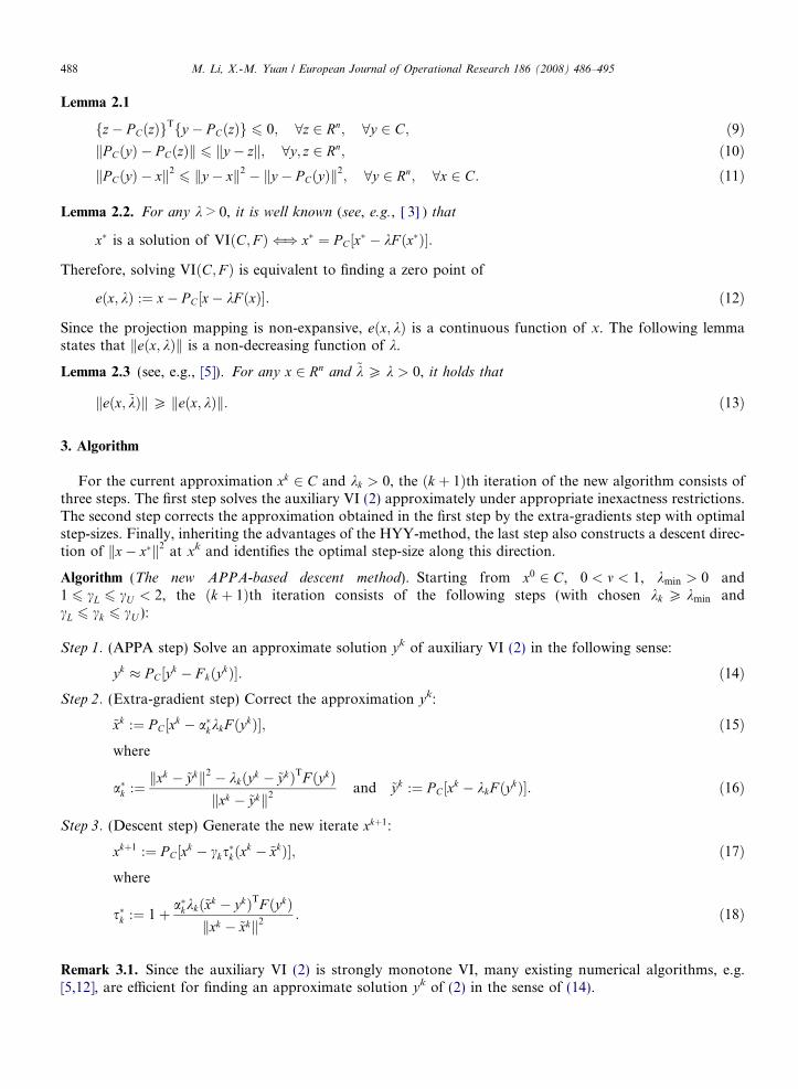
Lemma 2.1

fz� P CðzÞgTfy � P CðzÞg 6 0; 8z 2 Rn; 8y 2 C; ð9ÞkP CðyÞ � P CðzÞk 6 ky � zk; 8y; z 2 Rn; ð10ÞkP CðyÞ � xk2

6 ky � xk2 � ky � P CðyÞk2; 8y 2 Rn; 8x 2 C: ð11Þ

Lemma 2.2. For any k > 0, it is well known (see, e.g., [3]) that

x� is a solution of VIðC; F Þ () x� ¼ P C½x� � kF ðx�Þ�:

Therefore, solving VIðC; F Þ is equivalent to finding a zero point of

eðx; kÞ :¼ x� P C½x� kF ðxÞ�: ð12Þ

Since the projection mapping is non-expansive, eðx; kÞ is a continuous function of x. The following lemmastates that keðx; kÞk is a non-decreasing function of k.

Lemma 2.3 (see, e.g., [5]). For any x 2 Rn and ~k P k > 0, it holds that

keðx; ~kÞkP keðx; kÞk: ð13Þ

3. Algorithm

For the current approximation xk 2 C and kk > 0, the ðk þ 1Þth iteration of the new algorithm consists ofthree steps. The first step solves the auxiliary VI (2) approximately under appropriate inexactness restrictions.The second step corrects the approximation obtained in the first step by the extra-gradients step with optimalstep-sizes. Finally, inheriting the advantages of the HYY-method, the last step also constructs a descent direc-tion of kx� x�k2 at xk and identifies the optimal step-size along this direction.

Algorithm (The new APPA-based descent method). Starting from x0 2 C, 0 < m < 1, kmin > 0 and1 6 cL 6 cU < 2, the ðk þ 1Þth iteration consists of the following steps (with chosen kk P kmin andcL 6 ck 6 cU ):

Step 1: (APPA step) Solve an approximate solution yk of auxiliary VI (2) in the following sense:

yk � P C½yk � F kðykÞ�: ð14Þ
Step 2: (Extra-gradient step) Correct the approximation yk:
~xk :¼ P C½xk � a�kkkF ðykÞ�; ð15Þwhere

a�k :¼ kxk � ~ykk2 � kkðyk � ~ykÞTF ðykÞ

kxk � ~ykk2and ~yk :¼ P C½xk � kkF ðykÞ�: ð16Þ

Step 3: (Descent step) Generate the new iterate xkþ1:

xkþ1 :¼ P C½xk � cks�kðxk � ~xkÞ�; ð17Þ

where

s�k :¼ 1þ a�kkkð~xk � ykÞTF ðykÞkxk � ~xkk2

: ð18Þ

Remark 3.1. Since the auxiliary VI (2) is strongly monotone VI, many existing numerical algorithms, e.g.[5,12], are efficient for finding an approximate solution yk of (2) in the sense of (14).


Remark 3.2. For the justification of comparing the new method to the HYY-method and revealing theimprovements in terms of optimal step-sizes, in the APPA step we use the same inexactness restriction asthe HYY-method in [7], i.e., yk is solved under the following restriction:

DðykÞ 6 m�kxk � ykk2 þ kxk � ~ykk2

�; ð19Þ

where

DðykÞ ¼ 2ðyk � ~ykÞTF kðykÞ � kyk � ~ykk2: ð20Þ

4. The optimal step-sizes

This section concentrates on investigating optimal step-sizes in order to accelerate convergence of the newmethod. To justify the reason of choosing the optimal step-size a�k in the extra-gradient step (15), we start fromthe following general form of the extra-gradient step:

~xkðaÞ :¼ P C½xk � akkF ðykÞ�; 8a > 0: ð21Þ
Let
HkðaÞ :¼ kxk � x�k2 � k~xkðaÞ � x�k2;

which measures the progress made by the extra-gradient step.Note that HkðaÞ is a function of the step-size a. It is natural to consider maximizing this function by choos-

ing an optimal parameter a. The solution x* is not known, so we cannot maximize HkðaÞ directly. The follow-ing lemma gives an estimate of HkðaÞ which does not include the unknown solution x*.

Lemma 4.1. Let x* be an arbitrary point in C*. If the step-size in the extra-gradient step is taken a > 0, then we

have

HkðaÞ ¼ kxk � x�k2 � k~xkðaÞ � x�k2 P � kðaÞP WkðaÞ; ð22Þ
where
� kðaÞ :¼ kxk � ~xkðaÞk2 þ 2akkf~xkðaÞ � ykgT F ðykÞ; ð23Þ

WkðaÞ :¼ 2afkxk � ~ykk2 � kkðyk � ~ykÞT F ðykÞg � a2kxk � ~ykk2: ð24Þ

Proof. Since x� 2 C and ~xkðaÞ ¼ P C½xk � akkF ðykÞ�, it follows from (11) that

k~xkðaÞ � x�k26 kxk � akkF ðykÞ � x�k2 � kxk � akkF ðykÞ � ~xkðaÞk2

: ð25Þ

Consequently, using the definition of HkðaÞ, we get

HkðaÞP kxk � x�k2 þ kxk � ~xkðaÞ � akkF ðykÞk2 � kxk � x� � akkF ðykÞk2

¼ kxk � ~xkðaÞk2 þ 2akkf~xkðaÞ � x�gTF ðykÞ: ð26Þ

Since x� 2 C�, using the monotonicity of F, we have

ðyk � x�ÞTF ðykÞP ðyk � x�ÞTF ðx�ÞP 0;

and consequently

ð~xkðaÞ � x�ÞTF ðykÞP ð~xkðaÞ � ykÞTF ðykÞ: ð27Þ

Applying (27) to the last term in the right side of (26), we obtain

HkðaÞP kxk � ~xkðaÞk2 þ 2akkf~xkðaÞ � ykgTF ðykÞ: ð28Þ


The first assertion follows immediately. Since ~yk ¼ P C½xk � kkF ðykÞ� (see (16)) and ~xkðaÞ 2 C, it follows from (9)that for any a > 0,

0 P 2af~xkðaÞ � ~ykgTf½xk � kkF ðykÞ� � ~ykg: ð29Þ

Adding (23) and (29), we obtain

� kðaÞP kxk � ~xkðaÞk2 þ 2af~xkðaÞ � ~ykgTðxk � ~ykÞ � 2akkðyk � ~ykÞTF ðykÞ: ð30Þ

Regrouping the first two terms of the right-hand-side of (30), we get

kxk � ~xkðaÞk2 þ 2af~xkðaÞ � ~ykgTðxk � ~ykÞ ¼ kxk � ~xkðaÞk2 þ 2afð~xkðaÞ � xkÞ þ ðxk � ~ykÞgTðxk � ~ykÞ

¼ kxk � ~xkðaÞk2 þ 2af~xkðaÞ � xkgTðxk � ~ykÞ þ 2akxk � ~ykk2

¼ kðxk � ~xkðaÞÞ � aðxk � ~ykÞk2 þ ð2a� a2Þkxk � ~ykk2: ð31Þ

Substituting (31) into (30), we obtain

� kðaÞP 2afkxk � ~ykk2 � kkðyk � ~ykÞTF ðykÞg � a2kxk � ~ykk2

and the second assertion is proved. h

This lemma provides the basis of the selection of the optimal step-size in the extra-gradient step (15). Notethat WkðaÞ is the profit-function since it is a lower-bound of the progress obtained by the extra-gradient step(15). This lemma motivates us to maximize the profit-function WkðaÞ to accelerate convergence of the newmethod. Since WkðaÞ is a quadratic function of a, it reaches its maximum at

a�k ¼kxk � ~ykk2 � kkðyk � ~ykÞTF ðykÞ

kxk � ~ykk2;

with

Wkða�kÞ ¼ a�kfkxk � ~ykk2 � kkðyk � ~ykÞTF ðykÞg; ð32Þ

we prefer to a�k in the extra-gradient step.The following two lemmas verify that �ðxk � ~xkÞ is a descent direction of kx� x�k2 at xk.

Lemma 4.2

Wkða�kÞPð1� mÞ2

4ðkxk � ykk2 þ kxk � ~ykk2Þ; 8k P 0: ð33Þ

Proof. See the proof of Proposition 3.1 and (3.17) in [7]. h

Lemma 4.3. Let x* be an arbitrary point in C* and ~xk ¼ ~xkða�kÞ be generated by (15). Then we have

2ðxk � x�ÞT ðxk � ~xkÞP � kða�kÞ þ kxk � ~xkk2: ð34Þ

Proof. Note that

~xk � x� ¼ ðxk � x�Þ � ðxk � ~xkÞ:

Substituting this into (22), we have

2ðxk � x�ÞTðxk � ~xkÞ � kxk � ~xkk2 P � kða�kÞ

and thus complete the proof. h


Remark 4.3. It is trivial to observe that the new method will terminate with a desirable solution whenxk ¼ ~xk ¼ yk ¼ ~yk. Hence, according to (22), (33) and (34), we conclude that

ðxk � x�ÞTðxk � ~xkÞP 0;

which implies that �ðxk � ~xkÞ is a descent direction of kx� x�k2 at xk.

Similarly, we start from the general form of the descent step

xkþ1ðsÞ :¼ P C½xk � sðxk � ~xkÞ�
to analyze the optimal step-size in the descent step (17). The following theorem estimates the ‘‘progress’’ in thesense of Euclidean distance made by the new iterate and thus motivates us to investigate the selection of theoptimal step-size s�k in the descent step (17).
Theorem 4.1. Let x* be an arbitrary point in C* and the step-size in the extra-gradient step be taken a�k > 0, i.e.,

(15), then if the step-size in the descent step is taken s > 0, we have

KkðsÞ :¼ kxk � x�k2 � kxkþ1ðsÞ � x�k2 P UkðsÞ; ð35Þ

where

UkðsÞ :¼ sf� kða�kÞ þ kxk � ~xkk2g � s2kxk � ~xkk2 ð36Þ

and � kðaÞ is defined in (23).

Proof. Since xkþ1ðsÞ :¼ P C½xk � sðxk � ~xkÞ� and x� 2 C, it follows from (10) that

kxk � x� � sðxk � ~xkÞkP kxkþ1ðsÞ � x�k:
Consequently, we have
KkðsÞP kxk � x�k2 � kxk � x� � sðxk � ~xkÞk2 ¼ 2sðxk � x�ÞTðxk � ~xkÞ � s2kxk � ~xkk2: ð37Þ

Inequality (35) follows from Lemma 4.3 and (36) directly and the proof is complete. h

Since UkðsÞ is a quadratic function of s, it reaches its maximum at

s�k ¼� kða�kÞ þ kxk � ~xkk2

2kxk � ~xkk2¼ð23Þ

1þ a�kkkð~xk � ykÞTF ðykÞkxk � ~xkk2

: ð38Þ

To maximize the profit-function UkðsÞ, it is justified to use s�k defined in (38) as the optimal step-size in thedescent step (17). From numerical point of view, it is necessary to attach a relax factor to the optimal step-size s�k obtained theoretically to achieve faster convergence. The following theorem concerns how to choosethe relax factor.

Theorem 4.2. Let x* be an arbitrary point in C*, c be a positive constant and s�k be defined in (38). Let ~xk be

generated by (15) and xkþ1ðcs�kÞ ¼ P C½xk � cs�kðxk � ~xkÞ�, then we have

kxkþ1ðcs�kÞ � x�k26 kxk � x�k2 � cð2� cÞ

4fc0ðkxk � ykk2 þ kxk � ~ykk2Þ þ kxk � ~xkk2g;

where

c0 ¼ð1� mÞ2

4: ð39Þ

Proof. First, from (36) and (38), we have

Ukðs�kÞ ¼1

2s�kf� kða�kÞ þ kxk � ~xkk2g: ð40Þ


It follows from Lemmas 4.1, 4.2 and (38) that

s�k P1

2and Ukðs�kÞP

1

4fc0ðkxk � ykk2 þ kxk � ~ykk2Þ þ kxk � ~xkk2g; ð41Þ

where c0 is defined in (39).Note that

Ukðcs�kÞ ¼ð36Þ

cs�kf� kða�kÞ þ kxk � ~xkk2g � ðc2s�kÞðs�kkxk � ~xkk2Þ

¼ð38Þðcs�k �1

2c2s�kÞf� kða�kÞ þ kxk � ~xkk2g ¼ð40Þ

cð2� cÞUkðs�kÞ: ð42Þ

The assertion follows from (35), (42) and (41) directly. h

Theorem 4.2 shows theoretically that any c 2 ð0; 2Þ guarantees that the new iterate makes progress to asolution. Therefore, in practical computation, we choose sk ¼ cks

�k with ck 2 ½cL; cU � � ½1; 2Þ as the step-size

in (17). We need to point out that from numerical experiments, c 2 ½1; 2Þ is much preferable since it leadsto better numerical performance.

5. Convergence

In this section we mainly focus on investigating the convergence of the proposed method. The followinglemma concerns the contractive property of the sequence generated by the new method.

Lemma 5.1. Let x* be an arbitrary point in C* and the sequence fxkg be generated by the new method. Then thereexists a positive constant c such that

kxkþ1 � x�k26 kxk � x�k2 � c � fkxk � ykk2 þ kxk � ~ykk2 þ kxk � ~xkk2g: ð43Þ

Proof. It follows from Theorem 4.2 and ck 2 ½cL; cU � that

kxkþ1 � x�k26 kxk � x�k2 � cLð2� cU Þ

4fc0ðkxk � ykk2 þ kxk � ~ykk2Þ þ kxk � ~xkk2g: ð44Þ

Recall that m 2 ð0; 1Þ. Then we have c0 2 ð0; 1=4Þ from (39). Therefore, the assertion (43) is satisfied with

c ¼ cLð2� cU Þ4

c0: �

Now we are at the stage to prove the the convergence of the new method.

Theorem 5.1. The sequence fxkg generated by the new method converges to a solution of VI(C,F).

Proof. First, from (43) we get

limk!1kxk � ykk ¼ 0 and lim

k!1kxk � ~ykk ¼ 0: ð45Þ

Moreover we have

limk!1kyk � ~ykk ¼ lim

k!1kðxk � ~ykÞ � ðxk � ykÞk 6 lim

k!1kxk � ~ykk þ lim

k!1kxk � ykk ¼ 0: ð46Þ

Note that

keðyk; kminÞk 6ð13Þkeðyk; kkÞk ¼ kyk � P C½yk � kkF ðykÞ�k ¼ kyk � ~yk þ ~yk � P C½yk � kkF ðykÞ�k

6

ð16Þkyk � ~ykk þ kP C½xk � kkF ðykÞ� � P C½yk � kkF ðykÞ�k 6

ð10Þkyk � ~ykk þ kxk � ykk: ð47Þ


It follows from (45)–(47) that

limk!1

eðyk; kminÞ ¼ 0:

Again, it follows from (43) that the sequence fxkg is bounded. Let x1 be a cluster point of fxkg and the sub-sequence fxkjg converges to x1. From (45), we know that the subsequence fykjg also converges to x1. Notethat eð�; kminÞ is continuous, so we have

eðx1; kminÞ ¼ limj!1

eðykj ; kminÞ ¼ 0;

which means that x1 is a solution point of VI(C,F). Because the subsequence fxkjg converges to x1, for anarbitrary scalar e > 0, there exists a kl > 0 such that

kxkl � x1k 6 e:

On the other hand, since x1 2 C� , it follows from (43) that

kxk � x1k 6 kxkl � x1k 6 e 8k P kl;

and thus the sequence fxkg converges to x1, which is a solution point of VI(C,F). h

6. Comparison

Recall that at the ðk þ 1Þth iteration, the HYY-method with the relax factor ck generates the new iteratexkþ1

HYY via the following scheme:

xkþ1HYY ¼ P C½xk � cks

�HYYðxk � P C½xk � kkF ðykÞ�Þ�; ð48Þ

where

s�HYY ¼kxk � ~ykk2 � kkðyk � ~ykÞTF ðykÞ

kxk � ~ykk2¼ð16Þ

a�k : ð49Þ

Although the HYY-method identifies the optimal step-size in the descent step, it does not do so in the extra-gradient step. This fact makes us expect that the new method has better numerical performance. In this sectionwe compare these two methods and focus on the theoretical analysis. Throughout this comparison, we assumethat these two methods take the same values of ck at each iteration.

The following lemma regarding the progress of each iterate generated by the HYY-method is proved in [7].

Lemma 6.1. Let x* be an arbitrary point in C*, xk 2 C and xkþ1HYY be given by the HYY-method (48) and (49).

Then we have

HkHYY :¼ kxk � x�k2 � kxkþ1

HYY � x�k2 P Wkðcks�HYYÞ; ð50Þ

where Wkð�Þ is defined in (24).

By simple manipulations we obtain

Wkðcks�HYYÞ ¼

ð24Þ2cks

�HYYfkxk � ~ykk2 � kkðyk � ~ykÞTF ðykÞg � ðc2

ks�HYYÞðs�HYYkxk � ~ykk2Þ

¼ð32Þð2cks�HYY � c2

ks�HYYÞfkxk � ~ykk2 � kkðyk � ~ykÞTF ðykÞg ¼ð32Þ

ckð2� ckÞWkðs�HYYÞ: ð51Þ

From now on we let xkþ1New denote the new iterate generated by the new method. Then according to Theorem 4.1

we have

KkNew :¼ kxk � x�k2 � kxkþ1

New � x�k2 P Ukðcks�kÞ:

Obviously, it is meaningful to compare the lower-bounds Wkðcks�HYYÞ and Ukðcks

�kÞ in order to compare the

progress HkHYY and Kk

New made by these two methods. The following theorem indicates theoretically thatwe may expect the new method to make more progress than the HYY-method.

Table 1Iteration numbers and CPU time of different methods

Method No. of outer iterations No. of total inner iterations CPU time (seconds)

SS-method 20 182 0.19HYY-method 12 111 0.13New-method 10 70 0.09


Theorem 6.1. Let Wkð�Þ and Ukð�Þ be defined in (24) and (36), s�HYY and s�k be defined in (49) and (38),

respectively. Then we have

Ukðcks�kÞP Wkðcks

�HYYÞ:

Proof. It follows from (51) and (42) that

Wkðcks�HYYÞ ¼ ckð2� ckÞWkðs�HYYÞ and Ukðcks

�kÞ ¼ ckð2� ckÞUkðs�kÞ: ð52Þ

Since s�k defined in (38) is to maximize the profit-function UkðsÞ, we have

Ukðs�kÞP Ukð1Þ: ð53Þ
Note that
Ukð1Þ ¼ð36Þ

� kða�kÞPð22Þ

Wkða�kÞ ¼ð49Þ

Wkðs�HYYÞ: ð54Þ
The assertion of this theorem follows directly from (52)–(54). h
7. Numerical experiments

The purpose of this section is to verify previous theoretical assertions via numerical experiments. To com-pare to the HYY-method, we test the identical network equilibrium problem , which was studied in [7,14]. Weomit the description and data of the problem, which can be found in Section 5 of [7]. In fact, this problemreduces to the nonlinear complementarity problem in the space of path-flow pattern x:

find x� P 0 such that ðx� x�ÞTF ðx�ÞP 0; 8x P 0; ð55Þ
where the expression of the mapping F can also be found in Section 5 of [7].
For comparison, this problem is solved by the SS-method, the HYY-method and the new method, respec-tively. Since the HYY-method solves the approximate solution yk of the auxiliary VI (2) by the improvedextra-gradient method in [5], we also use the same method to obtain yk. Note that the mapping F ðxÞ containslogarithmic function. Hence, we begin with the starting point x0 ¼ ð1; 1; . . . ; 1Þ and take kk � 50, m = 0.8,ck 2 ½1; 2Þ. The programs written in Matlab were run on an IBM X31 notebook computer. The stopping cri-terion is keðxk; 1Þk 6 10�6 (see (12)). Achieving the identical optimal path flow and optimal link flow, therespective numbers of iterations and CPU time of different methods are reported in Table 1. Note that theinner iteration refers to the procedure of applying some existing numerical algorithm (e.g., the improvedextra-gradient method in [5]) to obtain yk in the APPA step (14).

The computational preferences to the SS-method and the HYY-method are revealed clearly in Table 1. Thenumerical results demonstrate that the selection of optimal step-sizes in both the extra-gradient step andthe descent step reduces considerable computational load of the APPA-based descent methods, and thus verifythe theoretical assertions presented previously.

8. Conclusion

This paper concentrates on improving some existing APPA-based descent methods by choosing optimalstep-sizes. As a result, a new APPA-based descent method is presented. The superiority to some existing meth-ods is verified both theoretically and computationally. Our research interests in the future include designing


effective numerical algorithms based on some general APPA-type methods and the idea presented in thispaper.

Acknowledgements

The authors are grateful to the anonymous referees for their valuable comments to improve the presenta-tion of this paper. This work was partially funded by NSFC Grant 10571083 and MOEC Grant 20060284001.The second author was supported by an internal grant of Antai College of Economics and Management,Shanghai Jiao Tong University.

References

[1] A. Auslender, M. Haddou, An interior proximal point method for convex linearly constrained problems and its extension tovariational inequalities, Mathematical Programming 71 (1995) 77–100.

[2] A. Auslender, M. Teboulle, S. Ben-Tiba, A logarithmic-quadratic proximal method for variational inequalities, ComputationalOptimization and Applications 12 (1999) 31–40.

[3] B.C. Eaves, On the basic theorem of complementarity, Mathematical Programming 1 (1971) 68–75.[4] J. Eckstein, Approximate iterations in Bregman-function-based proximal algorithms, Mathematical Programming 83 (1998) 113–123.[5] B.S. He, L.-Z. Liao, Improvements of some projection methods for monotone nonlinear variational inequalities, Journal of

Optimization Theory and Applications 112 (2002) 111–128.[6] B.S. He, L.-Z. Liao, Z.H. Yang, A new approximate proximal point algorithm for maximal monotone operator, Science in China,

Series A 46 (2) (2003) 200–206.[7] B.S. He, Z.H. Yang, X.M. Yuan, An approximate proximal-extragradient type method for monotone variational inequalities, Journal

of Mathematical Analysis and Applications 300 (2) (2004) 362–374.[8] B. Martinet, Regularization d’inequations Variationnelles par Approximations Succesives, Revue Francaise d’Informatique et de

Recherche Operationnelle 4 (1970) 154–159.[9] R.T. Rockafellar, Augmented Lagrangians and applications of the proximal point algorithm in convex programming, Mathematics of

Operations Research 1 (1976) 97–116.[10] R.T. Rockafellar, Monotone operators and the proximal point algorithm, SIAM Journal on Optimization 14 (5) (1976) 877–898.[11] M.V. Solodov, B.F. Svaiter, Error bounds for proximal point subproblems and associated inexact proximal point algorithms,

Mathematical Programming, Series B 88 (2000) 371–389.[12] K. Taji, M. Fukushima, T. Ibaraki, A globally convergent Newton method for solving strongly monotone variational inequalities,

Mathematical Programming 58 (1993) 369–383.[13] M. Teboulle, Convergence of proximal-like algorithms, SIAM Journal on Optimization 7 (1997) 1069–1083.[14] H. Yang, M.G.H. Bell, Traffic restraint, road pricing and network equilibrium, Transportation Research, Part B 31 (4) (1997) 303–

314.

an appa-based descent method with optimal step-sizes for monotone variational inequalities

Documents