Air Force Institute of TechnologyAFIT Scholar

Theses and Dissertations Student Graduate Works

3-22-2012

An Application of Course Scheduling in theBrazilian Air ForceJulio C. O. Lopes

Follow this and additional works at: https://scholar.afit.edu/etd

Part of the Engineering Education Commons

This Thesis is brought to you for free and open access by the Student Graduate Works at AFIT Scholar. It has been accepted for inclusion in Theses andDissertations by an authorized administrator of AFIT Scholar. For more information, please contact richard.mansfield@afit.edu.

Recommended CitationLopes, Julio C. O., "An Application of Course Scheduling in the Brazilian Air Force" (2012). Theses and Dissertations. 1222.https://scholar.afit.edu/etd/1222

AN APPLICATION OF COURSE SCHEDULING IN THE BRAZILIAN AIR FORCE

GRADUATE THESIS

Julio C O Lopes, Captain, BAF

AFIT-LSCM-ENS-12-09

DEPARTMENT OF THE AIR FORCE AIR UNIVERSITY

AIR FORCE INSTITUTE OF TECHNOLOGY

Wright-Patterson Air Force Base, Ohio DISTRIBUTION STATEMENT A: APPROVED FOR PUBLIC RELEASE; DISTRIBUTION UNLIMITED

The views expressed in this thesis are those of the author and do not reflect the official

policy or position of the Brazilian Air Force, Ministry of Defense, or the Brazilian

Government.

AFIT-LSCM-ENS-12-09

AN APPLICATION OF TIMETABLE PROBLEM IN THE BRAZILIAN AIR FORCE

THESIS

Presented to the Faculty

Graduate School of Logistics and Acquisition Management

Air Force Institute of Technology

Air University

Air Education and Training Command

In Partial Fulfillment of the Requirements for the

Degree of Master of Science

Julio C O Lopes, Captain, BAF

Mar 2012

DISTRIBUTION STATEMENT A:

APPROVED FOR PUBLIC RELEASE; DISTRIBUTION UNLIMITED

AFIT-LSCM-ENS-12-09

AN APPLICATION OF TIMETABLE PROBLEM IN THE BRAZILIAN AIR FORCE

Julio C O Lopes, MSC

Captain, BAF

Approved:

____________________________________ _______________ Deckro F. Richard , DBA (Chairman) Date ____________________________________ _______________ Johnson, Alan W., Ph.D. (Member) Date

iv

AFIT-LSCM-ENS-12-0912M

Abstract

The Institute of Logistic of the Brazilian Air Force (ILA) is responsible for

executing the technical courses related with acquisition, supply, maintenance, and logistic

functions in the Brazilian Air Force. These courses have an average duration of two

weeks with approximately thirty students per course. The average number of courses per

year is thirty four. In addition to these courses, the Institute also has the responsibility to

organize and execute seminars, meetings, lectures and others unscheduled events. These

unscheduled events sometimes result in conflicts with the scheduled courses, potentially

resulting in a reduced quality in the execution of these activities.

The schedule of courses for one year is prepared in the previous year. The process

of developing the class schedule is based in meetings with the experts and managers

involved. The final schedule is based on the knowledge of the team involved in this

process. As a result of this manual process some conflicts can occur.

This work presents an approach to avoid these conflicts while producing a more

smooth utilization of the resources. In addition, an alternative to increase the number of

students trained per year is also presented.

With the utilization of mathematical models and software for optimization, it was

possible to show various alternatives and interesting results to improve the overall quality

of the service in ILA.

v

Acknowledgments

First of all I would like to thank for God.

I would like to thank my advisor, Dr. Richard Deckro, for his guidance and

support throughout the course of this project. His comments and suggestions were

greatly appreciated. I would also like to thank Dr. Sharon Heilmann and Dr. Alan

Johnson for their encouragement and support as I developed the quantitative models and

statistical evaluations for the study.

It’s important to emphasize the support that Mrs. Robbs and Rorey have given to

all international students. This support was fundamental for all international students to

adapt and outbrave any challenge.

I am indebted to my classmates who selflessly provided assistance and

encouragement throughout this year-long program: Lt Col Stahl, Capt Cristophoros, Lt

Kohan, Lt Serhat, Lt Ihsan, and Lt. Veysel.

I am grateful to have had the support of my wife and my children.

Julio C. O. Lopes

vi

Table of Contents Page

Abstract .............................................................................................................................. iv

Acknowledgments................................................................................................................v

Table of Contents ............................................................................................................... vi

List of Figures .................................................................................................................. viii

List of Tables ..................................................................................................................... ix

List of Abbreviations ......................................................................................................... ix

I. Introduction ..................................................................................................................1

Background ...................................................................................................................3 Importance of the problem ............................................................................................6 Scope and overall research question .............................................................................7

II. Literature Review .........................................................................................................8

1. Purpose ................................................................................................................8 2. Timetabling .........................................................................................................8 3. Approaches to timetabling problem ..................................................................12 a. Enumerative Search ...........................................................................................12 a-1. Mathematical Programming ..............................................................................12 a-2. Dynamic Programming .....................................................................................12 a-3. Branch and Bound .............................................................................................12 b. Heuristic Search. ...............................................................................................13 b-1. Tabu Search. ......................................................................................................13 b-2. Simulated Annealing. ........................................................................................15 b-3. Ant Colony. .......................................................................................................17 b-3. Artifical Bee Colony. ........................................................................................20 b-4. Genetic Algorithm. ............................................................................................21 b-5. Others heuristics and methods. ..........................................................................24 b-6. Comparison about performance for some heuristics .........................................25

III. Methodology ..............................................................................................................29

1. Introduction .......................................................................................................29 2. Problem formulation..........................................................................................31 3. Decision Variables ............................................................................................32

vii

4. Constraints .........................................................................................................33 5. Objective Function .............................................................................................34 6. Mathematical formulation .................................................................................35 7. Methodology issues ...........................................................................................38 8. Experimental design ..........................................................................................39

IV. Analysis and Results ..................................................................................................45

1. Context of Model results ...................................................................................45 2. Analysis of the first approach ............................................................................45 3. Analysis of the second approach .......................................................................47 4. Analysis of the number of students trained per year .........................................53

V. Conclusions and Recomendations ..............................................................................59

V. Recommendations for future research ........................................................................63

Appendix A ......................................................................................................................645

Appendix B ........................................................................................................................70

Appendix C ........................................................................................................................72

Appendix D ........................................................................................................................74

Bibliography ....................................................................................................................755

viii

List of Figures

Figure Page

1-1 Hotel utilization based on the courses scheduled for 2011 in the TCA 37-11 approved .............................................................................................................................. 5

2-1 Flowchart of a binary genetic algorithm..................................................................... 23

3-1 Hotel utilization based on makespan approach . ........................................................ 40

3-2 Classroom utilization based on makespan approach. ................................................. 40

3-3 Hotel utilization based on spreading courses within 40 weeks ................................. 43

4-1 Number of classroom utilized with hotel capacity for 92 students in makespan approach ............................................................................................................................ 46

4-2 Number of students per week based on the aproved TCA 37-11 .............................. 49

4-3 Number of students per week based on second approach for 38 weeks .................... 50

4-4 Number of students per week based on second approach for 42 weeks. .................... 51

4-5 Number of students per week based on second approach for 45 weeks. ................... 52

4-6 Number of students per week based on second approach for 38 weeks considering an increasing in number of students. ............................................................. 54

4-7 Number of students per week based on second approach for 42 weeks considering an increasing in number of students. ............................................................. 55

4-8 Number of students per week based on second approach for 45 weeks considering an increasing in number of students. ............................................................. 56

Algorithm 1 – Tabu search ................................................................................................14

Algorithm 2 – Simlated Annealing ....................................................................................17

Algorithm 3- Ant Colony System ......................................................................................19

Algorithm 4 – Artificial Bee Colony .................................................................................21

ix

List of Tables Table Page

3-1 Courses scheduled for 2011. ....................................................................................... 30

3-2 Solution for the makespan approach with currently capacities. ................................. 39

3-3 Solution for the second approach for 40 weeks. ......................................................... 42

List of Abbreviations

ILA – Institute of Logistic of the Brazilian Air Force

COMGAP – Comando Geral de Apoio (General Command of Support)

TCA 37-11 – Tabela do Comando Da Aeronautica (Table of Air Force Command)

B&B – Branch and bound algorithm

TS – Tabu Search Algorithm

SA – Simulated Annealing Algorithm

ACO or ACS – Ant colony Algorithm

ABC – Artificial Bee Colony

GA – Genetic Algorithm

1

AN APPLICATION OF COURSE SCHEDULING IN THE BRAZILIAN AIR FORCE

I. Introduction

Statement of Problem

The problem addressed in this thesis is to establish a course schedule for one year at one

institution in the Brazilian Air Force in an efficient way.

The Instituto de Logistica da Aeronáutica (ILA), or in English, the Air Force Institute of

Logistics, is responsible for all technical courses with short duration related with maintenance

and supply functions. In addition, ILA is also responsible for seminars, lectures, and special

events related to maintenance and supply. However, these seminars, lectures and events are not

scheduled when class schedules are set. This results in conflicts for resources utilization, poor

quality in some activities, and frequently overtime and dissatisfaction among the personnel

impacted.

The schedule of the courses for one year is prepared between August and November in

the preceding year. The definition of the course itself, objective of the course, the number of

students, syllabus, and duration is defined by another unit in Brazilian Air Force, COMGAP, to

which ILA is subordinated. ILA negotiates with COMGAP over the schedule of the courses

planned for the next year based on the constraints of resources available.

Some courses are hybrid or blended courses, where some disciplines are done by e-

learning before the in residence classroom utilization. In the case of the blended courses, there is

2

little flexibility related with the period of realization, and sometimes there is the involvement of

civilian organizations. Therefore those courses are treated with more attention due the

involvement of third parties.

While the timetabling problem has been shown to be a NP-hard problem (Even, Itai, &

Shamer, 1976), the approach currently utilized in the Brazilian Air Force is based on the

previous year’s schedule, using a subjective decision process. The process for scheduling the

courses at ILA is time consuming, complex, tiring, and sometimes results in conflicts with the

utilization of resources available.

The main resource constraint in ILA for courses realization is the hotel capacity. Due to

economic conditions in Brazil, it is too difficult for a military student to lodge in a civilian hotel,

where the expenses are not compatible with the military salary. Therefore, ILA has a hotel

specifically for students and instructors. This hotel has capacity for eighty students. Besides the

hotel, others constraints are also present. ILA has four classrooms, one with capacity for forty

two students, one for thirty five students, one for thirty three students and a smaller classroom for

only twenty five students. ILA has two laboratories with computers which are used as

classrooms in some courses. Laboratory 1 has eighteen computers, while laboratory 2 has thirty

three computers. The instructors for those courses come from others units in the Brazilian Air

Force for a specific subject, and did not represent any additional constraint for the scheduling.

The absence of a clear method for the scheduling of the courses, and a process based on

subjective decisions often results in poor quality of the service, mainly due the conflicts that

occurs with the unscheduled special events (seminars, meetings, and lectures). The objective of

this work is to develop a tool that could provide support for two different types of schedule

3

goals. One goal is to concentrate the courses in some periods where the realization of others

events are prohibited and providing periods without courses when others events could be

scheduled. Another goal is to smooth the utilization of resources based on the schedule, avoiding

great fluctuations, then a special event could occurs anytime with reduced impact compared with

the current situation.

Background

ILA was created in 1988 with the mission to develop the technical and management

capabilities of professionals in the logistics systems of the Air Force, through education and

research.

Since 1988 the Institute has been growing in the number of courses offered, number of

students taught, it variety of courses offered and the field of operation. Currently, there are

twenty seven courses based on face-to-face instruction, seven hybrid courses and eight courses

totally computer-based learning. Due to the low impact in the utilization of onsite resources

available, the computer based learning is not considered in this work. Despite this low resources

utilization, e-learning is rapidly growing in the last few years. The trend is to increase the

number of courses, students and coverage offered in this fashion.

The cost involved for traditional classroom instruction is considerably higher than the e-

learning courses in the Brazilian Air Force. This fact is driving the creation of new courses and

expanding the offering of existing e-learning courses.

4

The traditional classroom course mode is responsible for the training of almost one thousand

students per year with a growth rate of 4%, on average, in the last five years. Hybrid courses are

responsible for three hundred twenty students per year with a growth rate higher than 100 % in

every year since 2008 when this type of course was first offered. In the case of e-learning

courses, the rate of increase in the number of students was greater than 10 % in the last three

years with investments being made to allow growth rates even higher than the actual 10%.

Except for the e-learning courses, the duration of a course is frequently between one to four

weeks. The time slot for scheduling is always one week.

At the end of the previous year, often November, one document ( TCA 37-11 ) is published

with the definition of the number of courses, period of realization, number of students allowed

per course, the objective of the course, pre-requisites for registration, and the syllabus of the

course. This document is approved by COMGAP (General Command of Support) and it is the

end product of a process started in August. This process is time consuming and the results are

currently not the results of any mathematical optimization. There is no objective function

specified as a driver; the result reflects only one possible solution that “seems reasonable”.

As mentioned before, there are some events not scheduled in advance. This fact results in

some conflicts in the utilization of the resources available, resulting in a poor quality of the

service. One example of this reduced quality is the utilization of the auditorium as a classroom,

where the auditorium does not have adequate installation for the students to take notes. Another

example is the sharing of computer between two students in the laboratory.

The process of enrollment for each course is under the responsibility of COMGAP. ILA

receives as input the names of each student one month before the course starts. Special events

5

often are demanded between one to two months before they occur. Therefore, the process of

planning the TCA 37-11 in the previous year is fundamental for the execution of the courses.

In the actual process of developing TCA 37-11, the unique constraint considered is the

capacity of the hotel. As noted before, ILA has its own hotel to provide lodging for the students.

While the hotel has a capacity for ninety guests, ten of those ninety spaces are reserved for

instructors, general officers and special guests. Figure 1, based on the TCA 37-11 approved in

October-26-2010 with the instructions for the courses in 2011, shows the fluctuation in the

utilization of the hotel. In some years the schedule has sometimes utilized the rooms reserved for

instructors, resulting in possible problems with additional beds in the room and reduced quality

of service.

Figure 1-1 – Hotel utilization based on the courses scheduled for 2011 (TCA 37-11/2010) The hotel capacity is not the only constraint for this scheduling problem, but the others

constraints are not directly considered in the manual process due the complexity of the problem

and the flexibility involved in these constraints. Others constraints include the laboratory

0 10 20 30 40 50 60 70 80 90

wee

k 1

wee

k 3

wee

k 5

wee

k 7

wee

k 9

wee

k 11

w

eek

13

wee

k 15

w

eek

17

wee

k 19

w

eek

21

wee

k 23

w

eek

25

wee

k 27

w

eek

29

wee

k 31

w

eek

33

wee

k 35

w

eek

37

wee

k 39

w

eek

41

wee

k 43

w

eek

45

wee

k 47

w

eek

49

wee

k 51

Number of students per week based on approved schedule in TCA 37-11 Number of students per week based on approved schedule in TCA 37-11

6

capacity and the classroom capacity. In both cases if an excess number of students are enrolled

this can be dealt with by the inclusion of additional seats in the classroom or the sharing of

computers between two students in the lab. These possible solutions results in student

dissatisfaction with the quality of the course affected.

ILA has two laboratories with computers. The large laboratory (laboratory 2) has thirty three

computers and the smaller laboratory (laboratory 1) has eighteen computers. These laboratories

are used mainly for courses related with the Enterprise Resource Planning (ERP) system used in

the Brazilian Air Force (SILOMS); however, these courses also demand a classroom for

traditional instruction.

ILA has three classrooms, each one with different capacities. Classroom number 1 has a

capacity for forty three students, classroom number two has capacity for thirty four students and

classroom number 4 has capacity for twenty students. Due to the layout, illumination, and the

incidence of sunlight, classroom number four is avoided when possible.

Importance of Problem

Given the conditions mentioned, an optimized scheduling of courses could improve the

quality of the training provided while minimizing conflicts during the realization of others

events, allowing better utilization of the resources available. The utilization of decision support

in the scheduling of courses could also reduce the effort spent in the process of elaborating the

TCA 37-11. Therefore, this work could develop a useful tool to improve the quality, and

reducing the time spent in the process of developing the timetable. A successful implementation

in this case could also allow the extension of this tool to others institutions in the Brazilian Air

7

Force, like Air Force Academy, the University of Air Force and in the EEAR (School for

Specialization of Sergeants).

Scope and Overall Research Question

The scope of this thesis is to develop and apply a tool to optimize the scheduling of courses,

based on a predefined objective functions. In this work, two different types of objective function

have been used. One objective, minimize makespan, is the reduction of the time employed to

perform all courses, allowing some free periods without courses when others events could occur

and when the planning and/or evaluation of the courses could be done.

Another objective function is the reduction of resources demanded at any time. Because

others events (seminars, lectures, meeting and so forth) are not previously schedule, and can

occur at any time, this type of objective function could minimize the interference between the

courses and these events.

The next chapter provides a literature review necessary to develop the specific research

methodology for this thesis. A summary of the mathematical optimization models and heuristics

in the literature provides the base for the algorithm selection in the methodology chapter. Based

on the model and a branch and bound algorithm, various scenarios were presented and discussed.

8

II. Literature Review

Purpose

This chapter reviews the current timetabling literature as well as some methods used to

optimize the final schedule. Through the analysis of the specific problem and the previous work

in the literature, this chapter will establish the scholarly base for the research methodology used

in this thesis. Evaluation of various modeling approaches will assist in the development of a

model to determine the best technique to solve the problem presented.

Timetabling

The literature yields various definitions of timetabling: The timetabling problem consists

in fixing a sequence of meetings between teachers and students in a fixed period of time,

satisfying a set of constraints of various types (Schaerf, 1999). Timetabling is the allocation,

subject to constraints, of given resources to objects being placed in space and time, in such a way

to satisfy as nearly as possible a set of desirable objectives (Wren, 1996), or according to Collins

Concise Dictionary (4th Edition) a timetable is a table of events arranged according to the time

when they take place.

Schaerf (1999) classified the timetabling problems in three main classes:

School timetabling: The weekly scheduling for all the classes of a high school, avoiding

teachers meeting two classes in the same time and vice versa;

Course timetabling: The weekly scheduling for all the lectures of a set of university

courses, minimizing the overlaps of lectures of course having common students;

9

Examination timetabling : The scheduling for exams of a set of university courses,

avoiding overlapping exams of courses having common students, and spreading the time of

exams for the students as much as possible.

Based on Schaeff’s classification, the courses at ILA is close to a school timetabling

approach, despite the fact that the interference of teachers and students is not a constraint, due to

the condition treated in this thesis. In the Brazilian Air Force there is at least three possible

teachers (normally five) for any class, therefore when one instructor is not available on a specific

day, another instructor can be assigned. Another difference in this case is that for any course,

there is no possibility for the student to choose the class to be taken, and the course has fixed

students and classes. As a military school, the students are assigned.

The generic definition of a university timetabling problem can be considered the task of

assigning a number of events to a limited set of timeslots in accordance with a set of constraints.

Corne et al. (1995) suggest that the different type of timetabling constraints can be categorized

into five main classes:

Unary constraints: that involve just one event, such as the constraint “event a must not

take place on Wednesday”, or the constraint “event b must occur in timeslot c”.

Binary constraints: these concern pairs of event, such as the constraint “event a must take

place before event b” or the event clash constraint that specifies if a person (or others resources)

is required to be present in a pair of events, then these must not be assigned to the same timeslot.

In ILA there is no sequence constraints for any course. Any course can be placed before

or after the others courses. Only students with pre-requisite are assigned by COMGAP.

10

Capacity constraints: those are governed by room capacities, laboratory capacities, and so

forth.

Event spread constraint: that concern requirements such as the “spreading-out” or

“clumping-together” of events within the timetables in order to easy student/teacher workload,

and/or to agree with a university’s timetabling policy.

Agent constraints: Those are imposed in order to promote the requirements and/or

preferences of the people who will use the timetables, such as the constraint “lecturer x likes to

teach on Tuesdays” or “lecturer y must have n free afternoons per week”.

In this thesis, the problem presented only has unary and capacity constraints; this

problem results in much fewer constraints than the several university problems treated in

literature.

These problems are subject to many constraints that are usually divided into two

categories: "hard" and "soft" (Burke et al., 1997).

Hard constraints are rigidly enforced. Examples of such constraints are:

- No resource (students or staff) can be demanded to be in more than one place at any

one time.

- For each time period there should be sufficient resources available for all the events

that have been scheduled for that time period.

Soft constraints are those that are desirable but not absolutely essential. In real-world

situations it is often impossible to satisfy all soft constraints. Examples of soft constraints (in

both exam and course timetabling) are:

- Time assignment: a course/exam may need to be scheduled in a particular time period.

11

- Time constraints between events: one course/exam may need to be scheduled

before/after the other.

- Spreading events out in time: students should not have exams in consecutive periods or

two exams on the same day.

- Coherence: professors may prefer to have all their lectures in a number of days and to

have a number of lecture-free days. These constraints conflict with the constraints on spreading

events out in time.

- Resource assignment: professors may prefer to teach in a particular room or it may be

the case that a particular exam must be scheduled in a certain room.

A more detailed range of exam timetabling constraints that are in use in British

universities can be seen in (Burke et al.,1996). More details of examination timetabling

constraints and approaches arising in practice can also be seen in (Carter and Laporte, 1996),

while the same authors discuss course timetabling in (Carter and Laporte, 1998).

There are several surveys on educational timetabling problems. Schaerf (1999), and Qu et

al. (2009) give an overview of the literature on problems that belong to the three categories

mentioned. There are also recent overviews on examination timetabling (Carter & Laporte, 1996)

and university course timetabling (Bardadym, 1996; Carter & Laporte, 1998; Burke & Petrovic,

2002; Lewis, 2007).

12

Approaches to timetabling problem

In the next paragraphs an overview of the most common techniques available in the

literature for timetabling problem is presented. (Fang, 1994; Doria et al, 2002; Qu et al, 2009)

Enumerative search

Mathematical Programming : Mathematical programming is a family of techniques for

optimizing a function constrained by independent variables. However, it is only suitable for

small timetabling/scheduling problems (Fang, 1994). Several such approaches in timetabling

problem exist, for example, based in linear and integer programming (Tripathy, 1984), or

Lagrangean relaxation (Arani et al., 1988; Tripathy, 1984). Tripathy (1984) reaffirmed the

potential of Lagrangean relaxation for solving large-scale integer linear programming problems

through the proper formulation and suitable partitioning of the timetabling problem.

Dynamic programming: Dynamic programming is a powerful algorithmic paradigm in

which a problem is solved by identifying a collection of sub problems and tackling them one by

one, smallest first, using the answers to a sequence of small problems to help determines larger

ones, until the whole problem is solved. As the divisions are often done by time, we are

dynamically moving through a time horizon; hence the name. Often dynamic programs are

solved by working backwards from the result we want to obtain the course of action which will

cause it to result. This is known as backward recursion. If we build up a solution from a present

condition we are doing forward recursion.

Branch and Bound: Branch and Bound (B&B) searches the complete space of solutions for

a given problem for the best solution. However, explicit enumeration is normally impractical due

to the exponentially increasing number of potential solutions. The use of bounds for the function

13

to be optimized combined with the value of the current best solution enables the algorithm to

implicitly search parts of the solution space.

At any point during the solution process, the status of the solution with respect to the

search of the solution space is described by a pool of yet unexplored subset of this and the best

solution found so far. Initially only one subset exists, namely the complete solution space and the

best solution found so far is infinite. The unexplored subspaces are represented as nodes in a

dynamically generated search tree, which initially only contains the root; each iteration of a

classical B&B algorithm processes one such node. The iteration has three main components:

selection of the node to process, bound calculation, and branching (Clausen 1999). This

approach has been considered ineffective for large timetabling problems (Fang, 1994).

The following overview of heuristics searches follow the development given by Rossi-

Doria et. al (2003).

Heuristic Search

Tabu Search - Tabu search (TS) is a local search metaheuristic which relies on specialized

memory structures to avoid entrapment in local minima and achieve an effective balance of

intensification and diversification. TS has proved remarkably powerful in finding high-quality

solutions to computationally difficult combinatorial optimization problems drawn from a wide

variety of applications (Aarts and Lenstra 1997, and Glover and Laguna 1998). More precisely,

TS allows the search to explore solutions that do not decrease the objective function value, but

only in those cases where these solutions are not forbidden

14

The TS algorithm is outlined in Algorithm 1 from Rossi-Doria et al. (2003), where l

denotes the tabu list. In summary, it considers a variable set of neighbor’s and performs the best

move that improves the best known solution, otherwise it performs the best non-tabu move

chosen among those belonging to the current variable neighborhood set.

Algorithm 1 Tabu search (Rossi-Doria et al. 2002) pag 346

input: A problem instance I s random initial solution L Ø while time limit not reached do

for I = 0 to 10% of the neighbor’s do si s after i-th move compute fitness f(si ) end for if Зsj |f (sj ) < f(s) and f (sj ) = f (si ) i then s si L L U Ei where Ei is the set of events moved to get solution si else s best non-tabu moves between all si L L U Eb where Eb is the set of events moved by the best non-tabu move sbest best solution so far end if end while output: An optimized solution sbest for I

Paquete and Stutzle (2002) developed a Tabu Search methodology for exam timetabling

where ordered priorities were given for the constraints. The constraints were considered in two

ways: (1) one constraint at a time from the highest priority, where ties were broken by

considering the lower priority constraints; (2) all the constraints at a time, starting from the

highest priority. The second strategy obtained better results. The length of the tabu list was

15

adaptively set by considering the number of violations in the solutions. It was observed that the

length of the tabu list needed to be increased with the size of the problems.

Schaerf (1999) emphasized a disadvantage of local search methods in not allowing the

user to analyze only partially filled in timetables. Without a review of partial solutions it does not

permit one to focus only on a group of lectures which are specifically critical to be scheduled.

Nguyen et al. (2010) applied a Tabu search algorithm in nine real world instances of

University timetabling with large sizes. They have found that experimental results were

generally better than handmade schedules being used in practice.

Simulated Annealing – Kirkpatric, Gellat and Vecchi (1983) has explained the utilization

of Simulated Annealing for optimizations problems. Di Gaspero (2003) has provided a good

explanation of Simulated Annealing (SA). Simulated Annealing was proposed by Kirkpatrick et

al. (1983) and Cerny (1985). It was extensively studied by Aarts and Korst, Van Laarhoven and

Aarts, among other researchers, in various instances. The method got its name as an analogy to

controlled cooling of a collection of hot vibrating atoms. The idea is based on accepting non-

improving moves with a probability that decreases with time.

The process starts by creating a random initial solution, s0. The main procedure consists

of a loop that randomly generates at each iteration a neighbor of the current solution.

Johnson et al. (1989, 1991) discussed in detail the application of Simulated Annealing to

a wide range of optimization problems and the impact of different design choices in the

performance of the algorithms.

Abramson (1991) has done a study for timetabling problem using SA algorithm, and

concluded that SA is a viable tool. The speed of the algorithm can be further improved by

16

implementing a parallel program, and the results showed good speed up until there are too many

competing processors.

Duong and Lam (2004) employed Simulated Annealing on the initial solutions generated

by constraint programming for the exam timetabling problem at HMCM University of

Technology. The authors noted that when limited time is given, it is crucial to tune the

components in Simulated Annealing to the specific problems to be solved.

Burke et al. (2004) studied a variant of Simulated Annealing, called the Great Deluge

algorithm. The search accepts worse moves as long as the decrease in the quality is below a

certain level, which is originally set as the quality of the initial solution and gradually lowered by

a decay factor. The decay factor and an estimate of desired quality represent the parameters in

this approach. The authors noted that such parameters can be pre-defined by the users, who are

usually not experts on meta-heuristics. The initial solutions, however, need to be feasible to

calculate the decay factor. It was shown to be effective and generated some of the best results in

some large course timetabling when compared with other approaches (Carter, Laporte and Lee

1996).

Zhang et al. (2010) solved a timetabling problem using a simulated annealing based

algorithm with a new-designed neighborhood structure. Zhang et al. (2010) compared this

approach with others effective approaches. Their method was considered competitive.

17

Algorithm 2 Simulated annealing (Rossi-Doria et al. 2002) pag 342 input: A problem instance I s ← random initial solution {Hard Constraints phase} Th ← Th0; while time limit not reached and hcv > 0 do Update temperature; s’ ← Generate a neighbouring solution of s if f(s’) < f(s) then s ← s’; else s ← s’ with probability p(T, s, s’) = e−(f(s’)−f(s)) / T end if sbest ← best between s and sbest end while {Soft Constraints phase} Ts ← Ts0 while time limit not reached and scv > 0 do Update temperature s’ ← Generate a neighbouring solution of s if hcv = 0 in s’ then if f(s’) < f(s) then s ← s’ else s ← s’ with probability p(T, s, s’) = e−(f(s’)−f(s))/ T end if sbest ← best between s and sbest end if end while output: An optimized solution sbest for I

Ant Colony - Ant colony optimization (ACO) is a metaheuristic proposed by Dorigo et al.

(1996). The inspiration of ACO is the foraging behavior of real ants. Ants use the environment as

a medium of communication. They exchange information indirectly by depositing pheromones,

all detailing the status of their "work". The information exchanged has a local scope, only an ant

located where the pheromones were left has a notion of them. This system is called "Stigmergy"

and occurs in many social animal societies. ACO has been applied successfully to numerous

combinatorial optimization problems including the quadratic assignment problem, satisfy ability

18

problems, scheduling problems and so forth (Rossi Doria et al, 2002). The algorithm presented

here is the first implementation of an ACO approach for a timetabling problem. It follows the

ACS branch of the ACO metaheuristic, which is described in detail in Bonabeau (1999) and

which showed good results for the travelling salesman problem Dorigo (1997).

The basic principle of an ACS for tackling the timetabling problem is outlined in

Algorithm 3.

Dowsland and Thompson in 2005 developed Ant Algorithms based on the graph coloring

model studied in Costa (1997) for solving a version of the exam timetabling problem without

soft constraints (i.e. to find the lowest number of timeslots). Extensive experiments were carried

out to measure the performance of the algorithm with different configurations. These include the

initialization methods, trail calculations, three variants of fitness functions and different

parameter settings. The results obtained were competitive to the others on the same dataset based

on the quality of the results and on the speed of convergence. It was also observed that the

initialization methods had significant influence on the solution quality. Extensions of the

algorithm to incorporate other constraints (i.e. time windows, seating capacities and second-order

conflicts) were also discussed.

Socha, Knowles and Sampels (2002) devised a construction graph and a pheromone model

appropriate for university course timetabling. Using these they were able to specify the first

ACO algorithm for this problem. Compared to a random restart local search, it showed

significantly better performance on a set of typical problem instances, indicating that it can guide

the local search effectively. Their algorithm underlines the fact that ant systems are able to

handle problems with multiple heterogeneous constraints. Even without using problem-specific

19

heuristic information they found it possible to generate good solutions. With an improved local

search, exploiting more problem specific operators, they would expect a further improvement in

performance.

Eley (2006) compared two modified ant algorithms based on the Max-Min ant system for

course timetabling (Socha, 2002), and the ant colony algorithm for graph coloring problems

(Costa and Hertz, 1997). It was observed that the simple ant colony algorithm outperformed the

Max-Min ant system when both algorithms were hybridized with a hill climber. Eley also

concluded that adjusting parameters can considerably improve the performance of ant systems.

Algorithm 3 provides an example of a ant colony approach.

Algorithm 3 Ant Colony System (Rossi-Doria et al. 2002) pag 336 τ (e, t) ← τ0 ∀ (e, t) ∈ E × T input: A problem instance I calculate c(e, e’) ∀ (e, e’) ∈ E2 calculate d(e), f(e), s(e) ∀ e ∈ E sort E according to ≺, resulting in e1 ≺ e2 ≺ … ≺ en j ← 0 while time limit not reached do j ← j + 1 for a = 1 to m do {construction process of ant a} A0 ← ∅ for i = 1 to n do choose timeslot t randomly according to probability distribution P for event ei perform local pheromone update for τ (ei, t) Ai ← Ai−1 ∪ (ei, t) end for s ← solution after applying matching algorithm to An s ← solution after applying local search for h(j) steps to s sbest ← best of s and Cbest end for global pheromone update for τ (e, t) ∀ (e, t) ∈ E × T using Cbest end while output: An optimized candidate solution sbest for I

20

Artificial Bee Colony (ABC) - The ABC algorithm was proposed by Karaboga in 2005 for

unconstrained optimization problems. Subsequently, the algorithm has been developed by

Karaboga and Basturk (2005, 2006, 2007 and 2008) and extended to constrained optimization

problems. The Artificial Bee Colony (ABC) algorithm uses a colony of artificial bees. The bees

are classified into three types: 1. Employed bees, 2. Onlooker bees, and 3. Scout bees. Each

employed bee is associated with a food source, which it exploits currently. A bee waiting in the

hive to choose a food source is an onlooker bee. The employed bees share information about the

food sources with onlooker bees in the dance area. A scout bee, on the other hand, carries out a

random search to discover new food sources.

In a robust search process, exploration and exploitation must be carried out together. In

the ABC algorithm, the scout bees are in charge of the exploration process, while the employed

and onlooker bees carry out the exploitation process (Karaboga and Basturk, 2007).

In the algorithm, one half of the population consists of employed bees and the other half

consists of onlooker bees. The number of food sources equals the number of employed bees.

During each cycle, the employed bees try to improve their food sources. Each onlooker bee then

chooses a food source based on the nectar amount available at that food source. An employed

bee whose food source is exhausted becomes a scout bee. The scout bee then searches for a new

food source.

The position of a food source represents a solution for an optimization problem. The

nectar amount of the food source is the fitness of the solution. Each solution is represented using

a D-dimensional vector. Here, D is the number of optimization parameters. Initially, SN

solutions are generated randomly, where SN equals the number of employed bees.

21

Sabar, Ayob, and Kendall (2009) proposed the Honey-Bee Mating Optimization algorithm

(ETP-HBMO) for solving examination timetabling problems. They concluded that the ETP-

HBMO can produce good quality solutions for benchmarks examination timetabling problems

Khang , Phuc and Nuong (2011) have used the ABC algorithm for timetabling problems. In

their work the algorithm was able to find a solution near to optimal solution and have shown to

be a promising field of study. Sabar et al.(2011) has studied bee algorithm comparing with some

benchmarks in the literature. They conclude the proposed approach obtains the best results

compared with other approaches on some instances, indicating that the honey-bee mating

optimization algorithm is a promising approach in solving educational timetabling problems.

Khang, Phuc and Nuong (2011) is provided as at algorithm 4.

Algorithm 4 Artificial Bee Colony (Khang, Phuc and Nuong , 2011) 1. Initialize population with random solutions 2. Evaluate fitness of the population 3. While (stopping criterion not met)

//Forming new population 4. Select sites for neighborhood search 5. Recruit bees for selected sites (more bees for best e sites) and evaluate fitnesses. 6. Select the fittest bee from each patch 7. Assign remaining bees to search randomly and evaluate their fitnesses.

8. End While.

Genetic Algorithm - The genetic algorithm (GA) is an optimization and search technique

based on the principles of genetics and natural selection. A GA allows a population composed of

many individuals to evolve under specified selection rules to a state that maximizes the “fitness”

22

(i.e., minimizes the cost function). The method was developed by John Holland (1975) over the

course of the 1960s and 1970s and popularized by one of his students, David Goldberg, who was

able to solve a difficult problem involving the control of gas-pipeline transmission for his

dissertation (Goldberg, 1991). He was the first to try to develop a theoretical basis for GAs

through his schema theorem. The dissertation of De Jong (1975) showed the usefulness of the

GA for function optimization and made the first concerted effort to find optimized GA

parameters. Since then, many versions of evolutionary programming have been tried with

varying degrees of success.

Haupt R. L., and S. E.(1998) on page 23 have listed some of the advantages of a GA :

• Optimizes with continuous or discrete variables,

• Does not require derivative information,

• Simultaneously searches from a wide sampling of the cost surface,

• Deals with a large number of variables,

• Is well suited for parallel computers,

• Optimizes variables with extremely complex cost surfaces (they can jump

out of a local minimum),

• Provides a list of optimum variables, not just a single solution,

• May encode the variables so that the optimization is done with the encoded

variables, and

• Works with numerically generated data, or experimental data.

The GA begins, like any other optimization algorithm, by defining the optimization

variables, the cost function, and the cost. It ends like other optimization algorithms, by testing for

23

convergence. In between, however, this algorithm is quite different. A path through the

components of the GA is shown as a flowchart in Figure 2-1.

COMPONENTS OF A BINARY GENETIC ALGORITHM

Define cost function, cost, and variables

Select GA parameters

Generate initial population

Decode chromosomes

Find cost for each chromosome

Select mates

Mating

Mutation

Convergence Check

Figure 2-1 Flowchart of a binary GA. (Haupt and Haupt 2004 )

A cost function generates an output from a set of input variables (a chromosome).

The number of generations that evolve depends on whether an acceptable solution is

reached or a set number of iterations is exceeded. After a while all the chromosomes and

associated costs would become the same if it were not for mutations. At this point the algorithm

done

24

should be stopped. Most GAs keep track of the population statistics in the form of population

mean and minimum cost.

Others heuristics and methods

Pongcharoen et al. (2008) have described the Stochastic Optimization Timetabling Tool

(SOTT) where genetic algorithms, simulated annealing, and random search are embedded. The

algorithms include a repair process which ensures that all infeasible timetables are rectified. The

tool has showed a better performance related with velocity when using Genetic algorithm, but

the better fitness was achieved using simulated annealing.

The memetic algorithm attempts to improve the performance of a genetic algorithm by

incorporating local neighborhood search (Moscato and Norman, 1992). Paechter et al. (1996)

have used this approach for timetabling problem.

The Graph Based Sequential Techniques is described in the paper by Welsh and Powell in

1967 and represented an important contribution to the timetabling literature. In exam timetabling

problems, the exams can be represented by vertices in a graph, and the hard constraint between

exams is represented by the edges between the vertices. The graph coloring problem of assigning

colors to vertices, so that no adjacent vertices have the same color, then corresponds to the

problem of assigning timeslots to exams.

Qu et al.(2009) have emphasized that hybridizations of different techniques have been very

widely investigated in recent exam timetabling research. Although different authors have favored

25

different approaches, it has been observed that hybrid approaches are usually superior to pure

algorithms. Zhang et al. (2010) have used a simulated annealing with a neighborhood structure

for timetabling problems. Burke et al. (1996) have used Memetic Algorithm with hill climbing

and light and heavy mutation. Caramia et al. (2001) used iterated algorithm with novel

improving factors. Merlot et al. (2003) used constraint programming as initialization for

Simulated Annealing and hill climbing algorithm. Eley (2006) has used ant algorithms with hill

climbing operators among others researchers. For example, in the “Hybrid Metaheuristic:

Proceedings of 4th International Workshop, HM 2007, Dortmund, Germany, October 8-9, 2007”

there are fourteen papers about hybrids metaheuristics.

Comparison about performance for some heuristics

Colorni and Dorigo (1998) have compared the results obtained by simulated annealing,

tabu search and two versions, with and without local search, of the genetic algorithm for

timetabling problems. Their results have showed that a GA with local search and a tabu search

based on temporary problem relaxations both outperform simulated annealing and handmade

timetables within the same time of processing. In their work the timetabling problem has a list of

m teachers (20–24 ); a list of p classes involved (10 for the two paired sections); and a list of n

weekly teaching hours for each class (30). The SA parameters were Cooling rate 0.95; Max

cycles without improvement 50; Problem reinitialization No; Problem relaxation Yes; and

numbers of swaps with relaxed constraints 5. The TS parameters were Max tabu list length 200;

Min tabu list length 30; Max cycles without improvement 30; Problem reinitialization No;

26

Problem relaxation Yes; numbers of swaps with relaxed constraints 3. The GA parameters were

probability of first mutation 0.30; probability of mutation k 0.01; probability of crossover 0.80;

and N (population number)= 15.

Wilke and Ostler (2008) have compared school timetabling problem using Tabu Search,

Simulated Annealing, Genetic and Branch & Bound Algorithms. Tabu Search (TS)

improvements were found in about 6 minutes, which was equivalent to approximately 6,000

iterations. They performed 200 moves with 1 iteration and the best regular tabu list length

seemed to be approximately 40 elements. For Simulated Annealing, they decided to use a

reduction factor of 0.9 and an initial acceptance probability of 0.8 to cool down quite slow, and

the cooling factor decrease Factor set to 0.9. The computation ends after a maximum 20 Million

iterations or after 2 hours or if a plan with zero costs is found. The Genetic Algorithm uses 30

individuals and runs at most 2 hours i.e. 7,200 seconds, but no information about others

parameters was found. Wilke and Ostler found that the Tabu Search, compared to the other

algorithm, took only a short time to find good solutions. Simulated Annealing was slower than

Tabu Search. Its solution becomes better after approximately 450 seconds. Simulated Annealing

outperformed Tabu Search in best and average performance. The Genetic Algorithm was able to

improve the best found solution during the whole 2 hours run time. There is a chance that this

improvement would continue if more computing time were used. In their experiments all

generated time tables violate one or more hard constraints, e.g. no valid time table was produced.

Branch & Bound required the longest computation time, although no information was given

about the initial solution used to start the algorithm. After 8 hours the best solution objective of

3300 penalty points, which is quite expensive, the improvement was 79%, which is in some

27

degree is good. They recommend Simulated Annealing to generate the School Time tables,

because it is the best tradeoff between execution time and quality of result.

Azimi (2004) has compared SA, TS, GA and ACS for Examination Timetabling

Problem. His results have showed that ACS and then TS algorithm worked better in comparison

with others algorithms, but ACS starts with better initial solution than TS and thus, it has less

reduction in cost of solution. He concluded that ACS works better on these problems.

Rossi-Doria et al. (2002) have compared five heuristics for timetabling problem (GA, TS,

ACS, SA and interacted local search). They believe that it will be very difficult to design a

metaheuristic that can tackle general instances, even from the restricted class of problems

provided by their generator. Additionally, they confirmed that knowing certain aspects of an

instance does not guarantee that we will know about the structure of the search space, nor does it

suggest a priori that we will know which metaheuristic will be best.

Corne et al. (1994) emphasized that a GA can handle hard and soft constraints in the

same way and find a good trade-off between them. It will do the best it can even on unsolvable

problems. Additionally, a GA can be quite easily and effectively induced to evolve multiple

distinct optima.

According to Gyori et al. (2001), GA was applied in this optimization problem because it

is robust enough in such a large problem space. They introduced a new set representation, which

meets the demands better than previous cases. Hard and soft constraints to be satisfied by the

timetables have been defined. The method proved to be efficient in a real life application of a

secondary school. The set representation meets the demands better than former ones.

28

Therefore, there is no algorithm that could be considered superior others. Any algorithm

has advantages and disadvantages. The performance of the algorithm depends on the parameters

used and on the type of problem. Normally for large problems, the heuristic method would

provide a good relation quality/time. In this thesis, the schedule is considered a small timetabling

problem; the branch and bound algorithm can be used to find the optimal solution. While classic

branch and bound has been used in this effort, the review of the current heuristic based

timetabling literature is provided both for completeness and a reference. A future analyst should

be confronted with large timetabling problem.

Chapter II describes the methodology used in the thesis.

29

III. Methodology

Introduction

This study analyzes the timetabling problem at Instituto de Logistica da Aeronáutica (ILA).

The objective of this work is to develop a tool to optimize the course scheduling and, therefore,

reduce the time spent during the process to develop this schedule.

The objective function to be optimized (minimized) is “makespan” in the first scenario and

the leveling of the number of students in the second scenario. These two scenarios will be

compared with the actual process where the course scheduling is prepared “by hand”.

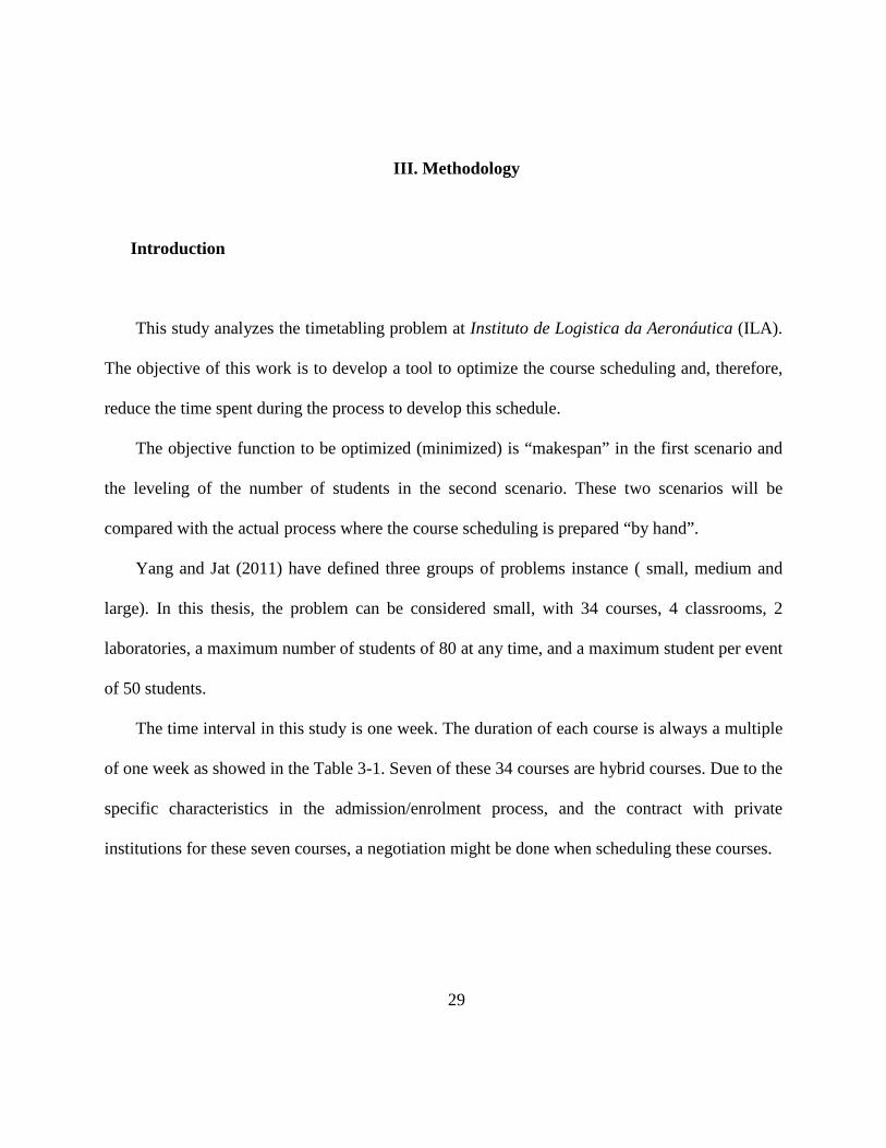
Yang and Jat (2011) have defined three groups of problems instance ( small, medium and

large). In this thesis, the problem can be considered small, with 34 courses, 4 classrooms, 2

laboratories, a maximum number of students of 80 at any time, and a maximum student per event

of 50 students.

The time interval in this study is one week. The duration of each course is always a multiple

of one week as showed in the Table 3-1. Seven of these 34 courses are hybrid courses. Due to the

specific characteristics in the admission/enrolment process, and the contract with private

institutions for these seven courses, a negotiation might be done when scheduling these courses.

30

course duration

(weeks) nº students (max)

type of course

caalf 1 20 in class

cac 2 30 in class

cacfo 1 20 in class

cadti 1 30 in class

cadti /2 1 30 in class

cambel 2 20 in class

capsa 3 10 in class

casup 2 30 in class

catcis 2 30 in class

cbmo 3 30 in class

ccnp 2 15 in class

cenm 2 30 in class

cfms 2 20 in class

cgps 2 30 in class

cgsup 3 30 in class

cidmat 2 30 in class

cimbe 2 20 in class

cins 3 15 in class

cneg 1 3 30 in class

cneg 2 3 30 in class

codmat 2 20 in class

cpac 2 30 in class

cpat 1 30 in class

cpnp 3 15 in class

cpoa 1 2 12 in class

cpoa 2 2 12 in class

cst 1 30 in class

cbmo (s) 1 40 hybrid

ceslog (s) 6 30 hybrid

cfacc 1 (s) 1 42 hybrid

cfacc 2 (s) 1 42 hybrid

cima 1 (s) 1 42 hybrid

cima 2 (s) 1 42 hybrid Table 3-1 – courses scheduled for 2011

31

As previously mentioned, the actual process of course scheduling starts in August and

finishes in November, when the approval and publication of the document TCA37-11

(Aeronautic Command Table number 37-11) occurs. This process is based on a series of

meetings, normally one meeting per month during the planning period of two days of duration.

During these meetings, the demand for each course is discussed. This discussion can result in a

change in the number of students per course or the creation/deletion of others courses.

Each new alternative of the course schedule is analyzed with the existing constraints by

hand. Therefore this process is arduous and time consuming. As the actual process is not based in

any stated objective function, a large number of alternatives are possible, personal feelings are

often predominant, and conflicts of opinions can occur.

The constraints are important for the final course schedule, since no violation is allowed.

These constraints include the total number of student per week, the number of students allowed

per room, number of students allowed per laboratory, and the continuity of the course (no

preemption is allowed).

Problem formulation

According to Tripathy (1984) , the process of producing a timetabling has three main

phases:

(i) Deciding the group of students who are to attend a particular subject.

(ii) Specifying the facilities required by the subject.

(iii) Determining when each subject is to take place.

32

The first two phases involve certain major decisions to be taken by the academic staff and

the administrator. These often do not follow any specific mathematical rules and hence are done

manually. The first two phases, when completed, completely define the subjects, and these form

the data for use in the third phase.

Decision Variables

Given a predefined number of courses per year (n courses), the index i represents a

specific course in the model where i = 1,…, n . Each course i has a specific duration of weeks

(Ti) and a number of students (Ni).

The time interval in this problem is one week, because any course duration is a multiple

of one week. As the month of January is reserved for vacation, the week of carnival and the last

two weeks of the year are reserved due to holidays, the maximum number of weeks available are

45 (m). The index j represents each specific week available for one course. Therefore j = 1, … ,

m or j = 1, … , 45 in this case.

Based on these definitions, the decision variable for this problem can be expressed as x11

… xij is a binary number equal to one if the course i is allocated at time j and 0 otherwise.

Another decision variable in this problem is the laboratory (l) to be used. As ILA has two

laboratories, the index k is used to designate if the laboratory to be used is laboratory 1 or

laboratory 2. Therefore, the variable lijk is a binary variable that is equal to 1 when the laboratory

k is used for course i at time j, and 0 otherwise.

The last decision variable in this problem is the room to be used (r). As ILA has four

rooms, the index w is used to define if the room to be used is the room 1, 2, 3 or room 4.

33

Therefore the variable rijw is a binary variable that’s equal to 1 when the room w is used for

course i at time j, and 0 otherwise.

Constraints

Based on the decision variables, the constraints in this problem can be developed.

The first constraint considered is related with the objective function Cmax. Cmax represents

the maximum number of weeks used in the schedule. Minimizing the maximum completing time

of all activities, Cmax, is a classic scheduling objective. It processes the classes as quickly as

possible, leaving available capacity for others events. Therefore, when any course is placed at

time j, Cmax have to be greater than or equal to the week j. This constraint is expressed by;

𝐶𝑚𝑎𝑥 ≥ 𝑥𝑖𝑗 ∗ 𝑗 ⦡𝑖 , ⦡𝑗

The second constraint considered is the hotel capacity. Due to the capacity of the hotel, the

total number of students per week should be no more than 80 students. Therefore, for each

timeslot j , the sum of students should be less than or equal to 80. Each course, within the n

courses, has a defined number of student, therefore the parameter Ni represents the maximum

number of student for course i. When a course i is allocated at timeslot j (xij = 1) the sum of the

products xij . Ni must be less than 80. This constraint is expressed by :

∑ 𝑥𝑖𝑗 ∗ 𝑁𝑖 ≤ 80 ⦡𝑗𝑛𝑖=1 .

The third constraint considered is the laboratory capacity. As laboratory 1 has a limit of 18

students, the product lij1 * Ni must be less than or equal to 18, and the laboratory 2 has a limit of

34

33 students, therefore the product lij2 * Ni must be less than or equal to 33

∑ 𝑙𝑖𝑗1 ∗ 𝑁𝑖 ≤ 18 ⦡𝑗 , ∑ 𝑙𝑖𝑗2 ∗ 𝑁𝑖 ≤ 33𝑛𝑖=1 ⦡𝑗𝑛

𝑖=1 𝑙𝑎𝑏𝑜𝑟𝑎𝑡𝑜𝑟𝑦 𝑐𝑎𝑝𝑎𝑐𝑖𝑡𝑦.

Of course, at time j only one course must be taken for each laboratory (fourth constraint).

The binary variable lci indicates the necessity for the utilization of any laboratory for course i , is

expressed by

𝑥𝑖𝑗 ∗ 𝑙𝑐𝑖 = � 𝑙𝑖𝑗𝑘2

𝑘=1 ∀𝑖 ,∀𝑗.

The fifth constraint considered is the room capacity. Each course needs a room even when

the laboratory is used. As room 1 has a limit of 35 students, the product rij1 * Ni must be less than

or equal to 35, and the others rooms has a limit of 42 for room 2, 33 for room 3 and only 25 for

room 4, expressed by:

�𝑟𝑖𝑗1 ∗ 𝑁𝑖 ≤ 35 ⦡𝑗 , 𝑛

𝑖=1

�𝑟𝑖𝑗2 ∗ 𝑁𝑖 ≤ 42 ⦡𝑗 , 𝑐𝑎𝑝𝑎𝑐𝑖𝑡𝑦 𝑜𝑓 𝑐𝑙𝑎𝑠𝑠𝑟𝑜𝑜𝑚 1 𝑎𝑛𝑑 2𝑛

𝑖=1

�𝑟𝑖𝑗3 ∗ 𝑁𝑖 ≤ 33 ⦡𝑗𝑛

𝑖=1

, �𝑟𝑖𝑗4 ∗ 𝑁𝑖 ≤ 25 ⦡𝑗𝑛

𝑖=1

𝑐𝑎𝑝𝑎𝑐𝑖𝑡𝑦 𝑜𝑓 𝑐𝑙𝑎𝑠𝑠𝑟𝑜𝑜𝑚 3 𝑎𝑛𝑑 4

Of course, at time j only one course may be taken for each room (sixth constraint), and the

course must be taken in one classroom (seventh constraint).

�𝑟𝑖𝑗𝑤

𝑛

𝑖=1

≤ 1 ⦡𝑗 , ⦡𝑤

𝑥𝑖𝑗 = ∑ 𝑟𝑖𝑗𝑤4𝑤=1 ⦡𝑖 , ⦡𝑗

The eighth constraint is the duration of the course. The sum of the weeks scheduled for one

course must be equal to the total duration of the course according to the TCA 37-11.

35

�𝑥𝑖𝑗 = 𝑇𝑖 ∀𝑖

𝑚

𝑗=1

The last constraint is the continuity of the course. Once a course has started, it is not possible

to interrupt the course to be finish later.

In this thesis, there is no constraints related with the sequence of the courses, and no

precedence exists between these courses.

𝑁𝑖 ∗ 𝑥𝑖𝑗 − 𝑁𝑖 ∗ 𝑥𝑖,𝑗+1 + � 𝑥𝑖𝑗 ∗ 𝑁𝑖 ≤ 𝑁𝑖 ∀𝑖𝑛

𝑗=𝑖+2

Objective function

In this work, there are two different approaches and therefore two different objective

functions. The first approach is to minimize the “makespan” or Cmax . With this approach, the

objective is to allow free timeslots without courses that could be used for the others activities as

evaluation and planning of courses or seminars, meetings, lectures and so forth.

Another approach is to minimize the maximum number of students per week. With this

approach the idea is to have a constant utilization of resources at a minimum required level.

When another activity is placed at any time, there is a minimum interference between this extra-

activity and the courses and, therefore, minimizing the problems with resources available.

Decision variables:

Let xij (binary) = 1 if course i is placed at time j . Let rijw (binary) =1 if room w is placed for

course i at time j. Let lijk (binary) =1 if lab k is placed at time j for course i.

Ci = 1 if course i needs a lab. Ni = number students in course i. Ti= duration of course i.

36

Mathematical formulation

In the first instance ( makespan) the problem is formulated as:

Minimize Cmax

Subject to:

𝐶𝑚𝑎𝑥 ≥ 𝑥𝑖𝑗 ∗ 𝑗 ⦡𝑖 , ⦡𝑗

∑ 𝑥ì𝑗 ∗ 𝑁𝑖 ≤ 80 ⦡𝑗𝑛𝑖=1 hotel capacity

�𝑙𝑖𝑗1 ∗ 𝑁𝑖 ≤ 18 ⦡𝑗 , �𝑙𝑖𝑗2 ∗ 𝑁𝑖 ≤ 33𝑛

𝑖=1

⦡𝑗𝑛

𝑖=1

𝑙𝑎𝑏𝑜𝑟𝑎𝑡𝑜𝑟𝑦 𝑐𝑎𝑝𝑎𝑐𝑖𝑡𝑦

�𝑟𝑖𝑗1 ∗ 𝑁𝑖 ≤ 35 ⦡𝑗 , 𝑛

𝑖=1

�𝑟𝑖𝑗2 ∗ 𝑁𝑖 ≤ 42 ⦡𝑗 , 𝑐𝑎𝑝𝑎𝑐𝑖𝑡𝑦 𝑜𝑓 𝑐𝑙𝑎𝑠𝑠𝑟𝑜𝑜𝑚 1 𝑎𝑛𝑑 2𝑛

𝑖=1

�𝑟𝑖𝑗3 ∗ 𝑁𝑖 ≤ 33 ⦡𝑗𝑛

𝑖=1

, �𝑟𝑖𝑗4 ∗ 𝑁𝑖 ≤ 25 ⦡𝑗𝑛

𝑖=1

𝑐𝑎𝑝𝑎𝑐𝑖𝑡𝑦 𝑜𝑓 𝑐𝑙𝑎𝑠𝑠𝑟𝑜𝑜𝑚 3 𝑎𝑛𝑑 4

∑ 𝑥𝑖𝑗 = 𝑇𝑖 ∀𝑖 𝑚𝑗=1 Duration of the courses

�𝑟𝑖𝑗𝑤

𝑛

𝑖=1

≤ 1 ⦡𝑗 , ⦡𝑤 𝑜𝑛𝑒 𝑐𝑜𝑢𝑟𝑠𝑒 𝑝𝑒𝑟 𝑐𝑙𝑎𝑠𝑠𝑟𝑜𝑜𝑚

𝑥𝑖𝑗 ∗ 𝑙𝑐𝑖 = ∑ 𝑙𝑖𝑗𝑘2𝑘=1 ∀𝑖 ,∀𝑗 utilization of laboratory when necessary

𝑥𝑖𝑗 = ∑ 𝑟𝑖𝑗𝑤4𝑤=1 ⦡𝑖 , ⦡𝑗 utilization of room

𝑁𝑖 ∗ 𝑥𝑖𝑗 − 𝑁𝑖 ∗ 𝑥𝑖,𝑗+1 + ∑ 𝑥𝑖𝑗 ∗ 𝑁𝑖 ≤ 𝑁𝑖 ∀𝑖𝑛𝑗=𝑖+2 no splitting courses

xij , rijw, lijk are binary ⦡𝑖 , ⦡𝑗, ⦡𝑤 , ⦡𝑘

In the second instance (minimum number of students per week) the problem is

formulated as:

37

Minimize : Amax

Subject to:

�𝑥𝑖𝑗 ∗ 𝑁𝑖 ≤ 𝐴𝑚𝑎𝑥𝑛

𝑗=1

�𝑥𝑖𝑗 ∗ 𝑁𝑖 ≤ 80 ⦡𝑗𝑛

𝑖=1

�𝑙𝑖𝑗1 ∗ 𝑁𝑖 ≤ 18 ⦡𝑗 , �𝑙𝑖𝑗2 ∗ 𝑁𝑖 ≤ 33𝑛

𝑖=1

⦡𝑗𝑛

𝑖=1

�𝑟𝑖𝑗1 ∗ 𝑁𝑖 ≤ 35 ⦡𝑗 , 𝑛

𝑖=1

�𝑟𝑖𝑗2 ∗ 𝑁𝑖 ≤ 42 ⦡𝑗 , 𝑛

𝑖=1

�𝑟𝑖𝑗3 ∗ 𝑁𝑖 ≤ 33 ⦡𝑗𝑛

𝑖=1

, �𝑟𝑖𝑗4 ∗ 𝑁𝑖 ≤ 25 ⦡𝑗𝑛

𝑖=1

�𝑥𝑖𝑗 = 𝑇𝑖 ∀𝑖

𝑚

𝑗=1

�𝑟𝑖𝑗𝑤

34

𝑖=1

≤ 1 ⦡𝑗 , ⦡𝑤

𝑥𝑖𝑗 ∗ 𝑙𝑐𝑖 = � 𝑙𝑖𝑗𝑘2

𝑘=1 ∀𝑖 ,∀𝑗

𝑥𝑖𝑗 = � 𝑟𝑖𝑗𝑤

4

𝑤=1

⦡𝑖 , ⦡𝑗

𝑁𝑖 ∗ 𝑥𝑖𝑗 − 𝑁𝑖 ∗ 𝑥𝑖,𝑗+1 + ∑ 𝑥𝑖𝑗 ∗ 𝑁𝑖 ≤ 𝑁𝑖 ∀𝑖𝑛𝑗=𝑖+2

xij , rijw, lijk are binary ⦡𝑖 , ⦡𝑗, ⦡𝑤 , ⦡𝑘

38

Methodology Issues

While there are potentially many factors to consider when scheduling activities, as

courses, here the hotel capacity, room availability, and laboratory availability are considered.

Considering the year of 2010, 34 courses were scheduled to be done at ILA. The schedule

generated by hand is compared with the solutions presented in this work.

In this model, as there are 34 courses and 40 time slots, resulting in 1360 binaries

variables related with the courses.

The number of constraints in this problem is 40 for the hotel capacity, 40 for each room

(there are 4 rooms available), 40 for each laboratory (there are two laboratories), 34 to constrain

the duration of the course, 1360 constraints to force the use of one room, 1360 constraints to

force the use of laboratory when necessary and the last constraint type has 1292 constraints to

avoid any splitting between the beginning and the end of course. Therefore the total number of

constraint is 4326. While large, this model can be solved to optimality.

39

Investigation Design

The makespan problem was solved to find the optimal solution using the Branch and

Bound algorithm. The software used for this purpose was LINGO from Lingo Systems Inc. using

the default parameters. The solution for the makespan objective function was 23 weeks with a

total time to find the optimal solution was 72 hours using a computer with 4 Gb RAM,and 2.7

GHz processor . The solution is showed in the Table 3-2. A Gantt Chart, using the software

Gantt project, is available for this solution in appendix B.

course duration Weeks scheduled for the course

course duration Weeks scheduled for the course

1 1 18 18 3 13 , 14 and 15 2 2 20 , 21 19 3 3 , 4 and 5 3 1 3 20 3 1 , 2 and 3 4 1 18 21 2 18 , and 19 5 1 15 22 2 11 and 12 6 2 13 and 14 23 1 11 7 3 7 , 8 and 9 24 3 12 , 13 and 14 8 2 7 and 8 25 2 4 and 5 9 2 16 and 17 26 2 19 and 20

10 3 20 , 21 and 22 27 1 10 11 2 16 and 17 28 1 9 12 2 6 and 7 29 6 12,13,14,15,16 and

13 2 21 and 22 30 1 23 14 2 22 and 23 31 1 19 15 3 8 , 9 and 10 32 1 1 16 2 4 and 5 33 1 2 17 2 10 and 11 34 1 6 Table 3-2 – solution for makespan approach

The utilization of the hotel is showed in the Figure 3-1. Figure 3-1 shows that hotel

utilization is close to or at capacity in these first 23 weeks if the Cmax schedule is used.

40

Figure 3-1 – Hotel utilization based on the previous solution.

The utilization of the classrooms is often low, and even when there is 4 rooms in use with

courses in any week, these courses had fewer students due the hotel capacity. This fact results in

available seats in the classrooms. The number of rooms utilized in this solution is showed below

in Figure 3-2.

Figure 3-2 – Classroom utilization based on the previous solution.

0

10

20

30

40

50

60

70

80

90 total students per week

0

1

2

3

4

1 3 5 7 9 11 13 15 17 19 21 23 25 27 29 31 33 35 37 39 41 43

number of rooms utilized

41

The laboratory utilization was very low, with the utilization often zero; the slack was

always greater than 50% of the capacity.

This solution seems to show a large excess of capacity and might allow more courses

than the plan for 2011. However, a high concentration of courses could result in problems with

others resources not considered in this thesis. For example, the human resource availability can

be a constraint that does not allow this type of approach. The formulation for availability of

human resource is complex and is out of scope for this work. Another consideration would be

having time to undertake required maintenance. If used to capacity, there is no “stand by”

resources for critical repair or scheduled maintenance.

These results illustrate the hotel capacity is the main constraint in this compressed

schedule problem. Increasing the room capacity, either by increasing the number of room or the

students per classroom, would not dramatically change the result due the hotel limit.

For the second instance, the objective is to spread the courses uniformly within a certain

number of weeks. Initially the problem was solved for 40 weeks, but in this case there is no

interruption within the period with courses, that means, the 40 weeks are continually scheduled

for courses. The optimal solution was achieved after 1 hour and 45 minutes. The solution is

shown in the Table 3-3, but this result will not be used in further analysis, due the fact that the

carnival is a period that must be free of courses, and this fact is not represented in this solution.

A Gantt chart for this solution is in appendix C. This result shows that only a maximum of two

classrooms were necessary and only one laboratory was necessary. Therefore a reduction on the

42

number of constraints could be applied, reducing the number of classrooms and laboratories in

the model. This reduction in the number of constraints was applied in further investigation.

course duration Weeks scheduled course duration Weeks scheduled

1 1 38 18 3 24,25 and 26 2 2 7 and 8 19 3 27,28 and 29 3 1 37 20 3 30,31 and 32 4 1 9 21 2 29 and 30 5 1 10 22 2 39 and 40 6 2 35 and 36 23 1 39 7 3 14, 15 and 16 24 3 21,22 and 23 8 2 11 and 12 25 2 19 and 20 9 2 13 and 14 26 2 17 and 18

10 3 15, 16, and 17 27 1 40 11 2 27 and 28 28 1 6 12 2 18 and 19 29 6 33,34,35,36,37 and 38 13 2 33 and 34 30 1 1 14 2 20 and 21 31 1 2 15 3 22, 23 and 24 32 1 3 16 2 25 and 26 33 1 4 17 2 31 and 32 34 1 5 Table 3-3 – solution for second instance

The utilization of the hotel is showed in Figure 3-3, where it is possible to provide a

distribution of students across the year.

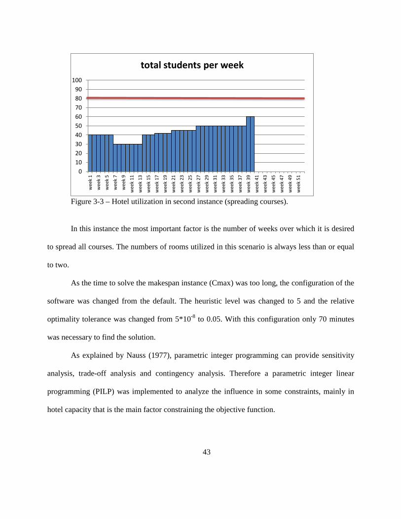
43

Figure 3-3 – Hotel utilization in second instance (spreading courses).

In this instance the most important factor is the number of weeks over which it is desired

to spread all courses. The numbers of rooms utilized in this scenario is always less than or equal

to two.

As the time to solve the makespan instance (Cmax) was too long, the configuration of the

software was changed from the default. The heuristic level was changed to 5 and the relative

optimality tolerance was changed from 5*10-8 to 0.05. With this configuration only 70 minutes

was necessary to find the solution.

As explained by Nauss (1977), parametric integer programming can provide sensitivity

analysis, trade-off analysis and contingency analysis. Therefore a parametric integer linear

programming (PILP) was implemented to analyze the influence in some constraints, mainly in

hotel capacity that is the main factor constraining the objective function.

0 10 20 30 40 50 60 70 80 90

100 w

eek

1 w

eek

3 w

eek

5 w

eek

7 w

eek

9 w

eek

11

wee

k 13

w

eek

15

wee

k 17

w

eek

19

wee

k 21

w

eek

23

wee

k 25

w

eek

27

wee

k 29

w

eek

31

wee

k 33

w

eek

35

wee

k 37

w

eek

39

wee

k 41

w

eek

43

wee

k 45

w

eek

47

wee

k 49

w

eek

51

total students per week

44

In this work, five scenarios were created to analyze the influence of the expansion of

hotel capacity. There are four students for each room available in the hotel and each new

scenario represents one new room. These new rooms are represented by the variable g, where g

is the number of new rooms.

For the makespan instance the PILP used is:

For g = 0,1,2,3 and 4 solve:

Minimize Cmax;

Subject to:

�𝑥𝑖𝑗 ∗ 𝑁𝑖 ≤ 80 + 𝑔 ∗ 4𝑛

𝑖=1

While others constraints remain the same.

For the second instance where the objective is to spread the courses, it is important to

know the influence of the weeks reserved for special events. In these weeks no courses are

scheduled in this work. Therefore, when a week is reserved for special events, the variable xij

must be equal to zero for any course.

In the second instance five scenarios were created. One scenario has just the week of

carnival without courses, and the others scenarios has others weeks without courses in addition

to carnival week. For each scenario the weeks without a course varies from 1 to 7, and when is

possible, preferably at the end of the quarter.

The PILP can support a comparison of results and analysis in the next chapter.

45

IV. Analysis and Results

Context of Model Results

This section details a comparative analysis of the actual timetable using the method

developed in this thesis. The first comparison is related with the “makespan” approach, where

the objective function is to concentrate the courses to allow free periods for others activities.

The second approach is the spread of the courses leveling resources requirements, Various

scenarios are compared. Based on the results founded in the second approach, the possibility of

increasing the number of students was analyzed.

Analysis of the first approach

The first approach, minimizing makespan, was to concentrate all the courses within a period

of time. In scheduling theory minimizing makespan attempts to finish all available jobs (courses

in this case) as soon as possible to free up resources for other needs. Therefore, during the period

with courses, there is no opportunity to perform any other activity or special events. All available

resource, including human resource, should be dedicated to courses in this compressed period

period. These others activities (special events) could occur only in the period without courses;

all of ILA’s resources should be available for these special events. Therefore, no interferences

could occurs between these activities. In addition, the block of “free time”(unscheduled choses)

could be available for other activities.

From the result showed in Table 3-2, only 23 weeks are necessary to schedule all the thirty

six courses offered during the year of 2011. This result shows that less than half of the year is

necessary to execute the courses based in the constraints mentioned in the methodology.

46

However, others resources not included in the model could not execute all these courses in a

short period of time of 23 weeks. For example, the human resources would not be sufficient in

this scenario. The availability of personnel is outside of scope in this work. Another example is

the maintenance capacity to support the courses, including the maintenance of the facilities and

computers. For this reason this approach is not considered practical.

The constraint without slack, in this compressed solution, is the hotel capacity, while the

others constraints still have excess capacity. Even in this compressed scenario, there is a excess

of classrooms, laboratories, and seats available.

Based in this result it was possible to investigate the increasing in hotel capacity as defined

in the PILP described in the chapter III. With a capacity of 92 students in the hotel, it would be

possible to reduce the “makespan” of the year’s courses to 20 weeks. Figure 4-1 shows the

increase the utilization of classrooms to 93%. However, this result is also not practical and no

further analysis is conducted on this issue.

Figure 4-1 – Classrooms utilization in first instance with hotel capacity for 92 students.

0

1

2

3

4

5

w 1

w 3

w 5

w 7

w 9

w 11

w 13

w 15

w 17

w 19

w 21

w 23

w 25

w 27

w 29

w 31

w 33

w 35

w 37

w 39

w 41

w 43

w 45

w 47

w 49

w 51

number of classrooms utilized with hotel capacity for 92 students

47

If a compressed schedule was possible and/or more space was available at the hotel it would

be possible to increase the number of courses offered. Considering the same distribution of the

number of students per course, the number of courses could be duplicated without any violation

of any constraint considered in the model. Again, however, as mentioned before, there are

considerations about others constraints, and the approach to spread the courses within some

predefined period of time seems more reasonable.

Analysis of the second approach

In this approach the courses are distributed during the year to smooth the utilization of the

resources while reserving a few weeks for special events. The unique scenario where there is

superimposition of courses and special events, is the last scenario which all courses are

distributed within the 45 weeks available.

In this approach five scenarios were created, based on the PILP described previously, to

compare with the current schedule. The month of January does not have courses because it is the

traditional month for vacations. The week for carnival and Christmas are also not scheduled for

courses. Given these restrictions, the first scenario is 38 weeks for courses and 7 weeks for

special events; the second scenario is 40 weeks for courses and 5 weeks for special events; the

third scenario is 42 weeks for courses and 3 weeks reserved for special events; the fourth

scenario is 44 weeks for courses and 1 week for special events; and the last scenario has all 45

weeks with courses without any week specifically reserved for special event. In any scenario, the

48

weeks without courses are divided between the four quarters and placed at the end of the quarter,

except in the last scenario where all 45 weeks available is planned for courses.

Figure 4-2 shows the number of students per week based on the approved schedule in the

current TCA 37-11 and the number of classrooms used. In this schedule, the number of students

per week varies from 15 to 80 ( avg 45, sd 24), with 7 weeks without courses. These 7 weeks are

the traditional January, Christmas and carnival holidays. There are 10 weeks when only 1

classroom is used, 15 weeks when 2 classrooms are used and 13 weeks with 3 classrooms.

49

Figure 4-2 – Hotel utilization based on the courses scheduled for 2011 (TCA 37-11/2010)

Figure 4-3 shows the profile of students per week with 7 weeks reserved for special events.

In this scenario the number of students per week varies from 30 to 60 (avg 45, std 7.7) when

there is not a free week. In this configuration there is 19 weeks utilizing only one classroom and

29 weeks utilizing 2 classrooms. The total number of students taught is 1718 during the year.

0 10 20 30 40 50 60 70 80 90

wee

k 1

wee

k 3

wee

k 5

wee

k 7

wee

k 9

wee

k 11

w

eek

13

wee

k 15

w

eek

17

wee

k 19

w

eek

21

wee

k 23

w

eek

25

wee

k 27

w

eek

29

wee

k 31

w

eek

33

wee

k 35

w

eek

37

wee

k 39

w

eek

41

wee

k 43

w

eek

45

wee

k 47

w

eek

49

wee

k 51

Number of students per week based on approved schedule in TCA 37-11 Number of students per week based on approved schedule in TCA 37-11

0

1

2

3

4

wee

k 1

wee

k 3

wee

k 5

wee

k 7

wee

k 9

wee

k 11

w

eek

13

wee

k 15

w

eek

17

wee

k 19

w

eek

21

wee

k 23

w

eek

25

wee

k 27

w

eek

29

wee

k 31

w

eek

33

wee

k 35

w

eek

37

wee

k 39

w

eek

41

wee

k 43

w

eek

45

wee

k 47

w

eek

49

wee

k 51

Number of classroom utilized based on approved schedule in TCA 37-11

50

This alternative shows a solution with a smoother utilization of resources than the approved

schedule. The standard deviation of the number of students is 24 in the approved TCA 37-11 and

just 7.7 in this alternative.

The advantage in this alternative is to plan 7 weeks for special events without conflicts with

courses, while the courses is distributed in the others weeks allowing more uniformly demand for

ILA resources.

Figure 4-3 – Hotel utilization with courses distributed within 38 weeks.

Figure 4-4 shows the number of students per week in the scenario with 3 weeks reserved for

special events. The number of students per week varies from 30 to 50 (avg 41, std 7.4). The

number of weeks with one classroom used is seventeen and the number of weeks using two

classrooms is 25. Compared with the first scenario which has 38 weeks for courses and 7 weeks

for special events, this alternative is significantly different at 5% level (p-value=0.014).

0 10 20 30 40 50 60 70 80 90

100

wee

k 1

wee

k 3

wee

k 5

wee

k 7

wee

k 9

wee

k 11

w

eek

13

wee

k 15

w

eek

17

wee

k 19

w

eek

21

wee

k 23

w

eek

25

wee

k 27

w

eek

29

wee

k 31

w

eek

33

wee

k 35

w

eek

37

wee

k 39

w

eek

41

wee

k 43

w

eek

45

wee

k 47

w

eek

49

wee

k 51

Total students per week(38w) carnival+ 7 weeks free -1718 stud.

51

Therefore, the null hypothesis H0: the means in both scenarios are equal, should be reject at a

5% potential error.

Figure 4-4 – Hotel utilization with courses distributed within 42 weeks. The last scenario in this approach, without free weeks reserved for special events, results in a

solution smoother than the others. The number of students per week varies from 30 to 50 (avg

38, std 6.5). This result is significantly different from the first scenario with 38 weeks at 5% level

, but is not significantly different from the second scenario (p-value= 0.07). The number of

weeks utilizing only 1 classroom is 22, therefore there is 23 weeks using 2 classrooms. But in

this case, when a special event must be placed, there will be potential conflicts with courses in

the same week. In addition, any attendees for the special event may need to compete for rooms at

the hotel with the assigned students. Figure 4-5 shows the hotel utilization in this last scenario.

0 10 20 30 40 50 60 70 80 90

100

wee

k 1

wee

k 3

wee

k 5

wee

k 7

wee

k 9

wee

k 11

w

eek

13

wee

k 15

w

eek

17

wee

k 19

w

eek

21

wee

k 23

w

eek

25

wee

k 27

w

eek

29

wee

k 31

w

eek

33

wee

k 35

w

eek

37

wee

k 39

w

eek

41

wee

k 43

w

eek

45

wee

k 47

w

eek

49

wee

k 51

Total students per week(42w) carnival+ 3 weeks free

52

Figure 4-5 – Hotel utilization with courses distributed within 45 weeks.

The utilization of the model with only two classrooms and one laboratory was important

to reduce the executing times. The higher processing time was found in the last scenario. In this

scenario was necessary 5 hours and 31 minutes to run the model, even running the model with

only two classrooms and one laboratory.

The period without courses could be used not only for special events, but for others activities

such as course evaluation with customers, research, support for process improvement in the Air

Force or support for Strategic Acquisition Process like the FX-2 program ( acquisition of new

fighters for Brazilian Air Force). These activities are currently performed only when required by

the high management level for important projects, and could be performed more frequently with

this approach to spread the courses.

0

10

20

30

40

50

60

70

80

90

100 w

eek

1 w

eek

3 w

eek

5 w

eek

7 w

eek

9 w

eek

11

wee

k 13

w

eek

15

wee

k 17

w

eek

19

wee

k 21

w

eek

23

wee

k 25

w

eek

27

wee

k 29

w

eek

31

wee

k 33

w

eek

35

wee

k 37

w

eek

39

wee

k 41

w

eek

43

wee

k 45

w

eek

47

wee

k 49

w

eek

51

Total students per week(45w) only carnival, January and christmas without courses

53

Analysis of the number of students trained per year

The mathematical model used allows the visualization of the classroom to be used in each

course. It is also then possible to analyses the full utilization of the classroom capacity while

respecting the others constraints.

In the actual process without any optimization tool, only the schedule of the courses has

been done, and the final document (TCA 37-11) does not provide any information about the

classroom to be used. Therefore, normally for courses with higher demands only 30 students are

planned.

The utilization of optimization tools allows the visualization of the possibility to increase the

number of students for some courses. The largest room available at ILA has capacity for 42

students while the second largest has capacity for 35. Therefore, some courses could increase the

number of students taught to satisfy the demand without any increase in the number of courses or

direct cost with instructors that could be a new constraint for the problem. There would,

however, be a potential indirect cost to the instructor who could have larger courses. Therefore,

for each scenario presented in the second instance the increase of students is analyzed.

In the case of spreading the courses within 38 weeks with 7 weeks free for special events, it

is possible to increase the total number of students per year from 1718 to 2035 or an increase

equivalent of 18%. Figure 4-6 shows the hotel utilization in this situation.

54

Figure 4-6 – Hotel utilization with courses distributed within 38 weeks with full utilization in

room.

In the case where only 3 weeks per year are reserved for special events, the number of total

students per year could be increased to 2105. This shows a potential of 22% more students per

year than the actual schedule. Again, this alternative is based on the capacity of the classroom,

laboratory and the hotel; the demand for each of these courses could be lower than the estimated

in this work. A maximum of two classrooms and one laboratory were necessary.

While more students are processed, there is less flexibility for others events because only

three weeks are planned for these events. Figure 4-7 shows the hotel utilization in this case.

0 10 20 30 40 50 60 70 80 90

100 w

eek

1

wee

k 3

wee

k 5

wee

k 7

wee

k 9

wee

k 11

wee

k 13

wee

k 15

wee

k 17

wee

k 19

wee

k 21

wee

k 23

wee

k 25

wee

k 27

wee

k 29

wee

k 31

wee

k 33

wee

k 35

wee

k 37

wee

k 39

wee

k 41

wee

k 43

wee

k 45

wee

k 47

wee

k 49

wee

k 51

total students per week(38w) carnival+ 7 weeks free - 2035 stud.

55

Figure 4-7 – Hotel utilization with courses distributed within 42 weeks with full utilization in

room.

In the extreme case with no week set aside for special events and all 45 weeks are used for

courses, it is possible to increase the total number of students per year from 1718 to 2166. That

represents an increase of 26%. Again, in this scenario there is no flexibility for others events.

There is always a conflict with courses when other event needs to be scheduled. Figure 4-8

exhibits the hotel utilization in this case.

0 10 20 30 40 50 60 70 80 90

100 w

eek

1

wee

k 3

wee

k 5

wee

k 7

wee

k 9

wee

k 11

wee

k 13

wee

k 15

wee

k 17

wee

k 19

wee

k 21

wee

k 23

wee

k 25

wee

k 27

wee

k 29

wee

k 31

wee

k 33

wee

k 35

wee

k 37

wee

k 39

wee

k 41

wee

k 43

wee

k 45

wee

k 47

wee

k 49

wee

k 51

total students per week(42w) carnival+ 3 weeks free - 2105 stud.

56

Figure 4-8 – Hotel utilization with courses distributed within 45 weeks with full utilization in room.

Based on these results, the makespan approach needs a more detailed model, including

others constraints as personal availability, reprographic service constraints, budget availability

and so forth. However, the second approach presents a feasible solution, when these others

resources not included in the model do not represent a constraint. This fact is easily proven once

the approved document TCA 37-11 has a similar approach, but presenting a large variation of

utilization.

In the actual configuration of courses, and students per course, there is 38 weeks with courses

and 7 weeks without courses besides the weeks reserved for Carnival, Christmas, and the January

month. The approved TCA 37-11 has higher variation in the utilization of resources (standard

deviation of 19.3 in number of students per week) than the solution of the mathematical model

with the same weeks for courses (standard deviation of 7.7 in the number of student per week).

0 10 20 30 40 50 60 70 80 90

100 w

eek

1

wee

k 3

wee

k 5

wee

k 7

wee

k 9

wee

k 11

wee

k 13

wee

k 15

wee

k 17

wee

k 19

wee

k 21

wee

k 23

wee

k 25

wee

k 27

wee

k 29

wee

k 31

wee

k 33

wee

k 35

wee

k 37

wee

k 39

wee

k 41

wee

k 43

wee

k 45

wee

k 47

wee

k 49

wee

k 51

total students per week(45w) only carnival- 2166 stud.

57

Due to this fact, the model presents the flexibility to select the desired week reserved for special

events where the variable xij may be fixed to zero. In the approved TCA 37-1, the weeks without

course are randomly distributed, only the carnival, Christmas and the January month are

previously defined. Thus, this approach could be the first step to use the mathematical model to

schedule courses for the next year.

The PILP provided different scenarios in each approach. Once only the second approach

presented a reasonable solution, this approach was investigated and served as basis for

recommendations in the last chapter of this thesis.

The possibility to increase the number of students taught is also feasible in this second

approach. The utilization of the hotel is under the limit, the number of courses per week is

always less than or equal to two, and the laboratory capacity is higher than the possible

utilization in each solution presented. Increasing the number of students per course should have

low impact on the cost of the courses, human resources, maintenance demand, and others

constraints not included in the model. The main restriction for increasing the students taught is

the capacity of the classrooms and the capacity of the laboratories. Therefore, it is possible to

evaluate an alternative to reduce the number of classroom, initially by one, while increasing the

capacity in the classrooms remained and expanding the laboratories. In order to perform this

evaluation, it is necessary to have more information about strategic goals and perspectives of

ILA and BAF in the long term, avoiding a future necessity to return back for the actual

configuration.

The tool does provide a guide for scheduling that can be relatively rapidly generated to

review and adjust to include unquantifiable goals. The analysis provides a base line which can

58

assist the discussion of the final schedule. Of course it may not be practicable to release more

airmen from duty for school in a given week. This would be a consideration for higher leadership

to consider.

59

V. Conclusions and Recommendations

The utilization of an optimization tool supports a faster process to develop scenarios for

scheduling the courses at ILA. The time spent for the formulation and for the implementation in

software was less than one day. After the implementation, the time spent by the computer for the

optimization was an average few hours with the selection of adequate parameters. Heuristic

approaches would be even fasting in generating schedules.

The initial approach to concentrate all the courses within a shortest time period was not a

good managerial solution due the fact that the courses were concentrated in a 23 week window.

This could result in high utilization, with limited slack in the system during these weeks.

However, others constraints such as human resources, maintenance capacity,

reprographic services and so forth, could make this solution impracticable. A complete analysis

considering all resources could be done to evaluate the practicable makespan. In this case, if

there is more weeks available than the necessary for special events, the excess capacity could be

used for others opportunities, for example be offered for others schools or even rented for private

institutions.

The approach to spread the courses within a time windows revealed a more interesting point

of view. The comparison of the results in this approach with the approved document based on the

actual process (manual) emphasized the possibility leveling the use of the resources.

Based on the decision by the top level leadership about the periods to be reserved for special

events, the spreading of the courses can avoid conflicts and defines a constant rhythm of

production.

60

Besides the fact that a more smooth utilization of resources could be possible, it is also

possible to increase the number of students taught in this approach. With a definition of the

classroom to be used at the end of the computational solution it is also possible to increase the

number of students that is planned to use any classroom. Classroom 2, for example, has capacity

for 42 students. However, due to the fact that in actual process the classroom to be used is not

defined, normally only 30 students is defined for each course. For 2011 only six courses were

planned with more than 30 students. The increase in the number of students per year could be at

least 18% using the technique of mathematical programming.

The recommendation for a process to be adopted, based on this work, is to use the second

approach, spreading the courses. However, the first step is to define the number of weeks to be

reserved for others events and when this should occurs. This information, additionally with the

courses definitions, could serve as base for a formulation and mathematical optimization in

several alternatives to serve as base in a meeting.

While such a planning tool will not supplant the final judgment of the leadership, it does

offer the opportunity to investigate various scenarios in a relatively expandable fashion. If

proposed requirements were available prior to the first scheduling meeting, a schedule could be

developed and presented to assist the initial gathering. In addition, the flexibility of mathematical

programming will allow a trained analyst to add requirements and constraints as they develop in

the planning process. The utilization of the proposed model might be a first step to more robust

scheduling planning.

61

Implementation

The implementation of a decision support tool should be carefully conducted. The approval

of the process should be conducted jointly by ILA and COMGAP.

ILA does not have any optimization software tool. The selection of an appropriate software is

important to achieve the desired results. Once it is decided to use a support tool to assist

managerial decisions such as the timetabling problem, some precautions should be taken.

The first step is to be sure that all participants understand the reasons for looking for a new

system and the expected outcome of the tool. An understanding of the applications and the

benefits of the tool could avoid any confusion with the results achieved. This tool can be used to

support not only course scheduling problems, but also to support managers in many others

decisions.

There are many optimization tools available in the market; LINDO, GAMs, Gurobi, and

Mozek among others. A detailed evaluation of the total cost of the software is important for the

proper selection and implementation of the tool. This cost must include upfront and ongoing

costs since pricing models vary among software vendors. Some vendors license their software by

installed workstation, named user, server and/or concurrent user. Costs associated with training,

manuals, upgrades, technical support among others must be included.

Since the decision of which tool to be used must include the ability of the vendor to provide

training, manuals, upgrades, technical support among others. Therefore, the acquisition and

implementation should be conducted by a small cross functional team. This selection and

implementation should follow a negotiated schedule. It is important to be able to conduct tests of

the software before purchases are made.

62

The majority of softwares allow the utilization of free period of test or a free demo with some

limitations. This fact should be explored to help the decision for the software selection.

After the selection and acquisition of the tool, training of the personnel involved,

documentation of manuals and other material in the library, and a test of the software, the

desired capability for the analysts should be determined.

Given the analysts are able to perform the utilization of the software, the inputs for the

process must be provided. In this case, for course scheduling, the definition of weeks available

for courses, period defined for special events, number of courses with specific number of

students and duration are the basic input for the problem. The possibility to increase the number

of students taught shows the necessity to evaluate the demand for the courses and their

importance for the Brazilian Air Force in order to prioritize which course could be planned for

classroom 2 with 42 students.

Some inputs can be different from the data used in this thesis. For example, one specific

course can be fixed for some time slot based on the knowledge of the managers, or a new

situation could imply in a precedence of one course related with another course.

Since these inputs are defined, the model could generate some alternatives for course

scheduling. These alternatives should be presented and discussed for the decision makers for

evaluation and some modifications can be necessary until the final approval.

It is important to emphasize this is support tool for decision makers. Therefore, it is

fundamental the knowledge and expertise of the managers to establish the appropriate schedule.

63

Recommendations for Future Research

The approach used in this work could also be used in different organizations at Brazilian Air

Force. The Brazilian Air Force has others organizations with the mission of education, training,

and improvements.

The Air Force Academy has three different undergraduate courses. Each course has four

years of duration and approximately 500 students. The BAF also has one high school, located in

Barbacena-MG with 700 students. The Air Force University has graduate courses and also could

consider mathematical programming for courses and exams scheduling.

Another possibility for further investigation is the further analysis of some heuristics,

particularly with some of these larger programs or considering more constraints. These might

include human resources, maintenance availability, reprographic services, budget constraints and

so forth. The utilization of heuristics could result in “good” solutions in shorter computational

time. Any heuristic has parameters that should be defined or analyzed in order to allow faster

convergence and/or shorter computational time. This fact demands deeper research and also

depend on the software and/or programming knowledge. However, the literature provides an

excellent starting point for deciding upon timetabling heuristics and parameters.

Further research, expanding this work, is possible to assist the educational leadership of the

Brazilian Air Force in their role of providing educational opportunities to develop airmen skills

and their abilities.

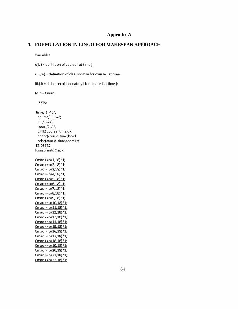
64

Appendix A

1. FORMULATION IN LINGO FOR MAKESPAN APPROACH

!variables

x(i,j) = definition of course i at time j

r(i,j,w) = definition of classroom w for course i at time j

l(i,j,l) = difinition of laboratory l for course i at time j;

Min = Cmax;

SETS:

time/ 1..40/; course/ 1..34/; lab/1..2/; room/1..4/; LINK( course, time): x; conec(course,time,lab):l; relat(course,time,room):r; ENDSETS !constraints Cmax;

Cmax >= x(1,18)*1; Cmax >= x(2,18)*1; Cmax >= x(3,18)*1; Cmax >= x(4,18)*1; Cmax >= x(5,18)*1; Cmax >= x(6,18)*1; Cmax >= x(7,18)*1; Cmax >= x(8,18)*1; Cmax >= x(9,18)*1; Cmax >= x(10,18)*1; Cmax >= x(11,18)*1; Cmax >= x(12,18)*1; Cmax >= x(13,18)*1; Cmax >= x(14,18)*1; Cmax >= x(15,18)*1; Cmax >= x(16,18)*1; Cmax >= x(17,18)*1; Cmax >= x(18,18)*1; Cmax >= x(19,18)*1; Cmax >= x(20,18)*1; Cmax >= x(21,18)*1; Cmax >= x(22,18)*1;

65

Cmax >= x(23,18)*1; Cmax >= x(24,18)*1; Cmax >= x(25,18)*1; Cmax >= x(26,18)*1; Cmax >= x(27,18)*1; Cmax >= x(28,18)*1; Cmax >= x(29,18)*1; Cmax >= x(30,18)*1; Cmax >= x(31,18)*1; Cmax >= x(32,18)*1; Cmax >= x(33,18)*1; Cmax >= x(34,18)*1;

…

Cmax >= x(1,40)*40; Cmax >= x(2,40)*40; Cmax >= x(3,40)*40; Cmax >= x(4,40)*40; Cmax >= x(5,40)*40; Cmax >= x(6,40)*40; Cmax >= x(7,40)*40; Cmax >= x(8,40)*40; Cmax >= x(9,40)*40; Cmax >= x(10,40)*40; Cmax >= x(11,40)*40; Cmax >= x(12,40)*40; Cmax >= x(13,40)*40; Cmax >= x(14,40)*40; Cmax >= x(15,40)*40; Cmax >= x(16,40)*40; Cmax >= x(17,40)*40; Cmax >= x(18,40)*40; Cmax >= x(19,40)*40; Cmax >= x(20,40)*40; Cmax >= x(21,40)*40; Cmax >= x(22,40)*40; Cmax >= x(23,40)*40; Cmax >= x(24,40)*40; Cmax >= x(25,40)*40; Cmax >= x(26,40)*40; Cmax >= x(27,40)*40; Cmax >= x(28,40)*40; Cmax >= x(29,40)*40; Cmax >= x(30,40)*40; Cmax >= x(31,40)*40; Cmax >= x(32,40)*40; Cmax >= x(33,40)*40; Cmax >= x(34,40)*40;

66

!considered 40 weeks enough - constraint hotel capacity 80;

X(1,1)*20+x(2,1)*30+x(3,1)*20+x(4,1)*30+x(5,1)*30+x(6,1)*20+x(7,1)*10+x(8,1)*30+x(9,1)*30+x(10,1)*30+x(11,1)*15+x(12,1)*30+x(13,1)*20+x(14,1)*30+x(15,1)*30+x(16,1)*30+x(17,1)*20+x(18,1)*15+x(19,1)*30+x(20,1)*30+x(21,1)*20+x(22,1)*30+x(23,1)*30+x(24,1)*15+x(25,1)*12+x(26,1)*12+x(27,1)*30+x(28,1)*40+x(29,1)*30+x(30,1)*42+x(31,1)*42+x(32,1)*42+x(33,1)*42+x(34,1)*42<=80;

…

X(1,40)*20+x(2,40)*30+x(3,40)*20+x(4,40)*30+x(5,40)*30+x(6,40)*20+x(7,40)*10+x(8,40)*30+x(9,40)*30+x(10,40)*30+x(11,40)*15+x(12,40)*30+x(13,40)*20+x(14,40)*30+x(15,40)*30+x(16,40)*30+x(17,40)*20+x(18,40)*15+x(19,40)*30+x(20,40)*30+x(21,40)*20+x(22,40)*30+x(23,40)*30+x(24,40)*15+x(25,40)*12+x(26,40)*12+x(27,40)*30+x(28,40)*40+x(29,40)*30+x(30,40)*42+x(31,40)*42+x(32,40)*42+x(33,40)*42+x(34,40)*42<=80;

!duration of courses;

x(1,1)+x(1,2)+x(1,3)+x(1,4)+x(1,5)+x(1,6)+x(1,7)+x(1,8)+x(1,9)+x(1,10)+x(1,11)+x(1,12)+x(1,13)+x(1,14)+x(1,15)+x(1,16)+x(1,17)+x(1,18)+x(1,19)+x(1,20)+x(1,21)+x(1,22)+x(1,23)+x(1,24)+x(1,25)+x(1,26) +x(1,27)+x(1,28)+x(1,29)+x(1,30)+x(1,31)+x(1,32)+x(1,33)+x(1,34)+x(1,35)+x(1,40) +x(1,37)+x(1,38) +x(1,39)+x(1,40)= 1;

…

X(34,1)+x(34,2)+x(34,3)+x(34,4)+x(34,5)+x(34,6)+x(34,7)+x(34,8)+x(34,9)+x(34,10)+x(34,11)+x(34,12)+x(34,13)+x(34,14)+x(34,15)+x(34,16)+x(34,17)+x(34,18)+x(34,19)+x(34,20)+x(34,21)+x(34,22)+x(34,23)+x(34,24)+x(34,25)+x(34,26) +x(34,27)+x(34,28)+x(34,29)+x(34,30) +x(34,31)+x(34,32)+x(34,33)+ x(34,34)+x(34,35)+x(34,40) +x(1,37)+x(1,38) +x(1,39)+x(1,40)= 1;

!laboratory 1 capacity;

l(1,1,1)*20+l(2,1,1)*30+l(3,1,1)*20+l(4,1,1)*30+l(5,1,1)*30+l(6,1,1)*20+l(7,1,1)*10+l(8,1,1)*30+l(9,1,1)*30+l(10,1,1)*30+l(11,1,1)*15+l(12,1,1)*30+l(13,1,1)*20+l(14,1,1)*30+l(15,1,1)*30+l(16,1,1)*30+l(17,1,1)*20+l(18,1,1)*15+l(19,1,1)*30+l(20,1,1)*30+l(21,1,1)*20+l(22,1,1)*30+l(23,1,1)*30+l(24,1,1)*15+l(25,1,1)*12+l(26,1,1)*12+l(27,1,1)*30+l(28,1,1)*40+l(29,1,1)*30+l(30,1,1)*42+l(31,1,1)*42+l(32,1,1)*42+l(33,1,1)*42+l(34,1,1)*42<=18;

…

L(1,40,1)*20+l(2,40,1)*30+l(3,40,1)*20+l(4,40,1)*30+l(5,40,1)*30+l(6,40,1)*20+l(7,40,1)+l(8,40,1)*30+l(9,40,1)*30+l(10,40,1)*30+l(11,40,1)*15+l(12,40,1)*30+l(13,40,1)*20+l(14,40,1)*30+l(15,40,1)*30+l(16,40,1)*30+l(17,40,1)*20+l(18,40,1)*15+l(19,40,1)*30+l(20,40,1)*30+l(21,40,1)*20+l(22,40,1)*30+l(23,40,1)*30+l(24,40,1)*15+l(25,40,1)*12+l(26,40,1)*12+l(27,40,1)*30+l(28,40,1)*40+l(29,40,1)*30+l(30,40,1)*42+l(31,40,1)*42+l(32,40,1)*42+l(33,40,1)*42+l(34,40,1)*42<=18;

!laboratory 2 capacity

67

l(1,1,2)*20+l(2,1,2)*30+l(3,1,2)*20+l(4,1,2)*30+l(5,1,2)*30+l(6,1,2)*20+l(7,1,2)*10+l(8,1,2)*30+l(9,1,2)*30+l(10,1,2)*30+l(11,1,2)*15+l(12,1,2)*30+l(13,1,2)*20+l(14,1,2)*30+l(15,1,2)*30+l(16,1,2)*30+l(17,1,2)*20+l(18,1,2)*15+l(19,1,2)*30+l(20,1,2)*30+l(21,1,2)*20+l(22,1,2)*30+l(23,1,2)*30+l(24,1,2)*15+l(25,1,2)*12+l(26,1,2)*12+l(27,1,2)*30+l(28,1,2)*40+l(29,1,2)*30+l(30,1,2)*42+l(31,1,2)*42+l(32,1,2)*42+l(33,1,2)*42+l(34,1,2)*42<=33;

…

l(1,40,2)*20+l(2,40,2)*30+l(3,40,2)*20+l(4,40,2)*30+l(5,40,2)*30+l(6,40,2)*20+l(7,40,2)*10+l(8,40,2)*30+l(9,40,2)*30+l(10,40,2)*30+l(11,40,2)*15+l(12,40,2)*30+l(13,40,2)*20+l(14,40,2)*30+l(15,40,2)*30+l(16,40,2)*30+l(17,40,2)*20+l(18,40,2)*15+l(19,40,2)*30+l(20,40,2)*30+l(21,40,2)*20+l(22,40,2)*30+l(23,40,2)*30+l(24,40,2)*15+l(25,40,2)*12+l(26,40,2)*12+l(27,40,2)*30+l(28,40,2)*40+l(29,40,2)*30+l(30,40,2)*42+l(31,40,2)*42+l(32,40,2)*42+l(33,40,2)*42+l(34,40,2)*42<=33;

!classroom 1 capacity;

r(1,1,1)*20+r(2,1,1)*30+r(3,1,1)*20+r(4,1,1)*30+r(5,1,1)*30+r(6,1,1)*20+r(7,1,1)*10+r(8,1,1)*30+r(9,1,1)*30+r(10,1,1)*30+r(11,1,1)*15+r(12,1,1)*30+r(13,1,1)*20+r(14,1,1)*30+r(15,1,1)*30+r(16,1,1)*30+r(17,1,1)*20+r(18,1,1)*15+r(19,1,1)*30+r(20,1,1)*30+r(21,1,1)*20+r(22,1,1)*30+r(23,1,1)*30+r(24,1,1)*15+r(25,1,1)*12+r(26,1,1)*12+r(27,1,1)*30+r(28,1,1)*40+r(29,1,1)*30+r(30,1,1)*42+r(31,1,1)*42+r(32,1,1)*42+r(33,1,1)*42+r(34,1,1)*42<=35;

…

r(1,40,1)*20+r(2,40,1)*30+r(3,40,1)*20+r(4,40,1)*30+r(5,40,1)*30+r(6,40,1)*20+r(7,40,1)*10+r(8,40,1)*30+r(9,40,1)*30+r(10,40,1)*30+r(11,40,1)*15+r(12,40,1)*30+r(13,40,1)*20+r(14,40,1)*30+r(15,40,1)*30+r(16,40,1)*30+r(17,40,1)*20+r(18,40,1)*15+r(19,40,1)*30+r(20,40,1)*30+r(21,40,1)*20+r(22,40,1)*30+r(23,40,1)*30+r(24,40,1)*15+r(25,40,1)*12+r(26,40,1)*12+r(27,40,1)*30+r(28,40,1)*40+r(29,40,1)*30+r(30,40,1)*42+r(31,40,1)*42+r(32,40,1)*42+r(33,40,1)*42+r(34,40,1)*42<=35;

!classroom 2 capacity;

r(1,1,2)*20+r(2,1,2)*30+r(3,1,2)*20+r(4,1,2)*30+r(5,1,2)*30+r(6,1,2)*20+r(7,1,2)*10+r(8,1,2)*30+r(9,1,2)*30+r(10,1,2)*30+r(11,1,2)*15+r(12,1,2)*30+r(13,1,2)*20+r(14,1,2)*30+r(15,1,2)*30+r(16,1,2)*30+r(17,1,2)*20+r(18,1,2)*15+r(19,1,2)*30+r(20,1,2)*30+r(21,1,2)*20+r(22,1,2)*30+r(23,1,2)*30+r(24,1,2)*15+r(25,1,2)*12+r(26,1,2)*12+r(27,1,2)*30+r(28,1,2)*40+r(29,1,2)*30+r(30,1,2)*42+r(31,1,2)*42+r(32,1,2)*42+r(33,1,2)*42+r(34,1,2)*42<=42;

…

r(1,40,2)*20+r(2,40,2)*30+r(3,40,2)*20+r(4,40,2)*30+r(5,40,2)*30+r(6,40,2)*20+r(7,40,2)*10+r(8,40,2)*30+r(9,40,2)*30+r(10,40,2)*30+r(11,40,2)*15+r(12,40,2)*30+r(13,40,2)*20+r(14,40,2)*30+r(15,40,2)*30+r(16,40,2)*30+r(17,40,2)*20+r(18,40,2)*15+r(19,40,2)*30+r(20,40,2)*30+r(21,40,2)*20+r(22,40,2)*30+r(23,40,2)*30+r(24,40,2)*15+r(25,40,2)*12+r(26,40,2)*12+r(27,40,2)*30+r(28,40,2)*40+r(29,40,2)*30+r(30,40,2)*42+r(31,40,2)*42+r(32,40,2)*42+r(33,40,2)*42+r(34,40,2)*42<=42;

68

!classroom 3 capacity;

r(1,1,3)*20+r(2,1,3)*30+r(3,1,3)*20+r(4,1,3)*30+r(5,1,3)*30+r(6,1,3)*20+r(7,1,3)*10+r(8,1,3)*30+r(9,1,3)*30+r(10,1,3)*30+r(11,1,3)*15+r(12,1,3)*30+r(13,1,3)*20+r(14,1,3)*30+r(15,1,3)*30+r(16,1,3)*30+r(17,1,3)*20+r(18,1,3)*15+r(19,1,3)*30+r(20,1,3)*30+r(21,1,3)*20+r(22,1,3)*30+r(23,1,3)*30+r(24,1,3)*15+r(25,1,3)*12+r(26,1,3)*12+r(27,1,3)*30+r(28,1,3)*40+r(29,1,3)*30+r(30,1,3)*42+r(31,1,3)*42+r(32,1,3)*42+r(33,1,3)*42+r(34,1,3)*42<=33;

…

r(1,40,3)*20+r(2,40,3)*30+r(3,40,3)*20+r(4,40,3)*30+r(5,40,3)*30+r(6,40,3)*20+r(7,40,3)*10+r(8,40,3)*30+r(9,40,3)*30+r(10,40,3)*30+r(11,40,3)*15+r(12,40,3)*30+r(13,40,3)*20+r(14,40,3)*30+r(15,40,3)*30+r(16,40,3)*30+r(17,40,3)*20+r(18,40,3)*15+r(19,40,3)*30+r(20,40,3)*30+r(21,40,3)*20+r(22,40,3)*30+r(23,40,3)*30+r(24,40,3)*15+r(25,40,3)*12+r(26,40,3)*12+r(27,40,3)*30+r(28,40,3)*40+r(29,40,3)*30+r(30,40,3)*42+r(31,40,3)*42+r(32,40,3)*42+r(33,40,3)*42+r(34,40,3)*42<=33;

!classroom 4 capacity;

r(1,1,4)*20+r(2,1,4)*30+r(3,1,4)*20+r(4,1,4)*30+r(5,1,4)*30+r(6,1,4)*20+r(7,1,4)*10+r(8,1,4)*30+r(9,1,4)*30+r(10,1,4)*30+r(11,1,4)*15+r(12,1,4)*30+r(13,1,4)*20+r(14,1,4)*30+r(15,1,4)*30+r(16,1,4)*30+r(17,1,4)*20+r(18,1,4)*15+r(19,1,4)*30+r(20,1,4)*30+r(21,1,4)*20+r(22,1,4)*30+r(23,1,4)*30+r(24,1,4)*15+r(25,1,4)*12+r(26,1,4)*12+r(27,1,4)*30+r(28,1,4)*40+r(29,1,4)*30+r(30,1,4)*42+r(31,1,4)*42+r(32,1,4)*42+r(33,1,4)*42+r(34,1,4)*42<=25;

…

r(1,40,4)*20+r(2,40,4)*30+r(3,40,4)*20+r(4,40,4)*30+r(5,40,4)*30+r(6,40,4)*20+r(7,40,4)*10+r(8,40,4)*30+r(9,40,4)*30+r(10,40,4)*30+r(11,40,4)*15+r(12,40,4)*30+r(13,40,4)*20+r(14,40,4)*30+r(15,40,4)*30+r(16,40,4)*30+r(17,40,4)*20+r(18,40,4)*15+r(19,40,4)*30+r(20,40,4)*30+r(21,40,4)*20+r(22,40,4)*30+r(23,40,4)*30+r(24,40,4)*15+r(25,40,4)*12+r(26,40,4)*12+r(27,40,4)*30+r(28,40,4)*40+r(29,40,4)*30+r(30,40,4)*42+r(31,40,4)*42+r(32,40,4)*42+r(33,40,4)*42+r(34,40,4)*42<=25;

!limit one course per classroom

@for(time(j): @for (room(w): r(1,j,w)+r(2,j,w)+r(3,j,w)+r(4,j,w)+r(5,j,w)+r(6,j,w)+r(7,j,w)+…r(34,j,w)));

69

!force the use of lab;

@ for(time(j) :x(4,j)=l(4,j,1)+l(4,j,2)); @ for(time(j) : x(5,j)=l(5,j,1)+l(5,j,2)); @ for (time(j) : x(8,j)=l(8,j,1)+l(8,j,2)); @ for (time(j) : x(11,j)=l(11,j,1)+l(11,j,2)); @ for ( time(j) : x(13,j)=l(13,j,1)+l(13,j,2)); @ for ( time(j) : x(21,j)=l(21,j,1)+l(21,j,2)); @ for ( time(j) : x(24,j)=l(24,j,1)+l(24,j,2));

!force the use of classroom;

@for (course(i):@ for(time(j) :x(i,j)=r(i,j,1)+r(i,j,2) r(i,j,3)+r(i,j,4)));

!constraints of no split courses;

2*x(2,1)-2*x(2,2)+x(2,3)+x(2,4)+x(2,5)+x(2,6)+x(2,7)+x(2,8)+x(2,9)+x(2,10)+x(2,11)+x(2,12)+x(2,13)+ x(2,14)+x(2,15)+x(2,16)+x(2,17)+x(2,18)+x(2,19)+x(2,20)+x(2,21)+x(2,22)+x(2,23)+x(2,24)+x(2,25)+x(2,26)+x(2,27)+x(2,28)+x(2,29)+x(2,30)+x(2,31)+x(2,32)+x(2,33)+x(2,34)+x(2,35)+x(2,40)+x(2,37)+x(2,(38)+x(2,39)+x(2,40)<=2; …

2*x(2,38)-2*x(2,39)+x(2,40)<=2;

…

!define binary variables @for (course(i):@for time(j):@bin(x(i,j))); @for (course(i):@for time(j):@for lab(l):@bin(l(i,j,l)))); @for (course(i):@for time(j):@for room(w):@bin(r(i,j,w))));

70

App

endi

x B

. Gan

tt C

hart

ro -..-.!-~-~; !March 2012 !May 2012 !June 2012 ~~ect ~- N !February 2012 April2012 July 2012

:.11 Name I Begin date I End date 5 16 17 Is 19 110 111 112 113 14 115 116 117 118 119 bo 121 b2 b 124 125 b6 27 128 .. mml f1ml D ! ·neg course 1/30/ 12 2/18/ 12

: ·dma2 2/6/ 12 2/11/ 12 D i cnegl 2/13/ 12 3/ 3/ 12

i ··cacfo 2/13/ 12 2/18/ 12 D i ·cpoal 2/20/ 12 3/3/ 12 c:::::=J ! ··ddmat 2/20/ 12 3/ 3/ 12 c:::::=J ! .. dma3 3/ 5/ 12 3/ 10/ 12 D ! ··cenm 3/ 5/ 12 3/ 17/ 12 c:::::=J ! casup 3/ 12/12 3/ 23/ 12 c::==:::J ! ··capsa 3/ 12/12 3/ 31/ 12

: ·cbmo 3/23/ 12 3/30/ 12 c::J i ·cgsup 3/ 19/ 12 4/7/12

! ·est 4/2/12 4/7/12 D ; ' i dmbe 4/ 2/12 4/ 14/ 12 c::::==::::J

:. ·cpat 4/9/ 12 4/ 14/ 12 D i ·cpac 4/9/ 12 4/ 21/ 12 c:::::=J ; . cpnp 4/ 16/ 12 5/ 5/ 12

! .. ceslog 4/ 16/ 12 5/26/ 12

!· ·cambel 4/23/ 12 5/ 5/ 12 c:::::=J i·· dns 4/23/ 12 5/ 12/12

i. ·cadti 2 5/7/12 5/ 12/12 D ! crnp 5/ 14/ 12 5/26/ 12 c:::::=J i ·catds 5/ 14/ 12 5/ 26/ 12 c:::::=J ! ·cfacc2 5/ 28/ 12 6/ 2/12 D ! ·caalf 5/ 28/ 12 6/ 2/12 D i ·cadti 5/ 28/ 12 6/ 2/12 D i codmat 5/ 28/ 12 6/9/ 12 c:::::=J ! ··cpoa 2 6/4/ 12 6/ 16/ 12 c:::::=J

,, i ·cac 6/ 11/ 12 6/ 23/ 12 c=::::=J ! ··cbmo 6/ 11/ 12 6/ 30/ 12

! .. cfms . 6/ 18/ 12 7/ 1/ 12 c=::::=J

71

w 1

w 2

w 3

w 4

w 5

w 6

w 7

w 8

w 9

w 10

w 11

w 12

w 13

w 14

w 15

w 16

w 17

w 18

w 19

w 20

w 21

w 22

w 23

classroom 1

caalfclassroom

2cim

a1cim

a2cim

a3cbm

ocst

cpatcfacc

cfaccclassroom

3cacfo

cadticadti

classroom 4

cpoa

caccbmocfm

s

cgpscgsup

cimbe

cpac

cpnpceslog

cambel

ccnp

cidmat

cemn

casupcapsa

cnegcnegcpoa 1

cinscatcis

codmat

72

App

endi

x C

. Gan

tt C

hart

~eel

2/13/ 12 2/18/ 12

1/20/12 1/25/12 2/27/ 12 3/ 3/ 12

3/ 5/12 3/10/ 12

.5/ l l/ll. j f l.'t/ll.

3/ 26/ 12 3/31/ 12

4/2/12 4{7/ 12

4/9/12 4/20/12

4/ 23/ 12 5/ 5/ 12 c:::::::::J 5/1/12 5/19/ 12 ~ 5/7/12 5/26/ 12 r:::::=:=:J

5/ 21/ 12 6/2/12 c::J 5/21l/12 6/9/12 c:::::::J

"""'2 - 6/4/12 6/16/12 c::J 6/ l l/12 6/23/12 c:::::::::J 6/ 11/12 6/30/12 c:=:::::J 6/ 25/ 12 7/14/ 12 c:=:::::J 7/9/12 7/28/ 12 ~

7/ 16/ 12 7/28/ 12 r:;;;;::;;;;:J 1/30/ 12 8/11/ 12 [;;;::::;;;;] 7/ 30/ 12 8 /18/ 12 c:=:::::J 8/ 13/12 8 /25/12 c::::::::::l 8/ 27/ 12 9/8/ 12 c::J 8/ 20/ 12 9/8/12 c::::::::::=J 9/ 10/ 12 10/ 20/ 12

9/10/ 12 9/25/ 12 c::=:J 9/ 24/ 12 10/6/ 12 c:::::::::J 10/8/ 12 10/ 13/12 r::J

10/ 15/ 12 10/20/12 [;::] 10/22/12 11/ 3/ 12 I=:=J -

73

w 1

w 2

w 3

w 4

w 5

w 6

w 7

w 8

w 9

w 10

w 11

w 12

w 13

w 14

w 15

w 16

w 17

w 18

w 19

w 20

w 21

w 22

classroom 1

classroom 2

cima1

cfacccim

a2cbm

ocim

a3cadti1

cadti2classroom

3classroom

4

w 23

w 24

w 25

w 26

w 27

w 28

w 29

w 30

w 31

w 32

w 33

w 34

w 35

w 36

w 37

w 38

w 39

w 40

w 41

w 42

w 43

classroom 1

cacfocaalf

cpatcst

classroom 2

ccnpcodm

atcim

be

classroom 3

cpacceslog

cfms

cambel

cgps

cpnp

cgsupcnegcidm

at

catciscasup

caccbm

ocpoa1

cpoa2cem

n

cneg 2cins

capsa

74

Appendix D - Quad Chart

AFIT ·nte Air Force Institute of Technology

An application of timetabling In BAF Cpt Julio Lopes- julio inb@hotmail.com

Advisor- Dr Richard F. Deckro 02/04/2012

Actual process of course scheduling

COM GAP ANALYSIS OF DEMAND

'4' DEFINITION OF COURSES

REVIEW OF SCHEDULING '4'

~ PROPOSAL OF INITIAL ~ SCHEDULING

MEETINGS WITH CUSTOMERS '4'

APPROVAL OF FINAL SCHEDULING

TECHNICAL APPROACH

Formulation of the problem Analysis of Heuristics used in literature

Selection of method

Comparison of different objectives functions and scenarios Comparison with actual process

Company: Brazilian Air Force Contact: Julio C 0 Lopes

OBJECTIVES-METHODS

Develop an optimization process based on objetive function

Analysis and selection of technique available for timetabling problem to be used. Two approaches are possible (defined by the Commander):

Minimizing makespan - allowing free time for others events

Minimizing the utilization of resources

Inputs are the courses , each course with predefined number of students, duration, and utilization of computers. Constraints are ho·tel capacity, classroom capacity, laboratory ca acit and the time window.

Schedule •Develop an usefull tool of optimization within 4 months

Deliverables •Application of commercial software that allows easily understanding about the tool.

•Technical report describing the method

·Technical report with comparison of different scenarios

Contact Information •I LA - lnstituto de Logistic ada Forc;;a Aerea Brasileira- Av Monteiro Lobato 5335- Guarulhos - SP - Brazil

•Tel (55 ) 11 -64652109

Email julio inb@hotmail.com Phone: 937.2562702

210412012

75

Bibliography

Aarts, E.H.L., Lenstra J.K. (1997) Local Search in Combinatorial Optimization, Wiley, Chichester.

Aarts E. H., Korst J., and van Laarhoven P. J.. “Simulated annealing”. In E. H. Aarts and J. K. Lenstra, editors, Local Search in Combinatorial Optimization. John Wiley & Sons, Chichester, 1997.

Aarts E. H. L. ,and Korst J.(1989). Simulated Annealing and Boltzmann Machines, John Wiley & Sons, New York.

Abramson D. (1991). “Constructing School Timetables using Simulated Annealing: Sequential and Parallel Algorithms”. Management Science, Vol 37, No 1, pp 98 - 113.

Al-Amoush, Farhan R. (2011). “Improving Primary School Timetabling Using Genetic Algorithm GA”. M.Sc. Thesis. Universiti Utara Malaysia, 2007.

Arani, T., Karwan, M., and Loft V. “A Lagrangean relaxation approach to solve the second phase of the exam scheduling problem” European Journal of operational Research, 34. pp. 372-383.

Azimi Z. N. (2004). “Comparison of metaheuristic algorithms for examination timetabling problem”. J. Appl. Math. & Computing Vol. 16, No. 1 - 2, pp. 337 - 354

Bardadym, V.A., 1996. Computer-Aided School and University Timetabling: The New Wave, In“The Practice and Theory of Automated Timetabling: Selected Papers from the 1st Int'l Conf. on the Practice and Theory of Automated Timetabling”, Napier University, August/September 1995, Springer Lecture Notes in Computer Science Series, Vol. 1153. pp. 22-45.

Bonabeau, E., Dorigo, M., Theraulaz, G.: “From Natural to Artificial Swarm Intelligence”.

Oxford University Press, Oxford . Burke E., Elliman D., and Weare R.(1994). “A genetic algorithm based university timetabling

system”. In 2nd East-West International Conference on Computer Technologies in Education., Crimea, Ukraine.

Burke, E. K., Kingston, J., Jackson, K., Weare, R., (1997). “Automated University Timetabling:

The State of the Art”, The Computer Journal 40 (9) 565-571.

76

Burke E.K. and Newall J.P. (2004). “Solving examination timetabling problems through adaptation of heuristic orderings”. Annals of Operational Research, 129: 107-134.

Burke, E., Ross P. (Eds.), (1996). “The Practice and Theory of Automated Timetabling: Selected

Papers from the 1st Int'l Conf. on the Practice and Theory of Automated Timetabling”, Napier University, August/September 1995, Springer Lecture Notes in Computer Science Series, Vol. 1153, pp 130-145.

Burke E.K., Newall J.P. and Weare R.F..(1996). “A memetic algorithm for university exam

timetabling”. In: E.K. Burke and P. Ross (eds). (1996). Practice and Theory of Automated Timetabling: Selected Papers from the 1st International Conference . Springer Lecture Notes in Computer Science, vol. 1153.pp 241-250.

Burke, E. K., Petrovik S. (2002). “Recent research directions in automated timetabling”

European Journal of Operational Research 140. pp 266-280. Caramia M., DellOlmo P. and Italiano G.F. (2001). “New algorithms for examination

Timetabling”. In: S. Naher and D. Wagner (eds): Algorithm Engineering 4th International Workshop, Proceedings WAE 2000. Springer Lecture Notes in Computer Science, vol. 1982, pp 230-241.

Carter, M.W., Laporte, G., (1996).” Recent Developments in Practical Examination

Timetabling”. In: The Practice and Theory of Automated Timetabling: Selected Papers from the 1st Int'l Conf. on the Practice and Theory of Automated Timetabling (Burke, Ross, 1996), pp. 3-21.

Carter M.W., Laporte G., (1998). Recent Developments in Practical Course Timetabling. In: The

Practice and Theory of Automated Timetabling II: Selected Papers from the 2nd Int'l Conf. on the Practice and Theory of Automated Timetabling, University of Toronto, August 20th-22nd 1997, Springer Lecture Notes in Computer Science Series, Vol. 1408. pp. 3-19.

Carter M.W., Laporte G. and S.Y. Lee. (1996). “Examination timetabling: Algorithmic strategies

and applications”. Journal of Operational Research Society, 47(3): pp. 373-383. Cerny V.(1985). “A thermodynamical approach to the travelling salesman problem. An efficient

simulated annealing algorithm”. Journal of Optimization Theory and Applications, 45. Clausen J (1999) “Branch and Bound Algorithms - Principles and Examples” Available from

citeseerx.ist.psu.edu. pp 1 -30.

77

Colorni A, Dorigo M, Maniezzo V (1998) “Metaheuristics for High School Timetabling”. Computational Optimization and Applications, Vol. 9, pp 275-298, Kluwer Academic Publishers.

Corne D., Ross P., Fang H. (1994). “Evolutionary Timetabling: Practice, Prospects and Work in

Progress”. In Proceedings of the UK Planning and Scheduling SIG Workshop. Corne D., Ross P., Fang H. (1995). “Envolving timetables” In: Lance C Chambers (ed) The

practical handbook of genetic algorithm,. Vol 1, CRC Florida, pp. 219-276 Costa D. and Hertz A. (1997). “Ant can colour graphs”. Journal of Operational Research

Society, 48: pp 295-305. Dasqupta S, Papadimitriou C., and Vazirani U. Algorithms ,McGraw-Hill

Science/Engineering/Math; 1 edition,2006. De Jong, K. A. 1975. Analysis of the behavior of a class of genetic adaptive systems. Ph.D.

Dissertation. University of Michigan, Ann Arbor. Di Gaspero L. (2003) Local Search Techniques for scheduling problems: Algorithms and

software tools. Ph. D. Thesis Universita Degli Stuti di Udine. Di Gaspero L. and Schaerf A. (2001). “Tabu search techniques for examination Timetabling” In:

E.K. Burke and W. Erben (eds). (2001). Practice and Theory of Automated Timetabling: Selected Papers from the 3rd International Conference. Springer Lecture Notes in Computer Science, vol. 2079. 104-117.

Dorigo, M., Maniezzo, V., Colorni, A.(1996): “The Ant System: Optimization by a Colony of

Cooperating Agents”. IEEE Trans. Syst. Man Cybern. 26 ,pp. 29–41. Dorigo, M., Gambardella, L.M. (1997). “Ant Colony System: A Cooperative Learning Approach

to the Traveling Salesman Problem”. IEEE Trans. Evolut. Comput. 1 pp. 53–66 Dowsland K.A. and Thompson J. (2005). “Ant colony optimization for the examination

scheduling problem”. Journal of Operational Research Society, 56, pp 426-438. Drezet L.-E. and Billaut J. C. (2008) “A project scheduling problem with labour constraints and

time-dependent activities requirements” International Journal of production economics 112. pp. 217-225

Duong T.A.,and Lam K.H. (2004).”Combining constraint programming and simulated annealing

on university exam timetabling”. In: Proceedings of the 2nd International Conference in

78

Computer Sciences, Research, Innovation & Vision for the Future (RIVF2004), Hanoi, Vietnam,pp 205-210.

Eley. M. (2006). “Ant algorithms for the exam timetabling problem”. In: E.K. Burke and H.

Rudova (eds). (2006). Proceedings of the 6th International Conference on the Practice and Theory of Automated Timetabling. 30th Aug - 1st Sep 2006. Brno, Czech Republic, pp 166-180.

Even S., Itai A., and Shamir A. (1976). “On the complexity of timetabling and multicommodity

flow problems”. SIAM Journal of Computation, 5(4), pp 691-703.

Fang, H. (1994). Genetic Algorithm in Timetabling and Scheduling. Ph. D. Thesis. The University of Edinburgh.

Glover F., Laguna M.(1998) Tabu Search. Kluwer, Boston, MA.

Gy’ori, S. Petres, Z. & Varkonyi-Koczy, A. R. (2001). “Genetic Algorithms in Timetabling. A New Approach”. MFT Periodika 2001-07. Hungarian Society of IFSA, Hungary, 2001. Retrieved February, 2005, from http://www.sc.ehu.es/ccwbayes/docencia/mmcc/docs/lecturas-heuristicos-optimizacion/TimetablingbyGAs.pdf, accessed on 10th December 2011.

Goldberg,D. E. (1989). “Genetic Algorithms in Search, Optimization, and Machine Learning”. Reading, MA: Addison-Wesley.

Goldberg D. E., and Deb K. (1991). “A Comparative Analysis of Selection Schemes Used in Genetic Algorithms” Foundations of Genetic Algorithm. Morgan Kaufmann, San Mateo, California, pp. 66-93.

Haupt R. L., and Haupt S.E. Practical Genetic Algorithms, Wiley-Interscience, a John Wiley & sons INC. publication.

Held M., and Karp R. M. (1962) “A dynamic programming approach to sequencing problem”

Journal of the Society for Industrial and Applied Mathematics , vol 10, num 1, 1962, pp 196-204.

Holland, J. H. (1975). “Adaptation in Natural and Artificial Systems”. Ann Arbor: University of

Michigan Press.

79

Johnson D. S., Aragon C. R., McGeoch L. A., and Schevon C.(1989). “Optimization by simulated annealing: an experimental evaluation; part I, graph partitioning”. Operations Research, 37 (6), pp 865–892.

Johnson D. S., Aragon C. R., McGeoch L. A., and Schevon C.(1991). “Optimization by

simulated annealing: an experimental evaluation; part II, graph coloring and number partitioning”. Operations Research, 39(3), pp 378–406.

Kirkpatrick S., Gelatt C. D., Jr, and Vecchi M. P.(1983). “Optimization by simulated annealing”.

Science, 220, pp 671–680. Karaboga D. (2005). “An idea based on honey bee swarm for numerical optimization”, Technical

report-TR06,Erciyes University, Engineering Faculty, Computer Engineering Department,.

Karaboga D.,and Akay B.(2009). “A Comparative Study of Artificial Bee Colony Algorithm”,

Applied Mathematics and Computation, 214, pp 108-132. Karaboga D.,and Basturk B.(2007). “A powerful and Efficient Algorithm for Numerical

Function Optimization: Artificial Bee Colony (ABC) Algorithm”, Journal of Global Optimization, Volume:39, Issue:3,pp:459-171 .

Karaboga D.,and Basturk B.(2008). “On The Performance Of Artificial Bee Colony (ABC)

Algorithm”, Applied Soft Computing,Volume 8, Issue 1, pp. 687-697. Karaboga D.,and Basturk B. (2006). “A powerful and efficient algorithm for numerical function

optimization: artificial bee colony (ABC) algorithm”, Journal of Global Optimization, Volume 39 , num 3, pp 459-471.

Khang N. T. T. ., Phuv N. B. , and Nuong T. T. H. (2011). “The bees algorithm for a practical

university timetabling problem in Vietnam”, International Conference on Computer Science and Automation Engineering (CSAE), pp. 42-47.

Lewis R. (2008) A Survey of Metaheuristic-based Techniques for University Timetabling

Problems”. OR Spectrum, vol 30 (1) pp 167-190. Merlot L.T.G., Boland N., Hughes B.D. andStuckey P.J. (2003). “A hybrid algorithm for the

examination timetabling problem”. In: E.K. Burke and P. De Causmaecker (eds). (2003). Practice and Theory of Automated Timetabling: Selected Papers from the 4th International Conference. Springer Lecture Notes in Computer Science, vol. 2740. pp. 207-231.

80

Moscato P., and Norman M. (1992). “A memetic approach for the travelling salesman problem”. In Proceedings of the International Conference on Parallel Computing and Transputer Applications”. IOS Press. pp. 177-186.

Nguyen K., Dang N., and Trieu K. (2010) “Automating a real-world University timetabling

problem with Tabu-search algorithm” . International Conference on Computing and Communication Technologies, Research, Innovation, and Vision for the Future (RIVF), 2010 IEEE RIVF , pp 1-6.

Paechter B., Cumming A., Norman M. G., and Luchian H.(1996) “Extensions to a memetic

timetabling system”. In Select Papers from the 1st International Conference on the Practice and Theory of Automated Timetabling- Napier University, Springer Lecture Notes in Computer Science Series. Vol. 1153. pp. 251-266.

Paquete L. and Stutzle T. (2002). “Empirical analysis of tabu search for the lexicographic

optimization of the examination timetabling problem”. In: E.K. Burke and P. De Causmaecker (eds). (2002). Proceedings of the 4th International Conference on Practice and Theory of Automated Timetabling. 21st-23rd August 2002. KaHo St.-Lieven, Gent, Belgium, pp 413-420.

Pongcharoen P., Promtet W., Yenradee P., and Hicks C. (2008). “Stochastic Optimization

Timetabling Tool for university course scheduling”. International Journal of production economics 112. pp. 903-918.

Qu R., Burke E. K., McCollum B., Merlot L. T. G. and Lee S. Y. (2009). ‘A survey of search

methodologies and automated system development for examination timetabling” Journal of Scheduling. Volume 12, Number 1 / February 2009, pp. 55-89.

Ramirez, E. R. (2010). Using Genetic Algorithms to Solve High School Course Timetabling

Problems. Msc. Thesis. Faculty of San Diego State University. Rossi-Doria et al. (2002) “A Comparison of the Performance of Different Metaheuristics on the

Timetabling Problem” Proceedings of the 4th International Conference a Practice and Theory of Automated Timetabling PATAT 2002, pp. 329-351.

Sabar N. R., Ayob M.,and Kendall G. (2009). “Solving Examination Timetabling Problems

using Honey-bee Mating Optimization (ETP-HBMO)”. In Proceedings of the 4th Multidisciplinary International Conference on Scheduling : Theory and Applications (MISTA 2009), pp. 399-408.

81

Sabar N. R., Ayob M., Kendall G., and Qu R. (2011). “A Honey-bee Mating Optimization Algorithm for Educational Timetabling Problems”. European Journal of Operational Research. doi:10.1016/j.ejor.2011.08.006

Schaerf, A. (1999). “A Survey of Automated Timetabling”, Artificial Intelligence Review, vol 13

num 2, pp 87- 127. Socha K., Knowles J. and Sampels M. (2002) “A MAX-MIN Ant system for the university

course timetabling problem”. ANTS '02 Proceedings of the Third International Workshop on Ant Algorithms. Springer-Verlag London pp. 1-13.

TCA 37-11 (2009) – Tabela do Comando da Aeronautica 37-11 (2009). ILA Website,

www.ila.aer.mil.br accesses 14 Jul 2011. Triphathy, A. (1984). “School Timetabling- A case in large binary integer linear programming”

Management Science , Vol 30, num 12, pp 1473-1489. Van Laarhoven P. J. M. ,and Aarts E. H. L. (1987). “Simulated Annealing: Theory and

Applications”. D. Reidel Publishing Company, Kluwer Academic Publishers Group. Welsh D.J.A, and Powell M.B. (1967). “The upper bound for the chromatic number of a graph

and its application to timetabling problems”. The Computer Journal. 11, pp. 41-47. Wilke P., Ostler J. (2008). ‘Solving the School Timetabling Problem Using Tabu Search,

Simulated Annealing, Genetic and Branch & Bound Algorithms”. In the proceedings of the 7th International Conference on the Practice and Theory of Automated Timetabling (PATAT 2008), Montreal, http://www.asap.cs.nott.ac.uk/patat/patat08/Papers/Wilke-WD2c.pdf

Willemen, R. (2002). School timetable construction : algorithms and complexity. Ph. D. Thesis.

Technische Universiteit Eindhoven. Wren, A. (1996). “ Scheduling, Timetabling and Rostering – A Special Relationship?” In: The

Practice and Theory of Automated Timetabling: Selected Papers from the 1st Int'l Conf. on the Practice and Theory of Automated Timetabling, Napier University, August/September 1995, Springer Lecture Notes in Computer Science Series, Vol.1153, pp. 46-75.

Yang S., and Jat S. N. (2011). “Genetic Algorithms with guided and local search strategies for

university course timetabling”. IEEE Transactions on Systems, Man, and Cybernetics, Part C: Applications and Reviews. Vol. 41, no 1, pp. 93-106.

82

Zhang D., Liu Y., M’Hallah R. ,Leung S. C.H. (2010) “A simulated annealing with a new neighborhood structure based algorithm for high school timetabling problems”. European Journal of Operational Research 203. pp. 550-558.

83

VITA

Captain Julio Lopes enlisted in the Brazilian Air Force in 2002 as an engineer. He earned

his bachelor degree in Metallurgical Engineer in 1992.

His previous experiences include Gerdau Steel plant, Brazil and the Brazilian Nuclear

Industries, Brazil. In Gerdau Group he was the Chief of Electric Arc Furnace, and Process

Engineer between May 1992 and May 2002. After Gerdau Group he started to work as

Radioprotection Engineer between June 2002 and May 2003.

Currently, his function in Brazilian Air Force is instructor in logistics classes and

consultant in logistics acquisitions.

84

REPORT DOCUMENTATION PAGE Form Approved OMB No. 074-0188

The public reporting burden for this collection of information is estimated to average 1 hour per response, including the time for reviewing instructions, searching existing data sources, gathering and maintaining the data needed, and completing and reviewing the collection of information. Send comments regarding this burden estimate or any other aspect of the collection of information, including suggestions for reducing this burden to Department of Defense, Washington Headquarters Services, Directorate for Information Operations and Reports (0704-0188), 1215 Jefferson Davis Highway, Suite 1204, Arlington, VA 22202-4302. Respondents should be aware that notwithstanding any other provision of law, no person shall be subject to an penalty for failing to comply with a collection of information if it does not display a currently valid OMB control number.

PLEASE DO NOT RETURN YOUR FORM TO THE ABOVE ADDRESS. 1.REPORT DATE (DD-MM-YYYY)

22-03-2012 2. REPORT TYPE

Thesis 3. DATES COVERED (From – To)

Jun 2011 – Mar 2012 4. TITLE AND SUBTITLE

An Application of Course Scheduling in the Brazilian Air Force

5a. CONTRACT NUMBER

5b. GRANT NUMBER

5c. PROGRAM ELEMENT NUMBER

6. AUTHOR(S) Lopes, Julio C. O.., Captain, BAF

5d. PROJECT NUMBER

5e. TASK NUMBER

5f. WORK UNIT NUMBER

7. PERFORMING ORGANIZATION NAMES(S) AND ADDRESS(S) Air Force Institute of Technology Graduate School of Engineering and Management (AFIT/EN) 2950 Hobson Street, Building 642 WPAFB OH 45433-7765

8.PERFORMING ORGANIZATION REPORT NUMBER AFIT-LSCM-ENS-12-09

9. SPONSORING/MONITORING AGENCY NAME(S) AND ADDRESS(ES) ILA Av Monteiro Lobato , 6365 Guarulhos – SP – Brazil ZIP CODE 07184-000 tel: (55)11-2465-2009 Email: sec@ila.intraer

10.SPONSOR/MONITOR’S ACRONYM(S)

11.SPONSOR/MONITOR’S REPORT NUMBER(S)

12. DISTRIBUTION/AVAILABILITY STATEMENT DISTRIBUITION STATEMENT A: APPROVED FOR PUBLIC RELEASE; DISTRIBUTION UNLIMITED.

13. SUPPLEMENTARY NOTES 14. ABSTRACT : ILA (Institute of logistic in Brazilian Air Force) is responsible for executing 34 courses with an average of two weeks of duration in 2011. Besides these courses, ILA is also responsible for some seminars, meetings, lectures and other events that are not planned during the annual course schedule developing. Therefore these events are considered unscheduled “special events”.The Brazilian Air Force currently utilize a manual process for course scheduling which is time consuming and does not reflect any optimization, because there is no specific objective function. The result of the manual process reflects only one possible solution that “seems reasonable”. The final schedule often results in conflicts with the “special events” and sometimes results in loss of quality due the availability of the resources to cover the course and special events that occurred at same time. This work developed a method that could be used to support the course scheduling process. This project utilizes two different objective functions, and therefore two different mathematical formulations as method to solve the timetabling problem and simulated different scenarios. 15. SUBJECT TERMS: Timetabling Problem , Course Scheduling, Scheduling, LP Optimization

16. SECURITY CLASSIFICATION OF: 17.LIMITATION OF ABSTRACT

UU

18.NUMBER OF PAGES

93

19a. NAME OF RESPONSIBLE PERSON Dr. Richard F. Deckro

a. REPORT

U

ABSTRACT

U

THIS PAGE

U

19b. TELEPHONE NUMBER (Include area code) (937) 785-3636 x4325

Standard Form 298 (Rev. 8-98) Prescribed by ANSI Std. Z39-18