an artificial neural network and bayesian network model for...
TRANSCRIPT

Neurocomputing 275 (2018) 2525–2554
Contents lists available at ScienceDirect
Neurocomputing
journal homepage: www.elsevier.com/locate/neucom
An Artificial Neural Network and Bayesian Network model for liquidity
risk assessment in banking
Madjid Tavana
a , b , Amir-Reza Abtahi c , ∗, Debora Di Caprio
d , e , Maryam Poortarigh
c
a Business Systems and Analytics Department, Distinguished Chair of Business Analytics, La Salle University, Philadelphia, PA 19141, USA b Business Information Systems Department, Faculty of Business Administration and Economics, University of Paderborn, D-33098 Paderborn, Germany c Department of Information Technology Management, Kharazmi University, Tehran, Iran d Department of Mathematics and Statistics, York University, Toronto, Canada e Polo Tecnologico IISS G. Galilei, Via Cadorna 14, 39100 Bolzano, Italy
a r t i c l e i n f o
Article history:
Received 1 February 2017
Revised 1 July 2017
Accepted 11 November 2017
Available online 23 November 2017
Communicated by A. Abraham
Keywords:
Artificial Neural Network
Bayesian Network
Intelligent systems
Liquidity risk
Banking
a b s t r a c t
Liquidity risk represent a devastating financial threat to banks and may lead to irrecoverable conse-
quences in case of underestimation or negligence. The optimal control of a phenomenon such as liq-
uidity risk requires a precise measurement method. However, liquidity risk is complicated and providing
a suitable definition for it constitutes a serious obstacle. In addition, the problem of defining the re-
lated determining factors and formulating an appropriate functional form to approximate and predict its
value is a difficult and complex task. To deal with these issues, we propose a model that uses Artificial
Neural Networks and Bayesian Networks. The implementation of these two intelligent systems comprises
several algorithms and tests for validating the proposed model. A real-world case study is presented to
demonstrate applicability and exhibit the efficiency, accuracy and flexibility of data mining methods when
modeling ambiguous occurrences related to bank liquidity risk measurement.
© 2017 Elsevier B.V. All rights reserved.
1
f
f
a
h
t
m
s
m
t
t
g
d
m
d
r
u
(
a
i
t
fi
a
p
t
t
b
p
l
L
h
0
. Introduction
Banks are subject to many different potential risks that range
rom those related to the technological and financial structure, af-
ecting also their reputation, to those derived from the institutional
nd social environment. These risks are not mutually exclusive and
ave some intersections that make them hard to isolate and iden-
ify.
Liquidity risk, together with credit risk, operational risk and
arket risk, is categorized as a financial risk. However, a full con-
ensus on the definition of liquidity risk is still to be reached
ostly due to its ambiguity and vagueness. The ambiguity of the
erm liquidity risk follows from the multiple probable meanings
hat it can be given according to the context; the vagueness is
iven by the fact that the term “liquidity” can refer to different
imensions at the same time especially when used together with
arket liquidity risk or systemic liquidity risk (SLR) [78] .
∗ Corresponding author.
E-mail addresses: [email protected] (M. Tavana), [email protected] (A.-R. Abtahi),
[email protected] , [email protected] (D. Di Caprio).
URL: http://tavana.us (M. Tavana)
d
m
t
t
I
T
ttps://doi.org/10.1016/j.neucom.2017.11.034
925-2312/© 2017 Elsevier B.V. All rights reserved.
There are diverse viewpoints on what the definition of liquidity
isk should be, all of them referring mainly to whether or not liq-
idity risk considers (1) solvency, (2) cost of obtaining liquidity or
3) immediacy [98] . For example, liquidity risk could be interpreted
s the “capability to turn an asset quickly without capital loss or
nterest penalty”, or as the risk of being unable to raise funds on
he wholesale financial market [98] . In this paper, we follow the
rst of these two approaches, that is, we assume that liquidity risk
rises because revenues and outlays are not synchronized [51] .
The commitments of banks to shareholders to maximize the
rofits lead to a development in the volume of investments, while
he commitments to depositors to refund make necessary to re-
ain adequate liquidity especially considering depositors’ stochastic
ehavior. Such a conflict between shareholders and depositors im-
els the bank directors to make a balance between profitability by
ong term investment and risk due to short term commitments.
iquidity management and surveillance of maturity mismatch of
eposits and loans can be considered the main concerns of bank
anagers. Management’s task becomes even more critical when
he bank faces early withdrawals. The reason of this challenge is
hat short term deposits are the main funding resources for banks.
n addition, loans are usually invested in weak liquidation assets.
oo much liquidity causes an inefficient allocation of resources,
2526 M. Tavana et al. / Neurocomputing 275 (2018) 2525–2554
e
a
i
b
a
s
b
a
r
l
c
t
t
p
t
w
a
p
t
t
s
t
f
c
s
f
g
n
f
b
o
a
f
s
o
v
s
t
S
o
5
m
t
f
2
s
c
o
T
t
i
o
p
j
p
while low liquidity can lead to a reduction in the deposits interest
rate, a loss of market and credit, an increase of debt and, finally,
to the bank’s failure. In other words, insufficient liquidity can kill
the bank suddenly, but too much liquidity will kill it slowly [75] .
Thus, it is extremely important to handle liquidity risk prudently
and evaluate it correctly by an efficient and systematic method.
Liquidity risk relates to a complex set of factors such as sig-
nificant operational risk loss, deteriorating credit quality, overre-
liance on short-term borrowing, overreliance on borrowing from
very confidence sensitive funds providers, market risk and so on.
Also, banks that are part of financial groups or bank holding com-
panies need to identify key risk indicators that are indicative of
the group’s risk and reputation [75] . Each bank has to select a
set of indicators that is most relevant to its funding situation and
strategies (bank specific indicators). In particular, a bank primar-
ily funded by insured deposits has far less need for a risk indica-
tor of liability diversification than a wholesale funded bank [75] .
In addition, liquidity risk may be affected by global factors usually
described via macroeconomic variables.
The standard framework to measure liquidity risk compares ex-
pected cumulative cash shortfalls over a particular time horizon
against the stock of available funding sources [44] . This requires
assigning cash-flows to future periods for financial products with
uncertain cash-flow timing. However, on one side, there still is a
lack of consensus on how to assign such cash-flows [98] . On the
other side, plurality, multiplicity and diversity of accounts make
the calculation of net cash-flows so difficult and time consuming
that accessing such data in a short period of time is impossible.
The minimum liquidity standards under Basel III [13–17] are
based on two complementary ratios: liquidity coverage ratio (LCR)
and net stable funding ratio (NSFR). Although these ratios re-
flect the concept of liquidity risk correctly, implementing them
in a banking system is not practical. In fact, both the numerators
and denominators of these ratios include some weights related to
inflows and outflows that must be conveniently estimated (and
sometimes manually adjusted). The complexity of calculations of
these coefficients together with the problem of an actual classifica-
tion for the concept of “stable assets”, make LCR and NSFR useless
for many practical purposes. Moreover, banks do not usually make
available their information/datasets to external researchers.
1.1. Main goals and contribution
The main goal of the current study is the design of a simple,
practical, easy to control and analyzable system capable of warn-
ing about probable liquidity risk based only on raw data available
in the book or balance sheet of the bank without any predefined
function.
Nowadays machine learning methods can solve problems like
this quite easily and applications of these methods to large
databases, data mining, can lead to accurate results. Fortunately,
banks are a very rich source of historical data. Thus, we can im-
plement these techniques for measuring a bank liquidity risk and
analyzing its key factors and the interconnections among them.
More precisely, Artificial Neural Networks (ANNs) and genetic al-
gorithm can be used for an approximate measure of liquidity risk
and Bayesian Networks (BNs) to estimate and analyze the distribu-
tion function of liquidity risk.
Despite the capacity of machine learning methods to model real
situations where future results must be predicted starting on im-
precise or missing data, their applications to bank liquidity risk
measurement remain very sporadic in the literature.
Liquidity scenarios are modeled differently depending on the
fact that they use bank-specific factors or market-specific factors.
In this study, we focus on the definition of liquidity risk deter-
mined by the concept of solvency. As a consequence, we focus on
ndogenous factors to construct a model whose characteristics will
llow us to specifically address loan-based liquidity risk prediction
ssues.
The proposed model is flexible and can be applied to any loan-
ased scenario. However, its main purpose is to promote a system-
tic analysis of bank specific measurements based on the balance
heet ratios. The choice of using the balance sheet data is justified
y the fact that the balance sheets are the most accessible, reliable
nd official reports that any bank is obliged to compile and safely
etain.
The current model uses ANNs and BNs to analyze and assess
iquidity risk and its key factors. The resulting assessment method
omprises the use of several genetic algorithms and numerous
ests to train a suitable ANN and learn the optimal BN to analyze
he data.
The ANN and BN approaches represent two complementary
hases: while ANN is used to approximate the general trend of
he risk and find the two most influential factors in a non-efficient
ay, BN finds the most influential factor and determines the prob-
bility that liquidity risk occurs even in situations where it is not
ossible to measure all the indicators. The liquidity risk results ob-
ained by ANN complement and are complemented by those ob-
ained by BN. Since, the data implemented in both phases are the
ame, the numerical results can be used to confirm one another.
A case study based on a real bank dataset is performed to show
he validity of the proposed assessment method.
The numerical results of the case study show that loan-based
actors are inevitable given their key role in the model. Both the
ase study and the dataset were carefully chosen to reflect the
olvency-based definition of liquidity risk. Some complementary
actors (see also Section 2 ) can be added like credit rating, down-
rade, significant operational loss and so forth, but there may be
o enough data available to use these factors in practice.
The loan-based constraint imposed by the definition adopted
or liquidity risk represents a limitation of the model which should
e compensated by its applicability to an already large number
f banks (all those whose main funding strategy consists of loans
nd deposits) and the efficient implementation of data derived
rom the balance sheet ratios into a two-phase ANN-BN intelligent
chema whose results complement and relatively confirm one an-
ther.
The remainder of the paper proceeds as follows. Section 2 re-
iews some of the most recent and relevant liquidity risk as-
essment methods in the literature. Section 3 provides a descrip-
ion of the problem, including main goals and model variables.
ection 4 presents the proposed model including a brief theoretical
verview of the main general features of ANNs and BNs. Section
presents the numerical results obtained by implementing the
odel at a U.S. bank to demonstrate applicability and efficacy of
he proposed method. In Section 6 , we present our conclusions and
uture research directions.
. Literature review
Different definitions of liquidity risk lead to different risk mea-
urements. Conceptually, this risk is related to the mismatch of
ash inflows and outflows and unfortunately a significant portion
f bank financial products have uncertain cash-flow timing [56] .
hus, to measure bank liquidity risk, one idea is to assign uncer-
ain cash-flows to future periods by different methods like surviv-
ng models and lifetime models [78] .
Assessing liquidity risk is scenario specific [14] . The occurrence
f cash-flows from existing assets and liabilities considerably de-
ends on the underlying liquidity risk scenario, since it is a ma-
or driver in the behavior of a firm and its stakeholders [75] . In
rinciple, it is impossible to consider all possible scenarios while

M. Tavana et al. / Neurocomputing 275 (2018) 2525–2554 2527
a
a
r
r
p
[
d
n
c
e
r
t
fi
t
f
B
s
L
c
q
b
o
c
a
p
t
p
B
N
N
[
b
t
s
“
p
T
t
s
l
i
j
m
c
t
b
t
t
c
p
i
o
s
i
d
t
t
t
g
a
u
v
b
d
c
c
c
t
i
a
[
n
a
e
m
r
s
R
[
2
r
t
i
t
i
n
s
c
i
B
o
m
r
i
v
e
[
t
m
b
i
l
W
t
G
nalyzing liquidity risk. Furthermore, how the particular scenario
ffects the analysis varies according to the firm and the time pe-
iod [78] .
Thus, to perform an appropriate analysis of a firm’s liquidity
isk, one idea is classifying liquidity scenarios in two groups de-
ending on either bank-specific factors or market-specific factors
14,32] . Among the bank-specific factors we find: credit rating,
owngrade, significant operational loss or credit risk event, and
egative market rumors about the firm [14] . Some of the most
ommon market-specific factors are: disorder in capital markets,
conomic recession, and payment system disruption [75] .
The maturity transformation of financial intermediation creates
e-financing risks when there are doubts about the solvency condi-
ions in stress situations. It causes disruptive liquidity runs through
re sales of assets [39] . Negative externalities from higher coun-
erparty risk affecting other intermediaries exposed to short-term
unding [6,24] .
To handle liquidity risk measures, the Basel Committee on
anking Supervision [13] introduced two quantitative liquidity
tandards. The first one is the LCR:
CR =
stock of high quality liquid assets
total net cash − flow over the next 30 days .
This ratio is used to check whether the bank possesses suffi-
ient high quality liquid assets in order to cover short term re-
uirements of the bank over a stressed 30-day scenario specified
y the supervisors [14] . The LCR should be at least 100%.
The key parameters that play a role in the practical calculation
f the LCR are: 1) the discount to the value of liquid assets (hair-
ut) that constitute the numerator of the LCR; 2) the run-off rates
pplied to assets and liability classes; 3) the split of demand de-
osits into core and volatile portion [78] . The correct estimation of
hese parameters and the computational complexity of their im-
lementation make this ratio quite difficult to use.
The second standard introduced by the Basel Committee on
anking Supervision [14] is the NSFR:
SFR =
available amount of stable funding
required amount of stable funding .
The NSFR is required to be at least 100%. The objective of the
SFR is to promote more medium and long-term funding for banks
14] but both the concept of stability and the ranking of assets
ased on this measure can be ambiguous or questionable. In par-
icular, the implementation of NSFR poses the question of how to
plit the notional value of demand deposits between “stable” and
less stable” deposits [78] .
One approach to the liquidity risk definition and measurement
roblem is given by the system risk-adjusted liquidity (SRL) model.
his model combines option pricing theory with market informa-
ion and balance sheet data to generate a probabilistic measure of
ystemic liquidity risk [58] . It enhances price-based liquidity regu-
ation by linking a bank’s maturity mismatch impacting the stabil-
ty of its founding with those characteristics of other banks, sub-
ect to individual changes in risk profiles and common changes in
arket conditions [58] .
An alternative approach to detecting and analyzing liquidity risk
onsists in estimating its probability distribution function. In order
o estimate such a function adequate data are needed, but even
anks with access to large datasets are unable to do that since
he crises happen too rarely to estimate the probability distribu-
ion [40] .
Another approach is the one based on the inflow-outflow con-
ept. In the theoretical literature, the concept of liquidity is ex-
ressed by the following flow constraint:
Out f low s t ≤ In f low s t + Stock _ of _ money . In other words, a bank is “liquid”, that is, is capable of satisfy-
ng the demand for money, provided that at each point in time its
utflows are smaller than or equal to the total of its inflows and
tock of money. Although this definition refers to a very practical
dea, it heavily relies on being able to access the interbank market
ata [40] .
There are other measurements for liquidity risk like probabilis-
ic models [43] , balance sheet ratios (which is the most common
echnique), potential loss of urgent liquidation of assets compared
o their real price in a normal situation, calculation of the funding
ap (i.e., the difference between the average of paid loans’ lifetime
nd the average of received deposits’ lifetime).
Whatever is the approach and/or the definition adopted for liq-
idity risk, it involves a wide range of liquidity risk factors that
ary according to the scenario faces by the bank. Apart from the
ank-specific and market-specific factors mentioned above, it also
eserves to focus on specifications like base money aggregates, ac-
ess to central bank liquidity facility, bank liquidity ratios, bank net
ash-flows, maturity mismatch, interbank lending, and repossessed
ollateral [33,55] .
Unfortunately, the number of study that analyze the fac-
ors causing liquidity risk is scarce [36] . In fact, liquidity risk
s generally considered as a determinant of other risks such
s credit risk [20] or as a determinant of bank performance
8,10,12,23,61,77,82,94] , but a systematic analysis of the determi-
ants of liquidity risk is overlooked.
A few researchers have used different balance sheet indices
s determinants of liquidity risk [100] . In other studies, macro-
conomic variables and monetary policy were introduced as the
ost important determinants [27] .
A common method of investigating the impact on liquidity
isk of determinants such as bank capitalization [21,52,81] , bank
ize [4,7,21,45,52,81,94,100] , bank specialization [7,21] , Loan Loss
eserve Ratio, Gross Domestic Product (GDP), and inflation rate
7,52] is linear regression.
.1. Intelligent systems and liquidity risk
In this study, we propose an assessment method of liquidity
isk factors based on machine learning.
The complexity of a problem, either conceptual or practical, of-
en makes traditional models inefficient to solve it. In these cases,
ntelligent approaches can be helpful. Intelligent systems are par-
icularly useful in a changing environment. If a system has the abil-
ty to learn and adapt to changes, the system designer does not
eed to provide solutions for all possible situations. ANNs repre-
ent one of most capable tool in this area and its learning features
an prove very useful when defining predicting models for liquid-
ty risk. For example, an ANN can be implemented to predict the
id-Ask spread (the cost to unwind the trading positions) of a set
f assets under the assumption that it works as a time series [84] .
A comprehensive overview of modeling, simulation and imple-
entation of neural networks and, in particular, of ANNs has been
ecently offered by Prieto et at. [85] . Among the most recent stud-
es witnessing the variety of applications of neural networks to
ery diverse fields, the reader may refer to Duan et al. [41] , Huang
t al. [53] , Velmurugan et al. [97] , Duan et al. [42] , Huang et al.
54] and Liu et al. [70] .
Although there is a wide range of applications of ANNs to
he banking system, in particular for what concerns credit risk
odeling [66,76,80,93,102] operational risk modeling [30] and
ankruptcy prediction [11,46] , the applications of machine learn-
ng methods to liquidity risk modeling are still very limited in the
iterature.
The training of a ANN is performed by optimization algorithms.
e have used two of the most popular algorithms in the litera-
ure, namely, the Levenberg–Marquardt algorithm (LMA) and the
enetic Algorithm (GA).
2528 M. Tavana et al. / Neurocomputing 275 (2018) 2525–2554
t
I
l
t
t
p
B
3
3
v
s
s
c
t
b
n
v
t
w
b
a
m
b
“
x
x
x
x
x
x
x
x
x
B
t
Initially introduced to find minimum of a multivariate func-
tion that is expressed as the sum of squares of non-linear real-
valued functions (i.e., the least squares curve fitting problem), the
LMA has become a standard technique for solving nonlinear least
squares problems [64,73] . The number of variants of the LMA
available in the literature both in papers and in codes is large
[31,59,62,71,72,105] . Among the most recent work studying the
performance of LMA in training neural networks, the reader may
refer to Kermani et al. [60] , Costa et al. [35] , Demuth et al. [38] ,
Samarasinghe [88] , Nabavi-Pelesaraei et al. [79] and Shi et al. [95] .
The GA is a highly parallel mathematical algorithm that repeat-
edly transforms a set of individual solutions (population of indi-
viduals) into a new population (next generation) using three main
types of rules: selection rules, crossover rules, and mutation rules.
First proposed by Holland [50] , GAs are one of the most pow-
erful search technique used to solve optimization problems. The
general features of GAs allow for very broad range of applications
to real-life situations. A recent review of the general characteris-
tics, advantages and drawbacks of GAs, with an additional focus
on continuous GAs, can be found in Abu Arqub and Abo-Hammour
[2] and Abu Arqub et al. [3] . Among the most recent studies related
to the use of GA-based techniques in training neural networks, the
reader may refer to Asadi et al. [9] , Chandrashekar and Sahin, [29] ,
Wang et al. [101] , Ahmadizar et al. [5] , Qiao et al. [86] .
The problem of approximating the risk function and estimating
its distribution function can also be successful addressed by intel-
ligent procedures such as BNs. For example, in financial business,
BNs can be applied to measure the risk levels in the business. BNs
are also useful when there are no explicit risk detection thresholds
as it is the case in logistic financial business where risks are all
expressed by qualitative evaluations [106,107] . BNs can be used in
conjunction with evidence theory [103] or MSBNx [28] to analyze
risks quantitatively in logistics finance.
BNs allows to achieve desirable inferences using bidirectional
reasoning. This feature is what makes them a widely used tool in
reliability analysis [74] , fault diagnose [63] , risk analysis [65] and
so on. Moreover, the inherent causal dependencies in the BNs
structure make them suitable for identifying and measuring the
impact of operational loss events on the market values of banks
[104] or providing a decision support tool to analyze working-
capital credit scoring conducted in commercial banks [1] . The
causal inference can be performed through the estimation of the
probability distribution function even when only incomplete or
noisy data are available.
Despite the many capabilities of ANNs and BNs, liquidity risk
measurement problems have been only rarely approached using
these new machine learning techniques, or a combination of them.
Thus, the current study contributes to fill in an interesting gap that
still separates intelligent systems from uncertain bank data model-
ing problems.
3. Problem statement
3.1. Research questions
Imperfect information and shortage of knowledge about a phe-
nomenon makes it vague and uncertain. Thus, unavoidably, most
crucial decisions must be made under nondeterministic conditions
while any negligence may lead to irrecoverable ending. Hence, the
following natural question arises: how can we make rational de-
cisions to minimize expected risk? This is the most important
question for bank managers and also the main motivation for this
study.
We aim at defining an analytical but practically implementable
method that can guide managers towards potential remedial ac-
ions and help them to make decisions about liquidity strategies.
n particular, we address the following questions.
• Question 1. How can we approximate a bank liquidity risk func-
tion to discover its patterns and predict it? • Question 2. How can we identify the most influential factors of
bank liquidity risk, compute their occurrence probability and
analyze their relationship?
Due to the nondeterministic nature of the problem and the
ack of knowledge characterizing not only the key factors, but also
he interconnections among them and their development through
ime, we have used data mining and artificial intelligence. More
recisely, an ANN was used to answer the first question while a
N was defined to address the second one.
.2. Model variables
.2.1. Input variables
Banks need to select a set of risk indicators that are most rele-
ant to their own situation and strategies [75] . In particular, banks
pecialized in lending should consider net loans, deposits, bank
ize and capitalizations. At the same time, studies that have fo-
used on the causes of liquidity risk, have also emphasized that
he determinants of liquidity risk can be measured with different
alance sheet indices [100] .
Given the loan-based focus of our model (see Section 1.1 ), we
eed to use loan related factors such as total loan, total deposit,
olatile deposit, liquid asset, short-term investment, credit in cen-
ral bank and so on. These items can be converted into ratios
ith specific thresholds determined by experts. These ratios can
e used, in turn, as liquidity risk indicators and, hence, input vari-
bles of the model.
The indicators/input variables that we have chosen for the
odel and are listed below. To simplify the presentation, B will
e used to denote the “bank under assessment” and O to indicate
the other banks”:
1 = Index 1 = liquidity ratio =
liquid assets of B
current liabilities of B
,
2 = Index 2 =
credits of B in O
liquid assets of B
,
3 = Index 3 =
long term deposits of B
short term deposits of B
,
4 = Index 4 =
credits of B in O
credits of O in B
,
5 = Index 5 =
total loan of B
total deposits of B
,
6 = Index 6 =
bonds of B
total assets of B
,
7 = Index 7 =
volatile deposits of B
total liabilities of B
,
8 = Index 8 =
short term investments of B
total assets of B
,
9 = Index 9 =
credits of B in central bank
total deposits of B
.
Note that Index i stands for the variable x i discretize to take
oolean values (see Section 5.2 ).
Using these indicators has a twofold advantage: firstly, each ra-
io is easy to calculate due to its simple formulation based on

M. Tavana et al. / Neurocomputing 275 (2018) 2525–2554 2529
b
c
v
e
3
T
fl
a
f
m
e
p
w
b
r
x
v
i
o
c
3
c
r
D
r
m
L
b
p
t
r
t
a
i
t
s
a
i
t
a
4
4
A
b
c
t
p
A
t
n
p
a
t
w
o
o
a
o
o
t
F
i
a
“
p
4
a
p
w
w
p
t
L
t
m
f
t
(
(
(
v
p
u
r
h
b
b
r
alance sheet items and, secondly, as observed above, it can be
ompared against a standard interval/value. The threshold inter-
als/values are usually assigned by experts and are refer to as “av-
rage” or “normal” values for risk indicators.
.2.2. Output variable
The output variable must provide a liquidity risk measure for B .
he best candidate for such a measure is given by the net cash-
ow of B . However, to calculate this quantity, we need to specify
ll inflows and outflows and consider maturity mismatches. Un-
ortunately, due to the numerous and varied accounts and to the
assive volume of exchanges and the irresponsibility of banks in
arly audit, it is often impossible to access such data in a short
eriod of time, while collecting enough data and having access to
eekly or monthly audited data is vital. Thus, in this article, the
ank liquidity risk is defined as the incapacity of B to pay the cur-
ent liabilities and is measured by means of the current ratio:
10 = Index 10 = current ratio =
current assets of B
current liabilities of B
.
Current assets are those expected to be sold or otherwise con-
erted to cash within 1 year. Current liabilities are debts that B
s expected to pay within 1 year. Customers’ deposits or debts to
ther banks are two examples of liabilities of B . The categories of
urrent assets and liabilities used in this paper are listed below.
Currents Assets
• Cash and credit that B has in other banks and the central bank.• Securities and bonds. • Early paid money to B . • Loans lent to other banks.
Current Liabilities
• Debt to other banks and the central bank. • Short term accounts. • Early payments to other banks. • Loans borrowed from other banks.
.2.3. Liquidity risk function
The current ratio indicates the responsibilities of B versus its
redit and takes a normal value of at least 1. Thus, when the cur-
ent ratio starts to fall from this amount, the risk begins to unfold.
ue to our definition of liquidity risk, that is, the inability of B to
espond to commitments and repay debts, liquidity risk can be for-
alized using the following function:
( x 10 ) =
{1 − x 10 if x 10 < 1 ,
0 otherwise . (1)
That is, the liquidity risk, L ( x 10 ) , is a function of the value taken
y the output variable x 10 , i.e., the current ratio.
As for a comparison with other liquidity risk assessment ap-
roaches in the literature, it must be underlined that the ratio be-
ween total assets and total liabilities is among the few loan-based
atios currently used as indicators to measure the liquidity risk.
As discussed in the introductory and the literature review sec-
ions ( Sections 1 and 2 ), other liquidity risk measures such as LCR
nd NSFR are too complicated to be used in practice for assess-
ng banks. The limiting features of alternative assessment methods
ogether with the shortage of data have been driving liquidity re-
earchers to use balance sheets as the largest and most accessible
nd reliable source of data. Therefore, there is actually no other
mplementable model with which to compare the present one but
he simple loan-based ratios that can be extracted from the bal-
nce sheets.
. Proposed model
.1. Introducing the two-phase ANN-BN approach
The proposed model comprises two complementary phases, an
NN phase and a BN phase.
These two phases deal with the two different tasks described
y Questions 1 and 2 in Section 3.1 . More precisely, while an ANN
an be used to approximate the general trend of the risk and find
he two most influential factors in a non-efficient way, a BN is ca-
able to find the most influential factor and confirm the trend of
NN. Moreover, as it will be shown later, the BN approach allows
o determine the probability that liquidity risk occurs even when
ot all the indicators have been measured.
Thus, the ANN phase and the BN phase are two complementary
hases: the liquidity risk results obtained by ANN complement and
re complemented by those obtained by BN.
Form a more technical viewpoint, it is worth noting that al-
hough the raw data to use for the implementation of both net-
orks are the same, there is no data flow from one network to the
ther. The data implementation of ANN is independent from that
f BN.
This is due to the completely different rationales behind ANNs
nd BNs. In particular, it would not be possible to use the output of
ne network as the input for the other. Indeed, ANNs use continu-
us raw data (usually coded in MATLAB), while within a BN setting
he data must be converted to logical data (TRUE for “safe” and
ALSE for “risky”) in order to be deducible by the package “gRain”
n R.
The numerical results obtained in the case study show the
bility of the proposed two-phase ANN-BN approach of somehow
self-confirming” the results via an independent and parallel im-
lementation of the same dataset (see, in particular, Section 5.2.3 ).
.2. Key parameters and their role in the learning process
The results produced by both the ANN phase and the BN phase
re based on learning techniques.
Starting from an initial point (a random weight in ANNs and a
rior distribution in BNs), an initial network is produced. This net-
ork is then trained by the dataset until the final result (a function
hen using ANNs and a pdf when using BNs) becomes close to the
attern or distribution of the main data. The algorithms used for
raining were Gradient-Descent in the first phase and Maximum
ikelihood Estimation in the second phase.
Since training by algorithms is a standard procedure, it is par-
icularly important to choose the parameters correctly. That is, the
ain problem is finding convenient parameters for the trained
unction provided by ANN and the probability distribution of BN
o fit the data.
In our model, we have two sets of parameters:
1) a set of weights in ANN and
2) a set of binomial distribution function parameters in BN, one
per each dependent node of a directed acyclic graph.
In the first phase, ANN defines a function of the input variables
dataset) and tries to find the best weights (coefficients) for the
ariables. Once this function has “learnt” enough, it is ready to ap-
roximate the target values and, hence, to predict the trend of liq-
idity risk.
In the second phase, the learning process happens via the Bayes
ule. Each node is identified with an input variable and assumed to
ave a prior distribution (the structure of the network has already
een learnt). The prior distributions of the nodes are characterized
y the same type of parameters. A detailed description of the pa-
ameters defining the distributions of the nodes/input variables is

2530 M. Tavana et al. / Neurocomputing 275 (2018) 2525–2554
d
b
s
w
c
t
4
t
a
d
A
v
t
t
i
c
b
t
l
x
w
X
P
w
v
c
a
D
X
e
c
t
i
e
n
b
t
n
m
r
w
n
4
r
B
o
p
w
given in Section 4.4.2 . These prior distributions are used to define
a global prior distribution that improves after receiving enough
evidence (training data) and gradually learns the real distribution
of the dataset. The result is a posterior probability (a conditional
probability function) able to calculate the probability of occurrence
of liquidity risk given the indicators.
4.3. Phase 1: measuring and predicting liquidity risk
Based on the nature of our problem, we need a powerful com-
putational tool in order to approximate and predict the value of
the liquidity risk function via the available data. The internal ar-
chitecture of ANNs with massive parallelism and computationally
intensive learning through examples makes them suitable for this
task.
4.3.1. Proposed Artificial Neural Network approach
The NN that we proposed to use is a multilayer perceptron
(MLP) endowed with a Feed Forward (FF) architecture. This archi-
tecture has become very popular due to its association with a pow-
erful and robust learning algorithm known as the Back Propagation
Learning (BPL) algorithm.
One of the most important elements in the design of an ANN
is the identification of the correct learning algorithm to use during
the training process to update the weights.
For our problem, we can use a supervised learning or active
learning mechanism applying an appropriate learning rule such as
the Gradient Descent rule to adjust the connection values. Among
the many well-known algorithms in mathematics and computing,
the Levenberg–Marquardt algorithm (LMA) is usually used to solve
optimization problems arising from generic curve fitting problems.
It interpolates between the Gauss–Newton algorithm (GNA) and
the Gradient Descent method. LMA is more robust than GNA but,
as many fitting algorithms, it only finds the local minimum which
is not necessarily the global minimum. To compensate for this de-
fect, the Genetic Algorithm (GA) can be used to search the space
of possible solutions. At first GA generates a random vector as
the weight vector (chromosome) to which crossover and mutation
are then applied. The output vector is calculated using inputs and
weights and the differences between the output and target values
are introduced as cost. By selecting the lowest cost chromosome,
the searching process continues until when the weights evolve into
the proper final solution.
Finally, in order to predict the liquidity risk by a MLP network,
the learnt liquidity risk function is configured with an autoregres-
sive pattern. The reason for this pattern refers to the nature of
the kind of risk under analysis. The liquidity condition of one day
strictly depends on the liquidity level of the previous days. Usu-
ally banks consider a time horizon of 30 days for their liquidity
strategies and, when facing shortage of liquidity, they immediately
invoke other funding resources.
4.4. Phase 2: analyzing importance and occurrence of the risk
indicators
In order to identify the most important risk indicators among
those selected as variables of our model and analyze how they in-
fluence each other and the liquidity risk measure, we use a BN.
BNs are used for graphical representation of probabilistic rela-
tionships among variables. The fact of being characterized by the
combination of statistical techniques with graphical models makes
BNs a very useful tool in data modeling, especially when facing
missing data. In fact, through causal inference, BNs are capable of
detecting likely relationships among the variables and predicting
how these relationships can change by estimating the probability
distribution functions even when only incomplete or ambiguous
ata are available. Moreover, in a BN, prior knowledge can be com-
ined with available data leading to more precise results and, con-
equently, more precise inferences. This approach in conjunction
ith Bayesian statistical methods avoids overfitting of data [48] .
Thus, the knowledge base of BNs facilitates inferences and con-
lusions regarding the relationships among the elements of a sys-
em and it is perfect to achieve our second main objective.
.4.1. General specifications of a Bayesian Network
The structure of a BN is that of a Directed Acyclic Graph (DAG),
hat is, a pair G = (V, E) , where V is a set of nodes and E is a set of
rcs (or edges) connecting the nodes. Each node relates to a ran-
om variable with which it can be identified.
Let X denote the set of random variables represented by V .
directed edge between two nodes indicates dependency of the
ariable represented by the end point from the one represented by
he start point. The lack of an edge between two nodes means that
he corresponding variables are either marginally or conditionally
ndependent. Independency between/among random variables in X
auses factorization of the joint probability distribution. The proba-
ility distribution of X is called global probability distribution func-
ion (global pdf ) while those of the single variables in X are called
ocal probability distribution functions (local pdf s ). The local pdf of
∈ X depends only on a single node/variable and its parents pa (x )
hich is what makes local calculations possible. The global pdf of
can be calculated by the equation below [26,57] :
r (X ) =
∏
x ∈ X Pr (x | pa (x )) . (2)
Therefore, a BN for a set of random variables X is a pair (G, P ) ,
here G is a DAG and P is the set of local pdf s associated to the
ariables in X , that is, P = { pr(x | pa (x )) : x ∈ X} . The task of training (or fitting) a BN is called “learning” and
omprises three phases: structure learning, parameter learning,
nd inference. These three phases are explained shortly below. • Stage 1: Structure learning
In this stage, the space of DAGs, that is, the space of all the
AGs that can be designed to accommodate the given variables in
, must be reduced so as to contain only configurations whose
dges are actually possible, that is, configurations reflecting the
onditional independencies present in the available data. Hence,
he optimal DAG must be identified.
Reducing the space of candidate DAGs
The problem of learning the structure of Bayesian Networks
s very hard to solve: its computational complexity is super-
xponential in the number of nodes, n , in the worst case and poly-
omial in most real-world scenarios.
In fact, the simplest solution to the reduction problem would
e the exploration and evaluation of all possible DAGs. However,
he number of different structures for a Bayesian Network with
nodes, denoted by r(n ) , is given by the following recursive for-
ula:
(n ) =
n ∑
i =1
(−1) i +1
(n
i
)2
i (n −i ) r(n − i ) . (3)
hose order of growth is super-exponential in the number of
odes n . For example, r(2) = 3 , r(3) = 25 , r(5) = 29 , 281 , r(10) ∼ . 2 × 10 18 . Thus, it is impossible to do an exhaustive search in a
easonable time as the number of nodes exceeds 7 or 8.
Eq. (3) is a well-known equation used for structure learning in
Ns. The formulation of Eq. (3) is not unique: it changes depending
n whether or not the graph is directed. We follow the formulation
roposed by Bøttcher [25] .
Note that there are some graphs called “mixed Bayesian Net-
orks” that contain continuous nodes in addition to discrete

M. Tavana et al. / Neurocomputing 275 (2018) 2525–2554 2531
n
t
d
e
o
a
h
o
R
c
t
a
c
u
r
a
s
i
g
�
P
d
m
P
a
t
s
d
f
A
(
n
u
t
t
o
s
e
4
a
n
b
s
s
c
l
b
{
t
P
w
h
[
{
G
P
t
f
T
a
P
odes. In these graphs, discrete nodes are not allowed to have con-
inuous parents, which implies that the number of possible mixed
irected acyclic graphs must be calculated in a different manner,
ven though its order remains exponential.
As for the computational complexity of r(n ) , the fact that the
rder of an exhaustive search that finds all possible graphs over
given set of nodes is super-exponential in the number of nodes
as been proved by several authors. The first mathematical proofs
f the super-exponentiality of the order of r(n ) were provided by
obinson [87] and Bender and Robinson [18] .
Given the super-exponentiality of the order of r(n ) , heuristics
an be employed in place of Eq. (3) to accomplish the reduction
ask and find the best candidate for the network structure within
reasonable time interval. Thus, arc-insertion and arc-deletion be-
ome the common operators to explore the space of DAGs.
In general, the reduction of the space of DAGs is performed
sing conditional independence tests including score-based algo-
ithms, constraint-based algorithms, and hybrid algorithms [83,90] .
Identifying the optimal DAG
Given the prior global pdf of the set of nodes (random vari-
bles) X and considering the network configurations of the reduced
pace of DAGs, the optimal DAG is the one presenting the max-
mum posterior probability. Based on the problem at hand, the
lobal pdf of the set of nodes X depends on a set of parameters,
, that must be learned as well. Thus, the posterior probability,
r G (�| Data ) , provided by a DAG G whose set of nodes is X also
epends on the same parameters, as indicated by the Bayes for-
ula (see among others, Bishop [19] ):
r G ( �| Data ) =
Pr G ( Data | �) Pr G ( �)
Pr ( Data ) . (4)
The subindex G indicates the fixed node configuration under
nalysis, Pr G ( �| Data ) is the posterior probability, Pr G ( Data | �) is
he likelihood, Pr G (�) is the prior probability, and Pr ( Data ) repre-
ents the probability of the available data (also referred to as evi-
ence or observations).
The optimal DAG is identified by means of a series of score
unctions such as likelihood score, minimum description length,
kaike Information Criterion (AIC), Bayes Information Criterion
BIC), and so on [37,92 , 91] . • Stage 2: Parameter learning
After determining the appropriate relationships among the
odes (variables), the process of parameter learning starts. Before
sing the dataset, a prior distribution is assumed over the parame-
ers of the local pdf s of the nodes (refer to the set P after Eq. (2) ).• Stage 3: Inference
Once a convenient network and an estimation of the parame-
ers have been achieved, it is possible to calculate the probability
f any quantity Q depending on the variables composing X . To do
o, one averages over all possible values of the (unknown) param-
ters weighted by the posterior probability of each value [22,49] .
.4.2. Proposed Bayesian Network approach
Clearly, the random variables for which we need to train a BN
re those described in Section 3 , that is, X = { x 1 , ..., x 10 } , and the
umber of nodes is n = 10 .
Stage 1: Structure learning
To reduce the space of DAGs we use constraint-based, score-
ased, and hybrid algorithms. These algorithms are listed below.
• Constraint-based structure learning algorithms (package “bn-
learn” in R).
These algorithms use conditional independence tests to deter-
mine the Markov blankets of the variables, which are then used
to compute the structure of the BN [90] :
- Grow-Shrink (gs).
- Incremental Association Markov Blanket (iamb).
- Fast Incremental Association (fast.iamb).
- Interleaved Incremental Association (inter.iamb). • Score-based structure learning algorithms.
These are heuristic optimization algorithms ranking network
structures with respect to a goodness-of-fit score.
- Hill Climbing (hc).
- Tabu Search (tabu). • Hybrid structure learning algorithms.
These algorithms combine aspects of both constraint-based
and score-based algorithms implementing conditional indepen-
dence tests and network scores at the same time.
- Max-Min Hill Climbing (mmhc).
- General 2-Phase Restricted Maximization (rsmax2).
Further details about these algorithms will be given in the case
tudy section.
Stage 2: Parameter learning
Let G be the optimal DAG obtained in the structure learning
tage. We use multinomial distributions as local pdf s . Thus, the
onjugate prior of multinomial distributions belongs to the Dirich-
et family. For every i = 1 , . . . , 10 , let:
• q i be the number of configurations of the set of parents of x i ; • r i be the number of values taken by x i after a suitable dis-
cretization; • pa ( x i ) j be the j-th configuration ( j = 1 , ..., q i ) of the set of par-
ents of x i ; • p i jk be the parameter of the local pdf of x i when considering
the j-th configuration pa ( x i ) j ( j = 1 , . . . , q i ) of the set of par-
ents of x i , that is, the probability of the k -th bin ( k = 1 , . . . , r i )
of the local pdf of x i given the j-th parent configuration pa ( x i ) j .
Note that, ∀ i = 1 , ..., 10 , ∑ r i
k =1
∑ q i j=1
p i jk = 1 and each p i jk varies
etween 0 and 1.
The Dirichlet distribution over the set of parameters
p i j1 , p i j2 , . . . , p i j r i } of the local distribution of x i with the j-
h parent configuration pa ( x i ) j is given by the following:
r ( p i j1 , p i j2 , . . . , p i j r i
∣∣G ) = Dir( αi j1 , αi j2 , . . . , αi j r i )
= �( αi j )
r i ∏
k =1
p i jk αi jk −1
�( αi jk ) , (5)
here, for all i = 1 , . . . , 10 , j = 1 , . . . , q i , k = 1 , . . . , r i , αi jk > 0 is the
yper-parameter associated to p i jk and αi j =
∑ r i k =1
αi jk .
Since local and global parameters are considered independent
34,47,96] , the global pdf of the set of all the parameters � = p i jk : i = 1 , . . . , 10 , j = 1 , . . . , q i , k = 1 , . . . , r i } , given the network
, is as follows:
r (�| G ) =
n ∏
i =1
q i ∏
j=1
�(αi j
) r i ∏
k =1
p i jk αi jk −1
�(αi jk
) . (6)
Consider now the available dataset, denoted by Data . The pos-
erior probability distribution functions belong to the Dirichlet
amily, since their conjugate priors are multinomial distributions.
hus:
Pr ( p i j1 , p i j2 , . . . , p i j r i
∣∣G, Data )
= Dir( αi j1 + N i j1 , αi j2 + N i j2 , . . . , αi j r i + N i j r i ) (7)
nd
r ( �| G, Data ) =
n ∏
i =1
q i ∏
j=1
�( αi j + N i j )
r i ∏
k =1
p k N i jk + αi jk −1
�( N i jk + αi jk ) , (8)
2532 M. Tavana et al. / Neurocomputing 275 (2018) 2525–2554
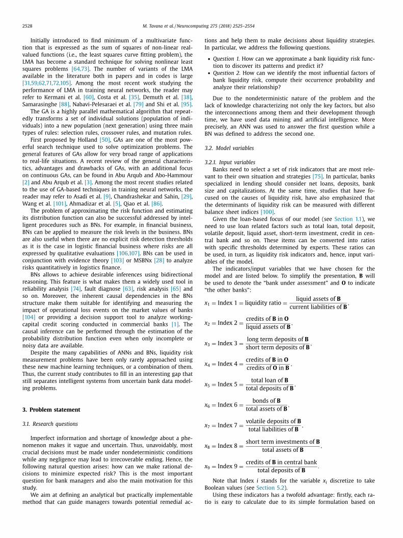
Fig. 1. Network architecture.
Table 1
Comparing several possible network architectures.
Network
structure
MSE (test
data)
Standard deviation
of residuals
Correlation
(target-output) epochs
9–1–1 5.5 e −3 4.3 e −3 0.97 121
9–3–1 7.7 e −4 7.7 e −4 0.98 37
9–5–1 3.4 e −6 1.0 e −5 0.98 143
9–7–1 4.1 e −9 5.6 e −6 1 356
9–8–1 3.6 e −8 3.7 e −5 1 875
9–1–1–1 2.5 e −8 3.3 e −5 0.99 837
9–2–1–1 9.7 e −8 1.0 e −5 0.99 10 0 0
9–2–2–1 8.2 e −8 3.1 e −5 1 10 0 0
9–2–3–1 1.1 e −7 2.4 e −6 1 10 0 0
9–3–2–1 7.2 e −7 7.1 e −6 1 10 0 0
9–4–2–1 5.6 e −8 5.1 e −6 1 10 0 0
9–4–3–1 2.7 e −11 7.1 e −6 1 10 0 0
m
s
e
L
t
b
b
t
h
f
i
d
(
5
w
l
c
b
w
m
w
u
d
p
(
m
w
t
t
t
t
A
s
(
w
t
T
t
m
where, N i jk is the number of samples in the k -th bin of the local
pdf of x i with the j-th parent configuration pa ( x i ) j .
Stage 3: Inference
Finally, the probability of any quantity Q( x 1 , x 2 , . . . , x 10 ) de-
pending on G and using the dataset Data can be calculated by av-
eraging over all possible values of the parameters weighted by the
posterior probability of each value. That is:
Pr ( Q( x 1 , x 2 , . . . , x 10 ) | G, Data )
=
∫ Q( x 1 , x 2 , . . . , x 10 ) Pr ( �| G, Data ) d�. (9)
For more convenience, the maximum likelihood (ML) of param-
eters is preferable rather than the entire distribution. The ML for
p i jk is:
ˆ p i jk =
N i jk + αi jk
N i j + αi j
. (10)
5. Case study: implementation of the proposed method
In this section, we show the results obtained by applying the
proposed liquidity risk measurement method to a set of real data
provided by a large U.S. bank focusing mainly on loans.
The collected dataset refers to a period of almost eight consecu-
tive years, from 2005 to 2011 plus a couple of months of 2004, and
were extracted from monthly reports. All ratios (i.e., our input and
output variables) were already normalized but had to be increased
in number via a standard averaging technique. The implemented
dataset consists of 353 rows of data with each row displaying the
values taken by the 10 variables in a month. More details about
the dataset are given in the Appendix, where some sample rows of
data are also provided.
5.1. Phase 1: implementation by ANN
We start by describing the structure of the ANN, learning al-
gorithms and network assessment procedures that were imple-
ented. After rearranging the outputs as an autoregressive time
eries, the ability of designed network to predict liquidity risk is
xamined.
All the codes and analyses of the section were written in MAT-
AB. For a better understanding of the practical implementation of
he model and its effectiveness, the codes for training the network
y LMA and by GA have been provided in the Appendix .
The input variables x 1 , . . . , x 9 and output variable x 10 have
een introduced in Section 3 together with the liquidity risk func-
ion, see Eq. (1) . In particular, the output x 10 , i.e., Current Ratio,
ad to account for a total of 353 data (see the Appendix ).
In this phase, the goal was to approximate the liquidity risk
unction, therefore we needed continuous data. Note that normal-
zation is the only necessary preprocessing of data. Also, data were
ivided into three groups: training (70%), validation (15%) and test
15%) data.
.1.1. Network architecture
The architecture chosen for the network is a three layer MLP
ith one hidden layer (corresponding to node 7) and one output
ayer (corresponding to node 1). The input layer contains 9 nodes
orresponding to the 9 inputs. The optimal structure was selected
y trial and error. The network architecture is shown is Fig. 1 .
The assessment (training, validation and testing) of the network
as performed using the well-known mean squared error (MSE)
ethod:
1
�
�∑
λ=1
( t λ − r λ) 2 , (11)
here: t λ is the λth component of the vector of observed real val-
es (target vector), r λ is the λth component of the vector of pre-
icted values (output vector), and � is the length of both the out-
ut and the target vectors.
In addition, the correlation between target values and outputs
R ), the mean ( μ), the variance of residuals ( σ 2 ), the second root of
ean squared error, and the learning process error (performance)
ere all used to assess the network.
Note that the network works properly with almost all the struc-
ures. Since in the majority of the cases one hidden layer is enough
o perform properly, we have considered several structures con-
aining one hidden layer and two hidden layers. Table 1 reports
he assessment results obtained by training the network by LMA.
s shown in Table 1 , among the analyzed structures, the 9–7–1
tructure is the simplest four layer structure and performs better
in terms of time and quality) than the other three layer structures.
Note also that due to the randomness at the basis of neural net-
orks, the quality of the approximation is highly dependent on
he samples selected for training. Thus, the numbers reported in
able 1 may change slightly within frequent running. At the same
ime, as the network structure becomes more complicated, it takes
ore time to be trained and the quality of results slowly decreases.

M. Tavana et al. / Neurocomputing 275 (2018) 2525–2554 2533
Fig. 2. Assessment of learning process on train data implemented by LMA.
5
f
t
p
m
n
t
i
w
(
r
d
w
b
t
n
a
m
r
5
t
d
i
a
fi
c
r
c
n
w
v
r
g
g
p
q
σ
r
F
i
a
d
o
r
a
v
l
t
t
s
t
v
a
L
.1.2. Training of ANN
The training process was conducted by LMA, which is the de-
ault training algorithm in MATLAB toolbox, and by GA. As men-
ioned earlier ( Section 2.1 ), LMA is an optimization algorithm very
opular for its applications in curve-fitting problems, but, like
any other optimization algorithms, it is affected by a main weak-
ess: it is able to find the local minimum which is not necessarily
he global minimum. Moreover, the quality of the answers is sat-
sfactory provided that the initial weights (hence, the initial net-
ork) is a relatively good guess and that the signal to noise ratio
SNR) is larger than five.
This is why we used in parallel a meta-heuristic search algo-
ithm, that is, GA. Since GA has a random behavior and does not
epend on the initial point, it was applied to make sure that LMA
as working correctly. Moreover, apart from avoiding some draw-
acks of LM (i.e., the risk of being trapped in a local minimum),
he implementation with GA emphasizes that the dataset is conve-
ient enough to be modeled with any other algorithm.
However, as it will be shown below, LMA performed consider-
bly better than GA and was able to recognize the pattern of data
uch more accurately. As a consequence, in the end, the liquidity
isk was modeled by LMA.
.1.3. Performance of LMA and GA in training ANN
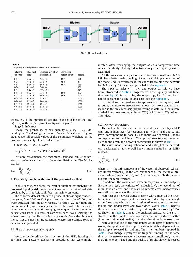
The charts in Figs. 2 –4 show the performance of LMA on the
hree separate groups of data including train, validation and test
ata.
The results obtained by assessing the network by GA are shown
n Figs. 5 and 6:
Figs. 2 –6 indicate the quality of learning by the algorithms GA
nd LMA. Each figure consists of four subfigures. The first sub-
gure, in the upper left quadrant, displays outputs and targets to
ompare how much the learned pattern (outputs) is similar to the
eal data (targets). The vertical axis shows the values 0 to 1 be-
ause all data were normalized. The horizontal axis refers to the
umber of samples for each group: to perform cross-validation,
e divided the dataset into three different groups of train data,
alidation data and test data. The second subfigure, in the upper
ight quadrant, depicts the correlation between outputs and tar-
ets. The third subfigure, in the lower left quadrant, provides a
raphical representation of the mean-squared error between out-
uts and targets. Finally, the fourth subfigure, in the lower right
uadrant, checks if the residuals have a normal distribution. In fact,
and MSE are the main measures indicating the quality of pattern
ecognition.
It is worth noting that the scales of the subfigures composing
igs. 2 –6 are all based on the accuracy of the network during train-
ng. In particular, training by GA leads to a weaker performance
nd larger standard deviation. This is the reason why there is a
ifference in scale between the figures (i.e., the small figures down
n the right) that account for training by LMA ( Figs. 2 –4 ) and those
eporting the results of training by GA.
Figs. 7 –9 complement the analysis of the performance of LMA
nd GA by showing the trends of the learning errors. Fig. 7 pro-
ides a graphical representation of the descending trend of the
earning error when training the network by GA. Fig. 8 compares
he trends of the learning errors relative to the train data, valida-
ion data and test data when training the network by LMA. Fig. 9
hows a comparison between the target values (i.e., the values of
he liquidity risk function based on real data) and the liquidity risk
alues learned by LMA.
Regarding the execution time of the algorithms, LMA allows for
reliable implementation in a relatively short time. The rapidity of
MA is one well-known advantage of this algorithm. On the other
2534 M. Tavana et al. / Neurocomputing 275 (2018) 2525–2554
Fig. 3. Assessment of learning process on validation data implemented by LMA.
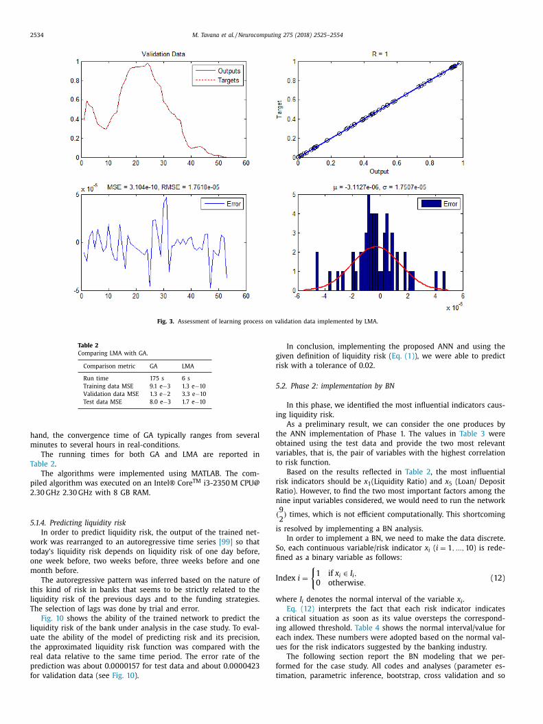
Table 2
Comparing LMA with GA.
Comparison metric GA LMA
Run time 175 s 6 s
Training data MSE 9.1 e −3 1.3 e −10
Validation data MSE 1.3 e −2 3.3 e −10
Test data MSE 8.0 e −3 1.7 e −10
g
r
5
i
t
o
v
t
r
R
n
i
S
fi
I
w
a
i
e
u
f
t
hand, the convergence time of GA typically ranges from several
minutes to several hours in real-conditions.
The running times for both GA and LMA are reported in
Table 2 .
The algorithms were implemented using MATLAB. The com-
piled algorithm was executed on an Intel® Core TM i3-2350 M CPU@
2.30 GHz 2.30 GHz with 8 GB RAM.
5.1.4. Predicting liquidity risk
In order to predict liquidity risk, the output of the trained net-
work was rearranged to an autoregressive time series [99] so that
today’s liquidity risk depends on liquidity risk of one day before,
one week before, two weeks before, three weeks before and one
month before.
The autoregressive pattern was inferred based on the nature of
this kind of risk in banks that seems to be strictly related to the
liquidity risk of the previous days and to the funding strategies.
The selection of lags was done by trial and error.
Fig. 10 shows the ability of the trained network to predict the
liquidity risk of the bank under analysis in the case study. To eval-
uate the ability of the model of predicting risk and its precision,
the approximated liquidity risk function was compared with the
real data relative to the same time period. The error rate of the
prediction was about 0.0 0 0 0157 for test data and about 0.0 0 0 0423
for validation data (see Fig. 10 ).
In conclusion, implementing the proposed ANN and using the
iven definition of liquidity risk ( Eq. (1) ), we were able to predict
isk with a tolerance of 0.02.
.2. Phase 2: implementation by BN
In this phase, we identified the most influential indicators caus-
ng liquidity risk.
As a preliminary result, we can consider the one produces by
he ANN implementation of Phase 1. The values in Table 3 were
btained using the test data and provide the two most relevant
ariables, that is, the pair of variables with the highest correlation
o risk function.
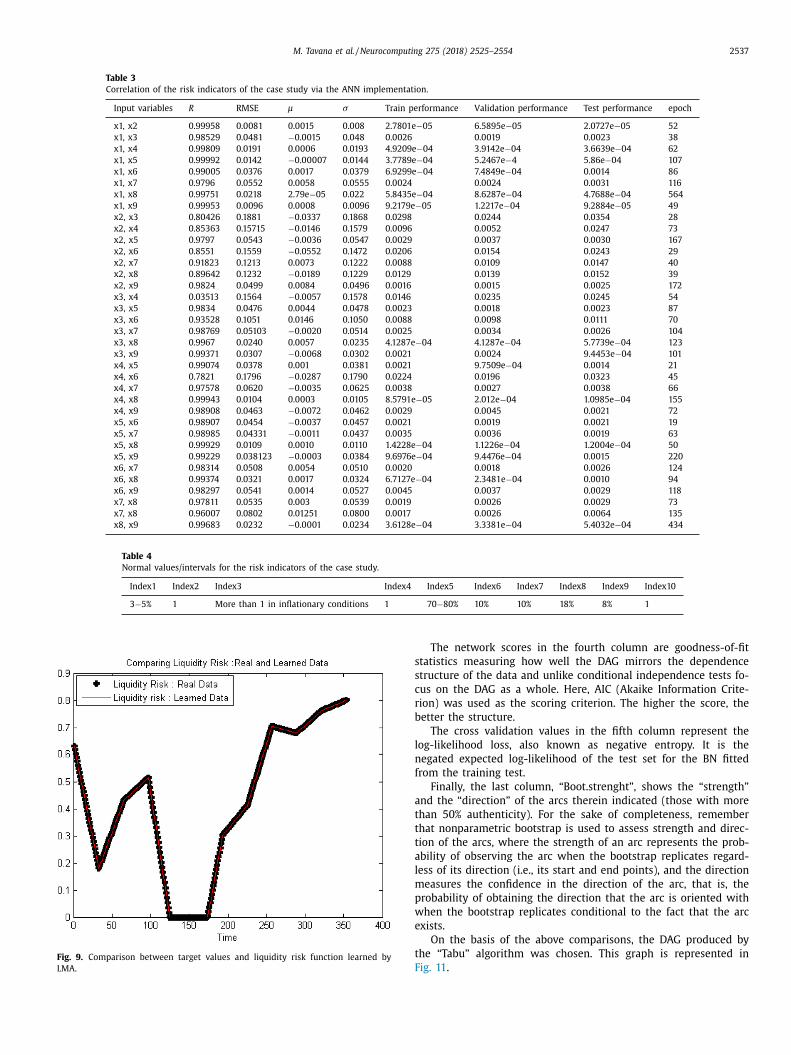
Based on the results reflected in Table 2 , the most influential
isk indicators should be x 1 (Liquidity Ratio) and x 5 (Loan/ Deposit
atio). However, to find the two most important factors among the
ine input variables considered, we would need to run the network
( 9
2 ) times, which is not efficient computationally. This shortcoming
s resolved by implementing a BN analysis.
In order to implement a BN, we need to make the data discrete.
o, each continuous variable/risk indicator x i ( i = 1 , ..., 10 ) is rede-
ned as a binary variable as follows:
ndex i =
{1 if x i ∈ I i , 0 otherwise .
(12)
here I i denotes the normal interval of the variable x i .
Eq. (12) interprets the fact that each risk indicator indicates
critical situation as soon as its value oversteps the correspond-
ng allowed threshold. Table 4 shows the normal interval/value for
ach index. These numbers were adopted based on the normal val-
es for the risk indicators suggested by the banking industry.
The following section report the BN modeling that we per-
ormed for the case study. All codes and analyses (parameter es-
imation, parametric inference, bootstrap, cross validation and so

M. Tavana et al. / Neurocomputing 275 (2018) 2525–2554 2535
Fig. 4. Assessment of learning process on test data implemented by LMA.
Fig. 5. Assessment of learning process of validation data implemented by GA.

2536 M. Tavana et al. / Neurocomputing 275 (2018) 2525–2554
Fig. 6. Assessment of learning process of test data implemented by GA.
Fig. 7. Descending trend of learning error by GA.
Fig. 8. Descending trends of learning errors by LMA.
w
t
i
s
o
(
S
c
g
o
on) were written in R using the packages “bnlearn”, “Rgraphviz”,
and “gRain”.
The computational complexity of the algorithms used in BNs
is polynomial in the number of tests, usually O ( N
2 ) (super-
exponential in the worst case scenario), where N is the number
of variables. Regarding the execution time, it scales linearly with
the size of the dataset.
5.2.1. Structure learning
To reduce the space of possible DAGs we used the eight algo-
rithms described in Stage 1 of Section 4.4.2 . Table 5 shows the fea-
tures of different implementations by these eight algorithms.
The acronyms of the algorithms appear in the first column
hile the second column shows the total number of conditional
ests used by the corresponding algorithm in the structure learn-
ng process. The third column titled “strength of arcs” shows the
trength of the probabilistic relationships expressed by the arcs
f a BN. When the criterion is a conditional independence test
constraint-based algorithms), the strength of an arc is a p -value.
o the lower the value, the stronger the relationship. When the
riterion is the label of a score function (score-based and hybrid al-
orithms), the strength of an arc is measured by a score (gain/loss)
n the basis of which the arc is kept or removed.
M. Tavana et al. / Neurocomputing 275 (2018) 2525–2554 2537
Table 3
Correlation of the risk indicators of the case study via the ANN implementation.
Input variables R RMSE μ σ Train performance Validation performance Test performance epoch
x1, x2 0.99958 0.0081 0.0015 0.008 2.7801e −05 6.5895e −05 2.0727e −05 52
x1, x3 0.98529 0.0481 −0.0015 0.048 0.0026 0.0019 0.0023 38
x1, x4 0.99809 0.0191 0.0 0 06 0.0193 4.9209e −04 3.9142e −04 3.6639e −04 62
x1, x5 0.99992 0.0142 −0.0 0 0 07 0.0144 3.7789e −04 5.2467e −4 5.86e −04 107
x1, x6 0.99005 0.0376 0.0017 0.0379 6.9299e −04 7.4 84 9e −04 0.0014 86
x1, x7 0.9796 0.0552 0.0058 0.0555 0.0024 0.0024 0.0031 116
x1, x8 0.99751 0.0218 2.79e −05 0.022 5.8435e −04 8.6287e −04 4.7688e −04 564
x1, x9 0.99953 0.0096 0.0 0 08 0.0096 9.2179e −05 1.2217e −04 9.2884e −05 49
x2, x3 0.80426 0.1881 −0.0337 0.1868 0.0298 0.0244 0.0354 28
x2, x4 0.85363 0.15715 −0.0146 0.1579 0.0096 0.0052 0.0247 73
x2, x5 0.9797 0.0543 −0.0036 0.0547 0.0029 0.0037 0.0030 167
x2, x6 0.8551 0.1559 −0.0552 0.1472 0.0206 0.0154 0.0243 29
x2, x7 0.91823 0.1213 0.0073 0.1222 0.0088 0.0109 0.0147 40
x2, x8 0.89642 0.1232 −0.0189 0.1229 0.0129 0.0139 0.0152 39
x2, x9 0.9824 0.0499 0.0084 0.0496 0.0016 0.0015 0.0025 172
x3, x4 0.03513 0.1564 −0.0057 0.1578 0.0146 0.0235 0.0245 54
x3, x5 0.9834 0.0476 0.0044 0.0478 0.0023 0.0018 0.0023 87
x3, x6 0.93528 0.1051 0.0146 0.1050 0.0088 0.0098 0.0111 70
x3, x7 0.98769 0.05103 −0.0020 0.0514 0.0025 0.0034 0.0026 104
x3, x8 0.9967 0.0240 0.0057 0.0235 4.1287e −04 4.1287e −04 5.7739e −04 123
x3, x9 0.99371 0.0307 −0.0068 0.0302 0.0021 0.0024 9.4453e −04 101
x4, x5 0.99074 0.0378 0.001 0.0381 0.0021 9.7509e −04 0.0014 21
x4, x6 0.7821 0.1796 −0.0287 0.1790 0.0224 0.0196 0.0323 45
x4, x7 0.97578 0.0620 −0.0035 0.0625 0.0038 0.0027 0.0038 66
x4, x8 0.99943 0.0104 0.0 0 03 0.0105 8.5791e −05 2.012e −04 1.0985e −04 155
x4, x9 0.98908 0.0463 −0.0072 0.0462 0.0029 0.0045 0.0021 72
x5, x6 0.98907 0.0454 −0.0037 0.0457 0.0021 0.0019 0.0021 19
x5, x7 0.98985 0.04331 −0.0011 0.0437 0.0035 0.0036 0.0019 63
x5, x8 0.99929 0.0109 0.0010 0.0110 1.4228e −04 1.1226e −04 1.2004e −04 50
x5, x9 0.99229 0.038123 −0.0 0 03 0.0384 9.6976e −04 9.4476e −04 0.0015 220
x6, x7 0.98314 0.0508 0.0054 0.0510 0.0020 0.0018 0.0026 124
x6, x8 0.99374 0.0321 0.0017 0.0324 6.7127e −04 2.3481e −04 0.0010 94
x6, x9 0.98297 0.0541 0.0014 0.0527 0.0045 0.0037 0.0029 118
x7, x8 0.97811 0.0535 0.003 0.0539 0.0019 0.0026 0.0029 73
x7, x8 0.96007 0.0802 0.01251 0.0800 0.0017 0.0026 0.0064 135
x8, x9 0.99683 0.0232 −0.0 0 01 0.0234 3.6128e −04 3.3381e −04 5.4032e −04 434
Table 4
Normal values/intervals for the risk indicators of the case study.
Index1 Index2 Index3 Index4 Index5 Index6 Index7 Index8 Index9 Index10
3 −5% 1 More than 1 in inflationary conditions 1 70 −80% 10% 10% 18% 8% 1
Fig. 9. Comparison between target values and liquidity risk function learned by
LMA.
s
s
c
r
b
l
n
f
a
t
t
t
a
l
m
p
w
e
t
F
The network scores in the fourth column are goodness-of-fit
tatistics measuring how well the DAG mirrors the dependence
tructure of the data and unlike conditional independence tests fo-
us on the DAG as a whole. Here, AIC (Akaike Information Crite-
ion) was used as the scoring criterion. The higher the score, the
etter the structure.
The cross validation values in the fifth column represent the
og-likelihood loss, also known as negative entropy. It is the
egated expected log-likelihood of the test set for the BN fitted
rom the training test.
Finally, the last column, “Boot.strenght”, shows the “strength”
nd the “direction” of the arcs therein indicated (those with more
han 50% authenticity). For the sake of completeness, remember
hat nonparametric bootstrap is used to assess strength and direc-
ion of the arcs, where the strength of an arc represents the prob-
bility of observing the arc when the bootstrap replicates regard-
ess of its direction (i.e., its start and end points), and the direction
easures the confidence in the direction of the arc, that is, the
robability of obtaining the direction that the arc is oriented with
hen the bootstrap replicates conditional to the fact that the arc
xists.
On the basis of the above comparisons, the DAG produced by
he “Tabu” algorithm was chosen. This graph is represented in
ig. 11 .

2538 M. Tavana et al. / Neurocomputing 275 (2018) 2525–2554
Table 5
The structure learning algorithms used in the case study for the BN approach.
Structure learning algorithms Number of tests Strength of arcs Scores Cross validation Boot.strength
gs 180 x1 to x2 8.500840e −11
x1 to x4 2.796285e −34
x3 to x1 4.481730e −02 x2 to x5 0.540 0.5578125
x3 to x5 3.840679e −04 x2 to x10 1.0 0 0 0.94750 0 0
x5 to x2 1.203200e −05 −1178.755 3.271185 x4 to x1 0.500 0.5225000
x5 to x4 3.567837e −08 x5 to x4 0.185 0.8659898
x6 to x4 3.216251e −07 x10 to x1 0.515 0.5582524
x9 to x8 1.545431e −15
x10 to x1 3.545118e −02
x10 to x2 3.343556e −13
iamb 230 x4 to x4 5.405356e −11
x2 to x10 6.225173e −13 x3 to x5 0.565 0.6548673
x3 to x5 3.840679e −04 x4 to x1 0.500 0.7600000
x4 to x1 1.298065e −46 x4 to x2 1.0 0 0 0.8255474
x4 to x9 3.287519e −06 −1110.694 3.104175 x4 to x5 0.980 0.6454082
x5 to x4 5.243456e −08 x7 to x6 0.525 0.5476190
x7 to x6 1.466314e −06 x9 to x8 0.535 0.5427807
x8 to x7 3.079938e −13 x10 to x1 0.515 0.9024390
x9 to x8 1.545431e −15 x10 to x2 0.500 0.5225000
x10 to x1 2.881926e −11
fast.iamb 181 x1 to x3 8.377670e −03
x2 to x4 5.405356e −11
x2 to x10 6.225173e −13 x2 to x10 1.0 0 0 0.910 0 0 0 0
x4 to x1 1.298065e −46 x3 to x5 0.535 0.6401869
x5 to x3 2.707942e −04 −1161.68 3.186626 x4 to x1 0.510 0.70250 0 0
x5 to x4 5.243456e −08 x4 to x5 0.990 0.8616162
x7 to x9 9.824817e −01 x8 to x9 1.0 0 0 0.6929825
x8 to x9 2.030499e −05 x10 to x1 0.590 0.7584746
x10 to x1 2.881926e −11
x10 to x3 2.711597e −03
inter.iamb 236 x2 to x4 5.405356e −11
x2 to x10 6.225173e −13
x3 to x5 3.840679e −04 x2 to x5 0.505 0.6188119
x4 to x1 1.298065e −46 x2 to x10 1.0 0 0 0.820 0 0 0 0
x4 to x9 3.287519e −06 x4 to x1 0.512 0.5850 0 0 0
x5 to x4 5.243456e −08 −1108.448 3.131317 x4 to x5 0.990 0.6237374
x7 to x6 1.466314e −06 x5 to x3 1.0 0 0 0.7141509
x8 to x7 3.079938e −13 x8 to x9 0.815 0.6625767
x9 to x8 1.545431e −15 x10 to x1 0.505 0.7079208
x10 to x1 2.881926e −11
x10 to x3 1.291410e −03
hc 162 x1 to x4 −91.365802
x4 to x2 −29.307835 x1 to x4 1.0 0 0 0.88250 0 0
x8 to x9 −28.854619 x1 to x10 0.975 0.9222222
x7 to x8 −23.646469 x2 to x10 1.0 0 0 0.68250 0 0
x2 to x10 −19.298749 x4 to x2 0.925 0.9135135
x4 to x5 −24.156349 x4 to x5 0.975 0.9743590
x9 to x4 −18.264567 −1086.245 2.933348 x5 to x3 0.810 0.8950617
x6 to x7 −8.664017 x7 to x6 0.5140.5888889
x8 to x5 −5.098120 x8 to x7 0.6170.580 0 0 0 0
x1 to x10 −19.300574 x9 to x4 0.925 0.9324324
x4 to x10 −9.738446 x9 to x8 0.975 0.5769231
x5 to x3 −3.372261 x10 to x4 0.840 0.5833333
x9 to x1 −2.329284
tabu 342 x1 to x4 −91.365802 −1086.245 2.881097 x1 to x4 1.0 0 0 0.7950 0 0 0
x4 to x2 −29.307835 x1 to x10 0.790 0.8132911
x8 to x9 −28.854619 x2 to x10 1.0 0 0 0.76250 0 0
x7 to x8 −23.646469 x4 to x2 0.920 0.8929348
x2 to x10 −19.298749 x4 to x5 0.975 0.9153846
x4 to x5 −24.156349 x5 to x3 0.840 0.7946429
x9 to x4 −18.264567 x7to x6 0.880 0.7272727
x6 to x7 −8.664017 x8 to x5 0.585 0.7521368
x8 to x5 −5.098120 x8 to x7 0.990 0.8262626
x1 to x10 −19.300574 x9 to x4 0.935 0.6016043
x4 to x10 −9.738446 x9 to x8 0.935 0.7497326
x5 to x3 −3.372261 x10 to x4 0.835 0.6209581
x9 to x1 −2.329284
mmhc 200 x1 to x4 −84.513668
x8 to x9 −28.854619 x1 to x4 1.0 0 0 0.730 0 0 0 0
x2 to x10 −27.136282 x2 to x10 1.0 0 0 0.7050 0 0 0
x4 to x5 −22.430489 −1155.408 3.175855 x4 to x2 0.875 0.7259259
x1 to x2 −13.625433 x4 to x5 0.985 0.8197970
x5 to x2 −8.944814 x5 to x3 0.820 0.5396341
x6 to x4 −5.555694 x9 to x4 0.935 0.8622047
( continued on next page )

M. Tavana et al. / Neurocomputing 275 (2018) 2525–2554 2539
Table 5 ( continued )
Structure learning algorithms Number of tests Strength of arcs Scores Cross validation Boot.strength
x1 to x10 −3.782643 x9 to x8 0.4310.502777
x5 to x3 −3.372261
rsmax2 142 x1 to x4 −91.365802
x4 to x2 −29.307835 x1 to x4 1.0 0 0 0.80750 0 0
x8 to x9 −28.854619 x1 to x10 1.0 0 0 0.9807692
x2 to x10 −22.955488 −1130.84 3.290227 x2 to x10 1.0 0 0 0.94250 0 0
x4 to x5 −22.430489 x4 to x5 1.0 0 0 0.8550 0 0 0
x9 to x4 −18.264567 x5 to x2 0.535 0.9439252
x6 to x7 −8.664017 x5 to x3 0.805 0.6386139
x5 to x3 −3.372261
Fig. 10. Precision of prediction in ANN.
X6
X7
X8X5 X9
X1X4X3
X10X2
Fig. 11. Learned Bayesian Network to determine the most influential risk indicators.
D
t
e
H
t
P
t
B
w
r
p
t
I
t
d
5
w
a
w
n
t
H
b
t
v
−
w
m
o
o
5
q
v
o
v
i
w
d
i
t
To assess whether the probabilistic dependence of the selected
AG is supported by the data, we also run another structure test,
he Conditional Independence Test.
Given a causal chain of three nodes, A , B and C, the null hypoth-
sis is:
0 = A ⊥⊥ C| B
hat is, “A is conditionally independent from C given B ”(i.e.,
r (C| A ∧ B ) = Pr (C| B ) ). The alternative hypothesis is:
hat is, “A is conditionally dependent from C given B ” (i.e., Pr (C| A ∧ ) = Pr (C| B ) ).
Here, the independence criterion is Mutual Information (mi)
ith α = 0 . 05 (first type error). Therefore, the null hypothesis is
ejected if p −value < α. If the null hypothesis (conditional inde-
endence) is rejected, the arc can be considered for inclusion in
he DAG.
Table 6 shows the results obtained by running the Conditional
ndependence Test on all the arcs of the graph in Fig. 11 in order
o investigate the authenticity of the arcs. The test confirmed the
ependences among the arcs obtained by Tabu.
.2.2. Parameter learning
The parameter learning process is performed by a function
hich fits the parameters of the selected BN given its structure
nd the available dataset. As described in Stage 2 of Section 4.4.2 ,
e used the Maximum Likelihood parameter estimation.
Table 7 represents the conditional probability tables of all the
odes endowed with multinomial distributions. “True” means that
he corresponding index is in its normal interval.
At the point, the network was built and the parameters fitted.
ence, the risk function which was built earlier by ANN, was now
uilt by BN and the results compared.
Before moving on to the inference stage, two assessment cri-
eria were used to score the fitted BN for which a log-likelihood
alue can be obtained, according to following formula:
2 × log −l ikel ihood + k × npar, (13)
here npar represents the number of parameters in the fitted
odel, k = 2 for the usual AIC, and k = log (n ) , with n number
f observations, for BIC or SBC (Schwarz’s Bayesian criterion). We
btained:
Akaike Information Criterion = −1030.223
Bayesian Information Criterion = −1086.245
(The higher value is better.)
.2.3. Inference
After the parameter estimation, we were able to answer the
uestion of what are the influential factors for liquidity risk by pro-
iding a classification of them from the most to the less influential
ne. We followed the procedure below.
Suppose that all of the liquidity risk indicators show normal
alues except for Index 1; hence, measure the marginal probabil-
ty of liquidity risk by these evidences. Repeat the same operation
ith a little change in the evidences, that is, assuming that all in-
icators show normal values apart from Index 2. Repeat for each
ndicator until the last one. Table 8 shows the marginal probabili-
ies obtained through this process.

2540 M. Tavana et al. / Neurocomputing 275 (2018) 2525–2554
Table 6
Conditional independence test on the Bayesian Network
learned in the case study ( Fig. 7 ).
Arcs ci.test
x9 → x1 data: x9–x1
mi = 10.522, df = 1, p -value = 0.001179
x1 → x4 data: x1–x4
mi = 167.84, df = 1, p -value < 2.2e −16
x4 → x2 data: x4–x2
mi = 64.479, df = 1, p -value = 9.755e −16
x8 → x9 data: x8–x9
mi = 63.573, df = 1, p -value = 1.545e −15
x7 → x8 data: x7–x8
mi = 53.157, df = 1, p -value = 3.08e −13
x2 → x10 data: x2–x10
mi = 51.775, df = 1, p -value = 6.225e −13
x4 → x5 data: x4–x5
mi = 50.725, df = 1, p -value = 1.063e −12
x9 → x4 data: x9–x4
mi = 21.641, df = 1, p -value = 3.288e −06
x6 → .x7 data: x6–x7
mi = 23.192, df = 1, p -value = 1.466e −06
x8 → x5 data: x8–x5
mi = 12.608, df = 1, p -value = 0.0 0 03841
x1 → x10 data: x1–x10
mi = 5.0673, df = 1, p -value = 0.02438
x4 → x10 data: x4–x10
mi = 3.4066, df = 1, p -value = 0.06494
x5 → x3 data: x5–x3
mi = 12.608, df = 1, p -value = 0.0 0 03841
x1, x9 | x4 data: x1–x9 | x4
mi = 37.138, df = 2, p -value = 8.623e −09
x4, x8 | x5 data: x4–x8 | x5
mi = 22.133, df = 2, p -value = 1.562e −05
x1, x2 | x10 data: x1–x4 | x10
mi = 211.32, df = 2, p -value < 2.2e −16
x1, x4| x10 data: x2–x4 | x10
mi = 61.241, df = 2, p -value = 5.031e −14
x2, x4 | x10 data: x2–x4 | x10
mi = 61.241, df = 2, p -value = 5.031e −14
p
m
n
v
p
k
a
i
w
t
t
p
f
r
s
p
F
d
b
6
a
b
c
n
e
t
v
l
c
t
A
T
s
b
m
t
T
s
i
l
t
d
s
m
l
g
a
t
a
s
o
p
From the values reported in Table 8 , it follows that x 1 and x 5 are the most influential factors, confirming the results shown by
Table 3 .
Note that once the parameter have been estimated, we can
actually answer any question about liquidity risk and its factors
by joint, conditional and marginal probability functions. Package
“gRain” provides some functions in order to have exact inferences.
For example, we could be interested in knowing the probability
that liquidity risk occurs (a) given that all the risk indicators (vari-
ables) have been measured or (b) when not all the indicators have
been measured.
Point (a) can be addressed considering the marginal probability
of the liquidity risk function with the evidence including all nine
indicators and it returns almost 69%, which actually reflects the
current total liquidity risk of bank used in the case study. Regard-
ing point (b), it is possible to measure liquidity risk even if only
some indicators are measured. Suppose, for instance, that x 2 , x 3 ,
x 4 and x 8 are the only indicators that have been measured, and
that x 3 and x 4 take their normal values while x 2 and x 8 do not.
Then, the marginal probability of variable x 10 (liquidity risk) would
return the values 0.650425 and 0.349575 for liquidity risk not oc-
curring and occurring, respectively. That is, we would face 35% liq-
uidity risk under the given conditions.
5.3. Remarks on testing and validation
Given that the machine learning approaches used in this paper
are based on learning via data, the validation processes are to be
defined within the methods being applied. More precise, when ap-
roximating a function by ANN, measures like bias, variance and
ean-squared error are employed to indicate how correctly the
etwork is learning. A similar reasoning is true for BN where the
alidity of the scores obtained at each stage of the structure and
arameter learning phases is confirmed by several tests, such as
-fold cross-validation, independence test, and bootstrap.
In other words, the best and, probably, the only way to validate
machine learning model is to analyze the quality of its learn-
ng: all the tools required for such an analysis are already available
ithin the single techniques employed by the model itself.
To better illustrate this fact, we provide a simulation showing
he quality of parameter learning in the proposed BN. Using the
rained network, we have generated 30 samples from the learned
df for each one of the 10 available variables. The pdfs resulting
rom the simulation are represented in Fig. 12 .
The variables can take only two values, TRUE or FALSE, that cor-
espond to the numbers 0 and 1 along the vertical axis. Fig. 12. a
hows the real data while Fig. 12. b provides a graphic of the sam-
le pdf generated by the trained network. As it can be observed in
ig. 12 , the network was able to estimate the pdf properly. The in-
ents appearing in Fig. 12. b are to be interpreted as mistakes made
y the network while performing the estimation.
. Conclusion
This study has addressed the problem of defining an efficient
nd systematic method to prudently handle and correctly evaluate
ank liquidity risk.
The ambiguity and vagueness that characterize the liquidity risk
oncept make difficult the formulation of an unquestionable defi-
ition for it. Identifying the factors that determine and/or influ-
nce liquidity risk and formulating an appropriate functional form
o approximate and predict its value represent an even more in-
olved task. At the same time, the complexity and spread of the
iquidity risk phenomenon make obsolete the classical mathemati-
al modeling approaches.
To deal with these issues, we have proposed a method that uses
wo among the most recent machine learning techniques, namely,
rtificial Neural Networks (ANNs) and Bayesian Networks (BNs).
he variables of the model are liquidity ratios and have been cho-
en on the basis of the data usually available from a standard bank
alance sheet.
Despite the many capabilities of ANNs and BNs, liquidity risk
easurement problems have been only rarely approached using
hese new machine learning techniques, or a combination of them.
hus, the current study contributes to fill in an interesting gap that
till separates intelligent systems from uncertain bank data model-
ng problems.
We have focused on the concept of solvency as definition of the
iquidity risk. As a consequence, we have used endogenous factors
o construct a model whose characteristics allow to specifically ad-
ress loan-based liquidity risk prediction issues.
A case study based on real bank data has been presented to
how the efficiency, accuracy, rapidity and flexibility of data mining
ethods when modeling ambiguous occurrences related to bank
iquidity risk measurement.
The ANN and the BN implementations were capable of distin-
uishing the most critical risk factors and measuring the risk by
functional approximation and a distributional estimation, respec-
ively. Both models were assessed through their specific training
nd learning processes and returned very consistent results.
Moreover, the numerical results obtained in the case study
howed the ability of the proposed two-phase ANN-BN approach
f somehow “self-confirming” the results via an independent and
arallel implementation of the same dataset.

M. Tavana et al. / Neurocomputing 275 (2018) 2525–2554 2541
Table 7
Conditional probability tables of all the variables.
Table 8
Effect of each risk indicator on liquidity risk.
The effect of first indicator on liquidity risk while other indicators show normal situation 0.7038534
The effect of second indicator on liquidity risk while other indicators show normal situation 0.4971152
The effect of third indicator on liquidity risk while other indicators show normal situation 0.4377303
The effect of forth indicator on liquidity risk while other indicators show normal situation 0.3948898
The effect of fifth indicator on liquidity risk while other indicators show normal situation 0.6810290
The effect of sixth indicator on liquidity risk while other indicators show normal situation 0.4418040
The effect of seventh indicator on liquidity risk while other indicators show normal situation 0.4459734
The effect of eighth indicator on liquidity risk while other indicators show normal situation 0.0346395
The effect of ninth indicator on liquidity risk while other indicators show normal situation 0.4557452
a
b
i
i
r
fi
d
m
Considering the fact that the variables of the proposed model
re liquidity ratios easily computable using the data available in
alance sheets and that these also are the only data necessary to
mplement the model, with no need for complicated preprocess-
ng of data, managers can use the proposed model to infer about
isk factors and liquidity risk occurrences without any relevant dif-
culty or restriction.
It must be noted that the loan-based constraint imposed by the
efinition adopted for liquidity risk represents a limitation of the
odel. However, this limitation should be compensated by the fact
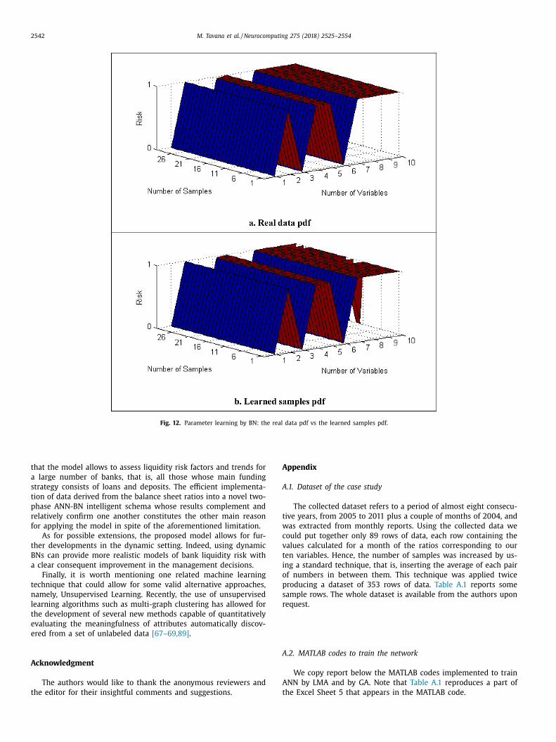
2542 M. Tavana et al. / Neurocomputing 275 (2018) 2525–2554
Fig. 12. Parameter learning by BN: the real data pdf vs the learned samples pdf.
A
A
t
w
c
v
t
i
o
p
s
r
A
A
t
that the model allows to assess liquidity risk factors and trends for
a large number of banks, that is, all those whose main funding
strategy consists of loans and deposits. The efficient implementa-
tion of data derived from the balance sheet ratios into a novel two-
phase ANN-BN intelligent schema whose results complement and
relatively confirm one another constitutes the other main reason
for applying the model in spite of the aforementioned limitation.
As for possible extensions, the proposed model allows for fur-
ther developments in the dynamic setting. Indeed, using dynamic
BNs can provide more realistic models of bank liquidity risk with
a clear consequent improvement in the management decisions.
Finally, it is worth mentioning one related machine learning
technique that could allow for some valid alternative approaches,
namely, Unsupervised Learning. Recently, the use of unsupervised
learning algorithms such as multi-graph clustering has allowed for
the development of several new methods capable of quantitatively
evaluating the meaningfulness of attributes automatically discov-
ered from a set of unlabeled data [67–69,89] .
Acknowledgment
The authors would like to thank the anonymous reviewers and
the editor for their insightful comments and suggestions.
ppendix
.1. Dataset of the case study
The collected dataset refers to a period of almost eight consecu-
ive years, from 2005 to 2011 plus a couple of months of 2004, and
as extracted from monthly reports. Using the collected data we
ould put together only 89 rows of data, each row containing the
alues calculated for a month of the ratios corresponding to our
en variables. Hence, the number of samples was increased by us-
ng a standard technique, that is, inserting the average of each pair
f numbers in between them. This technique was applied twice
roducing a dataset of 353 rows of data. Table A.1 reports some
ample rows. The whole dataset is available from the authors upon
equest.
.2. MATLAB codes to train the network
We copy report below the MATLAB codes implemented to train
NN by LMA and by GA. Note that Table A.1 reproduces a part of
he Excel Sheet 5 that appears in the MATLAB code.

M. Tavana et al. / Neurocomputing 275 (2018) 2525–2554 2543
Table A.1
Dataset of the case study.
Row of data Variable x 1 Variable x 2 Variable x 3 Variable x 4 Variable x 5 Variable x 6 Variable x 7 Variable x 8 Variable x 9 Variable x 10
Index 1 Index 2 Index 3 Index 4 Index 5 Index 6 Index 7 Index 8 Index 9 Index 10
1 0,193,816 0,09,1524 0 0,154,562 0,613,214 0 3,31E −05 0,0,9434 0,900,036 0,169,412
2 0,209,801 0,09,1215 0,0,08,427 0,167,297 0,618,891 0,00,368 3,26E −05 0,09,6622 0,899,047 0,183,493
3 0,225,786 0,09,0906 0,01,6854 0,180,032 0,624,568 0,00,736 3,21E −05 0,09,8904 0,898,058 0,197,573
4 0,241,771 0,09,0597 0,02,5281 0,192,766 0,630,245 0,0,1104 3,16E −05 0,101,186 0,89,707 0,211,654
5 0,257,757 0,09,0288 0,03,3708 0,205,501 0,635,922 0,0,1472 3,11E −05 0,103,468 0,896,081 0,225,735
6 0,273,742 0,08,9979 0,04,2136 0,218,236 0,641,599 0,0184 3,06E −05 0,10,575 0,895,093 0,239,815
7 0,289,727 0,0,8967 0,05,0563 0,23,097 0,647,276 0,0,2208 3,01E −05 0,108,032 0,894,104 0,253,896
8 0,305,712 0,08,9361 0,0,5899 0,243,705 0,652,953 0,0,2576 2,96E −05 0,110,315 0,893,116 0,267,976
9 0,321,698 0,08,9052 0,06,7417 0,25,644 0,65,863 0,0,2944 2,91E −05 0,112,597 0,892,127 0,282,057
10 0,337,683 0,08,8744 0,07,5844 0,269,174 0,664,307 0,0,3312 2,86E −05 0,114,879 0,891,138 0,296,137
… … … … … … … … … … …
101 0,399,562 0,0,8634 0,269,146 0,112,354 0,792,233 0,147,474 0,01,3007 0,864,888 0,880,486 0,35,914
102 0,416,383 0,08,7278 0,272,937 0,140,443 0,799,653 0,148,525 0,01,6259 0,869,713 0,880,149 0,377,639
103 0,433,204 0,08,8216 0,276,729 0,168,531 0,807,073 0,149,576 0,01,9511 0,874,538 0,879,812 0,396,139
104 0,450,025 0,08,9154 0,28,052 0,19,662 0,814,493 0,150,627 0,02,2762 0,879,364 0,879,475 0,414,639
105 0,466,846 0,09,0091 0,284,311 0,224,708 0,821,914 0,151,678 0,02,6014 0,884,189 0,879,138 0,433,138
106 0,483,666 0,09,1029 0,288,102 0,252,797 0,829,334 0,152,729 0,02,9266 0,889,015 0,8788 0,451,638
107 0,500,487 0,09,1967 0,291,894 0,280,885 0,836,754 0,15,378 0,03,2518 0,89,384 0,878,463 0,470,138
108 0,517,308 0,09,2905 0,295,685 0,308,974 0,844,174 0,154,831 0,0,3577 0,898,666 0,878,126 0,488,638
109 0,534,129 0,09,3843 0,299,476 0,337,062 0,851,595 0,155,882 0,03,9021 0,903,491 0,877,789 0,507,137
110 0,55,095 0,0,9478 0,303,268 0,365,151 0,859,015 0,156,934 0,04,2273 0,908,317 0,877,452 0,525,637
… … … … … … … … … … …
200 0,268,221 0,384,881 0,5815 0,914,702 0,781,558 0,264,733 0,120,939 0,413,635 0,680,818 0,474,764
201 0,258,043 0,409,486 0,562,341 0,902,516 0,777,159 0,294,144 0,12,619 0,399,565 0,683,055 0,471,321
202 0,247,865 0,434,091 0,543,183 0,890,331 0,772,761 0,323,555 0,131,442 0,385,495 0,685,293 0,467,879
203 0,237,687 0,458,695 0,524,024 0,878,145 0,768,363 0,352,965 0,136,693 0,371,425 0,68,753 0,464,436
204 0,22,751 0,4833 0,504,865 0,86,596 0,763,964 0,382,376 0,141,944 0,357,355 0,6 89,76 8 0,460,994
205 0,217,332 0,507,905 0,485,707 0,853,774 0,759,566 0,411,787 0,147,196 0,343,285 0,692,005 0,457,552
… … … … … … … … … … …
300 0,215,287 0,01,0654 0,77,338 0,208,825 0,38,271 0,10,226 0,5203 0,04,3809 0,27,194 0,09,2321
301 0,209,893 0,01,1622 0,752,778 0,212,368 0,372,153 0,100,897 0,543,143 0,04,2392 0,26,852 0,08,9754
302 0,204,499 0,01,2591 0,732,176 0,21,591 0,361,596 0,09,9534 0,565,985 0,04,0976 0,265,099 0,08,7188
303 0,199,105 0,0,1356 0,711,574 0,219,452 0,351,039 0,09,8172 0,588,828 0,0,3956 0,261,678 0,08,4621
304 0,193,711 0,01,4528 0,690,972 0,222,994 0,340,482 0,09,6809 0,611,671 0,03,8143 0,258,258 0,08,2055
305 0,188,317 0,01,5497 0,670,371 0,226,536 0,329,925 0,09,5446 0,634,514 0,03,6727 0,254,837 0,07,9488
… … … … … … … … … … …
349 0,01,2752 0,112,183 0,527,678 0,354,158 0,02,0126 0,139,217 0,748,121 0,0,01,758 0,02,5014 0,0,04,803
350 0,0,09,564 0,115,082 0,534,354 0,356,692 0,01,5095 0,141,559 0,739,125 0,0,01,319 0,0,1876 0,0,03,602
351 0,0,06,376 0,117,982 0,541,031 0,359,226 0,01,0063 0,143,901 0,730,129 0,0 0 0,879 0,01,2507 0,0,02,401
352 0,0,03,188 0,120,881 0,547,707 0,36,176 0,0,05,032 0,146,243 0,721,134 0,00,044 0,0,06,253 0,0,01,201
353 0 0,123,781 0,554,383 0,364,294 0 0,148,585 0,712,138 0 0 0
A
.2.1. MATLAB code for the training of ANN by LMA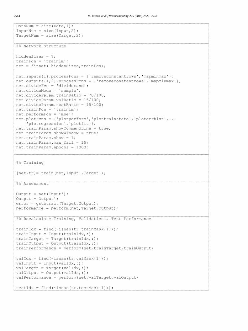
2544 M. Tavana et al. / Neurocomputing 275 (2018) 2525–2554

M. Tavana et al. / Neurocomputing 275 (2018) 2525–2554 2545

2546 M. Tavana et al. / Neurocomputing 275 (2018) 2525–2554
A.2.2. MATLAB code for the training of ANN by GA:

M. Tavana et al. / Neurocomputing 275 (2018) 2525–2554 2547

2548 M. Tavana et al. / Neurocomputing 275 (2018) 2525–2554

M. Tavana et al. / Neurocomputing 275 (2018) 2525–2554 2549
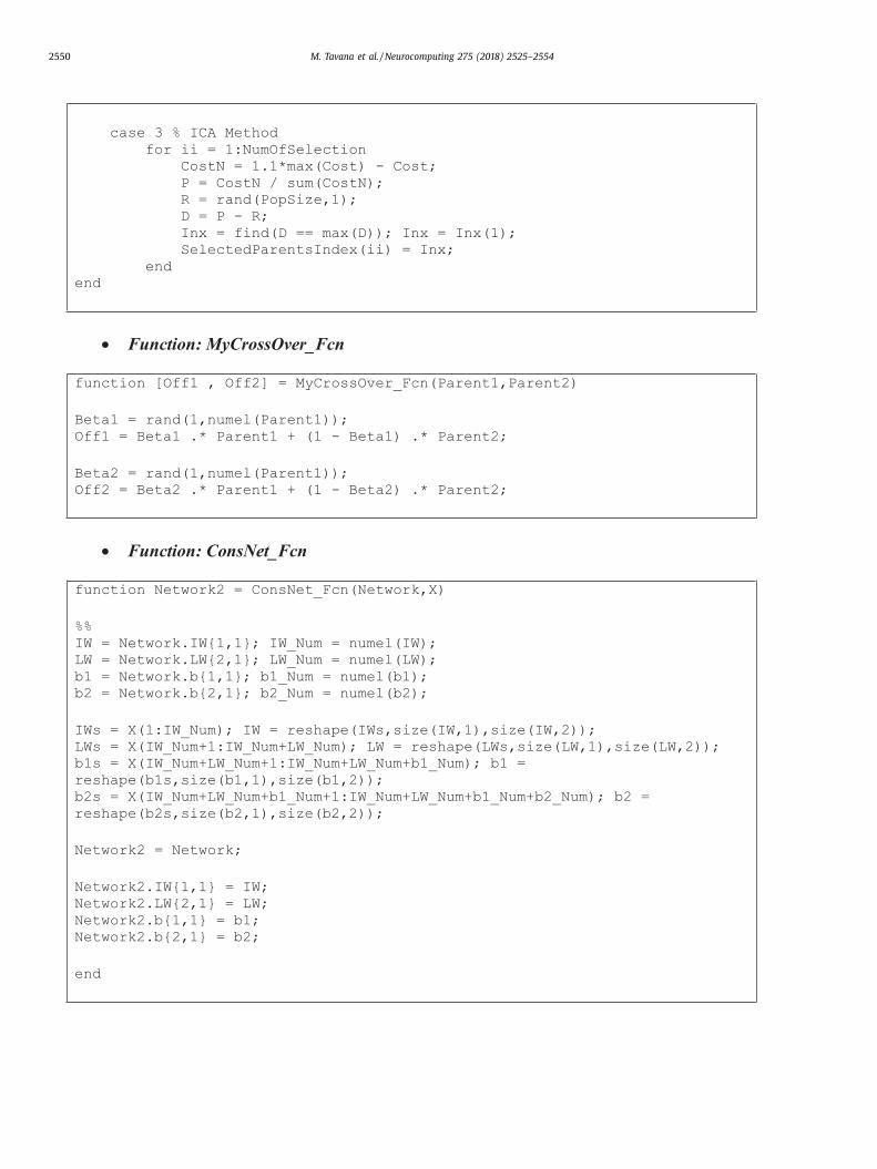
2550 M. Tavana et al. / Neurocomputing 275 (2018) 2525–2554
M. Tavana et al. / Neurocomputing 275 (2018) 2525–2554 2551

2552 M. Tavana et al. / Neurocomputing 275 (2018) 2525–2554
References
[1] W. Abramowicz , M. Nowak , J. Sztykiel , Bayesian networks as a decision
support tool in credit scoring domain, in: P.C. Pendharkar (Ed.), Managing
Data Mining Technologies in Organizations, IGI Publishing, Hershey, 2003,pp. 1–20 .
[2] O. Abu Arqub , Z. Abo-Hammour , Numerical solution of systems of sec-ond-order boundary value problems using continuous genetic algorithm, Inf.
Sci. 279 (2014) 396–415 . [3] O. Abu Arqub , Z.S. Abo-Hammour , S. Momani , Application of continuous ge-
netic algorithm for nonlinear system of second-order boundary value Prob-
lems, Appl. Math. Inf. Sci. 8 (1) (2014) 235–248 . [4] N. Ahmed , Z. Ahmed , I.H. Naqvi , Liquidity risk and islamic banks: evidence
from Pakistan, Interdiscip. J. Res. Bus. 1 (9) (2011) 99–102 . [5] F. Ahmadizar , K. Soltanian , F. AkhlaghianTab , I. Tsoulos , Artificial neural net-
work development by means of a novel combination of grammatical evolu-tion and genetic algorithm, Eng. Appl. Artif. Intell. 39 (2015) 1–13 .
[6] F. Allen , A. Babus , E. Carletti , Asset commonality, debt maturity and systemicrisk, J. Financ. Econ. 104 (2012) 519–534 .
[7] A. Angora , C. Roulet , Transformation Risk and its Determinants: A New Ap-
proach Based on Basel III Liquidity Management Framework, SSRN, 2011 . [8] A . Arif , N.A . Anees , Liquidity risk and performance in the banking system, J.
Financ. Regul. Compliance 20 (2) (2012) 182–195 . [9] E. Asadi , M.G. da Silva , C.H. Antunes , L. Dias , L. Glicksman , Multi-objective
optimization for building retrofit: a model using genetic algorithm and ar-tificial neural network and an application, Energy Build. 81 (2014) 4 4 4–
456 .
[10] P.P. Athanasoglou , S.N. Brissmis , M.D. Delis , Bank-specific, industry-specificand macroeconomic determinants of bank profitability, J. Int. Financ. Mark.
Inst. Money 18 (2008) 121–136 . [11] A.F. Atiya , Bankruptcy prediction for credit risk using neural networks:
a survey and new results, IEEE Trans. Neural Netw. 12 (4) (2001) 929–935 .
[12] J.R. Barth , D.E. Nolle , T. Phumiwasana , G. Yago , A cross-country analysis of
the bank supervisory framework and bank performance, Financ. Mark. Inst.Instrum.s 12 (2003) 67–120 .
[13] Basel Committee on Banking Supervision (BCBS), Principles for Sound Liq-uidity Risk Management and Supervision, Bank of International Settlements,
2008 September, No.144 available at http://www.bis.org/publ/bcbs144.pdf . [14] Basel Committee on Banking Supervision (BCBS), Basel III: International
Framework for Liquidity Risk Measurement, Standards and Monitoring, Bank
for International Settlements, 2010 December, No.188 available at http://www.bis.org/publ/bcbs188.pdf .
[15] Basel Committee on Banking Supervision (BCBS), Revisions to the Basel IIMarket Risk Framework, Bank for International Settlements, 2011 February,
No.193 available at http://www.bis.org/publ/bcbs193.pdf . [16] Basel Committee on Banking Supervision (BCBS), Basel III Liquidity Standard
and Strategy for Assessing Implementation of Standards Endorsed by Group
of Governors and Heads of Supervision, Bank for International Settlements,2012 Press releases, 8 January 2012 available at http://www.bis.org/press/
p120108.htm . [17] Basel Committee on Banking Supervision (BCBS), Basel III: The Liquidity Cov-
erage Ratio and Liquidity Risk Monitoring Tools, Bank for International Set-tlements, 2013 January, No. 238 available at http://www.bis.org/publ/bcbs238.
pdf .
[18] E.A. Bender , R.W. Robinson , The asymptotic number of acyclic digraphs, II, J.Comb. Theory Ser. B 44 (3) (1988) 363–369 .
[19] C.M. Bishop , Pattern Recognition and Machine Learning, Springer-Verlag, NewYork, 2006 Information Science and Statistics Series .
[20] E. Bissoondoyal-Bheenick , S. Treepongkaruna , An analysis of the determinantsof bank rating: comparison across rating agencies, Aust. J. Manag. 36 (3)
(2011) 405–424 . [21] D. Bonfim, M. Kim, Liquidity Risk in Banking: Is there Herding?,
2011 Available at http://www.greta.it/credit/credit2011/PAPERS/Posters/29/2 _
Bonfim.pdf . [22] R.R. Bouckaert , Bayesian Belief Networks: From Construction to Evidence Doc-
toral dissertation, Ph.D. thesis, University of Utrecht, 1995 . [23] P. Brouke , Concentration and other determinants of bank profitability in Eu-
rope, North America and Australia, J. Bank. Financ. 13 (1989) 65–79 . [24] M. Brunnermeier , Deciphering the liquidity and credit crunch 20 07–20 08, J.
Econ. Perspect. 23 (1) (2009) 77–100 .
[25] S.G. Bøttcher , Learning Bayesian Networks with Mixed Variables Ph.D. The-sis, Department of Sociology and Social Work, The Faculty of Social Sciences,
Aalborg University, 2004 . [26] S.G. Bøttcher , C. Dethlefsen , Deal: A Package for Learning Bayesian Networks,
Department of Mathematical Sciences, Aalborg University, 2003 . [27] I. Bunda , J. Desquilbet , The bank liquidity smile across exchange rate regimes,
Int. Econ. J. 22 (3) (2008) 361–386 .
[28] M.K. Carl , H. David , MSBNx: A Component-Centric Toolkit for Modeling andInference with Bayesian Networks, Microsoft Corporation, Seattle, Washing-
ton, USA, 2001 . [29] G. Chandrashekar , F. Sahin , A survey on feature selection methods, Comput.
Electr. Eng. 40 (1) (2014) 16–28 . [30] Q. Chen , Y. Wen , A BP-neural network predictor model for operational risk
losses of commercial bank, in: Proceedings of the 201 0 Third International
Symposium on Information Processing (ISIP) , IEEE-Computer Society, 2010,pp. 291–295 .
[31] Y. Chen , D.S. Oliver , Levenberg–Marquardt forms of the iterative ensemblesmoother for efficient history matching and uncertainty quantification, Com-
put. Geosci. 17 (4) (2013) 689–703 . [32] Committee of European Banking Supervisors (CEBS), Liquidity Identity Card,
European Banking Authority, 2009 June 2009 . [33] Committee on the Global Financial System (CGFS), Global Liquidity – Concept,
Measurement and Policy Implications, Bank for International Settlements,
2011 November, No. 45available at http://www.bis.org/publ/cgfs45.htm . [34] G. Cooper , E. Herskovits , A Bayesian method for the induction of probabilistic
networks from data, Mach. Learn. 9 (1992) 309–347 . [35] M.A . Costa , A . de Pádua Braga , B.R. de Menezes , Improving generalization
of MLPs with sliding mode control and the Levenberg–Marquardt algorithm,Neurocomputing 70 (7) (2007) 1342–1347 .
[36] D. Cucinelli , The determinants of bank liquidity risk within the context of
Euro area, Interdiscip. J. Res. Bus. 2 (10) (2013) 51–64 . [37] L.M. de Campos , A scoring function for learning bayesian networks based on
mutual information and conditional independence tests, J. Mach. Learn. Res.7 (Oct) (2006) 2149–2187 .
[38] H.B. Demuth , M.H. Beale , O. De Jess , M.T. Hagan , Neural Network Design, Mar-tin Hagan, 2014 .
[39] D.W. Diamond , P.H. Dybvig , Bank runs, deposit insurance, and liquidity, J.
Polit. Econ. 91 (3) (1983) 401–419 . [40] M. Drehmann , K. Nikolaou , Funding Liquidity Risk: Definition and Mea-
surement, European Central Bank, 2009 Working Paper SeriesMarch, No.1024 .
[41] L. Duan , L. Huang , Z. Guo , Global robust dissipativity of interval recur-rent neural networks with time-varying delay and discontinuous activations,
Chaos: Interdiscip. J. Nonlinear Sci. 26 (7) (2016) 073101 .
[42] L. Duan , L. Huang , Z. Guo , X. Fang , Periodic attractor for reaction–diffu-sion high-order Hopfield neural networks with time-varying delays, Comput.
Math. Appl. 73 (2) (2017) 233–245 . [43] G.W. Emery , R.G. Lyons , The lambda index: beyond the current ratio, Bus.
Credit 93 (10) (1991) November/December, 14–15 . [44] K. Frauendorfer , M. Schürle , Dynamic modeling and optimization of non–
maturing accounts, in: L. Matz, P. Neu (Eds.), Liquidity Risk Measurement
and Management, John Wiley & Sons, Inc, Hoboken, New Jersey, 2007,pp. 327–359 .
[45] C. Giannotti , L. Gibilaro , G. Mattarocci , Liquidity risk exposure for specializedand unspecialized real estate banks: evidence from the Italian market, J. Prop.
Invest. Financ. 29 (2) (2010) 98–114 . [46] C. Guazzoni , G.B. Ronsivalle , An artificial neural network for bank robbery
risk management: the OS.SI.F web on-line tool of the ABI anti-crime depart-
ment, in: E. Corchado, et al. (Eds.), Proceedings of the International Workshopon Computational Intelligence in Security for Information Systems CISIS’08,
Springer, Berlin, Heidelberg, 2009, pp. 1–10 . [47] D. Heckerman , D. Geiger , D.M. Chickering , Learning Bayesian networks: the
combination of knowledge and statistical data, Mach. Learn. 20 (3) (1995)197–243 .
[48] D. Heckerman, A Tutorial on Learning with Bayesian Networks, Microsoft Re-search, Advanced Technology Division, Microsoft Corporation, 1996 Technical
Report MSR-TR-95-06One Microsoft Way, Redmond WA 98052, available at
http://research.microsoft.com/en-us/um/people/heckerman/tutorial.pdf . [49] D. Heckerman , Bayesian networks for data mining, Data Min. Knowl. Discov.
1 (1997) 79–119 . [50] J.H. Holland , Adaptation in Natural and Artificial Systems, University of Michi-
gan Press, Ann Arbor, 1975 . [51] B. Holmström , J. Tirole , Private and public supply of liquidity, J. Political. Econ.
106 (1) (1998) 1–40 .
[52] R. Horvàth , J. Seidler , L. Weill , Bank’s Capital and Liquidity Creation: GrangerCausality Evidence, European Central Bank, 2012 Working Paper Series-
November, No.1497 . [53] C. Huang , J. Cao , M. Xiao , Hybrid control on bifurcation for a delayed frac-
tional gene regulatory network, Chaos Solitons Fractals 87 (2016) 19–29 . [54] C. Huang , J. Cao , M. Xiao , A. Alsaedi , T. Hayat , Bifurcations in a delayed
fractional complex-valued neural network, Appl. Math. Comput. 292 (2017)
210–227 . [55] International Monetary Fund (IMF), Global Financial Stability Report, Interna-
tional Monetary Fund, Washington DC, USA, 2011 . [56] R.A. Jarrow , D.R. van Deventer , The arbitrage-free valuation and hedging
of demand deposits and credit card loans, J. Bank. Financ. 22 (3) (1998)249–272 .
[57] F.V. Jensen , T.D. Nielsen , Bayesian Networks and Decision Graphs,
Springer-Verlag, Berlin, 2007 Series: Information Science and Statistics . [58] A .A . Jobst , Measuring systemic risk-adjusted liquidity (SRL): a model ap-
proach, J. Bank. Financ. 45 (2014) 270–287 . [59] C. Kanzow , N. Yamashita , M. Fukushima , Levenberg–Marquardt methods with
strong local convergence properties for solving nonlinear equations with con-vex constraints, J. Comput. Appl. Math. 172 (2) (2004) 375–397 .
[60] B.G. Kermani , S.S. Schiffman , H.T. Nagle , Performance of the Levenberg–Mar-
quardt neural network training method in electronic nose applications, Sens.Actuators B 110 (1) (2005) 13–22 .
[61] K. Kosmidou , The determinants of banks’ profits in Greece during the periodof UE financial integration, Manag. Financ. 34 (2008) 146–159 .

M. Tavana et al. / Neurocomputing 275 (2018) 2525–2554 2553
[
[
[
t
2
i
n
e
a
[62] A. Kumar , G.K. Singh , R.S. Anand , An improved method for the design ofquadrature mirror filter banks using the Levenberg–Marquardt optimization,
Signal Image Video Process. 7 (2) (2013) 1–12 . [63] M. Lampis , J.D. Andrews , Bayesian belief networks for system fault diagnos-
tics, Qual. Reliab. Eng. Int. 25 (4) (2009) 409–426 . [64] K. Levenberg , A method for the solution of certain non-linear problems in
least squares, Q. Appl. Math. 2 (2) (1944) 164–168 . [65] J. Li , J. Shi , D. Satz , Modeling and analysis of disease and risk factors through
learning Bayesian networks from observational data, Qual. Reliab. Eng. Int. 24
(3) (2008) 291–302 . [66] Y. Li , X. Ju , H. Shao , The credit risk evaluation index system construction in
commercial banks based on BP neural network, in: T. Zhang (Ed.), FutureComputer, Communication, Control and Automation, Springer-Verlag, Berlin,
2012, pp. 383–390 . [67] L. Liu , F. Nie , T. Zhang , A. Wiliem , B.C. Lovell , Unsupervised automatic at-
tribute discovery method via multi-graph clustering, in: Proceedings of the
2016 23rd International Conference on Pattern Recognition (ICPR), IEEE,2016a, pp. 1713–1718 .
[68] L. Liu , A. Wiliem , S. Chen , B.C. Lovell , Automatic and quantitative evaluationof attribute discovery methods, in: Proceedings of the 2016 IEEE Winter Con-
ference on Applications of Computer Vision (WACV), IEEE, 2016b, pp. 1–9 . [69] L. Liu, Discovering Visual Attributes from Image and Video Data Ph.D. Thesis,
School of Information Technology and Electrical Engineering, The University
of Queensland, Australia, 2017, doi: 10.14264/uql.2017.567 . [70] W. Liu , Z. Wang , X. Liu , N. Zeng , Y. Liu , F.E. Alsaadi , A survey of deep neu-
ral network architectures and their applications, Neurocomputing 234 (2017)11–26 .
[71] M.I.A. Lourakis , A Brief Description of the Levenberg–Marquardt AlgorithmImplemented by Levmar, Institute of Computer Science, Foundation for Re-
search and Technology, Hellas, 2005 Technical Report .
[72] C. Ma , L. Jiang , Some research on Levenberg–Marquardt method for the non-linear equations, Appl. Math. Comput. 184 (2) (2007) 1032–1040 .
[73] K. Madsen, H.B. Nielsen, O. Tingleff, Methods for Non-Linear Least SquaresProblems, Technical University of Denmark, 2004 Lecture notes, available at
http://www.imm.dtu.dk/courses/02611/nllsq.pdf . [74] D. Marquez , M. Neil , N. Fenton , Improved reliability modeling using bayesian
network and dynamic discretization, Reliab. Eng. Syst. 95 (4) (2010) 412–425 .
[75] L. Matz , Scenario analysis and stress testing, in: L. Matz, P. Neu (Eds.), Liquid-ity Risk Measurement and Management, John Wiley & Sons Inc, New Jersey,
2007, pp. 37–64 . [76] M.C. Miglionico , F. Parillo , et al. , An application in bank credit risk manage-
ment system employing a BP neural network based on sfloat24 custom mathlibrary using a low cost FPGA device, in: S. Greco, et al. (Eds.), Proceedings
of International Conference on Information Processing and Management of
Uncertainty in Knowledge-Based Systems, Springer-Verlag, Berlin Heidelberg,2012, pp. 84–93 .
[77] P. Molyneux , J. Thornton , Determinants of European bank profitability: a note,J. Bank. Financ. 16 (2005) 1173–1178 .
[78] F.T. Musakwa, Measuring Bank Funding Liquidity Risk, 2013 Retrieved fromhttps://www.actuaries.org/lyon2013/papers/AFIR _ Musakwa.pdf .
[79] A. Nabavi-Pelesaraei , R. Abdi , S. Rafiee , Neural network modeling of energyuse and greenhouse gas emissions of watermelon production systems, J. Saudi
Soc. Agric. Sci. 15 (1) (2016) 38–47 .
[80] M. Nazari , M. Alidadi , Measuring credit risk of bank customers using artificialneural network, J. Manag. Res. 5 (2) (2013) 17–27 .
[81] M. Nguyen , M.T. Skully , S. Perera , Bank market power and liquidity: evidencefrom 113 developed and developing countries, in: Proceedings of the 25th
Australasian Finance and Banking Conference, 2012 . [82] F. Pasiouras , K. Kosmidou , Factors Influencing the profitability of domestic and
foreign commercial banks in the European Union, Res. Int. Bus. Financ. 21
(2007) 222–237 . [83] J. Pearl , T.S. Verma , A theory of inferred causation, Stud. Logic Found. Math.
134 (1995) 789–811 . [84] J. Petchamé Sala , Liquidity Risk Modelling Using Artificial Neural Network
Master of Science Thesis, Master in Artificial Intelligence, Universitat Politèc-nica de Catalunya, Barcelona, Spain, 2011 .
[85] A. Prieto , B. Prieto , E.M. Ortigosa , E. Ros , F. Pelayo , J. Ortega , I. Rojas , Neural
networks: an overview of early research, current frameworks and new chal-lenges, Neurocomputing 214 (2016) 242–268 .
[86] J. Qiao , S. Li , H. Han , D. Wang , An improved algorithm for building self-or-ganizing feedforward neural networks, Neurocomputing 262 (2017) 28–40 In
press) . [87] R.W. Robinson , Counting unlabeled acyclic digraphs, in: R.W. Robinson (Ed.),
Combinatorial Mathematics V, 622, Springer-Verlag, Berlin, 1977, pp. 239–273.
Lecture Notes in Mathematics . [88] S. Samarasinghe , Neural Networks for Applied Sciences and Engineering:
From Fundamentals to Complex Pattern Recognition, CRC Press, 2016 . [89] J. Schmidhuber , Deep learning in neural networks: an overview, Neural Netw.
61 (2015) 85–117 . [90] M. Scutari , Learning Bayesian networks with the bnlearn R package, J. Stat.
Softw. 35 (3) (2010) 1–22 .
[91] M. Scutari , Bayesian network constraint-based structure learning algorithms:parallel and optimised implementations in the bnlearn R Package, J. Stat.
Softw. 77 (2) (2017) 1–20 .
[92] M. Scutari , A. Brogini , Bayesian network structure learning with permutationtests, Commun. Stat. – Theory Methods 41 (16–17) (2012) 3233–3243 .
[93] H. Shao , X. Ju , Y. Li , J. Sun , Study on credit risk assessment model of commer-cial banks based on BP neural network, in: S. Sambath, E. Zhu (Eds.), Frontiers
in Computer Education, Springer-Verlag, Berlin, 2012, pp. 1067–1075 . [94] C.H. Shen , Y.K. Chen , L.F. Kao , C.Y. Yeh , Bank liquidity risk and performance,
in: Proceedings of the 17th Conference on the Theories and Practices of Se-curities and Financial Markets, Hsi-Tze Bay, Kaohsiung, Taiwan, 2009 .
[95] X. Shi , Y. Feng , J. Zeng , K. Chen , Chaos time-series prediction based on an
improved recursive Levenberg–Marquardt algorithm, Chaos Solitons Fractals100 (2017) 57–61 .
[96] D.J. Spiegelhalter , S.L. Lauritzen , Sequential updating of conditional probabili-ties on directed graphical structures, Networks 20 (1990) 579–605 .
[97] G. Velmurugan , R. Rakkiyappan , J. Cao , Finite-time synchronization of frac-tional-order memristor-based neural networks with time delays, Neural Netw.
73 (2016) 36–46 .
[98] G.A. Vento , P. La Ganga , Bank liquidity risk management and supervision:which lessons from recent market turmoil, J. Money Invest. Bank. 10 (2009)
78–125 . [99] F. Virili , Neural Network Time Series Models for Financial Risk Management,
Wissenschaftlicher Verlag, Berlin, 2001 . 100] P. Vodovà, Liquidity of Czech commercial banks and its determinants, Int. J.
Math. Models Methods Appl. Sci. 6 (5) (2011) 1060–1067 .
[101] L. Wang , Y. Zeng , T. Chen , Back propagation neural network with adaptivedifferential evolution algorithm for time series forecasting, Expert Syst. Appl.
42 (2) (2015) 855–863 . [102] P. Yao , C. Wu , M. Yao , et al. , Credit risk assessment model of commercial
banks based on fuzzy neural network, in: W. Ya, et al. (Eds.), Proceedingsof International Symposium on Neural Networks, Springer-Verlag, Berlin, Hei-
delberg, 2009, pp. 976–985 .
[103] Y. Yan, B. Suo, Risks analysis of logistics financial business based on evidentialBayesian network, Math. Problems Eng. 2013 (10) (2013), doi: 10.1155/2013/
785218 . 104] Y.K. Yoon , Modelling Operational Risk in Financial Institutions Using Bayesian
Networks, Faculty of Actuarial Science and Statistics, Cass Business School,London, 2003 .
[105] H. Yu , B.M. Wilamowski , Levenberg–marquardt training, Industrial Electronics
Handbook, vol. 5, Intelligent Systems, CRC Press, 2011, pp. 1–16 . 106] Y.W. Zhang , T.Y. Chai , Z.M. Li , Modelling and monitoring of dynamic pro-
cesses, IEEE Trans. Neural Netw. Learn. Syst. 23 (2) (2012) 277–284 . [107] Y. Zhang , H. Zhou , S.J. Qin , T. Chai , Decentralized fault diagnosis of large-scale
process using multiblock kernel partial least squares, IEEE Trans. Ind. Inf. 6(1) (2010) 3–10 .
Madjid Tavana is Professor and Distinguished Chair of
Business Analytics at La Salle University, where he servesas Chairman of the Business Systems and Analytics De-
partment. He also holds an Honorary Professorship inBusiness Information Systems at the University of Pader-
born in Germany. Dr. Tavana is Distinguished ResearchFellow at the Kennedy Space Center, the Johnson Space
Center, the Naval Research Laboratory at Stennis SpaceCenter, and the Air Force Research Laboratory. He was
recently honored with the prestigious Space Act Award
by NASA. He holds an MBA, PMIS, and PhD in Manage-ment Information Systems and received his Post-Doctoral
Diploma in Strategic Information Systems from the Whar-on School at the University of Pennsylvania. He has published 12 books and over
50 research papers in international scholarly academic journals. He is the Editor-n-Chief of Decision Analytics, International Journal of Applied Decision Sciences, Inter-
ational Journal of Management and Decision Making, International Journal of Knowl-
dge Engineering and Data Mining, International Journal of Strategic Decision Sciences,nd International Journal of Enterprise Information Systems.
Amir-Reza Abtahi is assistant professor and chair
of Information Technology Management department at
Kharazmi University in Tehran, Iran. He received his MScand PhD in Operations and Production Management from
ATU, Tehran, Iran. He has published several papers in in-ternational journals such as Expert Systems with Appli-
cations, Reliability Engineering & System Safety, Annals ofOperations Research, Optimization Methods and Software,
Journal of Mathematical Modelling and Algorithms in Op-erations Research, and Journal of Industrial Engineering
International. His research interest includes applied op-
erations research, applied computational intelligence, and operations management.

2554 M. Tavana et al. / Neurocomputing 275 (2018) 2525–2554
Debora Di Caprio is visiting research fellow at the De-
partment of Mathematics and Statistics of York Univer-sity (Canada), researcher in the INTBM International Busi-
ness and Markets Group at the Universidad Complutense
de Madrid (Spain) and tenured instructor of Mathematicsat the Polo Tecnologico IISS “G. Galilei” of Bolzano (Italy).
She holds a MS and PhD in Pure Mathematics from YorkUniversity (Canada) and has been researcher and contract
professor in Italy at the Seconda Università di Napoli, theFree University of Bolzano and the Università di Trento.
She has over 80 papers in international journals on math-
ematics, operational research, and decision theory.
Maryam Poortarigh is a Machine learning researcher. She
recieved her Bachelor’s degree in Applied Mathematicsfrom Guilan University, Guilan, Iran. After that, she con-
tinued her education in knowledge Engineering and re-
cieved a MS degree from Kharazmi University, Tehran,Iran. She has done some researches in the field of risk, us-
ing mathematical optimization techniques, and had a pa-per published in this area in Production Research jounal.
Her main fields of interest are AI, machine learning, mod-elling and optimization.