An As-Short-As-Possible Introduction to the Least Squares, Weighted LeastSquares and Moving Least Squares Methods for Scattered Data

Approximation and Interpolation

Andrew NealenDiscrete Geometric Modeling Group

TU Darmstadt

Abstract

In this introduction to the Least Squares (LS), Weighted LeastSquares (WLS) and Moving Least Squares (MLS) methods, webriefly describe and derive the linear systems of equations for theglobal least squares, and the weighted, local least squares approxi-mation of function values from scattered data. By scattered data wemean an arbitrary set of points in Rd which carry scalar quantities(i.e. a scalar field in d dimensional parameter space). In contrastto the global nature of the least-squares fit, the weighted, local ap-proximation is computed either at discrete points, or continuouslyover the parameter domain, resulting in the global WLS or MLSapproximation respectively.

Keywords: Data Approximation, Least Squares (LS), WeightedLeast Squares (WLS), Moving Least Squares (MLS), Linear Sys-tem of Equations, Polynomial Basis

1 LS Approximation

Problem Formulation. Given N points located at positions xi inRd where i∈ [1 . . .N]. We wish to obtain a globally defined functionf (x) that approximates the given scalar values fi at points xi in theleast-squares sense with the error functional JLS = ∑i ‖ f (xi)− fi‖2.Thus, we pose the following minimization problem

minf∈∏

dm

∑i‖ f (xi)− fi‖2, (1)

where f is taken from ∏dm, the space of polynomials of total degree

m in d spatial dimensions, and can be written as

f (x) = b(x)T c = b(x) · c, (2)

where b(x) = [b1(x), . . . ,bk(x)]T is the polynomial basis vectorand c = [c1, . . . ,ck]T is the vector of unknown coefficients, whichwe wish to minimize in (1). Here some examples for polynomialbases: (a) for m = 2 and d = 2, b(x) = [1,x,y,x2,xy,y2]T , (b) fora linear fit in R3 (m = 1, d = 3), b(x) = [1,x,y,z]T , and (c) forfitting a constant in arbitrary dimensions, b(x) = [1]. In general,the number k of elements in b(x) (and therefore in c) is given byk = (d+m)!

m!d! , see [Levin 1998; Fries and Matthies 2003].

Solution. We can minimize (1) by setting the partial derivativesof the error functional JLS to zero, i.e. ∇JLS = 0 where ∇ =[∂/∂c1, . . . ,∂/∂ck]T , which is a necessary condition for a mini-mum. By taking partial derivatives with respect to the unknown co-efficients c1, . . . ,ck, we obtain a linear system of equations (LSE)

from which we can compute c

∂JLS/∂c1 = 0 : ∑i

2b1(xi)[b(xi)T c− fi] = 0

∂JLS/∂c2 = 0 : ∑i

2b2(xi)[b(xi)T c− fi] = 0

...∂JLS/∂ck = 0 : ∑

i2bk(xi)[b(xi)T c− fi] = 0.

In matrix-vector notation, this can be written as

∑i

2b(xi)[b(xi)T c− fi] =

2∑i[b(xi)b(xi)T c−b(xi) fi] = 0.

Dividing by the constant and rearranging yields the following LSE

∑i

b(xi)b(xi)T c = ∑i

b(xi) fi, (3)

which is solved as

c = [∑i

b(xi)b(xi)T ]−1

∑i

b(xi) fi. (4)

If the square matrix ALS = ∑i b(xi)b(xi)T is nonsingular (i.e.det(ALS) 6= 0), substituting Eqn. (4) into Eqn. (2) provides thefit function f (x). For small k (k < 5), the matrix inversionin Eqn. (4) can be carried out explicitly, otherwise numericalmethods are the preferred tool, see [Press et al. 1992] 1. In ourapplications, we often use the Template Numerical Toolkit (TNT) 2.

Example. Say our data points live in R2 and we wish to fit aquadratic, bivariate polynomial, i.e. d = 2, m = 2 and thereforeb(x) = [1,x,y,x2,xy,y2]T (see above), then the resulting LSE lookslike this

∑i

1 xi yi x2

i xiyi y2i

xi x2i xiyi x3

i x2i yi xiy2

iyi xiyi y2

i x2i yi xiy2

i y3i

x2i x3

i x2i yi x4

i x3i yi x2

i y2i

xiyi x2i yi xiy2

i x3i yi x2

i y2i xiy3

iy2

i xiy2i y3

i x2i y2

i xiy3i y4

i

c1c2c3c4c5c6

= ∑i

1xiyix2

ixiyiy2

i

fi.

Consider the set of nine 2D points Pi =(1,1), (1,-1), (-1,1), (-1,-1),(0,0), (1,0), (-1,0), (0,1), (0,-1) with two sets of associated func-tion values f 1

i =1.0, -0.5, 1.0, 1.0, -1.0, 0.0, 0.0, 0.0, 0.0 andf 2i =1.0, -1.0, 0.0, 0.0, 1.0, 0.0, -1.0, -1.0, 1.0. Figure 1 shows

the fit functions for the scalar fields f 1i and f 2

i .

1at the time of writing this report, [Press et al. 1992] was available onlinein pdf format through http://www.nr.com/

2http://math.nist.gov/tnt/

-1-0.5

0

0.5

1 -1

-0.5

0

0.5

1

-1-0.5

00.51

-1-0.5

0

0.5

1x

y-1

-0.50

0.5

1 -1

-0.5

0

0.5

1

-1-0.5

00.51

-1-0.5

0

0.5

1x

y

-1-0.5

0

0.5

1 -1

-0.5

0

0.5

1

-1-0.5

00.51

-1-0.5

0

0.5

1x

y-1

-0.50

0.5

1 -1

-0.5

0

0.5

1

-1-0.5

00.51

-1-0.5

0

0.5

1x

y

Figure 1: Fitting bivariate, quadratic polynomials to 2D scalarfields: the top row shows the two sets of nine data points (see text),the bottom row shows the least squares fit function. The coefficientvectors [c1, . . . ,c6]T are [−0.834,−0.25,0.75,0.25,0.375,0.75]T

(left column) and [0.334,0.167,0.0,−0.5,0.5,0.0]T .

Method of Normal Equations. For a different but also very com-mon notation, note that the solution for c in Eqn. (3) solves thefollowing (generally over-constrained) LSE (Bc = f) in the least-squares sense bT (x1)

...bT (xN)

c =

f1...

fN

, (5)

using the method of normal equations

BT Bc = BT fc = (BT B)−1BT f. (6)

Please verify that Eqns. (4) and (6) are identical.

2 WLS Approximation

Problem Formulation. In the weighted least squares formulation,we use the error functional JWLS = ∑i θ(‖x−xi‖) ‖ f (xi)− fi‖2 fora fixed point x ∈ Rd , which we minimize

minf∈∏

dm

∑i

θ(‖x−xi‖) ‖ f (xi)− fi‖2, (7)

similar to (1), only that now the error is weighted by θ(d) wheredi are the Euclidian distances between x and the positions of datapoints xi.

The unknown coefficients we wish to obtain from the solutionto (7) are weighted by distance to x and therefore a function of x.Thus, the local, weighted least squares approximation in x is writtenas

fx(x) = b(x)T c(x) = b(x) · c(x), (8)

and only defined locally within a distance R around x, i.e.‖x−x‖ < R.

Weighting Function. Many choices for the weighting function θ

have been proposed in the literature, such as a Gaussian

θ(d) = e−d2

h2 , (9)

where h is a spacing parameter which can be used to smooth outsmall features in the data, see [Levin 2003; Alexa et al. 2003].Another popular weighting function with compact support is theWendland function [Wendland 1995]

θ(d) = (1−d/h)4(4d/h+1). (10)

This function is well defined on the interval d ∈ [0,h] and further-more, θ(0) = 1, θ(h) = 0, θ ′(h) = 0 and θ ′′(h) = 0 (C2 continuity).Several authors suggest using weighting functions of the form

θ(d) =1

d2 + ε2 . (11)

Note that setting the parameter ε to zero results in a singularity atd = 0, which forces the MLS fit function to interpolate the data, aswe will see later.

Solution. Analogous to Section 1, we take partial derivatives of theerror functional JWLS with respect to the unknown coefficients c(x)

∑i

θ(di) 2b(xi)[b(xi)T c(x)− fi] =

2∑i[θ(di)b(xi)b(xi)T c(x)−θ(di)b(xi) fi] = 0,

where di = ‖x− xi‖. We divide by the constant and rearrange toobtain

∑i

θ(di)b(xi)b(xi)T c(x) = ∑i

θ(di)b(xi) fi, (12)

and solve for the coefficients

c(x) = [∑i

θ(di)b(xi)b(xi)T ]−1

∑i

θ(di)b(xi) fi. (13)

Obviously, the only difference between Eqns. (4) and (13) arethe weighting terms. Note again though, that whereas the coef-ficients c in Eqn. (4) are global, the coefficients c(x) are localand need to be recomputed for every x. If the square matrixAWLS = ∑i θ(di)b(xi)b(xi)T (often termed the Moment Matrix)is nonsingular (i.e. det(AWLS) 6= 0), substituting Eqn. (13) intoEqn. (8) provides the fit function fx(x).

Global Approximation using a Partition of Unity (PU). By fit-ting polynomials at j ∈ [1 . . .n] discrete, fixed points x j in the pa-rameter domain Ω, we can assemble a global approximation to ourdata by ensuring that every point in Ω is covered by at least oneapproximating polynomial, i.e. the support of the weight functionsθ j centered at the points x j covers Ω

Ω =⋃

jsupp(θ j).

Proper weighting of these approximations can be achieved by con-structing a Partition of Unity (PU) from the θ j [Shepard 1968]

ϕ j(x) =θ j(x)

∑nk=1 θk(x)

, (14)

where ∑ j ϕ j(x) ≡ 1 everywhere in Ω. The global approximationthen becomes

f (x) = ∑j

ϕ j(x) b(x)T c(x j). (15)

A Numerical Issue. To avoid numerical instabilities due to possi-bly large numbers in AWLS it can be beneficial to perform the fittingprocedure in a local coordinate system relative to x, i.e. to shift xinto the origin. We therefore rewrite the local fit function in x as

fx(x) = b(x−x)T c(x) = b(x−x) · c(x), (16)

the associated coefficients as

c(x) = [∑i

θ(di)b(xi −x)b(xi −x)T ]−1

∑i

θ(di)b(xi −x) fi, (17)

and the global approximation as

f (x) = ∑j

ϕ j(x) b(x−x j)T c(x j). (18)

3 MLS Approximation and Interpolation

Method. The MLS method was proposed by Lancaster and Salka-uskas [Lancaster and Salkauskas 1981] for smoothing and interpo-lating data. The idea is to start with a weighted least squares for-mulation for an arbitrary fixed point in Rd , see Section 2, and thenmove this point over the entire parameter domain, where a weightedleast squares fit is computed and evaluated for each point individu-ally. It can be shown that the global function f (x), obtained from aset of local functions

f (x) = fx(x), minfx∈∏

dm

∑i

θ(‖x−xi‖) ‖ fx(xi)− fi‖2 (19)

is continuously differentiable if and only if the weighting functionis continuously differentiable, see Levins work [Levin 1998; Levin2003].

So instead of constructing the global approximation usingEqn. (15), we use Eqns. (8) and (13) (or (16) and (17)) and con-struct and evaluate a local polynomial fit continuously over the en-tire domain Ω, resulting in the MLS fit function. As previouslyhinted at, using (11) as the weighting function with a very small ε

assigns weights close to infinity near the input data points, forcingthe MLS fit function to interpolate the prescribed function values inthese points. Therefore, by varying ε we can directly influence theapproximatimg/interpolating nature of the MLS fit function.

4 Applications

Least Squares, Weighted Least Squares and Moving Least Squares,have become widespread and very powerful tools in ComputerGraphics. They have been successfully applied to surface recon-struction from points [Alexa et al. 2003] and other point set surfacedefinitions [Amenta and Kil 2004], interpolating and approximatingimplicit surfaces [Shen et al. 2004], simulating [Belytschko et al.1996] and animating [Muller et al. 2004] elastoplastic materials,Partition of Unity implicits [Ohtake et al. 2003], and many otherresearch areas.

In [Alexa et al. 2003] a point-set, possibly acquired from a 3Dscanning device and therefore noisy, is replaced by a representa-tion point set derived from the MLS surface defined by the inputpoint-set. This is achieved by down-sampling (i.e. iteratively re-moving points which have little contribution to the shape of thesurface) or up-sampling (i.e. adding points and projecting them tothe MLS surface where point-density is low). The projection proce-dure has recently been augmented and further analyzed in the workof Amenta and Kil [Amenta and Kil 2004]. Shen et. al [Shen et al.2004] use an MLS formulation to derive implicit functions frompolygon soup. Instead of solely using value constraints at points(as shown in this report) they also add value constraints integratedover polygons and normal constraints.

References

ALEXA, M., BEHR, J., COHEN-OR, D., FLEISHMAN, S., LEVIN, D.,AND T. SILVA, C. 2003. Computing and rendering point set surfaces.IEEE Transactions on Visualization and Computer Graphics 9, 1, 3–15.

AMENTA, N., AND KIL, Y. 2004. Defining point-set surfaces. In Proceed-gins of ACM SIGGRAPH 2004.

BELYTSCHKO, T., KRONGAUZ, Y., ORGAN, D., FLEMING, M., ANDKRYSL, P. 1996. Meshless methods: An overview and recent devel-opments. Computer Methods in Applied Mechanics and Engineering139, 3, 3–47.

FRIES, T.-P., AND MATTHIES, H. G. 2003. Classification and overviewof meshfree methods. Tech. rep., TU Brunswick, Germany Nr. 2003-03.

LANCASTER, P., AND SALKAUSKAS, K. 1981. Surfaces generated bymoving least squares methods. Mathematics of Computation 87, 141–158.

LEVIN, D. 1998. The approximation power of moving least-squares. Math.Comp. 67, 224, 1517–1531.

LEVIN, D., 2003. Mesh-independent surface interpolation, to appear in ’ge-ometric modeling for scientific visualization’ edited by brunnett, hamannand mueller, springer-verlag.

MULLER, M., KEISER, R., NEALEN, A., PAULY, M., GROSS, M., ANDALEXA, M. 2004. Point based animation of elastic, plastic and melt-ing objects. In Proceedings of 2004 ACM SIGGRAPH Symposium onComputer Animation.

OHTAKE, Y., BELYAEV, A., ALEXA, M., TURK, G., AND SEIDEL, H.-P.2003. Multi-level partition of unity implicits. ACM Trans. Graph. 22, 3,463–470.

PRESS, W., TEUKOLSKY, S., VETTERLING, W., AND FLANNERY, B.1992. Numerical Recipes in C - The Art of Scientific Computing, 2nd ed.Cambridge University Press.

SHEN, C., O’BRIEN, J. F., AND SHEWCHUK, J. R. 2004. Interpolatingand approximating implicit surfaces from polygon soup. In Proceedingsof ACM SIGGRAPH 2004, ACM Press.

SHEPARD, D. 1968. A two-dimensional function for irregularly spaceddata. In Proc. ACM Nat. Conf., 517–524.

WENDLAND, H. 1995. Piecewise polynomial, positive definite and com-pactly supported radial basis functions of minimal degree. Advances inComputational Mathematics 4, 389–396.

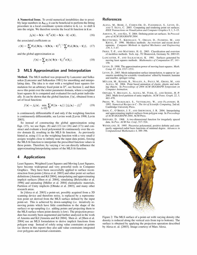
Figure 2: The MLS surface of a point-set with varying density (thedensity is reduced along the vertical axis from top to bottom). Thesurface is obtained by applying the projection operation describedby Alexa et. al. [2003]. Image courtesy of Marc Alexa.