AN EMPIRICAL ANALYSIS OF POVERTY AND INCOME

INEQUALITY IN WEST VIRGINIA

Semoa C. B. De Sousa-Brown, Graduate Research Assistant Tesfa G. Gebremedhin, Professor

Divisison of Resource Management Devis College of Agriculture, Forestry & Consumer Sciences

P.O. Box 6109 West Virginia University

Morgantown, WV 26505-6108

Selected Paper prepared for presentation at the American Agricultural Economics Association Annual Meetings, Denver, Colorado, August 1-4, 2004 Copyright 2004 by Semoa De Sousa-Brown, Tesfa Gebremedhin. All rights reserved. Readers may make verbatim copies of this document for non-commercial purposes by any means, provided that this copyright notice appears on all such copies.

AN EMPIRICAL ANALYSIS OF POVERTY AND INCOME INEQUALITY IN WEST VIRGINIA

ABSTRACT

OLS and 2SLS regressions and cross-sectional county data are used to examine the major determinants of poverty and income inequality in rural counties of West Virginia. The empirical findings confirm the possibility of simultaneity between poverty and income inequality. Poverty is the main determinant of increased levels of income inequality. KEY WORDS: Rural Poverty, Income Inequality

AN EMPIRICAL ANALYSIS OF POVERTY AND INCOME INEQUALITY IN WEST VIRGINIA

INTRODUCTION

West Virginia is second, after Mississippi, in the nation in terms of the incidence

of poverty, and it lags behind the nation and the Appalachian region for most economic

indicators. High rates of poverty, high unemployment rates, low human capital

formation, and population out-migration, especially by young college graduates, are the

general features of rural life in West Virginia (Dilger and Witt, 1994). The slow or

negative growth in income and employment in the state, the population loss and the

disappearance of rural households are both causes and effects of the persistently high

rates of poverty with repercussions for the economic and social well-being of the rural

population, the health of local business, and the ability of the local governments to

provide basic services (Cushing and Rogers, 1996).

In the 1960s and 1970s, the availability of a low-cost, unskilled, and less educated

labor force helped attract manufacturing from urban to rural areas. This seemed to have

resulted in an apparent decline in rural poverty due to growth and economic vitality

brought about by increased employment. However, in the 1980s and 1990s, global

competition and structural changes in the U.S economy plus the rise in high-tech

industries, demanding highly educated workers, made it difficult for rural areas to attract

industries requiring a skilled labor force. Moreover, there has been a disproportionate

coverage of urban poverty in terms of media and research studies. More federal

programs targeted to alleviate poverty have been devoted to urban as compared to rural

areas. The failure of the literature on poverty to adequately address rural poverty limits

its scope in understanding the vitally different character and changing nature of rural

poverty, and hence its value for policy makers in designing development and federal

programs to serve the rural poor (Deavers and Hoppe, 1992).

Poverty is a historical fact of life in many rural areas of America, and the

Appalachian region where West Virginia is located, is a classic example of deeply rooted

poverty. Despite the economic expansion of the late 1980s, rural areas have lagged

behind the rest of the nation, and poverty rates remained high (Deavers and Hoppe,

1992). This evidence suggests that many rural areas and rural poor are at a disadvantage

1

when competing for new job and higher income opportunities, even in a growing

economy. The Appalachian Regional Commission (ARC) has classified 28 percent

(about 111) of the 406 Appalachian counties as distressed due to low per-capita income

plus high poverty and unemployment rates (Allen-Smith et al., 2000). Furthermore, there

is evidence of inequality in the rural areas in general and particularly in rural Appalachia

(both in terms of size distribution of household income, and government funds for

poverty assistance). The causes of poverty are multifaceted and complex (Duncan,

1992). Nevertheless it has been shown that poverty is inextricably linked to the labor

market, income inequalities by race and gender, welfare dependence, single-parent

families, presence of pre-school children, low human capital, lack of earning ability, low

annual earnings, and economic insecurity.

The structural changes in rural economies are not temporary phenomena, but a

situation in which the economic bases of rural communities will be changing constantly

as a response to ongoing international forces and national structural economic

adjustments (Reeder, 1990). To provide public facilities and services, and to strengthen

and diversify the local economy, policy makers and local leaders need to know the

incidence of poverty and the nature of income distribution patterns. Understanding the

characteristics of the rural poor is crucial for designing specific development policies to

attenuate the causes of poverty and alleviate income inequality.

Background Information on West Virginia

West Virginia is part of the Appalachian region, which has relatively high poverty

rates, high unemployment rates, and a low ratio of jobs to people (Allen-Smith et al.,

2000). In West Virginia 32 counties are classified as “transitional,” and 21 counties are

classified as “distressed,” making a total of 53 counties. Forty-three of these 53 counties

are located within rural (non-metropolitan) areas (Appalachian Regional Commission,

1999).2 The state of West Virginia does not have an “attainment” county, and only

Jefferson and Putnam Counties are considered “competitive” counties (Appalachian

2 Distressed counties are those with 1999-2001 three-year average unemployment rate of 6.8 percent or more, 2000 per capita market income of $16,073 or less, and a 2000 Census poverty rate of 19.1 percent or higher. Attained counties are those with 1999-2001 three-year average unemployment rate of 3.8 percent or less, 2000 per capita market income of $25.882 or more, and a 2000 Census poverty rate of 11.2percent or less. Transitional are counties that are not in other class, and individual indicators vary. (ARC, 2001).

2

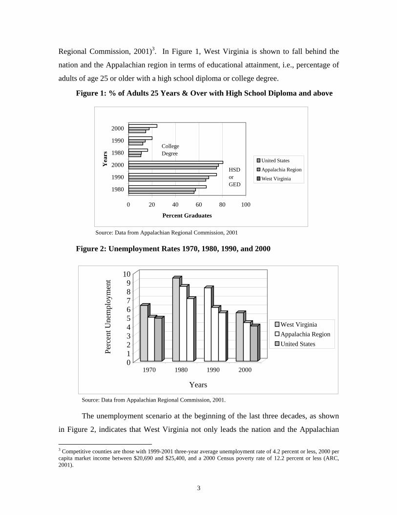
Regional Commission, 2001)3. In Figure 1, West Virginia is shown to fall behind the

nation and the Appalachian region in terms of educational attainment, i.e., percentage of

adults of age 25 or older with a high school diploma or college degree.

Figure 1: % of Adults 25 Years & Over with High School Diploma and above

0 20 40 60 80 100

1980

1990

2000

1980

1990

2000

Yea

rs

Percent Graduates

United States

Appalachia Region

West Virginia

College Degree

HSD or GED

Source: Data from Appalachian Regional Commission, 2001

Figure 2: Unemployment Rates 1970, 1980, 1990, and 2000

0123456789

10

Perc

ent U

nem

ploy

men

t

1970 1980 1990 2000

Years

West VirginiaAppalachia RegionUnited States

Source: Data from Appalachian Regional Commission, 2001.

The unemployment scenario at the beginning of the last three decades, as shown

in Figure 2, indicates that West Virginia not only leads the nation and the Appalachian

3 Competitive counties are those with 1999-2001 three-year average unemployment rate of 4.2 percent or less, 2000 per capita market income between $20,690 and $25,400, and a 2000 Census poverty rate of 12.2 percent or less (ARC, 2001).

3

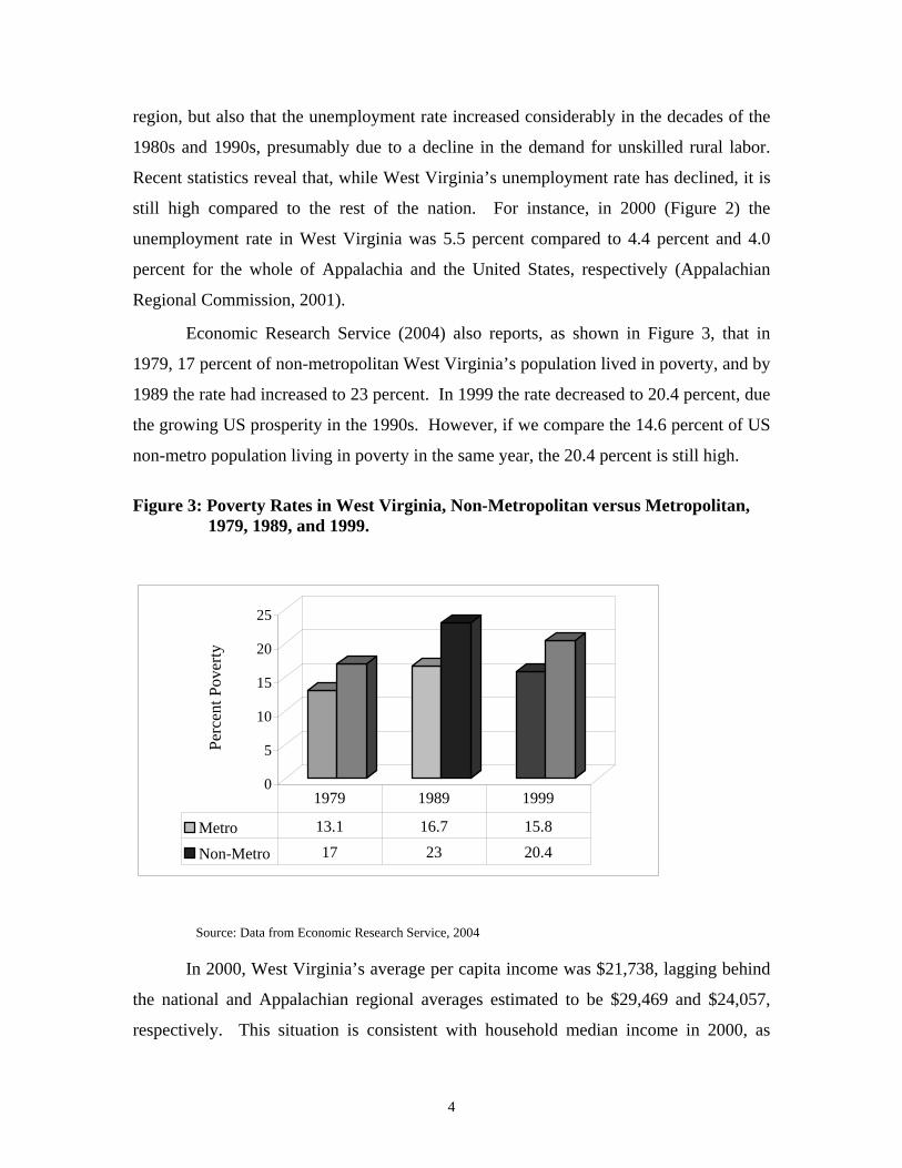
region, but also that the unemployment rate increased considerably in the decades of the

1980s and 1990s, presumably due to a decline in the demand for unskilled rural labor.

Recent statistics reveal that, while West Virginia’s unemployment rate has declined, it is

still high compared to the rest of the nation. For instance, in 2000 (Figure 2) the

unemployment rate in West Virginia was 5.5 percent compared to 4.4 percent and 4.0

percent for the whole of Appalachia and the United States, respectively (Appalachian

Regional Commission, 2001).

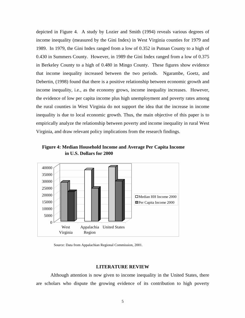
Economic Research Service (2004) also reports, as shown in Figure 3, that in

1979, 17 percent of non-metropolitan West Virginia’s population lived in poverty, and by

1989 the rate had increased to 23 percent. In 1999 the rate decreased to 20.4 percent, due

the growing US prosperity in the 1990s. However, if we compare the 14.6 percent of US

non-metro population living in poverty in the same year, the 20.4 percent is still high.

Figure 3: Poverty Rates in West Virginia, Non-Metropolitan versus Metropolitan, 1979, 1989, and 1999.

0

5

10

15

20

25

Perc

ent P

over

ty

Metro 13.1 16.7 15.8

Non-Metro 17 23 20.4

1979 1989 1999

Source: Data from Economic Research Service, 2004

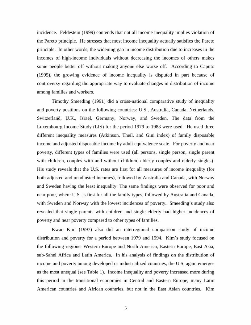
In 2000, West Virginia’s average per capita income was $21,738, lagging behind

the national and Appalachian regional averages estimated to be $29,469 and $24,057,

respectively. This situation is consistent with household median income in 2000, as

4

depicted in Figure 4. A study by Lozier and Smith (1994) reveals various degrees of

income inequality (measured by the Gini Index) in West Virginia counties for 1979 and

1989. In 1979, the Gini Index ranged from a low of 0.352 in Putnan County to a high of

0.430 in Summers County. However, in 1989 the Gini Index ranged from a low of 0.375

in Berkeley County to a high of 0.480 in Mingo County. These figures show evidence

that income inequality increased between the two periods. Ngarambe, Goetz, and

Debertin, (1998) found that there is a positive relationship between economic growth and

income inequality, i.e., as the economy grows, income inequality increases. However,

the evidence of low per capita income plus high unemployment and poverty rates among

the rural counties in West Virginia do not support the idea that the increase in income

inequality is due to local economic growth. Thus, the main objective of this paper is to

empirically analyze the relationship between poverty and income inequality in rural West

Virginia, and draw relevant policy implications from the research findings.

Figure 4: Median Household Income and Average Per Capita Income in U.S. Dollars for 2000

0

5000

10000

15000

20000

25000

30000

35000

40000

WestVirginia

AppalachiaRegion

United States

Median HH Income 2000Per Capita Income 2000

Source: Data from Appalachian Regional Commission, 2001.

LITERATURE REVIEW

Although attention is now given to income inequality in the United States, there

are scholars who dispute the growing evidence of its contribution to high poverty

5

incidence. Feldestein (1999) contends that not all income inequality implies violation of

the Pareto principle. He stresses that most income inequality actually satisfies the Pareto

principle. In other words, the widening gap in income distribution due to increases in the

incomes of high-income individuals without decreasing the incomes of others makes

some people better off without making anyone else worse off. According to Caputo

(1995), the growing evidence of income inequality is disputed in part because of

controversy regarding the appropriate way to evaluate changes in distribution of income

among families and workers.

Timothy Smeeding (1991) did a cross-national comparative study of inequality

and poverty positions on the following countries: U.S., Australia, Canada, Netherlands,

Switzerland, U.K., Israel, Germany, Norway, and Sweden. The data from the

Luxembourg Income Study (LIS) for the period 1979 to 1983 were used. He used three

different inequality measures (Atkinson, Theil, and Gini index) of family disposable

income and adjusted disposable income by adult equivalence scale. For poverty and near

poverty, different types of families were used (all persons, single person, single parent

with children, couples with and without children, elderly couples and elderly singles).

His study reveals that the U.S. rates are first for all measures of income inequality (for

both adjusted and unadjusted incomes), followed by Australia and Canada, with Norway

and Sweden having the least inequality. The same findings were observed for poor and

near poor, where U.S. is first for all the family types, followed by Australia and Canada,

with Sweden and Norway with the lowest incidences of poverty. Smeeding’s study also

revealed that single parents with children and single elderly had higher incidences of

poverty and near poverty compared to other types of families.

Kwan Kim (1997) also did an interregional comparison study of income

distribution and poverty for a period between 1979 and 1994. Kim’s study focused on

the following regions: Western Europe and North America, Eastern Europe, East Asia,

sub-Sahel Africa and Latin America. In his analysis of findings on the distribution of

income and poverty among developed or industrialized countries, the U.S. again emerges

as the most unequal (see Table 1). Income inequality and poverty increased more during

this period in the transitional economies in Central and Eastern Europe, many Latin

American countries and African countries, but not in the East Asian countries. Kim

6

summarizes that although the causes behind interregional disparities are country-specific,

it could be argued that for developed countries it is due to the linkages between the

changes in labor and capital markets within the domestic economy and the global

economy in technology, trade and capital movement, and vice-versa.4 Furthermore, he

asserts that for many developing countries, the rise in inequality and poverty between

1979 and 1994 is due also to the downside of globalization in the context of rapidly

evolving technologies, which increased the demand for better-educated and trained

workers even in developing countries.

Table 1 Quintile Distributions in the OECD Nations during the 1980s

Countries Income Share of The Ratio of Income Share Bottom Quintile % of Bottom to the Top Quintile

France 6.3 6.48Great Britain 5.8 6.81Italy 6.8 6.03Germany 6.8 5.69Japan 8.7 4.31United States 4.7 8.91Average 6.5 6.14Source: Kim, 1997 pp. 1911 (World Bank Data).

In 1996, Alain de Janvry and Elisabeth Sadoulet conducted a causal analysis

study on growth, inequality, and poverty in Latin America. They conducted a detailed

country specific-spells analysis of growth and recession between 1970 and 1994. The

causal relationship between growth rates in inequality represented by the Gini index, the

rate of growth in rural poverty and the rate of growth in urban poverty were determined

simultaneously. They hypothesized that the Gini index is affected by urban and rural

poverty growth rates and that urban poverty growth rates are affected by rural poverty

growth rates, and reciprocally, through the migration rate. The Gini Coefficient affects

both rural and urban poverty growth rates. The results show that when the incidence of

poverty is specified (headcount ratios), poverty has a significant impact on inequality.

When poverty is specified as number of poor, poverty is affected by inequality, but

inequality is not affected by poverty.

4 Vice-versa is in the sense that global economy is also linked to the domestic labor market. According to Kim (1997) the adoption of labor-saving technologies and shift in consumer demands toward technology-

7

Through the set of other explanatory variables, de Janvry and Sadoulet tried to

find the main determinants of inequality, urban and rural poverty. They found that

economic growth was not a strong determinant of changes (increases) in inequality, but

migration was (during the study period). Furthermore, the most important factors that

contributed to decreasing inequality were structural characteristics of the countries, such

as a higher share of agriculture in GDP, or a higher share of urban in total population, and

higher initial income inequality level. For both urban and rural poverty, they found that

economic growth (as measured by GDP per capita) reduced poverty rates, but the effect

was partially cancelled by the fact that growth increases inequality, which in turn

increases poverty. The structural features of the countries also played an important role

in determining changes in poverty. For instance, they found that when countries had

higher initial GDP per capita and higher initial levels of poverty there were greater

reductions in both urban and rural poverty. The authors also tried to determine total

effects of growth and found that for all periods a negative relationship between income

and poverty (both urban and rural) occurred mainly during recessions.

Other important components (besides the labor market and changing

demographics) that have been emerging in recent studies of income inequality and

poverty are race, gender and family structure. Darity et al. (1998) used a decomposition

model on racial earnings disparity and family structure during the end of the Carter

administration and into the Reagan and Bush administrations, and found that gender and

race discrimination explain substantial portions of the gaps in earnings. They assert that,

although family structure matters, racial discrimination (especially pre-labor and labor-

market treatment) was a stronger influential factor in the determination of the widening

racial gaps in earnings among family heads during the shift that began toward the end of

the Carter administration and lasted into the Reagan and Bush administrations (1976-

1985). The authors purport that if blacks and whites were treated equally in every aspect

to the point that the coefficients in the labor force participation, family structure, and

earnings equations were identical for both groups, then there would have been a

convergence of black and white probabilities of female-headed families by 1985, black

intensive products away from standardized products has induced a widening wage gap between skilled and unskilled workers.

8

labor force participation would have climbed, black earnings would have increased

tremendously, and earning disparities would have declined dramatically.

Caputo (1995) also studied the effect of race and the policies of five different

administrations (Nixon, Ford, Carter, Reagan and Bush) on income inequality and family

poverty. The study focused on main effects for the decades of the 1970s and 1980s as

well as race and interaction effects on several family-income dispersion and poverty

measures, including the Gini index and income-poverty ratio. Multivariate and univariate

ANOVAs were used in the study. Caputo’s findings reveal that both black and white

low-income families were worse off in the 1980s than they were in the 1970s due to

different policies intended to alleviate poverty. Furthermore, the gap between high and

low-income black families, which widened considerably in the 1970s, widened even

further in the 1980s compared with their white counterparts (Caputo, 1995). In other

words, low-income black families were pushed further into poverty by having less

income in the 1980s compared with other groups (high and low-income white households

and high-income black households).

At the regional level Ngarambe et al., (1998) examined joint determinants of

southern U.S. county-level income growth and income inequality using Gini coefficients

for decades of the 1970s and 1980s. The study tested for reverse causality between

income growth and income inequality (endogenous variables), using two-stage least

squares regression. Among the list of explanatory variables for the structural model,

were variables such as educational attainment, earnings from the industrial mix per

county, wage, minority, and female-headed households. Their results reveal a positive

relationship between family income growth and income inequality in the 1980s, while in

the 1970s it is not statistically significant (below 10 percent level) in explaining income

inequality. Furthermore, their results confirm the evidence of an increased income

inequality in the 1980s and a positive relationship between the racial factor and income

inequality primarily due to job discrimination and limited economic opportunities, as

reported by other studies. However, the evidence of low per capita income plus high

unemployment and poverty rates among the rural counties in West Virginia does not

support the idea that the increase in income inequality is due to local economic growth

(Ngarambe et al., 1998).

9

Robert Lerman (1996) used shift-share analysis and Gini decomposition methods

to study the impact of the changing U.S. family structure on child poverty and income

inequality. Basically Lerman wanted to examine what would have happened if the

existing unmarried mothers had married the pool of unmarried men and if both men and

women had changed their earnings patterns in response to their new family and income

situations. The Gini decomposition served to capture the inequality within groups and

between groups, and the stratification terms. Then new poverty rates for each group

(black and white) were projected based on the new family structure.

Lerman’s study reveals that family structure changes were of foremost importance

to changes in poverty and income inequality. Lerman asserts that based on his simulated

marriages and marriage-induced earnings effects, the 1971-1989 trend away from

marriage among parents accounted for almost half the rise in income inequality and more

than the entire increase in child poverty rates. Moreover, he affirms that changes in

family structure increased income inequality and poverty among children of both white

and black groups; however, black children were affected more by the weakening ties of

marriages among parents.

West Virginia, Motahar (1986) studied the relationship between alternative

employment mixes and income distribution patterns in the counties for 1970 and 1980.

He found that service-producing industries create more than 60 percent of total

employment in the state, and the highest percentage increase in employment in the

service-producing industries over the decade was in the finance, insurance and real estate

sector. Based on industries that generated highest percentages of total employment,

Motahar identified five different types of counties: mining, non-durable goods

manufacturing, durable goods manufacturing, retail trade, and professional services. The

findings reveal that manufacturing counties had the least income inequality among the

five county types, and professional services counties had the highest income inequality.

Moreover, it was found that the manufacturing sector as a whole tends to have an

equalizing effect on income distribution.

Lozier (1993) studied the relationship between economic growth (measured as

change in total personal income) and income inequality (measured by Gini index) in the

counties of West Virginia for 1989. The hypothesis was that the income inequality level

10

is a function of economic growth. However, Lozier found no evidence to support the

conclusion that economic growth is a determinant of household income inequality.

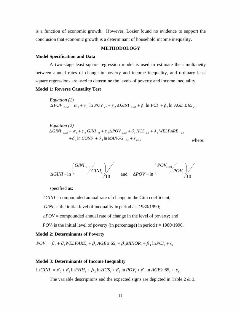
METHODOLOGY

Model Specification and Data

A two-stage least square regression model is used to estimate the simultaneity

between annual rates of change in poverty and income inequality, and ordinary least

square regressions are used to determine the levels of poverty and income inequality.

Model 1: Reverse Causality Test

Equation (1)

tctctctc AGEPCIGINIPOVPOV ,21,210, 65lnlnln ≥++∆++=∆ ∆∆ φφγγα

Equation (2)

tctc

tctctctctc

MANUGCONS

WELFAREHCSPOVGINIGINI

,2,43

,2,1,431,

lnln εδδ

δδγγα

+++

++∆++=∆ ∆∆

where:

10ln10 ⎟

⎠⎞

⎜⎝⎛

=∆

+

t

tGINI

GINI

GINI and 10ln10 ⎟

⎠⎞

⎜⎝⎛

=∆

+

t

tPOV

POV

POV

specified as:

∆GINI = compounded annual rate of change in the Gini coefficient;

GINIt = the initial level of inequality in period t = 1980/1990;

∆POV = compounded annual rate of change in the level of poverty; and

POVt is the initial level of poverty (in percentage) in period t = 1980/1990.

Model 2: Determinants of Poverty

tttttt PCIMINORAGEWELFAREPOV εβββββ +++≥++= ln65 43210

Model 3: Determinants of Income Inequality

tttttt AGEPOVHCSFHHGINI εβββββ +≥++++= 65lnlnlnlnln 43210

The variable descriptions and the expected signs are depicted in Table 2 & 3.

11

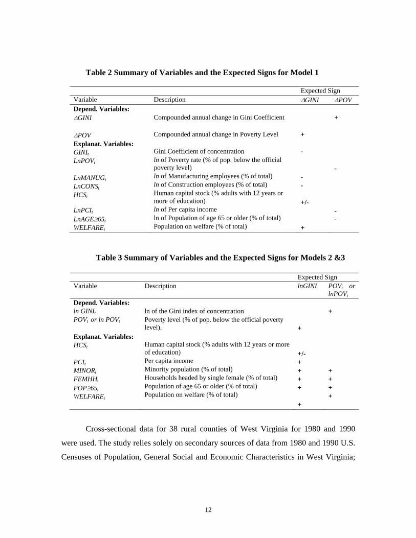
Table 2 Summary of Variables and the Expected Signs for Model 1

Expected Sign Variable Description ∆GINI ∆POV Depend. Variables: ∆GINI ∆POV Explanat. Variables: GINIt

LnPOVt

LnMANUGt

LnCONSt

HCSt LnPCIt

LnAGE≥65t

WELFAREt

Compounded annual change in Gini Coefficient Compounded annual change in Poverty Level Gini Coefficient of concentration ln of Poverty rate (% of pop. below the official poverty level) ln of Manufacturing employees (% of total) ln of Construction employees (% of total) Human capital stock (% adults with 12 years or more of education) ln of Per capita income ln of Population of age 65 or older (% of total) Population on welfare (% of total)

+ - - - +/- +

+ - - -

Table 3 Summary of Variables and the Expected Signs for Models 2 &3

Expected Sign Variable Description lnGINI POVt or

lnPOVt

Depend. Variables: ln GINIt

POVt or ln POVt

Explanat. Variables: HCSt

PCIt

MINORt

FEMHHt

POP≥65t

WELFAREt

ln of the Gini index of concentration Poverty level (% of pop. below the official poverty level). Human capital stock (% adults with 12 years or more of education) Per capita income Minority population (% of total) Households headed by single female (% of total) Population of age 65 or older (% of total) Population on welfare (% of total)

+ +/- + + + + +

+ + + + +

Cross-sectional data for 38 rural counties of West Virginia for 1980 and 1990

were used. The study relies solely on secondary sources of data from 1980 and 1990 U.S.

Censuses of Population, General Social and Economic Characteristics in West Virginia;

12

Regional Economic Information Service (REIS); Bureau of Labor Statistics, and Bureau

of Business and Economic Research of WVU.

RESULTS AND DISCUSSION

The results of the OLS/TSLS regressions (model 1) for 1980 and 1990 are shown

in the Tables 4a and 4b, respectively. The 1980 OLS estimation for the annual rate of

change in poverty levels (equation 1) reveals that the estimated coefficients for the annual

rate of changes in the Gini index (∆GINI), the initial poverty levels, and the proportion of

the population of age 65 or older are statistically significant at less than 1 percent level.

The signs of the first two coefficients conform to the expected signs. The sign of the

coefficient for the proportion of the population age 65 or older is positive, which is

contrary to what was originally hypothesized.

The model explains 49.9 percent of the variation (R2) in the annual rate of change

in poverty levels. The F-statistic for the model was also significant at less than 1 percent

level. The model is correctly specified according to Ramsey’s RESET test F-statistic,

which is lower than that of the model. The Hausman test for simultaneity resulted in

statistically significant residual at less than 1 percent level, thus confirming the

simultaneity between poverty (∆POV) and income inequality (∆GINI). This means that

the endogenous regressor ∆GINI is correlated with the error term; therefore, the TSLS

regression would yield more efficient estimates. As shown in Table 4a, the signs and the

statistical significance of the estimated coefficients remained the same, but the

coefficients and the t-statistics changed with the TSLS. White’s test revealed no presence

of heteroskedasticity.

The TSLS results reveal that a one-percentage increase in the annual rate of

change in the Gini index (income inequality) increased the annual rate of change in

poverty levels by 2.99 percent. A one-percentage increase in the initial poverty level

decreased the annual rate of change in poverty levels (∆POV) by 0.038 percent.

Moreover, as the proportion of the population age 65 or older increased by 1 percent, the

annual rate of change in poverty levels increased by 0.0412 percent. These findings

imply that counties that had higher annual increases in income inequality and higher

percentages of population age 65 or older, experienced higher rates of change in the

annual poverty levels in 1980 compared to those with lower income inequality and less

13

elderly populations. On the other hand, counties that had higher initial poverty levels

experienced decreased annual rates of change in poverty levels.

14

Table 4a Regression Estimates of Reverse Causality Test between Poverty and Income Inequality Specified by equations 1 and 2 (Model 1), 1980

OLS - 1980 TSLS - 1980 Dependent Variables ∆POV ∆GINI ∆POV ∆GINIExplanatory Variables Coefficient Estimates Coefficient EstimatesConstant -0.0262 0.080*** -0.0091 0.0568**

(-0.129) (6.179) (-0.0429) (2.396)

∆POV 0.115*** 0.1624***(5.444) (3.112)

∆GINI 2.850*** 2.99***(4.672) -4.75

lnPOV -0.034*** - 0.038***(-3.157) (-3.849)

lnPCI 0.003 0.001(0.132) (0.0435)

lnAGE 0.038*** 0.0412***(3.112) (2.852)

GINI -0.174*** -0.120**(-5.537) (-2.110)

HCS -0.006*** -0.0063***(-3.730) (-3.201)

WELFARE 0.004 0.0039***(3.497) (2.939)

lnCONS 0.001*** 0.0011(1.175) (0.958)

lnMANUG -0.003*** -0.0024***(-4.535) (-2.918)

R2 0.499 0.814 0.496 0.77

Adjusted R2 0.438 0.779 0.435 0.72

F-statistic 8.208*** 22.69*** 7.98*** 14.82***

Durbin-Watson 2.34 2.25

n 38 38 38

Hausman estimated residual 1.813*** 0.181**(3.111) (2.276)

Ramsey's RESET F-statistics 4.79** 1.32

White's heteroskedasticity χ2 11.29 33.02

Note: *** =< 1% significance level; ** = < 5% significance level; * =< 10% significance level. Numbers in parenthesis are t-statistics.

38

15

Table 4b Regression Estimates of Reverse Causality Test between Poverty and Income Inequality Specified by equations 1 and 2 (Model 1), 1990

OLS - 1990 TSLS - 1990 Dependent Variables ∆POV ∆GINI ∆POV ∆GINIExplanatory Variables Coefficient Estimates Coefficient EstimatesConstant 0.438** 0.002 0.4538** -0.0085

(2.437) (0.349) (2.351) (-0.955)

∆POV 0.012 0.0313**(1.453) (2.197)

∆GINI 5.73 5.846(1.637) (1.661)

lnPOV -0.049*** -0.0501***(-6.403) (-5.543)

lnPCI -0.0467** -0.0484**(-2.430) (-2.348)

lnAGE 0.0626*** 0.0645***(6.307) (5.462)

GINI -0.001 0.0208(-0.101) (1.110)

HCS -0.0005 -0.0006(0.825) (-1.139)

WELFARE 0.0002 0.0003(0.825) (0.765)

lnCONS 0.0001 0.0002(0.697) (0.660)

lnMANUG -0.000006 0.0003(-0.283) (0.844)

R2 0.61 0.153 0.610 -0.0026

Adjusted R2 0.563 -0.011 0.562 -0.1966

F-statistic 12.95*** 0.932 10.20*** 1.147

Durbin-Watson 1.98 2.49

n 38 38 38

Hausman estimated residual -8.111 -0.0022(-0.798) (0.1095)

Ramsey's RESET F-statistics 2.13 5.02**

White's heteroskedasticity χ2 4.47 12.3

Note: *** =< 1% significance level; ** = < 5% significance level; * =< 10% significance level. Numbers in parenthesis are t-statistics.

38

16

The results for the poverty equation (model 1) for 1990 are shown in Table 4b.

The estimation procedures (OLS, Hausman’s test, Ramsey’s RESET test, White’s

heteroskedasticity test, and TSLS) were used for 1990 data. The estimated residual in

Hausman’s test was not statistically significant, thus implying no simultaneity between

poverty (∆POV) and income inequality (∆GINI). However, the TSLS coefficients were

compared with the OLS estimates (Table 4b). The lack of simultaneity between ∆POV

and ∆GINI for 1990 is believed to be associated with the fact that annual rate of change

in the Gini index may be very small between 1990 and 2000.

For 1990 the initial levels of poverty and the proportion of the population of age

65 or older, exhibited the identical sign and the level of significance (at less than the 1

percent level) as it was for 1980. However, for per capita income, although it has the

same sign as initially hypothesized, the coefficient for 1990 is statistically significant at

below the 5 percent level, which was not the case for 1980 (see Tables 4a and 4b). The

annual rate of change in the Gini index (besides the lack of simultaneity) is not

statistically significant. The model explains 61 percent of the variation in the annual

rates of change in poverty levels for 1990 and the F-statistic is significant at less than the

1 percent level. Ramsey’s RESET test confirms that the model is correctly specified as

shown by lower F-statistic compared to that of the model. White’s test reveals no

heteroskedasticity.

The results in Table 4b imply that counties that had initial poverty levels higher

by 1 percent had reduced annual rates of change in poverty levels by 0.049 percent. The

findings indicating that the higher initial poverty levels contributed to reduce the annual

rate of change in poverty levels are consistent with the findings of de Janvry and Sadoulet

(1996) in Latin America. As the proportion of population age 65 or older increased in the

counties by 1 percent, the annual rate of change in poverty levels increased by 0.0626

percent in these counties. The sign of the coefficient of the proportion of population age

65 or older was hypothesized to be negatively related to the changes in annual rate of

poverty. The hypothesis was based on the belief that many elderly population are retired

and, hence, would have higher retirement incomes. However, the results for both 1980

and 1990 imply that in the rural areas of West Virginia the elderly population still is not

very well-to-do despite the fact that various studies report reduced poverty rates among

17

the elderly groups (Deavers and Hoppe, 1992; Ruggles, 1991). It may also be the case

that although there has been a decline in poverty rates for the elderly, their share of the

total population has grown, thus impacting the annual rate of change in poverty levels.

Moreover, the results are consistent with the studies of Rank and Hirschl (1999), and

Smeeding (1991). In studying the likelihood of poverty across Americans’ adult life

span, Rank and Hirschl (1999) found that by age 65 more than half of all Americans

would have experienced a year below poverty line, and by age 85 two thirds would have

experienced poverty at least for a year.

Counties where the per capita income increased by 10 dollars annually had

reduced annual rates of change in poverty levels by 0.0467 percent. If per capita income

measures the economic growth of a county, this finding is also consistent with the

findings of de Janvry and Sadoulet (1996) in Latin America, where increases in the GDP

(representing the economic growth) decreased poverty levels.

The results of the OLS for income inequality, 1980 (equation 2, model 1) are also

shown in Table 4a. The model explains 77.9 percent of the variation in the annual rate of

change in income inequality (∆GINI) and the F-statistic is significant at less than 1

percent level. Ramsey’s RESET test also confirms that the model is correctly specified

given that the F-statistic of 1.32 is much lower than that of the model (22.69). White’s

test revealed no presence of heteroskedasticity, and the Hausman test for simultaneity

confirmed the simultaneity between ∆GINI and ∆POV at less than the 5 percent level

based on the estimated residual (Table 4a). All the estimated coefficients of TSLS

regression exhibited the hypothesized signs. According to the coefficient, counties that

had 1 percent increase in the annual rate of change in poverty levels contributed to

increased rates of change in income inequality (∆GINI) by 0.1624 percent. Counties with

an initial Gini index higher by 1 percent had decreased annual rates of change in income

inequality by 0.12 percent. A one percent increase in the human capital stock of a county

contributed to reduce the annual rate of change in income inequality by 0.0063 percent.

This implies that education served to equalize economic opportunity and facilitate labor

mobility as discussed by Bishop et al. (1992), and Danzigler and Gottschalk (1993). As

the proportion of people on welfare in a county increased by 1 percent, the annual rate of

change in income inequality increased by 0.0039 percent.

18

Regarding the shares of private employment by industry (construction and

manufacturing), only the coefficient for the manufacturing industry was significant at less

than 1 percent level. This result implies that as the employment shares in manufacturing

industry increase by 1 percent in a county, the annual rate of change in income inequality

decreases by 0.0024 percent. The result is consistent with the findings of Ryscavage and

Henle (1990), and Motahar (1986).

The results for the 1990 income inequality (equation 2, model 1) are also shown

in Table 4b. Starting with the OLS estimation, none of the estimated coefficients were

statistically significant. The model poorly explains the variation in the annual rate of

change in income inequality for 1990, and the Ramsey’s RESET test confirms that the

data does not fit the model. The Hausman test also failed to show simultaneity between

income inequality (∆GINI) and poverty (∆POV) for 1990. Despite the failure of

simultaneity test the TSLS regression was estimated and the same poor results were

observed with the exception that ∆POV was statistically significant at less than 5 percent

level.

Determinants of Poverty

The coefficients for model 2, the poverty model for 1980 and 1990 are shown in

Table 5. Model 2 explains 97.2 percent of the variation in poverty levels in 1980, and the

F-statistic is highly significant at less than 1 percent level (Table 5). Ramsey’s RESET

test confirms that the model is correctly specified, and the χ2 from White’s test indicates

no presence of heteroskedasticity. For 1980, the coefficients for the proportion of the

population on welfare is statistically significant at less than the 1 percent level, as

expected. The coefficient for the proportion of minority population is statistically

significant at less than the 10 percent level, but the negative sign is not as originally

hypothesized and not consistent with other studies at national and regional levels. The

results imply that counties where the proportion of people on welfare increased by 1

percent, poverty level increased by 1.08 percent. On the other hand, counties where the

proportion of minority population increased by 1 percent, poverty level decreased by

0.024 percent. This finding implies that the minority population in rural counties of West

Virginia may be younger and perhaps with a socio-economic level better than those

found in the Black belt or other pockets of poverty around the nation where there are

19

large minority populations. Moreover, in a population with a relatively low average

education, the presence of a small minority group generally will not influence the poverty

level very much.

For 1990, the same model explains 98.8 percent of the variation in poverty levels,

and the F-statistic is highly significant at less than the 1 percent level. Ramsey’s RESET

test indicates that the model is correctly specified, but White’s test indicates the presence

of heteroskedasticity. Before correcting for heteroskedasticity, the coefficient estimates

of the proportion of the population age 65 or older was statistically significant at less than

by 5 percent level, and the coefficient for the proportion of the population on welfare was

statistically significant at less than by 1 percent level. After correcting for

heteroskedasticity, the coefficient estimates for the proportion of the population on

welfare remained statistically significant at less than 1 percent level, while the statistical

significance of the proportion of the population age 65 or older improved from the 5

percent to 1 percent level. The results imply that when the proportion of the population

on welfare increases by 1 percent, an increase of 0.966 percent in poverty levels occurs.

Furthermore, counties that had an increase of 1 percent in the proportion of the

population age 65 or older experienced increased poverty levels by 0.124 percent. This

means that the proportion of population age 65 or older not only affects the annual rate of

change in poverty levels, but it also affects the actual levels of poverty.

20

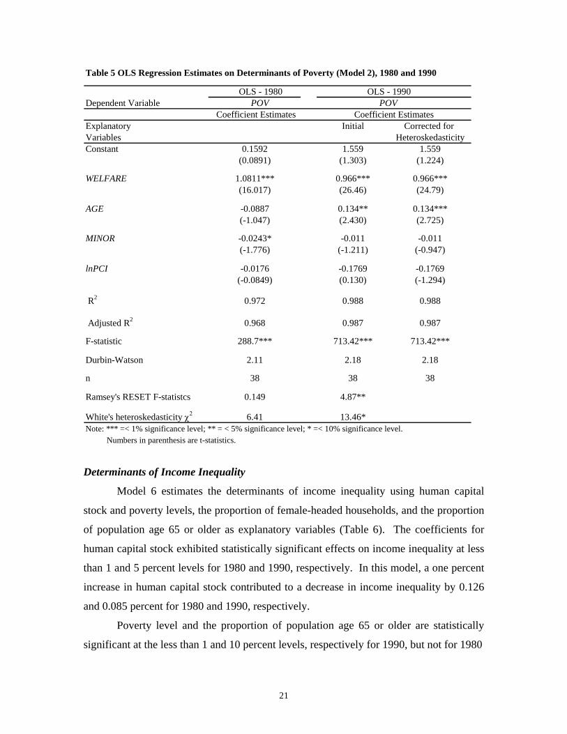
Table 5 OLS Regression Estimates on Determinants of Poverty (Model 2), 1980 and 1990

OLS - 1980 OLS - 1990Dependent Variable POV POV

Coefficient Estimates Coefficient EstimatesExplanatory Initial Corrected for Variables HeteroskedasticityConstant 0.1592 1.559 1.559

(0.0891) (1.303) (1.224)

WELFARE 1.0811*** 0.966*** 0.966***(16.017) (26.46) (24.79)

AGE -0.0887 0.134** 0.134***(-1.047) (2.430) (2.725)

MINOR -0.0243* -0.011 -0.011(-1.776) (-1.211) (-0.947)

lnPCI -0.0176 -0.1769 -0.1769(-0.0849) (0.130) (-1.294)

R2 0.972 0.988 0.988

Adjusted R2 0.968 0.987 0.987

F-statistic 288.7*** 713.42*** 713.42***

Durbin-Watson 2.11 2.18 2.18

n 38 38

Ramsey's RESET F-statistcs 0.149 4.87**

White's heteroskedasticity χ2 6.41 13.46*Note: *** =< 1% significance level; ** = < 5% significance level; * =< 10% significance level. Numbers in parenthesis are t-statistics.

38

Determinants of Income Inequality

Model 6 estimates the determinants of income inequality using human capital

stock and poverty levels, the proportion of female-headed households, and the proportion

of population age 65 or older as explanatory variables (Table 6). The coefficients for

human capital stock exhibited statistically significant effects on income inequality at less

than 1 and 5 percent levels for 1980 and 1990, respectively. In this model, a one percent

increase in human capital stock contributed to a decrease in income inequality by 0.126

and 0.085 percent for 1980 and 1990, respectively.

Poverty level and the proportion of population age 65 or older are statistically

significant at the less than 1 and 10 percent levels, respectively for 1990, but not for 1980

21

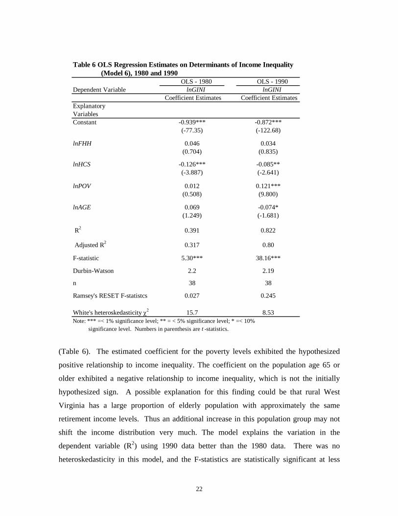
Table 6 OLS Regression Estimates on Determinants of Income Inequality (Model 6), 1980 and 1990

OLS - 1980 OLS - 1990Dependent Variable lnGINI lnGINI

Coefficient Estimates Coefficient EstimatesExplanatoryVariablesConstant -0.939*** -0.872***

(-77.35) (-122.68)

lnFHH 0.046 0.034(0.704) (0.835)

lnHCS -0.126*** -0.085**(-3.887) (-2.641)

lnPOV 0.012 0.121***(0.508) (9.800)

lnAGE 0.069 -0.074*(1.249) (-1.681)

R2 0.391 0.822

Adjusted R2 0.317 0.80

F-statistic 5.30*** 38.16***

Durbin-Watson 2.2 2.19

n 38 38

Ramsey's RESET F-statistcs 0.027 0.245

White's heteroskedasticity χ2 15.7 8.53Note: *** =< 1% significance level; ** = < 5% significance level; * =< 10% significance level. Numbers in parenthesis are t -statistics.

(Table 6). The estimated coefficient for the poverty levels exhibited the hypothesized

positive relationship to income inequality. The coefficient on the population age 65 or

older exhibited a negative relationship to income inequality, which is not the initially

hypothesized sign. A possible explanation for this finding could be that rural West

Virginia has a large proportion of elderly population with approximately the same

retirement income levels. Thus an additional increase in this population group may not

shift the income distribution very much. The model explains the variation in the

dependent variable (R2) using 1990 data better than the 1980 data. There was no

heteroskedasticity in this model, and the F-statistics are statistically significant at less

22

than the 1 percent level. Ramsey’s RESET test indicated no error in the model

specification.

SUMMARY AND CONCLUSIONS

A two-stage least squares regression is applied to estimate the simultaneity

between annual rates of change in poverty and income inequality, and ordinary least

squares regressions are used to examine the determinants of both poverty and income

inequality. Cross-sectional data for 38 rural counties of West Virginia for 1980 and 1990

were used in the study. The econometric results reveal simultaneity between the annual

rate of change in poverty levels and the annual rate of change in income inequality

(represented by the Gini index). Thus, a reverse casual relationship exists between

poverty and income inequality. The results also reveal that initial higher levels of

poverty and income inequality contribute to reduce the compounded annual rate of

change in both poverty and income inequality, respectively. Regarding the determinants

of poverty and income inequality, the econometric results reveal that increases in the

proportions of population on welfare and of the population age 65 or older, contributed to

increase poverty levels (measured as the proportion of people with total incomes below

the official poverty line). On the other hand, increases in the level of per capita income

in the counties contribute to reduce poverty. The main factor that contributes to increase

income inequality, according to the results, is poverty level of the counties. However, the

proportion of human capital stock (represented by percentage of adults of age 25 or older

with high school diploma and/or college degree), tends to reduce income inequality.

Policy Implications

By virtue of exploring the possibility of simultaneity between the two factors, the

study contributes a new perspective on the analysis of poverty and income inequality in

the rural counties of West Virginia. The fact that the annual rates of change in poverty

and income inequality can take place simultaneously helps bring awareness to local

governments and policy makers of the need to design policies and strategies that could

both reduce poverty and income inequality. Generally most poverty reduction strategies

tend to reduce income inequality slightly, however, the strategies to reduce income

inequality do not necessarily reduce poverty. For instance, a strategy to reduce income

23

inequality requires simultaneous interventions to promote job creation and

entrepreneurship as well as to improve equity in the opportunity of participation in these

jobs through improved educational levels. There is also a need to improve access to these

new jobs by reducing gender, wage, and class discrimination that exist in local labor

markets.

The study reveals that higher per capita income is associated with reduced

poverty. The educational attainment reduces income inequality (through the equalizing

effect of economic opportunity). The creation of new jobs may motivate investment in

human capital for males and females, resulting in higher educational attainment, which in

turn results in higher productivity and wages and higher per capita income, leading to less

poverty and income inequality. There is also a need for strategies that would help

upgrade workforce skills and facilitate a long-term transition of welfare recipients into

the workforce, as the study reveals that this group contributes to increased levels of

poverty.

The limitations of this study are with respect to the secondary data used. The lack

of annual data prevented the possibility of combining time-series and cross-section

analyses, which could have made it possible to conduct a comparative analysis of poverty

and income inequality during the recession and recovery periods. The lack of data on in-

kind income and tax obligations and household expenditures at the county level

prevented the calculation of inequality in household expenditures. There may also be the

presence of spatial dependence among the observations. The counties are close to each

other and many share borders, thus the socio-economic conditions in one county may not

differ very much from an immediate neighboring county. Although, the possibility of

spatial dependence is acknowledged, attempts to correct that are beyond the scope of this

study.

24

REFERENCES

Allen-Smith, Joyce E., Ronald C. Wimberley, and Libby V. Morris. “America’s Forgotten People and Places: Ending the Legacy of Poverty in the Rural South.” Journal of Agricultural and Applied Economics, 32:2:319-329, August 2000.

Appalachian Regional Commission, “General Economic Indicators of the Appalachian Region.” Appalachian Regional Commission, 1999.

----------------“Regional Data Results – County Economic Status, Fiscal Year 2004: West Virginia.” www.arc.org. Visited May 11th 2004.

Bishop, J.A., J.P. Formby, and P.D. Thistle. “Explaining Interstate Variation in Income

Inequality.” Review of Economics and Statistics, 74:553-57, 1992. Bureau of Business and Economic Research. “West Virginia: A 20th Century Perspective on

Population Change.” College of Business and Economics, West Virginia University, 1999.

Caputo, Richard K. “Income Inequality and Family Poverty.” Families in Society: The Journal of

Contemporary Human Services, 76: 604-15, 1995. Cushing, Brian and Cyntia Rogers. “Income and Poverty in Appalachia.” Socio-Economic

Review of Appalachia (Papers commissioned by the Appalachia Regional Commission), Regional Research Institute, West Virginia University, 1996.

Economic Research Service (ERS), United States Department of Agriculture, 2004. www.usda.gov/. Visited May 11th 2004.

Danziger, S., and P. Gottschalk. Uneven Tides: Rising Inequality in America. New York: Russel

Sage Foundation, 1993. Darity, Willian A. Jr., Samuel L. Myers, Jr., and Chanjin Chung. “Racial Earnings Disparity and

Family Structure.” Southern Economic Journal, 65(1): 20-41, 1998. De Janvry, Alain and Elisabeth Sadoulet. “Growth, Inequality, and Poverty in Latin America: A

Casual Analysis, 1970-94.” Working Paper N0. 784. Department of Agricultural and Resource Economics, Division of Agriculture and Natural Resources. University of California at Berkeley, 1996.

Deavers, Kenneth L., and Robert A. Hoppe. “Overview of the Rural Poor in the 1980s”; pp. 3-20.

In Cynthia Duncan (ed). Rural Poverty in America. Westport CT: Auburn House, Greenwood Publishing Group, Inc., 1992.

Dilger, Robert Jay and Tom Stuart Witt. “West Virginia’s Economic Future.” pp. 3-15. In

Dilger, Robert Jay and Tom Stuart Witt (eds). West Virginia in the 1990’s: Opportunities for Economic Progress. Morgantown, WV.: West Virginia University Press, 1994.

Duncan, Cynthia. “Persistent Poverty in Appalachia: Scarce Work and Rigid Stratification,”

pp.111-133. In Cynthia Duncan (ed). Rural Poverty in America. Westport CT: Auburn House, Greenwood Publishing Group, Inc., 1992.

25

Feldstein, Martin. “Reducing Poverty, not Inequality.” The Public Interest, 137: 32-41, Fall 1999. Kim, Kwan S. “Income Distribution and Poverty: An Interregional Comparison.” World

Development, 25:11: 1909-24, 1997. Lerman, Robert I. “The Impact of Changing U.S. Family Structure on Child Poverty and Income

Inequality.” Economica, 63:119-139, May 1996. Lozier, J. and D.K. Smith. Household Income Inequality and Economic Change in West Virginia

by County, 1979-1989. R.M. Publication No. 94/2. Division of Resource Management, West Virginia University, 1994.

Lozier, John. Inequality and Economic Growth in West Virginia Counties. M.S. Thesis, Division

of Resource Management, West Virginia University, Morgantown, WV, 1993. Motahar, S.A. An Analysis of the Relationship between Income Distribution and Employment

Mixes by County in West Virginia. M.S. Thesis, West Virginia University, Morgantown, WV, 1986.

Ngarambe`, O., S.J. Goetz, and D.L. Debertin. “Regional Economic Growth and Income Distribution: County Level-Evidence from the U.S. South.” Journal of Agricultural and Applied Economics, 30: 325-337, 1998.

Rank, M.R. and T.A. Hirschl. “The Likelihood of Poverty Across American Adult Life Span”.

Social Work, 44:3: 201-16, May 1999. Reeder, Richard J. Targeting Aid to Distressed Rural Areas (Indicators of Fiscal and Community

Well-being). Staff Report No. AGES 9067, Washington, D.C: USDA/ERS/ARED, 1990. Ryscavage, P., and P. Henle. “Earnings Inequality Accelerates in the 1980s.” Monthly Labor

Review, pp.4-14, December 1990. Smeeding, Timothy M. “Cross-National Comparisons of Inequality and Poverty.” In Lars

Osberg (eds). Economic Inequality and Poverty: International Perspectives. Armonk, New York and London M.E. Sharpe, Inc., 1991.

U.S. Regional Economic Information System (REIS). “Household Income Distribution by

County for 1997.” Washington DC: U.S. Government Printing, 1997. U.S. Census Bureau, “Characteristics of the Population: US Summary.” Census of Population.

Washington DC.: U.S. Government Printing, 1980 and 1990. --------------“General Social and Economic Characteristics, West Virginia.” Census of

Population. Washington DC.: U.S. Government Printing, 1980 and 1990

26