an economic impact study of lower great miami river ... design and art direction: kevin pease, ......

An Economic Impact Study

of Lower Great Miami River

Segment Improvements

Sponsored by:

An Economic Impact Study

of Lower Great Miami River

Segment Improvements

sustaining a

River

Radha Ayalasomayajula

Fred Hitzhusen, PhD.

Pierre Wilner Jeanty

sustaining a

RiverAn Economic Impact Study of Lower Great Miami River Segment Improvements

Radha AyalasomayajulaResearch Associate

Rivers Unlimited

Fred Hitzhusen, PhD.Professor & Research Associate

Dept of Agricultural, Environmental and Development Economics

The Ohio State University

Pierre Wilner JeantyResearch Associate and PhD. Candidate

Dept of Agricultural, Environmental and Development Economics

The Ohio State University

Sponsored by

© 2003 Rivers Unlimited

All rights reserved. No part of this work covered by copyrights hereon may be

reproduced or used in any form or by any means – graphic, electronic, or

mechanical, including photocopying, recording, taping of information on storage

retrieval systems – without the prior written permission of River’s Unlimited.

Layout, Design and Art Direction: Kevin Pease, Serendipity Design

(www.SerendipityDesign.com)

Cover Photograph: The Great Miami River between Troy

and Middletown Ohio by Marilyn Wall

River quotations used in section beginnings © by their respective authors

and courtesy of:

http://www.outdoorclub.org/wilderness_Quotes.html

http://www.quotegarden.com

Acknowledgements

To Mike Fremont, President of Rivers Unlimited for having

initiated the project, and bringing financial support to it.

To the board members of Friends of Great Miami, and Director

Rob Sanders for arranging meetings with the local county

commissioners, township trustees, interest groups and conservation

agencies; for arranging a canoe float on the Great Miami River for

a first hand experience on the nature of the river.

To Bernie Fiedeldey, township trustee of Colerain Township,

and his wife Jo Ann Fiedeldey, for their support.

To the County Auditors’ and Engineers’ Offices of Butler and

Hamilton Counties for facilitating and providing data on properties

and maps.

To the Miami Conservancy District, and Sarah Hippensteel in

particular, for helping us with the surveys.

To the people residing in the Great Miami River corridor for

providing responses to our questionnaires.

To Mark Muse, from the University of Cincinnati, who helped

us in collecting data as part of his internship program.

To Professor Mike Miller, University of Cincinnati for providing

us with valuable information on gravel mining.

Phot

o by

Mar

ilyn

Wal

lP

hot

o by

Mar

ilyn

Wal

l

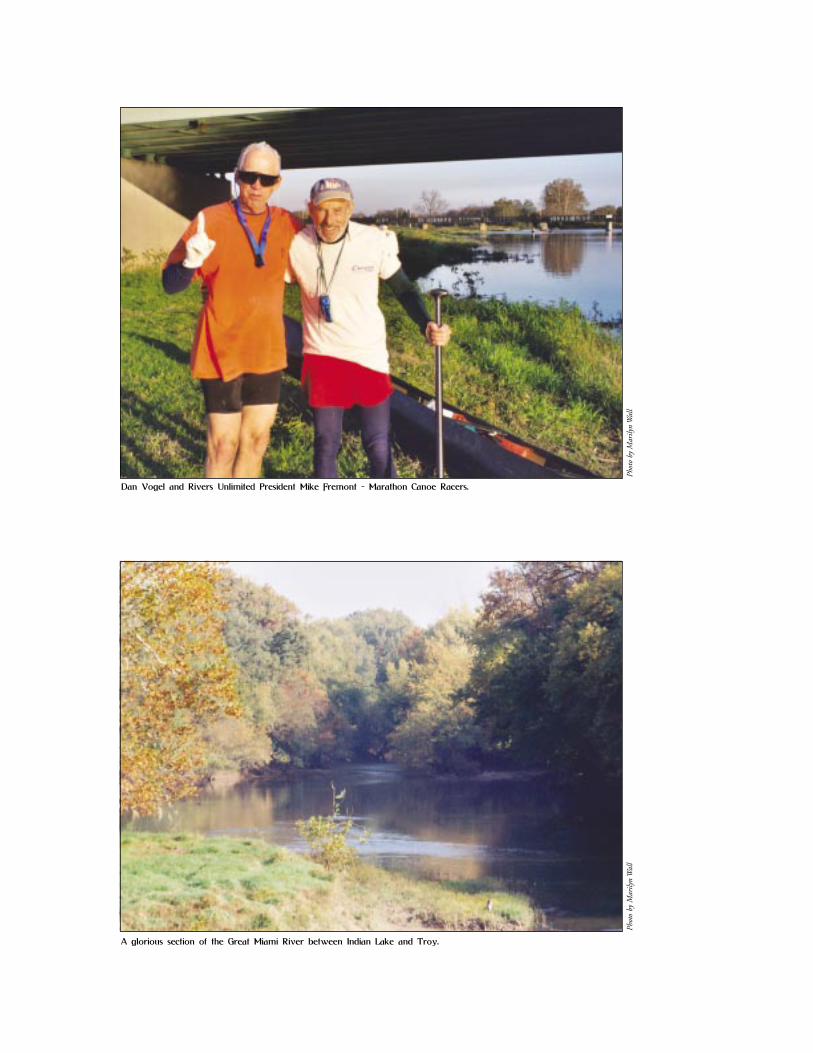
Dan Vogel and Rivers Unlimited President Mike Fremont - Marathon Canoe Racers.

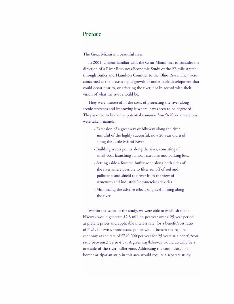
A glorious section of the Great Miami River between Indian Lake and Troy.

Preface

The Great Miami is a beautiful river.

In 2001, citizens familiar with the Great Miami met to consider the

direction of a River Resources Economic Study of the 27-mile stretch

through Butler and Hamilton Counties to the Ohio River. They were

concerned at the present rapid growth of undesirable development that

could occur near to, or affecting the river, not in accord with their

vision of what the river should be.

They were interested in the costs of protecting the river along

scenic stretches and improving it where it was seen to be degraded.

They wanted to know the potential economic benefits if certain actions

were taken, namely:

· Extension of a greenway or bikeway along the river,

mindful of the highly successful, now 20 year old trail,

along the Little Miami River.

· Building access points along the river, consisting of

small-boat launching ramps, restrooms and parking lots.

· Setting aside a forested buffer zone along both sides of

the river where possible to filter runoff of soil and

pollutants and shield the river from the view of

structures and industrial/commercial activities.

· Minimizing the adverse effects of gravel mining along

the river.

Within the scope of the study, we were able to establish that a

bikeway would generate $2.8 million per year over a 25-year period

at present prices and applicable interest rate, for a benefit/cost ratio

of 7.21. Likewise, three access points would benefit the regional

economy at the rate of $740,000 per year for 25 years at a benefit/cost

ratio between 3.32 to 4.57. A greenway/bikeway would actually be a

one-side-of-the-river buffer zone. Addressing the complexity of a

border or riparian strip in this area would require a separate study.

Gravel operations along the river degrade residential values within

one mile of a gravel plant by an average of $16,000, with significant

effects on tax base, a decrease of $2.8 million as loss to the resource

base, and hence, a loss to the local governments in the form of tax

revenues, amounting to more than $100,000 per year.

This is the latest of several River Resource Economics studies at the

Ohio State University sponsored by Rivers Unlimited since 1997. (See

our website at www.RiversUnlimited.org) This version of the study

differs from the original in being more compact, direct and citizen

comprehensible. The original is in the language and format for

professional economists, has been peer reviewed and will be published

in economic journals.

The threat of adverse development is real. The Great Miami is on

the Nationwide Inventory of Rivers as technically qualified, in this

stretch, to be named a National Wild and Scenic River. Only 11,000

miles of rivers (out of 3,500,000 miles) in our country have been so

designated (3/10ths of 1 percent) – in 35 years of the National Wild

and Scenic Rivers Act.

If the Great Miami becomes degraded it could lose this highly

valuable status.

Mike Fremont,

Cincinnati, August 2003

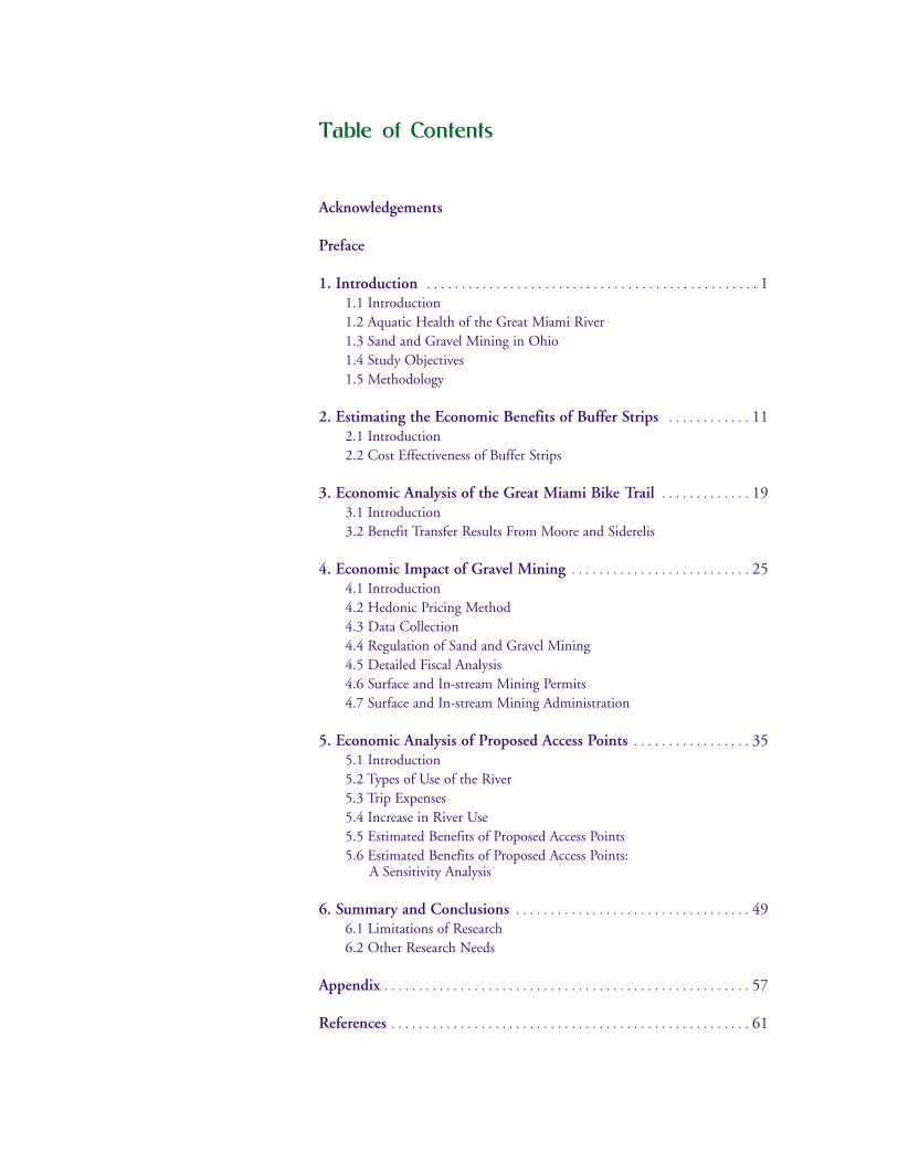
Table of Contents

Acknowledgements

Preface

1. Introduction . . . . . . . . . . . . . . . . . . . . . . . . . . . . . . . . . . . . . . . . . . . . . . . . 1

1.1 Introduction

1.2 Aquatic Health of the Great Miami River

1.3 Sand and Gravel Mining in Ohio

1.4 Study Objectives

1.5 Methodology

2. Estimating the Economic Benefits of Buffer Strips . . . . . . . . . . . . 11

2.1 Introduction

2.2 Cost Effectiveness of Buffer Strips

3. Economic Analysis of the Great Miami Bike Trail . . . . . . . . . . . . . 19

3.1 Introduction

3.2 Benefit Transfer Results From Moore and Siderelis

4. Economic Impact of Gravel Mining . . . . . . . . . . . . . . . . . . . . . . . . . . 25

4.1 Introduction

4.2 Hedonic Pricing Method

4.3 Data Collection

4.4 Regulation of Sand and Gravel Mining

4.5 Detailed Fiscal Analysis

4.6 Surface and In-stream Mining Permits

4.7 Surface and In-stream Mining Administration

5. Economic Analysis of Proposed Access Points . . . . . . . . . . . . . . . . . 35

5.1 Introduction

5.2 Types of Use of the River

5.3 Trip Expenses

5.4 Increase in River Use

5.5 Estimated Benefits of Proposed Access Points

5.6 Estimated Benefits of Proposed Access Points:A Sensitivity Analysis

6. Summary and Conclusions . . . . . . . . . . . . . . . . . . . . . . . . . . . . . . . . . . 49

6.1 Limitations of Research

6.2 Other Research Needs

Appendix . . . . . . . . . . . . . . . . . . . . . . . . . . . . . . . . . . . . . . . . . . . . . . . . . . . . . 57

References . . . . . . . . . . . . . . . . . . . . . . . . . . . . . . . . . . . . . . . . . . . . . . . . . . . . 61

Phot

o by

Mar

ilyn

Wal

l

Eventually, all things

merge into one,

and a river runs through it.

-Norman Maclean, A River Runs Through It

Section 1

Introduction

1

1.1 Introduction

The Great Miami River Watershed is located in the southwest region of Ohio.

This system includes the Great Miami, Stillwater, Whitewater and Mad Rivers.

The drainage area of these systems in Ohio is 4,277 square miles. Total drainage area

including that part in Indiana is 5,702 square miles.

The Great Miami River is 155 miles in length, and its watershed includes all or part

of 15 counties with the headwaters in Hardin and Auglaize counties and the mouth in

the Ohio River in Hamilton County. Interstates 70 and 75, two of the nation’s longest

Interstate highway systems, intersect just north of Dayton. Dayton, with a population

of 190,000, is the largest city within the watershed. Other major cities within the

watershed exceeding 50,000 populations include Springfield, Hamilton and

Middletown. Cities with more than 20,000 people include Piqua, Troy and Fairfield.

Each of these major population centers is located adjacent to one of the waterways in

the watershed.

Some of the most significant water resource features in the watershed are the

Stillwater State Scenic River, the Great Miami buried valley aquifer, the five major

dams (dry) and flood protection system of Miami Conservancy District (MCD), and

Indian Lake, a remnant of the Miami-Erie Canal system and one of the largest lakes

in Ohio. Others are the C.J. Brown Reservoir and Brookville Lake on the Whitewater

River in Indiana.

The Stillwater River above Englewood Dam and Greenville Creek has been

designated a State Scenic River. There are 2,360 miles of rivers and streams in the Great

Miami River Watershed. Water quality in the watershed’s rivers and streams has shown

strong improvement over the last 20 years. The following tables (1.1-1.5) provide

attainment data of WWH (warm water habitat) and EWH (exceptional water habitat)

use designators collected by Ohio EPA (1997) in its stream surveys:

3

An Economic Impact Study of Lower Great Miami River Segment Improvements

Table 1.1Attainment of WWH and EWH Designators for the Watershed in 1995

Attainment Miles

Full 427.3

Threatened 40.3

Partial 309.5

Non-Attainment 285.3

Total Miles Assessed 1063.0

Sustaining a River

4

Table 1.3Attainment of WWH and EWH Designators for the Segment Between Dayton & Middletown

Attainment Year 1980 Year 1989 Year 1995

Full 1.6 miles 6.6 miles 29.9 miles

Partial 3.6 miles 20.7 miles 3.6 miles

Non-Attainment 29.8 miles 7.7 miles 1.5 miles

The improvements in water quality correspond to substantial reductions in the

loadings of oxygen demanding wastes, ammonia-N, and other substances discharged by

point sources. The most significant improvement occurred in the segment between

Dayton and Middletown due to the improved treatment of sewage by the county and

municipal wastewater treatment plants (Ohio EPA 1997).

Table 1.2Attainment of WWH & EWH Designators for the Lower & Middle Great Miami River





Table 1.4Attainment of WWH and EWH Designators for the Segment Between Middletown to Hamilton





Table 1.5Attainment of WWH and EWH Designators for the Segment Between Hamilton & Ohio River





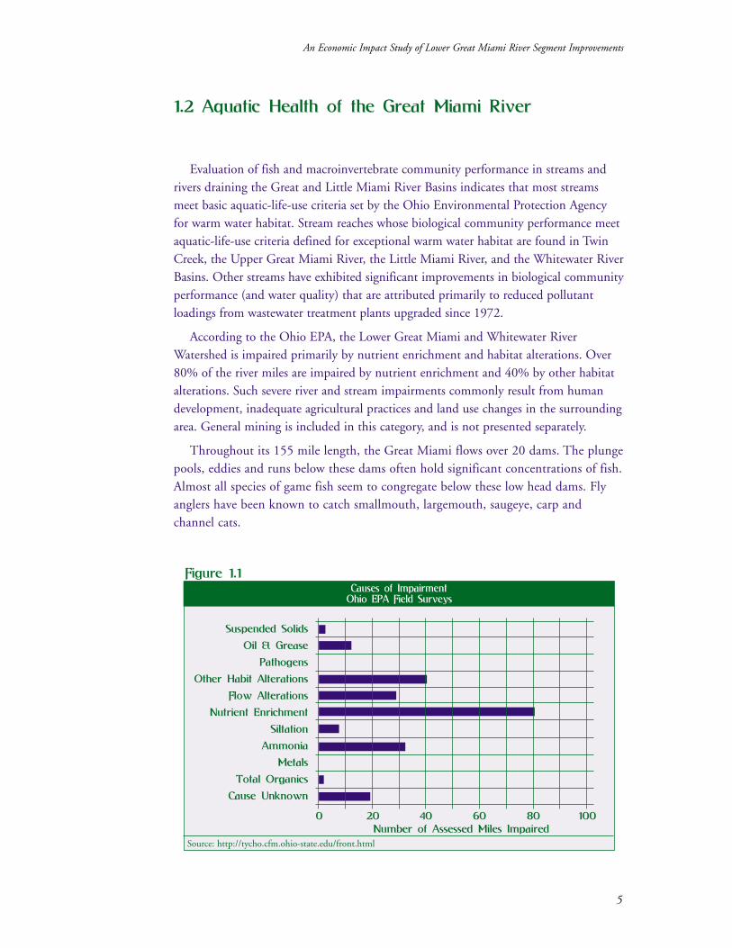
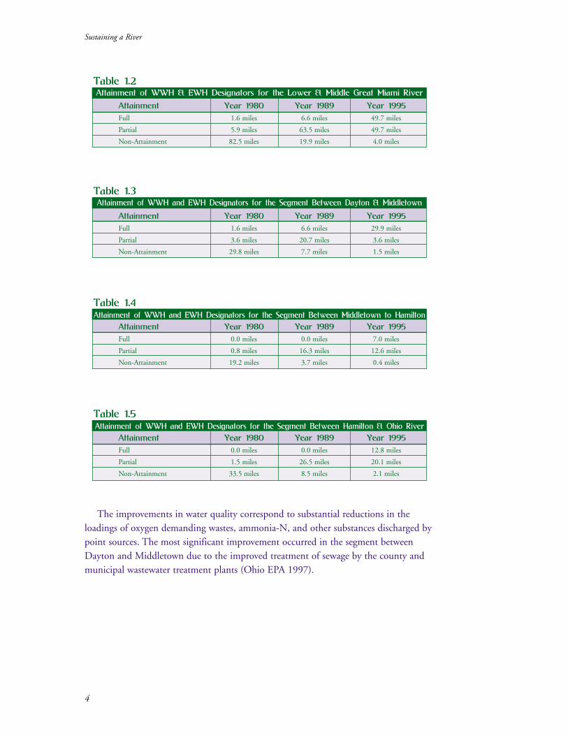
Figure 1.1Causes of Impairment

Ohio EPA Field Surveys

Suspended Solids

Oil & Grease

Pathogens

Other Habit Alterations

Flow Alterations

Nutrient Enrichment

Siltation

Ammonia

Metals

Total Organics

Cause Unknown

0 20 40 60 80 100Number of Assessed Miles Impaired

1.2 Aquatic Health of the Great Miami River

Evaluation of fish and macroinvertebrate community performance in streams and

rivers draining the Great and Little Miami River Basins indicates that most streams

meet basic aquatic-life-use criteria set by the Ohio Environmental Protection Agency

for warm water habitat. Stream reaches whose biological community performance meet

aquatic-life-use criteria defined for exceptional warm water habitat are found in Twin

Creek, the Upper Great Miami River, the Little Miami River, and the Whitewater River

Basins. Other streams have exhibited significant improvements in biological community

performance (and water quality) that are attributed primarily to reduced pollutant

loadings from wastewater treatment plants upgraded since 1972.

According to the Ohio EPA, the Lower Great Miami and Whitewater River

Watershed is impaired primarily by nutrient enrichment and habitat alterations. Over

80% of the river miles are impaired by nutrient enrichment and 40% by other habitat

alterations. Such severe river and stream impairments commonly result from human

development, inadequate agricultural practices and land use changes in the surrounding

area. General mining is included in this category, and is not presented separately.

Throughout its 155 mile length, the Great Miami flows over 20 dams. The plunge

pools, eddies and runs below these dams often hold significant concentrations of fish.

Almost all species of game fish seem to congregate below these low head dams. Fly

anglers have been known to catch smallmouth, largemouth, saugeye, carp and

channel cats.

5


Source: http://tycho.cfm.ohio-state.edu/front.html

The Great Miami buried valley aquifer consists of ancient river valleys filled with

permeable deposits of sand and gravel capable of storing vast amounts of

groundwater. The buried valley aquifer has sustainable yields of 500 to 3,000 gallons

per minute. This aquifer system was designated by the U.S. EPA as a ‘Sole Source

Aquifer’ in 1988. An estimated 97% of the population in the watershed relies on

groundwater for their drinking water supply. The Great and Little Miami River

Basins drain approximately 7,354 square miles in southwestern Ohio and

southeastern Indiana and are included in the more than 50 major river basins and

aquifer systems selected for water-quality assessment as part of the U.S. Geological

Survey’s National Water-Quality Assessment Program.

Land-use and waste-management practices influence the quality of water found in

streams and aquifers in the Great and Little Miami River Basins. Land use is

approximately 79 percent agriculture, 13 percent urban (residential, industrial, and

commercial), and 7 percent forest. An estimated 2.8 million people live in the Great

and Little Miami River Basins; major urban areas include Cincinnati and Dayton,

Ohio. Fertilizers and pesticides associated with agricultural activity, discharges from

municipal and industrial wastewater-treatment and thermoelectric plants, urban runoff,

and disposal of solid and hazardous wastes contribute contaminants to surface water

and ground water throughout the area.

Following the Clean Water Act of 1972 national regulators shut down dirty

industries and other easily identifiable, point-source polluters. Now they are focusing

on less easily managed pollutants, including the sediment dredged up by gravel mines

and runoff from developed areas and farm fields.

Sustaining a River

6

Phot

o by

Mar

ilyn

Wal

l

1.3 Sand and Gravel Mining in Ohio

Sand and gravel mining is Ohio's second largest (on a tonnage basis) mining

industry, next to coal. In 1996, 52.8 million tons of sand and gravel were produced in

Ohio, making it the fourth-largest sand and gravel producing state after California,

Texas, and Michigan. Sand and gravel mining also is the second-largest (on a tonnage

basis) nonfuel mining industry in the United States; 1996 national production of

construction sand and gravel was 1.07 billion tons.

Sand and gravel are the only mineral resources to be produced in every state and are

the most widely produced mineral resources in Ohio – 84 of the state's 88 counties

have reported commercial sand and gravel production during the past 50 years. In

1996, Ohio had 292 reporting sand and gravel mines operating in 64 counties. The top

10 sand and gravel producing counties, in decreasing order of production, in 1996

were: Hamilton, Franklin, Butler, Portage, Stark, Greene, Clark, Tuscarawas, Warren,

and Montgomery. Together, these counties accounted for more than 61 percent of

Ohio's sand and gravel production

The U.S. Army Corps of Engineers can control intentional landfill operations, but

not those that stir up or drop sediment back into the river stream as a by-product of

mining. “Anyone can get in there and move gravel and disturb creeks and there's less

law than there used to be,” according to Randy Hoover, aquatic biologist with the Ohio

Department of Natural Resources' Division of Wildlife. Bulldozers and backhoes

lumber along the banks and plow into the Great Miami River, scooping loads of gravel

from beneath the murky water and depositing them on shore. Churning the water and

changing the shape of the stream, gravel-mining companies are a primary

environmental threat to rivers of the post-Clean Water Act age.

From a development point of view, gravel mining provides some benefits. It provides

raw construction material and jobs. Retired mines have become recreational reservoirs

such as the Dayton Hydrobowl on the Mad River, just north of where it joins the Great

Miami. And many operate not within the river, but on the banks or in an area sectioned

off from the main flow by a dike.

However, scientists (Kondolf, 1997, Krunkilton, Nelson, E.L. 1993, Jack, 2001) say

mining may stir up sediment contaminated by past industrial spills, spreading toxins

downriver. Fine-grained sand and silt can impede fish and bugs, and clog water

treatment plants. Mining lowers the riverbed and causes the river to flow faster and cut

deeper. It creates deep pools that may attract fish, but affects their natural feeding and

spawning patterns. Mining on riverbanks destroys the natural buffer zone of trees and

plants. A retired mine leaves a hole extending deep into the ground over the pollution-

sensitive Great Miami Aquifer – the sole source of drinking water for more than 90

percent of Southwestern Ohio residents. Its use must be carefully regulated to protect

7


the aquifer. Gravel mines dot the length of the Great Miami River, with a

concentration in Hamilton County. There are several in Whitewater Township, which

has no zoning authority and little opportunity for public control of land use policy.

“Because we have the river, our area is rich in gravel and gravel is a commodity just like

gold or anything else. It's a fact of life and it's an enterprising business,” said

Whitewater Township Trustee Hubert Brown. Most local governments are trying to

balance economic interests and development pressure with environmental concern. But

the increasing number of gravel mines is bringing the issue to a head. A few mines here

and there were OK,” Mr. Hoover said. “But now there are (many) and ... they remove a

lot of material, and other permits are being applied for right now. What's important to

the population – being able to mine gravel cheaply out of the river, or is it the overall

health of the stream?”

Professor Mike Miller, of University of Cincinnati participated in a canoe float trip

in June 2002 for Hamilton County commissioners to demonstrate the effects of gravel

mining on the Great Miami River. He commented that, "in Alaska, the concept of

washing in a river is gone. The water they put back has to be crystal clear, but here we

still allow the mining of gravel from the bottoms of rivers and the use of big backhoes

to go into the middle of rivers to pull out gravel, making vast plumes of silt. It's just

archaic" (University of Cincinnati News Desk, 2001).

The method of choice for mining sand and gravel is primarily a function of depth to

the water table. Outwash deposits lying above the elevation of adjacent streams

generally are situated above the water table and thus can be mined using large earth-

moving equipment such as front-end loaders and diesel-powered shovels. The portion

of outwash and alluvial deposits lying below the water table is mined using floating

vacuum dredges, floating clamshell dredges, floating bucket-ladder dredges, draglines,

or diesel-powered shovels with long reaches. In some instances, a sand and gravel

operation will use large earth-moving equipment to remove the portion of the sand and

gravel deposit lying above the water table, then convert to a dredging operation to

remove the remainder of the deposit lying below the water table. Mining below the

water table creates an artificial lake.

Sand and gravel are sold by the ton (2,000 pounds). A ton of dry, loose sand or

gravel has a volume of about 20 cubic feet. In 1996 in Ohio, a ton of sand and gravel

sold for an average of $3.93 at the mine. As with all high-volume, low-value

commodities, transportation is the dominant factor controlling the ultimate cost of

sand and gravel delivered to a job site. The cost to transport sand and gravel by truck

over open highways is variable but has averaged about 10 to 15 cents per ton per mile

(the rate is higher for distances less than about 10 miles) during the 1990's. Long-haul

transportation costs by barge, freighter, or rail may be as little as one-eighth the cost of

long-haul truck transport. Transportation costs in congested urban areas generally are

three to four times the cost of open-highway transportation. As an example, the cost of a

dump-truck load of sand and gravel mined on the south side of Columbus doubles by the

Sustaining a River

8

time it is delivered to a job site 10 miles away on the north side of the city. In order to

minimize aggregate-transportation costs, it is essential that aggregate be produced as close

as possible to urban centers where most aggregate is consumed. For this reason, forward-

looking land-use planners and zoning officials are using geologic maps to designate

selected areas within their jurisdictions for future aggregate-mining development.

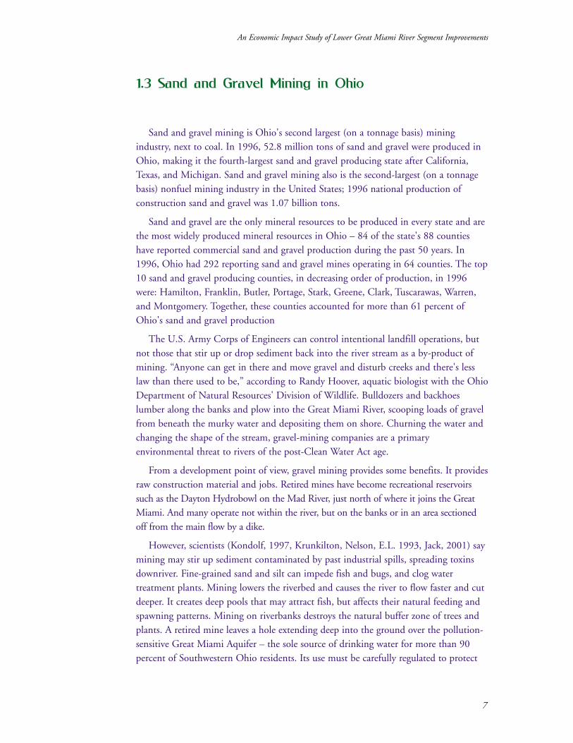
After mining, sand and gravel pits are among the least expensive mining sites to

reclaim and commonly are converted into aesthetically landscaped golf courses and

attractive building sites for new houses. Post-mining land values commonly exceed

pre-mining values when compared to non-mined land because of terrain improvements

and the creation of wetlands and lakes and ponds for boating, fishing, and swimming.

However, the appreciation of property values of most mining occurs only after

reclamation of the mines as parks and golf courses.

(http://www.ohiodnr.com/geosurvey/geo_fact/geo_f19.html)

9


Phot

o by

Mar

ilyn

Wal

l

1.4 Study Objectives

The objective of the study was to perform a comprehensive inventory of existing

economic conditions of the corridor such as property values, recreation and tourism

and estimate economic impacts of variations in water quality improvements and

infrastructure from selected improvements to the community thus providing a rationale

for investments in these improvements.

The study estimates through empirical analysis the effect of the following

improvements of river corridor attributes:

· Installation of a buffer strip/zone and a bike trail along the river

· Installation of more access points to the river

· Regulation of gravel mining, operation and reclamation on the banks

of the river

1.5. Methodology

Methodologies to estimate the impact of property, community and environmental

attributes on values of residential properties along the river, and the recreation and

tourism value of the river are the hedonic pricing (HP) method and the benefit transfer

(BT) method to determine the benefits and costs of buffer zones and new boating

access points. Types of gravel mining regulation and reclamation from other states are

summarized. HP and BT methods as well as information from interviewing local

people and gravel mining officials were used to get rough estimates of impacts.

Sustaining a River

10

Phot

o by

Mar

ilyn

Wal

l

11

Section 2

Estimating theEconomic Benefitsof Buffer Strips

Conservation is the foresighted

utilization, preservation and/or

renewal of forests, waters,

lands and minerals, for the

greatest good of the greatest

number for the longest time.

-Gifford Pinchot

Phot

o by

Mar

ilyn

Wal

l

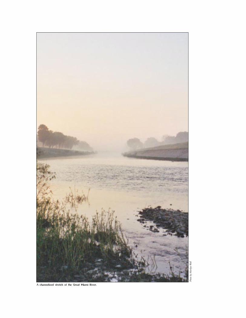
A channelized stretch of the Great Miami River.

2.1 Introduction

Within a watershed, generally the stream channel and adjacent land areas are

divided into three zones: aquatic, riparian, and upland. The aquatic zone includes the

stream and the area of the streambed that is normally underwater, i.e., the area below

the high water mark. The riparian zone lies between the aquatic and upland zone and is

an area of transitional vegetation influenced by its nearness to water. Riparian areas

sometimes include other types of wetlands and may have distinctive soil characteristics

(Helm 1985). Upland areas adjoin the riparian zone and are usually characterized by

vegetation and soils different from those in the riparian zone.

To protect aquatic and riparian resources, buffer strips are established in the riparian

zone directly beside the stream, and may extend to the adjacent upland zone. Buffer

strips are defined as strips of vegetation left beside a stream or lake after logging (Helm

1985). Buffer strips are also referred to as filter strips or protection strips. Appropriately

designed and managed buffer strips can contribute significantly to the maintenance of

aquatic and riparian habitat and the control of pollution.

Riparian buffer strips fulfill at least three basic roles. First, they help to maintain

the hydrologic, hydraulic, and ecological integrity of the stream channel and associated

soil and vegetation. For example, riparian vegetation helps maintain stream bank

stability and channel capacity. Riparian vegetation also contributes the large organic

debris (dead leaves, broken branches) that provides hydraulic structure to the channel.

Buffers trap fertilizers, pesticides, pathogens, and heavy metals, and they help trap snow

and cut down on blowing soil in areas with strong winds. In addition, they protect

livestock and wildlife from harsh weather and buildings from wind damage.

Second, buffer strips help protect aquatic and riparian plants and animals from

upland sources of pollution by trapping or filtering sediments, nutrients, and chemicals

from forestry and agricultural activities. Third, buffer strips protect fish and wildlife by

supplying food, cover, and thermal protection, and in some cases providing unique

habitat. An improved fish habitat also can improve fishery production, catch rates, and

recreational fishing opportunities. A 1998 study of the Great Lakes trout and salmon

fishery by Lupi and Hoehn suggests that a 10% increase in catch rates could lead to a

$3.4 million increase in recreational value for sport anglers. In addition, MacGregor

(1988) found that Ohio boaters would benefit $0.01 to $9.00 per one ton reduction in

sediment, and Bejranonda (1996) found that house values near Ohio lakes could

increase $0.04 to more than $25.00 per ton of sediment reduction.

13


Conservation buffers slow water runoff, trap sediment, and enhance infiltration within

the buffer. If properly installed and maintained, depending on width, they have the

capacity to:

· Remove up to 50 percent or more of nutrients and pesticides.

· Remove up to 60 percent or more of certain pathogens.

· Remove up to 75 percent or more of sediment.

(NRCS, 2001)

Conservation buffers work economically because of financial incentives available

through USDA conservation programs--the continuous Conservation Reserve Program

(CRP) sign-up, Environmental Quality Incentives Program (EQIP), Wildlife Habitat

Incentives Program (WHIP), general CRP, Wetlands Reserve Program (WRP), and

Stewardship Incentives Program (SIP).

Following are the financial incentives available through the continuous CRP sign-up:

· A signing incentive payment of $100 to $150 per acre for riparian

buffers, filter strips, grassed waterways, shelterbelts, field windbreaks,

and living snow fences.

· Up to 50 percent cost sharing for practice CRP installation.

· A practice incentive payment equal to 40 percent of eligible practice

CRP installation costs.

· A 20 percent rental rate (land rental) incentive for riparian buffers,

filter strips, grassed waterways, and field windbreaks.

· A 10 percent rental rate (land rental) incentive for wellhead

protection areas.

· Higher annual maintenance payments per acre for certain activities.

· Updated rental rates nationwide for installing riparian buffers on

marginal grazing land.

For farmers planning to participate in the program, no competitive offer is required

in the continuous CRP sign-up, and there is no waiting period. Offers are accepted

automatically if eligibility requirements are met, the land offered for enrollment is

suitable for the buffers landowners want to install, and they are willing to accept the

going rental rate, plus any incentives that might be offered.

Conservation buffers may help farmers meet Federal, state, or local pollution control

requirements. Many state and local governments, and some private organizations, offer

additional financial incentives to install conservation buffers.

Sustaining a River

14

2.2 Cost Effectiveness of Buffer Strips

Consistent with most analyses of the costs and benefits of natural resources

management alternatives, the costs of buffer strips are relatively easy to quantify, but the

benefits are not. Establishment of buffer strips normally results in additional costs to the

landowner, public or private. Costs incurred include the loss of stumpage, higher costs of

logging and road construction, and additional administrative costs (Streeby 1970).

Benefits from buffer strips accrue largely to the public and include improved bank

stability and water quality, enhanced fish and wildlife habitat, and greater aesthetic value.

Bollman (1984) noted that the costs of specific buffer strip prescriptions vary with

market conditions, the type of stand, and other variables, but were relatively easy to

evaluate. Conversely, benefits from the prescriptions were frequently non-market values-

-e.g., fish habitat, species diversity, and water quality – that were much more difficult to

evaluate. The question of equity arises when private land owners or logging firms must

bear the costs of operating in or around buffer strips that benefit sport fishermen, other

industries such as commercial fishing, or the general public (Gillick and Scott 1975).

The optimal width is by their definition the most cost-effective width. Considering

only the values of fish and logs, they found the "zero foot" buffer strip – i.e., no buffer

strip at all – to provide the greatest net economic value.

Based on studies in several tropical watersheds, this optimal buffer width was

estimated at 22 meters (73 feet) for perennial streams and less than 10 meters (33 feet)

for intermittent streams. This estimate, although not directly applicable to Ohio,

illustrates an alternative approach to evaluation of buffers based on financial criteria.

These studies suggest potential difficulties in establishing buffer strip areas or widths

based on economic criteria such as a benefit-cost ratio. First, as stated earlier, although

costs are relatively easy to determine, important non-market benefits are difficult to

evaluate. Second, the value society places on non-market riparian benefits such as

biological diversity is subject to not only measurement difficulties but also considerable

changes in public perception and relative scarcity, all of which are likely to be

substantially greater in the future.

Sohngen and Nakao (1999) tried to estimate the private benefits of filter strips for

Ohio farmers. In their fact sheet, two examples of revenue producing filter strips, hay

and timber, were developed. They estimated that for hay, the average price for alfalfa in

Ohio in 1996 was $134.58 per ton, and for other hay it was $75.42 per ton, using the

example of a mixture of Birdsfoot Trefoil and Kentucky Bluegrass planted with a no-till

system. Using a conservative price of $75 per ton, the annual returns for years 1 and 2

were $225, in years 3 and 4 they were $375, and in year 5 they were $338. The costs

of installing and maintaining filter strips on cropland include: (1) land rental costs, (2)

seed and fertilizer costs, and (3) equipment and labor costs.

15


As Table 2.1 indicates, all four options show net gains at 5 percent rate of interest,

but at 10 percent rate of interest, only grass and legume and hay are profitable. Hay

has a very high rate of return compared to all other options. In order for the farmers

to adopt these techniques, a widespread education program on the benefits of

filter/vegetative strips, along with the various options available to the landowners must

be launched.

The present study is confined to the two counties of Butler and Hamilton, and

data was collected accordingly. The parcel information of all land adjoining the banks

of the Great Miami River was collected, classified into categories of land use, such as

agricultural, residential, commercial, sand and gravel mining, land used for utilities such

as electric and telephone lines and railroads, government land used for state parks and

recreation, and land owned/acquired by the Miami Conservancy District for various

purposes such as flood control, wetland protection, construction of bike trails, etc.

In Butler County, on the west side of the river, agricultural land is mostly confined

to Madison and St. Clair Townships, and the rest of the land adjoining the river is

owned by the Miami Conservancy District, State of Ohio, Butler County Metro Parks

and other local government bodies. There are less than 30 residential parcels adjoining

the river on the east side of Butler County, and they are mostly concentrated in

Fairfield and Lemon Townships. The residential parcels are single-family dwellings, with

average parcel size less than half an acre. In such cases, to construct a buffer strip may

not be feasible, or cost effective for the landowner. Except for the few residential

parcels, the authors do not foresee any challenges in acquiring land for constructing

filter strips along the river. On the west side of the river, most residential property

adjoining the river is concentrated in Lemon, Hamilton, Fairfield and Madison

townships. Nearly 60% of the riverbank area is owned by several governmental

agencies, and the rest is owned privately.

As mentioned earlier in this section, it is assumed that farmers will voluntarily

participate in the continuous CRP sign-up program. Besides receiving the federal

incentives, the farmers will also benefit from the harvesting of hay from the filter strips.

It is to be noted here that only one third of the land adjoining the river is under

agriculture, and the remaining land is put under several other uses. A total of 52 miles

of riverbank length, (both sides of the river) is proposed to be brought under vegetative

Sustaining a River

16

Table 2.1Average Annual Profits (losses) From Alternative Filter Strip Options

(These values do not include land opportunity costs)

Types of Grass & Low HighVegetative Filter Strips Legume

HayTimber Timber

($ per acre per year)

Interest rate = 5%

Annual profits (losses) $4.81 $130.64 $10.57 $30.84

Interest rate = 10%

Annual profits (losses) $3.35 $122.82 ($5.77) ($9.92)

buffer strip in this study. The buffer strip would range between 33 feet and 75 feet,

depending on the nature of the river bank, the flow of the water, and the topology of

the land. The total area of the buffer strip would range between 208 and 384 acres.

In Hamilton County, out of the 321 parcels adjoining the river bank, 111, (roughly

one third) were residential properties, with 75 of these on the east side of the river and

36 on the west side. Therefore, the pattern of more residential properties on the east

side seems to be consistent in Hamilton County, too. Roughly 30 percent of the parcels

were agricultural land, and the rest were divided amongst industrial, commercial, gravel

and sand mining, government and other agency property and utilities and rail lines.

In order to estimate the dimensions of the filter strip, it is imperative to perform a

detailed analyses on the type of crops grown locally, collect considerable data on land

ownership and estimate the opportunity cost of land for each and every parcel owner

on the banks of the Great Miami River. Some of the owners of smaller parcels may

have a very high willingness to accept compensation for converting their present land

usage to vegetative filter strips. These analyses will take considerable time and resources,

which are not available to the authors at present time.

17


Phot

o by

Rob

San

der

s

Floodwalls such as this one along the Great Miami River can be rehabilitated with trees and light vegetation to make it more aesthetically pleasing to a community.

Phot

o by

Rob

San

der

sP

hot

o by

Mar

ilyn

Wal

l

This floodwall running by downtown Hamilton, Ohio could be rehabilitated to make it more aesthetically valuable to tourists and prospective homebuyers visiting the community.

A Great Blue Heron resting near the Troy Dam on the Great Miami River.

19

Section 3

Economic Analysisof the GreatMiami Bike Trail

Parks and reservations are

useful not only as fountains

of timber and irrigating rivers,

but as fountains of life.�

-John Muir

3.1 Introduction

In the present study, we are proposing a 28-mile bike trail starting at the Warren-

Montgomery County line, extending south to the confluence of the Great Miami River

and the Ohio River. The actual cost of the 28-mile bike trail would include land

acquisition costs, construction costs, and maintenance costs. For simplicity purposes, it

is assumed that there shall be no land acquisition costs, since most land in the proposed

bike trail site is owned by the MCD, or other governmental agencies, which have zero

opportunity cost for the land, as it is idle and not put to any economic use. The cost of

constructing a bike trail is estimated based on a Dubuque, Iowa Study as follows:

The cost of constructing a bikeway 28 miles long in 2000 was $2.9 million

approximately. The adjusted cost of the bikeway in the year 2003 is $3.2 million.

Maintenance cost, discounted present value, for 25 years (expected lifetime of the bike

trail) is $45,385. Total cost of the construction and maintenance of bike trail is about

$3 million.

This does not include the cost of purchasing rights-of-way and major bridge

structures. This estimate is based on current work for similar trails in other parts of

Ohio, as estimated by the Miami Conservancy District (MCD). It is anticipated that

about 75 percent of the cost will be paid by federal and state sources. The rest will be

shared among local public entities and private donors.

Most of the proposed right-of-way is on property owned by public agencies

including: the cities of Franklin, Middletown and Hamilton, as well as the Ohio

Department of Transportation, Metro Parks of Butler County and the Miami

Conservancy District. A small portion is privately held.

21


Table 3.1Cost of Non Motorized Multi Use Trails (Single Treadway)

Asphalt Surface, 10 Foot Width

Trail Unit Price Element Units Trail CostElement Per Unit Width Per Mile Per Mile

Clearing & Grubbing Acre $2000 14 feet 1.7 $3400

Grading Mile $3000 1 $3000

Granular Subbase Sq ft $0.40 12 feet 63360 $25,344

Asphalt Sq ft $1 10 ft 52,800 $52,800

Seeding/Mulching Acre $1 10 ft 0.5 $800

Other Costs 10% of trail cost $8,534

Contingency 15% of trail cost $122802

Total Cost per Mile $106,700

Maintenance Cost $ 5000/year

3.2 Benefit Transfer Results From Moore & Siderelis

The values used in the benefit transfer that follows were obtained from a 1995

study, published by Siderelis and Moore. The authors investigated net benefits of

bicycling and walking on abandoned railroad beds that have been converted to a

rail-trail for recreation purposes. A sample of three diverse rail-trails from across the

U.S., in Iowa, Florida and California were studied. Users were systematically surveyed

and counted on each trail during a period of one year, and were sent follow-up

mail surveys.

In the present study, we used the results from the Iowa bike trail, since it is the

closest match in demographic, trail landscape and income indicators to the Great

Miami Trail. The study findings state that on average, users spend $9.21 per day as a

result of their trail visit to the Heritage Trail in Iowa, $11.02 at St. Marks’ Trail in

Florida, and $3.87 per person per day at the Lafayette Trail in California. The findings

of the Iowa trail are applied in the present study, after inflating the $9.21 expenditure

to current dollars for the year 2003, using a consumer price index inflator.

The users are charged a fee of $1 per visit to the Iowa trail. Yearly visits to the trails

were about 135,000, 170,000, and 4,000,000 in the Iowa, Florida and California trails

respectively. Our study adopted the benefit cost method and applied the findings of

expenditures from the Iowa trail, and then applied the single point estimates of average

consumer surplus or willingness to pay (WTP) per activity day per person.

Sustaining a River

22

Table 3.2Benefits from the Great Miami Bike Trail

Estimate Lower Benefits Lower BenefitsBenefits by 25% by 50%

Calculated Yearly Visits to the Trail 135,000

Average Trip Expenditure

($ per person per day $11.09

adjusted to current dollars)

Total Annual Expenditures $1,497,150 $1,122,862 $748,575

Discounted Expenditures

in 25 years $11,285,938 $8,464,453 $5,642,969

Table 3.3Benefit Cost Ratio of Bike Trail

Benefits Benefit Cost Ratio4% Interest Rate 6% Interest Rate 8% Interest Rate 10% Interest Rate

Actual 7.21 5.90 4.92 4.19

Lower by 25 % 5.41 4.42 3.69 3.14

Lower by 50% 3.60 2.95 2.46 2.09

The second set of benefit transfer values used in this study are average consumer

surplus values per activity day per person from the study conducted by Siderelis and

Moore. Consumer surplus is a value of a recreation activity beyond what must be paid to

enjoy it. The benefit transfer estimate of a management, or a policy-induced change in

recreation is the average consumer surplus estimate for the average individual from the

benefit transfer literature. The mean, and the range of estimates for biking are

provided below:

Applying the mean of estimates to the usage, we obtain the recreational economic

benefits provided by the bike trail. Taking the lower bound estimate, the net benefits

are 2.8 million dollars, and taking the average for northeastern region, the net benefits

are about 5.7 million dollars, per year.

23


Phot

o by

Rob

San

der

s

This concrete channelway along the Great Miami River in Hamilton, Ohio, could be refurbished with shade trees to accommodate a bike trail and to enhance and beautify the downtown area.

Table 3.4Average Consumer Surplus Values Per Activity Day Per Person

Activity Biking Adjusted to Year 2003

Mean of Estimates $ 45.15 $54.36

Lower Bound $17.61 $ 21.20

Upper Bound $62.68 $75.71

Mean for Northeast Region $34.11 $42.27

Total number of visitors/users: 135000

Total Economic Benefits (lower bound): 135000 x $21.20 = $2,863,350. ($2.8 million)

Total Average Economic Benefits (mean for northeast): 135000 x $42.27 = $5,706,450. ($5.7 million)

Phot

o by

Mar

ilyn

Wal

lP

hot

o by

Mar

ilyn

Wal

l

The Taylorsville Dam above Dayton was designed by Arthur Morgan as a Dry Dam to help with flood prevention.

25

Section 4

Economic Impact of Gravel Mining

If future generations are to

remember us with gratitude

rather than contempt, we

must leave them more than

the miracles of technology.

-President Lyndon B. Johnson

Phot

o by

Rob

San

der

sP

hot

o by

Rob

San

der

s

Welch Sand & Gravel mining operation.

Dravo Park mining operation.

4.1 Introduction

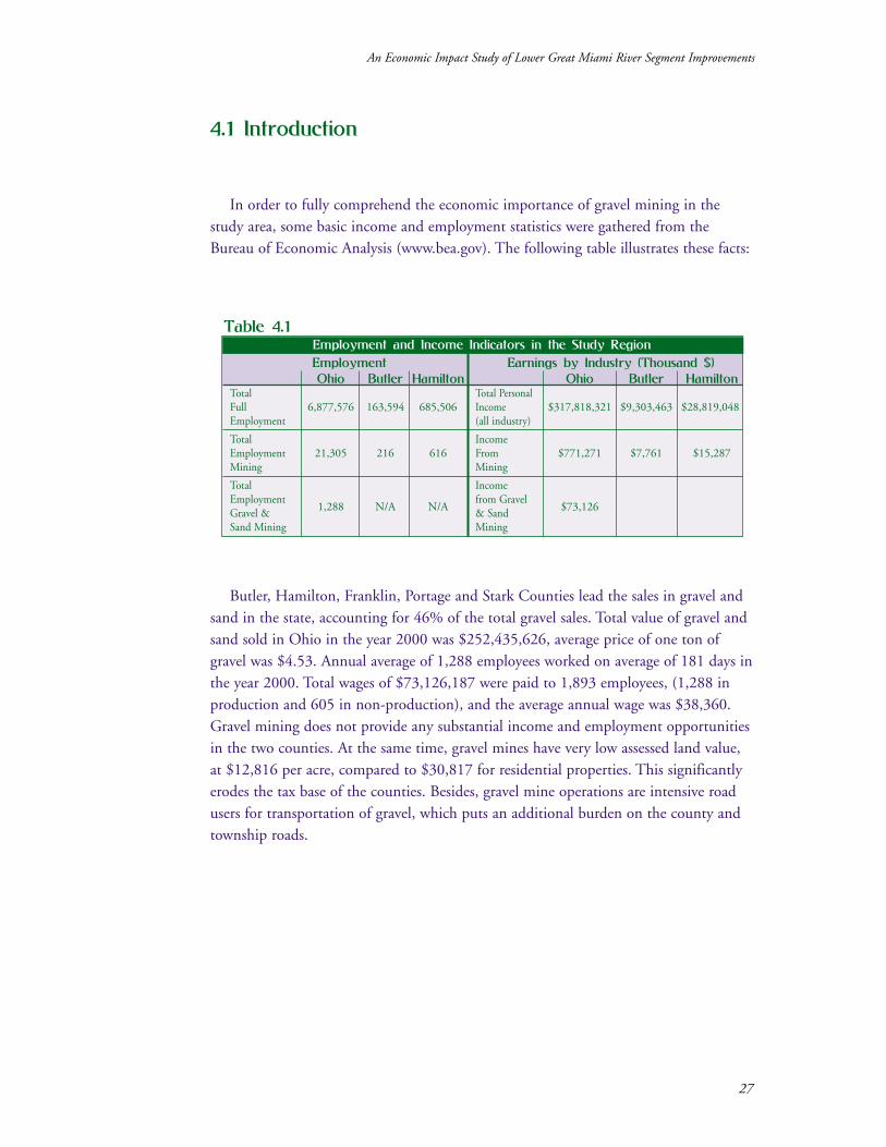
In order to fully comprehend the economic importance of gravel mining in the

study area, some basic income and employment statistics were gathered from the

Bureau of Economic Analysis (www.bea.gov). The following table illustrates these facts:

Butler, Hamilton, Franklin, Portage and Stark Counties lead the sales in gravel and

sand in the state, accounting for 46% of the total gravel sales. Total value of gravel and

sand sold in Ohio in the year 2000 was $252,435,626, average price of one ton of

gravel was $4.53. Annual average of 1,288 employees worked on average of 181 days in

the year 2000. Total wages of $73,126,187 were paid to 1,893 employees, (1,288 in

production and 605 in non-production), and the average annual wage was $38,360.

Gravel mining does not provide any substantial income and employment opportunities

in the two counties. At the same time, gravel mines have very low assessed land value,

at $12,816 per acre, compared to $30,817 for residential properties. This significantly

erodes the tax base of the counties. Besides, gravel mine operations are intensive road

users for transportation of gravel, which puts an additional burden on the county and

township roads.

27


Table 4.1Employment and Income Indicators in the Study Region

EmploymentOhio Butler Hamilton

Total

Full 6,877,576 163,594 685,506

Employment

Total

Employment 21,305 216 616

Mining

Total

Employment

Gravel &1,288 N/A N/A

Sand Mining

Earnings by Industry (Thousand $)Ohio Butler Hamilton

Total Personal

Income $317,818,321 $9,303,463 $28,819,048

(all industry)

Income

From $771,271 $7,761 $15,287

Mining

Income

from Gravel

& Sand$73,126

Mining

4.2 Hedonic Pricing Method

Hedonic pricing analysis begins by measuring the price differentials that arise

due to quality differences across similar goods. Hedonic pricing uses the different

characteristics of a traded good to estimate the value of a non-traded good. For

example, the value of a piece of riverfront could be calculated by comparing the price

of a house on the riverfront with the price of a similar house located elsewhere.

By correcting and/or controlling for other factors that would influence the value of

a particular property, economists are able to isolate the implicit price of some amenity

or bundle of amenities, in this example riverfront property that has changed over time.

The price of a house may be affected by physical/structural characteristics such as

number of bedrooms, finished living area, number of bathrooms; neighborhood

characteristics such as proximity to schools, zoning/subdivision regulations, and

proximity to, or quality of environmental attributes such as existence of a large egg

farm, golf course, state scenic river, etc. Hedonic methods can be used to estimate

effects of certain disamenities on the price of a residential property; for example, the

price of a property adjacent to an area affected by industrial pollution, or proposed

undesirable developments such as a large airport.

The process of estimating a hedonic pricing function relating housing pricing to

quantities of various characteristics of a residential property is relatively straightforward

and based on a regression model. However, to derive aggregate value measures from

these estimated functions is more complicated, and a two-stage regression equation is

required in most cases, particularly if the changes in characteristics are relatively large.

The hedonic technique depends on observable data from actual behavior of

individuals. Market data on property sales and characteristics are available through local

government sources such as county auditor’s offices and can be used in conjunction with

secondary data. However, many environmental amenities have only small, if any effects

on housing prices, and may be difficult to estimate using econometric methods. Besides,

many factors that influence the housing property value may be correlated, for example,

local schools may not be as good in a poorer community, and the community may be

located near an environmental disamenity, such as a dump or slaughter house.

Sustaining a River

28

4.3 Data Collection

The river flows through six Counties: Logan, Shelby, Miami, Montgomery, Butler

and Hamilton. The first three were not included since gravel mining is not a serious

issue there. Butler and Hamilton counties are comparable respecting gravel mining.

Data were gathered regarding property parcels located in the townships along the river.

There are 119 homes in the sample. This is approximately 25 percent of the population

of homes. The townships not adjoining the river were dropped from the sample, since

the main objective of this section of the study was to determine the effect of river gravel

mining on property values. The value of the homes was recorded from the county

auditors’ offices. This is the market-assessed value of the property. The values for the

year 2002 were taken for the study.

Information on the structural characteristics was also available from the parcel cards

from the auditors’ offices. Data for other characteristics, such as distance to gravel

mines, distance from the urban centers, were obtained from the maps from the County

Engineers’ offices.

The final hedonic price function for the model is expressed as:LnVal = _ + _1Eastside + _2Distance to Gravel Mine + _3Distance to Urban Center + _4Ln Acres + _5Downstream + _6LnAge + _7StoryHeight + _8Rooms + _9Bedrooms + _10Living Area + _11AirCondition + _12Heating + _13Fireplace + _14Half Bath + _15Full Bath

Structural characteristics of a house are described by: number of rooms, number of

bathrooms, garage spaces, age, various utilities including water supply, sewer system,

septic system and electricity. Other things equal, we expect that an additional bedroom

or bathroom represent an extra amenity. The lifespan or durability of a house is

associated with age and or type of construction. Since a majority of the houses were of

29


Table 4.2Hedonic Model Coefficient Estimates (A=accept, R=reject)

Parameter VariableEstimate

t Value 20% 10% 5% 2%

Intercept 12.7 7.73 A A A A

East Side -0.13 -0.71 R R R R

Distance to Gravel Mine 167.26 13.53 A A A A

Distance to Urban Center -23.38 -4.87 A A A A

Acreage (lot size) 0.34 6.02 A A A A

Downstream 0.01 0.08 R R R R

Age -0.22 -1.58 A R R R

Story Height -0.29 -1.21 R R R R

Number of Rooms -0.15 -1.73 A A R R

Number of Bedrooms 0.18 1.33 A R R R

Living Area 0.05 0.18 R R R R

Air Conditioning 0.23 1.07 R R R R

Heating -0.22 -0.67 R R R R

Fireplace 0.59 2.74 A A A A

Half Bath 0.64 1.87 A A R R

Full Bath 0.09 0.44 R R R R

the same type of construction, we did not include this variable. In light of the historical

significance of houses more than a century old, we attempted to define age as a non-

linear (inverse) variable in the model. Since the results were not conclusive, a log form

was adopted. Distance to the three urban centers is intended to provide a measure of

relative locational advantage. The functional form that performed the best was a log-

linear mixed form. The assessed value of property (the dependent variable), total

acreage of the parcel, total living area, and age of the house were specified in log form.

Log-linear mixed form incorporates diminishing marginal utility. A linear model would

not have been desirable because it assumes that implicit price is constant regardless of

the quantity of the attribute.

The model explains 49% (adjusted R2) of the variation in the data. Eight of the 15

estimated coefficients are significantly different from zero at the 20%, six at 10%

significance and four at 5% significance level respectively, as illustrated in Table 4.2.

The coefficients for living area, acreage and age are elasticities, interpreted as percentage

change in the value of a property due to a 1% change in the quantity of that

characteristic, other things remaining the same. The other coefficients that represent

change in the price due to a unit changes in the respective variables. As the area of the

property increases by one percent, the value of the property is expected to increase by

approximately 0.35 percent. Similarly, as the total living area increases by one percent,

the value of the property is expected to increase by 0.048 percent. As the age of the

house increases by one year, the value of the house is expected to decrease by 0.22

percent. The value of the property is expected to decrease by $131 if the property is

located on the east side of the river, an additional room will decrease value by $150, an

additional bedroom will increase the value by $180, and an additional bathroom by

$90 and an additional half bath by $640.

As an average, as distance to the gravel mine increases by one mile, the value of the

property increases by $16,725. The assessed market values of the residential properties

were expressed in thousands of dollars, and the coefficient, 167.25 is multiplied by

1000 to get the scale specific coefficient. It is assumed that the impact is insignificant

beyond the one mile limit.

Total number of single family dwellings = 238

Total number of houses in the corridor within one mile of a gravel mine = 172

Total loss of residential property value proximity (one mile or less) due to gravel mines = 172 x 16,725 = $2,876,700 (2.8 million, approx)

The total decrease of revenues annually to the local government due to decreased

property value resulting from proximity to gravel mining is estimated at $119,153.

Sustaining a River

30

Table 4.3Tax Revenue Implications of Gravel Mining

County Tax Coefficient Number of Houses Tax Revenue ($)Millage Est in the Area

Butler 41.37 16725 64 (41.37 x 16725 x 64)/1000 = 44282.5

Hamilton 41.45 16725 108 (41.45 x 16725 x 108)/1000 = 74871.1

Total 119,153

4.4 Regulation of Sand and Gravel Mining

In-stream mineral mining is prohibited in many countries including England,

Germany, France, the Netherlands, and Switzerland, and is strongly regulated in

selected rivers in Italy, Portugal, and New Zealand (Kondolf 1997, 1998). In the

United States, in-stream mining may be the least regulated of all mining activities

(Waters 1995; Starnes and Gasper 1996) and regulations vary by state. In Ohio,

Governor Bob Taft signed Senate Bill 83, in December 2001; effective March 15, 2002

giving inspectors with the Ohio Department of Natural Resources (ODNR) increased

oversight of the mining of industrial minerals such as limestone, gravel and clay. Before

the passing of the bill, few restrictions governed mineral mining instream channels and

floodplains; counties and municipalities operated largely unregulated. Some instream

mining operations do not have the necessary permits, and permitting agencies are

under funded for their function of tracking compliance (Fairchild et al. 1997).

ODNR Director Sam Speck said the legislation (Senate Bill 83) represents the first

comprehensive overhaul of the state's industrial minerals law since 1974. According to

Speck, “This law significantly strengthens our ability to protect groundwater supplies

through increased regulation of in-stream and near-stream mining. It also provides local

communities with a stronger voice in decision making as to the location of proposed

mines or quarries… And this legislation has considerable support from the mining

industry as it brings the regulatory process up to date and makes it more efficient and

timely.” (For details, see Fiscal Note & Local Impact Statement 124th General

Assembly of Ohio, Ohio Legislative Service Commission Internet Web Site:

http://www.lsc.state.oh.us)

31


Phot

o by

Rob

San

der

s

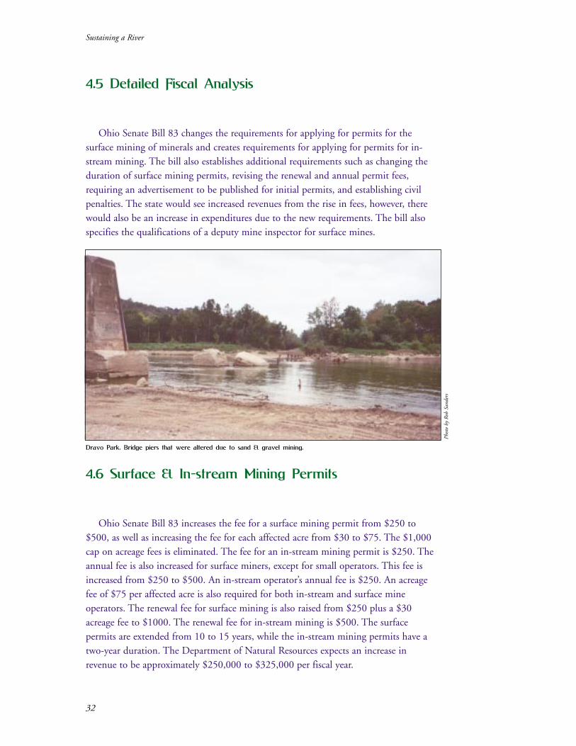
4.5 Detailed Fiscal Analysis

Ohio Senate Bill 83 changes the requirements for applying for permits for the

surface mining of minerals and creates requirements for applying for permits for in-

stream mining. The bill also establishes additional requirements such as changing the

duration of surface mining permits, revising the renewal and annual permit fees,

requiring an advertisement to be published for initial permits, and establishing civil

penalties. The state would see increased revenues from the rise in fees, however, there

would also be an increase in expenditures due to the new requirements. The bill also

specifies the qualifications of a deputy mine inspector for surface mines.

4.6 Surface & In-stream Mining Permits

Ohio Senate Bill 83 increases the fee for a surface mining permit from $250 to

$500, as well as increasing the fee for each affected acre from $30 to $75. The $1,000

cap on acreage fees is eliminated. The fee for an in-stream mining permit is $250. The

annual fee is also increased for surface miners, except for small operators. This fee is

increased from $250 to $500. An in-stream operator’s annual fee is $250. An acreage

fee of $75 per affected acre is also required for both in-stream and surface mine

operators. The renewal fee for surface mining is also raised from $250 plus a $30

acreage fee to $1000. The renewal fee for in-stream mining is $500. The surface

permits are extended from 10 to 15 years, while the in-stream mining permits have a

two-year duration. The Department of Natural Resources expects an increase in

revenue to be approximately $250,000 to $325,000 per fiscal year.

Sustaining a River

32

Phot

o by

Rob

San

der

sDravo Park. Bridge piers that were altered due to sand & gravel mining.

4.7 Surface & In-stream Mining Administration

Provisions in the bill require the OhioDepartment of Natural Resources to make

significant improvements to existing practices dealing with surface mining. The

department already does some provisions within the bill such as upgrading blasting

standards and certification. There are also additional requirements such as groundwater

modeling. The department will also have to implement procedures dealing with in-

stream mining. The department does not currently regulate in-stream mining in Ohio.

It is currently only regulated by the Army Corps of Engineers. The department

estimates that 3 to 6 employees will be needed due to the addition of groundwater

modeling requirements, additional permit reviews, enhanced inspection, and added

bonding administration costs. These positions will deal with the following: hydrology,

application manager, blasting specialist, and inspectors. Overall, the department

estimates that the costs to implement this bill will be between $750,000 to $900,000.

The increased revenues from surface mining fees will offset a portion of this cost.

The bill also calls for phased reclamation, which is applied to both in-stream and

surface mining. This allows the mining operator to file a request for inspection of land

that has completed a phase of reclamation. After inspection from each phase, the Chief

must issue an order to the operator and the operator’s surety releasing them from

liability on an applicable amount based on the reclamation completed. This may lead to

more reclamation inspectors, which will be a minimal increase in expenditures.

The Ohio Senate Bill 83 requires an advertisement to be published before an initial

permit is issued. It is also required for a renewal permit and any amendments that

significantly affect a permit. The bill allows written comments and objections to the

issuance of a permit. The bill also establishes civil penalties and provides for civil

actions for the relief of violations to the Surface Mining Law. There are approximately

50 violations annually of the Surface Mining Law. These cases are generally resolved

before any court proceedings are necessary. There are expected to be no fiscal effects on

political subdivisions due to these provisions.

33


Phot

o by

Rob

San

der

s

Welch Sand & Gravel mining operation.

35

Section 5

Economic Analysisof ProposedAccess Points

Wilderness areas are first

of all a series of sanctuaries

for the primitive arts of

wilderness travel, especially

canoeing and packing.

-Aldo Leopold

Phot

o by

Mar

ilyn

Wal

lP

hot

o by

Mar

ilyn

Wal

l

5.1 Introduction

In order for local and state governments to allocate funds efficiently in recreational

waterway activities, they need to know how beneficial these activities are likely to be.

Recreational boating for example has been identified to provide not only a significant

economic impact but also a wide range of social and psychological benefits. As a result,

expanding boating opportunities by constructing new boat ramps where needed is

expected to not only enhance the recreational options of a given region but also to

boost the local economy. In this perspective, the Great Miami River remains a potential

valuable natural asset for the counties it flows through. The economic potential of the

river is due to the scenic beauty of its corridor and the quality of its water. The Great

Miami River water quality is far better than the average river in Ohio. According to the

National Park Service, this part of the river is qualified to be a National Wild and

Scenic River. However, because access points are lacking, the river is inconvenient for

most recreational users, making it a greatly undervalued and underused natural

resource. Such underutilization creates rationale for improving the Great Miami River

segments by increasing the number of access points. We define an access point as any

area that borders the river and may be accessible by car. An access point could be

positive, such as a bike path, park, or boat launch; or negative, a place used for illegal

dumping; or potentially positive, an area that could be developed for community

recreational use.

The purpose of this section is to determine the benefits and costs from the

allocation of funds to construction of new access points in Butler and Hamilton

counties, Ohio through an ex-anti analysis of the potential behavior of Great Miami

River users. An attempt to identify the benefits is the first step in valuing them. The

potential benefits of improving the Great Miami River can be summarized as follows:

· Increase in recreational opportunities

· Increase in real estate value such as land and housing

· Increase in employment in the production and service sectors

· Tourism development

· Increase in the government tax base

· Increase in the surrounding population welfare

The costs to bring these benefits into existence include building the new access

points, making them operational, and maintaining them. Methodologically, it would be

ideal to use survey-based methods such as contingent valuation or contingent choice.

However, these methods would generally be expensive and more difficult to apply given

the time and funds allotted for the study. Alternatively, the benefit transfer method

appears to be more appropriate because it allows the researcher to obtain economic

estimates for a particular study using secondary data and previous studies at other sites.

37


In applying the benefit transfer method the first step is to identify existing studies

or values that can be used for the transfer. The second step is to determine based on

relevant criteria whether these values are transferable. The next step is to assess the

reliability of the previous studies. Finally, using available and relevant information, the

existing values need to be adjusted to better mirror the values for the policy site

(Desvouges et al. (1992).

To the best of our knowledge, in the literature, there is no particular study that

looked at how river users would change their behavior if new river access points were to

be brought into existence. In order to quantify the benefits resulting from additional

access points, the following data are required:

· Total number of users, and increase in users, particularly boaters due to

installation of access points,

· Average amount spent per user per trip to the river.

The analysis adopts two studies, authored by Hitzhusen et al. (2000), and Silva et al., for

benefit transfer. Hitzhusen et al. estimated the number of users and estimated benefits

accruing from river use in the Muskingum River. Silva et al. (1997) analyzed the behavior of

Ohio boaters at newly constructed ramps on Ohio rivers and lakes using a survey-based

method. As a result, these studies provide a good basis for benefit transfer. As well

established in the literature on the benefit transfer approach, using these figures for transfers

requires their adaptation to the policy site characteristics (Rosenberger and Loomis, 2000).

The lack of information on the Great Miami River policy site has motivated the need to

collect some baseline data. The method used is similar to the Delphi technique in the sense

that it involves collecting opinions of a group of 10 people knowledgeable about the river

use (see Appendix I at end of this document for details). As the Delphi method is

contingent upon the judgment of knowledgeable experts (Martino, 1970), the results of the

survey rely heavily on the opinion and information released by the respondents.

The questionnaires contained two types of questions. The first set of questions

address the respondents’ own use of the river and the second set asks for the respondents’

opinion about how other people use the river. The questions concern types of use,

frequency of use, trip supplies, expenditure on trips, additional visitation in response to

potential installation of new access points to the river, and inhibiting factors to increased

use. Based on the survey results and findings by other studies, new estimates are

calculated. It is noteworthy that the outcomes of this survey do not establish strong and

generalizable statistical evidence, they just report opinions of a small group of

knowledgeable users of the river, and should be considered and interpreted as such.

This study is not the first to aim at estimating recreation demand when user counts

are unknown even if the number of visits is estimated by adding gate counts, tickets, or

direct observations. A study by Johnston and Tyrrell (in AJAE August 2003)

highlighted the problems inherent in lack of information on user counts and proposed

an estimation method. However, since it is based on the known total number of visits,

their method is not applicable here.

Sustaining a River

38

5.2 Types of Use of the River

Questionnaire respondents were asked to indicate their primary activity when taking

trips to the river. Most of them point out that they use the river mostly for

walking/jogging, boating, fishing and wildlife viewing. When asked about what they see

other people use the river for, almost all respondents point to walking/jogging and fishing.

The respondents were also asked how often they use the river in a month during the

Spring to Fall season. The answers vary according to whether the respondents live

close to or far from the river or depending on whether they have easy or difficult

access. Those who live close indicate that their use of the river ranges from 8-10 times

to 12-15 times in a month, whereas those having limited access report to have used

the river between 1-2 times to 3-5 times. Combining all respondents, the number of

trips taken to the river averages five trips in a month. Since any outdoor activity is

weather or temperature driven, these trips are typically taken from Spring to Fall with

the peak use time in Summer. For hunters, the peak use time would coincide with the

duck/goose season.

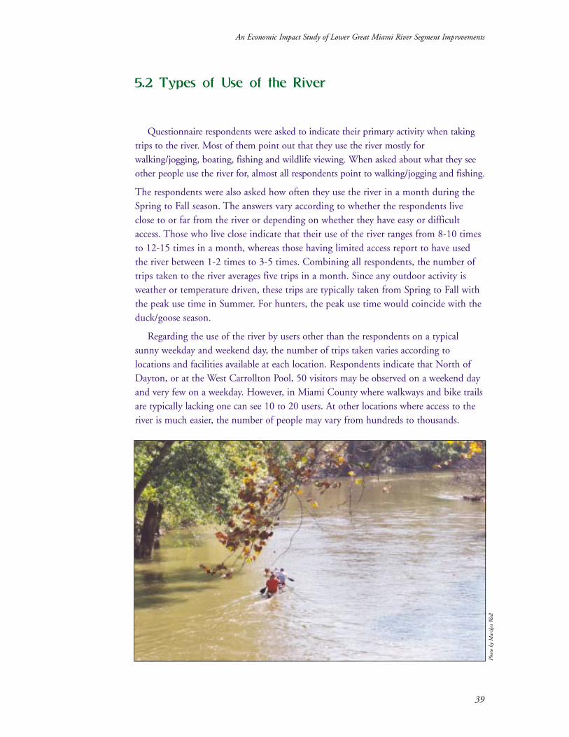
Regarding the use of the river by users other than the respondents on a typical

sunny weekday and weekend day, the number of trips taken varies according to

locations and facilities available at each location. Respondents indicate that North of

Dayton, or at the West Carrollton Pool, 50 visitors may be observed on a weekend day

and very few on a weekday. However, in Miami County where walkways and bike trails

are typically lacking one can see 10 to 20 users. At other locations where access to the

river is much easier, the number of people may vary from hundreds to thousands.

39


Phot

o by

Mar

ilyn

Wal

l

5.3 Trip Expenses

A specific question asks the respondents to estimate the amount of money they

spend on average when taking trips to the river. Since most of them live close to the

river, their trip costs appear to be relatively small compared to results of other studies.

However, almost everyone has reported expenditures on food, gas and fishing supplies.

Those whose trip purpose is hunting as well as fishing spend some money on fishing

and hunting licenses. The amount of money reported spent on purchases for a trip

varies between 5 and 10 dollars. This figure, however, does not include canoe and boat

rentals, which makes the estimate a low-bound estimate.

Sustaining a River

40

Phot

o by

Mar

ilyn

Wal

l

5.4 Increase in River Use

To address the issue of additional trips to the river due to an improvement in access,

respondents were asked to indicate whether they and other users would increase their

visitation if more access points become available. If the answer is affirmative, they were

asked by how much they would be willing to increase their use. As expected, those who

have easy and close access to the river argue that they would be less likely to increase

their use. Whereas, those who live further from the river and who have very limited

access report that they would double their use if more access points become available.

They seem to be relatively knowledgeable about the current access conditions of the

river. They state that access to the river is a major problem specifically when it comes to

fishing from canoes. Increasing trips of course depends on the type of access points

provided and the need for each type at specific locations. For some respondents, road

and parking access would imply increase in use. For others, an increase in ramps for

small boats would enhance boating traffic. Apparently, given the current access

conditions, provision of access points should primarily target two areas: fishing (access

for small boats) and walkway and bike trail. Although the respondents were cautious in

making an educated guess about additional use by other users, they all agreed that new

access points mean new places, more variety and more choices. Consequently, if they

are made available, people will use them, as they will make access easier. In addition,

the respondents were invited to identify some inhibiting factors that would restrain

them from increasing their use even if more public access points are provided. Among

others, poor aquatic habitat was mostly mentioned.

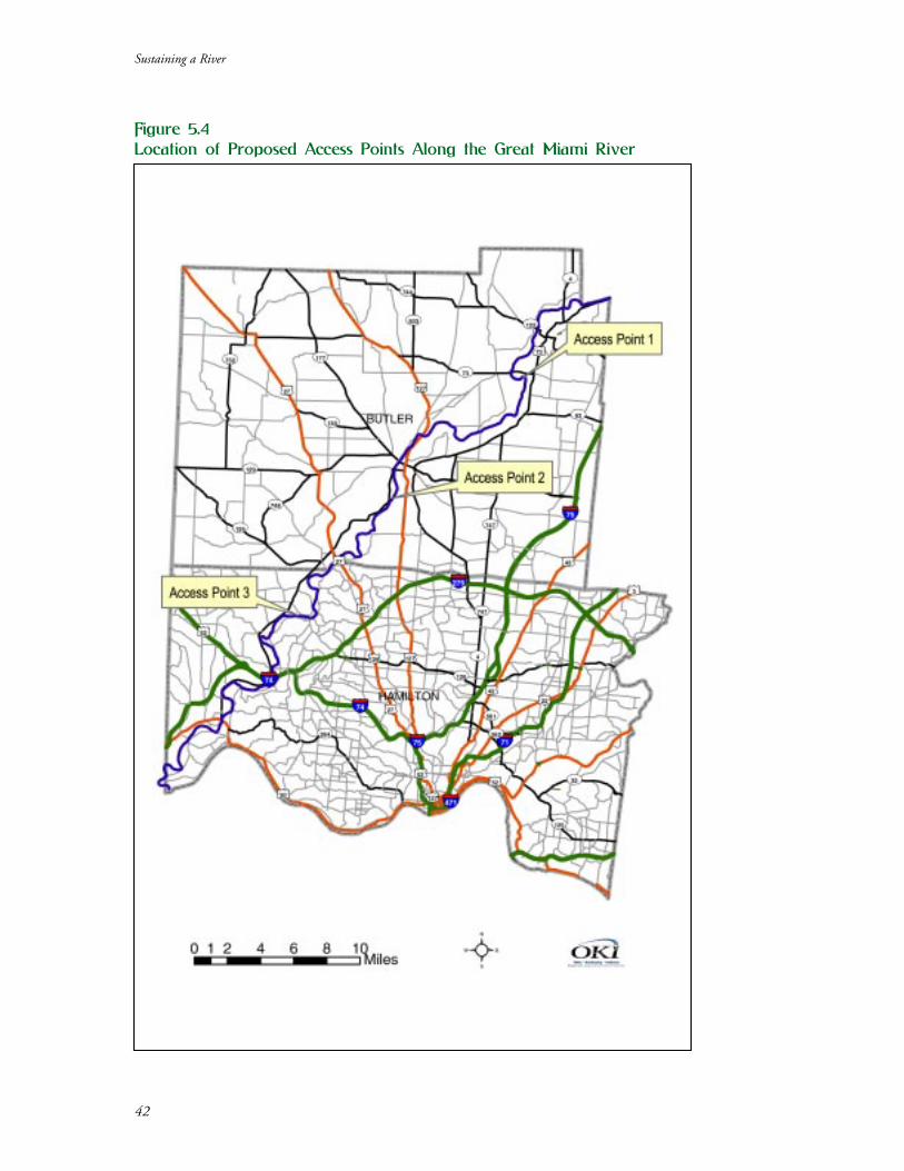
For installing the access points, three locations were identified based on distance to

major artery/road, distance to food and water facilities, proposed bike path locations,

distance to current access points and distance to clusters of gravel mines. We suggest

placing two access points in Butler County and one in Hamilton County. Access point

1 would be located in the Burnet Woods park and recreation area, on the East side of

the river along Middletown Road. Access point 2 would be installed nearby Avon

Woods outdoor Education Center, on the east side of the river, along Neilan Boulevard.

Finally, access point 3 would be placed on the west side of the river near Haven Road

(See Figure 5.4 on the following page for location of the proposed access points).

41


Sustaining a River

42

Figure 5.4Location of Proposed Access Points Along the Great Miami River

43


5.5 Estimated Benefits of Proposed Access Points

The purpose of conducting the survey was to adjust the estimated benefits calculated

from an earlier study of the total visitation to the Muskingum River. It is evident from

the survey results that visitation to the river is related to whether the respondents live

distant from or close to the river. The total visitation reported averages five trips a

month, implying an average use of about one time a week. The relative dependence of

this outcome on the location of the respondents’ residence calls for a conservative but

reasonable assumption that people take trips to the river two times during two

weekends in a month and devote the other 2 weekends to other activities. Based on the

idea that outdoor recreation is seasonal, there is a need to account for seasonality

effects. Consequently, annual average visitation per user is assumed to be 18 (2x9) trips.

Relying on the Delphi survey respondents for the total visitation estimate would be

inappropriate since this estimate would not result from a truly random sample.

Alternatively, the study by Hitzhusen et al. (2000) on the Muskingum River is used for

benefit transfer. In this study, data on the annual river use were collected on a daily

basis by lockmasters at each lock and maintained by Blue Rock State Park in

Muskingum County. Between 1983 and 1997, total visitation to ten locks and dams

averages 190,000 annually. Although the population living in Butler and Hamilton

counties is almost twice the population of the counties comprising the Muskingum

River watershed, half of this number, i.e., 95,000 visits is used as a conservative

assumption. This is because the Muskingum River has more access points.

In order to estimate additional spending by river users assuming availability of new

access points, we need to estimate increase in visitation to the river. The results of the

survey are very informative but not sufficient to precisely estimate the increase in

visitation, creating the motivation for applying benefit transfer. Instead of using four

additional visits a year as reported by Silva et al. (2000), a conservative amount of three

visits is used. However, to value visitation to the river, the conservative $10 from the

Delphi survey is used as average expenditure per user and per trip, which is reasonable as

compared to estimates of $13.50 for the Northeast region (Region 9) provided by the

U.S. Forest Service. Increase in visitation is determined by drawing upon findings by

Sylva et al. (2000) that 26.1% of users would increase their use by three visitation days if

more access points were installed.

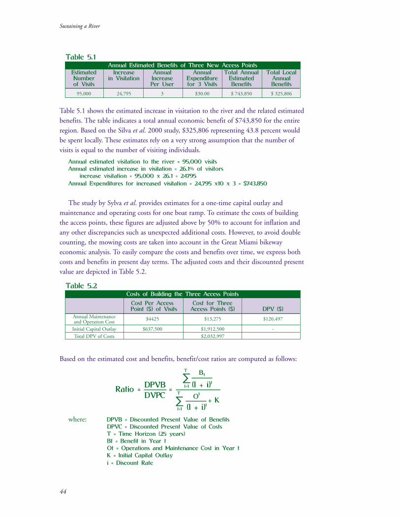
Sustaining a River

44

Table 5.1 shows the estimated increase in visitation to the river and the related estimated

benefits. The table indicates a total annual economic benefit of $743,850 for the entire

region. Based on the Silva et al. 2000 study, $325,806 representing 43.8 percent would

be spent locally. These estimates rely on a very strong assumption that the number of

visits is equal to the number of visiting individuals.

Annual estimated visitation to the river = 95,000 visitsAnnual estimated increase in visitation = 26.1% of visitors

increase visitation = 95,000 x 26.1 = 24795

Annual Expenditures for increased visitation = 24,795 x10 x 3 = $743,850

The study by Sylva et al. provides estimates for a one-time capital outlay and

maintenance and operating costs for one boat ramp. To estimate the costs of building

the access points, these figures are adjusted above by 50% to account for inflation and

any other discrepancies such as unexpected additional costs. However, to avoid double

counting, the mowing costs are taken into account in the Great Miami bikeway

economic analysis. To easily compare the costs and benefits over time, we express both

costs and benefits in present day terms. The adjusted costs and their discounted present

value are depicted in Table 5.2.

Based on the estimated cost and benefits, benefit/cost ratios are computed as follows:

where: DPVB = Discounted Present Value of BenefitsDPVC = Discounted Present Value of CostsT = Time Horizon (25 years)Bt = Benefit in Year tOt = Operations and Maintenance Cost in Year tK = Initial Capital Outlay

i = Discount Rate

Table 5.1Annual Estimated Benefits of Three New Access Points

Estimated Increase Annual Annual Total Annual Total LocalNumber in Visitation Increase Expenditure Estimated Annualof Visits Per User for 3 Visits Benefits Benefits

95,000 24,795 3 $30.00 $ 743,850 $ 325,806

Table 5.2Costs of Building the Three Access Points

Cost Per Access Cost for ThreePoint ($) of Visits Access Points ($) DPV ($)

Annual Maintenance and Operation Cost

$4425 $13,275 $120,497

Initial Capital Outlay $637,500 $1,912,500 -

Total DPV of Costs $2,032,997

Ratio = =DPVB

DVPC

t=1

T

t=1

T

(l + i)t

(l + i)tBt

Ot

+ K

∑

∑

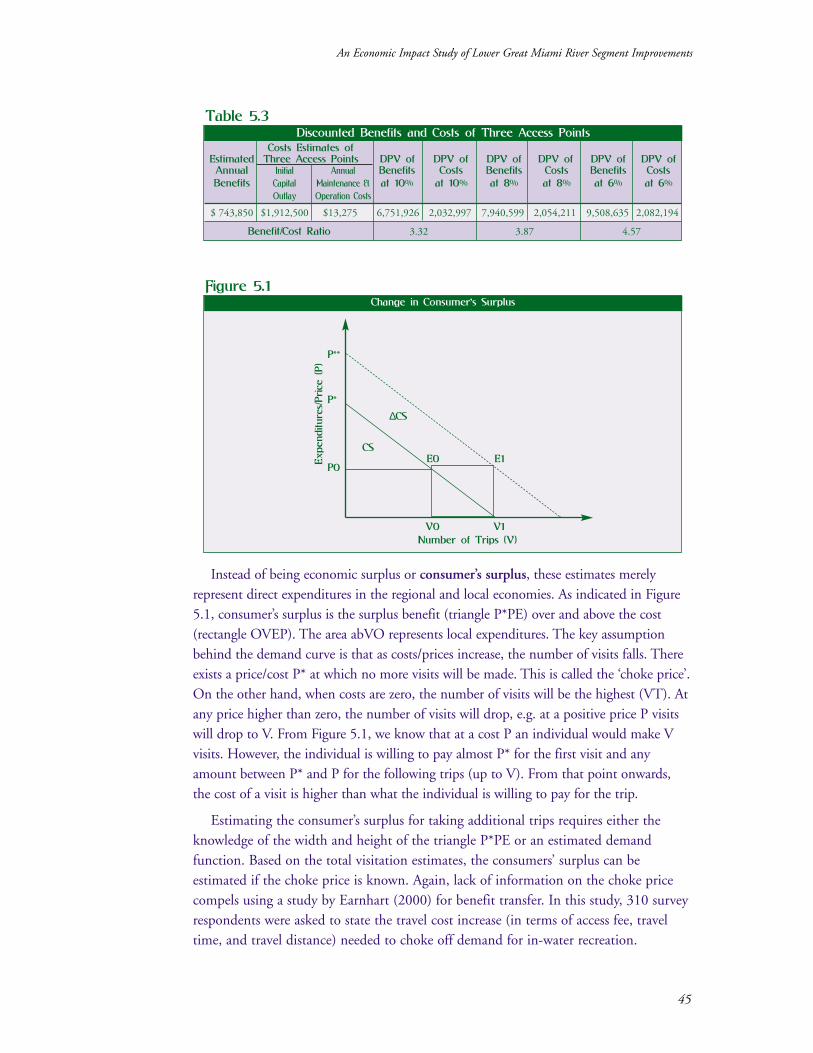
45


Instead of being economic surplus or consumer’s surplus, these estimates merely

represent direct expenditures in the regional and local economies. As indicated in Figure

5.1, consumer’s surplus is the surplus benefit (triangle P*PE) over and above the cost

(rectangle OVEP). The area abVO represents local expenditures. The key assumption

behind the demand curve is that as costs/prices increase, the number of visits falls. There

exists a price/cost P* at which no more visits will be made. This is called the ‘choke price’.

On the other hand, when costs are zero, the number of visits will be the highest (VT). At

any price higher than zero, the number of visits will drop, e.g. at a positive price P visits

will drop to V. From Figure 5.1, we know that at a cost P an individual would make V

visits. However, the individual is willing to pay almost P* for the first visit and any

amount between P* and P for the following trips (up to V). From that point onwards,

the cost of a visit is higher than what the individual is willing to pay for the trip.

Estimating the consumer’s surplus for taking additional trips requires either the

knowledge of the width and height of the triangle P*PE or an estimated demand

function. Based on the total visitation estimates, the consumers’ surplus can be

estimated if the choke price is known. Again, lack of information on the choke price

compels using a study by Earnhart (2000) for benefit transfer. In this study, 310 survey

respondents were asked to state the travel cost increase (in terms of access fee, travel

time, and travel distance) needed to choke off demand for in-water recreation.

Table 5.3Discounted Benefits and Costs of Three Access Points

Costs Estimates ofEstimated Three Access Points DPV of DPV of DPV of DPV of DPV of DPV ofAnnual Initial Annual Benefits Costs Benefits Costs Benefits CostsBenefits Capital Maintenance & at 10% at 10% at 8% at 8% at 6% at 6%

Outlay Operation Costs

$ 743,850 $1,912,500 $13,275 6,751,926 2,032,997 7,940,599 2,054,211 9,508,635 2,082,194

Benefit/Cost Ratio 3.32 3.87 4.57

Figure 5.1Change in Consumer

,s Surplus

Expenditure

s/Price

(P)

Number of Trips (V)

V0 V1

E0 E1CS

∆CS

P0

P*

P**

Sustaining a River

46

The responses identify each respondent’s choke price. The results indicate an average

demand-choking distance-related cost of $58.634, which we use as a choke price, since

it is the largest demand-choking cost in the study by Earnhart. Assuming a linear

demand curve, this results in a total annual consumer’s surplus of $602,940, implying

an annual per-trip consumer’s surplus of $24, which is equivalent to $25.60 in 2003

dollars. This amount, which represents the annual per-trip economic benefit of

installing new access points to the river, is consistent with findings by previous studies.

For example, a study by Sommer 2001 found that large improvement in water quality

results in an average increase in annual per-trip consumer’s surplus of $29.23

for boaters.

However, the ideal way of conducting the analysis would be to estimate the change

in consumer’s surplus that would result from making new access points available. This

type of analysis is presented in Figure 5.1, where V1-V0 represents additional trips and

the area E0E1P**P* would be the change in consumer’s surplus. Lack of information

precludes such an analysis. This paper only assesses the economic surplus of taking

additional trips assuming availability of new access points.

Table 5.4 reports the discounted present value of benefits and costs and the

corresponding benefit/cost ratios at the discount rates of 6%, 8%, and 10%. The

benefit/cost ratios are nearly identical and are larger than unity, indicating that the

benefits outweigh the costs. So, a sensitivity analysis was performed and the results are

presented in Table 5.4. As depicted in Table 5.4, not all scenarios still yield a

benefit/cost ratio that is greater than unity. For example, simply lowering the benefits

by 75% results in benefit/cost ratios less than unity regardless of the level of the

discount rate used. So does decreasing the annual benefits by 50% and increasing the

costs by 50% when using a discount rate of 12%. These are poor expectations and

perhaps based on unreasonably pessimistic assumptions. For more likely results, access

for in-river recreation in the Great Miami is a potentially high paying investment.

Table 5.4Sensitivity Analysis

Estimated DPV of Benefits ($) DPV of Costs ($) Benefit/Cost RatioScenarios

Benefits ($) At 10% At 12% At 10% At 12% At 10% At 12%

Lower the AnnualBenefits by 25 %

557,888 5,063,949 4,375,516 2,032,997 2,016,616 2.492.17

Lower the AnnualBenefits by 50 %

371,925 3,375,963 2,917,008 2,032,997 2,016,616 1.66 1.45

Lower Benefitsby 75 %

185,963 1,687,986 1,458,508 2,032,997 2,016,616 0.83 0.72

Lower Annual Benefitsby 50 % and Raise 371,925 3,375,963 2,917,008 3,049,496 3,024,924 1.11 0.96the Costs by 50 %

Lower Annual Benefitsby 75 % and Raise 185,963 1,687,986 1,458,508 3,049,496 3,024,924 0.55 0.48the Costs by 50 %

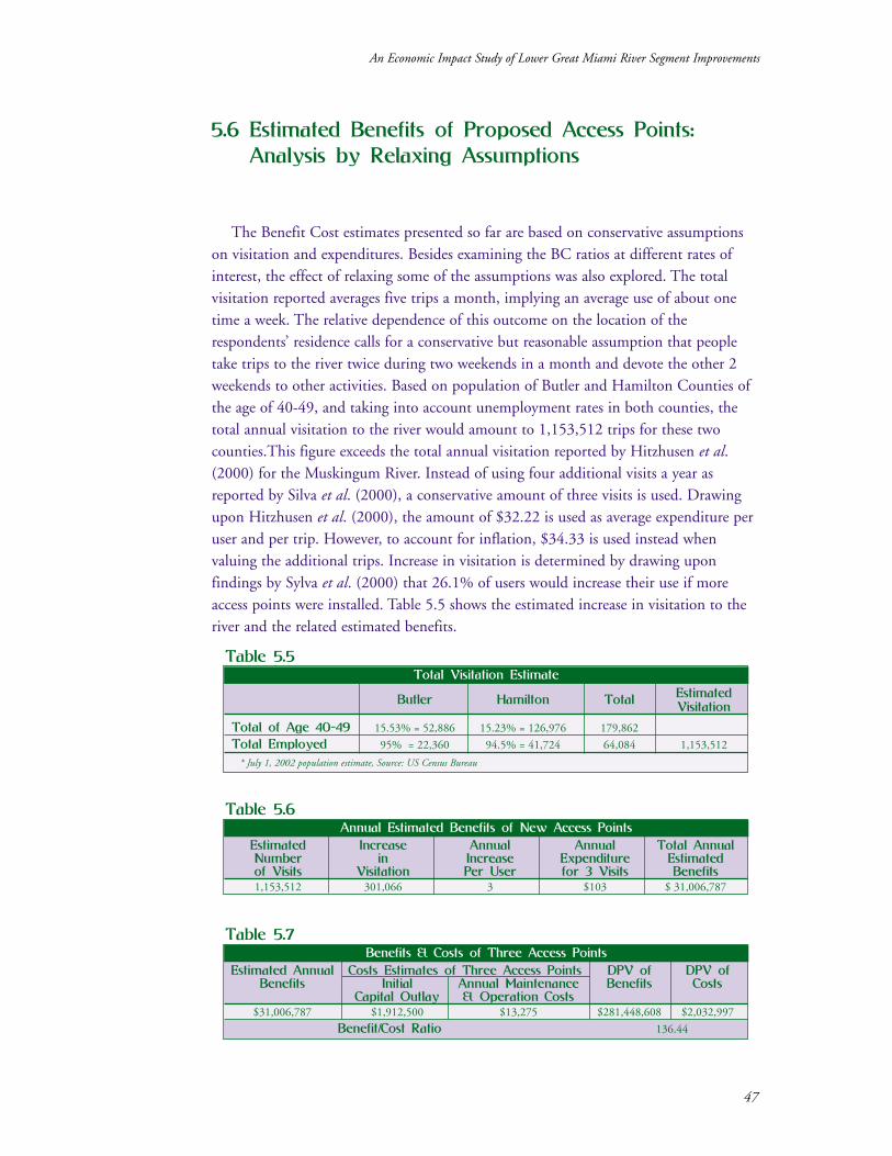
47


5.6 Estimated Benefits of Proposed Access Points: Analysis by Relaxing Assumptions

The Benefit Cost estimates presented so far are based on conservative assumptions

on visitation and expenditures. Besides examining the BC ratios at different rates of

interest, the effect of relaxing some of the assumptions was also explored. The total

visitation reported averages five trips a month, implying an average use of about one

time a week. The relative dependence of this outcome on the location of the

respondents’ residence calls for a conservative but reasonable assumption that people

take trips to the river twice during two weekends in a month and devote the other 2

weekends to other activities. Based on population of Butler and Hamilton Counties of

the age of 40-49, and taking into account unemployment rates in both counties, the

total annual visitation to the river would amount to 1,153,512 trips for these two

counties.This figure exceeds the total annual visitation reported by Hitzhusen et al.

(2000) for the Muskingum River. Instead of using four additional visits a year as

reported by Silva et al. (2000), a conservative amount of three visits is used. Drawing

upon Hitzhusen et al. (2000), the amount of $32.22 is used as average expenditure per

user and per trip. However, to account for inflation, $34.33 is used instead when

valuing the additional trips. Increase in visitation is determined by drawing upon

findings by Sylva et al. (2000) that 26.1% of users would increase their use if more

access points were installed. Table 5.5 shows the estimated increase in visitation to the

river and the related estimated benefits.

Table 5.5Total Visitation Estimate

Estimated Butler Hamilton TotalVisitation

Total of Age 40-49 15.53% = 52,886 15.23% = 126,976 179,862

Total Employed 95% = 22,360 94.5% = 41,724 64,084 1,153,512

* July 1, 2002 population estimate, Source: US Census Bureau

Table 5.7Benefits & Costs of Three Access Points

Estimated Annual Costs Estimates of Three Access Points DPV of DPV ofBenefits Initial Annual Maintenance Benefits Costs

Capital Outlay & Operation Costs$31,006,787 $1,912,500 $13,275 $281,448,608 $2,032,997

Benefit/Cost Ratio 136.44

Table 5.6Annual Estimated Benefits of New Access Points

Estimated Increase Annual Annual Total AnnualNumber in Increase Expenditure Estimated of Visits Visitation Per User for 3 Visits Benefits1,153,512 301,066 3 $103 $ 31,006,787

Sustaining a River

48

The BC ratio presented in Table 5.7 reports the discounted present value of benefits

and costs and the corresponding benefit/cost ratio, which is remarkably high, indicating

that the benefits outweigh the costs, suggesting that increasing access for in river

recreation in the Great Miami is a potentially high economic payoff investment.

However, it is imperative to mention here that the high Benefit Cost Ratio is not a true

indicator, but a possibility if the assumptions regarding the number of users and

expenditures are relaxed.

However, a number of issues remain to be addressed. Risk and uncertainty

associated with using the river may preclude boaters from increasing boating. For

example, in the event the water quality in the river deteriorates or boaters’ preferences

have changed, they may become less likely to increase boating even though new access

points have been built. Discontinuity of maintenance,difficulty of portaging around

dams, natural disasters, and changes in boating population may also represent

unpredictable factors that may affect the benefits. Therefore, in investigating the change

in boaters’ behavior due to installation of new access points, it would be important to

bear in mind the inhibiting factors that would prevent them from increasing their trip

to the river. Also adding the new access points may lead to congestion on the river

segments, implying some opportunity cost.

However, installing the new access points could be more beneficial to anglers. If no

fish are caught using a particular ramp, anglers could go somewhere else. The benefit

flows and costs may vary also during the lifetime of the new access points. Benefits may

be affected by location effects because river users could be from townships closer to the

river, relative distance of access points from nearest counties or townships may affect

the distribution of the economic benefits in those counties or townships.

Phot

o by

Rob

San

der

s

Only access point to Dravo Park canoe put-in area.

49

Section 6

Summary and Conclusions

...every river is a world of

its own, unique in pattern

and personality. Each mile

on a river will take you

further from home than a

hundred miles on a road.

-Bob Marshall

Phot

o by

Mar

ilyn

Wal

l

6.1 Summary and Conclusions

The need for research came from a request for economic valuation of benefits derived

from a natural resource, the Great Miami River. Township trustees, Miami Conservancy

District, citizens’ action groups such as Friends of the Great Miami River and Rivers

Unlimited wanted to explore possible solutions to enhance economic activity and

recreation in the river corridor. One of the objectives of the study was to estimate the

feasibility of buffer strip/zones along the river. Specifically, the goal was to determine the

impacts of gravel mining on residential property values. If gravel mining affected

property value, regulation of mining activity along the corridor would suggest a higher

tax base and revenue for the region, besides enhancing the scenic beauty of the river.

One of the objectives of the study was also to determine economic impacts of expanding

boating, fishing and other instream recreation opportunities by constructing new boat

ramps where needed to not only enhance the social capital of a given region but also to

boost the local economy and increase recreational opportunities for river users.

• The estimation of the costs and benefits of constructing a bike trail proved to be

a challenge since we did not have a benchmark for estimating these figures.

Besides, there was an ambiguity regarding the length and the location of the

bike way, since some properties located adjacent to the river were privately

owned residential, commercial and industrial parcels. Therefore, benefit transfer

values were simulated from the Heritage Trail, in Dubuque, Iowa, prepared by

Siderelis and Moore 1996. The trail extends for 27 miles, and estimates that on

average, per trip, a person spends approximately $11.09 on the bike trail. The

aggregate benefits relevant to the local economy from the bike trail are estimated

by multiplying the average amount spent by number of visitors per day. This

study develops a methodology to estimate opportunity cost of acquiring land for

the bikeway and buffer strips, and also develops methodology to estimate the

total Willingness to Pay, not just expenditures for construction of a bike trail.

• To estimate the impact of access points, again, the BT method was adopted.

A study by Kythrie Silva et al. (2000) which analyzed the behavior of Ohio

boaters at newly constructed ramps using a survey-based method was used as

the benchmark. The total annual visitation was estimated using benefit transfers

from a study on the Muskingum River. The goal was to assess the economic

benefits of installing new access points to the Great Miami River. Since applying

the benefit transfer method requires adjusting the benefit estimates based on the

policy site characteristics, the main problem encountered in conducting the

analysis was finding baseline data on the use of the Great Miami River. As a

result, a preliminary survey was administered. Rather than detailed estimates on

quantitative use of the river, the results of the survey give approximates of both

quantitative and qualitative characteristics of the river use.

51


For example, the type of activities for which people mostly use the river as well

as some inhibiting factors to additional use contingent on more access points

were identified.

Based on benefit transfers from previous studies and the results from the

preliminary survey, total estimated annual economic surplus of installing new

access points were a reasonable amount of $602,940. The analysis relies heavily

on a number of assumptions which when relaxed will yield different results.

One of such assumptions is that only three access points will be installed.

Using more access points in the calculation would change the benefit/cost

ratios presented in the sensitivity analysis. Further refinement of the analysis

can be made through a more comprehensive survey for which some insights in

terms of sample frame construction are collected from the preliminary survey.

• In case of the effect of gravel mining on property values, a hedonic pricing

method was used. The total decrease in property tax revenue accruing to the

local government from decreased property value resulting from proximity to

gravel mining is estimated at $2 million resulting in a tax revenue loss of more

than $100,000 annually to the local governments.

Sustaining a River

52

Phot

o by

Mar

ilyn

Wal

l

Indian Lake, the source of the Great Miami River.

6.2 Limitations of Research

There are some concerns about the accuracy and consistency of data in this research.

The parcel cards information provided by the auditors' offices in the two counties were

not uniform, in the sense that a singular method of classification was not followed by

the offices. Ideally, sale prices of properties taken over time would be the best choice for

the dependent variable. The number of sale transactions in the area was very limited;

therefore market-appraised values were used as a proxy. Concessionary sales were

deleted from the sample to rule out outliers.

For estimating marginal implicit prices and demand equations for the

environmental/community amenities, the variables have to be specified in natural

logarithmic form that requires that the variables are continuous, which was not

possible. We calculated approximate distance from gravel mines to the residential

properties, however, due to the presence of many gravel mines, several of them clustered

together, we had to adopt a binary form of identification, whether the parcel was

within one mile of a gravel mine or not.

The data used in the research are secondary data, thus some information regarding

the property owners was not available. More demographic and community variables

reflecting migration, school districts, crime rates might be instructive.

The sample contains only residential property parcels and not commercial and

industrial properties. Therefore, the results are at best lower bound estimates, and should

be interpreted accordingly. Some industrial properties such as gravel mining, weighing

and or processing plants may actually benefit from locating very close to the mine.

53


6.3 Further Research Needs

Several areas of potential further research can be identified. One of them is primary

data collection. The data could be improved if further and more in-depth research

could be carried out. Household demographics were not available from the parcel cards,

and hence could not be included in the data set. Using only county auditors' parcel

cards for measuring structural characteristics may have resulted in exclusion of some

important characteristics such as architectural features, landscaping, elevation of the

parcel, type of construction, other additions and built-in structures etc. Personal

interviews and individual assessments of homes would have allowed for more

information regarding septic system facilities and variation between homes. This would

allow for better estimates of the coefficients. With more time and financial resources,

this additional data collection would be advantageous to the study.

Further research on distance from river to parcels, and elevation/topography would

have resulted in a specification of a continuous variable for river proximity and

estimation of marginal implicit price for this variable.

Further research in estimating the second stage of the hedonic price function would

be beneficial in estimating gains and losses in total economic welfare. The different legal,

social, and institutional rules that are critical in understanding the regulation of gravel

mining, and ownership and stewardship of these industries could be useful. By using the

marginal implicit prices and income, a demand function for these amenities could be

estimated. Finally, the results from this research might be used to predict benefits

accruing from such improvements in other river systems in other parts of Ohio.

We look forward to discussing these results and further research implications with

interested parties in the Great Miami region.

Sustaining a River

54

55


Phot

o by

Mar

ilyn

Wal

lP

hot

o by

Mar

ilyn

Wal

l

Appendix 1:

Gathering Baseline Data on the Use of the Great Miami RiverStretch of Interest: Butler and Hamilton Counties

Focus Group

Purpose: It has been documented that the Great Miami River is underutilized due to lack

of access points. Assessing the benefits of increasing access to the river requires knowledge

about whether river users will increase their use if more access points become available. This

focus group (survey) is intended to shed light on this important question. Provided answers

will help decision makers allocate funds efficiently to river-related recreational activities.

All responses will be confidential. No individual responses will be reported, only the

average. No name is necessary.

Targeted People: Canoe club’s president and/or members, people living by the river,

township trustees, Miami Conservancy District, mayors of river villages, ODNR Division of

Wildlife, Watercraft and Natural Areas and Preserves, Friends of the Great Miami, and

others knowledgeable about the use of the river. These resource persons would be asked two

sets of questions. The first set is about themselves and the second set is about how they think

other people use the river.

Questions about the resource persons’ use of the river, if at all:

1. For which of the recreational purposes do you use the river the most?

Choose all applicable:

a) Walking/jogging b) Fishing

c) Boating (motorized and/or non-motorized) d) Tubing

e) Swimming f ) Kayaking

g) Hunting (lots of ducks) h) Canoeing

i) Biking on roads paralleling j) Sight seeing: 1) Bird watching

(some bikers ride their bikes across town and need to park) 2) Wild life viewing

k) Other_________________________________

2. a) In which months did you use the river last year?_______________________

b) How many trips did you take in these months?_______________________

3. How much money do you and your party members spend on average on a trip

(including, if any, charges for motel/hotel or camp) ?

4. Where do you purchase your trip supplies?

_____ close to your trip destination

_____ before you reach your trip destination?

57


5. What kind of trip supplies do you usually purchase? (Mark all applicable)

____Beverages _____Restaurant Food

_____Gas _____Lodging

_____Gear _____Groceries

_____Bait/Tackle _____Other (Please describe__________________)

6. Do you take trips to other segments of the river or to other river corridors?

__Yes __No

If yes, how many did you take last year ?__________

7. Which of the following best describes your household income?

a) Less than 10,000 b) 10,000 – 20,000

c) 20,000 – 30,000 d) 30,000 – 40,000

e) 40,000 – 50,000 f ) 50,000 – 60,000

g) 60,000 – 70,000 h) 70,000 and above

8. If you are using the river currently, would you respond to an increase in the access

to the river such as boat ramps, road access, and parking? If so, by how much

would you increase your use in a month you usually take trips?

9. Is there any change in the river or river corridor that would prevent you from

increasing your use of the river? If yes, please describe: _________________

____________________________________________________________

____________________________________________________________

10. Suppose you were asked to make a monetary donation as your one time

contribution to installing new access points, how much would you be willing

to donate? $_____________

11. Where would you suggest placing the access points? Identify Townships and

specific sites within townships; specify any reason for your location choice.

Townships:____________________ Specific Site:____________________

Reasons: ____________________________________________________

12. What if any infrastructure such as road, parking lots etc would be required in

conjunction with building the access point(s) at the location(s) you indicated

in the previous question?

13. What is your gender?

a) Male

b) Female

Sustaining a River

58

14. What is your home county and postal zip code? Please choose the one applicable

and specify the zip code

a) Butler _________Zip code

b) Hamilton __________Zip code

c) Other, please specify: ________________County ____________Zip code

Questions About Other River Users:

Choose all applicable:

a) Walking/jogging b) Fishing

c) Boating (motorized and/or non-motorized) d) Tubing

e) Swimming f ) Kayaking

g) Hunting (lots of ducks) h) Canoeing

i) Biking on roads paralleling j) Sight seeing: 1) Bird watching

(some bikers ride their bikes across town and need to park) 2) Wild life viewing

k) Other_________________________________

2. What would be your best guess about the number of river users at the Butler

and Hamilton county stretch?

- On a typical sunny week day _____________________________

- On a typical week-end day______________________________

3. Do you think people would increase their use of the river if more access points

were available? __Yes __No

If yes, by how much? _____________

4. What would be the best way to collect data on the use of the river?

Examples include:

a) Regular mail survey

b) Focus group

c) Other_________________

5. If we were to administer a mail survey, do you think we can get a list of the river

users and their addresses? If so, how and where?

59


References:

Alexander, G. R., and E. A. Hansen. “Sand Bed Load in a Brook Trout Stream.” North

American Journal of Fisheries Management (1986) 6:9-23.

Barksdale, R. D.. The Aggregate Handbook. National Stone Association, Washington,

D.C. 1991.

Bates, J. M.. “The Impact of Impoundment on the Mussel Fauna of Kentucky

Reservoir, Tennessee River.” American Midland Naturalist (1962) 68:232-236.

Bauer, A. M.. “Manipulating Mining Operations to Create Wildlife Habitats: a pre-

mining planning process.” Pages 41-43 in W. D. Svedarsky and R. D. Crawford,

editors. Wildlife Values of Gravel Pits. University of Minnesota Agricultural

Experiment Station, Miscellaneous Publication 17-1982, St. Paul, Minnesota 1982.

Benke, A. C.. “A Perspective on America’s Vanishing Streams.” Journal of the North

American Benthological Society (1990) 9:77-88.

Berkman, H. E., and C. F. Rabeni. “Effect of Siltation on Stream Fish Communities.”

Environmental Biology of Fishes (1987) 18:285-294.

Brown, A. V., M. M. Lyttle, and K. B. Brown. “Impacts of Gravel Mining on Gravel

Bed Streams.” Transactions of the American Fisheries Society (1998) 127:979-994.

Bull, W. B., and K. M. Scott. “Impact of Mining Gravel from Urban Streambeds in the

Southwestern United States.” Geology (1974) 2:171-174.

Cairns, J., Jr., K. L. Dickson, and E. E. Herricks. Recovery and Restoration of

Damaged Ecosystems. University Press of Virginia, Charlottesville, 1977.

Carling, P. A. “Deposition of Fine and Coarse Sand in an Open-work Gravel Bed.”

Canadian Journal of Fisheries and Aquatic Sciences (1984) 41:263-270.

Chang, H. H. “Modeling Fluvial Processes Instreams with Gravel Mining.” Pages 977-

988 in C. R. Thorne, J. C. Bathurst, and R. D. Hey, editors. Sediment Transport in

Gravel-bed Rivers. John Wiley, New York, 1987.

Chenoweth, R. E., W. G. Tlusty, and B. J. Niemann, Jr.. “Public Rights to Scenic

Resources: infringement is sufficient cause for denial of lowland sand and gravel

operations in Wisconsin.” Pages 73-79 in W. D. Svedarsky and R. D. Crawford,

editors. Wildlife Values of Gravel Pits. University of Minnesota Agricultural

Experiment Station, Miscellaneous Publication 17-1982, St. Paul, Minnesota, 1982.

61


Collins, B., and T. Dunne. “Gravel Transport, Gravel Harvesting, and Channel-bed

Degradation in Rivers Draining the Southern Olympic Mountains. Washington,

USA.” Environmental Geology and Water Science (1989) 13:213-224.

Collins, B., and T. Dunne. “Fluvial Geomorphology and River-gravel Mining: A Guide

for Planners, Case Studies Included.” Special Publication 98. California Department

of Conservation–Division of Mines and Geology, Sacramento, California, 1990.

Cross, F. B., F. J. DeNoyelles, S. C. Leon, S. W. Campbell, S. L. Dewey, B. D.

Heacock, and D. Weirick. “Impacts of Commercial Dredging on the Fishery of

the Lower Kansas River.” Report to the U.S. Army Corps of Engineers, Kansas City,

Kansas, 1982.

Desvouges,W. H., M. C. Naughton, and G. R. Parsons. “Benefit Transfer: Conceptual

Problem in Estimating Water Quality Benefit Using Existing Studies.” Water

Resources Research, (1992) 28:675-83.

Earnhart, Dietrich. “Using Contingent Behavior and Contingent Pricing Analysis to

Improve the Valuation of Travel Cost Components”. Department of

Economics–University of Kansas, 2000.

Feather P., Hellerstein D., and Hansen L., Economic Valuation of Environmental Benefits

and the Targeting of Conservation Programs: The Case of the CRP Agricultural Economics

Report No. 778. 64 pp, April 1999.

Heimlich R., Wiebe K., Claassen R., Gadsby D., and House R., Wetlands and

Agriculture: Private Interests and Public Benefits, Agricultural Economics Report No. 765.

104 pp, September 1998.

Hitzhusen, Fred. J., S. Lowder, and R. Ayalasomayajula. “Muskingum River Economic

Valuation”, Phase II Working Paper, Dept. of Agricultural, Environmental and

Development Economics–the Ohio State University, 2000.

Kondolf, G.M. “Hungry Water: Effects of Dams and Gravel Mining on River

Channels.” Environmental Management. (1997) 21(4):533-551.

Krunkilton, R. L.. “An Overview of Gravel Mining in Missouri and Fish and Wildlife

Implications.” Pages 80-88. Wildlife Values of Gravel Pits. University of Minnesota

Agricultural Experiment Station, Miscellaneous Publication 17-1982, St. Paul,

Minnesota 1982.

Loomis, J.B. and Walsh, R.G.. Recreation Economic Decisions. Comparing Benefits

and Costs. (2nd edition), State College, Venture Publishing, Inc. 1997, 440 p.

62

Sustaining a River

Martino J.. “The Precision of Delphi Estimates”. Technological Forecasting and Social

Change, (1970) 1(3), 293-99.

Nakao M, Sohngen B., Brown L. and Leeds R.. The Economics of Vegetative Filter Strips,

Fact sheet, AE -0006-99. (http://ohioline.osu.edu/ae-fact/0006.html).

Napier, Ted L.. “Watercraft Planning Study” Ohio Division of Natural Resources–

Division of Watercraft, 1994.

Nelson, E.L.. “Instream Sand and Gravel Mining.” Pages 189-196 in C.F. Bryan and

D.A. Rutherford, eds. Impacts on Warmwater Streams: Guidelines for Evaluation.

Southern Division–American Fisheries Society. Little Rock, Akansas, 1993.

Rosenberger, R. S. and J. B. Loomis. Benefit Transfer of Outdoor Recreation Use Values.

US Dept. of Agriculture–Forest Service, 2000.

Silva, Kythrie, K. Pisor, and F. J. Hitzhusen. “An Analysis of Boaters at Recently

Constructed ODNR Boat Ramps in Ohio”. ESO 2389 ODNR Pilot Project, Dept. of

Agricultural Economics–the Ohio State University, 1997.

Sommer, A.. “Determining the Value of Improved Water Quality in the Hocking River

Valley to Ohio Boaters and Fishers.” Thesis–Dept. of Agricultural, Environmental and

Development Economics–the Ohio State University, 2001.

63


515 Wyoming Avenue

Cincinnati, Ohio 45215

Phone: 513.761.4003

www.RiversUnlimited.org

Printed versions of this document were reproduced on Recycled Paper.

Please use recycled or tree-free paper if you print it yourself.

Please recycle this document when done.

an economic impact study of lower great miami river ... design and art direction: kevin pease, ......

Documents