an empirical signal separation algorithm for
TRANSCRIPT

An Empirical Signal Separation Algorithm for Multicomponent Signals Based on Linear
Time-Frequency Analysis
Lin Li 1, 2, *
, Haiyan Cai 2, Qingtang Jiang
2, Hongbing Ji
1
1 School of Electronic Engineering, Xidian University, Xi'an 710071, China
2 Department of Mathematics and Computer Science, University of Missouri-St. Louis, St. Louis 63121, United States
{lilin, hbji}@xidian.edu.cn, {haiyan_cai, jiangq}@umsl.edu
Abstract: The empirical mode decomposition (EMD) is a powerful tool for non-stationary signal analysis. It has been
used successfully for sound and vibration signals separation and time-frequency representation. Linear time-frequency
analysis (TFA) is another powerful tool for non-stationary signal. Linear TFAs, e.g. short-time Fourier transform (STFT)
and wavelet transform (WT), depend linearly upon the signal analysis. In the current paper, we utilize the advantages of
EMD and linear TFA to propose a new signal reconstruction method, called the empirical signal separation algorithm.
First we represent the signal with STFT or WT, and then by using an EMD-like procedure, extract the components in
the time-frequency (TF) plane one by one, adaptively and automatically. With the iterations carried out in the sifting
process, the proposed method can separate non-stationary multicomponent signals with fast varying frequency
components which will be mixed together when EMD is used. The experiments results demonstrate the efficiency of the
proposed method compared to standard EMD, ensemble EMD and synchrosqueezing transform.
Index Terms: time-frequency analysis; empirical mode decomposition; wavelet transform; signal separation.
1. Introduction
Separation of multicomponent non-stationary signals has broad applications in many engineering fields, such as
seismic signal analysis, vibration fault diagnosis, biomedical signal analysis, speech enhancement, sonar signal
processing, etc. The EMD algorithm along with the Hilbert spectrum analysis (HSA), introduced by Huang et al. in [1], is
an efficient method to decompose and analyze non-stationary signals. The EMD, considered as an adaptive signal
analysis, separates a given signal into a number of components, called intrinsic mode functions (IMFs), then calculates
the instantaneous frequency (IF) of each IMF by the HSA.
In recent years, efforts to improve the performance of EMD focus on envelope fitting, including interpolation
*Corresponding author
Email: [email protected]

algorithm and boundary expansion. In [1], the cubic spline function is used to generate the upper envelope and lower
envelope by interpolating the local maxima and local minima respectively. An alternative B-spline algorithm for the
EMD is introduced in [2]. And the blending cubic spline interpolation operator and corresponding error bounds are also
derived in [3]. The direct construction algorithm of envelope mean is proposed based on the constrained optimization for
narrow-band signals [4]. In addition, [5] proposes an alternative EMD using the filter to calculate the envelope mean. In
the iteration process, the boundary expansion error will gradually effect the accuracy of IMFs. Usually the symmetry rule
is used to predict the extrema beyond the two boundaries. A slope-based method is introduced to restrain the boundary
effect in [6].
The capability of EMD to decompose two sub-signals is discussed in [7], and the influence of sampling on the EMD
is discussed in [8]. And in [9], the EMD is considered as a filter bank, whose sub-band number, band-width and cutoff
frequency are adaptive and data-driven. An inverse filter scheme of EMD is proposed in [10], which aims to reduce the
scale mixing. The ensemble EMD (EEMD) proposed in [11], is a noise-assisted signal analysis method. EEMD utilizes
the advantage of the statistical characteristics of white noise to force the ensemble to exhaust all possible solutions in the
sifting process.
On the other hand, time-frequency analysis has been studied for many years, including linear TFA and non-linear
TFA, see the overviews in [12], [13], [14], [15] and [16]. Compared with EMD, TFA is of solid theoretical basis. The
research tendency of TFA is to enhance the TF resolution and energy concentration. The uncertainty principle [16] makes
a tradeoff between temporal and spectral resolutions unavoidable. To overcome this important shortcoming, the
time-frequency reassignment method is used to produce a better localization of signal components [17]. The
synchrosqueezing transform (SST) is introduced in [18] and further developed in [19]. SST is a special type of
reassignment method on the continuous wavelet transform (CWT) to enhance the energy concentration of the
time-frequency plane. The sub-signals are reconstructed by extracting the IF curves in the SST plane one by one. SST
works well for single-tone signals, but not for broadband time-varying frequency signals. The generalized SST and
instantaneous frequency-embedded SST (IFE-SST) are proposed in [20] and [21] respectively, with both of them
changing broadband signals to narrow-band signals and IFE-SST preserving the IFs of the original signals. A
multitapered SST is introduced in [22] to enhance the concentration in the TF plane by averaging over random
projections with synchrosqueezing. A hybrid EMD-SST scheme is introduced in [3] by applying the modified SST to the
IMFs obtained by the EMD. STFT-based SST is discussed in [23] and [24], and STFT-based second-order SST is
proposed in [25]. The matching demodulation transform and its synchrosqueezing are discussed in [26]. The linear and
synchrosqueezed time-frequency representations are reviewed in [27] in detail.

In this paper, we utilize the advantages of EMD and linear TFA to propose a new signal separation method, called the
empirical signal separation algorithm (ESS). In the sifting procedure of EMD, only features in time domain, e.g.
maximum and minimum extrema are used to decompose the given signal. So EMD is sensitive to noises and usually
results in mode mixing and artifacts. Based on linear TFA (STFT or WT), we use an EMD-like algorithm to extract the
signal components in the TF plane one by one. Our algorithm is different from the empirical wavelet transform in [28],
which extracts the components by designing an appropriate wavelet filter bank. Compared with the signal reconstruction
by SST, our algorithm is adaptive and can be used for multicomponent signals dissatisfying the adaptive harmonic model
(AHM) in [3]. The remainder of this paper is organized as follows. The linear TFA and SST are reviewed in Section 2.
The ESS is introduced in Section 3. We also discuss some properties of ESS in Section 3. The numerical results and
comparisons are provided in Section 4.
2. Linear Time-Frequency Analysis and Synchrosqueezing Transform
A multicomponent amplitude and frequency-modulated (AM-FM) signal is given by [16],
1 1
( ) ( ) ( )cos 2 ( )N N
j j j
j j
s t s t A t t
where ( )s t consists of N monocomponent signals. To allow for the extraction and separation of components from a
given signal, the IF of the j-th component ( ) ( )cos 2 ( )j j js t A t t is ( )j t , and the amplitude ( )jA t and the IF
( )j t are positive, slowly varying compared to ( )j t .
2.1. The Linear Time-Frequency Analysis
Let us start with the short-time Fourier transform (STFT). For a real-valued window function 2u L with unit
norm, and a signal 2s L , the STFT of ( )s t is defined by,
, i
sV t s u t e d
for ,t , where t and denote time and angular frequency, respectively. Note that 2 , where is the
frequency.
When the Gaussian function
2
21
2
t
u t e
with 1 4 is used as the window function, the STFT is called the Gabor transform [24].
The signal ( )s t can be reconstructed by the inverse STFT, using the following formula,
2
( ) , i t
ss V t u t e dtd
And ( )s t can also be reconstructed by
1
( ) ,(0)
ss t V t du
Note that ( )u t is required to be non-zero and continuous at 0, see [23].
Now we discuss the TF resolution of STFT. The time center of the window function ( )u t is defined by
2
2
( )
( )u
t u t dtt
u t dt
and the equivalent duration of ( )u t is defined by
1
2 22
2
( )
( )
u
u
t t u t dt
u t dt
The Fourier transform of ( )u t is denoted by ˆ( )u . Then the frequency center and equivalent bandwidth of ( )u t
are denoted as u and
u , obtained by Eq. (6) and Eq. (7) with u and t replaced by u and , respectively.
From the Heisenberg uncertainty principle, we have ˆ
1
2u u , and the equality is obtained for Gaussian function only,
see details in [16]. u and
u are also called temporal and spectral resolutions, respectively. The uncertainty
principle imposes an unavoidable tradeoff between temporal and spectral resolutions.
CWT is another method of linear TF analysis. Like STFT, CWT uses a window to locate a signal to its time and
frequency content. However, the window shape of CWT changes continuously at different frequency instant.
Let 2( ) ( )t L be a fix function. ˆ( ) is the Fourier transform of ( )t . If satisfies the conditions,
ˆ( ) 0 for 0
2
0
ˆ0 ( )d
C
then ( )t is called an analytic wavelet.
Let us denote ( , ) ( )a b t as the corresponding family of wavelet ( )t ,
( , )
1( )a b
t bt
a a
where 0a is the scale, and b is the shift. The Fourier transform of ( , ) ( )a b t is written as

( , )ˆ ˆ( ) i b
a b a e
The CWT of a signal 2( ) ( )s t L is defined by
1
,, , ( )s a b
t bW a b s s t a dt
a
An analytic signal ( )s t can be recovered from ( , )sW a b by (see e.g. [31], [32] and [33])
1
,0
1,s a b
s t W a b a t dbdaC
For an analytic CW ( )t , if 0
ˆ( )C d
, another reconstruction formula can be alternatively used
(see [18] and [19]),
1
0
1( ) ,ss b W a b a da
C
For real signals, the CWT with integral involving b is invertible too. Let 2s L be a real-valued signal.
Consider the analytic signal with associated s , which is denoted by
( ) ( ) ( ) ( )as t s t i s t
where ( )s is the Hilbert transform of s . The following reconstruction formulae exist in 2 ( )L [19],
1
,0
2( ) ,s a b
s t e W a b a t dbdaC
1
0
2( ) ,ss b e W a b a da
C
With the definitions in Eq. (6) and Eq. (7), we can also calculate the temporal and spectral resolutions of wavelet
( , )a b , which are given by
,
,
12 22
2
1
1
a b
a b
t bt t dt
a aa
t bdt
a a
,
,
12 22
ˆ
ˆ ˆ2
ˆ1
ˆ
a b
a b
i b
i b
a e d
aa e d

Time (s)
Fre
quency (
Hz)
0 100 200 300 400 5000
0.1
0.2
0.3
0.4
0.5
Time (s)
Scale
0 100 200 300 400 500
3.5
12
42
150
510
Figure 1. The STFT (left) and CWT (right) of a LFM signal
where and
are the temporal and spectral resolutions of the mother wavelet, respectively, ,a b
t and
,ˆ
a b
are the centers of ,a b and ,
ˆa b
, respectively. Therefore, we obtain
, ,
ˆ ˆ
1
2a b a b
where the equality is obtained for the Gaussian function only.
From Eq. (18), Eq. (19) and Eq. (20), we know the localization window of ( , )a b is not fixed when CWT is used.
For larger a , viz. the low frequency band, it provides a narrower frequency window and hence a higher frequency
resolution, but a lower time resolution. On the other hand, the opposite is true. Figure1 shows the difference between
STFT and CWT. The simulation signal is a linear frequency modulation (LFM) signal, where the frequency changes
linearly from 0.02Hz to 0.2Hz.
2.2. The Synchrosqueezing Transform
Based on the linear TFA above, the SST is a TF reassignment approach, which aims to sharpen the TF representation
while keeping the temporal localization. SST has been proved to be well adapted to multicomponent signals in [19].
However, it is difficult to separate an unknown multicomponent signal to specific components without any prior
knowledge and/or appropriate restrictions. Eq. (1) is called the AHM [3], with the restrictions described by
1 2
1 2
1 2
( ) ( ); ( )
inf ( ) ; sup ( )
inf ( ) ; sup ( )
( ) ( ); ( ) ( )
j j
j jt t
j jt t
j j j j
A C L C
A t c A t c
t c t c
A t t t t
for all t , where 0 1 and 1 20 c c . In addition, the components are said to be well-separated if
1
1 1
( ) ( ),
( ) ( ) ( ) ( ) ,
j j
j j j j
t t
t t d t t

for all t and some 0 1d . A continuous function ( ) ( )cos 2 ( )f t A t t with ( )A t and ( )t satisfying
conditions (21) and (22) is called an intrinsic mode type (IMT) function in [19].
The CWT-based SST (WSST) works through squeezing the CWT, where the wavelet is required to be admissible
(defined in Eq. (9)). The reference IF function (local IF) based on CWT is defined by,
,,
2 ,
b s
s
s
i W a ba b
W a b
Then the WSST is defined by
1
: ,, , ,
s
s s sa W a b
T b W a b a b a da
where 0 , which is used to reduction numerical error and noise influence (see the discussions in [18] and [19]).
Similar to the WSST, the STFT-based SST (FSST) works through squeezing the STFT. The local IF is defined by
[23]
,,
2 ,
t s
s e
s
i V tt
V t
Then the FSST is defined by
: ,
1, , ,
(0) s
s s sV t
P t V t t du
The SST is used not only to sharpen the TF representation, but to separate the multicomponent signal into its
constituent modes. For a multicomponent signal in [1], the j-th component can be reconstructed by WSST and FSST,
respectively:
0
1( ) lim ,
j
j sb
s b T b dC
0
( ) lim ,j
j st
s t P t d
where is the width of the zone to be summed up around the ridge corresponding to the IF of the j-th component.
3. The Empirical Signal Separation Algorithm
Let us start with the squeezing and recovery of a monocomponent signal by SST. Consider
1
0.08( ) cos 2 0.11 cos 0.01
0.01x t t t
where 1 is the random initial phase. ( )x t is a sinusoidal frequency modulation signal which can be found in radar
systems. Figure 2 shows one of the waveform of signal ( )x t and its IF. Note the sampling frequency is 1Hz.
0 100 200 300 400 500
-1
-0.5
0
0.5
1
Time (s)
Am
plit
ude
0 100 200 300 400 5000
0.05
0.1
0.15
0.2
0.25
Time (s)
Fre
quency (
Hz)
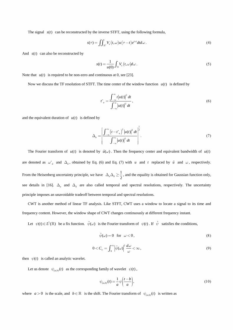
Figure 2. Waveform of signal ( )x t (left) and its instantaneous frequency (right).
Time (s)
Scale
0 100 200 300 400 500
3.5
12
42
150
510
Time (s)
Fre
quency (
Hz)
0 100 200 300 400 5000
0.1
0.2
0.3
0.4
0.5
Time (s)
Fre
quency (
Hz)
0 100 200 300 400 500
0.006
0.018
0.054
0.17
0.5
Time (s)
Fre
quency (
Hz)
0 100 200 300 400 5000
0.1
0.2
0.3
0.4
0.5
0 100 200 300 400 500
-0.5
0
0.5
Time (s)
Am
plit
ude
0 100 200 300 400 500
-1
-0.5
0
0.5
Time (s)
Am
plit
ude
Figure 3. CWT (top left) and STFT (top right) of ( )x t , WSST (middle left) and FSST (middle right) of ( )x t , the waveform
reconstructed from WSST (bottom left) and the waveform reconstructed from FSST (bottom right).
Figure 3 shows the SST and the waveform reconstruction results by the Synchrosqueezing Toolbox by E. Brevdo and
G. Thakur [19, 24, 29]. The wavelet used is Morlet’s wavelet with parameters 1 and 2 and the number of
voices used is 64. The window function for STFT is the standard Gaussian, with parameters mean 0 and standard

deviation 0.12. The threshold in both WSST and FSST is equal to 310 . The width of the zone to be summed up
around the ridge for waveform reconstruction is 5 (the discrete form, unitless), for both WSST and FSST. We find
that the SST works well when the IF changes slowly, but not well when the IF changes fast. See WSST and FSST in
Figure 3. This can also be found in the recovered waveforms, see the bottom row in Figure 3. Theoretically, for a
monocomponent signal, one can increase the width to improve the recovery performance. However it is not always
this to process multicomponent signals since increasing the width will result in the mixture of components.
3.1. Signal Recovering by Linear Time-Frequency Analysis Directly
Consider the IMT function ( ) ( )cos 2 ( )s t A t t , the CWT of ( )s t is approximated by
2 ( )1 ˆ, ( ) 2 ( )2
i b
sW a b A b e a b
For a single-tone signal ( ) cos 2s t A ct , especially, its CWT is given by
21 ˆ, 22
i bc
sW a b Ae ac
If the center frequency of ˆ( ) is 0 , ,sW a b will concentrate around
0 (2 )a c . The IF function of ( )s t
is ,s a b c . Then by Eq. (24), all points ( , )a b in CWT plane can be "squeezed" to ( , )c b in the WSST plane.
However, if there is a significant change of frequency in the signal, the efficiency of synchrosqueezing of IF depends on
the instantaneous bandwidth of signal in the range of the analysis wavelet. Looking back at Figure 3, synchrosqueezing
performs well near the extrema of IF of the original signal, where the IF changes slowly.
Note that by increasing the width and using second-order SST, we can enhance the accuracy of the
reconstruction waveform continuously in Figure 3. However, the important problem is how to deal with the
multicomponent signals. Next, let us consider another numerical example given by
1 2 3
1 2 3
( ) ( ) ( ) ( ) ( )
cos 0.12 10cos(0.006 ) cos 0.22 10cos(0.006 ) cos 0.38 ( ),
y t s t s t s t n t
t t t t t n t
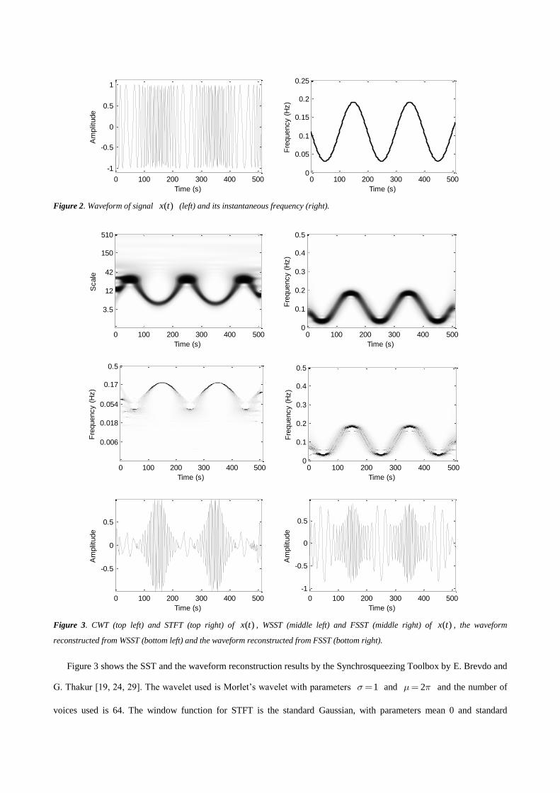
where ( )n t is an additive noise. Figure 4 shows the IFs of the three components in ( )y t and also the mixed waveform
with an additive Gaussian white noise. The sampling rate is 1Hz and the signal duration is from 0s to 511s. Observe that
3 ( )s t starts at 65s and ends at 384s.
Figure 5 shows the CWT, STFT, WSST and FSST of the multicomponent signal ( )y t , respectively. The
corresponding parameters of these algorithms are the same as those used in Figure 3. Note that both WSST and FSST do
not work well for the two sinusoidal frequency modulation signals. It seems FSST is better than WSST in Figure 5. But
when changing the wavelet parameters in WSST, we can obtain better representation for either the high frequency
component 3 ( )s t or the low frequency component
1( )s t . When using SST to extract the components, we need to know
exactly the number of components and the width of extraction window first. So it is not adaptive.
Actually, we can use the CWT or STFT to recover a signal too, see Eq. (5) and Eq. (14). But for multicomponent
signal, the recovering algorithm based on CWT or STFT is also not adaptive. [27] indicates that the synchrosqueezed
transform cannot improve TF resolution of STFT and CWT in the sense if the components are not reliably represented by
STFT or CWT, then they will not be well separated by SST. By comparing the results in Figure 3 and Figure 4, and our
other experiments, we find that the CWT and STFT are more stable than WSST and FSST in the whole TF plane.
0 100 200 300 400 5000
0.1
0.2
0.3
0.4
0.5
Time (s)
Fre
quency (
Hz)
0 100 200 300 400 500
-2
0
2
Time (s)
Am
plit
ude
Figure 4. The real IF of ( )y t (left) and the waveform with signal-to-noise ratio (SNR) 15dB (right).
Time (s)
Scale
0 100 200 300 400 500
3.5
12
42
150
510
Time (s)
Fre
quency (
Hz)
0 100 200 300 400 5000
0.1
0.2
0.3
0.4
0.5
Time (s)
Fre
quency (
Hz)
0 100 200 300 400 500
0.006
0.018
0.054
0.17
0.5
Time (s)
Fre
quency (
Hz)
0 100 200 300 400 5000
0.1
0.2
0.3
0.4
0.5
Figure 5. Analysis of multicomponent signal ( )y t : real part of CWT (top left), real part of STFT (top right), WSST (bottom left) and
FSST (Bottom right).

3.2. Extraction of TF Ridges
Considering the AHM conditions and noise effect, we use the extrema of the real part and imaginary part of STFT or
CWT to extract the TF ridges. We take CWT as example in the following analysis. Suppose ( ) ( ) ( )f t s t n t , where
( )n t is a white noise with mean 0 and variance 2
n , and ( ) ( )cos 2 ( )s t A t t is an IMT function. The CWT of
( )f t is given by
2 ( )
, , ,
1 1ˆ( ) 2 ( ) ( ) .2
f s n
i b
W a b W a b W a b
t bA b e a b n t dt
a a
The expectation and variance of ,fW a b are given by
2 ( )1 ˆ, , ( ) 2 ( )2
i b
f sE W a b W a b A b e a b
and
2,f nVar W a b C a
where ( )C a varies with scale a . See Appendix A for the proofs of Eq. (35) and the following Eq. (36) and Eq. (37).
Suppose 1 1,a b is a point on which ,se W a b gains its local extreme value. The signal-to-noise ratio of
1 1,fe W a b is defined by
2
1 1
1 1 1
1 1
,( , )
,
s
f
e W a br a b
Var e W a b
and we have
2
1 1 1
1 1 1 2
1
ˆ( ) 2 ( )( , )
n
A b a br a b
C a
Analogously, the signal-to-noise ratio of 1 1,fW a b is
22
1 1 11 1
2 1 1 1 1 12
11 1
ˆ( ) 2 ( ), 1( , ) ( , )
22,
s
nf
A b a bW a br a b r a b
C aVar W a b
Note that for imaginary part Im ,fW a b , the signal-to-noise ratio is the same as Eq. (36) with e replaced by
Im , where 1 1,a b is a local extreme point of Im ,sW a b . Furthermore, the absolute operation is nonlinear, which
means that the extracted ridge is not always consistent and unbiased for the IF estimation. After we extract the extrema of
the real part and imaginary part first, we use the cubic spline to interpolate the extema to obtain the ridge of IF.

3.3. Effect of the Window/Wavelet Parameters
Unless otherwise noted, the wavelet used in the remainder of this paper is Morlet’s wavelet. Morlet’s wavelet is
composed of a complex exponential multiplied by a Gaussian window, given by
2 2 2
2
1 1
2 2,( )
ti tt c e e e
where , 0 ,c is a normalizing constant subject to
2( ) 1t dt
Then we have
2 2
2 2
11 1 3 24 2 4
, 1 2c e e
The Fourier transform of Morlet’s wavelet is given by
22 2 2 21 11
2 2 22,
ˆ( ) 2c e e
Note that 2
ˆ( ) 2d
.
The frequency center of ( )t is given by
2 2
2 22 2
2 3
4
ˆ 32
4
ˆ( ) 1
ˆ( ) 1 2
d e
d e e
The bandwidth of ( )t is given by
2 22 2
2 22 2
11 3 2
2 2 2 22 42 2 2ˆ
ˆ 32
4
1 1 1 12ˆ
12 2 2 4
2ˆ1 2
e ed
d e e
Usually, we let and 0.5 , then
. Therefore, the center and bandwidth of ˆ( ) are dependent on
and , respectively. In addition, by Eq. (18) and Eq. (19), we have,
,
,
ˆ ˆ
11 2 ,
2 .
a b
a b
aa
a a
By Eq. (31) and Eq. (42), CWT ,sW a b of a single-tone signal ( )s t with Morlet’s wavelet will concentrate
around (2 )a c , with scale support zone
1 1 1 1
2 22 2
2 2a
c c

For a multicomponent signal with pure harmonics 1
( ) cos 2K
k k
k
s t A c t
, where 0kA and 1k kc c , to
separate each component with CWT, the wavelet should satisfy
1
1 2 2 1 2 2
2 2k kc c
for all 1k , which is equivalent to
1
1
1
2 2
k k
k k
c c
c c
Thus it seems that the bigger value of comes better separation of a multicomponent signal in the CWT plane.
However, this conclusion may only correct for pure harmonics. To this regard, let us consider a linear frequency
modulation signal
2( ) cos 22
rs t A ct t
with phase 2( )2
rt ct t , instantaneous frequency ( )t c rt and chirp rate ( )t r . Then its scale support
zone is
2 2
2 2
h hac rt c rt
where 2
2 2
2
1 12
2h ra
, see the proof in the Appendix B.
Suppose 1k kc c and
1 1 0k k k kc r t c r t . To separate each component with CWT, the wavelet should
satisfy
1
1 1
2 2
2 2
k kh h
k k k kc r t c r t
Consider 1kh
and kh on the ridge
1
1 1
( )2
k
k k
a tc r t
and
( )2
k
k k
a tc r t
, respectively, we have
2 24 41
4 42 2
1 1
1 1
11 1
2 2 4 4
2 2
k k
k k k k
k k k k
r r
c r t c r t
c r t c r t
Note that Eq. (49) is a fourth order inequality with respect to , where 0 . So Eq. (49) may hold for
some specific intervals on of .
Therefore, by selecting different the parameters and , we can change the position of the ridge in the CWT
plane, and hence change the scale support zone around the ridge. The width of scale support zone depends on both the
bandwidth of ,a b and the instantaneous bandwidth of the signal to be analyzed. For a monocomponent signal, we

Time (s)
Scale
0 100 200 300 400 500
3.5
12
42
150
510
Time (s)
Scale
0 100 200 300 400 500
3.5
12
42
150
510
Time (s)
Scale
0 100 200 300 400 500
3.5
12
42
150
510
Time (s)
Scale
0 100 200 300 400 500
3.5
12
42
150
510
Figure 6. CWTs of ( )y t with different parameter: , 1 (top left), 4 , 1 (top right), 2 , 0.5
(bottom left) and 2 , 2.5 (bottom right).
should choose suitable and to make sure the CWT is well concentrated and its ridge keeps away from the upper
and lower bound of the CWT plane (finite discrete). For a multicomponent signal, except for the conditions above, we
need to separate different components as well as possible.
Take the noise-free multicomponent signal in Figure 4 ( ( )y t in Eq. (32) with ( ) 0n t ) for example. Figure 6
shows the CWT with different parameters. When 1 , increases from to 4 , the distribution moves from the
bottom to the top in the CWT plane. On the other hand, when 2 , increases from 0.5 to 2.5 , the distribution
holds at the same position but with increasing frequency resolution for the low frequency component. From the left
column of Figure 6, we find that the component with lowest frequency is well-represented, but the components with high
frequency are not concentrated. On the other hand, from the right column of Figure 6, the two components with high
frequency are well-represented, but the component with the lowest frequency is not concentrated. That means we cannot
obtain a good representation for both high frequency component and low frequency component simultaneously for CWT
and SST.
3.4. CWT-based and STFT-based empirical signal separation
Based on the above discussions, we utilize the advantage of EMD to extract the signal components adaptively. The
conventional EMD only uses the features in time domain, e.g. maximum and minimum extrema to decompose a signal.
Here, we present a new EMD-like method by sifting in the TF plane. We need no prior knowledge of the signal to be
decomposed. The new method is more efficient to separate components close to each other than EMD and SST as

demonstrated in the experiment results in Section 4. The proposed algorithms are called CWT-based empirical signal
separation (CWT-ESS) algorithm and STFT-based empirical signal separation (STFT-ESS) algorithm.
In our method, different signal components are extracted by changing the parameters of Morlet’s wavelet
automatically. Because the higher frequency component always has the ridge with narrower bandwidth when using a
suitable window (see figure 6), namely high energy concentration, so we first extract the high frequency component with
maximal amplitude. We use the frequency spectrum to determine the value of parameters adaptively.
Suppose the effective frequency range of the signal is [ , ]p q with 0 1 2p q , and the sampling rate is 1 Hz.
Actually, one can use the principle of 3-dB bandwidth to find p and q , which are given by
0
0
ˆ ˆmin : arg ( ) ( ) 2 ,
ˆ ˆmax : arg ( ) ( ) 2 ,
p f f
q f f
where f is the Fourier transform of f t , and 0ˆarg max ( )f
. Suppose the signal length is N ( N is a
power of 2, namely 2 ,mN m ) and the number of voice is vn . We choose a proper to make the Morlet’s
wavelet transform of the signal distribute in the center of the CWT plane. Because the domain of the scale is
{ 2 , 1,2, , }vk n
k va k mn with sample frequency 1Hz, we define the center area (half) of the CWT with the scales
{ 2 : 4, 4 1, ,3 4}vk n
k v v va k mn mn mn for example. Then by (2 )a c in Eq. (43), we calculate
3 4
1
4
2
2 2 ,
2 2 .
m
m
p
q
Here to avoid unexpected errors, we set the range of to be [ ,5 ] , namely,
1 2 1 2
1 2
max ( ) 2, , if ( ) 2 5 ;
5 , if ( ) 2 5 .
By Eq. (45) or Eq. (49), we could determine the range of theoretically. But since we have no prior information
about the input signal, such as number of components, instantaneous frequency etc. We choose 1 as in [19] for
simplification.
Next we calculate the CWT. After that, based on Section 3.2, we find an extreme point (with absolute value exceeds a
given threshold 1 ) which is closest to the line of scale 1a and time 2b N in the CWT plane. Then we find
extrema belong to the same component next to the current point one by one. Note that extrema of the real part and the
imaginary part, the maximum and the minimum, are always being alternately along the time line. And the interval

between two adjacent extrema varies slowly according to the AHM. With these conditions, we can to extract all the
maximum and minimum extrema from one component.
Now we present the steps of the CWT-ESS for a given signal ( )f t .
First, initialize 1k , ( ) ( )r t f t ,
Step 1: Determine the window/wavelet parameters.
Using the Fourier transform to calculate the start and cut frequencies of the signal ( )r t , namely kp and kq . Then
determine the values of k .
Step 2: Extract the maximum and minimum extrema of the high frequency component in the CWT plane (both real
part and imaginary part).
Step 3: Interpolate the extrema by the cubic spline, and extract the slice ( )c t on the interpolation ridge ( )kd t in
the CWT plane.
0ˆ( ) 2 ( ), ( )f kc t e W d t t
0( ) ( )k km t d t
where ( )km t is the IF of the k-th IFM, and 0 for Morlet’s. Then iterate (stop when satisfy the stop criterion), and
obtain the k-th IFM.
Step 4: For the residual r , let 1k k , f r , repeat Step 1~3, obtain the other IFMs. ■
The stop criterion for Step 3 is that when 2OS (
2 1.01 in this paper), stop iterating [5].
1
1
( ) ( )
( ) ( ) ( )
k lt
k lt
imf t c tOS
f t imf t c t
where ( )kimf t and 1( )lc t are defined in Algorithm 1.
Note that when the STFT is used, Eq. (53) and Eq. (54) are replaced by
1
( ) ( ),(0)
f kc t V d t tu
and
( ) ( )k km t d t
Furthermore, because of the equal TF resolution in the whole STFT plane, we simply use a constant window for
STFT-ESS, which means we will ignore Step 1.

Algorithm 1
Input ( )f t , let ( ) ( )r t f t , 1k .
Iteration:
1,l 0kimf t , ( ) ( )lr t r t .
Calculate kp , kq , then
k , ,lr
W a t .
While 1max ( , )lr
W a t , do
Calculate the interpolation ridge ( )kd t ,
0ˆ( ) 2 ( ), ( )
ll r kc t e W d t t , ( ) ( ) ( )k k limf t imf t c t , 1( ) ( ) ( )l l lr t r t c t
11 0
ˆ( ) 2 ( ), ( )ll r kc t e W d t t
.
While 2OS , do
1l l ,
0ˆ( ) 2 ( ), ( )
ll r kc t e W d t t , ( ) ( ) ( )k k limf t imf t c t , 1( ) ( ) ( )l l lr t r t c t ,
11 0
ˆ( ) 2 ( ), ( )ll r kc t e W d t t
.
( ) ( )lr t r t , 1k k .
4. Numerical results
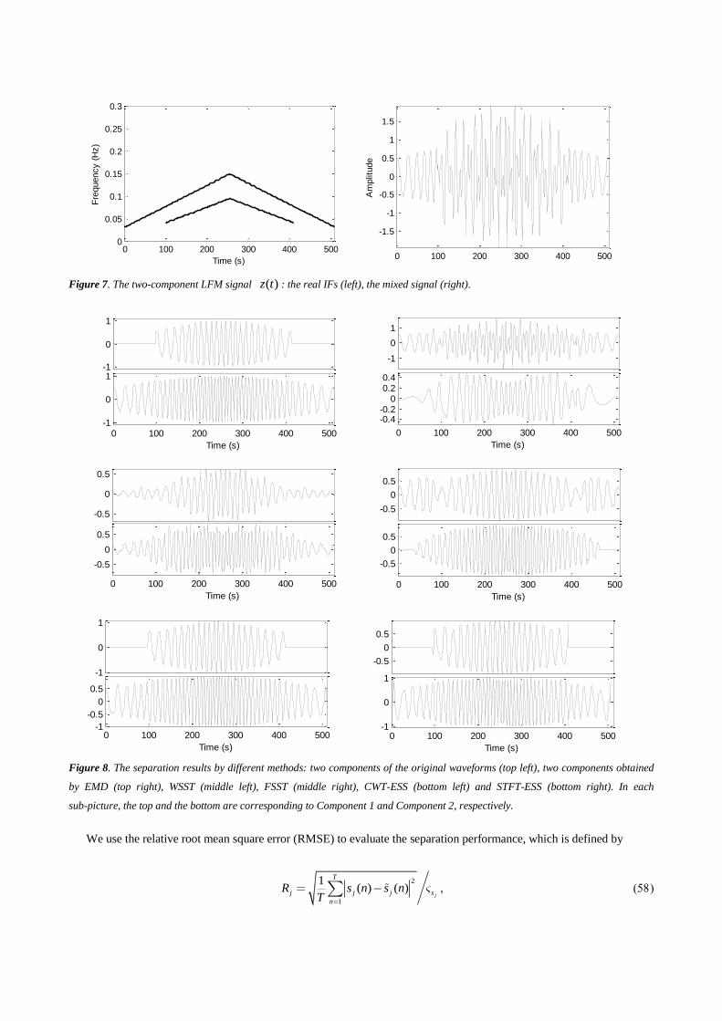
In this section, various numerical examples are used to validate the proposed methods. First we deal with the
two-component non-stationary signal ( )z t in Figure 7. Component 1 has the low frequency, while Component 2 the
high frequency. Both of their amplitudes are modulated symmetrically by the Gaussian functions, see the original
waveforms in Figure 7. And their frequency modulations are symmetrical triangular LFM. The waveforms are
continuous.
Figure 8 shows the separation results by different methods. Note that the parameters of WSST and FSST algorithms
are the same those in Figure 3 and Figure 5. In addition, the number of components and the width of extraction window
are set in advance to be 2 and 5, respectively. We just display the first IMF and second IMF of the decomposition results
of EMD by using the code supplied by T. Oberlin [4]. Because of the “mode mixing” (as explained in [7]), EMD cannot
separate these two components. For CWT-ESS and STFT-ESS, also we just display the first two modes. By comparing
the waveforms of the separation results to the original ones, we can find that our methods are superior to the EMD,
WSST and FSST.
0 100 200 300 400 5000
0.05
0.1
0.15
0.2
0.25
0.3
Time (s)
Fre
quency (
Hz)
0 100 200 300 400 500
-1.5
-1
-0.5
0
0.5
1
1.5
Am
plit
ude
Figure 7. The two-component LFM signal ( )z t : the real IFs (left), the mixed signal (right).
-1
0
1
0 100 200 300 400 500-1
0
1
Time (s)
-1
0
1
0 100 200 300 400 500
-0.4-0.2
00.20.4
Time (s)
-0.5
0
0.5
0 100 200 300 400 500
-0.5
0
0.5
Time (s)
-0.5
0
0.5
0 100 200 300 400 500
-0.5
0
0.5
Time (s)
-1
0
1
0 100 200 300 400 500-1
-0.5
0
0.5
Time (s)
-0.5
0
0.5
0 100 200 300 400 500-1
0
1
Time (s)
Figure 8. The separation results by different methods: two components of the original waveforms (top left), two components obtained
by EMD (top right), WSST (middle left), FSST (middle right), CWT-ESS (bottom left) and STFT-ESS (bottom right). In each
sub-picture, the top and the bottom are corresponding to Component 1 and Component 2, respectively.
We use the relative root mean square error (RMSE) to evaluate the separation performance, which is defined by
2
1
1( ) ( )
j
T
j j j s
n
R s n s nT

where ( )js n is the reconstruction of ( )js n , js is the standard deviation of ( )js n , and ( )js n is the j-th component
of a multicomponent signal.
Figure 9 shows the relative RMSE under different signal-to-noise ratios (SNRs) for the two-component triangular
LFM signal ( )z t . The additive Gaussian white noises are added to the original signal with SNR from 10 to 20 dB.
Under each SNR, we use the Monte-Carlo experiment for 100 runs. Note that the parameters for recovering with WSST
and FSST are the same as Figure 8. Because of noises, here we use the EEMD [11] instead of EMD. And for the EEMD,
it repeats 200 times for average by adding independent noises with standard deviation 0.1. Obviously, from the results in
Figure 9, the algorithms CWT-SST and STFT-SST introduced in this paper are superior to EEMD, WSST and FSST.
Then, we move to the three-component signal ( )y t in Eq. (32), whose IFs and waveform are shown in Figure 4, and
WSST and FSST are shown in Figure 5. Because the SST based reconstruction methods are supervised which requires
the input of the number of components of the signal and the parameter, the separation performance can be improved a lot
by changing the window width manually. However, it is very difficult to get the best window width and component
number adaptively and automatically. So, in this experiment, we just compare the separation performance of the
unsupervised methods in this paper, i.e. EEMD, CWT-ESS and STFT-ESS.
10 12 14 16 18 200
0.1
0.2
0.3
0.4
0.5
0.6
0.7
0.8
SNR (dB)
Rela
tive R
MS
E
WSST
FSST
EEMD
CWT-ESS
STFT-ESS
10 12 14 16 18 200
0.1
0.2
0.3
0.4
0.5
0.6
0.7
0.8
SNR (dB)
Rela
tive R
MS
E
WSST
FSST
EEMD
CWT-ESS
STFT-ESS
Figure 9. The separation performance of the two-component triangular LFM signal: Component 1 (left) and Component 2 (right).

4 6 8 10 12 14 16 18 200
0.2
0.4
0.6
0.8
1
SNR (dB)
Rela
tive R
MS
E
EEMD
CWT-ESS
STFT-ESS
4 6 8 10 12 14 16 18 200
0.2
0.4
0.6
0.8
1
SNR (dB)
Rela
tive R
MS
E
EEMD
CWT-ESS
STFT-ESS
4 6 8 10 12 14 16 18 200
0.2
0.4
0.6
0.8
1
SNR (dB)
Rela
tive R
MS
E
EEMD
CWT-ESS
STFT-ESS
Figure 10. The separation performance of the three-component signal ( )y t in Eq. (34): Component 1 (top), Component 2 (middle)
and Component 3 (bottom).
0 200 400 600 800 1000-1
-0.5
0
0.5
Time (s)
Am
plit
ude
0 0 . 1 0 . 2 0 . 3 0 . 40
20
40
60
80
Frequency (Hz)
Am
plit
ude
1 3
2
Figure 11. The waveform (left) and spectrum (right) of a electroencephalography signal.
-0.50
0.5
-0.20
0.2
Am
plit
ude
0 200 400 600 800 1000-0.2
00.2
Time (s)
0 0.1 0.2 0.3 0.40
20
40
60
80
Frequency (Hz)
Am
plit
ude
-0.40
0.4
Am
plit
ude
0 200 400 600 800 1000
-0.050
0.05
Time (s)
-0.10
0.1
0 0.1 0.2 0.3 0.40
20
40
60
80
Frequency (Hz)
Am
plit
ude
-0.20
0.2
Am
plit
ude
-0.10
0.1
0 200 400 600 800 1000
-0.20
0.2
Time (s)
0 0.1 0.2 0.3 0.40
20
40
60
80
Frequency (Hz)
Am
plit
ude
-0.50
0.5
Am
plit
ude
-0.20
0.2
0 200 400 600 800 1000-0.2
00.2
Time (s)
0 0.1 0.2 0.3 0.40
20
40
60
80
Frequency (Hz)
Am
plit
ude
-0.50
0.5
Am
plit
ude
0 200 400 600 800 1000
-0.20
0.2
Time (s)
-0.20
0.2
0 0.1 0.2 0.3 0.40
20
40
60
80
Frequency (Hz)
Am
plit
ude
Figure 12. Separation results of the electroencephalography signal by different methods: EMD (first row), WSST (second row), FSST
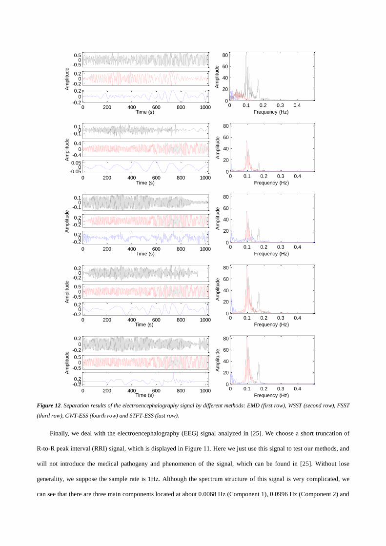
(third row), CWT-ESS (fourth row) and STFT-ESS (last row).
Finally, we deal with the electroencephalography (EEG) signal analyzed in [25]. We choose a short truncation of
R-to-R peak interval (RRI) signal, which is displayed in Figure 11. Here we just use this signal to test our methods, and
will not introduce the medical pathogeny and phenomenon of the signal, which can be found in [25]. Without lose
generality, we suppose the sample rate is 1Hz. Although the spectrum structure of this signal is very complicated, we
can see that there are three main components located at about 0.0068 Hz (Component 1), 0.0996 Hz (Component 2) and

0.1699 Hz (Component 3). By analyzing the TF distribution of this signal, we find that the three components are
separated. However, because of background noises and interferences, it is difficult to decompose this signal in
frequency domain or TF domain.
We use different methods to separate this signal, including EMD, WSST, FSST, CWT-ESS and STFT-ESS. Figure
12 shows the separation results with the left column showing the first three modes and the right column showing the
corresponding spectrums. Note that we use black color for Component 3, red for Component 2 and blue for Component
1. Because we have no prior information about the original signal, hence the RMSE cannot be applied to evaluate the
separation performance. Here we analyze the spectrum of the separation results. We say a method can separate this
signal well if the spectrums of the separation results are just corresponding to the three frequency components in Figure
11. EMD cannot separate Component 2 and Component 3 because of the mode mixing. All of WSST, FSST, CWT-ESS
and STFT-ESS can decompose this signal to its three main components. But by comparing the waveform and spectrum,
we find that Component 3 by WSST and Component 1 by FSST are not good. Both CWT-ESS and STFT-ESS enhance
the energy of the three components significantly. STFT-ESS has the best separation performance for Component 2 and
Component 3. CWT-ESS is the best among all these methods for the average separation performance of the three
components.
Conclusion
In this paper, we have introduced a new EMD-like method to separate multicomponent signal based on linear TF
analysis. Our method is adaptive and unsupervised. We have shown that the proposed method separates the models better
than EMD and the methods based on standard SST. In the sifting process of our method, we adjust the parameters for
CWT according to the spectrum of the signal adaptively. For multicomponent signals with IFs of components
intersecting each other, the methods of how to separate these signals both by our method and the standard SST will be the
subject for further study.
Acknowledgement
This work was supported in part by the National Natural Science Foundation of China (Grant No. 61201287) and
Simons Foundation Collaboration Grants for Mathematicians (Grant No. 353185).
Appendix
A. Proofs of Eq. (35)-(37).
From , , ,f s nW a b W a b W a b , we have

0
2
2
0
, ,
1( )
1lim lim ( )
1lim lim ,
f n
N
N tk N
N
nN t
k N
Var W a b Var W a b
tVar n t b dt
a a
k tVar n k t b t
a a
k tt
a a
where we know ( )n k t b is independent with ( )n j t b , if k j . Throughout this paper, we just let sampling
rate as 1 Hz, which means 1t , and consider the duration of f t is finite, namely 0,1, 1k N . Then we have
2
12 2
0
1,
N
f n n
k
kVar W a b C a
a a
, (A.2)
where 2
1
0
1N
k
kC a
a a
varies with scale a .
This shows (35).
Note that ,fVar W a b is irrelevant to the time translation b . By (36), for real and imaginary parts of CWT, we
have
, , ,
Im , Im , .
f s
f s
E e W a b e W a b
E W a b W a b
(A.3)
Analogously,
, , Im ,f f fVar W a b Var e W a b Var W a b
21, Im , .
2f f nVar e W a b Var W a b C a
Consider the Morlet’s wavelet, where is real. When 1b or 11 2 b , and 1 1 02 ( )a b ,
where 0ˆarg max ( )
, then 1 1,a b is the point with extreme value of the real part ,se W a b , with signal to
noise ratio
22
1 1 11 1
1 1 1 2
11 1
ˆ( ) 2 ( ),( , )
,
s
nf
A b a be W a br a b
C aVar e W a b
The signal-to-noise ratio is the same for the extrema of the imaginary part. Analogously, for ,fW a b , the signal to
noise ratio is defined by

22
1 1 11 1
2 1 1 2
11 1
ˆ( ) 2 ( ),( , )
2,
s
nf
A b a bW a br a b
C aVar W a b
These show Eq. (36) and Eq. (37).
B. Proof of Eq. (47).
For t given in (38), when , ˆ 0 for 0 . Thus for s t given by (46), when
( ) 0t c rt , we have
22 2 2 2 2
2
2 22 22 2 2
2 2
12 22 2 2
0
12 2 2
2 2 20 0
, ( )
( )
2
2 2
s
r xi cax cb a x abx b
i x
x xi ca rab x ra x cb rb
t b dtW a b s t
a a
s ax b x dx
Ak e e e e dx
A Ak e dx k e e
2 2 2
2 2
0 2 2 2
1
2, , , 0, , , ,
i ca rab x ra x cb rbdx
I a b e I a b
where 0 ,k c . According to the Fourier transform of a linearly-chirped Gaussian pulse [30],
2
02
0 4g ih t i t g ihe dt e
g ih
we have
2
2 22
2 2
4 1 22
02 2
, , ,2 1 2
ca rab
i rai cb i rbAI a b k e e
i ra
Let 2 2ca rab , and define ( )h by
22
22 2
1
21 2
( )ra
h e
. (B.4)
Then,
2 42
22 2
2 1 22
02 2
, , , ( )2 1 2
i ra
rai cb i rbAI a b k e e h
i ra
. (B.5)
Note that 2 21
2 0, , , 0e I a b
, Hence,

0 1
2 2 4
, , , , ( )2
1 2
s
AW a b I a b k h
ra
. (B.6)
Therefore, the ridge of ,sW a b is located at 2 2 0ca rab , namely 2 2
ac rb b
. The
bandwidths of ,sW a b and ( )h are the same, which is equal to
2
2 2
2
1 12
2h ra
. (B.7)
Hence, the support zone of ,sW a t is
2 2
2 2
h hab b
or
2 2
2 2
h hac rb c rb
.
This shows Eq. (47).
References
[1] N.E. Huang, Z. Shen, S.R. Long, M.C. Wu, H.H. Shih, Q. Zheng, N.-C. Yen, C.C. Tung, H.H. Liu, “The empirical mode
decomposition and the Hilbert spectrum for nonlinear and non-stationary time series analysis,” Proceeding of Royal Society A:
Mathematical, Physical and Engineering Science 454 (1998) 903-995.
[2] Q. Chen, N. Huang, S. Riemenschneider, Y. Xu, “A B-spline approach for empirical mode decompositions,” Advances in
Computational Mathematics 24 (2006) 171-195.
[3] C.K. Chui, M.D. van der Walt, “Signal analysis via instantaneous frequency estimation of signal components,” International
Journal on Geomathematics 6 (2015) 1-42.
[4] T. Oberlin, S. Meignen, V. Perrier, “An alternative formulation for the empirical mode decomposition,” IEEE Transactions on
Signal Processing 60 (2012) 2236-2246.
[5] L. Lin, Y. Wang,, H. Zhou, “Iterative filtering as an alternative algorithm for empirical mode decomposition,” Advances in
Adaptive Data Analysis 1 (2009) 543–560.
[6] F. Wu, L. Qu, “An improved method for restraining the end effect in empirical mode decomposition and its appplications to the
fault diagonosis of large ratating machinery,” Journal of Sound and Vibration 314 (2008) 586-602.
[7] G. Rilling, P. Flandrin, “One or two frequencies? The empirical mode decomposition answers,” IEEE Transations on Signal
Processin 56 (2008) 85-95.
[8] G. Rilling, P. Flandrin, “On the influence of sampling on the empirical mode decomposition,” ICASSP 2006, Toulouse, France,
vol. 3, pp. 444-447, May 2006.
[9] P. Flandrin, G. Rilling, P. Goncalves, “Empirical mode decomposition as a filter bank,” IEEE Signal Processing Letters 11
(2004) 112-114.

[10] L. Li, H. Ji, “Signal feature extraction based on improved EMD method,” Measurement 42 (2009) 796-803.
[11] Z. Wu, N. E. Huang, “Ensemble empirical mode decomposition: A noise-assisted data analysis method,” Advances in Adaptive
Data Analysis 1 (2009) 1-41.
[12] L. Cohen, “Time-frquency distributions-a review,” Proceedings of IEEE 77 (1979) 941-981.
[13] S. Qian, D. Chen, “Joint time-frequency analysis,” IEEE Signal Processing Magazine 16 (1999) 52-67.
[14] E. Sejdic, I. Djurovic, J. Jiang, “Time-frequency feature representation using enery concentration: An overview for recent
advances,” Digital Signal Processing 19 (2009) 153-183.
[15] A. Belouchrani, “Source separation and localization using time-frequency distribution: An overview,” IEEE Signal Processing
Magazine 30 (2013) 97-107.
[16] B. Boashash, “Time-frequency signal analysis and processing: A comprehensive reference,” Academic Press, 2015.
[17] F. Auger, P. Flandrin, “Improving the readability of time-frquency and time-scale representations by the reaassignment
method,” IEEE Transactions on Signal Processing 43 (1995) 1068-1089.
[18] I. Daubechies, S. Maes, “A nonlinear squeezing of the continuous wavelet transform based on auditory models,” Wavelet in
Medicine and Biology, pp. 527-546, CRC Press, 1996.
[19] I. Daubechies, J. Lu, H.-T. Wu, “Synchrosqueezed wavelet transforms: A empirical mode decomposition-like tool,” Applied
and Computational Harmonic Analysis 30 (2011) 243-261.
[20] C. Li, M. Liang, “A generalized synchrosqueezing transform for enhancing signal time-frequency representation,” Signal
Processing 92 (2012) 2264-2274.
[21] Q. Jiang, B. W. Suter, “Instantaneous frequency estimation based on synchrosqueezing wavelet transform,” Signal Processing
138 (2017) 167-181.
[22] I. Daubechies, Y. Wang, H.-T. Wu, “ConceFT: Concentration of frequency and time via a multitapered synchrosqueezed
transform,” Philosophical Transactions of The Royal Society A, vol. 374, July 2015.
[23] T. Oberlin, S. Meignen, V. Perrier, “The Fourier-based synchrosqueezing transform,” IEEE International Conference on
Acoustics, Speech and Signal Processing, pp. 315-319, May 2014, Florence, Italy.
[24] F. Auger, P. Flandrin, Y.-T. Lin, S. Mclaughlin, S. Meignen, T. Oberlin, H.-T. Wu, “Time-frequency reassignment and
synchrosqueezing : An overview,” IEEE Signal Processing Magazine 30 (2013) 32-41.
[25] T. Oberlin, S. Meignen, V. Perrier, “Second-order synchrosqueezing transform of inveritble reassignment? towards ideal
time-frequency representations,” IEEE Transactions on Signal Processing 63 (2015) 1335-1344.
[26] S. Wang, X. Chen, G. Cai, B. Chen, X. Li, Z. He, “Matching demodulation transform and synchrosqueezing in time-frequency
analysis,” IEEE Transactions on Signal Processing 62 (2014) 69-84.

[27] D. Iatsenko, P.-V.E. McClintock, A. Stefanovska, “Linear and synchrosqueezed time-frequency representations revisited:
Overview, standards of use, resolution, reconstruction, concentration, and alogorithms,” Digital Signal Processing 42 (2015)
1-26.
[28] J. Gilles, “Empirical wavelet transform,” IEEE Transactions on Signal Processing 61 (2013) 3999-4010.
[29] G. Thakur, E. Brevdo, N.-S. Fucar, H.-T. Wu, “The synchrosqueezing algorithm for time-varying spectral analysis: Robustness
properties and new paleoclimate applications,” Signal Processing 93 (2013) 1079-1094.
[30] D.J. Gibson, “Fourier transform of a linearly-chirped Gaussian pulse,” 2006, http://archive.physiker.us/files/physics/Chirped
PulseTransform.pdf.
[31] Y. Meyer , Wavelets and Operators, vol. 1, Cambridge University Press, 1993.
[32] I. Daubechies , Ten lectures on wavelets, SIAM, CBMS-NSF Regional Conference Series in Applied Mathematics, 1992.
[33] C. K. Chui, Q. Jiang, Applied Mathematics-Data Compression, Spectral Methods, Fourier Analysis, Wavelets and Applications,
Atlantis Press, Amsterdam, 2013.