an energy conservation algorithm for nonlinear dynamic

Hindawi Publishing CorporationJournal of Applied MathematicsVolume 2012, Article ID 453230, 18 pagesdoi:10.1155/2012/453230

Research ArticleAn Energy Conservation Algorithm forNonlinear Dynamic Equation

Jian Pang,1 Yu Du,2 Ping Hu,2, 3 Weidong Li,2, 3 and Z. D. Ma4

1 Changan Auto Global R&D Center, State Key Laboratory of Vehicle NVH and Safety Technology,Chongqing 401120, China

2 School of Automotive Engineering, Dalian University of Technology, Dalian 116024, China3 State Key Laboratory of Structural Analysis of Industrial Equipment, Dalian University of Technology,Dalian 116024, China

4 College of Engineering, University of Michigan, Ann Arbor, MI 48109-2133, USA

Correspondence should be addressed to Weidong Li, [email protected]

Received 14 July 2011; Revised 19 October 2011; Accepted 27 October 2011

Academic Editor: Ferenc Hartung

Copyright q 2012 Jian Pang et al. This is an open access article distributed under the CreativeCommons Attribution License, which permits unrestricted use, distribution, and reproduction inany medium, provided the original work is properly cited.

An energy conservation algorithm for numerically solving nonlinear multidegree-of-freedom(MDOF) dynamic equations is proposed. Firstly, by Taylor expansion and Duhamel integration,an integral iteration formula for numerically solving the nonlinear problems can be achieved.However, this formula still includes a parameter that is to be determined. Secondly, throughsome mathematical manipulations, the original dynamical equation can be further converted intoan energy conservation equation which can then be used to determine the unknown parameter.Finally, an accurate numerical result for the nonlinear problem is achieved by substituting thisparameter into the integral iteration formula. Several examples are used to compare the currentmethod with the well-known Runge-Kutta method. They all show that the energy conservationalgorithm introduced in this study can eliminate algorithm damping inherent in the Runge-Kuttaalgorithm and also has better stability for large integral steps.

1. Introduction

Numerical stability and algorithmic damping have been long recognized as two importantaspects that need to be carefully handled in time integration algorithms for solving dynamicproblems. Indeed, many works have been done in this area. For instance, to improve thestability, the Generalized-α method of Chung and Hulbert [1], the HHT-α method of Hilberet al. [2], and the WBZ-α method of Wood et al. [3] all demonstrate very good dissipationproperty either at low-frequency or high-frequency ranges. In references [4–8], Fung presentsa series of time-step algorithms that are based on different mathematical and mechanicalprinciples and can be used to deal with linear dynamical problems. Recent works on

2 Journal of Applied Mathematics

numerical methods have been focusing on modeling long-term qualitative properties andstabilities in the numerical solutions of nonlinear dynamic problems. In the past, the featureof the energy conservation of a system has been widely used in various numerical integrationmethods to achieve satisfactory results. Since the property of exact energy conservationenables the numerical scheme to be stable without resorting to high-frequency numericaldissipation [9], the feature of the energy conservation appears particularly attractive innumerically solving nonlinear dynamic systems. Consequently, much effort has gone intothe development of energy conserving time-stepping schemes. By adding an additionalconstraint through the energy conservation equation between adjacent time steps, Buiproposed a modified Newmark family for nonlinear dynamic analysis [10]. Similar worksare also reported by LaBudde and Greenspan [11], Hughes et al. [12], Greespan [13], Simoand Tarnow [14], Simo et al. [15], Greenspan [16], and Fung and Chow [17]. Interestingly,all works cited above derived their algorithms starting with the finite difference method, andmost of them were based on Hamilton’s canonical equations of motion.

Though energy conservative methods have showed some advantages, they also mightsuffer from some drawbacks in practical applications. In an attempt to obtain a stable large-step integration, Simo and Gonzalez [9] used the energy-momentum algorithm, which wasobtained from the modification of midpoint scheme. By doing this, they risked to wronglyapproximate slowly varying solution quantities in highly oscillatory systems, which wasespecially significant when fast and low modes are tightly coupled [18]. Moreover, with theaddition of the constraint on the energy conservation, one has an overdetermined system thatthe exact solution has to satisfy. However, once the system is discretized and approximated inorder to solve it numerically, the overdetermined systemmay not have a solution anymore. Inother words, difficulties may occur in the multidimensional root finding of the correspondingnonlinear system of equations [19].

In this paper, the authors proposed a time integration formula and scheme whichcan maintain the system energy conservation constraint automatically. However, thismethod is also different from the energy conservative methods developed previously in thefollowing four aspects. Firstly, the solution of the nonlinear dynamic equation was presentedanalytically by Duhamel integral in the current method. Secondly, the current methodused the Taylor expansion to approximate the exact solution of the nonlinear equation.During this process, an undetermined parameter was introduced. Thirdly, substituting theapproximate solution into the analytical solution, an iterative formula with the undeterminedparameter was derived. Finally, the energy conservation equation was established andthe undetermined parameter was obtained. In practice, how to introduce and obtain theundetermined parameter should be carefully considered case by case, especially when theright hand term of the nonlinear equation includes functions of velocity and time. Anothermerit of the current algorithm was that it behaved very stable under large time steps.Comparisons with the Rounge-Kutta method showed that the proposed method had muchbetter stabilities in solving different types of nonlinear equations.

The remainder of this paper is arranged as follows. In Section 2, a detailed processof deriving the integral iteration formula is presented. In the iteration formula, we willshow that how an undetermined parameter is introduced into the formula. In Section 3,the energy conservation equation is established for obtaining the algebraic expressionof the undetermined parameter. Section 4 focuses on the calculation of the multinomialinterpolation used in Section 2. Section 5 shows some representative numerical exampleswhich compare the current method with the popular Runge-Kutta method in terms of

Journal of Applied Mathematics 3

algorithmic damping and stability. Finally, some discussions and conclusions are given inSection 6.

2. Derivation of the Integral Iteration Formula

Step-by-step time-integration algorithms are commonly used to solve dynamic equationswhich mostly come from actual engineering problems. By spatial discretization using thefinite element method, a nonlinear system may be represented by a second order nonlinearordinary differential equation as

Mx +Kx = f(x, x, t), (2.1)

where M, K are n-by-n constant mass and stiffness matrices, respectively. x, x, x, f arevectors with rank n representing the displacement, velocity, and acceleration, respectively.t is time. The right hand term in (2.1), f(x, x, t), is the force vector that includes all externalforces such as the damping forces and the nonlinear forces. Using the matrix decomposition,the mass matrix M can be expressed as

M = L · LT M−1 = L−T · L−1. (2.2)

Substituting (2.2) into (2.1) and multiplying by L−1, we can obtain

LT x + L−1KL−T · LTx = L−1f. (2.3)

Knowing that L, L−1, LT , L−T are all constant matrices, a variable substitution can beexecuted as

y = LTx, y = LT x, y = LT x. (2.4)

Substituting (2.4) into (2.3), a new dynamic systemwhich is equivalent to the original systemcan be obtained as

y +Ky = F(t), F(t) = L−1f(t), K = L−1KL−T . (2.5)

Let

K = K0 +D, (2.6)

where D is a diagonal matrix and its diagonal elements are the diagonal elements of matrixK. K0 is a matrix whose diagonal elements are zero, and other elements are equal to those inK. Note that Dii ≥ 0 forMwhich is a positive definite matrix and K is a semipositive definitematrix. Let

Dii = d2i . (2.7)


Then (2.5) can be rewritten as

y +Dy = F(t) −K0y. (2.8)

The separate form of the above matrix equation can be expressed as follows:

yi + d2i yi = Fi(t) − ki

0y, i = 1, 2, . . . , n, (2.9)

where ki0 is the ith row of the matrixK0. From (2.9), it is easy to see that the analytical solution

of the displacement and the velocity can be obtained by the Duhamel integral as

yi(t) = yi(tk) cosdi(t − tk) + yi(tk)sindi(t − tk)

di

+1di

∫ t

tk

Fi(ς) sindi(t − ς)dς − 1di

∫ t

tk

ki0y(ς) sindi(t − ς)dς,

(2.10)

yi(t) = −yi(tk)di sindi(t − tk) + yi(tk) cosdi(t − tk)

+∫ t

tk

Fi(ς) cosdi(t − ς)dς −∫ t

tk

ki0y(ς) cosdi(t − ς)dς.

(2.11)

In order to derive the time integral formula, let t = tk + τ in (2.10) and (2.11), where τis the integral time step, then we have

yi(tk + τ) = yi(tk) cosdiτ + yi(tk)sindiτ

di+

1di

∫ tk+τ

tk

Fi(ς) sindi(tk + τ − ς)dς

− 1di

∫ tk+τ

tk

ki0y(ς) sindi(tk + τ − ς)dς,

(2.12)

yi(tk + τ) = −yi(tk)di sindiτ + yi(tk) cosdiτ +∫ tk+τ

tk

Fi(ς) cosdi(tk + τ − ς)dς

−∫ tk+τ

tk

ki0y(ς) cosdi(tk + τ − ς)dς.

(2.13)

Inspecting (2.12) and (2.13), it can be found that there are still some unknownparameters that need to be identified before the time integral formula can be carried outnumerically. They are the right hand side terms consisting of the undetermined variablesy(t) and Fi(t). The latter one may also be a function of y(t) and y(t). To proceed, the Taylorexpansion formula is used to expand y(t) on the interval (tk ≤ t ≤ tk + τ) as

y(t) = y(tk) + (t − tk)y(tk) +(t − tk)2

2y(tk) +

(t − tk)3

6a. (2.14)

In (2.14), y(t) is expanded to the third order term following exactly the Taylorexpansion process, while in calculating the fourth order term, a new variable vector a is


introduced. It should be pointed out that although the Taylor expansion is an approximationto the original variable y(t), (2.14) is still an exact expression of the variable y(t). Thisis because the last term in (2.14) which includes the newly introduced vector a can beinterpreted to compensate for the difference between y(t) and the summation of the first threeterms in (2.14). In order to express the vector a by the variable y(t), let y1 = y(t = tk + τ), y0 =y(t = tk). From (2.14), it can be obtained that

a =6τ3

(y1 − y0 − τ y0 − τ2

2y0

),

y(t) = N1(t)y0 +N2(t)y0 +N3(t)y0 +N4(t)y1,

(2.15)

where:

N1(t) = 1 − (t − tk)3

τ3, N2(t) = t − tk − (t − tk)3

τ2,

N3(t) =(t − tk)2

2− (t − tk)3

2τ, N4(t) = β(t − tk)3(t − tk − τ) +

(t − tk)3

τ3,

(2.16)

where an undetermined parameter β has been introduced inN4(t) to regulate the stability ofthe algorithm andwill be determined by the energy conservation equation in the next section.By t = tk, t = tk + τ in (2.14), we can obtain

y(tk) = y0, y(tk) = y0, y(tk) = y0, y(tk + τ) = y1. (2.17)

By means of multinomial interpolation, f(t) (tk ≤ t ≤ tk + τ) can be written as

f(t) = r0 + (t − tk)r1 + (t − tk)2r2 + (t − tk)3r3 + o((t − tk)4

). (2.18)

Here we use the third order interpolation, and generally one can choose the orderof interpolation discretionarily based on solely the algorithm accuracy order that is needed.Different interpolation order will lead to different integration formulas. Now, we will derivethe integration formulas first, and the discussion of the interpolation will be addressedat Section 4. Using (2.5) and (2.14), the last two terms of the right hand of (2.11) can beexpressed separately as

1di

∫ tk+τ

tk

ki0y(ς) sindi(tk + τ − ς)dς = αi

0ki0y0 + αi

1ki0y0 + αi

2ki0y0 + αi

3ki0y1,

1di

∫ tk+τ

tk

L−1i f(ς) sindi(tk + τ − ς)dς = γi0L

−1i r0 + γi1L

−1i r1 + γi2L

−1i r2 + γi3L

−1i r3,

(2.19)


where αik, γ ik, k = 0, 1, 2, 3 are scalar and can be obtained by follow polynomials

αi0 = −

(6 sindiτ + d3

i τ3 cosdiτ − 6diτ

)d5i τ

3,

αi1 =

(6diτ − d2

i τ2 sindiτ − 6 sindiτ

)d5i τ

2,

αi2 =

(2diτ − 3 sindiτ + diτ cosdiτ)d5i τ

,

αi3 =

(6 sindiτ + d3

i τ3 − 6diτ

)d5i τ

3− β(d2i τ

2 − 4 + 4 cosdiτ + diτ sindiτ)

d6i τ

4,

γ i0 =(1 − cosdiτ)

d2i

,

γ i1 =(diτ − sindiτ)

d3i

,

γ i2 =

(d2i τ

2 − 2 + 2 cosdiτ)

d4i

,

γ i3 =

(d3i τ

3 − 6diτ + 6 sindiτ)

d5i

.

(2.20)

Substituting (2.20) into (2.12), we have

yi(tk + τ) = yi(tk) cosdiτ + yi(tk)sindiτ

di+ γi0L

−1i r0 + γi1L

−1i r1 + γi2L

−1i r2

+ γi3L−1i r3 −

(αi0k

i0y0 + αi

1ki0y0 + αi

2ki0y0 + αi

3ki0y1)

(i = 1, 2, . . . , n).(2.21)

Knowing that y1 = y(t = tk + τ), so we can write the above equation in a matrix form:

y1 = U0y0 +U1y0 + γ0L−1r0 + γ1L

−1r1 + γ2L−1r2

+γ3L−1r3 − α0K0y0 − α1K0y0 − α2K0y0 − α3K0y1,

(2.22)

where U0, U1, αk, γk (k = 0, 1, 2, 3) are diagonal matrices and their diagonal elements arecosdiτ , sindiτ/di, αi

k, γi

k(i = 1, 2, . . . , n, k = 0, 1, 2, 3), respectively. From (2.22), the iterative

solution y1 can be expressed as

(I + α3K0)y1 = (U0 − α0K0)y0 + (U1 − α1K0)y0 − α2K0y0 + γ0L−1r0

+ γ1L−1r1 + γ2L

−1r2 + γ3L−1r3.

(2.23)


Multiplying (2.23) by Lα−13 , we have

L(α−13 +K0

)y1 = Lα−1

3 (U0 − α0K0)y0 + Lα−13 (U1 − α1K0)y0

− Lα−13 α2K0y0 + Lα−1

3 γ0L−1r0 + γ1L

−1r1 + γ2L−1r2 + γ3L

−1r3.(2.24)

Note that K0 is a matrix whose diagonal elements are zero, and other elements areequal to those in K and αk is a diagonal matrix, so L(α−1

3 + K0) is a symmetrical matrix. Theleft hand side of (2.24) can be written as

L(α−13 +K0

)LTL−Ty1 =

(Lα−1

3 LT + LK0LT)L−Ty1. (2.25)

From (2.5) and (2.6), we have

LK0LT = L ·(K −D

)· LT = L · L−1KL−T · LT − LDLT = K − LDLT . (2.26)

From (2.3) and (2.26), the left hand of (2.24) can be written as

L(α−13 +K0

)y1 =

[K + L

(α−13 −D

)LT]· x1. (2.27)

All the terms in the right hand side of (2.24) can be expressed separately as

Lα−13 (U0 − α0K0)y0 =

[L(α−13 U0 + α−1

3 α0D)LT − Lα−1

3 α0L−1K]· x0,

Lα−13 (U1 − α1K0)y0 =

[L(α−13 U1 + α−1


3 α1L−1K]· x0,

Lα−13 α2K0y0 = Lα−1

3 α2L−1LK0LTL−T y0 = Lα−13 α2L−1

(K − LDLT

)· x0.

(2.28)

After substituting proper variables, the iteration formula in terms of the original variablescan be expressed as

[K + L

(α−13 −D

)LT]· x1

=[L(α−13 U0 + α−1


3 α0L−1K]· x0

+[L(α−13 U1 + α−1


3 α1L−1K]· x0 − Lα−1

3 α2L−1(K − LDLT

)· x0

+ Lα−13 γ0L

−1r0 + Lα−13 γ1L

−1r1 + Lα−13 γ2L

−1r2 + Lα−13 γ3L

−1r3.

(2.29)


In (2.29), there is a term consisting of a double derivative. According to (2.3), theterm with the double derivative x0 can be replaced by −L−TL−1Kx0 + L−TL−1f0. Finally, thedisplacement iteration formula can be obtained as

[K + L

(α−13 −D

)LT]· x1

= L ·[(

α−13 U0 + α−1

3 α0D)LT − α−1

3 α0L−1K + α−13 α2L−1

(K − LDLT

)L−TL−1K

]· x0

+ L ·[(

α−13 U1 + α−1

3 α1D)LT − α−1

3 α1L−1K]· x0

+ L ·[α−13 γ0L

−1 − α−13 α2L−1

(K − LDLT

)· L−TL−1

]r0

+ Lα−13 γ1L

−1r1 + Lα−13 γ2L

−1r2 + Lα−13 γ3L

−1r3.

(2.30)

Substituting (2.14) and (2.15) into (2.13) and through some mathematical manipula-tions, the velocity iteration formula can be obtained as

x1 = Rτx1 + R0x0 + R1x0 + L−T[η0L

−1 −(c2L−1K − c2DLT

)L−TL−1

]r0

+ L−Tη1L−1r1 + L−Tη2L

−1r2 + L−Tη3L−1r3,

(2.31)

where η0, η1, η2, η3 are diagonal matrices with diagonal elements ηi0, η

i1, η

i2, η

i3, respectively.

cm is also a diagonal matrix and its diagonal elements are cim (m = 0, 1, 2, 3). Every term inthe right hand side of (2.31) is given as bellow:

R0 = L−T[(

V0LT + c0DLT − c0L−1K)+ c2L−1K − c2DLT

)L−TL−1 ·K,

R1 = L−T(V1LT + c1DLT − c1L−1K

),

Rτ = −L−Tc3(L−1K −DLT

),

ci0 =

(d3i τ

3 sindiτ − 6 cosdiτ − 3d2i τ

2 + 6)

d4i τ

3,

ci1 = −(d2i τ

2 cosdiτ + 6 cosdiτ + 2d2i τ

2 − 6]

d4i τ

2,

ci2 = − (1/2)(2diτ sindiτ + 6 cosdiτ + d2

i τ2 − 6

)d4i τ

,

ci3 =

(6 cosdiτ + 3d2

i τ2 − 6

)d4i τ

3− β(6diτ cosdiτ − 24 sindiτ − d2

i τ2 + 18

)d5i τ

4,

ηi0 =

sindiτ

diηi1 =

1 − cosdiτ

d2i

ηi2 =

2diτ − 2 sindiτ

d3i

,

ηi3 =∫ tk+τ

tk

(ς − tk)3 cosdi(tk + τ − ς)dς,

(2.32)

where V0, V1 are diagonal matrices with diagonal elements −di sindiτ , cosdiτ , respectively.


3. Energy Conservation Equation

One reason of expressing the dynamic equation in the form of (2.1) is to establish the energyconservation equation more conveniently and more directly. The following steps illustratethe construction of the energy conservation equation. Multiplying xT to both sides of (2.1),we have

xTMx + xTKx = xT f(x, x, t). (3.1)

Integrating (2.32) from tk to tk+1, we can obtain

∫ tk+1

tk

xTMxdt +∫ tk+1

tk

xTKxdt =∫ tk+1

tk

xT fdt k = 0, 1, 2, 3, . . . , (3.2)

namely,

12xTMx

∣∣∣∣tk+1

tk

+12xTKx

∣∣∣∣tk+1

tk

=∫ tk+1

tk

xT fdt k = 0, 1, 2, 3, . . . . (3.3)

Simplifying (3.3), we can obtain an energy conservation equation between tk andtk+1 as follows:

Tk+1 − Tk + Vk+1 − Vk =∫ tk+1

tk

xT fdt k = 0, 1, 2, 3, . . . , (3.4)

where

Tk+1 =12xTk+1Mxk+1, Tk =

12xTkMxk, V k+1 =

12xTk+1Kxk+1, V k =

12xTkKxk. (3.5)

Substituting (2.30) and (2.31) into the left hand side of (3.4), a polynomial of theundermined parameter β can be easily achieved. For the right hand side of (3.4), the integralterm can be firstly decomposed into two parts as follows:

f1 =∫ tk+1

tk

xTq1(x)dt, f2 =∫ tk+1

tk

xTq2(x, t)dt, (3.6)

where the term f1 is an integral of an autonomous system and can be integrated easily.The x(t) in term f2 can be expressed as a polynomial of time using the relationship in(2.4) and taking the derivative of (2.15) with respect to time. Two predictive methods arerecommended for determining the unknown term y1 in (2.15). One is to let y1 = y0 + y0τ andthe other is to let β = 1 in (2.23).

Then through (3.5), an algebraic equation with an undetermined parameter β can beestablished and β can be numerically obtained by the Newton iteration method or otheralgebraic methods. Finally, substituting β into (2.30) and (2.31), a numerical result can thenbe achieved.


4. Calculations of the Interpolation

Before giving some numerical examples, choosing the proper interpolation form of (2.18)must be discussed because it will affect the accuracy and stability of the proposedalgorithm. In the current study, the authors use the Hermite interpolation to approximatethe r1, r2, r3, r4 in (2.18), that is,

⎧⎪⎪⎪⎪⎪⎪⎪⎪⎨⎪⎪⎪⎪⎪⎪⎪⎪⎩

ri0

ri1

ri2

ri3

⎫⎪⎪⎪⎪⎪⎪⎪⎪⎬⎪⎪⎪⎪⎪⎪⎪⎪⎭

=

⎡⎢⎢⎢⎢⎢⎢⎢⎢⎢⎢⎢⎢⎢⎣

1 0 0 0

− 1τ

01τ

0

− 3τ2

− 2τ

3τ2

− 1τ

2τ3

1τ2

− 2τ3

1τ2

⎤⎥⎥⎥⎥⎥⎥⎥⎥⎥⎥⎥⎥⎥⎦

·

⎧⎪⎪⎪⎪⎪⎪⎨⎪⎪⎪⎪⎪⎪⎩

fi(0, xi(0), xi(0))

f ′i(0, xi(0), xi(0))

fi(t, xi(τ), xi(τ))

f ′i(t, xi(τ), xi(τ))

⎫⎪⎪⎪⎪⎪⎪⎬⎪⎪⎪⎪⎪⎪⎭. (4.1)

It should be noted that there are unknowns in the right hand term of (4.1) which arexi(τ), xi(τ). The prediction of the two unknowns is shown below. For example, we can let

xi(τ) = xi(0) + xi(0) · τ,xi(τ) = xi(0) + xi(0) · τ.

(4.2)

Then at every iteration of (3.4), the parameter β can be updated. Submitting β into(2.30) and (2.31), a new prediction of the displacement and velocity can therefore be obtained.

5. Numerical Examples

In this section we give some numerical examples to verify the effectiveness of the proposedalgorithm, in particular, the advantage in stability of the proposed algorithm. Since (2.14)is a fourth order Taylor expansion, the energy conservation algorithm has fourth orderaccuracy. So we choose the Rounge-Kutta method as a numerical comparison. The numericalresults show the advantages of the proposed energy conservation algorithm in terms ofits integration stability and the ability to eliminate the algorithm damping inherent in theRounge-Kutta method.

5.1. The Oscillation of a Nonlinear Simple Pendulum

The dynamic equation of a nonlinear single pendulum without damping can be written as

x +ω20 sinx = 0, ω2

0 = 1.0, x(0) = 1.57, (5.1)

where x denotes the angular displacement. The numerical solutions are shown in Figure 1.From the figure we can see that the proposed energy conservation method (ECM) can keepthe numerical stability and have no computing damping under large-step comparingwith theRounge-Kutta (RK)method. The numerical result of parameter β is shown in Figure 2. Table 1


0 10 20 30 40 50 60

0

0.5

1

1.5

2

RK ts = 0.001RK ts = 1ECM ts = 1

−2

−1.5

−1

−0.5

x

t

Figure 1: Angular Displacement comparison between the proposed energy conservation method (ECM)and the RK method.

0 10 20 30 40 50 600.998

0.999

1

1.001

1.002

1.003

1.004

t

β

Figure 2: Value of parameter β (time step = 1.0 s).

gives the comparison of the computing efficiency. The efficiency of the proposed method isnot as good as the RK method due to the iteration of parameter β and the time needed tocompute the associated matrices. Figure 3 gives the error analysis between the ECM and theRK under time step 1.0 s.

5.2. The Unforced Linear Vibration of the Cuboid Rigid Body with Two DOF

The structural diagram of the system is shown in Figure 4. The mass of the rigid body is mand the length of the hemline is a. The center of mass is collocated at the geometry center


ts = 1

10−3

10−2

10−1

100

101

100 101 102

t

abs(

del

t(x))

Figure 3: The log-log plot of the error between the ECM and RK.

Table 1: Comparison of computing efficiency.

CPU Memory Integrations Steps End time Time elapsed

RK Intel core2 2.26G 2G 500000 0.001 s 500 s 5.736 sECM Intel core2 2.26G 2G 500 1.0 s 500 s 1m7.123 s

(point C). The mass moment of inertia around the center of mass is J and the stiffness ofthe spring is k. The deformations of the two springs are x1, x2. The displacement in verticaldirection of the center of mass is xc. The angular displacement of the rigid body about themass center is φ. Using the above parameters, the equation of motion of the system can bewritten as

⎡⎢⎢⎣m

4+

J

a2

m

4− J

a2

m

4− J

a2

m

4+

J

a2

⎤⎥⎥⎦{x1

x2

}+[k 00 k

]{x1

x2

}={00

}. (5.2)

Let m = 8, a = 1, k = 2, J = 1, x1 = 1, and x2 = −1. Figures 5 and 6 compare thedisplacement (x1) and velocity (x2-dot) results predicted by the proposed method and theRK method. It can be seen that even with a big time step 1.0 s, the proposed method still hasan accurate numerical solution but the RK method does not. Table 2 gives the comparisonof the computing efficiency. Again, the efficiency of the proposed method is lower than thatof the RK method in calculating these two degrees of freedom problem. Furthermore, it isnoticed that the RK method almost keeps the same efficiency in Sections 5.1 and 5.2.

Figure 7 gives the error analysis between the ECM and the RK under time step 1.0 s.As Figure 7 already shows that the accuracy of the ECM is almost same as the result of RKwith a 0.001 time step, the comparison does not use the RK with a small time step.


φ xc

Jc

m

x1

k k

x2

a

Figure 4: Structural diagram of the cuboid rigid body.

0 10 20 30 40 50 60

0

0.2

0.4

0.6

0.8

1

RK time step = 1ECM time step = 1RK time step = 0.001

−1

−0.8

−0.6

−0.4

−0.2

x1

t

Figure 5: Comparison of displacement.

5.3. The Unforced Nonlinear Oscillation of a Spring Pendulum withTwo DOF

The dynamic equation of the spring pendulum can be written as

x1 + 2c1x1 +ω21x1 − b1x1x2 = 0,

x2 + 2c2x2 +ω22x2 − b2x

21 = 0.

(5.3)

Figures 8 and 9 show the numerical solution under different damping. Parameters andinitial condition are given as follows:

ω1 = 1.0, ω2 = 1.5, b1 = b2 = 1.0, x1 = x2 = 0.1, x1 = x2 = 0.0. (5.4)


0 10 20 30 40 50 60

0

0.2

0.4

0.6

0.8

1

RK time step = 1ECM time step = 1RK time step = 0.001

−1

−0.8

−0.6

−0.4

−0.2dx

2

t

Figure 6: Comparison of velocity.

10−4

10−3

10−2

10−1

100

100 101 102

t

abs(

del

t(x))

Figure 7: The log-log plot of the error between the ECM and RK with time step 1.0 s.

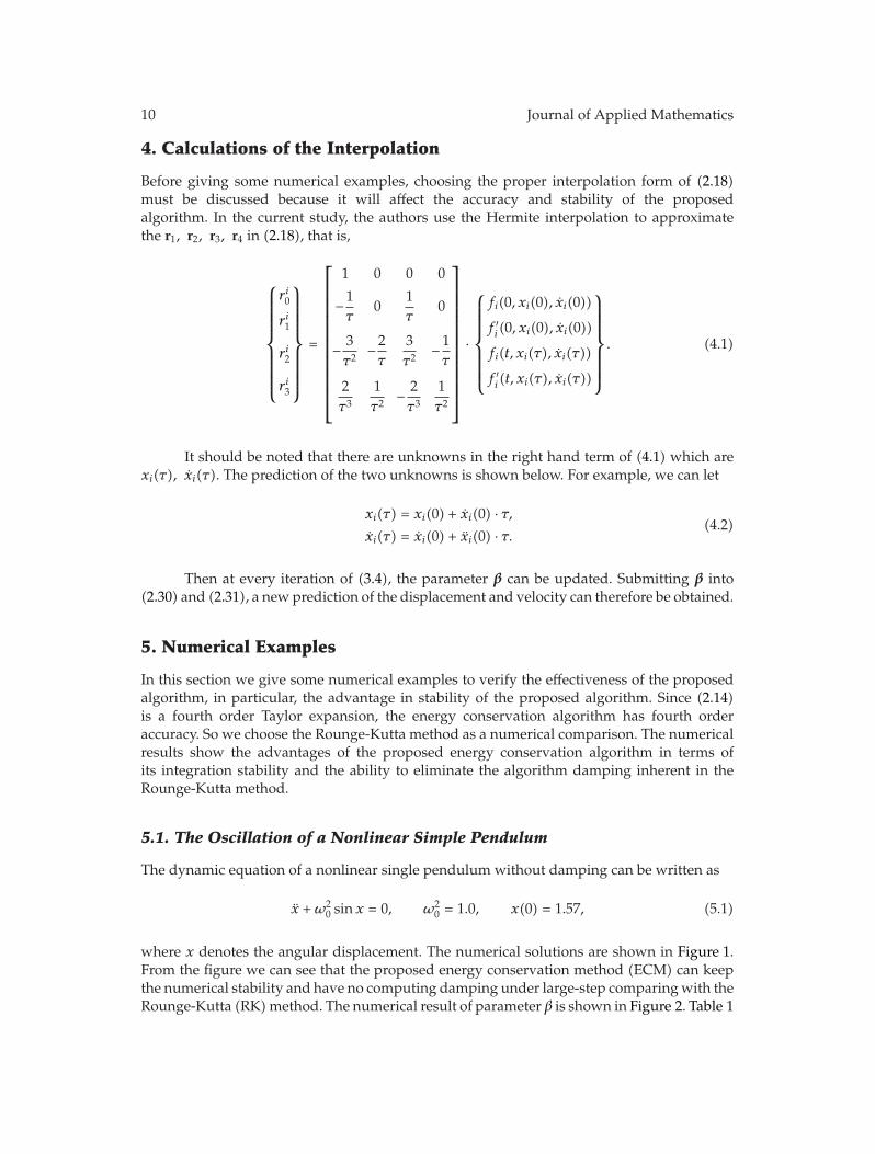
Figure 10 shows the comparison of the numerical results between ECM and RKmethods under large time steps. It is obvious that the proposed method can eliminatealgorithm damping better and provides better stability than the RK scheme. Parameters andinitial conditions used in the calculation are as follows:

c1 = c2 = 0.0, ω1 = 1.0, ω2 = 1.5,

b1 = b2 = 1.0, x1 = x2 = 0.1, x1 = x2 = 0.0.(5.5)


0 10 20 30 40 50 60 70

0

0.02

0.04

0.06

0.08

0.1

−0.1

−0.08

−0.06

−0.04

−0.02x

1

t

ECM c = 0 ts = 0.1RK c = 0 ts = 0.001ECM c = 1 ts = 0.1

RK c = 1 ts = 0.001ECM c = 10 ts = 0.1RK c = 10 ts = 0.001

Figure 8: Displacement trajectory.

0 10 20 30 40 50 60 70

0

0.05

0.1

0.15

−0.2

−0.15

−0.1

−0.05

t

dx

2

ECM c = 0 ts = 0.1RK c = 0 ts = 0.001ECM c = 1 ts = 0.1

RK c = 1 ts = 0.001ECM c = 10 ts = 0.1RK c = 10 ts = 0.001

Figure 9: Velocity trajectory.


CPU Memory Integrations Steps End time Time elapsed

RK Intel core2 2.26G 2G 500000 0.001 s 500 s 5.849 sECM Intel core2 2.26G 2G 500 1.0 s 500 s 1m 11.741 s


0 10 20 30 40 50 60

0

0.02

0.04

0.06

0.08

0.1

−0.1

−0.08

−0.06

−0.04

−0.02x

1

t

RK c = 0 ts = 0.001RK c = 0 ts = 1ECM c = 0 ts = 1


450 460 470 480 490 500 510

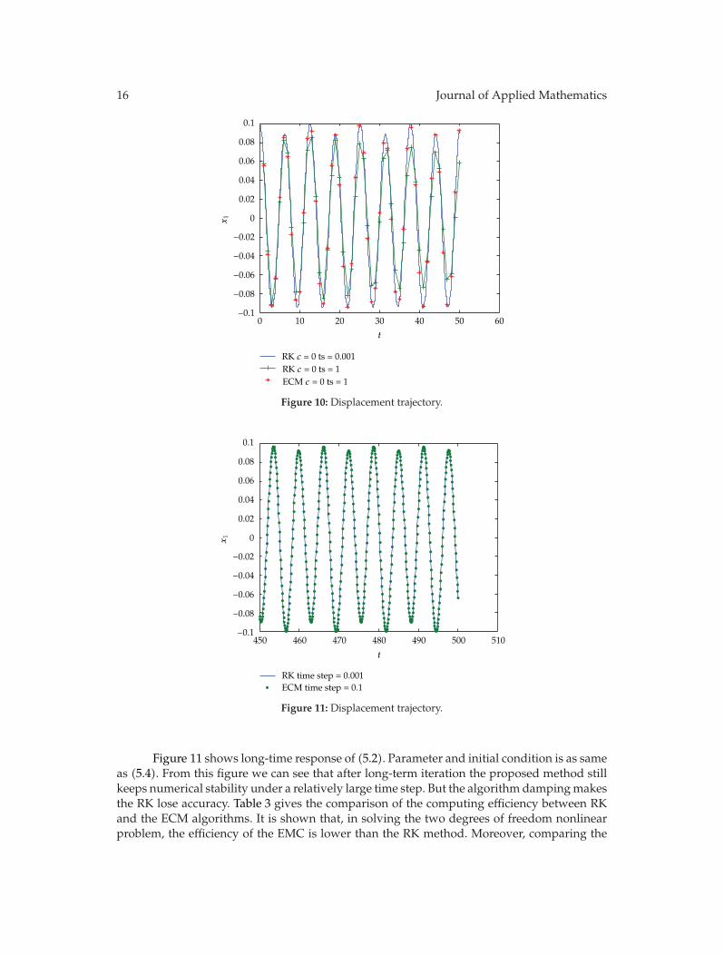
RK time step = 0.001ECM time step = 0.1

0

0.02

0.04

0.06

0.08

0.1

−0.1

−0.08

−0.06

−0.04

−0.02

x1

t


Figure 11 shows long-time response of (5.2). Parameter and initial condition is as sameas (5.4). From this figure we can see that after long-term iteration the proposed method stillkeeps numerical stability under a relatively large time step. But the algorithm dampingmakesthe RK lose accuracy. Table 3 gives the comparison of the computing efficiency between RKand the ECM algorithms. It is shown that, in solving the two degrees of freedom nonlinearproblem, the efficiency of the EMC is lower than the RK method. Moreover, comparing the


10−4

10−3

10−2

10−1

100 101 102

t

abs(d

elt(x

1))

c = 0 time step = 1

Figure 12: The log-log plot of the error between the ECM and RK.


CPU Memory Integrations Steps End time Time consuming

RK Intel core2 2.26G 2G 500000 0.001 s 500 s 6.655 sECM Intel core2 2.26G 2G 500 1.0 s 500 s 4m 18.263 s

elapsed time by the ECM in Table 2 and Table 3, it also can be seen that the computationefficiency of the ECM is worse for calculating nonlinear problems than for linear problems.Figure 12 shows the error analysis between the ECM and the RK under time step 1.0 s.

6. Conclusion

(1) The energy conservation algorithm has the advantage in stability and time step comparedwith some numerical means because the numerical solution has been corrected by the energyconservation equation.

(2) All examples have shown that the energy conservation method can eliminatealgorithm damping. It is also an effective means for calculating the long-term characteristicsof nonlinear dynamic systems.

(3) The proposed method conserves the angular momentum automatically. Althoughthe efficiency of the energy conservation method is not as good as the RK algorithm as well assome other numerical methods discussed in the literature, the integration step is large enoughto implement long-term integration with good numerical stability.

(4) The reason of the low efficiency of the proposed method is because the iterationsneed to calculate the parameter β and the time consumed in matrix computing needed by thealgorithm. The efficiency of the EMC is lower in dealing with nonlinear problems comparedwith linear problems.


Acknowledgments

This workwas funded by the “973”National Basic Research Project of China (no. Q10110919),Key Project of the National Natural Science Foundation of China (no. 10932003), “863” Projectof China (no. 2009AA04Z101), and “973” National Basic Research Project of China (no.2010CB832700). These supports are gratefully acknowledged. Many thanks are due to thereviewers for their valuable comments.

References

[1] J. Chung and G. M. Hulbert, “A time integration algorithm for structural dynamics with improvednumerical dissipation: the generalized- α method,” Journal of Applied Mechanics, vol. 60, no. 2, pp.371–375, 1993.

[2] H. M. Hilber, T. J. R. Huge, and R. L. Taylor, “Improved numerical dissipation for time integrationalgorithms in structural dynamics,” Earthquake Engineering and Structural Dynamics, vol. 5, pp. 283–292, 1977.

[3] W. L.Wood, M. Bossak, and O. C. Zienkiewicz, “An alphamodification of Newmark’s method,” Inter-national Journal for Numerical Methods in Engineering, vol. 15, pp. 1562–1566, 1981.

[4] T. C. Fung, “Unconditionally stable time-step-integration algorithms based on Hamilton’s principle,”AIAA Journal, vol. 38, no. 8, pp. 1443–1464, 2000.

[5] T. C. Fung, “On the equivalence of the time domain differential quadrature method and the dissipa-tive Runge-Kutta collocation method,” International Journal for Numerical Methods in Engineering, vol.53, no. 2, pp. 409–431, 2002.

[6] T. C. Fung, “Construction of higher-order accurate time-step integration algorithms by equal-orderpolynomial projection,” Journal of Vibration and Control, vol. 11, no. 1, pp. 19–49, 2005.

[7] T. C. Fung, “Bi-discontinuous time step integration algorithms-Part 2: second-order equations,”Computer Methods in Applied Mechanics and Engineering, vol. 192, no. 3-4, pp. 351–374, 2003.

[8] T. C. Fung and Z. L. Chen, “Krylov precise time-step integration method,” International Journal forNumerical Methods in Engineering, vol. 68, no. 11, pp. 1115–1136, 2006.

[9] J. C. Simo and O. Gonzalez, “Assessment of energy-momentum and sympletic schemes for stiffdynamic systems,” in Proceedings of the ASME Winter Annual Meeting, New Orleans, La, USA,December 1993.

[10] Q. V. Bui, “Modified Newmark family for non-linear dynamic analysis,” International Journal for Nu-merical Methods in Engineering, vol. 61, no. 9, pp. 1390–1420, 2004.

[11] R. A. LaBudde and D. Greenspan, “Energy and momentum conserving methods of arbitrary orderfor the mumerical integration of equations of motion, II. Motion of a system of particles,” NumerischeMathematik, vol. 26, no. 1, pp. 1–16, 1976.

[12] T. J. R. Hughes, T. K. Caughey, and W. K. Liu, “Finite-element methods for nonlinear elastodynamicswhich conserve energy,” Journal of Applied Mechanics, vol. 45, no. 2, pp. 366–370, 1978.

[13] D. Greenspan, “Conservative numerical methods for x = f(x),” Journal of Computational Physics, vol.56, no. 1, pp. 28–41, 1984.

[14] J. C. Simo and N. Tarnow, “The discrete energy-momentum method. Conserving algorithms for non-linear elastodynamics,” Journal of Applied Mathematics and Physics (ZAMP), vol. 43, no. 5, pp. 757–792,1992.

[15] J. C. Simo, N. Tarnow, and K. K. Wong, “Exact energy-momentum conserving algorithms and sym-plectic schemes for nonlinear dynamics,” Computer Methods in Applied Mechanics and Engineering, vol.100, no. 1, pp. 63–116, 1992.

[16] D. Greenspan, “Completely conservative, covariant numerical methodology,” Computers and Mathe-matics with Applications, vol. 29, no. 4, pp. 37–43, 1995.

[17] T. C. Fung and S. K. Chow, “Solving non-linear problems by complex time step methods,” Communi-cations in Numerical Methods in Engineering, vol. 18, no. 4, pp. 287–303, 2002.

[18] U. M. Ascher and S. Reich, “The midpoint scheme and variants for Hamiltonian systems: advantagesand pitfalls,” SIAM Journal on Scientific Computing, vol. 21, no. 3, pp. 1045–1065, 1999.

[19] U. M. Ascher and S. Reich, “On some difficulties in integrating highly oscillatory Hamiltonian sys-tems,” in Proceedings on Computational Molecular Dynamics, pp. 281–296, Springer Lecture Notes, 1999.

Submit your manuscripts athttp://www.hindawi.com

Hindawi Publishing Corporationhttp://www.hindawi.com Volume 2014

MathematicsJournal of


Mathematical Problems in Engineering

Hindawi Publishing Corporationhttp://www.hindawi.com

Differential EquationsInternational Journal of

Volume 2014

Applied MathematicsJournal of


Probability and StatisticsHindawi Publishing Corporationhttp://www.hindawi.com Volume 2014

Journal of


Mathematical PhysicsAdvances in

Complex AnalysisJournal of


OptimizationJournal of


CombinatoricsHindawi Publishing Corporationhttp://www.hindawi.com Volume 2014

International Journal of


Operations ResearchAdvances in

Journal of


Function Spaces

Abstract and Applied AnalysisHindawi Publishing Corporationhttp://www.hindawi.com Volume 2014

International Journal of Mathematics and Mathematical Sciences


The Scientific World JournalHindawi Publishing Corporation http://www.hindawi.com Volume 2014


Algebra

Discrete Dynamics in Nature and Society



Decision SciencesAdvances in

Discrete MathematicsJournal of

Hindawi Publishing Corporationhttp://www.hindawi.com

Volume 2014 Hindawi Publishing Corporationhttp://www.hindawi.com Volume 2014

Stochastic AnalysisInternational Journal of

an energy conservation algorithm for nonlinear dynamic

Documents