an ice-cream cone model for coronal mass...

An ice-cream cone model for coronal mass ejections

X. H. Xue, C. B. Wang, and X. K. DouSchool of Earth and Space Sciences, University of Science and Technology of China, Hefei, Anhui, China

Received 22 July 2004; revised 15 March 2005; accepted 8 April 2005; published 11 August 2005.

[1] In this study, we use an ice-cream cone model to analyze the geometrical andkinematical properties of the coronal mass ejections (CMEs). Assuming that in the earlyphase CMEs propagate with near-constant speed and angular width, some usefulproperties of CMEs, namely the radial speed (v), the angular width (a), and the location at theheliosphere, can be obtained considering the geometrical shapes of a CME as an ice-creamcone. This model is improved by (1) using an ice-cream cone to show the near realconfiguration of a CME, (2) determining the radial speed via fitting the projected speedscalculated from the height-time relation in different azimuthal angles, (3) not only applyingto halo CMEs but also applying to nonhalo CMEs.

Citation: Xue, X. H., C. B. Wang, and X. K. Dou (2005), An ice-cream cone model for coronal mass ejections, J. Geophys. Res., 110,

A08103, doi:10.1029/2004JA010698.

1. Introduction

[2] The halo coronal mass ejection (CME), which lookedlike a bright cloud surrounding the entire Sun and propa-gating outward from it in all directions, was first reported byHoward et al. [1982] and was interpreted as a broad shell orbubble of dense plasma ejected directly toward (or awayfrom) the Earth. Now it is generally accepted that haloCMEs which travel along the Sun-Earth line to the Earth areassociated with disturbances of the geomagnetic fields andresponsible for many large geomagnetic storms. [e.g.,Gosling et al., 1991; Brueckner et al., 1998; Cane et al.,2000; Gopalswamy et al., 2000; Webb et al., 2000; Wang etal., 2002].[3] Many routine observations of CMEs and the CMEs-

associated solar active regions have been established by theLarge Angle Spectroscopic Coronagraph (LASCO) andExtreme Ultraviolet Imaging Telescope (EIT) on board theSolar and Heliospheric Observatory (SOHO) [Brueckner etal., 1995; Delaboudiniere et al., 1995], the Soft X-rayTelescope (SXT) on Yohkoh [Tsuneta et al., 1991], etc.The combinations of LASCO and SOHO/EIT observationsof the halo CMEs make it possible to determine whether ahalo CME is a frontside (toward the Earth) one or abackside (away from the Earth) one [Plunkett et al.,2001]. These routine observations are very helpful forstudying the properties of CMEs as well as for spaceweather forecasting.[4] Owing to the notable geomagnetic effects of halo

CMEs, prediction of the arrival of CME in the vicinity ofEarth is critically important in space weather investigations.The determination of the radial propagation speed andacceleration of the frontside halo CME is necessary formore accurate space weather forecasting [Zhao et al., 2002].Gopalswamy et al. [2000] and Gopalswamy [2002] devel-oped and improved an empirical model to predict the arrival

time of CMEs at 1 AU based on the interplanetary CMEsdetected by Wind spacecraft and their corresponding CMEsremote-sensed by SOHO. This increased solar wind speedmay be inferred more accurately using this empiricalmoldel, if the geometrical and kinematical properties ofhalo CMEs (e.g., the angular width and central positionangle of CME, the initial speed of CME) can be determined[Michalek et al., 2004]. However, the angular width and theinitial speed of CME obtained directly from the measure-ment of the observation of LASCO are only the projectedangle and speed on the sky plane. They can not be deemedas the real parameters of CME unless the CME is abroadside one, whose latitudinal span of their bright featurein the sky plane being less than 120� so that the angularwidth and the central position angle can be directly mea-sured based on their latitudinal span [Zhao et al., 2002].[5] The projection of many broadside CMEs on the sky

plane observed by LASCO coronagraph looks like a coneshape, which can maintain this shape and propagationalmost radially in the view fields of LASCO/C2 andLASCO/C3. At the same time, the angular width of manybroadside CMEs remains constant during their expansionoutward [Webb et al., 1997]. These facts indicate that theshell of mass is nearly symmetric about the central positionof CMEs. Some authors suggested that the geometricalproperties of CMEs may be described by a cone model[Howard et al., 1982; Fisher and Munro, 1984; Leblanc etal., 2001; Zhao et al., 2002; Michalek and Gopalswamy,2003; Xie et al., 2004].[6] Fisher and Munro [1984] have proposed a so-called

ice-cream cone model to depict the mass and other physicalproperties used in the specification of the coronal transientmodel, but in practice this model is suitable only for thebroadside CMEs, whose footpoints are located in the limbof the Sun. Leblanc et al. [2001] have converted themeasured CME progressions in the sky plane into theprogressions in the radial direction for the first time, inthe light of a new technique which is based on an ice-creamcone like model. However, in their model, the angular width

JOURNAL OF GEOPHYSICAL RESEARCH, VOL. 110, A08103, doi:10.1029/2004JA010698, 2005

Copyright 2005 by the American Geophysical Union.0148-0227/05/2004JA010698$09.00

A08103 1 of 12

of the CME is estimated to a statistical value, and it cannotreflect the characteristics of an individual CME. Recently,Zhao et al. [2002] has developed a cone model to estimatethe geometrical and kinematical properties of the three-dimensional halo CMEs, using coordinate conversion be-tween the cone system and the heliographic system, andadjusting three free parameters iteratively to best match theLASCO observations. To avoid the ambiguity introduced byvisual fitting and computational time-consumption ofZhao’s model, Xie et al. [2004] has presented an innovativeanalytical method to determine the relation of cone CMEangular width and orientation to its elliptical sky-planeprojection and the relation of CME actual radial speed toprojection speeds at different position angles. Michalek andGopalswamy [2003] has also given a simple cone model bymeasurements of the sky plane speeds and the times of thefirst appearance of the full halo CMEs above oppositelimbs. Using the model, Michalek et al. [2004] have studiedthe arrival time of the halo CMEs in the vicinity of theEarth. The accuracy of prediction is improved.[7] In this paper, we will present an ice-cream cone model

to estimate the parameters (velocity, angle width, and sourcelocation) of the CMEs. This model can exhibit the near realgeometrical characteristics of CME from its projectedspeeds measured at different directions in the sky plane.[8] The structure of the paper is outlined as follows. In

section 2, the model is described in detail. Section 3examines the validity of this ice-cream cone model. Finally,we present discussion and conclusions in section 4.

2. Ice-Cream Cone Model

[9] Assuming that a CME is isotropic and is emitted froma point, one can image that the front edge of the CMEshould form a sphere-like shape. Thus we consider that(1) the shape of CMEs is a symmetrical ice-cream cone,combining a cone with a sphere. The apex of the coneand the center of the sphere are all located at the centerof the Sun. Figure 1 shows a sketch map of the ice-creamcone model. (2) The propagations of CMEs are nearlyradial. (3) The velocities and angular widths of the CMEsremain constant. Then, the projected front edge of CMEs inthe sky plane is determined by the projection of the spherecross section of the ice-cream cone. The widths, velocities,and the source location of CMEs can be estimated throughthe observation of LASCO/C2 and LASCO/C3.[10] First, we introduce a heliocentric coordinate system

(xh, yh, zh), where the xh axis points to the Earth and (yh, zh)defines the sky plane. Assuming that we have known theorientation of the ice-cream cone (q0, f0) in heliocentriccoordinate, where q0 and f0 are the colatitude and longitudemeasured from the central meridian, we can establish thecone coordinate system (xc, yc, zc) through the rotation ofcoordinate (xh, yh, zh) as shown in Figure 1. Letting (xh, yh)plane rotate around the zh through the angle f0, we get acoordinate (x0, y0, z0). Then the cone coordinate system (xc,yc, zc) is established by making another rotation of (x0, z0)around y0 through the angle q0. Note that in cone coordinatesystem, zc parallel to the ice-cream cone axes and itsorientation describes the propagation direction of CME.[11] The transform between the heliocentric coordinate

system (xh, yh, zh) and the cone coordinate system (xc, yc, zc)

can be carried out as

xh

yh

zh

0BBBB@

1CCCCA

¼ M

xc

yc

zc

0BBBB@

1CCCCA

ð1Þ

or

xc

yc

zc

0BBBB@

1CCCCA

¼ M�1

xh

yh

zh

0BBBB@

1CCCCA; ð2Þ

where

M ¼

cos q0 cosf0 � sinf0 cosf0 sin q0

cos q0 sinf0 cosf0 sinf0 sin q0

� sin q0 0 cos q0

0BBBB@

1CCCCA;

M�1 ¼

cos q0 cosf0 cos q0 sinf0 � sin q0

� sinf0 cosf0 0

cosf0 sin q0 sinf0 sin q0 cos q0

0BBBB@

1CCCCA:

In the cone coordinate system, the cone equation is easy tobe described as

cos qc � cosa2; ð3Þ

Figure 1. A sketch map of the ice-cream cone model andthe relationship between the heliocentric coordinate systemand the cone coordinate system.

A08103 XUE ET AL.: AN ICE-CREAM MODEL FOR CMES

2 of 12

A08103

where a is the angular width of the cone and qc is the anglemeasured from the zc axis. Using equation (2), we can getthe cone equation in heliocentric coordinate system

1 � xh cosf0 sin q0 þ yh sinf0 sin q0 þ zh cos q0ffiffiffiffiffiffiffiffiffiffiffiffiffiffiffiffiffiffiffiffiffiffiffiffix2h þ y2h þ z2h

q � cosa2: ð4Þ

[12] The ice-cream cone shell is defined as the overlaparea between the cone and a sphere with radius rc, whichshould satisfy

1 � xh cosf0 sin q0 þ yh sinf0 sin q0 þ zh cos q0rc

� cosa2

x2h þ y2h þ z2h ¼ r2c

;

8><>:

ð5Þ

where rc is the heliocentric distance of the CME’s front side.[13] When the cone has no intersection with the sky

plane, it can be demonstrated that the projected contour ofthe sphere cross section in the ice-cream cone model is assame as the one of the circle cross section in the conemodel. From the equation (5), one can find that the angle dbetween an arbitrary generatrix on the cone surface and theplane of sky (OYhZh plane) satisfies

sin d ¼cos a

2cosf0 sin q0 � A

ffiffiffiffiffiffiffiffiffiffiffiffiffiffiffiffiffiffiffiffiffiffiffiffiffiffiffiffiffiffiffiffiffiffiffiffiffiffiffiffiffiffiffiffiffiffiffiffiffiffiffiffiffiffiffifficos2 f0 sin

2 q0 þ A2 � cos2 a2

q

cos2 f0 sin2 q0 þ A2

;

ð6Þ

and A is defined by

A ¼ cosy sinf0 sin q0 þ siny cos q0; ð7Þ

where y is the azimuthal angle of a cone generatrix’sprojection in OYhZh plane, measured from yh axis.[14] One can find that equation (6) has real root for any

given y 2 [0, 2p], if cosa2 cos f0 sinq0. The implication is

that the origin of the coordinate OYhZh is encircled by the

projection of the ice-cream cone on the sky plane. ThisCME is a disk-center-covered CME, which includes thecases of the full halo CME and the disk-center-covered

partial halo CME (that satisfies the condition cosa2 cos f0

sin q0 but does not develop as a full halo in the LASCOview field).[15] If cos

a2> cos f0 sin q0, equation (6) has real roots

only for yL y yR. The origin of the coordinate OYhZhis out of the projected region of the ice-cream cone. ThisCME is non-disk-center-covered CME. Here, yL = y0 + y�,yR = y0 + y+, y0 and y± are the azimuthal angle of theprojected ice-cream-cone axis on sky plane and the half-width of the projected angle of the ice-cream cone on the skyplane, respectively. One can get

tany0 ¼cos q0

sin q0 sinf0

ð8Þ

and

cosy� ¼ �

ffiffiffiffiffiffiffiffiffiffiffiffiffiffiffiffiffiffiffiffiffiffiffiffiffiffiffiffiffiffiffiffiffiffiffiffiffiffiffiffiffiffiffiffifficos2 a

2� sin2 q0 cos2 f0

qffiffiffiffiffiffiffiffiffiffiffiffiffiffiffiffiffiffiffiffiffiffiffiffiffiffiffiffiffiffiffiffiffiffiffiffiffiffiffiffiffiffiffiffiffisin2 q0 sin2 f0 þ cos2 q0

q : ð9Þ

[16] In our model, the criteria between a disk-center-coveredCMEand a non-disk-center-coveredCME iswhetherthe projected angular width (PAW) of the ice-cream cone onthe sky plane is greater than 180� or not. The relationship ofcos a

2= sin q0 cos f0 specifies the boundary between this two

types of CME in the ice-cream cone model. This is differentfrom the angle of 120�, which is often used in LASCOobservation to distinguish between a haloCMEand a nonhaloCME. For a disk-center-covered CME, although the origin ofthe coordinate OYhZh is encircled by the projected region ofthe ice-cream cone, whether the projection of the ice-creamcone in the view of LASCO observation is a full halo or not,depending on the orientation, angle width, and the radialdistance of the ice-cream cone because the projected shape of

Table 1. Ice-Cream Cone Model for Possible Cases of CMEs

Types of CME Projection Speed vp

Disk-center-coveredCMEs

(cosa2 sin q0 cos f0)

No intersection with skyplane

(sina2< sin q0 cosf0)

vp ¼ v cos d ¼ vA cos a

2� C

ffiffiffiffiffiffiffiffiffiffiffiffiffiffiffiffiffiffiffiffiffiffiffiffiffiffiffiffiffiffiffiffiffiffiA2 þ C2 � cos2 a

2

pA2 þ C2

��

�� y 2 0; 2p½ �

Intersection with skyplane

(sina2� sin q0 cos f0)


2� C


2

pA2 þ C2

��

�� y 62 y1;y2½ �

vp ¼ v y 2 y1;y2½ �:

8><>:

Non-disk-center-coveredCMEs

(cosa2> sin q0 cos f0)

No intersection with skyplane

(sina2< sin q0 cos f0)


2� C


2

pA2 þ C2

��

�� y 2 yL;yR½ �

Intersection with skyplane

(sina2� sin q0 cos f0)


2� C


2

pA2 þ C2

��

�� y 2 yL;yR½ � \ y1;y2½ �

vp ¼ v y 2 y1;y2½ �:

8><>:


3 of 12

A08103

the ice-cream cone on the sky plane changing as the orienta-tion, angle width, and the radial distance change [see Zhao etal., 2002, Figures 1 and 2].[17] If the ice-cream cone intersects with the sky plane

OYhZh, the speed of the projection in the intersectant regionwill be equal to the radial speed of CME in the intersectantregion. Assuming that the intersectant area isy1yy2, letsin d = 0 in equation (6), one can get the following equation

cosy1;2 sinf0 sin q0 þ siny1;2 cos q0 ¼ cosa2

sina2� sin q0 cosf0

8><>:

ð10Þ

[18] Now we can establish the relationship between theprojected speed vp in the sky plane and bulk speed v,according to the above discussion. The projections of theCMEs on the sky plane can be divided into four possiblecases, the disk-center-covered CMEs with or without sky-

plane intersection and the non-disk-center-covered CMEswith or without sky-plane intersection, as shown in Table 1.Note that C = sin q0 cos f0 for all the cases discussed.[19] The other necessary parameters g (the angle between

the axis of the cone and the sky plane) can be obtained fromthe following equation:

sin g ¼ sin q0 cosf0: ð11Þ

The position angle (PA) defined counter clockwise indegrees from solar north in the LASCO imaging planecan be obtained from equation (8).

3. Parameter Determination of theIce-Cream Cone Model

3.1. Application of the Ice-Cream Cone Model to aFull Halo CME on 4 April 2000

[20] From the equations in Table 1, there are four param-eters needed to be determined, namely, the radial speed of

Figure 2. The SOHO/EIT observation of the event on 4 April 2000, and there was a C9.7 flare in activeregion 8933 marked by the circle associated with the CME at N19W56 begun at 1512 UT.


4 of 12

A08103

the CME (v), the angular width of the CME (a), and thelocation of the CME (q0, f0). In following part, we willilluminate how to determine these parameters of a full haloCME using a case observed on 4 April 2000 (the same caseas used by Xie et al. [2004]).

[21] To determine these parameters mentioned above,three steps are considered: (1) Restricting the possiblesource region from the SOHO/EIT observations; (2) Mea-suring the height-time relations to obtain the projectedspeeds on different azimuthal angles; (3) In the possiblesource region estimated in step 1, using the least-squares fitmethod to decide the best fit parameters.[22] First, the erupted point (q0, f0) the CME is

restricted to a relatively small region based on theSOHO/EIT observations. Figure 2 shows the SOHO/EITobservation of the event on 4 April 2000. There was aC9.7 flare in active region 8933 marked by the circleassociated with the CME at N19W56 begun at 1512 UT.Owing to the fact that CME-associated flares or activeregions are often located near one leg of CMEs, ratherthan near the center [Harrison, 1986; Plunkett et al.,2001], we can confine the location of the apex of the ice-cream cone (q0, f0) to a relatively reasonable region fromthe EIT observation. In this case, we confined q0 and f0

in a 36� � 36� region centered on the point N19W56.That is, the region encircled by the heliacal latitude [N01,N37] and the heliacal longitude [W38, W74].[23] Second, measuring the projected speeds of the CME

in different directions via the height-time relations. Usingthe Solar Software SSW (http://www.lmsal.com/solarsoft/),we can get a series of the running different images of theLASCO C2 and C3 observations. Figure 3 shows a runningdifferent image of LASCO/C3 at 1718 UT of the event 4April 2000. We establish some radials emitted from oneorigin point to label the azimuthal angles (i.e., the angle y inTable 1) on the sky plane, on which the height-timerelations will be obtained. To ensure that the azimuthalangles of different images are the same, the centers ofLASCO planes in different images are all located on thisorigin point (see Figure 3).[24] We mark the front edges of the CME on different

azimuthal angles at a given time (see the points markedin the sketch Figure 3). Through recording the propaga-tions of the marked points at different time, one can get

Figure 3. The running different image of the propagationof the CME (1718–1643 UT) on 4 April 2000. The radiallines show the given directions and the solid squares showthe measured front edge of the CME.

Table 2. Measured Projection Speeds of the CME on 4 April 2000

in Different Directions

Angle, deg Speed, km/s

12.6� 1074.625.7� 1114.336.3� 1242.443.9� 1109.155.3� 1125.267.3� 1103.278.6� 1101.291.2� 993.399.7� 977.3115.2� 828.0133.0� 754.3152.2� 687.9167.2� 612.4183.8� 514.3201.2� 508.2215.9� 506.0238.6� 545.9254.6� 593.5270.2� 687.9282.0� 788.9294.2� 923.6307.4� 994.1319.3� 1091.7330.3� 1130.9343.3� 1162.6357.8� 1124.2

Figure 4. The distribution of the projection speed on theazimuthal angle y in the sky plane for the 4 April 2000CME. The triangles show the measured data. The solidcurve is the fitting result using the ice-cream cone model,and the dashed curve is obtained from Xie et al.’s work.


5 of 12

A08103

the height-time relations on every labelled azimuthalangle. The observed projected speeds (vp,obs) of theCME on this azimuthal angle can be obtained by linearfitting the height-time relations. Table 2 shows the linearfitting vp,obs versus the azimuthal angles for the CME on4 April 2000.[25] Finally, the optimal parameters v, a, and proper

(q0, f0) can be determined by the least-squares fit of thecalculated projected speeds (vp,cal) (obtained from theequations in Table 1) with the measured projectionspeeds (vp,obs) on different azimuthal angles. For thecase on 4 April 2000, we obtain v = 1114.75 km/s,a = 135.15�, q0 = 74�, f0 = 40�, g = 47.4�, and PA =

294.0� with a least-squares deviation sv = 77.2 km/s.At the same time, it has been found that this full haloCME had an intersection with the sky plane in the range ofy 2 [328.4�,79.7�]. Figure 4 shows the plot of the calcu-lated projected speeds using the above optimal param-eters versus the measured projection speeds. Thetriangles indicate the measured speeds. The solid lineis the curve of the calculated projection speeds on thesky plane. The beelines at the both sides of the curveindicate that the ice-cream cone has intersected with thesky plane at the azimuths in the region [328.4�,79.7�]and the projected speeds should reflect the real radialspeed of the CME.

Figure 5. Comparison of the modeled halos (white circles) and the LASCO difference images from the4 April 2000 CME. The intersection region of the model with the sky plane is denoted by the crosses.


6 of 12

A08103

[26] Having these geometrical parameters of the ice-cream cone, we can reproduce the propagation of theCME with time from the height-time relation. For exam-ple, we can obtain the real radial distance r of the ice-cream cone shell at time 1643 UT by fitting the projecteddistances (that are recorded by the squares in Figure 3) atthat time using the parameters of a, q0, and f0. Then, thereproduced cross section of the ice-cream cone on the skyplane can be plotted (see the white circle on the firstpicture of Figure 5). On the basis of the r at 1643 UT,one can easy decide the following cross section of theice-cream cone on the sky plane versus time series.Figure 5 shows the projection of the modeled full haloCME (white circles) propagated with time, which aresuperposed on the running different images observed byLASCO/C3, and the intersected region are denoted by thecrosses.[27] This event has also been discussed by Michalek

and Gopalswamy [2003] and Xie et al. [2004]. In workby Michalek and Gopalswamy, the width, speed, andsource location of the halo CME were obtained bymeasuring the sky-plane speeds of the first appearanceof the halo CME above opposite limbs on LASCOobservations. Xie et al. used an ellipse in the sky planeto fit the observations of LASCO and obtain the coneparameters. Their results are also listed in Table 3. Adiscussion and a comparison on the results obtainedfrom these three models will be given in the followingsection.

3.2. Application of the Ice-Cream Cone Model to aBroadside CME on 26 October 2003

[28] There is a little difference between application ofthe ice-cream cone model to a disk-center-covered CMEand to a non-disk-center-covered CME. From the LASCOobservations, the projected angular width (PAW) (yL y yR) on sky plane can be measured so that theazimuthal angle y0 of the projected ice-cream-cone axisand the half-width of the projected angle of a CME (y±)can be easily determined from observations. Comparingthese measured values with the calculated ones fromequations (8) and (9), we can constrain the selects of q0,f0 and a in step 3.[29] For a non-disk-center-covered CME on 26 October

2003, we got the observational y0 = 5.0� and y± = ±78.96�.Thus the geometrical parameters are q0 = 86�, f0 = 57�, a =110�, and the kinematic parameter of this CME is v =1589.0 km/s. Comparing with the observational eruptedlocation N05W43 (determined from the EIT observation),one can find that the location parameters q = 86� and f =57�, that is, N04W57, obtained from this method, arereasonable on a certain extent.[30] The distribution of the projection speeds are

shown in Figure 6, where the solid curve shows the

least-squares fitting result and the triangles show themeasured data. This CME also had an intersectionwith the sky plane in the range of y 2 [319.1�,52.9�]. The angle between the axis of the ice-creamcone and the sky plane g is equal to 32.9�. Figure 7shows the modeled non-disk-center-covered CME (whitecircles) propagated with time versus the real runningdifferent images observed by LASCO C3 from the 26October 2003 event.

4. Summary and Discussion

[31] We have fitted 40 frontside halo CMEs (withobservational PAW larger than 120�) during 2000–2002using the ice-cream cone model. The list of these eventsis shown in Table 4, in which we select all the eventsfrom 2000–2002 in the work of Wang et al. [2004,Table 1] (in their work, they use samples listed by Caneand Richardson [2003] and exclude the ambiguousevents and the events resulted from multiple CMEsmarked with ‘‘i’’ and ‘‘j’’ in Cane and Richardson’swork to make the facts more clear). In Table 4, columns1–5 give the observational date, time, location, thelinear fit speed, and the average transit speed of theCME, respectively. Columns 6–9 give the calculatedparameters of the ice-cream cone mode. The last columnshows the type of CME defined by the predictedobservation angle width (POAW) of the CME in the viewfield of LASCO/C3 using the ice-cream cone model,namely, the full halo CME (POAW = 360�), the disk-center-covered partial halo CME (180� < POAW < 360�),and the non-disk-center-covered CME (POAW < 180�).Please note that full halo CME and the disk-center-covered

Figure 6. The distribution of the projection speed on theazimuthal angle y in the sky plane for the 28 October 2003CME. The triangles show the measured data. The solidcurve is the fitting result using the ice-cream cone model.

Table 3. Comparison of the Cone Parameters for the CME on 4 April 2000 Derived From Three Methods

V, km/s a q0 f0 g PA

Ours 1114.75 135.15� 74� 40� 47.4� 294.0�Xie et al. 1139.1 128.6� 64.3� 27.7� 53.3� 316.1�Michalek et al. 1645 151� – – 37� 304�


7 of 12

A08103

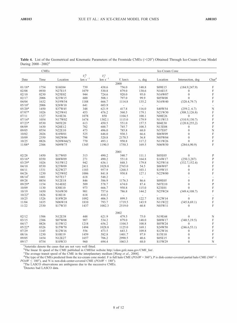
Table 4. List of the Geometrical and Kinematic Parameters of the Frontside CMEs (>120�) Obtained Through Ice-Cream Cone Model

During 2000–2002a

CMEs Ice-Cream Cone

Date Time LocationVf

b

km s�1Vf

c

km s�1 V, km/s a, deg Location Intersection, deg Chard

200001/18* 1754 S16E04 739 438.6 756.0 148.8 S09E15 (184.9,247.9) F02/08 0930 N27E15 1079 530.8 879.0 130.6 N16E15 0 F02/10 0230 N25E02 944 724.6 920.0 95.0 N16W07 0 F02/17 2006 S23W15 600 508.1 797.0 99.9 S05W08 0 F04/04 1632 N19W54 1188 666.7 1114.8 135.2 N16W40 (328.4,79.7) F05/10e 2006 S26W10 641 603.9 - - - - -05/20* 1450 S37W45 348 621.9 417.8 116.0 S40W54 (259.2, 6.7) N07/07* 1026 N23W41 453 476.2 560.5 179.1 N21W30 (308.3,126.8) F07/11 1327 N18E36 1078 850 1104.5 100.1 N08E26 0 F07/14* 1054 N17W02 1674 1302.1 1115.0 179.9 N11W13 (310.9,130.7) F07/23* 0530 N05E20 613 450.5 551.0 157.5 S04E30 (120.8,255,2) P08/09 1630 N20E12 702 688.7 745.7 108.3 N13E08 0 F09/05 0554 N22E10 473 496.0 785.8 68.0 N37E07 0 N10/02 2026 S10W01 525 646.0 930.3 66.6 S06W09 0 F10/09 2350 N02W06 798 520.8 2170.5 36.8 N05W04 0 F10/25 0826 N20W66(?) 770 493.1 950.8 117.2 N11W26 0 F11/08* 2306 N09W75 1345 1190.5 1750.3 169.5 N06W50 (284.6,90.9) F

200102/28 1450 S17W05 313 490.2 540.7 111.1 S05E05 0 P03/16* 0350 S08W09 271 490.2 551.0 164.8 S14W17 (250.3,287) P03/29* 1026 N15W12 942 636.1 848.3 179.8 N25W14 (332.7,152.4) F04/10 0530 S23W09 2411 1028.8 2765.0 54.5 S06W07 0 F04/11 1331 S22W27 1103 957.9 1268.5 103.1 S19W15 0 F04/26 1230 N23W02 1006 841.8 950.8 127.1 N22W00 0 F08/14f 1601 N37E17 618 548.2 - - - - -09/28 0854 N12E18 846 586.9 1176.3 86.6 S09E05 0 F09/29* 1154 N14E02 509 578.7 674.0 87.4 N07E10 0 P10/09 1130 S30E10 973 666.7 950.8 115.0 S23E01 0 F10/19 1650 N16W30 901 757.6 786.8 144.2 N25W24 (349.4,108.7) F10/22e 1826 S18E18 618 410.2 - - - - -10/25 1526 S18W20 1092 406.5 899.5 122.7 S12W14 0 F11/04 1635 N06W18 1810 793.7 1719.5 143.9 N11W22 (345.8,69.1) F11/22 2330 S17W35 1437 1082.3 2519.0 60.8 N03W11 0 F

200202/12 1506 N12E38 448 621.9 479.5 75.0 N19E44 0 N03/15 2306 S07W08 907 534.2 879.0 148.0 S00W17 (340.5,19.5) F04/17 0826 S13W12 1218 656.2 1104.5 108.8 S05W24 0 F05/22* 0326 S15W70 1494 1028.8 1125.0 169.1 S24W50 (246.6,53.1) F07/29 1145 S12W16 556 473.5 643.3 109.8 S12W16 0 F08/16 1230 S10E19 1459 582.8 1401.7 97.9 S15E10 0 F09/05 1654 N12E27 1657 706.2 2990.5 40.6 S05E15 0 F09/17 0754 S10W33 960 694.4 1063.5 68.0 S15W29 0 N

aAsterisks denote the cases that are not very well fitted.bThe linear fit speed of the CME published in CMElist website http://cdaw.gsfc.nasa.gov/CME_list/.cThe average transit speed of the CME in the interplanetary medium [Wang et al., 2004].dThe type of the CMEs predicted from the ice-cream cone model. F is full halo CME (POAW = 360�), P is disk-center-covered partial halo CME (360� <

POAW 180�), and N is non-disk-center-covered CME (POAW < 180�).eThe LASCO observations are ambiguous due to the successive CMEs.fDenotes bad LASCO data.


8 of 12

A08103

Figure 7. Comparison of the modeled halos (white circles) and the LASCO difference images for the28 October 2003 CME. The intersection region of the model with the sky plane is denoted by thecrosses.


9 of 12

A08103

partial halo CME here have no distinction in theprocess of the ice-cream model. They are different onlyon the LASCO observations because the partial CMEjust does not develop to a full halo in the view field ofLASCO observation, due to the orientation, angle width,and the radial distance of the ice-cream cone [Zhao etal., 2002].[32] The cases of ambiguous LASCO observations due

to successive CMEs erupted or bad LASCO observationaldata cannot be measured and are marked with e and f,respectively, in Table 4. The cases whose fitting projectedspeeds curves do not match the measured observationalprojected speeds data well are marked with stars in Table 4.The possible causes of these unmatched cases are described asfollowing: Some cases, i.e., the CMEs on 14 July 2000and 29 March 2001, whose angular widths are near 180�,are due to the very symmetrical LASCO observations andwith relatively deflected locations from the center of theSun; some cases have no relatively regular projectedcontours, i.e., the CMEs on 7 July 2000 and 16 March2001 or have no very clear observational pictures, i.e.,8 November 2000. The histograms of the speed distribu-tion and the angular width distribution are shown inFigures 8 and 9. The average speed of the CME is1104 km/s. The average width of the CME is approxi-mately equal to 114� (with the most narrow CME widthof 36.8� and the widest one of 179�).[33] In summary, we use an ice-cream cone model to

determine the geometrical and kinematical properties ofhalo CMEs as well as nonhalo CMEs. Comparing withthe previous cone model in the literature, there are somenew characteristics in this model.[34] First, the height-time relationship and the coordinate

system transformation are used in this model. From themeasurements of height-time relations in different azimuthalangles, one can get the nearly actual distributions of sky-plane observational speeds. It can avoid the ambiguities infinding the point which appears as the first above theocculting disk (that was used in the work of Michalek andGopalswamy [2003]). Moreover, it also give us a way to test

whether the parameters of a CME get from the model matchthe observation well.[35] Second, this method uses the SOHO/EIT observa-

tions to restrict the source locations to a relative smallregion. It will reduce calculating time and give relativelyaccurate locations near the active regions. For example,in the case of 4 April 2000, the fitted location is (q0,f0) = (74�, 40�) (that is, N16W40). This location is nearto the center the flare active region N19W56, while Xieet al.’s result (q0, f0) = (64.3�, 27.7�) (that is, N26W28)departs more from the flare region. From the Figure 4,one can also find this departure from the observationdata.[36] Third, we also use the ice-cream cone model to fit a

nonhalo CME. Halo CMEs and nonhalo CMEs have noessential differences in their geometrical and kinematicalproperties. The basic methods are the same only with someidentifications of observational measurements, namely,identification of the borders of yL, yR in equations inTable 1 from the LASCO observations. Similar work hasalso been done by Liu et al. [2002] using the methoddeveloped by Zhao et al. [2002].[37] Finally, the ice-cream cone model is different from

previous cone models in the intersectional region betweenthe cone and the sky plane. In this region, the projectionis determined by the top coronal of the ice-cream cone.For the event of 4 April 2000, the least-squares devia-tions calculated by the ice-cream cone model and thecone model are 77.2 km/s and 83.3 km/s, respectively.The difference is not very clear, which is due to the smallintersected angle IA = a/2 � g � 20� and cos IA � 0.94.For the event of 26 October 2003, the least-squaresdeviations obtained from the ice-cream cone model andthe cone model are 66.5 km/s and 132.8 km/s, respec-tively. Figure 10 shows the projected speed profiles for agiven CME with fixed parameters of V = 1000 km/s, a =120�, q = 90�, and the longitude f changing from 50� to80�. One can find that out of the intersectional region theice-cream cone model and the cone model give the same

Figure 8. The histogram showing the distribution of V forthe halo CMEs listed in Table 4.

Figure 9. The histogram showing the distribution of a forthe halo CMEs listed in Table 4.


10 of 12

A08103

results, but in intersectional region, they give very dif-ferent results.[38] Most of the slow CMEs (V < 250 km/s) show

acceleration while most of the fast CMEs (V > 900 km/s)show deceleration [Gopalswamy et al., 2000; Yashiro etal., 2004]. We have examined the height-time curve indifferent azimuths for each case listed in Table 4. In mostcases, we found that the height-time plots show nearlylinear relations in their measured azimuths with smallaccelerations (or decelerations). However, the accumulatedeffect of the small acceleration (or deceleration) willchange the initial and final speed of the CME due tothe large view field of LASCO. Thus the assumption ofconstant speed will be not suitable for some cases. This isone of the major error sources of this work. The othererror source may be that for simplicity, the apex of theice-cream cone is located in the center of the Sun, not atthe solar surface as done by Michalek and Gopalswamy[2003]. In general, the method in this paper works wellfor the fast CMEs whose front edges are clear in therunning different images. If the CME has relativelycomplex projected shape or the running different imagesare too faint, the result will be unstable.

[39] Acknowledgments. This work was supported by the ChineseAcademy of Sciences under grant KZCX-SW-136, the National NaturalScience Fund of China under grant 40336052 and 40474054, and theInnovation Fund of University of Science and Technology of China for thegraduate students KD2004031. We wish to acknowledge the use of datafrom the SOHO/LASCO and SOHO/EIT observer and the data from‘‘LASCO CME catalog.’’ We also acknowledge the two referees for criticalcomments and suggestions to improve this work.[40] Lou-Chuang Lee thanks G. Michalek and Xue-Pu Zhao for their

assistance in evaluating this paper.

ReferencesBrueckner, G. E., et al. (1995), The Large Angle Spectroscopic Corona-graph (LASCO), Sol. Phys., 162, 357.

Brueckner, G. E., J. P. Delaboudiniere, R. A. Howard, S. E. Paswaters,O. C. St. Cyr, R. Schwenn, P. L. Lamy, G. M. Simnett, B. Thompson,and D. Wang (1998), Geomagnetic storms caused by coronal massejections (CMEs): March 1996 through June 1997, Geophys. Res. Lett.,25, 3019.

Cane, H. V., and I. G. Richardson (2000), Interplanetary coronal massejections in the near-Earth solar wind during 1996–2002, J. Geophys.Res., 108(A1), 1156, doi:10.1029/2002JA009817.

Cane, H. V., I. G. Richardson, and O. C. St. Cyr (2000), Coronal massejections, interplanetary ejecta and geomagnetic storms, Geophys. Res.Lett., 27, 3591.

Delaboudiniere, J.-P., et al. (1995), EIT: Extreme-Ultraviolet Imaging Tele-scope for the SOHO mission, Sol. Phys., 162, 291.

Fisher, R. R., and R. H. Munro (1984), Coronal transient geometry. I- Theflare-associated event of 1981 March 25, Astrophys. J., 280, 428.

Gopalswamy, N. (2002), Space weather study using combined corona-graphic and in situ observations, in Space Weather Study Using Multi-point Techniques, COSPAR Colloq. Ser., edited by L.-H. Lyu, p. 39,Elsevier, New York.

Gopalswamy, N., A. Lara, R. P. Lepping, M. L. Kaiser, D. Berdichevsky,and O. C. St. Cyr (2000), Interplanetary acceleration of coronal massejections, Geophys. Res. Lett., 27, 145.

Gosling, J. T., D. J. McComas, J. L. Phillips, and S. J. Bame (1991),Geomagnetic activity associated with earth passage of interplanetaryshock disturbances and coronal mass ejections, J. Geophys. Res., 96,9831.

Harrison, R. A. (1986), Solar coronal mass ejections and flares, Astron.Astrophys., 162, 283.

Howard, R. A., D. J. Michels, N. R. Sheeley Jr., and M. J. Koomen (1982),The observation of a coronal transient directed at Earth, Astrophys. J.,263, L101.

Leblanc, Y., G. A. Dulk, A. Vourlidas, and J.-L. Bougeret (2001), Tracingshock waves from the corona to 1 AU: Type II radio emission andrelationship with CMEs, J. Geophys. Res., 106, 25,301.

Liu, W., S. P. Plunkett, and X. P. Zhao (2002), A cone model for coronalmass ejections, in Solar-Terrestrial Magnetic Activity and Space Envir-onment, COSPAR Colloq. Ser., edited by H. Wang and R. Xu, p. 267,Elsevier, New York.

Michalek, G., and N. Gopalswamy (2003), A new method for estimatingwidths, velocities, and source location of halo coronal mass ejections,Astrophys. J., 584(1), 472.

Michalek, G., N. Gopalswamy, A. Lara, and P. K. Manoharan (2004),Arrival time of halo coronal mass ejections in the vicinity of the Earth,Astron. Astrophys., 423, 729.

Plunkett, S. P., B. J. Thompson, O. C. St. Cyr, and R. A. Howard (2001),Solar source regions of coronal mass ejections and their geomagneticeffects, J. Atmos. Sol. Terr. Phys., 63, 389.

Figure 10. The projection speed profiles on the sky plane for a given CME with V = 1000 km/s, a =120�, q = 90�, and f changing from 50� to 80�. The results obtained from the ice-cream cone model andthe cone model are shown by the solid line and the dashed line, respectively. The intersection regionbetween the cone and the sky plane is indicated by the horizontal line.


11 of 12

A08103

Tsuneta, S., L. Acton, M. Bruner, J. Lemen, W. Brown, R. Caravalho,R. Catura, S. Freeland, B. Jurcevich, and J. Owens (1991), The soft X-raytelescope for the SOLAR-A mission, Sol. Phys., 136, 37.

Wang, Y. M., P. Z. Yee, S. Wang, G. P. Zhou, and J. X. Wang (2002), Astatistical study on the geoeffectiveness of Earth-directed coronal massejections from March 1997 to December 2000, J. Geophys. Res.,107(A11), 1340, doi:10.1029/2002JA009244.

Wang, Y., C. L. Shen, S. Wang, and P. Z. Ye (2004), Deflection ofcoronal mass ejection in the interplanetary medium, Sol. Phys., 222,329.

Webb, D. F., S. W. Kahler, P. S. McIntosh, and J. A. Klimchuck (1997),Large-scale structures and multiple neutral lines associated with coronalmass ejetcions, J. Geophys. Res., 102, 24,161.

Webb, D. F., E. W. Cliver, N. U. Crooker, O. C. St. Cyr, and B. J. Thompson(2000), Relationship of halo coronal mass ejections, magnetic clouds, andmagnetic storms, J. Geophys. Res., 105, 7491.

Xie, H., L. Ofman, and G. Lawrence (2004), Cone model for halo CMEs:Application to space weather forecasting, J. Geophys. Res., 109, A03109,doi:10.1029/2003JA010226.

Yashiro, S., N. Gopalswamy, G.Michalek, O. C. St. Cyr, S. P. Plunkett, N. B.Rich, and R. A. Howard (2004), A catalog of white light coronal massejections observed by the SOHO spacecraft, J. Geophys. Res., 109,A07105, doi:10.1029/2003JA010282.

Zhao, X. P., S. P. Plunkett, and W. Liu (2002), Determination of geometricaland kinematical properties of halo coronal mass ejections using the conemodel, J. Geophys. Res., 107(A8), 1223, doi:10.1029/2001JA009143.

��X. K. Dou, C. B. Wang, and X. H. Xue, School of Earth and Space

Sciences, University of Science and Technology of China, Hefei, Anhui,230026, China. ([email protected]; [email protected]; [email protected])


12 of 12

A08103

an ice-cream cone model for coronal mass...

Documents