An Illustration of the Average Exit Time Measure of Poverty

John Gibson and Susan Olivia*

University of Waikato

Abstract

The goal of the World Bank is ‘a world free of poverty’ but the most widely used poverty

measures do not show when poverty might be eliminated. The ‘head-count index’ simply

counts the poor, while the ‘poverty gap index’ shows their average shortfall from the

poverty line. Neither measure reflects changes in the distribution of incomes amongst the

poor, but squaring the poverty gap brings sensitivity to inequality, albeit at the cost of

intuitive interpretation. This paper illustrates a new measure of poverty [Morduch, J.,

1998, Poverty, economic growth and average exit time, Economics Letters, 59: 385-390].

This new poverty measure is distributionally-sensitive and has a ready interpretation as

the average time taken to exit poverty with a constant and uniform growth rate.

JEL: I32, O15

Keywords: Growth, Inequality, Poverty

*Department of Economics, University of Waikato, Private Bag 3105, Hamilton, New Zealand. Phone: (64-7) 856-2889. Fax: (64-7) 838-4331. Email: jkgibson@waikato.ac.nz

1

I. Introduction

The goal of the World Bank is ‘a world free of poverty’. To measure progress in meeting this

goal, the World Bank regularly prepares and publishes estimates of the number of poor people in

the world. It is well known that simply counting the poor and calculating their proportion in the

population can be a misleading indicator of poverty because no allowance is made for how far

below the poverty line they fall (other problems with these world poverty counts are discussed by

Deaton, 2000). A further problem with this head-count measure of poverty is that it may give

perverse incentives to target poverty reduction towards the least poor because a given transfer will

push more of them over the poverty line. Even ‘poverty gap’ measures, based on the average

shortfall between the incomes of the poor and the poverty line, can be criticised because they are

invariant to regressive transfers to a poor person from someone who is poorer (Sen, 1976).

But despite these shortcomings, the head-count and poverty gap measures remain the most

widely used indicators of poverty, and this popularity may not just reflect their simplicity. Other

poverty indicators that are sensitive to inequality amongst the poor, and thus are superior on

theoretical grounds, may convey less meaningful information because these measures can be

interpreted only in an ordinal sense (Foster, 1994). Thus, even though the poverty gap can be

transformed into an inequality-sensitive measure, by squaring or cubing it (Foster, Greer,

Thorbecke, 1984), such a transformation may reduce the cardinal usefulness of the measure.

Differences between poverty measures that satisfy theoretical axioms but have only ordinal

interpretations and simpler measures with direct, cardinal, meaning would not matter if all poverty

measures always gave the same conclusions. But determining the effect of particular economic

policies often depends on the choice of poverty measure. For example, if the price of rice rises in

2

Java, Indonesia, headcount measures of poverty fall because most poor households are farmers,

who are net producers of rice. But distributionally-sensitive poverty measures rise because the

very poorest households are net rice consumers, and this group get the biggest weight in measures

that are sensitive to inequality (World Bank, 1990, p.28).

This paper illustrates a new measure of poverty that has been developed by Morduch (1998)

from an existing measure (the Watts index) that has appealing ordinal properties. Morduch shows

that a simple linear transformation of the Watts index gives it cardinal properties that can be useful

as well. Hence, wider use of the poverty measure developed by Morduch might overcome the

dilemma between distributionally-sensitive measures on the one hand and cardinally meaningful

measures on the other. This poverty measure is sensitive to inequality amongst the poor (indeed, it

nests the common Theil measure of inequality) and it has a ready interpretation as the average time

taken to exit poverty with a constant and uniform growth rate. Thus, the measure illustrates an

aspect of the income distribution that is associated with an interesting economic question – how

long might it take to be free of poverty? Yet despite its potential usefulness, the average exit time

measure is yet to have an impact on the empirical poverty literature.1

While it would be possible to illustrate the use of this new poverty measure with world-wide

estimates of poverty, that task is beyond the current paper. Instead, we use data from the

developing country of Papua New Guinea to calculate poverty values using the average exit time

measure and some other well-known measures. This particular country has the highest degree of

inequality in the Asia-Pacific region, with a Gini coefficient of 0.51 for per capita expenditures

(World Bank, 2001).2 Hence, this is a setting where distributionally-sensitive poverty measures

may be especially applicable, but it is also a setting that needs easily interpretable measures

3

because few policy makers have advanced education.

II. Poverty Axioms And Poverty Measures

A. Poverty Axioms

There are a variety of axioms that a desirable poverty measure should obey, with the two most

fundamental proposed by Sen (1976):

Monotonicity Axiom: Other things being equal, a reduction in income of a person below

the poverty line should increase the poverty measure.

Transfer Axiom: Other things being equal, a transfer of income from a person below

the poverty line to a person who is richer must increase the

poverty measure.

In addition, Kakwani (1980) proposed the monotonicity-sensitivity and transfer-sensitivity axioms.

Under the monotonicity-sensitivity axiom, the poorer an individual is, the larger should be the

increase in the poverty index due to a reduction in their income. The transfer-sensitivity axioms

suggest that society should become less concerned about inequality between poor people as they

become richer. For example, if A and B have incomes of $100 and $50, then transferring $1 from

A to B should reduce the poverty index by at least as much as would a similar transfer when A and

B have incomes of $300 and $250.

In addition to these axioms, the property of additive decomposability is considered desirable

because it means that the poverty index for a given society is just a weighted average of the

poverty indexes for sub-groups in the society. Thus, if the population shares for these sub-groups

stay constant, an increase in the level of poverty in one sub-group will increase overall poverty.

4

This property helps in the construction of poverty profiles, which show how poverty varies across

population sub-groups and how each sub-group contributes to overall poverty.

B. Some Existing Poverty Measures

A widely used class of poverty measures is due to Foster, Greer and Thorbecke (1984) -

hereafter FGT. Say y=(y1, y2…yn) is a vector of incomes ranked from lowest to highest. A poverty

line z is an income level such that, by definition, people whose incomes are lower than z are poor,

and an individual' s poverty gap is defined as:

.0 zy

zyyzg

j

jjj

>=

≤−=

The general formula for the FGT class of poverty measures is:

01

1≥∑

=

=α

α

α

q

j

j

z

g

nP (1)

where n is the total population, and q is the number of poor persons. The parameter α reflects

poverty aversion; larger values put higher weight on the poverty gaps of the poorest people. If

α=0, equation (1) reduces to q/n, which is the commonly used head-count ratio, H. Setting α=1

amounts to aggregating the proportionate poverty gaps, which shows the shortfall of the poor’s

income from the poverty line expressed as an average over the whole population. This gives the

normalised poverty gap measure, PG. For example, with a poverty line of $1000 and a population

of four persons, two of whom have incomes of $700 and two of whom have incomes above the

poverty line, %154)3.03.0( =+=PG (or alternatively, an aggregate poverty gap of $600

expressed as a ratio to ).4000$=× zn Setting α=2 amounts to weighting each proportionate gap

5

by itself and this squared poverty gap is a distributionally-sensitive measure, which is often called

the poverty severity index, PS. Continuing the previous example, if $200 is taken from one of the

poor persons and given to the other, the PG measure will not change because the average shortfall

from the poverty line is unchanged, but the poverty severity index will increase from

%5.44)3.03.0( 22 =+ to %.5.64)5.01.0( 22 =+ These three poverty indicators, H, PG, and PS

are widely used in World Bank poverty assessments and in the academic literature on poverty,

although Sen’s monotonicity axiom is satisfied only for α>0, the transfer axiom is satisfied only for

α>1, and Kakwani’s transfer-sensitivity axiom is satisfied only for α>2.

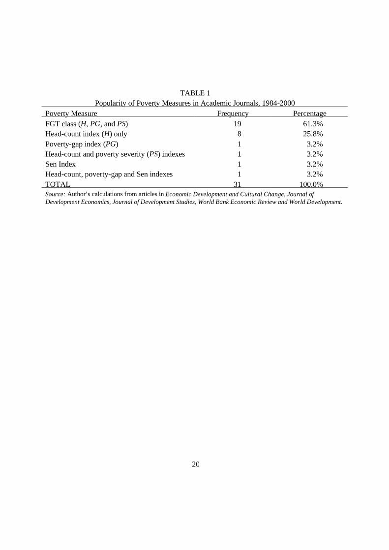
The popularity of the FGT class of poverty measures is shown in Table 1, which reports

frequency of use for various poverty measures. The sample is empirical (quantitative) articles

about poverty in five leading journals in development economics over the 1984-2000 period. In

addition to measures from the FGT class, the other poverty measure shown in Table 1 is the Sen

Index, which combines head-count and poverty gap measures with the Gini coefficient measuring

inequality amongst the poor.

Almost two-thirds of the articles use the FGT class of poverty measures, with α=0,1, and 2.

However, it is also notable that one-quarter of the academic articles just use the head-count index,

in spite of the fact that this measure satisfies none of the standard axioms. This continued use of

the head-count index suggests that for many purposes a poverty measure that is cardinally

meaningful is more useful than measures that obey the various axioms. It is also the experience of

the authors, that even when using the FGT class of poverty measures, it is easiest to discuss and

interpret the head-count and poverty-gap indexes, in contrast to the poverty-severity index (α=2)

6

which has only an ordinal interpretation.

III. The Average Exit Time Measure Of Poverty

To derive the average exit time measure of poverty, Morduch (1998) starts with an existing

distributionally-sensitive measure, due to Watts (1968):

[ ]∑ −==

q

jjyz

nW

1)(ln)(ln

1 (2)

where there are j individuals in the population indexed from 1 to n in ascending order of (positive)

income and q is the number of people with income yj below the poverty line z. Despite being

sensitive to inequality amongst the poor, additively decomposable, and satisfying the transfer-

sensitivity axiom (unlike the PS index), the Watts measure has not proven popular, as Table 1

indicates. This lack of use may be because, in common with other distributionally-sensitive

measures (including the PS index), the Watts measure of poverty has no cardinal interpretation.

However, Morduch (1998) shows that simply dividing the Watts poverty measure by some

hypothetical growth rate g, where g>0, gives it an interesting cardinal interpretation. This

transformed index reflects the average number of years that it would take the population to exit

poverty if it were possible to ensure that all incomes grow at rate g. In other words, this average

exit time maps the income distribution to the space of time. It thus provides a simple metric of the

potential for economic growth to reduce poverty and in this way it may help to illuminate a

contested policy debate (see, for example, Dollar and Kraay, 2000).

Morduch (1998) shows that if the income of a poor person, yj grows at a constant positive rate

g per year, the number of years it will take them to reach the poverty line is:

7

.)(ln)(ln

g

yzt

jjg

−= (3)

For example, if the poverty line is set at $1000, someone with an income of $700 that grows by

3% per year will reach the poverty line, and hence exit poverty, after 12 years. The average exit

time is simply jgt averaged over the whole population, including the non-poor for whom

jgt =0:

)4(.)(ln)(ln11

11gW

g

yz

Nt

NT

jq

j

N

j

jgg =

−∑=∑===

In addition to the average exit time across the whole population, Tg, the average exit time just for

the poor can be obtained, either from a separate calculation on the sub-sample of poor households,

or more directly by scaling up by the head-count ratio of poverty: .HTg

Because equation (4) is just a transform of the Watts index, the sensitivity to inequality is

preserved. Carrying on the example of a poverty line of $1000 and a growth rate of 3%, for

someone whose income is $900 it takes 3.5 years to exit poverty while for someone whose income

is only $500 it would take 23.1 years to reach the poverty line. Thus the average exit time in this

two-person society is 13.3 years [(3.5+23.1)/2], which is higher than the 12 year exit time that

would apply if the incomes of these two persons were equalised at $700. The sensitivity to

inequality occurs because the average exit time measure nests the Theil index of inequality, in

much the same way that the Sen index nests the Gini coefficient (Morduch, 1998).

8

IV. A Poverty Profile For Papua New Guinea

To compare the performance of the average exit time measure of poverty with that of the more

familiar FGT class of poverty measures, data are used from a 1996 survey of households in Papua

New Guinea, collected for a World Bank poverty assessment (Gibson, 2000). This survey

measured the expenditures of a random sample of 1144 households, located in 73 rural and 47

urban communities. The survey did not attempt to measure incomes, but this is no disadvantage

because expenditure is the preferred monetary indicator of living standards when measuring

poverty (Deaton, 2000). In addition to the ‘clustering’ of the data, the sample was weighted and

stratified, so the results reported below take account of these sample design features.

There is considerable spatial price variation in Papua New Guinea because of the rugged

terrain and poor transport infrastructure. To control for this variation, a spatial price index (set for

five different regions) was applied to the nominal expenditure estimates for each household, so as

to convert them into national average prices prior to the calculation of the poverty measures. This

spatial price index was based on a “cost-of-basic-needs” poverty line (Ravallion and Bidani, 1994)

calculated from the cost of a diet of locally consumed foods providing 2200 calories per day, with

an additional allowance for non-food spending. The household expenditures are also deflated for

differences in household size and composition by dividing by the number of adult-equivalents,

where children aged 0-6 years count as 0.5 of an adult (Gibson, 2000). The average value of

deflated household expenditures is K900 per adult-equivalent per year (US$700 at the market

exchange rate of US$0.76 prevailing at the time of the survey). However, there is a considerable

skew in the distribution of expenditures, so the median expenditure level is only K580 (or K510 in

per capita terms when no allowance is made for differences in consumption needs of children and

9

adults).

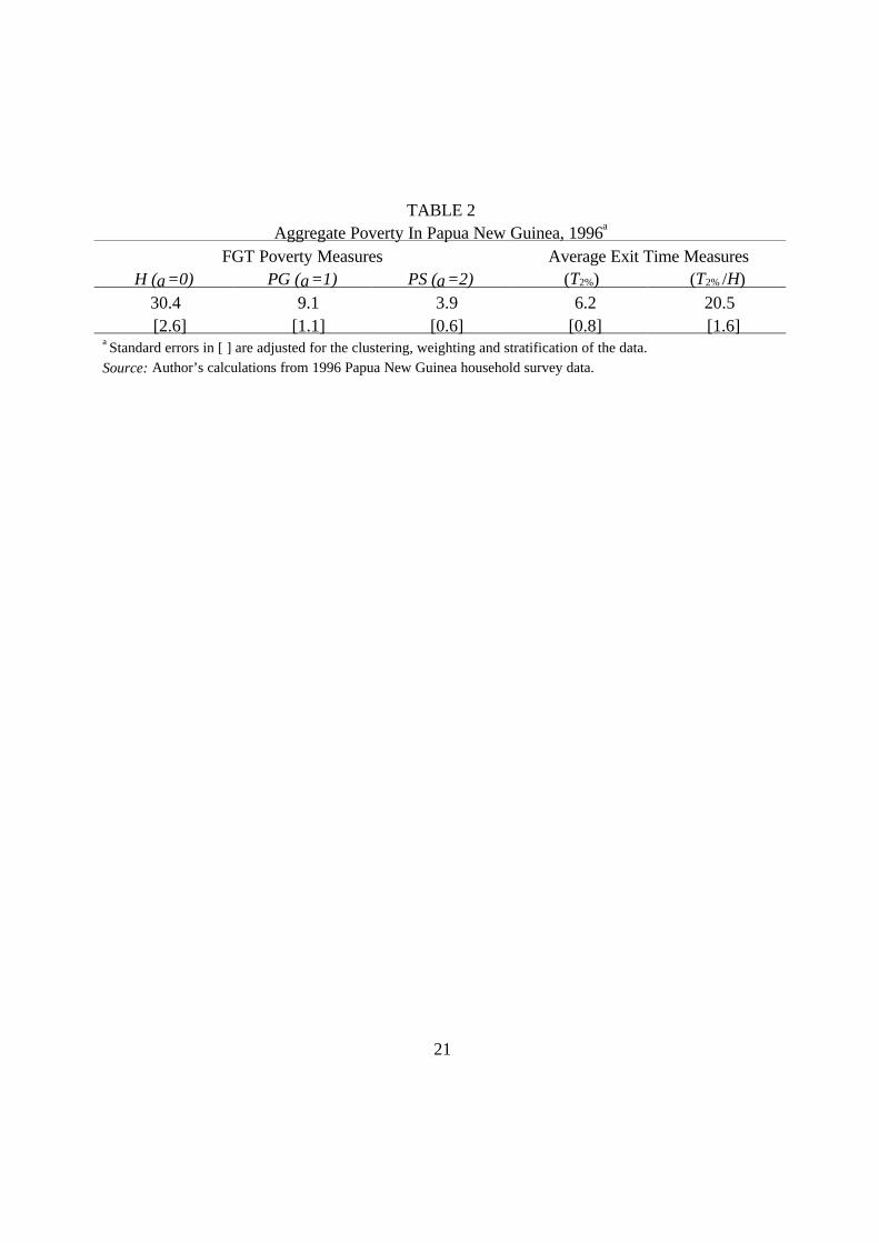
Table 2 reports the FGT and average exit time poverty measures for Papua New Guinea in

1996. These poverty measures are based on a cost-of-basic-needs poverty line of K400 per adult-

equivalent per year. The first two FGT poverty measures show that 30.4% of the population are

classified as poor and that the aggregate poverty gap is equivalent to 9.1% of the value of the

poverty line averaged over the whole population (equivalently, a gap of 30% averaged over just

the poor). The aggregate shortfall from the poverty line can also be calculated in monetary terms,

by multiplying the PG index by the value of the poverty line and by the population size (4.3 million

adult-equivalents). This calculation shows that it would require perfectly targeted (and costless)

transfers of K160m per year to eliminate poverty in Papua New Guinea. Although the magnitude

of these first two poverty indicators, H and PG, is easily grasped, neither of them reflects the

distribution of living standards amongst the poor. The poverty severity index, which is sensitive to

inequality amongst the poor, has a value of 3.9% but there is no easily intuitive interpretation of

this value, except in comparison to other values of the same index.

The average exit time measures in Table 2 are calculated for a potential growth rate of real

consumption per adult-equivalent of 2% per year, which is consistent with the medium-term

performance of the Papua New Guinea economy. The average time taken to exit poverty would be

6.2 years if this growth rate was continuous and uniform across the population. This is clearly an

unrealistic, best-case, scenario because growth is rarely uniform and even more rarely continuous.

However, the poverty gap measure conveys meaningful information under equally unrealistic

conditions – perfect targeting and costless redistribution – but that has not diminished its

usefulness.

10

One reason why the average exit time is ‘only’ 6.2 years is that more than two-thirds of the

population are above the poverty line, so their exit time is zero. The more useful indicator for

policy discussions may be the average exit time amongst the poor because otherwise policy makers

might conclude that poverty can be quickly eliminated, neglecting to remember that many people

are already non-poor. The average exit time for the poor population in Papua New Guinea is 20.5

years with a 2% annual growth rate. It is also possible to demonstrate the contribution of

inequality to this average exit time. The average expenditure level of the poor is K280 per adult-

equivalent per year,3 and starting from this point and growing by 2% per year, it would take 17.8

years to reach the poverty line. The exit time using the average income of the poor can be denoted

avggt and Morduch (1998) shows that this is related to the average exit time of the poor by:

gavggg LtHT += (5)

where Lg is the Theil index of inequality amongst the poor, divided by the growth rate g. Thus, in

Papua New Guinea inequality amongst the poor adds almost three years to their average exit time.

How does the pattern of poverty vary across population sub-groups in Papua New Guinea?

Table 3 reports sub-group poverty estimates and contributions to total poverty for three splits of

the population; urban versus rural, male-headed versus female-headed households, and households

headed by illiterates versus those headed by someone who can read. These splits are chosen to

illustrate particular aspects of the poverty measures, although they are also common in poverty

profiles because of their policy implications.

All poverty measures are considerably lower in the urban sector of Papua New Guinea but the

gap between the sectors becomes especially apparent when using distributionally-sensitive

11

measures. While the head-count index for the rural population is approximately three times that of

the urban population, the expected number of years to exit poverty is five times that of the rural

sector and the poverty severity index is five times higher. The increasing ‘ruralness’ of poverty as

the poverty index becomes distributionally-sensitive can also be shown using the additive

decomposability property of both the FGT and average exit time poverty measures. The results in

the bottom half of Table 3 show that while the urban sector contains 15% of the population, it has

only 5.8% of the head-count poor and contributes even less to either the average exit time or to

the poverty severity index (3.4% and 2.7%).

The comparison of poverty rates for male-headed and female-headed households illustrates the

importance of relying on more than just the head-count index of poverty. At first glance, it appears

that poverty is higher for those in female-headed households, with the head-count rate five

percentage points higher. However, all of the other poverty measures suggest the opposite

conclusion. The average income of poor, male-headed, households is lower than that of poor,

female-headed, households (also shown by the larger PG index) and it would take a poor person in

a male-headed household an average of six years more to exit poverty. Calculating avggt from the

average expenditure levels of K277 and K305 for male-headed and female-headed households

shows that five years of this gap is due to the lower income of the male-headed households, and

one year of the gap is due to the greater inequality (a Theil index of 0.052 for poor, male-headed

households versus 0.027 for female-headed households).

The reinforcing effects of a lower average and a greater inequality in expenditures amongst the

poor is also apparent in the effects of literacy on poverty. Inequality amongst the poor whose

12

household head is illiterate raises their average exit time by 3 years, as opposed to only a 1.5 year

increase amongst the ‘literate poor’. Thus, the group with illiterate household heads make an even

larger contribution – two-thirds or more – to the T2% and PS indexes than to the head-count

index. In general, across the three population splits in Table 3, the average exit time measure

shows similar patterns to the more widely used PS index.

Because the average exit time maps a static income distribution into the dimension of time,

raising the growth rate in the calculation automatically reduces exit times, and so may be

uninformative (Morduch, 1998). But there could be heuristic value in such an exercise if it can

demonstrate a potential effect of unbalanced growth. For example, if annual consumption growth

in the rural sector is only, say, 1% while in the urban sector it is 3%, this unbalanced growth

combines with the initially lower incomes in the rural sector to produce a large gap in exit times.

This is apparent from Figure 1, which shows HTg for each sector as g varies. At a 1% growth

rate, the average exit time for the poor in rural areas is 42 years, while at a 3% growth rate the

average exit time for the urban poor is only 7.5 years. This gap of 35 years may catch the attention

of policy makers more than simply reporting the 2% difference in sector growth rates.

V. Temporal Poverty Comparisons

In addition to describing the cross-sectional pattern of poverty, the average exit time measure

can also be used for temporal comparisons, to test whether poverty is increasing. In Papua New

Guinea, the only previous poverty estimates are for the capital city, Port Moresby, and are based

on a survey of 325 households in 1986. The expenditure estimates from this survey do not include

13

services from dwellings and durables (in contrast to the estimates used above) and the poverty line

has a more generous allowance for non-food items. Therefore the expenditure estimates for the

106 households in the 1996 survey from Port Moresby were adjusted to be comparable with the

earlier data, and the poverty line was updated from its 1986 value of K620 (in the higher capital

city prices rather than in national average prices).

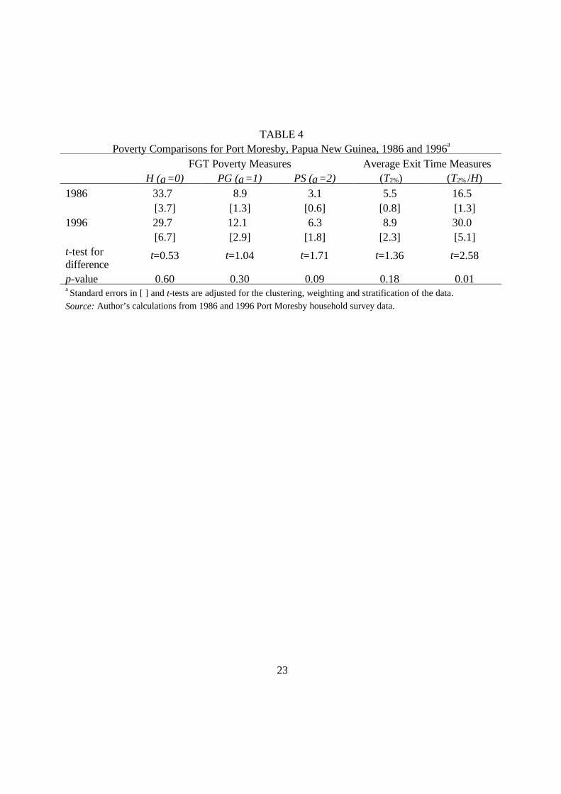
With these adjusted expenditures and poverty lines, the head-count poverty rate in 1986 is

33.7% and in 1996 it is 29.7%. This difference is not statistically significant (p<0.60) so policy

makers might be tempted to conclude that there had been no change in poverty over this 10-year

period, at least in Port Moresby. A similar conclusion would be reached when using the poverty

gap index, which although rising, does so in a statistically insignificant way.

However, a much different message about the change in poverty comes from the

distributionally-sensitive measures. The poverty severity index doubled between 1986 and 1996

and the hypothesis of no change in poverty rates would be rejected, at least at the p<0.10 level.

This rise in the PS index while the head-count poverty rate is falling suggests a substantial

worsening of the income distribution amongst the poor. Reflecting this rising inequality, one

would also expect the average exit time for the poor to rise. Table 4 shows this effect clearly, with

HT %2 increasing by 13.5 years during this period, which is a statistically significant change

(p<0.02). Further evidence on the rise in inequality comes from the Theil index for the poor, which

increased from 0.026 to 0.076. When rescaled into units of time, inequality amongst the poor

added 1.3 years to their average exit time in 1986 and 3.8 years in 1996. The remaining 11-year

increase in HT %2 is due to the fall in the average living standards of the poor, with mean

14

expenditures at only 59% of the poverty line in 1996, compared with 74% in 1986.

These divergent trends in poverty measures since 1986 once again emphasise the importance

of using poverty indicators that are sensitive to inequality amongst the poor – poverty is about

much more than just how many are poor and how big is their average shortfall from the poverty

line. Even though the average exit time measure is designed to demonstrate the potential effects of

growth on poverty, it is also a useful tool in settings, such as Port Moresby, where a major

contributor to poverty appears to be rising inequality amongst the poor.

VI. Conclusions

This paper has demonstrated the practical usefulness of the average exit time measure of

poverty developed by Morduch (1998). This average exit time measure of poverty is

distributionally-sensitive, additively decomposable and satisfies the standard poverty axioms and

its performance in cross-sectional and temporal poverty comparisons is shown here to be

comparable to that of the more widely used poverty severity index. But a key advantage of the

average exit time is that it is cardinally meaningful; the particular values of this poverty measure

can be used to answer an interesting economic question: under best-case conditions of continuous

and evenly distributed growth, how long would it take to be free of poverty?

Using the average exit time measure, as either a supplement to the popular FGT poverty

measures or else as a replacement for the poverty severity index, does not reduce the need for

poverty analysts to develop data-sets that show the actual dynamics of poverty. The limited set of

longitudinal studies available in developing countries show that many people move repeatedly into

and out of poverty (see, for example, World Bank, 1990, p.35). Rather than being a replacement

15

for the data needed to study this transient poverty, the average exit time measure provides a

framework for thinking about what a given income distribution implies about the dynamics of

poverty reduction. Indeed, the average exit time measure could be used as a type of frontier for

exercises that use actual longitudinal data on poverty spells to measure the cost – in terms of

longer duration of poverty – of unevenly distributed and unstable economic growth.

16

Notes

1 The Social Science Citation Index records only one article that has cited Morduch (1998), and

this reference is only as an aside. Hence, except for the initial illustrations by Morduch himself, the

average exit time measure does not appear to have been used in applied poverty research.

2 In comparison, the Philippines which is usually considered to have a high degree of inequality,

has a Gini coefficient of only 0.46.

3 This average can be calculated as ( ) zHPG × , or (0.091/0.304)×400 in the current case.

17

Acknowledgments

*The data used for this paper were originally collected as part of a project on poverty in Papua

New Guinea, funded by the World Bank with support from the governments of Australia

(TF-032753), Japan (TF-029460) and New Zealand (TF-033936). The comments of Jeffrey

Nugent, Nola Reinhardt, John Tressler and participants at the Western Economic Association

conference are gratefully acknowledged.

18

References

Deaton, A. (2000). Counting the World’s Poor: Problems and Possible Solutions. (Mimeo)

Princeton, NJ: Research Program in Development Studies, Princeton University.

Dollar, D., & Kraay, A. (2000). Growth is Good for the Poor. Washington, DC: The World Bank.

Foster, J., (1994). Normative measurement: Is theory relevant? American Economic Review,

84 (2), 365-370.

Foster, J., Greer, J. & Thorbecke, E. (1984). A class of decomposable poverty measures.

Econometrica, 52 (3), 761-766.

Gibson, J. (2000). The Papua New Guinea Household Survey. Australian Economic Review,

33 (4), 377-380.

Kakwani, N. (1980). On a class of poverty measures. Econometrica, 48 (2), 437-446.

Morduch, J. (1998). Poverty, Economic growth and average exit time. Economics Letters,.

59 (3), 385-390.

Ravallion, M., & Bidani, B. (1994). How robust is a poverty profile? The World Bank

Economic Review, 8 (1), 75-102.

19

Sen, A.K., (1976). Poverty: An ordinal approach to measurement. Econometrica, 44 (2), 219-231.

Watts, H., (1968). An economic definition of poverty. In Daniel P. Moynihan (Ed),

Understanding Poverty (pp. 316-329). New York: Basic Books.

World Bank, (1990). World Development Report. New York: Oxford University Press.

World Bank, (2001). World Development Indicators. New York: Oxford University Press.

20

TABLE 1 Popularity of Poverty Measures in Academic Journals, 1984-2000

Poverty Measure Frequency Percentage FGT class (H, PG, and PS) 19 61.3% Head-count index (H) only 8 25.8% Poverty-gap index (PG) 1 3.2% Head-count and poverty severity (PS) indexes 1 3.2% Sen Index 1 3.2% Head-count, poverty-gap and Sen indexes 1 3.2% TOTAL 31 100.0% Source: Author’s calculations from articles in Economic Development and Cultural Change, Journal of Development Economics, Journal of Development Studies, World Bank Economic Review and World Development.

21

TABLE 2 Aggregate Poverty In Papua New Guinea, 1996a

FGT Poverty Measures Average Exit Time Measures H (α=0) PG (α=1) PS (α=2) (T2%) (T2% /H)

30.4 [2.6]

9.1 [1.1]

3.9 [0.6]

6.2 [0.8]

20.5 [1.6]

a Standard errors in [ ] are adjusted for the clustering, weighting and stratification of the data. Source: Author’s calculations from 1996 Papua New Guinea household survey data.

22

TABLE 3 Distribution of Poverty by Population Sub-Groups in Papua New Guinea

Location Characteristics of Household Head Rural Urban Male Female Literate Illiterate Head-count index (H) 33.6 11.8 30.0 35.4 22.1 40.6 Poverty gap index (PG) 10.4 2.3 9.2 8.4 5.9 13.2 Poverty severity (PS) 4.5 0.7 4.0 3.0 2.2 6.1 Average exit time (T2%) 7.1 1.4 6.3 5.3 3.8 9.2 T2% /H 21.0 11.9 20.9 14.9 17.1 22.7 Mean income of poor 277 322 277 305 293 270 Contribution to total Population 85.0% 15.0% 93.5% 6.5% 55.4% 44.6% Head-count index (H) 94.2% 5.8% 92.4% 7.6% 40.4% 59.6% Poverty gap index (PG) 96.2% 3.8% 94.0% 6.0% 35.8% 64.2% Poverty severity (PS) 97.3% 2.7% 95.1% 4.9% 30.9% 69.1% Average exit time (T2%) 96.6% 3.4% 94.5% 5.5% 33.8% 66.2% Source: Author’s calculations from 1996 Papua New Guinea household survey data.

23

TABLE 4 Poverty Comparisons for Port Moresby, Papua New Guinea, 1986 and 1996a

FGT Poverty Measures Average Exit Time Measures H (α=0) PG (α=1) PS (α=2) (T2%) (T2% /H)

1986 33.7 [3.7]

8.9 [1.3]

3.1 [0.6]

5.5 [0.8]

16.5 [1.3]

1996 29.7 [6.7]

12.1 [2.9]

6.3 [1.8]

8.9 [2.3]

30.0 [5.1]

t-test for difference

t=0.53 t=1.04 t=1.71 t=1.36 t=2.58

p-value 0.60 0.30 0.09 0.18 0.01 a Standard errors in [ ] and t-tests are adjusted for the clustering, weighting and stratification of the data.

Source: Author’s calculations from 1986 and 1996 Port Moresby household survey data.

24

FIGURE 1Average Exit Time of the Poor Population

0

5

10

15

20

25

30

35

40

45

0 0.01 0.02 0.03 0.04 0.05 0.06 0.07

Growth rate

Yea

rs

RuralUrban