beyond the headcount: examining the dynamics and patterns of multidimensional poverty in indonesia
DESCRIPTION
The aim of this study was twofold. First, although a number of empirical studies exist on income poverty in Indonesia, very few have examined multidimensional household welfare deprivations. We attempted to fill this gap by using for the first time the annually conducted National Socioeconomic Survey by Statistics Indonesia (BPS), and the Alkire and Foster (2007; 2011) methodology to investigate the degree and dynamics of multidimensional household welfare deprivations in Indonesia for the 2004 and 2013 time periods. Second, we explore whether there are differing patterns of change for consumption poverty and multidimensional poverty at both the household and regional level. We investigate the magnitude of overlap between consumption and multidimensional poverty, and explore whether the multidimensionally deprived households are necessarily income poor or not and vice versa. In particular we scrutinize whether the question of who is poor has many different answers.TRANSCRIPT
TIM NASIONALPERCEPATAN PENANGGULANGAN KEMISKINAN
TNP2KWORKING PAPER
BEYOND THE HEADCOUNT: EXAMINING THE DYNAMICS AND PATTERNS OF MULTIDIMENSIONAL POVERTY IN INDONESIA
TNP2K WORKING PAPER 21-2014December 2014
SUDARNO SUMARTO AND INDUNIL DE SILVA


TNP2K WORKING PAPER 21-2014December 2014
SUDARNO SUMARTO AND INDUNIL DE SILVA
The TNP2K Working Paper Series disseminates the findings of work in progress to encourage discussion and exchange of ideas on poverty, social protection, and development issues.
Support for this publication has been provided by the Australian Government through the Poverty Reduction Support Facility (PRSF).
The findings, interpretations, and conclusions herein are those of the author(s) and do not necessarily reflect the views of the Government of Indonesia or the Government of Australia.
You are free to copy, distribute, and transmit this work for noncommercial purposes.
Suggested citation: Sumarto, Sudarno and Indunil De Silva. 2014. ‘Beyond the Headcount: Examining the Dynamics and Patterns of Multidimensional Poverty in Indonesia’. TNP2K Working Paper 21-2014. Jakarta, Indonesia: Tim Nasional Percepatan Penanggulangan Kemiskinan (TNP2K).
To request copies of the paper or for more information, please contact the TNP2K Knowledge Management Unit ([email protected]). This and other TNP2K publications are also available at the TNP2K website (www.tnp2k.go.id).
BEYOND THE HEADCOUNT: EXAMINING THE DYNAMICS AND PATTERNS OF MULTIDIMENSIONAL POVERTY IN INDONESIA
TNP2KGrand Kebon Sirih Lt.4,Jl.Kebon Sirih Raya No.35,Jakarta Pusat, 10110Tel: +62 (0) 21 3912812Fax: +62 (0) 21 3912513www.tnp2k.go.id

iv
v
Beyond the Headcount: Examining the Dynamics and Patterns of Multidimensional Poverty in Indonesia
Sudarno Sumarto and Indunil De Silva1
December 2014
ABSTRACT
The aim of this study was twofold. First, although a number of empirical studies exist on income poverty in Indonesia, very few have examined multidimensional household welfare deprivations. We attempted to fill this gap by using for the first time the annually conducted National Socioeconomic Survey by Statistics Indonesia (BPS), and the Alkire and Foster (2007; 2011) methodology to investigate the degree and dynamics of multidimensional household welfare deprivations in Indonesia for the 2004 and 2013 time periods. Second, we explore whether there are differing patterns of change for consumption poverty and multidimensional poverty at both the household and regional level. We investigate the magnitude of overlap between consumption and multidimensional poverty, and explore whether the multidimensionally deprived households are necessarily income poor or not and vice versa. In particular we scrutinize whether the question of who is poor has many different answers.
This paper is innovative in that it changes the focus from the conventional unidimensional perspective of poverty, centered on income or expenditure to a much broader multidimensional approach. Our results revealed the overlap between consumption poverty and multidimensional poverty to be extremely weak. Our findings broaden the targeting space for poverty reduction, suggesting that poverty reduction programmes should provide different kinds of assistance to the poor in different dimensions of poverty. Results clearly demonstrate the question of who is poor to have many different answers. So overall, the findings from the study underscore the need to use both monetary and multidimensional poverty indices to understand the extent, diversity and dynamics of household welfare in Indonesia. Thus placing policy analytics on fundamentally important capability deprivations, rather than only on a convenient proxy such as income or consumption will not only help to better comprehend poverty and deprivation – but also to combat them.
Key Words: Multidimensional poverty measurement, multiple deprivations, human development, capability approach, counting approach.
J.E.L. Classifications: I3, I32, I14, O1
1 The authors wish to thank Lisa Hannigan (Australian Department of Foreign Affairs and Trade), Sami Bazzi (Boston University), Daniel Suryadarma (Center for International Forestry Research) and Christopher Roth (Oxford University) for their valuable inputs and comments, Margo Bedingfield and Megha Kapoor for their editorial assistance and Purwa Rahmanto for typesetting this work.

vi
Table of Contents
1. Introduction .............................................................................................................................................. 12. Human Development and Income Distribution Dynamics: Literature Review and Some Evidence from Decentralized Indonesia ................................................................................................................... 43. Conceptual Framework and Methodology ............................................................................................... 84. Data and Indicators ................................................................................................................................... 125. Estimation Results..................................................................................................................................... 136. Concluding Remarks ................................................................................................................................. 19References ...................................................................................................................................................... 21
List of Figures
Figure 1: Number and Percentage of Income Poor People in Indonesia, 1976–2013 ............................ 24Figure 2: Gini Coefficient and Expenditure Shares, 1993–2013 .............................................................. 24Figure 3: Net Enrolment Rates – Senior Secondary School, 2012 ......................................................... 25Figure 4: Child Mortality Rate, 2012 ......................................................................................................25Figure 5: Births Delivered in Health Facility, 2012 .................................................................................. 26Figure 6: Births Assisted by Skilled Birth Attendant , 2012 ..................................................................... 26Figure 7: Children Receiving Basic Vaccinations, 2012............................................................................ 27Figure 8: Urban-Rural Deprivation Composition Patterns (Censored Headcounts) ................................ 27Figure 9: Province-wise Reduction in Multidimensional Headcount Ratio and Average Intensity among the Poor ....................................................................................................................... 28Figure 10: Absolute Convergence in Multidimensional Poverty Headcount Ratios, 2004–2013 .............. 28Figure 11: Proportional Convergence in Multidimensional Poverty Headcount Ratios, 2004–2013 ........29Figure 12: Absolute Convergence in Income Poverty Headcount Ratios, 2004–2013 .............................. 29Figure 13: Proportional Convergence in Income Poverty Headcount Ratios, 2004–2013 ........................ 30Figure 14: Sensitivity of Poverty Cut-off, 2013 .......................................................................................... 31Figure 15: Multidimensional Poverty Status by Monetary Expenditure Ranking ..................................... 32Figure 16: Distribution of Multidimensional Poverty by Expenditure Decile ............................................ 33Figure 17: Distribution of Multidimensional Poverty by Expenditure Quintiles ....................................... 33

vii
List of Tables
Table 1: Regional Socioeconomic Indicators, 2012/2013 ..................................................................... 34Table 2: Dimensions, Indicators, Deprivation Cutoffs and Weights of the Multidimensional Poverty Index ........................................................................................................................... 35Table 3: Change in Deprivations in Dimensions, 2004 – 2013 .............................................................. 35Table 4: Change in Multidimensional Poverty, 2004–2013 ................................................................... 36Table 5: Change in the Contribution of Indicators to the Overall Poverty, 2004–2013 ......................... 36Table 6: Performance across Geographic Regions, 2004 and 2013 ....................................................... 37Table 7: Performance by Household Characteristics, 2004 and 2013 ................................................... 39Table 8: Income Poverty vs. Multidimensional Poverty Matrix ............................................................. 40Table 9: Income Poverty vs. Multidimensional Poverty – Conditional Probability Matrix (given income poverty) ............................................................................................................ 40Table 10: Lack of Overlap between Income and Multidimensional Poverty ........................................... 40Table 11: Kendall Tau b Coefficient between Income and Multidimensional Poverty Index Indicators ..41


1
1. Introduction
Indonesia, the largest country in Southeast Asia with the world’s fourth largest population, has made remarkable strides in tackling monetary poverty over the last 30 years. The country has been using its strong economic growth to accelerate the rate of income poverty reduction. However, little is known about the present situation and achievements in relation to multiple household welfare deprivations in the country and the empirical evidence on this is scanty. Poverty is indisputably multidimensional and goes beyond purely “income and expenditure” dimensions to include education, health, employment, shelter, sanitation, vulnerability, participation and rights. According to the World Bank (2006), non-income poverty is a more serious problem than income poverty in Indonesia. When one acknowledges all dimensions of human well-being – adequate consumption, reduced vulnerability, education, health and access to basic infrastructure – almost half of all Indonesians would be considered as experiencing at least one type of poverty (World Bank 2006).
Nevertheless, the measurement of poverty in Indonesia remains centred on the ability to spend on goods and services rather than the capacity to enjoy valuable “beings and doings” (Sen 1985). Thus, Indonesia needs to reconsider its uni-dimensional tradition of measuring poverty and complement its standard measures with more inclusive multifaceted poverty measures that capture the distribution of deprivations across the country’s population. Beginning with the acknowledgement that poverty has multiple dimensions, this paper goes beyond consumption poverty and attempts to analyse poverty in Indonesia from a multidimensional perspective.
To paraphrase Sen, while there is a core of poverty that is absolute in relation to capabilities, it is relative in relation to incomes or resources (Sen 1987). The ways in which lives may be blighted by poverty and deprivation are countless, and policies that aim to tackle these twin evils require a more inclusive and multifaceted approach. Understanding progress in the welfare of households only in terms of income or consumption growth is not sufficient. Distinct measures are also needed to determine whether growth in income and expenditure translates into social gains.
Poverty is an intricate concept and many recent empirical studies have shown that consumption poverty does not accurately proxy other deprivations, with most households that are multidimensionally deprived not being income poor and vice versa (Laderchi, Saith and Stewart 2003; Alkire and Kumar 2012). For instance, Alkire and Kumar (2012) explored the agreement between income poverty and multidimensional poverty in India and found little concordance between these two approaches.
According to Laderchi et al. (2003), there is a significant lack of overlap between the different poverty measuring methods. For example, in India, 43 percent of children and more than half of adults who were capability poor (using education or health as indicators) were not in monetary poverty and similarly, more than half of the nutrition-poor children were not in monetary poverty. Monetary poverty thus appears to have significantly misidentified deprivations in other dimensions. Similarly, Franco et al. (2002) in their study found that more than 60 percent of adults who were illiterate and malnourished were not income poor. Thus it is important to note here that analysing deprivations in each indicator separately will not allow us to distinguish between those who are deprived in a single dimension and those who are deprived simultaneously in many dimensions. This in turn creates the need for robust multidimensional poverty measures.
2
An increasing number of countries in the developing world have begun to reduce their dependency on uni-dimensional measures of poverty, based on income or consumption, and have started to complement these measures with more inclusive multidimensional indicators that capture households’ achievements in areas related to non-tradable goods. Sen (1979, 1981) and Alkire and Santos (2013) identify several rudimentary weaknesses associated with the income approach in measuring poverty:
• The pattern of consumption behaviour may not be uniform, so attaining the poverty-line level of income does not guarantee that people will meet their minimum needs (Sen 1981).
• Different people may face different prices, reducing the accuracy of the poverty line (Sen 1981). • The ability to convert a given amount of income into certain functionings varies across age,
gender, health, location, climate and conditions, such as disability – so people’s conversion factors differ (Sen 1979).
• Affordable quality services, such as water, health and education, are frequently not provided through the market.
• Participatory studies indicate that people who experience poverty describe their state as comprising deprivations in addition to low income.
• From a conceptual point of view, income is a general purpose means to valuable ends so measurement exercises should not ignore the space of “valuable ends” (Alkire and Santos 2013).
Additionally, income and consumption tend to fluctuate over time and are susceptible to measurement errors (Hulme and Shepherd 2003). Measurement errors in consumption expenditure result from both the inherent difficulty of calculating prices and quantities consumed and from recall errors that usually generate a downward bias in assessing welfare (Dinkelman 2004). Together with the emerging consensus that poverty is multidimensional, using poverty measures composed of indicators such as health outcomes, education, housing characteristics and assets, has become the preferred method for assessing household welfare as this is more likely to capture long-term poverty (Hulme and Shepherd 2003).
Despite the vast number of empirical studies on income poverty in Indonesia, few have examined multidimensional household welfare deprivations. In this study we attempt to fill this gap by using the Indonesian socioeconomic surveys (Susenas 2004 and 2013) and the Alkire and Foster (2007; 2011) methodology, to investigate the degree and dynamics of multidimensional household welfare deprivations in Indonesia for 2004 and 2013.
This paper presents a different approach to measuring poverty that is intended to complement Indonesia’s income poverty measures and provide an important source of additional information for public policy. We examine regional variations and mechanisms underlying changes in multidimensional welfare. To understand where changes have occurred, we decompose the changes in poverty across various population subgroups, including rural/urban areas, age, gender and according to various household characteristics. We shed light on the mechanisms underlying multidimensional poverty reduction by asking questions such as: has poverty been reduced by reducing the number of barely poor people or by reducing the intensity of deprivations among the poor and deprivations in which dimensions have been reduced the most?

3
We also investigate the magnitude of overlap between consumption poverty and multidimensional poverty. We explore whether there are differing patterns of change for consumption poverty and multidimensional poverty at both the household and provincial level. With recent empirical studies confirming that most multidimensionally-deprived households are not income poor and vice versa, a comparative analysis is vital. This will assess the overlap between consumption poverty and multidimensional poverty in Indonesia as a whole and across different population subgroups and include an inter-temporal analysis. Based on Sen’s capabilities approach we will examine and question the central role often afforded to income in poverty measurement by estimating the concordance between income and other dimensions.
This paper is innovative in that it changes the focus from the conventional uni-dimensional perspective of poverty, centred on income or expenditure, to a broader multidimensional approach. Our results revealed that the overlap between consumption poverty and multidimensional poverty is extremely weak. Our findings broaden the targeting space for poverty reduction, suggesting that poverty reduction programmes should provide different kinds of assistance to the poor in different dimensions of poverty. The results clearly demonstrate that the question of who is poor has many different answers. So, overall, the findings underscore the need to use both monetary and multidimensional poverty indices as complements in understanding the extent, diversity and dynamics of household welfare in Indonesia. Basing policy decisions on fundamentally important capability deprivations, rather than on a convenient proxy such as income or consumption, will not only help us to better comprehend poverty and deprivation – but also to better combat them.
4
2. Human Development and Income Distribution Dynamics: Literature Review and Some Evidence from Decentralized Indonesia
While there is a wealth of studies analysing consumption poverty and inequality in Indonesia, there is a dearth of microeconometric literature assessing multidimensional household welfare deprivations. Thus in this section, we present some trends and important empirical findings on monetary poverty and then discuss some recent efforts to measure multidimensional poverty in Indonesia.
Indonesia has made remarkable strides in tackling poverty over the last 30 years, despite some impediments such as the Asian financial crisis in the late 1990s. Three decades of sustained growth transformed the Indonesian economy from a poor, largely rural society to a dynamic, industrialised one. Improvements in democracy, rapid political reforms, an assortment of economic policy packages and the creation of an able economic and institutional environment generated this sustainable economic growth. From a macroeconomic perspective, Indonesia is perceived as a model of successful economic development in Southeast Asia. The period from the late 1970s to the mid-1990s can be deemed as one of the most successful in terms of eradicating poverty, with the poverty incidence declining by half. Three decades of high economic growth from the 1970s to the 1990s brought about significant improvements in the social welfare of Indonesian people. The incidence of poverty declined from 44 percent to 13 percent between 1976 and 1993. Since 1999, the poverty headcount index, as measured by the national poverty line, has been gradually falling in Indonesia (Figure 1).
The Asian Financial Crisis which began with the devaluation of the Thai baht in July 1997 was transmitted rapidly to Indonesia with a speculative currency attack on the Indonesian rupiah. By 1998, Indonesia had suffered a multidimensional economic and political crisis, triggering an increase in the poverty rate from 17 percent in 1996 to 24 percent in 1999. During this period of crisis, other socioeconomic outcomes, such as school drop-out rates, were also suspected to have been affected. However by 2004 the poverty incidence was able bounce back to below pre-crisis levels to less than 17 percent of the population (Figure 1).
Later, in 2006, poverty increased again with the headcount index rising to 17.75 percent from 15.97 percent in the previous year. This time the increase was primarily due to the government’s decision to increase the domestic price of fuel by an average of around 120 percent as well as to a sharp increase in the price of rice between February 2005 and March 2006. More recently, in spite of sustained economic growth, the rate of poverty reduction has begun to slow down. The main reason for this is thought to be the changing nature of poverty. As the poverty incidence approaches a single digit figure at around 10 percent, further reductions become increasingly difficult. When the poverty incidence was in the mid-20s, a large number of households were living just below the poverty line and hence only a slight increase in income was needed to pull those households out of poverty. But the nature of poverty has changed and many households live far below the poverty line while others cluster just above it with the risk of falling back into poverty (Suryahadi et al. 2011).
Poverty in contemporary Indonesia can thus be characterised by three salient features. Firstly, a large number of households tend to be clustered around the national income poverty line, rendering many non-poor people vulnerable to poverty. It is estimated that almost half Indonesia’s population still lives

5
on less than IDR15,000 per day and as a result, small shocks can drive near poor households into poverty. Thus households churning in and out of poverty is a common phenomenon in Indonesia. Over the 2007–2009 period, evidence from panel data suggests that more than half of the poor in a given year was not poor the previous year. Secondly, the income and monetary poverty measures do not always capture the true picture of poverty in Indonesia. Many households that may not be “income poor” could be categorised as multidimensionally poor due to their lack of access to basic services and limited opportunities for human development. Thirdly, given the size and heterogeneous nature of Indonesian geography, regional disparities are an entrenched feature of poverty in the country. Indonesia has 34 provinces, eight of which were created after 1999. Regional disparities are significant across these 34 provinces and national averages mask stark differences. In recent years, the poverty incidence in some of the outlying provinces, such as Papua, was as high as 32 percent of the population compared to an incidence of 3 percent in Jakarta.
Low levels of inequality in periods of high economic growth have generally allowed Indonesia to reduce absolute poverty in the last three decades. Movements in the expenditure shares and gini coefficient are shown in Figure 2 over the 1993–2013 period. Notwithstanding the progress in reducing poverty, inequality in Indonesia increased over the ten years from 2002 to 2013. Prior to the Asian economic crisis (1993–1996) the gini index increased as a whole from 0.34 to 0.36. Another feature apparent from the graph is the relative constancy of the gini index over the 1993–2006 period. In 1999 the gini ratio had dropped to a new low of 0.31 and this fall between 1996 and 1999 could have been due to the crisis that hit high-income households disproportionately harder, resulting in a narrowing of the income gap (Said and Widyanti 2002). This effect could have been transmitted through large shifts in relative prices that benefited those in the rural economy more than those in the urban or formal economy (Remy & Tjiptoherijanto 2001). From 2006, an increasing inequality trend is reflected in the movements in the gini index. Although the Asian financial crisis in the late 1990s subdued inequality in Indonesia, the gini ratio was on the rise over the 2006–2012 period. In this period, the consumption share of the poorest 40 percent decreased from 19.8 percent in 2006 to 16.9 percent in 2013. On the other hand, the consumption shares enjoyed by the top 20 percent increased from 42 percent in 2006 to 49 percent in 2013. These changes suggest that a massive regressive redistribution of income from the great majority of the population to a small elite has been taking place in recent years.
Concentration and unevenness are the most striking characteristics of the geography of economic activity in Indonesia. Heterogeneities in income, output, infrastructure and human capital across regions have resulted in unbalanced development. This has left large regional disparities, particularly between Java and non-Java provinces (especially eastern Indonesia). Regional inequalities have tended to rise in recent years. Sakamoto (2007), for example, suggests that for the 28 years before 2005, there is evidence of increasing regional disparity. Economic activities in Indonesia have been overwhelmingly concentrated on the Java and Sumatra islands. Regional data show that the spatial structure of the Indonesian economy has been dominated by provinces on Java which contributed around 60 percent of Indonesia’s gross domestic product (GDP), followed by about 20 percent from the island of Sumatra and the remaining 20 percent from the eastern regions.
Table 1 shows some regional level disparities in income, poverty, inequality and human development. Vast disparities between provinces become evident, with provincial income shares varying from 0.1 percent to 16 percent. The capital of Indonesia, Jakarta, and other resource-abundant provinces, such
6
as Riau and East Kalimantan, have remarkably high income shares. Comparatively, Jakarta records the highest regional GDP per capita and East Kalimantan, a resource-rich province, has the next highest. The other resource-rich provinces, such as Riau and West Papua, usually come next in regional income per capita rankings. At the other extreme are the lagging provinces such as Nusa Tenggara, Maluku and Gorontalo, where regional income and human development are at the lowest. Table 1 also shows that regional economic growth varies significantly by provinces, with some provinces, for example, the resource-rich Riau and Papua Barat and all the provinces in Sulawesi, growing more than the national average.
Regional disparities in poverty are also evident from Table 1. It can be seen that although rates of poverty vary across and within all regions, provinces with low-income shares are mostly in the eastern part of the country. Papua, Maluku and East Nusa Tenggara had the highest poverty rates while Jakarta, Bali and South Kalimantan exhibit the lowest poverty rates. In absolute numbers, the poor are nevertheless concentrated in Java, with West Java, Central Java, and East Java each having an average of around 4.5 million poor people. Papua has the highest inequality rate out of the Indonesian provinces while Bangka Belitung has the lowest inequality rate and the highest poverty reduction rate of recent years. Generally, income distribution tends to be more equal in provinces where non-food crops are important than in mineral-rich provinces. Oil and mineral-abundant areas tend to have significantly greater inequality than areas that are not mineral dependent, which means that usually a smaller share of income is going into the pockets of the poor.
Health and education status varies vastly between districts and provinces in Indonesia. There are significant differences in educational access and quality across the country and additional resources need to be effectively targeted so lagging districts and provinces have sufficient funds to catch up with better-performing regions. For example, enrolment rates vary widely by region and these regional gaps are more pronounced than enrolment gaps based on income levels. The likelihood of the poor enrolling varies by region, even within the same income quintile. The poor in Papua have low net enrolment rates even at primary school level (80 percent). National averages also hide wide variations in health within Indonesia. For instance, post-neonatal mortality rates in the poorer provinces of Gorontalo and West Nusa Tenggara are five times higher than in the best-performing provinces. Similar regional discrepancies are shown in under-five mortality rates (infant and child). While most provinces are below or only slightly above the 40 deaths for every 1,000 live births mark, nine provinces have rates of over 60. The rates for West Nusa Tenggara, Southeast Sulawesi and Gorontalo are as high as 90 or 100. Figures 3–7 portray some of the regional disparities in the health and educations sectors.
Some of the most recent serious attempts to measure the degree of multiple deprivations in Indonesia include Ballon and Apablaza (2013), Wardhana (2010) and Alkire and Santos (2010). Ballon and Apablaza (2013) applied the Alkire-Foster methodology to measure and analyse poverty in Indonesia in a multidimensional and dynamic context using the Indonesian Family Life Survey (IFLS). The study found that multidimensional poverty, measured by the adjusted head count ratio, decreased over the 1993–2007 period and the number of multidimensionally poor people had fallen (from 32 percent to 8 percent). However, the average intensity of poverty (average deprivation of the poor) continued and remained more or less the same (around 40 percent). According to Ballon and Apablaza (2013), the spatial distribution of poverty at provincial level displayed unbalanced progress in reducing multidimensional poverty, with Jakarta having the lowest multidimensional poverty levels.

7
Wardhana (2010) adopted the multiple correspondence analysis (MCA) methodology and constructed a composite poverty index for Indonesia using the 1993 and 2009 Indonesian Family Life Surveys. The study concludes that the estimated multidimensional poverty indices depend on the number of factors or variables considered and that poverty measures are embedded in the macroeconomic situation in Indonesia. According to Wardhana (2010), the highest contribution to multidimensional poverty comes from human assets rather than physical assets. Furthermore, the disaggregated poverty profile showed that high multidimensional poverty rates occur more in rural areas than in urban areas and a dynamic analysis indicated a higher levels of poverty in 1993 than in 2007. Alkire and Santos (2010), using Indonesia’s demographic and health survey of 2007, found that the multidimensional poverty incidence was at 20.8 percent and the average intensity across the poor was 45.9 percent. The study found severe deprivation in terms of child mortality rates, cooking fuel and sanitation across all regions in Indonesia.

8
3. Conceptual Framework and Methodology
An extensive debate regarding the measurement of poverty began after Amartya Sen’s seminal work on poverty, famines, entitlements and deprivations (Sen 1976; 1981; 1985). According to Sen (1985), poverty is considered to be a lack of capability, where capability is defined as being able to live longer and being well-nourished, healthy and literate. This definition formed the basis for establishing multidimensional poverty measures that subsequently led to various methods and indices (asset-based methods and multidimensional poverty indexes) being developed to capture many forms of deprivation and poverty (Bruck and Kebede 2013).
The notion of multidimensional poverty is that people’s well-being goes beyond monetary income or consumption and encompasses several other dimensions or capabilities such as health, education and standard of living (including assets and housing quality). Multidimensional poverty measures are thought to better encapsulate long-term well-being and direct indicators and variables, such as literacy, health status or tangible assets, are more effective methods of assessing capabilities and deprivations (Hulme and Shepherd 2003). Income and consumption expenditures, as flow variables, are more likely to capture households’ movements in and out of poverty while the multiple deprivations capture long-term relative well-being more precisely.
During the last 40 years, the measurement of poverty has generally been theorised at two levels: identification and aggregation. In the uni-dimensional space, identifying the poor has been relatively straightforward. Accepting that the concept of a poverty line – as a threshold that dichotomises the population into the poor and the non-poor – is somewhat artificial, it has nevertheless been commonly agreed and accepted. In the uni-dimensional measurement of poverty, more emphasis was given to the properties that should be satisfied by the poverty index in the course of aggregation. In contrast, in the multidimensional context, complexity arises at the identification stage. Given a set of dimensions, each of which has an associated deprivation cut-off or poverty line, it is possible to identify whether each person is deprived or not in each dimension. However, the difficult task is to decide who is to be considered multidimensionally poor (Santos and Ura 2008).
The conventional method of identifying the multidimensionally poor has been to aggregate achievements in each of the respective indicators into a single welfare index and then impose a deprivation cut-off for the overall index rather than for each indicator. Under this approach, the two extreme methods found in the multidimensional poverty literature are the “intersection” and “union” approaches.
According to the union approach, individuals or households are considered multidimensionally poor if they are deprived in at least one dimension. The weakness of this approach is that when a large number of dimensions are included, most of the population will be identified as poor (Alkire and Foster 2011). On the other hand, the intersection approach identifies people as being poor only if they are deprived in all dimensions. This approach, however, misses out people who are deprived in several important dimensions and experience extensive deprivation even if they are not universally deprived. In both theory and practice, the union approach has gained more support and appeal. For example, Tsui (2002) builds an axiomatic framework for multidimensional poverty measurement and develops two relative multidimensional poverty measures. One of these is a generalisation of Chakravarty’s (1983) one-dimensional class of poverty indices and the other is a generalisation of Watt’s (1969) poverty

9
index. Similarly, Bourguignon and Chakravarty (2003) suggested a family of multidimensional poverty measures which were also a generalisation of the Foster-Greer-Thorbecke (FGT) family of measures but aggregated relative deprivations using a constant elasticity of substitution (CES) function, implying a degree of substitution between dimensions.
As an alternative to the extreme union and intersection approaches, Alkire and Foster (2007; 2011) proposed a novel identification methodology which, while allowing for the two extremes, also permits intermediate alternatives, such as identifying the multidimensionally poor as those that are deprived in k number of dimensions out of the total d number of dimensions (three out of four dimensions, for example). If the number of deprived dimensions falls below the cut-off k, then the person is not considered poor. This method of identification is referred to as the “dual cut-off” method since it depends on determining whether a person is deprived both within that dimension and across dimension cut-offs. It identifies the poor by “counting” the number of dimensions in which an individual is deprived. The Alkire and Foster (2007; 2011) approach also satisfies a set of important properties, including decomposability by population subgroups and the possibility of being broken down by dimensions, making it particularly suitable for policy targeting.
The multidimensional poverty measures proposed by Alkire and Foster (2007; 2011) are used in this study. These are an extension of the one-dimensional class of decomposable poverty measures proposed by Foster, Greer and Thorbecke (1984). Following the work of Alkire and Foster (2007; 2011), Santos and Ura (2008) and Alkire and Seth (2013), we begin by assuming that there are n individuals and their well-being is captured by d indicators. The achievement of individual i in indicator j for all i=1,2...n and j=1,2...d will be denoted by xij ϵ R. The n × d dimensional matrix-X will capture achievements of n individuals in d indicators. The weight for each indicator (wj) will be based on the value of a deprivation relative to other deprivations. The relative weight attached to each indicator will be equal across all individuals with wj > 0 and Ʃj
d =1 wj = 1.
The Alkire and Foster (2007; 2011) methodology identifies the multidimensionally poor by taking into account the number of deprivations with a cut-off level k. This approach uses the dual cut-off method, where it uses the within dimension cut-offs zj to establish whether an individual is deprived or not in each dimension, and the across dimensions cut-off k to determine who is to be considered multidimensionally poor. It is also presented as a counting approach, since it identifies the poor based on the number of dimensions in which they are deprived.
The Alkire and Foster (2007; 2011) approach identifies the multidimensional poor in two steps. First a deprivation cut-off zj is assigned for each indicator j, with deprivation cut-offs being given by the vector z. An individual i is deprived in any indicator j if xij < zj and is non-deprived otherwise. Based on the deprivation status, a deprivation status score-gij is assigned to each individual. gij =1 when an individual i is deprived in indicator j; and gij = 0 otherwise. Second, weighted deprivation status scores of each individual in all d indicators are used to identify whether an individual is poor or not. An overall deprivation score ci ϵ [0,1] is then calculated for each individual by summing up the deprivation status scores of all d indicators, each multiplied by their corresponding weights, so that ci = Ʃj
d =1 wj gij . An individual is categorised as poor if ci > k, where k ϵ [0,1]; and non-poor, otherwise. The deprivation scores of all n individuals will be summarised by vector c (Alkire and Seth 2013).

10
Identifying the set of poor and their deprivation score enables us to obtain the adjusted headcount ratio (M0). The adjusted headcount ratio is derived through the censored deprivation score vector c(k) from c, with ci (k) = ci if ci > k and ci (k) = 0, otherwise. Following Alkire and Seth (2013), the adjusted headcount ratio (M0) is equal to the average of the censored deprivation scores and can be expressed as:
It is important to note here that the identification approach when k = 1 corresponds to the intersection approach, while the union approach (Atkinson 2003) is for 0 < k < minj {w1 , ... ,wd}. The Alkire and Foster (2007; 2011) dual cut-off approach uses an intermediate cut-off level that lies between these two extremes.
The adjusted headcount ratio (M0) possesses many useful properties that deserve attention. Firstly the M0 can be expressed as a product of two components: the share of the population who are identified as multidimensionally poor or the multidimensional headcount ratio (H) and the mean deprivation scores among the poor only (A) as:
where q is the number of poor, A is average deprivation of the poor (or intensity of poverty) and ci (k) is the censored deprivation score. In the poverty measurement literature, the simple headcount ratio generally has a weakness, as it violates the “dimensional monotonicity” and sub-group consistency conditions. According to the dimensional monotonicity condition, when a poor person becomes newly deprived in an additional dimension, then the overall poverty should rise and sub-group consistency states that the measure must be decomposable to demonstrate how much each dimension contributes to poverty. But in the Alkire and Foster (2007; 2011) method, the adjusted headcount ratio resolves this issue by capturing the depth of poverty experienced by the poor.
As highlighted by Alkire and Seth (2013), a useful policy implication for inter-temporal analysis is that a fall in M0 may take place either by a fall in H or A. If a reduction in M0 occurs by purely reducing the number of people who are marginally poor, then H decreases but A may not. In contrast, a reduction in M0 may take place by reducing the deprivation of the poorest of the poor with a decline in A but H not changing. Apablaza and Yalonetzky (2013) have also shown that the change in M0 can be expressed as: ΔM0 = ΔH + ΔA + ΔH × ΔA.
Another important feature of the adjusted headcount ratio (M0) is that it can be expressed as a weighted average of the M0 values of m subgroups, where weights are the respective population shares. The sub-group decomposition of the adjusted headcount ratio (M0) thus can be expressed as:
where for sub-group l, Xl is the achievement matrix, nl is the population and M0(Xl) is the adjusted headcount. The decomposition above is useful for developing poverty profiles as it allows for identifying which subgroups have higher levels of poverty.
nƩj=1 M0 = ci (k)d1
M0 = ci (k) = H A qƩj=1
d
n q 1
M0 = n nl
M0 (Xl) l=1
Ʃ
m

11
The adjusted headcount ratio (M0) can also be defined in terms of the weighted censored headcount ratio for each indicator. The censored headcount ratio of an indicator is the proportion of the population that is multidimensionally poor and is simultaneously deprived in that indicator. Following Alkire and Seth (2013),denoting the censored headcount ratio of indicator j by jh, the adjusted headcount ratio (M0) can be defined as:
where gij (k) = gij if ci > k and gij (k) = 0, otherwise. As shown by Alkire and Seth (2013), the average deprivation of the poor or poverty intensity can also be expressed as:
where hjp is the proportion of poor people deprived in indicator j. Disaggregation of poverty intensity
as above also allows us to express the contribution of indicator j to M0 as:
1 Ʃ
j=1
d
wjhj =M0 = Ʃ j=1
d
wj gij (k) n Ʃ
i=1
n [ ]
M0 Ʃ
j=1
d
Ʃ j=1
d
wjhj p wj = H
hj A = = H
M0 A
p hj hj �j = wj = wj
12
4. Data and Indicators
This study used Indonesia’s National Socioeconomic Surveys (Susenas) (BPS 2004; 2013) for 2004 and 2013. These are nation-wide surveys conducted to collect information on social and economics indices. They function as a main source of monitoring social and economic progress in society. The surveys have been conducted annually since 1963. The core social and economic questionnaire contains basic information about household and individual characteristics, including health, death, education or literacy, employment, fertility and family planning, housing and household expenditure. The 2004 and the 2013 datasets contain information for 10,022 and 70,842 sample households, respectively. The unit of analysis to identify the poor is the household. However, households are weighted by their size (as well as by their sample weights), so that results are presented in population terms.
The multidimensional poverty index used in this study is based on the adjusted headcount ratio (M0) with a particular choice of indicators, deprivation cut-offs and relative weights, and a poverty cut-off. The index captures ten indicators grouped into three dimensions, reported in Table 2. The first column reports three dimensions: health, education and standard of living. The second column reports the ten indicators. Each dimension is equally weighted and indicators within each dimension are also equally weighted. The third column reports the deprivation cut-off for each of the ten indicators. The deprivation cut-offs are applied at the household level and thus refer to all members within the household.

13
5. Estimation Results
We begin by examining the dynamics of deprivations in each of the dimensions in Indonesia between 2004 and 2013. Table 3 presents the change in deprivations in dimensions for the periods 2004 and 2013. For each year, the first column gives the ten indicators and the next three columns report the proportion of population that is deprived in each indicator and the lower and upper bounds for the 95 percent confidence intervals respectively.
It is evident from Table 3 that Indonesia has made considerable progress in all indicators and that deprivations reduced remarkably between 2004 and 2013. Percentages of people living in households deprived of electricity and sanitation have been reduced by 9 percent and 19 percent respectively. Table 3 also shows that employment-related deprivations are the highest for both 2004 and 2013. Inter-temporal improvements in employment dimensions were also poor relative to development in other indicators. The final column in Table 3 presents the rate changes in relation to the percentage deprived in 2004. It is evident that the rates of change across dimensions are more even, except for child mortality and employment indicators.
Table 3 presents the inter-temporal dynamics in deprivations of each different indicator. Table 4 examines how multidimensional poverty evolved in Indonesia between 2004 and 2013. Based on the comparable indicators across the two surveys, we attempt to establish whether the overall situation of multidimensional poverty in Indonesia got better or worse between 2004 and 2013. Table 4 reports the adjusted headcount ratio (M0) and its two components – the multidimensional headcount ratio (H) and the average intensity among the poor (A) – when the poverty cut-off is set to one third of all weighted indicators (k = 1/3).
In 2013, the average intensity of deprivation, which reflects the share of deprivations each poor person experiences on average, is 43 percent (Table 4). The multidimensional poverty index in 2013, which is the product of the percentage of poor people and the average intensity of poverty, stands at 0.06. According to Table 4, there was a statistically significant improvement in the adjusted headcount ratio (M0) between 2004 and 2013. The multidimensional poverty index decreased from 0.12 in 2004 to 0.06 in 2013 so by 9.4 percent for the respective time period. Decomposing the change, we find that the reduction has been due mainly to the reduction in the multidimensional headcount ratio (H). Although there was a fall in the average intensity of deprivations among the poor (A), the relative magnitude was much smaller. According to Table 4, the proportion of multidimensionally poor who are deprived in one-third of all weighted indicators in Indonesia fell by 12.7 percent between 2004 and 2013. The annual rate of reduction in H is also greater than the annual rate of reduction in the national monetary poverty rate, which fell from 16.67 percent to 11.37 percent between 2004 and 2013, by 48 percent for the respective time period.
It is evident in Table 3 that changes in deprivation levels in dimensions between 2004 and 2013 have not been uniform, hence it is important to examine the composition of poverty over time. The relative contribution of all ten indicators to overall multidimensional poverty are given in Table 5. The left column lists all ten indicators. The next three columns give the censored headcount ratios in 2004 and 2013 and the changes between these two periods. The censored headcount ratio is the proportion of the population living in households that are simultaneously multidimensionally poor and are deprived
14
in that indicator. Thus, by definition, the weighted average of the censored headcount ratios will yield the adjusted headcount ratio. According to Table 5, there was a statistically significant reduction in the censored headcount ratio for all ten indicators during the 2004–2013 period.
From Table 5 it is evident that the reductions in the censored headcount ratios are not necessarily the same as in the reduction patterns in the “raw” deprivation levels presented in Table 3. For example, there has not been any significant reduction in deprivation in the employment indicator in Table 3 but this indicator exhibits a large reduction in terms of the censored headcount ratio. However, in general the relative changes in censored headcount ratios are greater than the respective raw headcount ratios. Also for both the raw and censored headcount ratios, enrolment, housing and electricity indicators tend to show the largest reductions for the 2004–2013 period. So overall, it is apparent from Table 5 that the significant reduction in multidimensional poverty in Indonesia has been accompanied by sizable reductions in the censored headcount ratios across all dimensions.
For urban and rural areas, the spider graph in Figure 8 also attempts to identify certain ‘types’ of multidimensional poverty, which would assist in proposing distinctive policy pathways. For example, we could consider the urban and rural sectors with multidimensional poverty headcounts of 6.5 and 22 percent respectively for 2013. Yet what is noteworthy is the configuration of their deprivations. The spider diagram has one spoke for each of the ten indicators. What is evident is that in both sectors, deprivations in employment and in education for household heads are the highest, while deprivations in skilled birth attendance and immunisation are relatively low.
Due to Indonesia’s high degree of regional heterogeneities, it is necessary to go beyond the national level to understand the changes and the composition of poverty and various multiple deprivations. Table 6 reports Indonesia’s performance across two geographic classifications: across rural and urban areas and across provinces for 2004 and 2013. The first left column lists the spatial subgroups. The next four columns report the population share, adjusted headcount ratio (M0), multidimensional headcount ratio (H) and average deprivation shares among the poor (A) for the two respective time periods.
It is evident from Table 6 that multidimensional poverty in terms of both headcount and intensity is higher in rural areas than in urban areas. Both urban and rural areas have experienced reductions in the adjusted headcount ratio and average deprivation shares among the poor. Relative to urban households, changes in both the M0 and H suggest that conditions for rural households have significantly improved over the last ten years.
It is important to note that even though urban–rural disparities in multidimensional poverty have gone down over the last ten years, the urban–rural differences in multidimensional poverty are still significant and are also much larger than the urban–rural difference in income poverty. According to Statistics Indonesia (BPS), in 2004 the income poverty headcount ratios of urban and rural areas were 12 percent and 20 percent, respectively and thus the difference was 8 percent. Similarly in 2013, the income poverty headcount ratios of urban and rural areas were 8 percent and 14 percent, respectively, and the urban–rural difference is 6 percent. On the other hand, according to Table 6, it is evident that urban–rural differences in multidimensional poverty were around 30 percent and 15 percent for the 2004 and 2013 time periods respectively.
15
According to Table 6, the urban population share also increased by around 6 percent during the 2004–2013 period. This is probably not due to birth rates among people in urban areas being higher than in rural areas but more likely due to rural–urban migration. It can be seen that both the urban and rural average deprivation shares decreased by around 3 percentage points. One possible explanation for this may be that the poorer population migrate from rural areas to urban areas hoping for positive change in their lives, thus leading to an apparent slowdown in the rate of poverty reduction in urban areas. However it is also important to note that the positive selection of rural–urban migrants could work equally in the other direction to push urban poverty down.
Similarly, Table 6 suggests that not all provinces made the same progress over the 2004–2013 period. Multidimensional poverty in general appears to have fallen in all provinces and the reduction in both M0 and H was significant for most of the provinces. Among the statistically significant changes, the reduction in both H and M0 has been steepest for Sulawesi Tenggara. Sulawesi Tenggara also reduced A by 4.5 percent, while Banten recorded the largest reduction in A of 9 percent over the same period. Both DKI Jakarta and Maluku showed no improvements in the multidimensional headcount ratio but were able to lower the adjusted headcount ratio due to reductions in the average deprivation shares among the poor.
Rankings of provinces by M0 and by H, are different due to differences in A. Some provinces have reductions in M0 by mostly reducing H ; whereas, others have reduced M0 by also reducing A. Figure 9 plots the change in the multidimensional headcount ratios H, on the horizontal axis and the changes in average deprivation scores A on the vertical axis. The figure shows that Banten has reduced M0 by reducing A relatively more than H; whereas Sulawesi Tenggara has reduced M0 by reducing H, more than A. Kalimantan Timur, Kalimantan Tengah and Jambi, on the other hand, have reduced H, but not A.
Poverty itself can become a constraint to overall economic development through channels such as reduced savings or investment rates; poor education or health outcomes; limited access to credit or property rights; incomplete insurance markets that increase the risks of crop failures, floods, droughts and conflicts; and mediocre infrastructure. Such “poverty traps” limit the choices of individuals, households and firms to fully exploit their economic potential. These traps can start a vicious cycle, with no income growth feeding into greater poverty, which further deteriorates the standard of living. Thus it is important to pose the question of whether provinces suffer from poverty traps. Our results do not provide substantial evidence of any stagnation or poverty traps. Figure 10 shows that provinces with initially higher levels of multidimensional poverty experienced greater absolute reductions in the multidimensional headcount ratio (H).
We also examined the proportional or percentage changes in poverty and found proportional convergence but the degree of convergence in multidimensional poverty across provinces is relatively weak (Figure 11). In other words, although poorer provinces reduce absolute numbers of people living in poverty, they do not reduce them proportionally faster than richer provinces. This phenomena has also been documented in Ravallion (2012) who ascribes the lack of convergence to two reasons. The first is that poor countries do not grow as fast as not-so-poor countries and the second is that, for a given rate of growth, poverty reduction in proportional terms appears to be slower in poorer countries. Convergence patterns for both absolute and proportional changes were also true for income headcount ratios in

16
Indonesia for the same time period (Figures 12 and 13). Comparing Figures 12 and 13, it is evident that there are differing patterns of change for income poverty and multidimensional poverty at the provincial level.
Besides understanding the change in poverty across geographical regions, it is also important to understand how multidimensional poverty varies and has changed over time across various groups and household characteristics. We classified the population according to the household heads’ gender and age, and by household size. Table 7 presents the estimates across these household characteristics. It is evident that over the last ten years, the number of people living in female-headed households has increased while the number living in male-headed household has decreased. The reduction in national poverty has also been driven largely by a reduction in poverty among the male-headed households whose M0 decreased from 0.123 by 0.060 point. Similarly, H decreased by 12.9 percentage points, from 26.7 percent in 2004 to 13.9 percent in 2013. Next, Table 7 presents figures dividing the population according to the age of the household head. Poverty among all age groups has fallen significantly. As expected, the prevalence of poverty is positively related to the age of the household head. In 2004 the proportion of people living in smaller households was greater. The proportion of people living in households with one to three members increased from 51.2 percent to 53.7 percent and the proportion of people living in households with five and more members decreased from 48.8 percent to 46.3 percent. It is evident from Table 7 that the multidimensional headcount ratio rises steeply with the increase in household size for both years.
Figure 14 presents the sensitivity of the adjusted headcount ratio and the multidimensional headcount ratio for various levels of k. At k = 1 the poverty indices follow the union approach and as k increases the poverty values fall as expected. In 2013 the national value of the multidimensional headcount ratio is 0.55 for k = 1, signifying that about 55 percent of Indonesians are deprived in at least one of the poverty dimensions. At the other extreme, using the intersection approach, k = 10, yields a value for H of 0.008%, suggesting that only a negligible share of the population is deprived in all the indicator dimensions. The impact of changes in k on incidence is more pronounced in the range 1–6.
Finally it is important to examine whether the multidimensional and one-dimensional monetary poverty measures identify the same households as poor or not. This is of particular interest and relevance for policy, since targeting transfers and social protection programmes at those considered most needy is based on poverty categorisations. In Table 8, we explore this issue by comparing the overlap of multidimensional and monetary poverty estimates for 2013 and present the magnitudes of matches and mismatches in the poverty headcount between multidimensional and income poverty.
From Table 8 it is evident that the poverty or non-poverty status match between the two measures of poverty is around 82 percent of the sample households. So the two indices are comparable in terms of assigning similar status to a randomly drawn household from the sample. Although overall poverty is not significantly different between the two measures, there are notable – and even startling – differences within the poor and non-poor headcount ratio. Among the 11.4 percent of income poor, 8 percent are not multidimensionally poor. Similarly, from the 14 percent of the multidimensionally poor, 10.4 percent are not income poor. Indeed only 3.7 percent of the Indonesian population are both multidimensionally poor and consumption poor at the same time. Therefore, there is an enormous and disturbing mismatch
17
between the two measures demonstrating how vital it is to employ both measures to inform policy and planning, since they convey information about differently poor people which in turn requires different policy interventions.
The above findings are similar to those in Ruggeri-Laderchi, Saith and Stewart (2003) and Santos and Ura (2008) who also found evidence of a weak overlap in identifying the poor by the monetary and the capability approaches in India, Peru and Bhutan. According to Table 8, around 7.7 percent of households are only monetary poor. A much larger share of the population, 10.4 percent, are only multidimensionally poor which may be due to the multidimensional headcount ratio being relatively larger than the income poverty headcount ratio. This result implies that by adopting the consumption poverty measure only in targeting social assistance, a significant percentage of households who are poor in a multidimensional sense will be excluded. On the other hand, if the multidimensional measures were used for targeting, most of the monetary poor would be captured.
Table 9 reports the conditional probabilities given the classification in terms of income poverty. For example we can ask, given that a household is not income poor, what is the probability that it is identified as multidimensionally poor? Conversely, given that a household is income poor, what is the probability that it is not identified as multidimensionally poor? We find that the discrepancy between monetary poverty and multidimensional poverty is significant in Indonesia. According to Table 9, there is a 12 percent chance that a household that is not income poor will be identified as multidimensionally poor, suggesting that the potential exclusion error of using the income poverty measure is high. On the other hand, there is a 67 percent chance that a household that is income poor will be identified as multidimensionally non-poor (inclusion error when using income poverty to target the multidimensionally poor).
Table 10 presents the percentage of population that is not income poor but is multidimensionally poor and the percentage of the population that is income poor but not multidimensionally poor, for the different k values. By definition, the percentage of those not consumption poor that are multidimensionally poor decreases as k increases, while the percentage of consumption poor that are not multidimensionally poor increases as k increases. Thus any attempt to capture the multidimensionally poor by using income poverty as a “proxy” variable would always generate some non-depreciable error: either some households that are only monetary poor but not multidimensionally poor would be included, which would be a Type-I error, or some multidimensionally poor households would be excluded for not being monetary poor, which would be a Type-II error. If one chooses the minimum possible k value as the optimal to identify the multidimensionally poor, using an income approach in that case minimises the Type-II error but maximises the Type-I error. On the other hand, if one considers a high k to be the relevant deprivation cut-off to capture the multidimensionally poor, using the monetary approach then minimises the Type-I error but maximises the Type-II error. Thus for any intermediate k value there will always be some combination of error type under the monetary approach.
Next, we disaggregate households by consumption quintiles and assess their multidimensional poverty status. According to Figure 15, as we compare the poorest to the richest in terms of consumption poverty, the percentage of households that are multidimensionally poor decreases from 29 percent to just 3 percent. It is evident that a significant proportion of households are multidimensionally poor
18
across the entire expenditure distribution. This corroborates once again that large shares of households that are considered non-poor using the monetary measure, such as the households above the first decile (since 11.37 percent of the population are monetary poor), are in fact multidimensionally poor.
Further exploring the pattern of Figure 15 also highlights the need to recognise two categories of poor. First, there are the households who fall in the first decile that suffer from severe deprivations as they are considered poor by both measures, while those in the second category will be households in the second decile and above that can be regarded as less deprived as they are considered non-poor at least in monetary terms. One could also argue that the current monetary poverty line may be too low and that by raising it, the monetary poverty measure would encapsulate a wider range of deprivations that the Indonesian population experience.
Figures 16 and 17 answer the question of whether the income of multidimensionally poor households is in the bottom 20 percent of all households, in the next quintile or in the richest quintile. Figure 17 shows that two-thirds of multidimensionally poor people have incomes in the bottom two quintiles and 40 percent are in the bottom quintile. When urban and rural areas are compared, a higher proportion of those in the bottom quintile in rural areas are multidimensionally poor compared to their counterparts in urban areas. It is also evident from Figure 17 that a small fraction of the multidimensionally poor in both rural and urban areas have consumption in the top quintile.
A popular argument used to justify measuring poverty by concentrating solely on income or consumption is that these largely correlate with achievements in other dimensions, such as education. Thus on this basis, simply targeting the income poor would by default imply targeting households deprived in other dimensions. Unfortunately, this did not seem to be the case in Indonesia when we investigated the correlation between income and other dimensions. Since all of the used variables are dichotomous, we follow Santos and Ura (2008) and estimate the Kendall’s Tau b coefficient in Table 11. The Kendall Tau b coefficient can also be interpreted as a coefficient of concordance between the rankings generated by two variables. Moreover, being a variant of the Kendall Tau a coefficient, the Kendall Tau b corrects for the possibility of tied ranks, which typically occur with ordinal and dichotomous variables (Santos and Ura, 2008). It evident from Table 11 that average rank correlation is around 0.1 with the highest being between income and improved sanitation which is still only 0.2. These results confirm Sen’s argument that we should shift our focus from “the means of living”, such as income, to the “actual opportunities a person has”, namely their functionings and capabilities (Sen, 2009: 253).

19
6. Concluding Remarks
The aim of this study was twofold. First, a vast number of empirical studies have concentrated on income poverty in Indonesia while few have examined multidimensional household welfare deprivations. We attempted to fill this gap by using for the first time a combination of the socioeconomic surveys conducted by Statistics Indonesia (BPS) and the Alkire and Foster (2007; 2011) methodology, to investigate the degree and dynamics of multidimensional household welfare deprivations in Indonesia for 2004 and 2013. Second, we explore whether there are differing patterns of change for consumption poverty and multidimensional poverty at both the household and regional level. We investigate the magnitude of overlap between consumption and multidimensional poverty and establish whether multidimensionally deprived households are necessarily income poor or not and vice versa. In particular we scrutinise the question of who is poor and whether it has many different answers.
This paper is innovative in that it changes the focus from the conventional uni-dimensional perspective of poverty, centered on income or expenditure, to a broad multidimensional approach. We consider the estimates in this paper as the first step in revealing a more inclusive and truthful portrait of poverty in Indonesia that highlights the high multiple deprivation status in some core dimensions.
The empirical findings are largely encouraging. In our attempt to broaden the analysis and discussion of Indonesia’s remarkable poverty reduction experience by going beyond conventional measures of monetary poverty, we found that in 2013 the multidimensional poverty headcount ratio was around 14 percent. This figure stands in contrast to the 11.4 percent that was found to be monetary poor in 2013. Although the two rates are not significantly different, we found the people who are income poor are not necessarily multidimensionally poor – only 3.7 percent of the 11.4 percent of people that are income poor are also multidimensionally poor.
In 2013, the average intensity of deprivation, which reflects the share of deprivations each poor person experiences on average, was 43 percent. The multidimensional poverty index in 2013, which is the product of the percentage of poor people and the average intensity of poverty, stood at 0.06. Decomposing the index into the multidimensional headcount ratio and average intensity of deprivation among the poor, we found that the reduction in multidimensional poverty has been mainly due to the reduction in the multidimensional headcount ratio during the 2004–2013 period. Although there was a drop in the average intensity of deprivations among the poor, the relative magnitude was much smaller. While significant improvements were made over time across many indicators, such as access to electricity, the progress in educational attainment of household heads and labour market conditions is still weak and their relative contribution to overall multidimensional poverty remain high.
Spatially decomposing national poverty reduction across provinces, we found that provinces with initially higher levels of multidimensional poverty experienced greater absolute reductions in the multidimensional headcount ratio. Our results also confirm that although poorer provinces were able to reduce absolute numbers of people living in poverty, they did not reduce them proportionally faster than richer provinces. We also found differing patterns of change for income poverty and multidimensional poverty at the provincial level. Decomposing multidimensional poverty based on household characteristics revealed that the incidence of multiple deprivations was higher among larger households and is positively related to the age of the household head. For both 2004 and 2013, multidimensional
20
poverty among female-headed households was higher than for male-headed households. Also the share of population living in female-headed households slightly increased during this period while the incidence of multidimensional poverty for male-headed households reduced.
Our results also revealed that the overlap between consumption poverty and multidimensional poverty is extremely weak. This demonstrated the vital importance of employing both measures to inform policy and planning as they convey information about differently poor people which in turn requires different policy interventions. Progress in one dimension of human well-being was not necessarily coupled with improvements in others and therefore in order to be robust and inclusive, any appraisal of human deprivations needs to be done in a multidimensional framework.
Based on Sen’s capabilities approach we examined and questioned the central role often afforded to income in poverty measurement by estimating the concordance between income and other dimensions. Results revealed a weak concordance between income and other dimensions and confirm Sen’s argument that we should shift our focus from ‘the means of living’, such as income, to the ‘actual opportunities a person has’, namely their functionings and capabilities. It was established that going beyond income deprivation is vital. Deprivation in other dimensions such as education, health and improved sanitation are significant both in rural and urban areas, and are not necessarily related to deprivation in income or consumption.
We also note that targeting households for social protection and other benefits using only the monetary measure would tend to exclude a large group of households that are considered poor by the multidimensional poverty measures. Our findings broaden the targeting space for poverty reduction, suggesting that poverty reduction programmes should provide different kinds of assistance to the poor in different dimensions of poverty.
Thus, reducing income poverty in Indonesia is unlikely to mean reducing the many overlapping deprivations faced by poor people, including malnutrition, vulnerability, poor sanitation, a lack of electricity and poor working conditions. However, eradicating poverty gauged by a multidimensional approach would no doubt help to dismantle a critical mass of deprivations in Indonesia.
Our findings clearly demonstrate that the question of who is poor has many different answers. So overall, they underscore the need to use both monetary and multidimensional poverty indices as complements to understand the extent, diversity and dynamics of household welfare in Indonesia. This two-pronged approach will serve as a tool for regional budget and resource allocations as well as for targeting social protection programmes.
Accepting that the ways in which lives may be blighted by poverty and deprivation are countless, policies that aim to tackle these twin evils need to adopt a more inclusive and multifaceted approach to recognise household welfare depreciations in Indonesia. Thus, placing policy development on fundamentally important capability deprivations, rather than on a convenient proxy such as income or consumption, will not only help us to better comprehend poverty and deprivation – but also to combat them.

21
References
Alkire, Sabina, and James E. Foster. 2011. “Counting and Multidimensional Poverty Measurement.” Journal of Public Economics 95(7–8): 476–487.
Alkire, Sabina, and Rajeev Kumar. 2012. “Comparing Multidimensional Poverty and Consumption Poverty Based on Primary Survey in India,” presented at the Oxford Poverty and Human Development Initiative (OPHI) Dynamic Comparison between Multidimensional Poverty and Monetary Poverty workshop, 21–22 November 2012, Oxford, UK.
Alkire, Sabina, and Maria E. Santos. 2010. “Indonesia Country Briefing,” OPHI Multidimensional Poverty Index Country Briefing Series. Available at: http://www.ophi.org.uk/multidimensional-poverty-index/mpi-2014/mpi-country-briefings/.
– 2013. “Measuring Acute Poverty in the Developing World: Robustness and Scope of the Multidimensional Poverty Index,” OPHI Working paper 59, Oxford Poverty and Human Development Initiative, University of Oxford, Oxford, UK.
Alkire, Sabina, and Suman Seth. 2013. “Multidimensional Poverty Reduction in India between 1999 and 2006: Where and How?” OPHI Working Paper 60, Oxford Poverty and Human Development Initiative, University of Oxford, Oxford, UK.
Apablaza, Mauricio, and Gaston Yalonetzky. 2013. “Decomposing Multidimensional Poverty Dynamics,” Young Lives Working paper 101, Oxford Department of International Development, University of Oxford, Oxford, UK.
Atkinson, AB. 2003 “Multidimensional Deprivation: Contrasting Social Welfare and Counting Approaches”, Journal of Economic Inequality 1 (1): 51–65.
Ballon, Paola, and Mauricio Apablaza. 2013. “Multidimensional Poverty Dynamics in Indonesia Research in progress,” Oxford Poverty and Human Development Initiative, University of Oxford, Oxford UK.
Bourguignon, François, and Satya R Chakravarty. 2003., ‘The Measurement of Multidimensional Poverty’, Journal of Economic Inequality 1(1): 25-49.
Bruck, Tilman, and Sindu W Kebede. 2013. “Dynamics and Drivers of Consumption and Multidimensional Poverty: Evidence from Rural Ethiopia,” IZA Discussion paper 7364, Institute for the Study of Labor, Bonn, Germany.
Chakravarty, Satya R. 1983. “A New Index of Poverty,” Mathematical Social Sciences 6(3): 307–313.
Dinkelman, Taryn (2004). “How Household Context Affects Search Outcomes of the Unemployed in Kwazulu-Natal, South Africa: A Panel Data Analysis,” South African Journal of Economics 72(3): 484-521.
22
Franco, Susanna, Barbara Harriss-White, Caterina Ruggeri Laderchi and Frances Stewart (2007) “Alternative Realities? Different Concepts of Poverty Their Empirical Consequences and Policy Implications.” In: Defining Poverty in the Developing World, edited by Frances Stewart, Barbara Harriss-White and Ruhi Saith, Basingstoke: Palgrave-Macmillan.
Hulme, David, and Andrew Shepherd .2003. “Conceptualizing Chronic Poverty,” World Development, 31(3): 403-423.
Laderchi, Caterina Ruggeri, Ruhi Saith, and Frances Stewart .2003. “Does It Matter That We Do Not Agree on The Definition of Poverty? A Comparison of Four Approaches,” Oxford Development Studies 31(3): 243-274.
Ravallion, Martin. 2012. “Why Don’t We See Poverty Convergence?” American Economic Review 102(1): 504-523.
Tjiptoherijanto, Prijono, and S Remi. 2001. “Poverty and Inequality in Indonesia: Trends and Programs,” Paper presented at the International Conference on the Chinese Economy, Achieving Growth with Equity, Beijing.
Said, Ali, Wenefrida D Widyanti. 2002. “The Impact of Economic Crisis on Poverty and Inequality.” In: The impact of the East Asian Financial Crisis Revisited, edited by Shahidur R Khandker, Philippines: World Bank Institute and the Philippine for Development Studies.
Sakamoto, Hiroshi. 2007. “The Dynamics of Inter-Provincial Income Distribution in Indonesia,” ICSEAD Working paper 2007-25, the International Centre for the Study of East Asian Development, Kitakyushu.
Santos, Maria E, and Karma Ura. 2008. “Multidimensional poverty in Bhutan: Estimates and poverty implications,” OPHI Working paper 14, Oxford Poverty and Human Development Initiative, University of Oxford, Oxford, UK.
Sen, Amartya K (1976). “Poverty: An Ordinal Approach to Measurement,” Econometrica 44(2): 219-231.
– 1979. “Equality of What?;” In: Tanner Lectures on Human Values Volume 1, edited by Sterling M McMurrin, Cambridge: Cambridge University Press.
– 1981. Poverty and Famines: An Essay on Entitlement and Deprivation. Oxford: Oxford University Press.
– 1985. Commodities and Capabilities. Amsterdam: North-Holland.
– 1987. The Standard of Living. Cambridge: Cambridge University Press.

23
– 1996. “On the Foundations of Welfare Economics: Utility, Capability and Practical Reason.” In: Ethics, Rationality and Economic Behaviour, edited by Francesca Farina, Frank Hahn and Stefano Vannucci, Oxford: Clarendon Press.
– 2009. The Idea of Justice. London: Allen Lane.
Statistic Indonesia (BPS – Badan Pusat Statistik). 2004–2013. National Social and Economic Surveys (Susenas – Survei Sosial dan Ekonomi Nasional), Jakarta: Statistics Indonesia.
Suryahadi, Asep, Gracia Hadiwidjaja and Sudarno Sumarto. 2012. “Economic Growth and Poverty Reduction in Indonesia Before and After the Asian Financial Crisis,” Bulletin of Indonesian Economic Studies 48(02): 209–227.
Tsui, Kai-yuen. 2002. “Multidimensional Poverty Indices,” Social Choice and Welfare 19(1): 69-93.
Wardhana, Dharendra. 2010. “Multidimensional Poverty Dynamics in Indonesia (1993-2007),” Masters dissertation, University of Nottingham, School of Economics, Nottingham.
Watts, Harold W. 1969. “An Economic Definition of Poverty.” In: On Understanding Poverty, edited by Daniel P Moynihan. New York: Basic Books.
World Bank. 2006. Making the New Indonesia Work for the Poor Volume 1. Washington DC: World Bank.

24
Figure 1: Number and Percentage of Income Poor People in Indonesia, 1976–2013
Source: BPS-Susenas Surveys
Figure 2: Gini Coefficient and Expenditure Shares, 1993–2013
Source: BPS-Susenas Surveys
-5
5
15
25
35
45
55
0
5
10
15
20
25
30
35
40
45
Mill
ion
%
PHI-Urban (%) PHI-Rural (%) PHI-Indonesia (%) No. Poor(Mn)
0
0.05
0.1
0.15
0.2
0.25
0.3
0.35
0.4
0.45
0
5
10
15
20
25
30
35
40
45
50
1993 1994 1995 1996 1997 1998 1999 2000 2001 2002 2003 2004 2005 2006 2007 2008 2009 2010 2011 2012 2013
Gin
i
Shar
e (%
)
Bottom 40% Middle 40% Top 20% Gini Index

25
Figure 3: Net Enrolment Rates – Senior Secondary School, 2012
Source: BPS
Figure 4: Child Mortality Rate, 2012
Source: BPS
0
10
20
30
40
50
60
70
80
90
100
%
Papua
Kalimantan
Barat
Kep Bangka Belit
ung
Kalimantan
Tengah
Nusa Tenggara
Timur
Gorontalo
Lampung
Sulawesi
Barat
Jawa B
aratJam
bi
Bengkulu
Kalimantan
Selatan
Jawa T
engah
Jawa T
imurRiau
Nusa Tenggara
Barat
Banten
Sumatra Sela
tan
Sulawesi
Tengah
Papua Bara
t
Sulawesi
Tenggara
Kepulauan Riau
Sumatra Bara
t
Sulawesi
Selatan
DKI Jakarta
Sulawesi
UtaraAceh
Kalimantan
Timur
Sumatra Utara
Maluku
Dista Yogyakarta
Maluku Utara Bali
0.0
10.0
20.0
30.0
40.0
50.0
60.0
70.0
Jambi
Riau
East Ja
va Bali
North S
ulawesi
DI Yog
yaka
rtaAceh
Bangk
a Beli
tung
West
Kali
mantan
West
Sumate
ra
Bengk
ulu
Centra
l Java
Banten
Lampu
ng
Riau Is
lands
Centra
l Kali
mantan
South
Sumate
ra
West
Java
DKI Jak
arta
East K
aliman
tan
Southe
ast Sula
wesi
Goronta
lo
West
Sulawesi
South
Kaliman
tan
South
Sulawesi
East N
usa Ten
ggara
North S
umate
ra
West
Nusa
Tengg
ara
Maluku
North M
aluku
Centra
l Sula
wesi
West
PapuaPap
ua
%
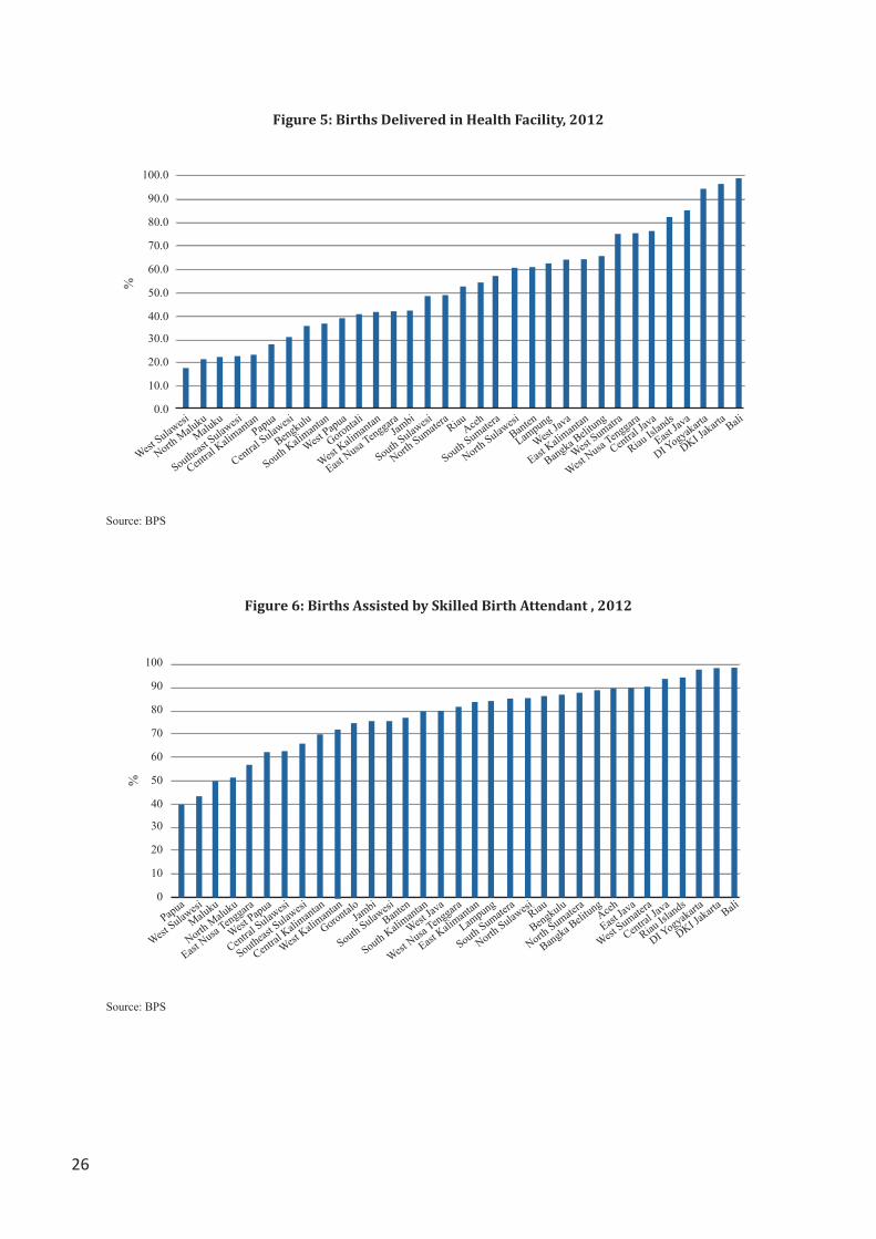
26
Figure 5: Births Delivered in Health Facility, 2012
Source: BPS
Figure 6: Births Assisted by Skilled Birth Attendant , 2012
Source: BPS
10.0
0.0
20.0
30.0
40.0
50.0
60.0
70.0
80.0
90.0
100.0
West Sulaw
esi
North M
alukuMalu
ku
Southeast S
ulawesi
Central Kalim
antanPapua
Central Sulaw
esi
Bengkulu
South Kalimantan
West Papua
Gorontali
West Kalim
antan
East Nusa T
enggaraJam
bi
South Sulawesi
North Sumate
raRiauAceh
South Sumatera
North Sulaw
esiBanten
Lampung
West Ja
va
East Kalim
antan
Bangka Belit
ung
West Sumatra
West Nusa T
enggara
Central Ja
va
Riau Isl
ands
East Ja
va
DI Yogyakarta
DKI Jakarta Bali
%
10
0
20
30
40
50
60
70
80
90
100
Papua
West Sulaw
esi
Maluku
North M
aluku
East Nusa T
enggara
West Papua
Central Sulaw
esi
Southeast S
ulawesi
Central Kalim
antan
West Kalim
antan
GorontaloJambi
South SulawesiBanten
South Kalimantan
West Ja
va
West Nusa T
enggara
East Kalim
antan
Lampung
South Sumatera
North Sulaw
esiRiau
Bengkulu
North Sumate
ra
Bangka Belit
ungAceh
East Ja
va
West Sumate
ra
Central Ja
va
Riau Isl
ands
DI Yogyakarta
DKI Jakarta Bali
%

27
Figure 7: Children Receiving Basic Vaccinations, 2012
Source: BPS
Figure 8: Urban-Rural Deprivation Composition Patterns (Censored Headcounts)
Source: BPS-Susenas 2013
0
10
20
30
40
50
60
70
80
90B
engk
ulu
Papu
aN
orth
Sum
ater
aM
aluk
uB
ante
nN
orth
Mal
uku
Wes
t Pap
uaC
entra
l Kal
iman
tan
Wes
t Sul
awes
iA
ceh
Sout
h Su
mat
era
Cen
tral S
ulaw
esi
Sout
heas
t Sul
awes
iW
est N
usa
Teng
gara
Ria
uSo
uth
Sula
wes
iR
iau
Isla
nds
Wes
t Kal
iman
tan
Sout
h K
alim
anta
nW
est S
umat
era
Lam
pung
DK
I Jak
arta
Wes
t Jav
aEa
st N
usa
Teng
gara
Jam
biG
oron
talo
Nor
th S
ulaw
esi
East
Kal
iman
tan
East
Java
Ban
gka
Bel
itung
Bal
iC
entra
l Jav
aD
I Yog
yaka
rta
%
0.000.020.040.060.080.100.120.140.160.180.20
Schooling
Enrollment
Child Mortality
Child Immunization
Skilled Birth Attendance
Electricity
Sanitation
Non-Soil Floor
Safe Drinking Water
Employed and in FormalSector
Urban Censored Headcount Rural Censored Headcount
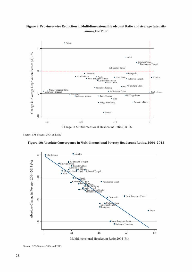
28
Figure 9: Province-wise Reduction in Multidimensional Headcount Ratio and Average Intensity among the Poor
Source: BPS-Susenas 2004 and 2013
Figure 10: Absolute Convergence in Multidimensional Poverty Headcount Ratios, 2004–2013
Source: BPS-Susenas 2004 and 2013
Aceh
Sumatera Utara
Sumatera BaratRiau
Jambi
Sumatera Selatan
Bengkulu
Lampung
Bangka Belitung
DKI Jakarta
Jawa Barat
Jawa Tengah DI Yogyakarta
Jawa Timur
Banten
BaliNusa Tenggara Barat
Nusa Tenggara Timur
Kalimantan Barat
Kalimantan Tengah
Kalimantan Selatan
Kalimantan Timur
Sulawesi Utara
Sulawesi Tengah
Sulawesi Selatan
Sulawesi Tenggara
Gorontalo
MalukuMaluku Utara
Papua
-10
-50
5
Cha
nge
in A
vera
ge D
epriv
atio
n Sc
ores
(A) -
%
-30 -20 -10 0
Change in Multidimensional Headcount Ratio (H) - %
0 20 40 60 80
Multidimensional Headcount Ratio 2004 (%)
Abs
olut
e C
hang
e in
Pov
erty
, 200
4-20
13 (%
)
Bengkulu
Bangka BelitungAceh
Sumatera UtaraSumatera Barat
Riau
Jambi
Sumatera Selatan
Lampung
DKI Jakarta
Jawa Barat
Jawa Tengah
DI Yogyakarta
Jawa TimurBanten
Bali
Nusa Tenggara Barat
Nusa Tenggara Timur
Kalimantan Barat
Kalimantan Tengah
Kalimantan Selatan
Kalimantan Timur
Sulawesi Utara
Sulawesi Tengah
Sulawesi Selatan
Sulawesi Tenggara
Gorontalo
Maluku
Maluku Utara
Papua
-30
-20
-10
0

29
Figure 11: Proportional Convergence in Multidimensional Poverty Headcount Ratios, 2004–2013
Source: BPS-Susenas 2004 and 2013
Figure 12: Absolute Convergence in Income Poverty Headcount Ratios, 2004–2013
Source: BPS-Susenas 2004 and 2013
Aceh
Sumatera Utara
Sumatera Barat
Riau
JambiBengkulu
Lampung
Bangka Belitung
DKI Jakarta
Jawa Barat
DI YogyakartaJawa Timur
Banten
BaliNusa Tenggara Barat
Nusa Tenggara TimurKalimantan Barat
Kalimantan Tengah
Kalimantan Selatan
Kalimantan Timur
Sulawesi Utara
Sulawesi Tengah
Sulawesi Selatan
Sulawesi Tenggara
Gorontalo
Maluku
Maluku Utara
Papua
Sumatera Selatan
Jawa Tengah
Multidimensional Headcount Ratio in 2004 (%)
Perc
enta
ge C
hang
e in
Pov
erty
, 200
4-20
13 (%
)
-60
-40
-20
0
0 20 40 60 80
Aceh
Sumatera Barat
Bengkulu
Bangka Belitung
DKI Jakarta
Jawa Barat
Jawa Tengah
DI Yogyakarta
Nusa Tenggara Timur
Sulawesi Utara
Sulawesi Tengah
Sulawesi Tenggara
Gorontalo
Maluku
Maluku Utara
Papua
Sumatera Utara
Sumatera Selatan
Jawa Timur
BantenBali
Nusa Tenggara Barat
Kalimantan Barat
Kalimantan Tengah
Kalimantan Selatan
Kalimantan Timur
Sulawesi SelatanRiau
Jambi
Lampung
-15
-10
-50
0 10 20 30 40
Income Poverty Headcont Ratio in 2004 (%)
Abs
olut
e C
hang
e in
Pov
erty
, 200
4-20
13 (%
)

30
Figure 13: Proportional Convergence in Income Poverty Headcount Ratios, 2004–2013
Source: BPS-Susenas 2004 and 2013
Aceh
Sumatera Utara
Sumatera Barat
Jambi
Bengkulu
Lampung
Bangka Belitung
Jawa Barat
Jawa Tengah
DI Yogyakarta
Jawa TimurBanten
Bali
Nusa Tenggara BaratNusa Tenggara Timur
Kalimantan Barat
Kalimantan Tengah
Kalimantan Selatan
Kalimantan Timur
Sulawesi Utara
Sulawesi TengahSulawesi Selatan
Sulawesi Tenggara GorontaloMaluku
Maluku Utara
Papua
Riau
Sumatera Selatan
DKI Jakarta
-60
-40
-20
020
0 10 20 30 40
Income Poverty Headcount Ratio in 2004 (%)
Perc
enta
ge C
hang
e in
Pov
erty
, 200
4-20
13 (%
)

31
Figure 14: Sensitivity of Poverty Cut-off, 2013
Source: BPS-Susenas 2013
0
0.1
0.2
0.3
0.4
0.5
0.6
0.7
0.8
0.1 0.2 0.3 0.4 0.5 0.6 0.7 0.8 0.9K
Multidimensional Headcount Ratio ( H ) - 2013
Urban Rural Indonesia
0
0.05
0.1
0.15
0.2
0.25
0.1 0.2 0.3 0.4 0.5 0.6 0.7 0.8 0.9K
Adjusted Headcount Ratio ( M0 ) - 2013
Urban Rural Indonesia
%%

32
Figure 15: Multidimensional Poverty Status by Monetary Expenditure Ranking
Source: BPS-Susenas 2013
0%
5%
10%
15%
20%
25%
30%
35%
1 2 3 4 5
Monetary Expenditure Quintiles
Multidimensional Poor (% households)
0%
5%
10%
15%
20%
25%
30%
35%
1 2 3 4 5 6 7 8 9 10Monetary Expenditure Deciles
Multidimensional Poor (% households)

33
Figure 16: Distribution of Multidimensional Poverty by Expenditure Deciles
Source: BPS-Susenas 2013
Figure 17: Distribution of Multidimensional Poverty by Expenditure Quintiles
Source: BPS-Susenas 2013
Decile 124%
Decile 217%
Decile 314%
Decile 411%
Decile 510%
Decile 68%
Decile 76%
Decile 85%
Decile 93%
Decile 101%
Deciles1 2 3 4 5 6 7 8 9 10
0% 10% 20% 30% 40% 50% 60% 70% 80% 90% 100%
Indonesia
Urban
Rural
Quintile 1 Quintile 2 Quintile 3 Quintile 4 Quintile 5
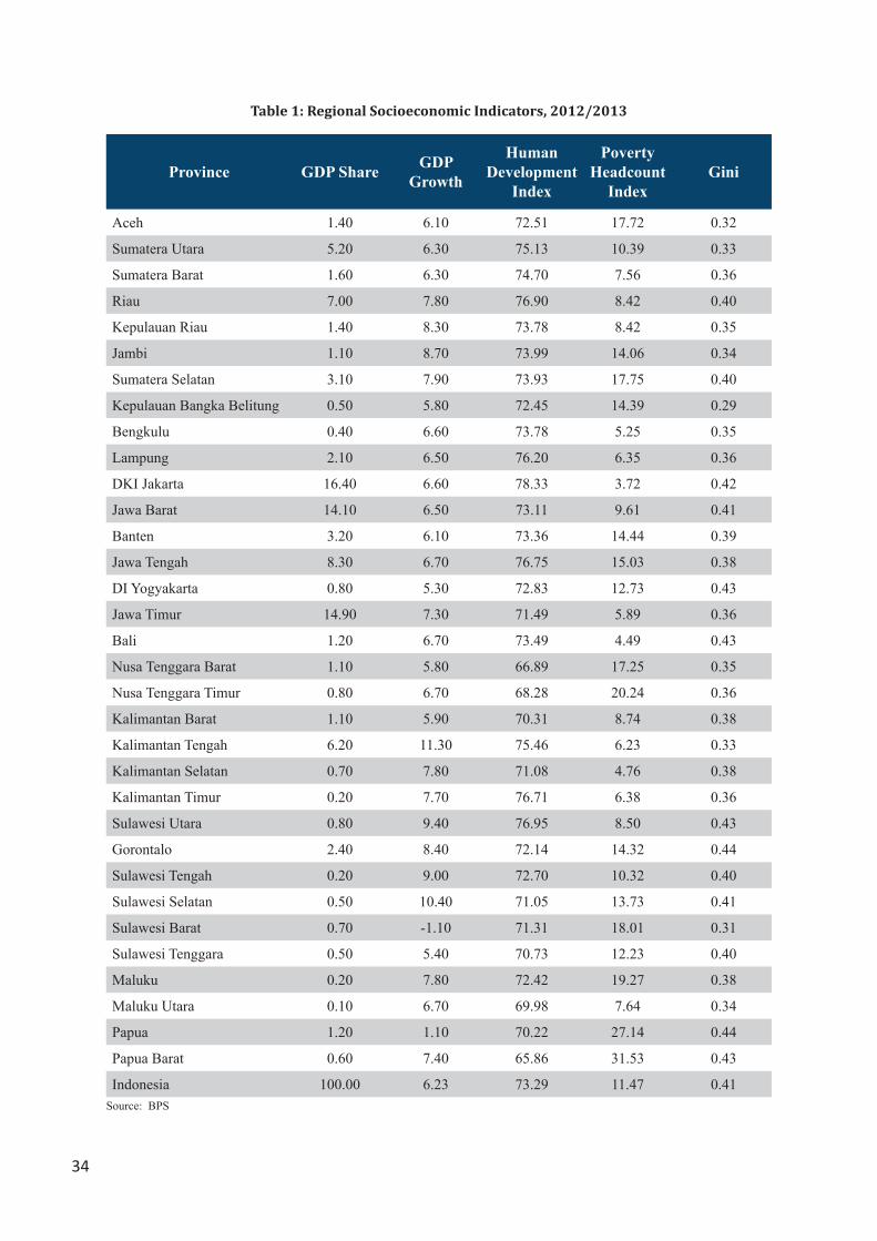
34
Table 1: Regional Socioeconomic Indicators, 2012/2013
Province GDP Share GDP Growth
Human Development
Index
Poverty Headcount
IndexGini
Aceh 1.40 6.10 72.51 17.72 0.32
Sumatera Utara 5.20 6.30 75.13 10.39 0.33
Sumatera Barat 1.60 6.30 74.70 7.56 0.36
Riau 7.00 7.80 76.90 8.42 0.40
Kepulauan Riau 1.40 8.30 73.78 8.42 0.35
Jambi 1.10 8.70 73.99 14.06 0.34
Sumatera Selatan 3.10 7.90 73.93 17.75 0.40
Kepulauan Bangka Belitung 0.50 5.80 72.45 14.39 0.29
Bengkulu 0.40 6.60 73.78 5.25 0.35
Lampung 2.10 6.50 76.20 6.35 0.36
DKI Jakarta 16.40 6.60 78.33 3.72 0.42
Jawa Barat 14.10 6.50 73.11 9.61 0.41
Banten 3.20 6.10 73.36 14.44 0.39
Jawa Tengah 8.30 6.70 76.75 15.03 0.38
DI Yogyakarta 0.80 5.30 72.83 12.73 0.43
Jawa Timur 14.90 7.30 71.49 5.89 0.36
Bali 1.20 6.70 73.49 4.49 0.43
Nusa Tenggara Barat 1.10 5.80 66.89 17.25 0.35
Nusa Tenggara Timur 0.80 6.70 68.28 20.24 0.36
Kalimantan Barat 1.10 5.90 70.31 8.74 0.38
Kalimantan Tengah 6.20 11.30 75.46 6.23 0.33
Kalimantan Selatan 0.70 7.80 71.08 4.76 0.38
Kalimantan Timur 0.20 7.70 76.71 6.38 0.36
Sulawesi Utara 0.80 9.40 76.95 8.50 0.43
Gorontalo 2.40 8.40 72.14 14.32 0.44
Sulawesi Tengah 0.20 9.00 72.70 10.32 0.40
Sulawesi Selatan 0.50 10.40 71.05 13.73 0.41
Sulawesi Barat 0.70 -1.10 71.31 18.01 0.31
Sulawesi Tenggara 0.50 5.40 70.73 12.23 0.40
Maluku 0.20 7.80 72.42 19.27 0.38
Maluku Utara 0.10 6.70 69.98 7.64 0.34
Papua 1.20 1.10 70.22 27.14 0.44
Papua Barat 0.60 7.40 65.86 31.53 0.43
Indonesia 100.00 6.23 73.29 11.47 0.41Source: BPS

35
Table 2: Dimensions, Indicators, Deprivation Cut-offs and Weights of the Multidimensional Poverty Index
Dimension Weight Indicator Weight Deprivation Cut-off
Education (1/3) Schooling (1/6) Household head has not completed elementary school
Attendance (1/6) Any school-aged child in the household is not attending school
Health (1/3) Mortality (1/9) Any child has passed away in the household
Vaccination (1/9) Any child aged 1-4 years not received measles vaccination
Birth attendance (1/9) Any child birth process not assisted by skill attendant
Standard of Living (1/3) Electricity (1/15) The household has no electricity
Sanitation (1/15) The household’s sanitation facility is not improved
Flooring material (1/15) The household has a soil floor
Water (1/15) The household does not have access to safe drinking water
Employment (1/15) Household head is unemployed or in informal labor market
Table 3: Change in Deprivations in Dimensions, 2004–2013
2004 2013Absolute Change
Percentage Change
(%)Indicators % Deprived 95% Con.Interval %
Deprived 95% Con.Interval
Schooling 0.309 0.309 0.309 0.244 0.244 0.244 -0.065 -21.014
Enrollment 0.083 0.083 0.083 0.037 0.037 0.037 -0.047 -56.002
Child Mortality 0.160 0.160 0.160 0.148 0.148 0.148 -0.012 0.000
Child Immunization 0.052 0.052 0.052 0.030 0.030 0.030 -0.022 -42.841
Skilled Birth Attendance
0.149 0.149 0.149 0.080 0.080 0.080 -0.069 -46.280
Electricity 0.130 0.130 0.130 0.037 0.037 0.037 -0.093 -71.640
Sanitation 0.552 0.552 0.552 0.363 0.363 0.363 -0.189 -34.174
Non-Soil Floor 0.145 0.145 0.145 0.075 0.075 0.075 -0.070 -48.141
Safe Drinking Water 0.224 0.224 0.224 0.148 0.148 0.148 -0.077 -34.143
Employed and in Formal Sector
0.690 0.690 0.690 0.647 0.647 0.647 -0.043 -6.210
Note: Blue shade indicates that the change is statistically significant. Following Alkire and Seth (2013), a reduction is statistically significant if the lower bound of 2004 is not lower than the upper bound of the respective 2013 estimate.
Source: BPS-Susenas 2004 and 2013

36
Table 4: Change in Multidimensional Poverty, 2004–2013
Poverty Cutoff(k)
2004 2013
Indices Values Values Absolute Change
One-third (1/3)
M(0) 0.1227 0.0603 -0.0624
H 0.2675 0.1403 -0.1272
A 0.4587 0.4298 -0.0289Source: BPS-Susenas 2004 and 2013
Table 5: Change in the Contribution of Indicators to the Overall Poverty, 2004–2013
Censored Headcount Ratio Relative Contribution
Indicator 2004 2013 Abs. Change
Perc. Change
2004 2013 Change
Schooling 0.193 0.105 -0.088 -45.39 0.262 0.291 +
Enrollment 0.069 0.025 -0.044 -64.21 0.094 0.068 -
Child Mortality 0.105 0.075 -0.031 -29.15 0.095 0.137 +
Child Immunization
0.037 0.015 -0.022 -59.95 0.033 0.027 -
Skilled Birth Attendance
0.094 0.041 -0.054 -56.94 0.085 0.075 -
Electricity 0.095 0.024 -0.071 -74.29 0.052 0.027 -
Sanitation 0.233 0.104 -0.129 -55.4 0.127 0.115 -
Non-soil Floor 0.093 0.036 -0.057 -61.1 0.05 0.04 -
Safe Drinking Water
0.127 0.06 -0.067 -52.9 0.069 0.066 -
Employed and in Formal Sector
0.244 0.139 -0.105 -42.945 0.133 0.154 +
Source: BPS-Susenas 2004 and 2013

37
Tabl
e 6:
Per
form
ance
acr
oss
Geog
raph
ic R
egio
ns, 2
004
and
2013
2004
2013
Cha
nge
Pop.
Shar
eM
0H
APo
p.Sh
are
M0
HA
M0
H
Urb
an0.
4324
90.
0408
20.
0946
60.
4312
3U
rban
0.49
822
0.02
603
0.06
486
0.40
133
-0.0
1479
-0.0
2980
Rur
al0.
5675
10.
1852
00.
3992
70.
4638
5R
ural
0.50
178
0.09
445
0.21
537
0.43
855
-0.0
9075
-0.1
8390
Prov
ince
Prov
ince
Ace
h0.
0187
60.
1073
70.
2551
00.
4208
9A
ceh
0.01
934
0.04
023
0.09
864
0.40
785
-0.0
6714
-0.1
5646
Sum
ater
a U
tara
0.05
574
0.08
500
0.18
031
0.47
141
Sum
ater
a U
tara
0.05
391
0.04
994
0.11
385
0.43
865
-0.0
3506
-0.0
6646
Sum
ater
a B
arat
0.02
067
0.10
065
0.20
201
0.49
824
Sum
ater
a B
arat
0.02
027
0.06
551
0.15
269
0.42
904
-0.0
3514
-0.0
4932
Ria
u0.
0261
50.
1284
30.
2603
70.
4932
6R
iau
0.02
462
0.06
414
0.14
858
0.43
169
-0.0
6429
-0.1
1179
Jam
bi0.
0120
60.
0958
20.
2351
10.
4075
5Ja
mbi
0.01
335
0.07
140
0.16
279
0.43
860
-0.0
2442
-0.0
7232
Sum
ater
a Se
lata
n0.
0303
60.
1364
40.
2996
70.
4553
0Su
mat
era
Sela
tan
0.03
158
0.05
765
0.13
789
0.41
809
-0.0
7879
-0.1
6178
Ben
gkul
u0.
0071
00.
1053
40.
2400
40.
4388
4B
engk
ulu
0.00
723
0.07
497
0.17
289
0.43
363
-0.0
3037
-0.0
6715
Lam
pung
0.03
234
0.19
241
0.40
489
0.47
522
Lam
pung
0.03
169
0.07
149
0.16
939
0.42
204
-0.1
2092
-0.2
3550
Ban
gka
Bel
itung
0.00
467
0.13
571
0.28
145
0.48
218
Ban
gka
Bel
itung
0.00
538
0.05
396
0.13
094
0.41
210
-0.0
8175
-0.1
5051
Kep
ulau
an R
iau
--
--
Kep
ulau
an R
iau
0.00
794
0.02
093
0.05
374
0.38
947
--
DK
I Jak
arta
0.03
983
0.00
441
0.01
070
0.41
215
DK
I Jak
arta
0.04
040
0.00
404
0.01
106
0.36
528
-0.0
0037
0.00
036
Jaw
a B
arat
0.17
715
0.09
324
0.21
245
0.43
888
Jaw
a B
arat
0.18
270
0.04
604
0.10
833
0.42
500
-0.0
4720
-0.1
0412
Jaw
a Te
ngah
0.14
936
0.13
125
0.28
361
0.46
278
Jaw
a Te
ngah
0.13
160
0.05
447
0.13
375
0.40
725
-0.0
7678
-0.1
4986
DI Y
ogya
karta
0.01
487
0.05
739
0.13
275
0.43
232
DI Y
ogya
karta
0.01
444
0.02
279
0.06
023
0.37
838
-0.0
3460
-0.0
7252
Jaw
a Ti
mur
0.16
798
0.10
978
0.25
303
0.43
386
Jaw
a Ti
mur
0.15
400
0.04
998
0.12
222
0.40
893
-0.0
5980
-0.1
3081
Ban
ten
0.04
187
0.14
973
0.30
241
0.49
512
Ban
ten
0.04
631
0.06
716
0.16
659
0.40
315
-0.0
8257
-0.1
3582

38
2004
2013
Cha
nge
Pop.
Shar
eM
0H
APo
p.Sh
are
M0
HA
M0
H
Bal
i0.
0155
70.
0547
30.
1292
50.
4234
4B
ali
0.01
664
0.01
753
0.04
507
0.38
895
-0.0
3720
-0.0
8418
Nus
a Te
ngga
ra B
arat
0.01
878
0.21
929
0.47
911
0.45
770
Nus
a Te
ngga
ra B
arat
0.01
872
0.07
432
0.17
900
0.41
520
-0.1
4497
-0.3
0011
Nus
a Te
ngga
ra T
imur
0.01
903
0.28
878
0.58
125
0.49
683
Nus
a Te
ngga
ra T
imur
0.02
009
0.18
965
0.39
497
0.48
016
-0.0
9913
-0.1
8628
Kal
iman
tan
Bar
at0.
0185
40.
2018
70.
4151
00.
4863
2K
alim
anta
n B
arat
0.01
814
0.12
976
0.29
389
0.44
153
-0.0
7211
-0.1
2121
Kal
iman
tan
Teng
ah0.
0085
90.
0747
40.
1787
50.
4181
3K
alim
anta
n Te
ngah
0.00
935
0.06
389
0.14
702
0.43
457
-0.0
1085
-0.0
3173
Kal
iman
tan
Sela
tan
0.01
483
0.13
933
0.30
576
0.45
568
Kal
iman
tan
Sela
tan
0.01
542
0.06
604
0.15
184
0.43
493
-0.0
7329
-0.1
5392
Kal
iman
tan
Tim
ur0.
0128
90.
0778
90.
1964
10.
3965
7K
alim
anta
n Ti
mur
0.01
590
0.02
888
0.07
154
0.40
369
-0.0
4901
-0.1
2487
Sula
wes
i Uta
ra0.
0099
70.
0451
00.
1101
70.
4093
7Su
law
esi U
tara
0.00
947
0.03
040
0.07
088
0.42
889
-0.0
1470
-0.0
3929
Sula
wes
i Ten
gah
0.01
030
0.14
095
0.29
693
0.47
469
Sula
wes
i Ten
gah
0.01
119
0.10
476
0.22
902
0.45
743
-0.0
3619
-0.0
6791
Sula
wes
i Sel
atan
0.03
844
0.19
381
0.40
431
0.47
936
Sula
wes
i Sel
atan
0.03
343
0.07
812
0.18
449
0.42
344
-0.1
1569
-0.2
1982
Sula
wes
i Ten
ggar
a0.
0088
10.
2469
90.
5075
70.
4866
1Su
law
esi T
engg
ara
0.00
952
0.08
628
0.19
532
0.44
174
-0.1
6071
-0.3
1225
Gor
onta
lo0.
0041
10.
2124
00.
4589
10.
4628
4G
oron
talo
0.00
445
0.12
216
0.26
701
0.45
751
-0.0
9024
-0.1
9190
Sula
wes
i Bar
at-
--
-Su
law
esi B
arat
0.00
507
0.15
993
0.34
401
0.46
490
--
Mal
uku
0.00
570
0.10
110
0.21
213
0.47
659
Mal
uku
0.00
669
0.10
038
0.21
715
0.46
226
-0.0
0072
0.00
502
Mal
uku
Uta
ra0.
0039
80.
2078
40.
4406
90.
4716
2M
aluk
u U
tara
0.00
450
0.10
189
0.22
172
0.45
954
-0.1
0595
-0.2
1897
Papu
a B
arat
--
--
Papu
a B
arat
0.00
340
0.06
935
0.15
829
0.43
812
--
Papu
a0.
0115
60.
3527
20.
7539
20.
4678
5Pa
pua
0.01
323
0.26
660
0.50
279
0.53
024
-0.0
8612
-0.2
5113
Indo
nesi
a1.
0000
00.
1227
60.
2675
30.
4588
6In
done
sia
1.00
000
0.06
036
0.14
038
0.42
998
-0.0
6240
-0.1
2715
Sour
ce: B
PS-S
usen
as 2
004
and
2013
Tabl
e 6:
Per
form
ance
acr
oss
Geog
raph
ic R
egio
ns, 2
004
and
2013
(Con
tinu
ed)

39
Tabl
e 7:
Per
form
ance
by
Hou
seho
ld C
hara
cter
isti
cs, 2
004
and
2013
2004
2013
Cha
nge
Pop.
Shar
eH
MA
Pop.
Shar
eH
MA
MH
Mal
e 0.
903
0.26
70.
123
0.46
20.
896
0.13
90.
060
0.43
2-0
.064
-0.1
29
Fem
ale
0.09
70.
270
0.11
60.
430
0.10
40.
155
0.06
40.
417
-0.0
52-0
.115
Age
29
and
Less
0.06
80.
210
0.09
40.
448
0.07
60.
091
0.04
00.
441
-0.0
54-0
.119
Age
30-
590.
756
0.24
80.
116
0.46
70.
774
0.12
50.
055
0.43
6-0
.061
-0.1
23
Age
60
and
Plus
0.17
60.
374
0.16
40.
438
0.15
00.
245
0.10
10.
412
-0.0
63-0
.130
Hou
seho
ld si
ze <
=40.
512
0.23
50.
102
0.43
40.
537
0.11
00.
046
0.41
5-0
.056
-0.1
25
Hou
seho
ld si
ze>=
50.
488
0.30
20.
145
0.47
90.
463
0.17
60.
077
0.44
0-0
.067
-0.1
26So
urce
: BPS
-Sus
enas
200
4 an
d 20
13

40
Table 8: Income Poverty vs. Multidimensional Poverty MatrixC
onsu
mpt
ion
Multidimensional
Non-Poor Poor Total
Non-Poor 78.29 10.35 88.63
Poor 7.67 3.69 11.37
Total 85.96 14.04 100
Source: BPS-Susenas 2013
Table 9: Income Poverty vs. Multidimensional Poverty – Conditional Probability Matrix (given income poverty)
Con
sum
ptio
n
Multidimensional
Non-Poor Poor Total
Non-Poor 0.88 0.12 88.63
Poor 0.67 0.32 11.37
Total 85.96 14.04 100
Source: BPS-Susenas 2013
Table 10: Lack of Overlap between Income and Multidimensional Poverty
% of Population K=1 K=2 K=3 K=4 K=5
Income non-poor, but multidimensionally poor 45.83 28.43 10.35 5.45 1.46
Income poor, but multidimensionally non-poor 1.93 3.92 7.67 8.81 10.31
Source: BPS-Susenas 2013

41
Table 11: Kendall Tau b Coefficient between Income and Multidimensional Poverty Index Indicators
Income
Schooling 0.1497
Enrollment 0.1102
Child Mortality -0.0677
Child Immunization 0.0605
Skilled Birth Attendance 0.1401
Electricity 0.1384
Sanitation 0.1849
Non-Soil Floor 0.128
Safe Drinking Water 0.1141
Employment and Informal Sector 0.1349Source: BPS-Susenas 2013

42
TNP2K Working Paper Series
Title Author(s) Date Published Keywords
Working Paper 1
Finding the Best Indicators to Identify the Poor
Adama Bah September 2013 Proxy-Means Testing, Variable/Model Selection, Targeting, Poverty, Social Protection
Working Paper 2
Estimating Vulnerability to Poverty using Panel Data: Evidence from Indonesia
Adama Bah October 2013 Poverty, Vulnerability, Household consumption
Working Paper 3
Education Transfer, Expenditures and Child Labour Supply in Indonesia: An Evaluation of Impacts and Flypaper Effects
Sudarno Sumarto, Indunil De Silva
December 2013 Cash transfers, child labour, education expenditure, flypaper effect
Working Paper 4
Poverty-Growth-Inequality Triangle: The Case of Indonesia
Sudarno Sumarto, Indunil De Silva
December 2013 Growth, poverty, inequality, pro-poor, decomposition
Working Paper 5
English version:Social Assistance for the Elderly in Indonesia: An Empirical Assessment of the Asistensi Sosial Lanjut Usia Terlantar Programme*
Bahasa Indonesia version:Asistensi Sosial untuk Usia Lanjut di Indonesia: Kajian Empiris Program Asistensi Sosial Lanjut Usia Terlantar*
Sri Moertiningsih Adioetomo, Fiona Howell, Andrea McPherson, Jan Priebe
March 2013
*This Working Paper has been republished in 2014
ASLUT Programme, Elderly, Social Pensions, Lanjut Usia, Social Assistance, Social Security, Indonesia
Working Paper 6
An Evaluation of the Use of the Unified Database for Social Protection Programmes by Local Governments in Indonesia
Adama Bah, Fransiska E. Mardianingsih, Laura Wijaya
March 2014 Unified Database, UDB, Basis Data Terpadu, BDT, Local Governments Institution
Working Paper 7
Old-Age Poverty in Indonesia: Empirical Evidence and Policy Options - A Role for Social Pensions
Jan Priebe, Fiona Howell
March 2014 Social Pensions, Old-Age, Poverty, Elderly, ASLUT Programme, Indonesia
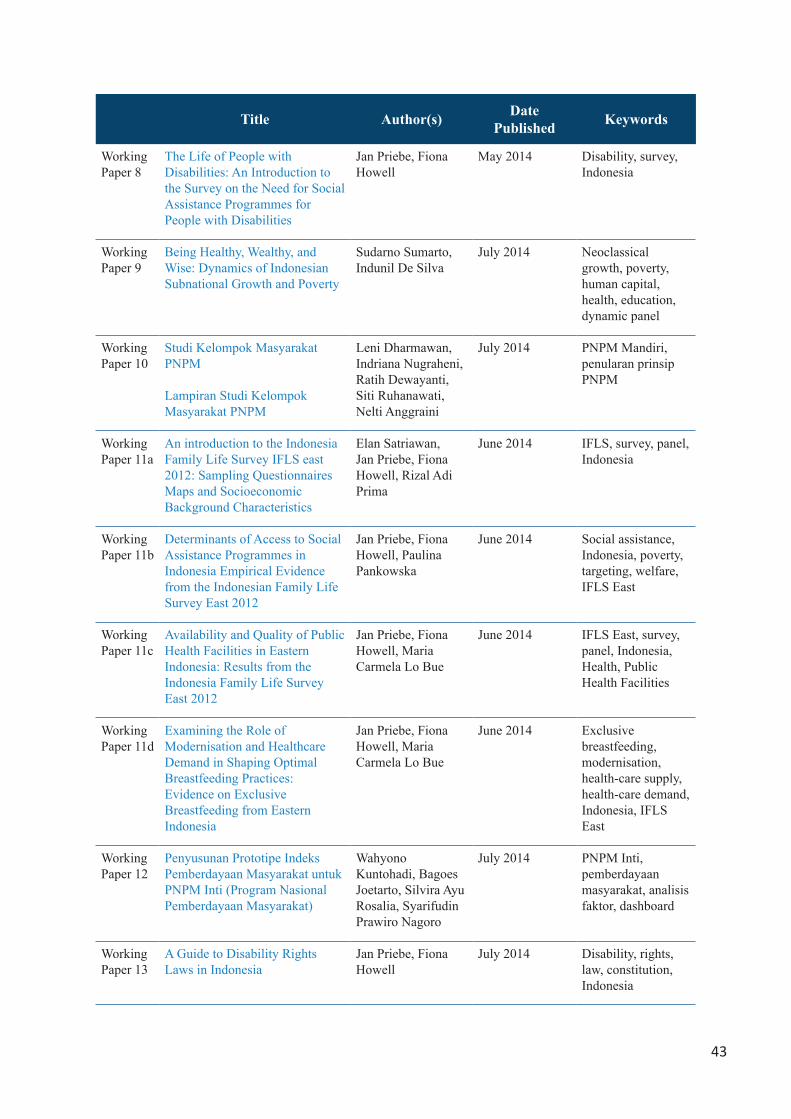
43
Title Author(s) Date Published Keywords
Working Paper 8
The Life of People with Disabilities: An Introduction to the Survey on the Need for Social Assistance Programmes for People with Disabilities
Jan Priebe, Fiona Howell
May 2014 Disability, survey, Indonesia
Working Paper 9
Being Healthy, Wealthy, and Wise: Dynamics of Indonesian Subnational Growth and Poverty
Sudarno Sumarto, Indunil De Silva
July 2014 Neoclassical growth, poverty, human capital, health, education, dynamic panel
Working Paper 10
Studi Kelompok Masyarakat PNPM
Lampiran Studi Kelompok Masyarakat PNPM
Leni Dharmawan, Indriana Nugraheni, Ratih Dewayanti, Siti Ruhanawati, Nelti Anggraini
July 2014 PNPM Mandiri, penularan prinsip PNPM
Working Paper 11a
An introduction to the Indonesia Family Life Survey IFLS east 2012: Sampling Questionnaires Maps and Socioeconomic Background Characteristics
Elan Satriawan, Jan Priebe, Fiona Howell, Rizal Adi Prima
June 2014 IFLS, survey, panel, Indonesia
Working Paper 11b
Determinants of Access to Social Assistance Programmes in Indonesia Empirical Evidence from the Indonesian Family Life Survey East 2012
Jan Priebe, Fiona Howell, Paulina Pankowska
June 2014 Social assistance, Indonesia, poverty, targeting, welfare, IFLS East
Working Paper 11c
Availability and Quality of Public Health Facilities in Eastern Indonesia: Results from the Indonesia Family Life Survey East 2012
Jan Priebe, Fiona Howell, Maria Carmela Lo Bue
June 2014 IFLS East, survey, panel, Indonesia, Health, Public Health Facilities
Working Paper 11d
Examining the Role of Modernisation and Healthcare Demand in Shaping OptimalBreastfeeding Practices: Evidence on Exclusive Breastfeeding from EasternIndonesia
Jan Priebe, Fiona Howell, Maria Carmela Lo Bue
June 2014 Exclusive breastfeeding, modernisation, health-care supply, health-care demand, Indonesia, IFLS East
Working Paper 12
Penyusunan Prototipe Indeks Pemberdayaan Masyarakat untuk PNPM Inti (Program Nasional Pemberdayaan Masyarakat)
Wahyono Kuntohadi, Bagoes Joetarto, Silvira Ayu Rosalia, Syarifudin Prawiro Nagoro
July 2014 PNPM Inti, pemberdayaan masyarakat, analisis faktor, dashboard
Working Paper 13
A Guide to Disability Rights Laws in Indonesia
Jan Priebe, Fiona Howell
July 2014 Disability, rights, law, constitution, Indonesia

44
Title Author(s) Date Published Keywords
Working Paper 14
Social Assistance for the Elderly: The Role of the Asistensi Sosial Lanjut Usia Terlantar Programme in Fighting Old Age Poverty
Sri Moertiningsih Adioetomo, Fiona Howell, Andrea Mcpherson, Jan Priebe
August 2014 ASLUT Programme, Social Assistance, Elderly, Poverty, Indonesia
Working Paper 15
Productivity Measures for Health and Education Sectors in Indonesia
Menno Pradhan, Robert Sparrow
September 2014 Health, Education, Productivity Measures, Spending, Expenditure, Indonesia
Working Paper 16
Demand for Mobile Money and Branchless Banking amongMicro and Small Enterprises in Indonesia
Guy Stuart, Michael Joyce, Jeffrey Bahar
September 2014 Micro and small enterprises, MSEs, Mobile Money, Branchless Banking, Financial Services, Indonesia
Working Paper 17
Poverty and the Labour Market in Indonesia: Employment Trends Across the Wealth Distribution
Jan Priebe, Fiona Howell, Virgi Agita Sari
October 2014 Labour, Employment, Working Poor, Poverty, Wealth Distribution, Indonesia
Working Paper 18
PNPM Rural Income Inequality and Growth Impact Simulation
Jon R. Jellema October 2014 PNPM Rural, Income, Income Inequality, Infrastucture
Working Paper 19a
Youth Employment in Indonesia:International and National Good Practices for Policy and Programme Improvement
Léa Moubayed, R. Muhamad Purnagunawan
December 2014 Youth Employment, Education, Vocational, Labour, Training
Working Paper 19b
Youth Employment in Indonesia: Compendium of Best Practices and Recommendations for Indonesia
Léa Moubayed,R. MuhamadPurnagunawan
December 2014 Youth Employment, Education, Vocational, Labour, Training, Good Practices
Working Paper 20
Finding the Poor vs. Measuring Their Poverty: Exploring the Drivers of Targeting Effectiveness in Indonesia
Adama Bah, Samuel Bazzi, Sudarno Sumarto, and Julia Tobias
November 2014 Targeting, Proxy-Means Testing, Social Protection, Poverty

45

46


SEKRETARIATTIM NASIONAL PERCEPATAN PENANGGULANGAN KEMISKINAN
Grand Kebon Sirih Lt. 4Jl. Kebon Sirih Raya No. 35 Jakarta Pusat 10110, IndonesiaTelp : 021 - 3912 812Faks : 021 - 3912 511Website : www.tnp2k.go.id
The aim of this study was twofold. First, although a number of empirical studies exist on income poverty in Indonesia, very few have examined multidimensional household welfare deprivations. We attempted to fill this gap by using for the first time the annually conducted National Socioeconomic Survey by Statistics Indonesia (BPS), and the Alkire and Foster (2007; 2011) methodology to investigate the degree and dynamics of multidimensional household welfare deprivations in Indonesia for the 2004 and 2013 time periods. Second, we explore whether there are differing patterns of change for consumption poverty and multidimensional poverty at both the household and regional level. We investigate the magnitude of overlap between consumption and multidimensional poverty, and explore whether the multidimensionally deprived households are necessarily income poor or not and vice versa. In particular we scrutinize whether the question of who is poor has many different answers.
This paper is innovative in that it changes the focus from the conventional unidimensional perspective of poverty, centered on income or expenditure to a much broader multidimensional approach. Our results revealed the overlap between consumption poverty and multidimensional poverty to be extremely weak. Our findings broaden the targeting space for poverty reduction, suggesting that poverty reduction programmes should provide different kinds of assistance to the poor in different dimensions of poverty. Results clearly demonstrate the question of who is poor to have many different answers. So overall, the findings from the study underscore the need to use both monetary and multidimensional poverty indices to understand the extent, diversity and dynamics of household welfare in Indonesia. Thus placing policy analytics on fundamentally important capability deprivations, rather than only on a convenient proxy such as income or consumption will not only help to better comprehend poverty and deprivation – but also to combat them.
TIM NASIONAL PERCEPATAN PENANGGULANGAN KEMISKINAN(TNP2K)
Jl. Kebon Sirih No. 35, Jakarta Pusat 10110Tel: +62 (0) 21 391 2812Fax: +62 (0) 21 391 2511E-mail: [email protected] Web: www.tnp2k.go.id
7513117860229
ISBN 9786022751311