Journal of Applied Geophysics 98 (2013) 160–175

Contents lists available at ScienceDirect

Journal of Applied Geophysics

j ourna l homepage: www.e lsev ie r .com/ locate / j appgeo

An implementation of differential evolution algorithm for inversion ofgeoelectrical data

Çağlayan Balkaya ⁎Süleyman Demirel University, Engineering Faculty, Department of Geophysical Engineering, West Campus, 32260 Isparta, Turkey

⁎ Tel.: +90 246 2111360.E-mail address: caglayanbalkaya@sdu.edu.tr.

0926-9851/$ – see front matter © 2013 Elsevier B.V. All rihttp://dx.doi.org/10.1016/j.jappgeo.2013.08.019

a b s t r a c t

a r t i c l e i n f o

Article history:Received 7 November 2012Accepted 31 August 2013Available online 8 September 2013

Keywords:Differential evolution (DE)Evolutionary algorithm (EA)Global optimizationGeoelectrical methodsMetropolis–Hastings sampling

Differential evolution (DE), a population-based evolutionary algorithm(EA) has been implemented to invert self-potential (SP) and vertical electrical sounding (VES) data sets. The algorithm uses three operators includingmu-tation, crossover and selection similar to genetic algorithm (GA).Mutation is themost important operator for thesuccess of DE. Three commonly usedmutation strategies including DE/best/1 (strategy 1), DE/rand/1 (strategy 2)and DE/rand-to-best/1 (strategy 3) were applied together with a binomial type crossover. Evolution cycle of DEwas realizedwithout boundary constraints. For the test studies performedwith SP data, in addition to both noise-free and noisy synthetic data sets two field data sets observed over the sulfide ore body in the Malachite mine(Colorado) and over the ore bodies in the Neem-Ka Thana cooper belt (India) were considered. VES test studieswere carried out using synthetically produced resistivity data representing a three-layered earth model and afield data set example from Gökçeada (Turkey), which displays a seawater infiltration problem. Mutation strat-egies mentioned above were also extensively tested on both synthetic and field data sets in consideration. Ofthese, strategy 1was found to be themost effective strategy for the parameter estimation by providing less com-putational cost together with a good accuracy. The solutions obtained by DE for the synthetic cases of SP werequite consistent with particle swarm optimization (PSO) which is a more widely used population-based optimi-zation algorithm than DE in geophysics. Estimated parameters of SP and VES datawere also comparedwith thoseobtained from Metropolis–Hastings (M–H) sampling algorithm based on simulated annealing (SA) withoutcooling to clarify uncertainties in the solutions. Comparison to the M–H algorithm shows that DE performs afast approximate posterior sampling for the case of low-dimensional inverse geophysical problems.

© 2013 Elsevier B.V. All rights reserved.

1. Introduction

Geoelectrical methods including self-potential (SP) and direct current(DC) electrical resistivity based on vertical electrical sounding (VES) tech-nique are widely used for a wide variety of exploration problems such asmineral explorations (e.g., Meiser, 1962; Yüngül, 1950, 1954), land-slides (e.g., Bogoslovsky and Ogilvy, 1977), environmental problems(Bolève et al., 2011; Park et al., 2007), groundwater investigations(e.g., Göktürkler et al., 2008; Hamzah et al., 2007), geothermal ex-plorations (e.g., Drahor and Berge, 2006; Özurlan et al., 2006), cavedetection (e.g., Balkaya et al., 2012; Vichabian and Morgan, 2002) andarchaeological prospection (e.g., Drahor, 2004; El-Qady et al., 1999).

Model parameters of SP and VES anomalies may be estimated byeither local or global optimization methods that have both advantagesand disadvantages relative to each other. Converging to the best-fitting solutionusing traditional gradient-based local-search optimizationalgorithms strongly depend on a good initial guess, while computational-ly expensive global-search algorithmsusing nature-inspired evolutionary

ghts reserved.

algorithms (EAs) are not sensitive to the choice of the initial model(Başokur et al., 2007; Chunduru et al., 1997; Göktürkler, 2011). These al-gorithms as a sampler do not require a prior model. The only prior infor-mation for EAs is the search space,which can be enlarged especially in thepresence of noisy data. Thus, they may be preferable to the local onessince prior information is not generally known (Fernández-Martínezet al., 2010b). Commonly used global optimization algorithms, whichare based on direct search, include genetic algorithm (GA) (Holland,1975), particle swarm optimization (PSO) (Kennedy and Eberhart,1995) and simulated annealing (SA) (Kirkpatrick et al., 1983). GA(Abdelazeem and Gobashy, 2006), PSO (Monteiro Santos, 2010; Pekşenet al., 2011) and adaptive SA (ASA) (Tlas and Asfahani, 2008) wereused for the interpretation of SP anomalies. Göktürkler and Balkaya(2012) performed a comparative study for these three algorithms to in-vert single SP anomalies caused by somepolarized bodieswith simple ge-ometries. Additionally, GA (Balkaya et al., 2012; Fernández Alvarez et al.,2008; Jha et al., 2008), PSO (Fernández Martinez et al., 2010a; Shaw andSrivastava, 2007) and SA (Dittmer and Szymanski, 1995; Sen et al., 1993)were applied to invert VES data. Hybrid approaches combining local andglobal optimization algorithms were also used by researchers. For in-stance, Chunduru et al. (1997) used combined local conjugate gradient(CG) and global very fast SA (VFSA), and Başokur et al. (2007) used GA

161Ç. Balkaya / Journal of Applied Geophysics 98 (2013) 160–175

both as a stand-alone and as a hybrid approach together with iterativedamped least-squares, namely Lamarckian inversion.

Differential evolution algorithm (DE), a class of EAs, was introducedby Storn and Price (1995) for solving a polynomial fitting problem.The algorithm is generally called as a very simple but very powerfulpopulation-based meta-heuristic algorithm (e.g., Qing, 2009, p. 41).DE is based on adding a weighted difference between two randomlychosen individuals from the population to a third one to find out newindividuals in every generation (Storn and Price, 1997). It is similarto GA that is the most popular EA since DE uses the same genetic oper-ators for optimization. But, DE uses these operators in a different order(mutation, crossover and selection) from GA (crossover, mutation andselection) in the reproduction cycle. In DE, mutation is carried outbefore crossover. DE includes ten different strategies: five differentmutation implementations and two crossover operators (binomialand exponential) for each of them. The algorithm is generally char-acterized by the features of simplicity, effectiveness and robustness.Also, it is easy-to-use; and it requires few controlling parameters, and ithas fast convergence characteristic (e.g., Noman et al., 2011; Storn andPrice, 1997). Due to these advantages, it presents awide range of imple-mentation examples in different areas such as acoustics, biology, mate-rial science, mechanic, medical imaging, optic, mathematics, physics,seismology, etc. More details and examples about the implementationof DE to solve various problems are given in Qing (2009, pp. 41–51).Even though previous comprehensive studies over both commonbenchmark functions and real-world problems have shown that DEperforms better in terms of convergence rate and robustness than theother EAs mentioned above, it has a very limited implementation ingeophysical data inversion. DE has been used in geophysics for kinematiclocation of earthquake hypocenter (Růžek and Kvasnička, 2001); inver-sion of well-log data (Goswami et al., 2004); stochastic inversion ofpost-stack seismic data (Saraswat et al., 2010). Recently, Balkaya andGöktürkler (2012) and Li and Yin (2012) used DE for quantitative inter-pretation of self-potential data.

This study aimed to assess implementation of DE for inversion ofgeoelectrical data obtained by SP and VES studies. Threemost frequent-ly usedmutation strategies with the binomial crossover typewere usedin the algorithm. Synthetically produced (i.e., noise-free and noisy) andtwo field data sets were considered in the SP implementation. Twoknown anomalies obtained over a Malachite mine (Jefferson County,Colorado) and over the ore bodies in the Neem-Ka-Thana, Rajasthancooper belt (India) were used in the test studies. The solutions gen-erated by DE were also compared with the results obtained by PSOthat has been widely used to tackle geophysical inverse problems.Classical implementations of both algorithmswere used in the compar-ison. The VES implementation includes interpretation of a three-layeredsynthetic resistivity curve and an example of a field data set fromGökçeada, Turkey. To clarify uncertainties in the solutions, modelparameters from SP anomalies (electric dipole moment, polarizationangle, depth, shape factor and origin of the anomaly) and VES curves(resistivity and thickness of the layers) were compared with the resultsfromMetropolis–Hastings (M–H) sampling algorithmusing SAwithouta cooling schedule. Comparison to theM–H algorithm indicates that DEperforms a fast approximate posterior sampling for the case of low-dimensional inverse geophysical problems. As a result, DE can be con-sidered as an effective algorithm by yielding compatible solutionswith PSO in the inverse geoelectrical problems.

2. DE algorithm

DE algorithm (Price et al., 2005; Storn, 2008, pp. 1–31; Storn andPrice, 1995) is one of the population-based global optimization algo-rithms having common sequence steps of an EA. Similar to GA; thealgorithm has two stages including initialization and evolution.After randomly generating initial population by initialization, popu-lation evolves from one generation to the next through mutation,

crossover and selection operations until the termination criteria arereached (Lin et al., 2011). One of the main differences between DE andGA is that the reproduction is carried out by a differentialmutation beforethe crossover. Reproduction cycle to generate individuals for the nextgeneration is carried out by basic operations of DE as described in thefollowing sections.

2.1. Initialization

The algorithm begins by creating an initial population of targetvectors consisting of parameters xi,G = (xi,G1 , …,xi,GD ), i = (1, …,Np)where Np is the population size, D is the number of parameters, G de-notes the current generation, that is iteration in algorithm, and i is theindex for individuals. The algorithm is initialized by a randomly createdpopulation within a predefined search space considering the upper andlower bounds of each parameter as follows:

xji;G ¼ xj

l þ rand 0;1ð Þ � xju−xj

l

� �; j ¼ 1;2;…;D ð1Þ

where j indicates parameters, l and u indicate lower and upper param-eter bounds, respectively, and rand() represents a uniformly distributedrandom variable in the range of [0,1).

2.2. Mutation operation

This operation is performed after the initialization to create amutant(donor) vector vi,G = (vi,G1 ,vi,G2 , …,vi,GD ) for each target vector. Table 1shows the most common mutation schemes used in DE. Consideringthe classical approach in DE (the second strategy: DE/rand/1), three dif-ferent vectors consisting of a base vector (xr1) and twodifference vectors(xr2 and xr3 ) are randomly chosen from the population. Mutation oper-ation is then carried out by perturbing the base vector via a differencevector scaled by a weighting factor F (mutation constant).

In Table 1, xbest,G is the best individual vector in the population atgeneration G, and indexes are random and mutually exclusive integers,and none of them corresponds to the base index i of current targetvector. In order to describe different types of mutation schemes givenin Table 1, a unique notation is generally used: DE/x/y/z, where x indi-cates how the base vector chosen (rand: vector is randomly selectedand best: vector with the lowest objective function value), y indicateshow many difference vector is added to it and z indicates what type ofcrossover method is chosen (i.e., binomial (bin) or exponential (exp))(Price et al., 2005, p. 47).

2.3. Crossover operation

The trial vector is created bymeans of crossover operation oncemu-tation operation has been terminated. It is realized between each pair oftarget vector (xi,G) and its corresponding mutant vector (vi,G), and canbe simply formulated for the binomial uniform crossover that is widelyused in the literature as shown below.

uji;G ¼ vj

i;G if rand 0;1ð Þ≤Cr or j ¼ jrandð Þ;xji;G otherwise;

j ¼ 1;2;…;D

(ð2Þ

where Cr is a user-defined crossover probability in the range [0, 1],which controls the fraction of parameter values copied from themutantvector, and jrand is a randomly chosen integer in the range [1, D] toprovide that the trial vector does not duplicate the target vector(Mandal et al., 2011; Price et al., 2005, p. 40).

Table 1The five mostly used mutation schemes applied in the classical DE.

Strategy Description Mutation schemes

1 DE/best/1 vi;G ¼ xbest;G þ F � xri1 ;G−xri2 ;G� �

2 DE/rand/1 vi;G ¼ xri1 ;G þ F � xri2 ;G−xri3 ;G� �

3 DE/rand-to- best/1 vi;G ¼ xri1 ;G þ F � xbest;G−xri2 ;G� �

þ F � xri3 ;G−xri4 ;G� �

4 DE/best/2 vi;G ¼ xbest;G þ F � xri1 ;G−xri2 ;G� �

þ F � xri3 ;G−xri4 ;G� �

5 DE/rand/2 vi;G ¼ xri1 ;G þ F � xri2 ;G−xri3 ;G� �

þ F � xri4 ;G−xri5 ;G� �

162 Ç. Balkaya / Journal of Applied Geophysics 98 (2013) 160–175

2.4. Selection operation

The last operation of DE, selection is achieved from the target andtrial vectors by comparing their objective function values (misfit)through a condition given below.

xi;Gþ1 ¼ ui;G if f ui;G

� �≤ f xi;G

� �xi;G otherwise:

(ð3Þ

In the current population, target vector is updated when the newlygenerated trial vector provides equal or lower misfit value than that ofits target vector. There is no boundary constraints for trial parametersthat exceed initial upper and lower bounds of each parameter. This evo-lution cyclementioned above is repeated until a termination criterion isreached (e.g., number of generations reaches a preset maximum num-ber of populations or the best objective function value is not improved

Fig. 1. The pseudocode for strategy 1 (DE/best/1/bin).Adopted from Mezura-Montes and Palomeque-Ortiz (2009).

considering a threshold value that is defined as value to reach (VTR) inDE). Fig. 1 shows a pseudocode of DE algorithm for the first strategy(i.e., DE/best/1/bin), where the base vector is chosen to be best vectorof the current generation and there is only a pair of differential vectorsand a binomial crossover is used.

2.5. Control parameters of DE algorithm

DE includes three control parameters, which areNp, F and Cr. Choos-ing the proper control parameter values in DE may be a crucial andtime-consuming task because this affects the performance of the algo-rithm. To overcome it, researchers have developed some schemes that

Fig. 2. Three superimposed synthetic SP anomalies (top) caused by a semi-infinite verticalcylinder (q = 0.5), an infinitely long horizontal cylinder (q = 1) and a sphere (q = 1.5)with a cross-sectional views of the bodies and parameters (middle), and rs and rc denoteradius of corresponding bodies. Explanations for model parameters of each body arealso given in the bottom of the figure.

Fig. 3. (a–h) Error maps in the vicinity of each pair of SP parameters for noise-free data.

163Ç. Balkaya / Journal of Applied Geophysics 98 (2013) 160–175

are capable of employing self-adaptive parameter control techniquesparticularly for F and Cr (e.g., Brest et al., 2006). Suggestions for controlparameter settings fromprevious studiesmay also beused. For instance,the value of Np is suggested to be multiple times of D, generally rangingfrom 3D to 20D. Its setting above an optimal value does not improve thesolution (e.g., Lin et al., 2011) butmay greatly increase computing time.Adequate value of Cr rangingwithin [0, 1] and affecting the convergencerate depends on the problem to be solved (i.e., Gämperle et al., 2002).For instance, Cr ≤ 0.2 is suitable for the separable functions while

Table 2Optimization results of noise-free synthetic data set by DE using strategy 1 for variousvalues of F and Cr. In the table, the upper and lower numbers represent the means NGand the success rates inNp of 100, respectively. Of these, F = 0.5 and Cr = 0.9 that appearin bold face type greatly accelerate the convergence speed of DE algorithm.

Cr F

0.1 0.2 0.3 0.4 0.5 0.6 0.7 0.8 0.9

0.1 299.0 300.0 300.0 300.0 300.0 300.0 300.0 300.0 300.00.07 0.0 0.0 0.0 0.0 0.0 0.00 0.0 0.0

0.2 298.7 295.0 300.0 300.0 300.0 300.0 300.0 300.0 300.00.03 0.07 0.0 0.0 0.0 0.0 0.0 0.0 0.0

0.3 286.7 267.5 273.4 293.8 300.0 300.0 300.0 300.0 300.00.3 0.37 0.3 0.13 0.0 0.0 0.0 0.0 0.0

0.4 201.3 174.0 184.0 227.8 276.2 296.3 300.0 300.0 300.00.87 1.0 0.97 0.93 0.67 0.07 0.0 0.0 0.0

0.5 109.4 113.3 111.2 131.6 172.7 241.3 299.3 300.0 300.01.0 1.0 1.0 1.0 1.0 1.0 0.13 0.0 0.0

0.6 64.4 109.1 72.0 84.9 111.5 158.8 219.7 291.2 300.01.0 1.0 1.0 1.0 1.0 1.0 1.0 0.37 0.0

0.7 48.6 85.0 54.8 61.0 78.03 107.9 160.2 218.8 299.31.0 1.0 1.0 1.0 1.0 1.0 1.0 1.0 0.1

0.8 35.9 56.4 76.7 43.9 54.17 79.0 113.1 166.5 240.81.0 1.0 1.0 1.0 1.0 1.0 1.0 1.0 1.0

0.9 26.1 37.6 51.6 53.2 41.4 57.2 86.07 126.6 189.61.0 1.0 1.0 1.0 1.0 1.0 1.0 1.0 1.0

Cr ≥ 0.9 is suitable for the non-separable ones (i.e., Rönkkönen et al.,2005). Similarly, Price et al. (2005, p. 100, 101) emphasize that Crshould be close to 1 for parameter dependent functions to prevent per-formance losses originated from low mutation rate. The scale factor (F)ranging within [0, 2] is usually taken as less than 1. It must be abovegreater than a certain value because small values may get trapped ina local minimum while large values may reduce convergence rate(Rönkkönen et al., 2005; Zaharie, 2009). Storn and Price (1997) report-ed that 0.5 is a good initial choice for the scale factor, and Rönkkönenet al. (2005) suggested that it should be set in the range [0.4, 0.95]. Onthe other hand, randomizations of F, i.e., dither and jitter (e.g., Priceet al., 2005, pp. 80–87; Storn, 2008, pp.11–12), or time-varying scalefactor mechanisms yielding good results are also proposed (e.g., Daset al., 2005). As it is stated on the homepage of DE (http://www1.icsi.berkeley.edu/~storn/code.html), dither based on selecting F randomlyfor each generation (see Eq. (4)) or for each difference vector (seeEq. (5)) is significantly useful for improving convergence behavior ofDE, especially in the case of noisy objective functions. Jitter (see Eq. (6))based on randomizing the difference vector in all parameter directions

Table 3The best solution of 30 independent runs by using three strategies of DE algorithm fornoise-free data set.

Strategy Variant G K(mV · m2q−1)

θ (°) z0(m)

q x0(m)

rms(mV)

1 Classic 37 −1000.16 30.00 5.00 1.00 40.00 0.0035With jitter 58 −1000.19 29.99 5.00 1.00 40.00 0.0057

2 Classic 91 −1000.32 29.98 5.00 1.00 40.00 0.0083With per-vector-dither

194 −999.50 30.01 5.00 1.00 40.00 0.0081

With per-G-dither

185 −1000.42 30.00 5.00 1.00 40.00 0.0088

3 Classic 75 −999.76 30.00 5.00 1.00 40.00 0.0023

Table 4Comparison of statistics of DE obtained by each strategy for noise-free data set.

Strategy 1 Strategy 2 Strategy 3

Classic With jitter Classic With-per-vector-dither With per-G-dither

Successes 30/30 30/30 30/30 30/30 30/30 30/30Mean NG 45.63 43.00 136.13 195.90 188.43 65.63SD G 15.91 15.40 39.25 24.10 20.36 18.44Mean NFE 4563.33 4300.00 13613.33 19590.00 18843.33 6563.33SD NFE 1590.59 1539.59 3924.96 2409.94 2035.66 1843.81SD rms (mV) 0.043 0.44 0.77 0.022 0.038 0.45Mean rms (mV) 0.036 0.11 1.36 0.029 0.042 0.13Min. rms (mV) 0.0035 0.0057 0.0083 0.0081 0.0088 0.0023Solutiona (s) 1.86 2.26 7.02 9.99 9.69 3.43

a Average CPU time for each independent runs.

164 Ç. Balkaya / Journal of Applied Geophysics 98 (2013) 160–175

(Storn, 2008, p.12) is a different process than traditional DE because itchanges both scales of the differential and its orientation (Price et al.,2005, p. 80). F is randomized as below for dither variants of strategy 2and jitter variant of strategy 1.

Fper−G−dither ¼ F þ randG 0;1ð Þ � 1−Fð Þ; ð4Þ

Fper−vector−dither ¼ F þ randj 0;1ð Þ � 1−Fð Þ; ð5Þ

Fjitter ¼ F þ randG 0;1ð Þ � δ; δ ¼ 0:001: ð6Þ

The following objective functions regarding the error energy wereconsidered during the estimation of parameters for the SP and VES:

ϕ ¼ 1N

XNi¼1

Vobsi −Vcal

i

� �2; ð7Þ

Fig. 4. (a–h) Error maps in the vicinity of ea

ϕ ¼ 1N

XNi¼1

eρobsi −eρcal

i

� �2; ð8Þ

where N is the number of data, i denotes the observations, Vobs and Vcal

are the observed (synthetic) and calculated data, respectively in Eq. (7),and eρobs and eρcal logarithms of the observed- and the calculated-apparent-resistivity data, respectively in Eq. (8). The algorithm startsan optimization process by a randomly constructed initialmodel withinthe predefined lower and upper bounds for the parameters. Therefore,the inversion of a data set is repeated thirty times using a differentstarting model each time. Among the resulting parameter sets, theone with the minimum objective-function value is taken as the best-fitting model, namely the solution (Göktürkler and Balkaya, 2012).

3. Uncertainty appraisal analysis by Metropolis–Hastings(M–H) algorithm

As is well known, a number of earthmodels obtained using differentparameter sets can fit well to the observed measurements due to

ch pair of SP parameters for noisy data.

Table 5The best solution of 30 independent runs by using three strategies of DE algorithm fornoisy data set.

Strategy Variant G K(mV · m2q−1)

θ (°) z0(m)

q x0(m)

rms(mV)

1 Classic 50 −1497.01 27.70 4.56 1.09 39.22 18.73With jitter 38 −1496.82 27.69 4.56 1.09 39.22 18.73

2 Classic 88 −1496.34 27.69 4.56 1.09 39.22 18.73With per-vector-dither

183 −1496.00 27.69 4.56 1.09 39.22 18.73

With per-G-dither

221 −1496.28 27.69 4.56 1.09 39.22 18.73

3 Classic 64 −1496.66 27.69 4.56 1.09 39.22 18.73

Table 6Comparison of statistics of DE obtained by each strategy for noisy data set.

Strategy 1 Strategy 2 Strategy 3

Classic Withjitter

Classic With per-vector-dither

With per-G-dither

Successes 30/30 30/30 30/30 30/30 30/30 30/30Mean NG 43.30 46.77 106.83 180.27 184.20 53.27SD G 22.19 22.39 22.99 21.90 19.68 15.55Mean NFE 4330.00 4676.67 10683.33 18026.67 18420.00 5326.67SD NFE 2219.37 2238.79 2299.49 2189.62 1968.27 1554.73SD rms (mV) 0.00014 0.0008 0.057 0.00014 0.000082 0.011Mean rms(mV)

18.73 18.73 18.76 18.73 18.73 18.73

Min. rms(mV)

18.73 18.73 18.73 18.73 18.73 18.73

Solutiona (s) 2.22 2.38 5.51 8.92 9.11 2.69

a Average CPU time for each independent runs.

165Ç. Balkaya / Journal of Applied Geophysics 98 (2013) 160–175

typically ill-posed, non-linear and non-unique nature of inverse prob-lems in geophysics. Model parameters that represent random changescan be estimated by a Bayesian approach based on the calculation ofconditional probabilities. The combination of likelihood of observeddata and prior information using these approaches can provide theprior probability distribution of so-called parameters (Luo, 2010). Cor-rect sampling using global optimization algorithms such as SA, binaryGA and PSO (e.g., Fernández Alvarez et al., 2008; Fernández Martinezet al., 2010a; Mosegaard and Tarantola, 1995; Sen and Stoffa, 1995)can be achieved by Markov Chain Monte Carlo (MCMC) algorithms. Inthe current paper, a powerful MCMC method, M–H sampling algo-rithm (see Chib and Greenberg, 1995) which is developed byMetropolis et al. (1953) and then generalized by Hastings (1970),is used for sampling and estimating the posterior probability distri-bution of model parameters. The algorithm used in the present

Fig. 5. (a) Both noise-free and noisy data sets used to estimate parameters of SP anomaly. Combest-fitting parameters obtained from strategy 1.

study is based on SA without cooling, that is, temperature is setfixed to the value of one (for more details, see Fernández Alvarezet al., 2008), and allows uncertainty appraisal analysis such as under-standing the accuracy of model estimations by providing confidenceintervals on parameters.

4. SP studies

AnSP anomaly along a profile due to simple-geometry bodies includ-ing a semi-infinitive vertical cylinder (3D), an infinitely long horizontalcylinder (2D) and a sphere (3D) is defined by the following formula(Bhattacharya and Roy, 1981; Yüngül, 1950):

V x; x0;K; θ; z0; qð Þ ¼ Kx−x0ð Þ cosθþ z0sinθ

x−x0ð Þ2 þ z20� �q ; ð9Þ

where x is the horizontal distance (m), x0 is the exact origin of theanomaly (m), K is the electrical dipole moment (mV m2q−1), θ isthe polarization angle (°), z0 is the depth (m) and q is the shape factor(dimensionless). The shape factors of a semi-infinitive vertical cylin-der, an infinitely long horizontal cylinder and a sphere are defined by0.5, 1 and 1.5, respectively. Fig. 2 demonstrates examples of SPanomalies caused by these idealized bodies for the parameters men-tioned above by assigning the following values for each one: x0 =100 m, θ = 90°, z0 = 10 m, K = −100 mV for the semi-infinitive ver-tical cylinder, −1000 mV m for the infinitely long horizontal cylinderand −10,000 mV m2 for the sphere.

Both synthetic and field data sets were evaluated using first threestrategies of DE algorithm given in Table 1. Strategy 1 with jitter anddither variants of strategy 2were also applied. Noise-free andnoisy syn-thetic data sets were considered during the test studies. The normallydistributed zero-mean pseudo-randomnumberswith a standard devia-tion (SD) of ±20 mVwere also added to the data set to examine the ef-fect of the noise on the successes of the algorithm. Field data sets includetwo known field anomalies obtained over the sulfide ore body in theMalachite mine (Jefferson County, Colorado) and over the ore bodiesin the Neem-Ka-Thana, Rajasthan cooper belt (India).

4.1. Synthetic data example

Considering an infinitely long horizontal cylinder, a noise-free syn-thetic data setwas generatedusing Eq. (9)with the followingparameters:K = −1000 mV m, θ = 30°, z0 = 5 m, q = 1 and x0 = 40 m. Fig. 3a–hshows error maps obtained by calculating forward formula given inEq. (9) around each pair of above parameters while the others are set tothe true values. Bold white and bold black contours on eachmap indicate10- and 20-mV errors, respectively whereas small red circles with no fillindicate the lowmisfitfields,which are also globalminimum. Considering

parison of noise-free (b) and noisy (c) synthetic data and calculated anomalies using the

Fig. 6. Change of the model parameter values and error energy with respect to the number of generation for both noise-free and noisy synthetic data sets based on the solution by thestrategy 1.

166 Ç. Balkaya / Journal of Applied Geophysics 98 (2013) 160–175

all error maps, the map of K versus q displaying both relatively narrowvalley topography in the vicinity of the global minimum region, that is(K, q) = (−1000, 1), and negative correlation indicates that theseparameters are more difficult to estimate since the optimum value liesin this flat region. Thismeans thatmany K − q pairs along the long valley

Fig. 7. Frequency distributions of each SP parameter (

may produce equivalent model solutions within the search space (i.e.,prior information) providing lower misfit values. Therefore, looking foramodel of lowermisfitmay not be a good criterion for optimumsolution.

Table 2 shows the optimization results obtained by various combi-nations of F and Cr changing between 0.1 and 0.9 for the so-called

a–e) for noise-free data and (f–j) for noisy data.

Table 7Comparison of the best and average values for each parameter at the end of 30 independent runs with noisy data sets.

Noise level Global optimizationalgorithm

G K(mV · m2q−1)

θ (°) z0 (m) q x0 (m)

Best Avg. Best Avg. Best Avg. Best Avg. Best Avg. Best Avg.

±10 mV DEa 47 44.93 −1034.76 −1043.27 31.59 31.48 4.84 4.85 1.01 1.01 40.06 40.06PSO 203 186.50 −1066.96 −1159.37 31.30 30.45 4.90 5.02 1.01 1.03 40.05 40.00

±20 mV DEa 50 38.37 −1497.01 −1496.97 27.70 27.69 4.56 4.56 1.09 1.09 39.22 39.22PSO 90 149.73 −1501.70 −1563.45 27.69 27.38 4.56 4.62 1.09 1.10 39.22 39.21

a DE implementation via strategy 1.

167Ç. Balkaya / Journal of Applied Geophysics 98 (2013) 160–175

synthetic data set. Np was set to 100, and the search space wasK ∈ [−1500, −500], θ ∈ [0, 60], z0 ∈ [2.5, 7.5], q ∈ [0.5, 1.5] andx0 ∈ [10, 70]. The algorithm using strategy 1 was terminated whenthe error value dropped below 10−04 mV between two successive Gor themaximum number of G (NG) (i.e., 300)was reached. Consideringnot only the mean NG but also the success rates in the table, the bestcombination of F and Cr is 0.5 and 0.9, respectively. As mentioned inSection 2.5, this finding is also consistent with suggestions by re-searchers for the initial choice of them. Thus, a population size of 100 in-dividuals with Cr of 0.9 and F of 0.5 was used to produce maximum300 G for interpretation of SP anomalies.

Inversion of the noise-free data set was carried out by the strategiesof DE/best/1 (strategy 1), strategy 1 with jitter, DE/rand/1 (strategy 2),strategy 2 with per vector dither and per G dither, and DE/rand-to-best/1 (strategy 3) using binomial variant for the crossover. Initialsearch spaces used in trial-and-error process for estimating the bestset of F andCr are extended for eachparameter except x0 as the following;K ∈ [−5000, 1000], θ ∈ [0, 90], z0 ∈ [0.1, 50], q ∈ [0.1, 2.0]. Table 3shows the best solutions obtained at the end of the 30th independentrun of the algorithm for the synthetic noise-free anomaly. Each run is ter-minated when one of the stopping criterions is satisfied. These solutionsshow that every strategy is effective for estimating true parameter valuesof the anomaly. Among them, classic implementation of strategy 1 and its

Fig. 8. Histogram reconstructions by M–H algorithm based on (a–e) noise-free and (f–j) noisyeach histogram.

jitter variant require less G to determine global optimal solution. On theother hand, both self-adaptation variants for F (i.e., dithering) performedpoorly compared to classic strategy 2 since they need a population size ofapproximately 2G. A comparison of statistics obtained from results ofeach strategy is also given in Table 4. In the table, successes, mean NG,standard deviation of G (SD G), mean number of function evaluation(mean NFE), standard deviation of function evaluation (SD FE), averageCPU time for each independent runs (i.e., solution), standard deviationof root-mean-square (rms), mean rms and minimum rms values wereused to compare the performance of the algorithms. The success indicatesthat the algorithm reaches a solution with an rms error smaller than apredefined VTR value between two successive Gs before reaching themaximumNG (i.e., 300). MeanNG refers to mean number of generationsat the end of 30 independent runs, andNFE indicates convergence rate ofthe algorithm. Considering both mean NG and mean NFE, strategy 1 andits jitter variant display better results than the other strategies.

Error maps in the vicinity of each pair of parameters for noisy dataare given in Fig. 4a–h. 22- and 30-mV error contours are also depictedwith boldwhite and bold black colors, respectively on themaps. Addingnoise deforms the topography of the error maps given in Fig. 3. Thus,global minimum points are moved to different ones. In other words,they do not coincide with the location of the true global minimumpoints, that is, high-level noise causes a shift in the true parameter

data sets. Estimated parameters by DE implementation via strategy 1 are also indicated in

Table 8The best solution of 30 independent runs by using three strategies of DE and PSO algorithms for the Malachite mine anomaly (Jefferson County, Colorado).

Global optimizationalgorithm

Strategy Variant G K(mV · m2q−1)

θ (°) z0(m)

q x0(m)

rms(mV)

DE 1 Classic 42 −436.11 83.56 19.21 0.62 92.32 6.56With jitter 48 −435.72 83.56 19.20 0.62 92.32 6.56

2 Classic 82 −432.57 83.58 19.16 0.61 92.32 6.56With per-vector-dither 300 −435.73 83.56 19.20 0.62 92.32 6.56With per-G-dither 217 −435.69 83.56 19.20 0.62 92.32 6.56

3 Classic 53 −435.88 83.56 19.21 0.62 92.32 6.56PSO Classic 300 −460.56 83.32 19.51 0.62 92.24 6.57

Table 9Comparison of statistics of DE and PSO algorithms for the Malachite mine anomaly (Jefferson County, Colorado).

DE PSO

Strategy 1 Strategy 2 Strategy 3

Classic With jitter Classic With per-vector-dither With per-G-dither

Mean NG 58.57 52.27 128.63 252.40 242.43 90.00 234.43SD G 28.17 22.88 32.41 29.95 25.03 45.57 83.07Mean NFE 5856.67 5226.67 12863.33 25240.00 24243.33 9000.00 23443.33SD NFE 2816.91 2288.49 3240.63 2994.55 2502.78 4557.22 8307.36SD rms (mV) 0.024 0.064 0.17 0.00051 0.00031 0.04 0.12Mean rms (mV) 6.56 6.57 6.75 6.56 6.56 6.58 6.69Min. rms (mV) 6.56 6.56 6.56 6.56 6.56 6.56 6.57Solutiona (s) 2.30 2.08 5.03 9.70 9.47 3.56 73.97

a Average CPU time for each independent runs.

168 Ç. Balkaya / Journal of Applied Geophysics 98 (2013) 160–175

values (see FernándezMartínez et al., 2012). The results of the parame-ter estimations with a noisy data set and a comparison of statistics foreach strategy are presented in Table 5 and Table 6, respectively. Asclearly seen from the tables, the algorithm yielded quite similar resultswith the rms values of 18.73 mV which are very close to SD value ofthe added-noise (±20 mV) from the all strategies. Strategy 1with jitteris characterized by fast convergence among the best solution of 30 inde-pendent runs in Table 5. However, strategy 1 produced slightly betterstatistical results displayed in Table 6 than its jitter variant and strategy3 and also, better results than all implementations of strategy 2.

Fig. 5a displays both noise-free and noisy data sets used for estimat-ing parameters that produce an SP anomaly. The comparisons of thesynthetic and calculated anomalies for them by using the best-fittingparameters obtained by strategy 1 are demonstrated in Fig. 5b and c, re-spectively. Based on these, it can be concluded that DE algorithm givessatisfactory results even in the presence of high level of noise. Fig. 6demonstrates the change of model parameter values and the error

Fig. 9. Results for the SP anomalies (a) observed in the Malachite Mine, Jefferson County, ColoDeposit of the Neem-Ka-Thana copper belt, Rajathan, India (adopted from Srivastava and Agastrategy 3.

energy versus the NG for both noise-free and noisy synthetic data setsachieved by classic implementation of strategy 1. The histograms ofthe estimated parameters are also illustrated in Fig. 7a–e for noise-freedata and in Fig. 7f–j for noisy data. These histograms were obtained byusing the best parameter vectors at the end of each run of 30 indepen-dent implementations. In the histograms, high-frequency values are inthe vicinity of the true parameter values. This indicates that the algo-rithm generates results with acceptable accuracy. The same conclusioncan also be done for the results obtained from the noisy data set.

Table 7 shows a comparison of the best and average values by DEand PSO for each parameter of the solutions obtained from noisy syn-thetic data sets. These comparisons were based on noisy data sets be-cause noise is always present in the field data. Two noisy data setshaving noise levels with SD of ±10 and±20 mVwere used in the con-sideration. According to this, increased noise level caused increased un-certainty in the parameter estimation. A robust performance with highaccuracy is achieved by each algorithm at the end of 30 independent

rado (adopted from Abdelrahman et al., 2009, p. 2030), and (b) observed over Ahirwalarwal, 2009, p. 265). The solutions were obtained by the best-fitting parameters from the

Table 10The best solution of 30 independent runs by using three strategies of DE and PSO algorithms for the Neem-Ka-Thana, Rajasthan cooper belt (India).

Global optimizationalgorithm

Strategy Variant G K(mV · m2q−1)

θ (°) z0 (m) q x0 (m) rms(mV)

DE 1 Classic 49 −48.50 88.04 17.31 0.40 176.79 2.40With jitter 193 −48.39 88.05 17.26 0.40 176.81 2.40

2 Classic 300 −53.78 87.89 18.38 0.42 176.78 2.43With per-vector-dither 296 −48.38 88.07 17.24 0.40 176.82 2.40With per-G-dither 300 −48.38 88.04 17.22 0.40 176.78 2.40

3 Classic 264 −48.70 87.87 17.58 0.40 176.39 2.42PSO Classic 181 −58.12 87.69 19.46 0.44 176.71 2.47

Table 11Comparison of statistics of DE and PSO algorithms for the Neem-Ka-Thana, Rajasthan cooper belt (India).

DE PSO

Strategy 1 Strategy 2 Strategy 3

Classic With jitter Classic With per-vector-dither With per-G-dither

Mean NG 120.90 121.13 273.87 295.83 288.63 156.20 246.77SD G 45.08 41.11 55.82 16.25 40.14 57.50 71.82Mean NFE 12090.00 12113.33 27386.67 29583.33 28863.33 15620.00 24676.67SD NFE 4507.80 4110.52 5581.73 1624.83 4013.98 5749.57 7181.81SD rms (mV) 0.56 0.54 0.41 0.43 0.48 0.57 0.55Mean rms (mV) 3.12 3.17 3.44 2.96 2.94 3.31 3.50Min. rms (mV) 2.40 2.40 2.43 2.40 2.40 2.42 2.47Solutiona (s) 11.54 5.11 17.69 23.85 23.65 8.30 106.53

a Average CPU time for each independent runs.

Table 12Comparison of the results with previous EAs for the Neem-Ka-Thana, Rajasthan cooperbelt (India).

Parameters Göktürkler and Balkaya(2012)

Present studyDE

GA PSO

Κ (mV · m2q−1) −53.99 −49.53 −48.50θ (°) 87.83 88.00 88.05z0 (m) 18.60 17.56 17.29q 0.42 0.40 0.40x0 (m) 176.84 176.77 176.80rms (mV) 2.43 2.40 2.40Solutiona (s) 53.45 31.99 4.19

a Average CPU time for each independent runs.

169Ç. Balkaya / Journal of Applied Geophysics 98 (2013) 160–175

runs while DE requires less mean NG. Constant values providing appro-priate cognitive and social rates (i.e., 2.8 and 1.3, respectively) suggestedby Carlisle and Dozier (2001) were used in PSO, that is, 0.729 for the in-ertia weight, 2.041 and 0.948 for the cognitive and social scaling factorswere assigned.

The posterior sampling by taking into account results of strategy 1 isdone on the same search space used by DE during the optimization. Theresulting histogram reconstructions of model parameters for both syn-thetic cases of SP are shown in Fig. 8. When considering each histogramobtained by theM–H sampler, it can be stated that DE performs an effi-cient sampling in optimization since true parameter values estimatedby the algorithm are clearly within the high probability areas.

4.2. Field data examples

Two field examples including Malachite mine (Jefferson County,Colorado) and the Neem-Ka-Thana, Rajasthan cooper belt (India) werealso considered to investigate the applicability of the algorithm.

4.2.1. Malachite mine anomaly, Jefferson County, ColoradoStrong SP anomalies due to the oxidation of the sulfide ore body over

theMalachitemine discovered by a student class of the Colorado SchoolofMines in 1938 and 1939. Since these anomalieswere located east partof the known ore body at that time, the actual borders of ore bodywereextended to east bymine operators as a result of geophysical studies. Inthe following years, Heiland et al. (1945) observed the so-called SPanomaly (Huff, 1963, p. 168, 169). The anomaly displays negative SPvalues with a maximum amplitude at around−225 mV along a profileof approximately 185 m.

Each strategy (strategies 1, 2 and 3)with their variants and PSO pro-duced solutions having almost equal values for the parameters (seeTable 8) by using the following ranges as search space; K ∈ [−1500,100], θ ∈ [50, 120], z0 ∈ [0.1, 50], q ∈ [0.1, 2.0] and x0 ∈ [1, 184]. Sim-ilar to the synthetic cases of SP, the results show that strategy 1 reachesthe optimum solution at the end of 42th G, and this indicates that it isfaster than the other variants of DE. Table 9 gives statistical comparisonsof algorithms for the Malachite mine anomaly. The results obtained by

the variants of DE especially by strategy 1 and its jitter variant arequite satisfactory considering mean NG, mean NFE and average CPUtime. The comparison of the calculated anomalies obtained from thebest-fitting parameters of strategy 1 with the observed anomaly is illus-trated in Fig. 9a.

4.2.2. Neem-Ka-Thana (India), cooper beltAhirwala deposit of Neem-Ka-Thana copper belt, Rajasthan, India

(Reddi et al., 1982) that caused an SP anomaly along a 300-m long pro-file constitutes the second example of the field data interpretation.Similar to the Malachite mine anomaly, this second field exampleis also characterized by negative SP values ranging from −20 to−85 mV. Göktürkler and Balkaya (2012) used three global optimiza-tion algorithms including GA, PSO and SA to invert the same data set.They took into consideration q as a parameter during the inversion incontrast to the general approach based on using fixed q values (i.e., 0.5,1 and 1.5). The resulting solutions from their work show that global op-timization algorithms are capable of taking into account q as a parameter.

The results obtained by 30 independent runs for the Neem-Ka-Thana data set are given in Tables 10 and 11. Overall DE including itsall variants and PSO generated similar results. But there are some differ-ences in the values of mean NG, mean NFE and average CPU time for

Fig. 10. (a–j) Error maps in the vicinity of each pair of synthetic model.

170 Ç. Balkaya / Journal of Applied Geophysics 98 (2013) 160–175

each independent runs. Fig. 9b display computed SP anomaly by best-fitting parameters of the present study and observed one.

Table 12 shows a comparison of DE based on classic implementationof strategy 1 to population-based global optimization algorithms in-cluding GA and PSO. In this comparison the NG was fixed as 100 andVTR was not taken into account during optimization similar to theirwork. As can be clearly seen from the table, DE algorithm yielded betterperformance which significantly reduces computation time while pro-viding similar parameter estimation capabilities as the GA and PSO.CPU times were obtained with 1.8 GHz IBM PC compatible microcom-puter with a memory of 2 GB.

5. VES studies

TheDC electrical resistivity soundingmethod is generally carried outby VES technique with a Schlumberger electrode array. Linear filtertheory (i.e., Ghosh, 1971a, 1971b), which is a fast numerical methodand converts resistivity transform function to the apparent resistivity

Table 13The best three solutions from synthetic data set by DE at the end of 30 independent runs.Best-fitting model parameters appear in bold face type.

Strategy Run G Resistivity (Ωm) Thickness (m) rms(Ωm)

ρ1 ρ2 ρ3 t1 t2

1 8 72 200.031 800.121 100.012 5.002 9.998 1.11e−00417 134 200.023 800.118 100.005 5.001 10.000 1.12e−00420 76 200.028 799.027 100.011 4.999 10.014 1.13e−004

2 1 100 200.018 799.229 100.005 5.000 10.012 1.10e−0046 112 200.027 800.209 100.009 5.001 9.998 1.14e−0048 105 200.026 799.108 100.009 4.999 10.012 1.12e−004

3 8 79 200.021 799.081 100.001 4.999 10.013 1.12e−0049 75 200.021 799.681 100.009 5.000 10.004 1.13e−004

20 68 200.028 799.041 100.006 5.000 10.013 1.10e−004

or vice-versa by various convolutionfilters, has beenwidely used to inter-pret Schlumberger sounding curves over horizontally stratified media.Assuming a homogeneous and an isotropic layered earth model, theapparent resistivity for the Schlumberger array can be described by theequation below consisting of a Hankel integral transform of the kernelfunction (Koefoed, 1970).

ρa ¼ s2Z∞0

T λð Þ J1 λsð Þλdλ; ð10Þ

where s is half the current electrode spacing (i.e., AB/2), λ (i.e., 1/s) de-notes the integral variable and J1 denotes the first order Bessel function.The resistivity transform function for a given layer parameters (i.e., resis-tivity and thickness) canbe calculated by the followingPekeris recurrencerelation (Koefoed, 1979; Pekeris, 1940)

Ti λð Þ ¼ Tiþ1 λð Þ þ ρi tanh λhið Þ1þ Tiþ1 λð Þ tanh λhið Þ=ρi

� � ; i ¼ n−1;n−2;…;1 ð11Þ

Table 14Comparison of statistics for synthetic data set by DE.

Strategy 1 Strategy 2 Strategy 3

Successes 30/30 29/30 30/30Mean NG 83.00 134.50 85.50SD G 29.17 47.42 27.59Mean NFE 6225.00 10087.50 6412.50SD NFE 2187.85 3556.13 2069.27SD rms (mV) 0.0018 0.0019 0.0015Mean rms (mV) 0.00082 0.0014 0.00058Min. rms (mV) 0.00011 0.00011 0.00011Solutiona (s) 271.61 441.84 279.18

a Average CPU time for each independent runs.

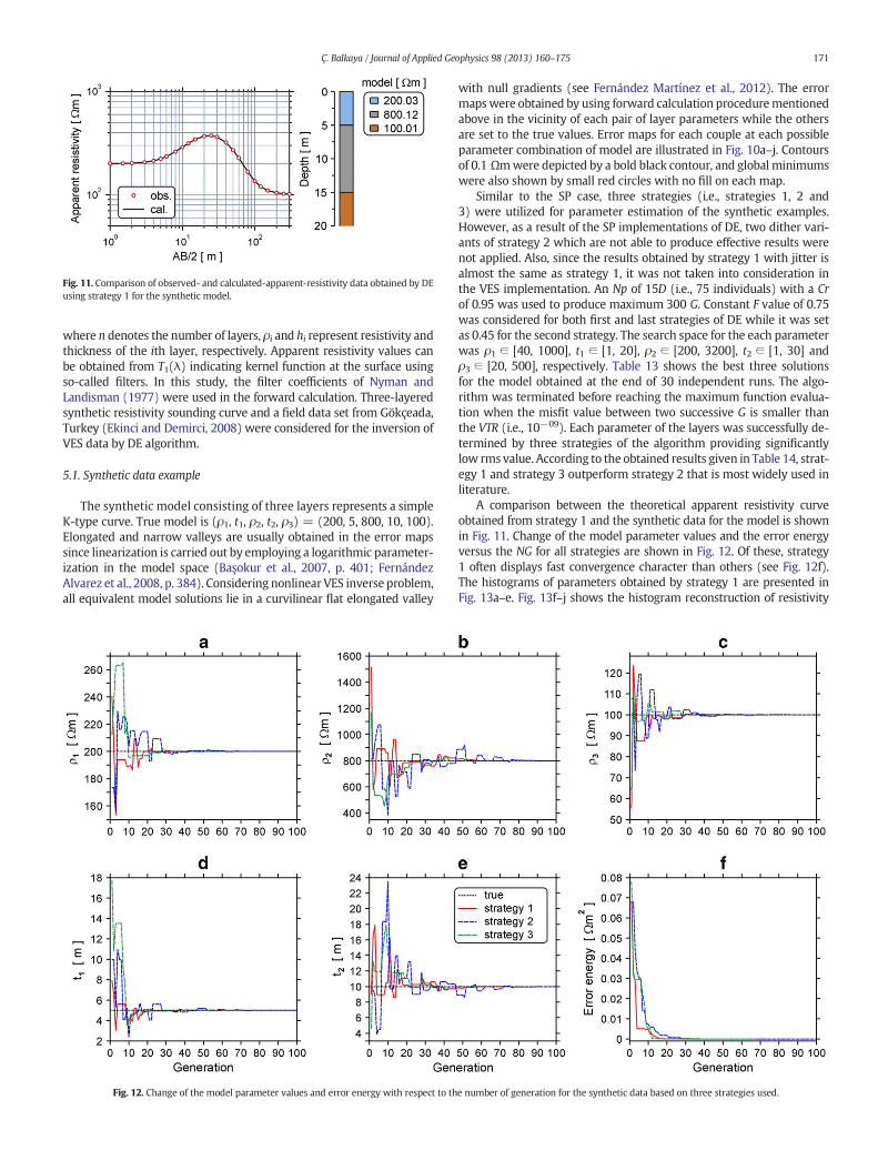
Fig. 11. Comparison of observed- and calculated-apparent-resistivity data obtained by DEusing strategy 1 for the synthetic model.

171Ç. Balkaya / Journal of Applied Geophysics 98 (2013) 160–175

where n denotes the number of layers, ρi and hi represent resistivity andthickness of the ith layer, respectively. Apparent resistivity values canbe obtained from T1(λ) indicating kernel function at the surface usingso-called filters. In this study, the filter coefficients of Nyman andLandisman (1977) were used in the forward calculation. Three-layeredsynthetic resistivity sounding curve and a field data set from Gökçeada,Turkey (Ekinci and Demirci, 2008) were considered for the inversion ofVES data by DE algorithm.

5.1. Synthetic data example

The synthetic model consisting of three layers represents a simpleK-type curve. True model is (ρ1, t1, ρ2, t2, ρ3) = (200, 5, 800, 10, 100).Elongated and narrow valleys are usually obtained in the error mapssince linearization is carried out by employing a logarithmic parameter-ization in the model space (Başokur et al., 2007, p. 401; FernándezAlvarez et al., 2008, p. 384). Considering nonlinear VES inverse problem,all equivalent model solutions lie in a curvilinear flat elongated valley

Fig. 12. Change of the model parameter values and error energy with respect to th

with null gradients (see Fernández Martínez et al., 2012). The errormapswere obtained by using forward calculation procedurementionedabove in the vicinity of each pair of layer parameters while the othersare set to the true values. Error maps for each couple at each possibleparameter combination of model are illustrated in Fig. 10a–j. Contoursof 0.1 Ωmwere depicted by a bold black contour, and global minimumswere also shown by small red circles with no fill on each map.

Similar to the SP case, three strategies (i.e., strategies 1, 2 and3) were utilized for parameter estimation of the synthetic examples.However, as a result of the SP implementations of DE, two dither vari-ants of strategy 2 which are not able to produce effective results werenot applied. Also, since the results obtained by strategy 1 with jitter isalmost the same as strategy 1, it was not taken into consideration inthe VES implementation. An Np of 15D (i.e., 75 individuals) with a Crof 0.95 was used to produce maximum 300 G. Constant F value of 0.75was considered for both first and last strategies of DE while it was setas 0.45 for the second strategy. The search space for the each parameterwas ρ1 ∈ [40, 1000], t1 ∈ [1, 20], ρ2 ∈ [200, 3200], t2 ∈ [1, 30] andρ3 ∈ [20, 500], respectively. Table 13 shows the best three solutionsfor the model obtained at the end of 30 independent runs. The algo-rithm was terminated before reaching the maximum function evalua-tion when the misfit value between two successive G is smaller thanthe VTR (i.e., 10−09). Each parameter of the layers was successfully de-termined by three strategies of the algorithm providing significantlylow rms value. According to the obtained results given in Table 14, strat-egy 1 and strategy 3 outperform strategy 2 that is most widely used inliterature.

A comparison between the theoretical apparent resistivity curveobtained from strategy 1 and the synthetic data for the model is shownin Fig. 11. Change of the model parameter values and the error energyversus the NG for all strategies are shown in Fig. 12. Of these, strategy1 often displays fast convergence character than others (see Fig. 12f).The histograms of parameters obtained by strategy 1 are presented inFig. 13a–e. Fig. 13f–j shows the histogram reconstruction of resistivity

e number of generation for the synthetic data based on three strategies used.

Fig. 13. (a–e) Frequencydistributions of eachparameter of syntheticmodel. (f–j)Histogram reconstructions fromparameter samples usingM–Halgorithmbased on the synthetic data set.Estimated parameters by DE implementation via strategy 1 are also indicated in each histogram.

172 Ç. Balkaya / Journal of Applied Geophysics 98 (2013) 160–175

and thickness for layers of the synthetic data by theM–H sampling usingSA that provides a range of plausible values for each parameter. In thesampling, the solutions obtained by strategy 1 were used. Lower andupper bounds of the layers were also constrained by the initial searchspaces mentioned above. Estimated parameters by DE are within thesampling limits of M–H as can be clearly observed on the histograms.

5.1.1. Effects of Np and NG on solutionConsidering various Np and NG, the effects of them on the solutions

were also analyzed for the model. Five different values of Np consisting

Table 15The best solutions for synthetic data set obtained by four different values ofNp andG at theend of 10 independent runs.

Np NG Resistivity (Ωm) Thickness (m) rms(Ωm)

Solutiona

(s)ρ1 ρ2 ρ3 t1 t2

20 25 200.571 918.949 100.166 5.062 8.712 0.0097 19.5350 200.121 786.084 99.999 4.980 10.184 5.99e−004 38.2875 200.029 799.731 100.005 5.001 10.004 1.09e−004 57.69

100 200.026 799.760 100.009 5.001 10.004 1.08e−004 78.0825 25 199.802 748.624 99.039 4.982 10.733 0.0065 23.60

50 199.992 785.910 100.028 4.972 10.194 4.54e−004 47.5175 200.024 799.274 100.009 5.000 10.011 1.09e−004 75.18

100 200.025 799.749 100.009 5.001 10.004 1.08e−004 99.1440 25 202.376 1041.651 100.202 5.383 7.468 0.0064 40.18

50 199.970 797.539 100.011 4.996 10.037 2.15e−004 83.7275 200.025 799.393 100.008 5.000 10.009 1.08e−004 121.16

100 200.026 799.766 100.009 5.001 10.004 1.08e−004 161.1850 25 198.893 700.463 100.420 4.712 11.647 0.0057 50.30

50 199.997 794.884 99.988 4.986 10.077 3.31e−004 97.3975 200.026 799.620 100.010 5.000 10.006 1.08e−004 147.09

100 200.026 799.745 100.009 5.001 10.004 1.08e−004 194.7875 25 200.986 1105.683 101.034 5.404 6.972 0.0057 74.36

50 200.050 792.914 100.000 4.986 10.100 2.85e−004 149.1175 200.025 799.951 100.013 5.001 10.001 1.09e−004 220.70

100 200.026 799.758 100.009 5.001 10.004 1.08e−004 324.78

a Average CPU time for each independent run.

of 20, 25, 40, 50, 75 and four different values of G for each Np were set,and strategy 1with a Cr of 0.95was used in the tests. The best results arelisted in Table 15. It is obvious that among the parameters, the resistiv-ities of first and last layers have the highest accuracy for each setting.Except the solutions obtained by the smallest NG (i.e., 25), each settingof Np with different values of G mentioned above has successfullyyielded true values of parameters. Considering all solutions (not fullydisplayed in Table 15) obtained at the end of the 10th independentrun for each different setting of Np and NG, relatively small Np (i.e., 20and 25) with 75 G in the algorithm yielded successful results withhigh success rates for the parameters than the other settings of G,especially for the resistivity and thickness of the second layer. Whenthe Np is relatively large (i.e., Np ≥ 40), more effective results wereobtained at the end of 75 and 100 G, respectively. The same rms values(i.e., 1.08e–004 Ωm) are obtained by the algorithmwith these settings.However, considering the average CPU times of the so-called solutionsgiven in Table 15, for instance in the case with 75 individuals keptfixed with 75 G yielded a time gain approximately 105 s per run com-pared to the same case with 100 G. Thus, it can be concluded that theeffective size of G is 75 for both relatively small and large populationsin the tests. A population size ranging from 8D to 15D is also proposedfor the initial choice of Np to invert VES data by DE. CPU times were

Table 16The best three solutions by DE at the end of 10 independent runs for the Gökçeada data.Best-fitting model parameters appear in boldface type.

Strategy Run Resistivity (Ωm) Thickness (m) rms(Ωm)

ρ1 ρ2 ρ3 ρ4 t1 t2 t3

1 1 47.730 17.460 1.165 353.463 2.601 11.489 4.500 0.03262 47.751 17.459 1.812 351.374 2.599 11.366 7.023 0.03265 47.795 17.456 1.617 350.112 2.597 11.396 6.261 0.0326

3 2 47.813 17.442 1.990 381.735 2.597 11.350 7.743 0.03269 47.844 17.472 1.988 345.836 2.593 11.300 7.702 0.0326

10 47.789 17.449 1.716 373.206 2.596 11.409 6.671 0.0326

Fig. 14. Comparison of observed- and calculated-apparent-resistivity data obtained by DEusing strategy 1 for the field data set.

173Ç. Balkaya / Journal of Applied Geophysics 98 (2013) 160–175

obtained with 3.07 GHz IBM PC compatible microcomputer with amemory of 8 GB.

5.2. Field data example

The DE algorithm was also used to interpret a field data set fromGökçeada (Turkey) characterized by a geological setting consisting ofa thick sedimentary sequence, volcanic rock and alluvium (Ekinci andDemirci, 2008). The study area is characterized by sandstone–shale se-quence overlying a resistive basal. The area is saturated with waterand also affected by seawater leakage. Relatively large initial searchspaces were used for estimating layer parameters; ρ1 and ρ2 ∈ [1,300], t1 ∈ [1, 20], ρ3 ∈ [1, 100], t2 and t3 ∈ [1, 30] and ρ4 ∈ [30,1500], respectively. The data were evaluated by the strategies 1 and 3considering the results obtained from the synthetic case. A populationof 105 individuals, that is Np of 15D, was used during the inversionbased on the results mentioned previously. Each run is terminatedwhen the maximum NG (i.e., 100) is reached. As seen in Table 16, the

Fig. 15. Histogram reconstructions by M–H algorithm based on the field data set. Estimated

solutions obtained by these two strategies are close to each other. Thefit between measured and calculated apparent resistivity data are illus-trated in Fig. 14. The top layer with the resistivity of 47.8 Ωm corre-sponds to consolidated alluvium. The second and third layers with thelower resistivities of 17.46 and 1.62 Ωm are related with the water sat-urated zone and the existence of seawater input in the medium. A rela-tively resistive geoelectrical basement at a depth of about 21 m has aresistivity of 350.11 Ωm. When comparing these results with thoseobtained by applying the M–H importance sampler (see Fig. 15a–g), itcan be concluded that DE is successful in determining seawater infiltra-tion into the freshwater zone between consolidated overburden layerconsisting of alluvium and relatively resistive basal.

6. Conclusions

DE algorithm was implemented to estimate parameters from theanomalies of SP and VES. Three mutation strategies commonly usedby DE were also extensively tested on both synthetic and field datasets. The results obtained from synthetic tests show that the algorithmprovided parameters very close to the true ones by avoiding gettingtrapped in local optima. The solutions obtained by DE for field datasets of SP are also in good agreement with PSO which is far the morewidely used than DE in the geophysical inverse problems. Among thestrategies used in all cases, the results obtained showed that strategy1 yields the better results with a good accuracy and less computationalcost. Strategy 3 also provided competitive results. Of the strategies,strategy 2 that appears to be the most successful and most widelyused generally demonstrates slow convergence characteristic and rela-tively high computational time requirement. In addition, its dithervariants display the worst performing for the inversion of SP data.Uncertainty in the solutions obtained by DE was also investigated byemploying SA without cooling based on the M–H algorithm. Accordingto the histogram reconstructions obtained, DE similar to other globaloptimization algorithms (i.e., PSO, GA) well estimated the model

parameters by DE implementation via strategy 1 are also indicated in each histogram.

174 Ç. Balkaya / Journal of Applied Geophysics 98 (2013) 160–175

parameters by providing higher posterior probabilities in the efficientM–H sampling in low-dimensional inverse geophysical problems.Even though previous studies on DE in other fields report successfullyresults, it has not been widely used in geophysics. Thus, it can be con-cluded that DEdeservesmore attention for the optimization of geophys-ical data.

Acknowledgments

I owe special thanks to Dr. Gökhan Göktürkler from Dokuz EylülUniversity, Izmir (Turkey) for his constructive and helpful comments,which greatly improved the paper. I would also like to thank the anon-ymous reviewers for their constructive comments that greatly contrib-uted to the improvement of the paper. I thank Yunus Levent Ekincifrom Çanakkale Onsekiz Mart University (Turkey) for providing thefield data set for VES. DE code was implemented using Scilab, the freesoftware for numerical computation (http://www.scilab.org/), whichis a trademark of INRIA (http://www.inria.fr/). Scilab version of DEalgorithm written by Walter Di Carlo and Helmut Jarausch is publiclyavailable online at http://www.icsi.berkeley.edu/~storn/code.html. APSO implementation developed by Sébastien Salmon for Scilab wasused in the test studies (http://atoms.scilab.org/toolboxes/PSO).

References

Abdelazeem, M., Gobashy, M., 2006. Self-potential inversion using genetic algorithm.JKAU Earth Sci. 17, 83–101.

Abdelrahman, E.M., Soliman, K.S., Abo-Ezz, E.R., Essa, K.S., El-Araby, T.M., 2009. Quantita-tive interpretation of self-potential anomalies of some simple geometric bodies. PureAppl. Geophys. 166, 2021–2035.

Balkaya, Ç., Göktürkler, G., 2012. Evaluation of four different stochastic approaches for esti-mating model parameters of self-potential. 4th Geoelectric Workshop, Çeşme (İzmir),pp. 53–57 (available at http://web.deu.edu.tr/yerelektrik2012/4.YEC_genisletilmis_bildiri_ozleri.pdf).

Balkaya, Ç., Göktürkler, G., Erhan, Z., Ekinci, Y.L., 2012. Exploration for a cave by magneticand electrical resistivity surveys: Ayvacık Sinkhole example, Bozdağ, İzmir (westernTurkey). Geophysics 77, B135–B146.

Başokur, A.T., Akça, I., Siyam, N.W.A., 2007. Hybrid genetic algorithms in view of theevolution theories with application for the electrical sounding method. Geophys.Prospect. 55, 393–406.

Bhattacharya, B.B., Roy, N., 1981. A note on the use of a nomogram for self-potentialanomalies. Geophys. Prospect. 29, 102–107.

Bogoslovsky, V.A., Ogilvy, A.A., 1977. Geophysical methods for the investigation of land-slides. Geophysics 42, 562–571.

Bolève, A., Janod, F., Revil, A., Lafon, A., Fry, J.-J., 2011. Localization and quantification ofleakages in dams using time-lapse self-potential measurements associated with salttracer injection. J. Hydrol. 403, 242–252.

Brest, J., Greiner, S., Bošković, B., Mernik, M., Žumer, V., 2006. Self-adapting control param-eters in differential evolution: a comparative study on numerical benchmark prob-lems. IEEE Trans. Evol. Comput. 10, 646–657.

Carlisle, A., Dozier, G., 2001. An off-the-shelf PSO. Proc. of the Workshop on ParticleSwarm Optimisation (Indianapolis: IN), pp. 1–6.

Chib, S., Greenberg, E., 1995. Understanding the Metropolis–Hastings algorithm. Am. Stat.49, 327–335.

Chunduru, R.K., Sen, M.K., Stoffa, P.L., 1997. Hybrid optimization methods for geophysicalinversion. Geophysics 62, 1196–1207.

Das, S., Konar, A., Chakraborty, U.K., 2005. Two improved differential evolutionschemes for faster global search. Proc. of the Genetic Evolution Computing Con-ference (Washington: USA), pp. 991–998.

Dittmer, J.K., Szymanski, J.E., 1995. The stochastic inversion of magnetics and resistivitydata using the simulated annealing algorithm. Geophys. Prospect. 43, 397–416.

Drahor, M.G., 2004. Application of the self-potential method to archaeological prospection:some case histories. Archaeol. Prospect. 11, 77–105.

Drahor, M.G., Berge, M.A., 2006. Geophysical investigation of the Seferihisar geothermalarea, Western Anatolia, Turkey. Geothermics 35, 302–320.

Ekinci, Y.L., Demirci, A., 2008. A damped least-squares inversion program for the interpre-tation of Schlumberger sounding curves. J. Appl. Sci. 8, 4070–4078.

El-Qady, G., Sakamoto, C., Ushijima, K., 1999. 2-D inversion of VES data in Saqqara archae-ological area, Egypt. Earth Planets Space 51, 1091–1098.

Fernández Alvarez, J.P., Fernández Martínez, J.L., Menéndez Pérez, C.O., 2008. Feasibilityanalysis of the use of binary genetic algorithms as importance samplers applicationto a geoelectrical VES inverse problem. Math. Geosci. 40, 375–408.

Fernández Martinez, J.L., Garcia Gonzalo, E., Fernández Álvarez, J.P., Kuzma, H.A.,Menéndez Pérez, C.O., 2010a. PSO: a powerful algorithm to solve geophysical inverseproblems: application to a 1D-DC resistivity case. J. Appl. Geophys. 71, 13–25.

Fernández-Martínez, J.L., García-Gonzalo, E., Naudet, V., 2010b. Particle swarm optimiza-tion applied to the solving and appraisal of the streaming potential inverse problem.Geophysics 75, WA3–WA15.

FernándezMartínez, J.L., Fernández-Muñiz, M.Z., Tompkins, M.J., 2012. On the topographyof the cost functional in linear and nonlinear inverse problems. Geophysics 77,W1–W15.

Gämperle, R.,Müller, S.D., Koumoutsakos, P., 2002. A parameter study for differential evolu-tion. In: Grmela, A., Mastorakis, N.E. (Eds.), Advances in Intelligent Systems, Fuzzy Sys-tems, Evolutionary Computation. WSEAS Press, Interlaken, Switzerland, pp. 293–298.

Ghosh, D.P., 1971a. The application of linear filter theory to the direct interpretation ofgeoelectrical resistivity sounding measurements. Geophys. Prospect. 19, 192–217.

Ghosh, D.P., 1971b. Inverse filter coefficients for the computation of apparent resistivitystandard curves for a horizontally strafied earth. Geophys. Prospect. 19, 769–775.

Göktürkler, G., 2011. A hybrid approach for tomographic inversion of crosshole seismicfirst-arrival times. J. Geophys. Eng. 8, 99–108.

Göktürkler, G., Balkaya, Ç., 2012. Inversion of self-potential anomalies caused by simple-geometry bodies using global optimization algorithms. J. Geophys. Eng. 9, 498–507.

Göktürkler, G., Balkaya, Ç., Erhan, Z., Yurdakul, A., 2008. Investigation of a shallow alluvialaquifer using geoelectricalmethods: a case fromTurkey. Environ. Geol. 54, 1283–1290.

Goswami, J.C., Mydur, R., Wu, P., Heliot, D., 2004. A robust technique for well-log datainversion. IEEE Trans. Antennas Propag. 52, 717–724.

Hamzah, U., Samsudin, A.R., Malim, A.P., 2007. Groundwater investigation in KualaSelangor using vertical electrical sounding (VES) surveys. Environ. Geol. 51,1349–1359.

Hastings, W., 1970. Monte Carlo sampling methods using Markov chains and their appli-cations. Biometrika 57, 97–109.

Heiland, C.A., Tripp, R.M., Dart, Wantland, 1945. Geophysical surveys at the MalachiteMine, Jefferson County, Colorado. Am. Inst. Min. Metall. Eng. 164, 142–154.

Holland, J.H., 1975. Adaptation in Natural and Artificial Systems: An Introductory Analysiswith Applications to Biology, Control, and Artificial Intelligence. University of Michi-gan Press, Ann Arbor, MI.

Huff, L.C., 1963. Comparison of geological, geophysical, and geochemical prospectingmethods at the Malachite mine, Jefferson County, Colorado: U.S. Geological Survey,Bulletin 1098-C, scale 1:2400.

Jha, M.K., Kumar, S., Chowdhury, A., 2008. Vertical electrical sounding survey and re-sistivity inversion using genetic algorithm optimization technique. J. Hydrol. 359,71–87.

Kennedy, J., Eberhart, R., 1995. Particle swarm optimisation. Proc. of IEEE InternationalConference on Neural Networks, Piscataway, New Jersey, pp. 1942–1948.

Kirkpatrick, S., Gelatt Jr., C.D., Vecchi, M.P., 1983. Optimisation by simulated annealing.Science 220, 671–680.

Koefoed, O., 1970. A fast method for determining the layer distribution from the raisedkernel function in geoelectrical soundings. Geophys. Prospect. 18, 564–570.

Koefoed, O., 1979. Geosounding Principles. Elsevier, Amsterdam.Li, X., Yin, M., 2012. Application of differential evolution algorithm on self-potential data.

PLoS One 7 (12), 1–11 (e51199).Lin, C., Qing, A., Feng, Q., 2011. A comparative study of crossover in differential evolution.

J. Heuristics 17, 675–703.Luo, X., 2010. Constraining the shape of a gravity anomalous body using reversible jump

Markov chain Monte Carlo. Geophys. J. Int. 180, 1067–1079.Mandal, A., Das, A.K., Mukherjee, P., Das, S., Suganthan, P.N., 2011. Modified differential

evolution with local search algorithm for real world optimization. Proc. of the IEEECongress on Evolutionary Computation, New Orleans, LA, USA, pp. 1565–1572.

Meiser, P., 1962. A method for quantitative interpretation of self potential measurements.Geophys. Prospect. 10, 203–218.

Metropolis, N., Rosenbluth, A.W., Rosenbluth, M.N., Teller, A.H., Teller, E., 1953. Equationsof state calculations by fast computing machines. J. Chem. Phys. 21, 1087–1091.

Mezura-Montes, E., Palomeque-Ortiz, A.G., 2009. Parameter control in differential evolu-tion for constrained optimization. Proc. of the IEEE Congress on Evolutionary Compu-tation, Trondheim, Norway, pp. 1375–1382.

Monteiro Santos, F.A., 2010. Inversion of self-potential of idealised bodies' anomaliesusing particle swarm optimisation. Comput. Geosci. 36, 1185–1190.

Mosegaard, K., Tarantola, A., 1995. Monte Carlo sampling of solutions to inverse problems.J. Geophys. Res. 100, 12431–12447.

Noman, N., Bollegala, D., Iba, H., 2011. An adaptive differential evolution algorithm.Proc. of the IEEE Congress on Evolutionary Computation, New Orleans, LA, USA,pp. 2229–2236.

Nyman, D.C., Landisman, M., 1977. VES dipole–dipole filter coefficients. Geophysics 42,1037–1044.

Özurlan, G., Candansayar, M.E., Şahin, M.H., 2006. Deep resistivity structure of the Dikili-Bergama region, west Anatolia, revealed by two-dimensional inversion of verticalelectrical sounding data. Geophys. Prospect. 54, 187–197.

Park, Y.H., Doh, S.J., Yun, S.T., 2007. Geoelectric resistivity sounding of riverside alluvialaquifer in an agricultural area at Buyeo, Geum River watershed, Korea: an applicationto groundwater contamination study. Environ. Geol. 53, 849–859.

Pekeris, C.L., 1940. Direct method of interpretation in resistivity prospecting. Geophysics5, 31–42.

Pekşen, E., Yas, T., Kayman, A.Y., Özkan, C., 2011. Application of particle swarm optimiza-tion on self-potential data. J. Appl. Geophys. 75, 305–318.

Price, K.V., Storn, R.M., Lampinen, J.A., 2005. Differential Evolution: A Practical Approachto Global Optimization. Springer-Verlag, Berlin.

Qing, A., 2009. Differential Evolution: Fundamentals and Applications in ElectricalEngineering. John Wiley & Sons, New York.

Reddi, A.G.B., Madhusudan, I.C., Sarkar, B., Sharma, J.K., 1982. An album of geophysicalresponses from base metal belts of Rajasthan and Gujarat. Geological Survey ofIndia Miscellaneous, Pub. No. 51.

Rönkkönen, J., Kukkonen, S., Price, K., 2005. Real-parameter optimization with differentialevolution. Proc. of the IEEE Congress on Evolutionary Computation, Edinburgh, UK,pp. 506–513.

175Ç. Balkaya / Journal of Applied Geophysics 98 (2013) 160–175

Růžek, B., Kvasnička, M., 2001. Diferential evolution algorithm in the earthquake hypo-center location. Pure Appl. Geophys. 158, 667–693.

Saraswat, P., Srivastava, R.P., Sen, M.K., 2010. Particle swarm and differential evolution —

optimization for stochastic inversion of post-stack seismic data. 8th Biennial Interna-tional Conference & Exposition on Petroleum Geophysics, Hyderabad, India.

Sen, M.K., Stoffa, P.L., 1995. Global Optimization Methods in Geophysical Inversion.Elsevier Science, The Netherlands.

Sen, M.K., Bhattachaya, B.B., Stoffa, P.L., 1993. Nonlinear inversion of resistivity soundingdata. Geophysics 58, 496–507.

Shaw, R., Srivastava, S., 2007. Particle swarm optimization: a new tool to invert geophys-ical data. Geophysics 72, F75–F83.

Srivastava, S., Agarwal, B.N.P., 2009. Interpretation of self-potential anomalies by en-hanced local wave number technique. J. Appl. Geophys. 68, 259–268.

Storn, R., 2008. Differential evolution research — trends and open questions. In:Chakraborty, U.K. (Ed.), Advances in Differential Evolution, SCI 143. Springer-Verlag,Berlin, pp. 1–31.

Storn, R., Price, K.V., 1995. Differential evolution— a simple and efficient adaptive schemefor global optimization over continuous spaces. Technical Report TR-95-012.Interna-tional Computer Science Institute, Berkeley.

Storn, R., Price, K., 1997. Differential evolution— a simple and efficient heuristic for globaloptimization over continuous spaces. J. Glob. Optim. 11, 341–359.

Tlas, M., Asfahani, J., 2008. Using of the adaptive simulated annealing (ASA) for quantita-tive interpretation of self-potential anomalies due to simple geometrical structures.JKAU Earth Sci. 19, 99–118.

Vichabian, Y., Morgan, F.D., 2002. Self potentials in cave detection. Lead. Edge 21,866–871.

Yüngül, S., 1950. Interpretation of spontaneous polarisation anomalies caused by spheroi-dal orebodies. Geophysics 15, 237–246.

Yüngül, S., 1954. Spontaneous potential survey of a copper deposit at Sarıyer, Turkey.Geophysics 19, 455–458.

Zaharie, D., 2009. Influence of crossover on the behavior of differential evolution algo-rithms. Appl. Soft Comput. 9, 1126–1138.