1 of 33

An Improved Corrections Process for Constrained Trajectory Design in the n-Body Problem

Belinda G. Marchand∗ and Kathleen C. Howell† Purdue University, West Lafayette, Indiana 47907-1282

Roby S. Wilson‡

Jet Propulsion Laboratory, Pasadena, California 91109

The general objective of this work is the development of efficient techniques for preliminary design of trajectories that must satisfy specific requirements such as periodicity, interior or boundary constraints, and coverage. Though the examples presented pertain to spacecraft mission design, the methodology developed is generally applicable to autonomous systems subject to algebraic constraints. For spacecraft mission design applications, an immediate advantage of this approach, particularly for the identification of periodic orbits, is that the startup solution need not exhibit any symmetry for the methodology to achieve the formulated objectives.

Nomenclature

t = time T = superscript denotes transpose operation k = subscript indicates the quantity is associated with the thk patch state * = superscript indicates the quantity is evaluated along the reference solution

, ,x y z = spacecraft position elements associated with current working reference frame , ,x y z = spacecraft velocity elements associated with the current working reference frame ( ) [ ], , TR t x y z= = column vector that denotes spacecraft position ( ) [ ], , TV t x y z= = column vector that denotes spacecraft velocity ( ) [ ], , Ta t x y z= = column vector that denotes the spacecraft acceleration ( ) ( ) ( ),

TX t R t V t⎡ ⎤= ⎣ ⎦ = column vector that denotes the spacecraft state

( )f X = a nonlinear vector function that depends explicitly on the spacecraft state δ = prefix denotes a variation measured relative to a reference arc

( )A t = Jacobian matrix ( )1,k kt t −Φ = 6 6× State Transition Matrix from an initial time, 1kt − , to a terminal time kt

, 1 , 1 , 1 , 1, , ,k k k k k k k kA B C D− − − − = 3 3× submatrices of ( )1,k kt t −Φ N = number of patch states along a startup solution

kVΔ = velocity discontinuity at the thk patch state

kα = vector of constraints at the thk patch state

kjα = the thj element of kα

∗ Visiting Assistant Professor, School of Aeronautics and /Astronautics, Purdue University; currently, Assistant Professor, Aerospace Engineering and Engineering Mechanics Department, University of Texas at Austin † Hsu Lo Professor of Aeronautical and Astronautical Engineering, School of Aeronautics and Astronautics, Purdue University ‡ Member of the Technical Staff, Jet Propulsion Laboratory

2 of 33

I. Introduction

From a dynamical perspective, the libration points have been the focus of many investigations since the initial

work of Poincaré [1]. In the last 20 years, periodic orbits in the three-body regime have successfully served as the

basis for trajectory design in various missions [2-8], from ISEE-3 [2-3] to the more recent Genesis mission [8]. As

the spacecraft applications of multi-body orbital analysis continue to expand, the goals and requirements are also

becoming ever more challenging. Thus, strategies to isolate preliminary trajectory arcs that satisfy a set of

constraints in this regime must be available.

Most optimization schemes, or other analysis tools in the full model, require a good startup solution. Thus, the

goal of this study is the development of a strategy to more efficiently produce preliminary designs for trajectories, in

multi-body regimes, when constraints are incorporated. Though the examples presented are related to spacecraft

mission design in the n-body problem, the generality of the method is preserved to accommodate other applications.

Ultimately, this approach represents a feasible numerical scheme for the determination of trajectory arcs in nonlinear

autonomous dynamical systems where the desired solution is subject to algebraic interior and/or exterior constraints.

The approach proposed here involves a sequence of increasingly complex steps [9-10]. Initially, the trajectory is

modeled as a series of arcs. The arcs may be determined from a three-body model, a multi-body numerical solution,

or a conic. An arc can also incorporate some additional force, if that is appropriate, such as solar radiation pressure.

This initial analysis is useful in establishing the general trajectory characteristics such as size, orientation, excursions

in the in-plane and out-of-plane directions, proximity to specified regions of space (perhaps the libration points), and

timing requirements. In the next step in the process, the specific constraints are modeled, as well as the associated

partials, if not already available. Then, a differential corrections process is employed to ensure position and velocity

continuity along the path while satisfying the constraints. The process can also be used to determine preliminary

requirements for maneuvers that may be necessary to satisfy the constraints. In the final step, the trajectory solution

is transitioned to a full model that incorporates any desired gravitational bodies, with ephemerides used for the

planetary locations.

3 of 33

It may include other forces – such as solar radiation pressure – as modeled previously. The focus of this effort, then,

is the further development of the mathematical relations and partials that are necessary to successfully merge the

arcs in the three-body environment such that the constraints are satisfied.

II. Background

In generating a preliminary solution, the capacity to develop a trajectory arc in the three- or four-body problem,

one that satisfies a set of constraints, is considered critical for an expanded design tool. For instance, a halo orbit

[11] is periodic and symmetric across a fundamental plane in the rotating frame of the restricted problem. Symmetry

and periodicity are both, in this case, constrained. However, an orbit can be periodic without being symmetric [12],

as is often the case in relative spacecraft motions [13] (i.e., formation flight) near the libration points.

In the restricted three-body problem, where the equations of motion are traditionally formulated in a synodic

coordinate system, a typical approach to determine a periodic path is to exploit the symmetry of the mathematical

model. First, a startup arc, such as that obtained from the Richardson approximation [14-15], is necessary. Once the

startup solution is available, the symmetry properties of the model, and the solution of interest, are employed in the

design of the differential corrector [11]. However, a differential corrector specifically developed around some

geometrical features will naturally only be applicable to trajectories that share those features. A traditional halo

corrector, for example, is only useful when searching for trajectories that are simply symmetric about the x-z plane.

As detailed in this investigation, it is possible to specify periodicity as a constraint, without prior knowledge of the

symmetry of the solution. This is particularly useful in exploring periodic orbits near the triangular points, or

establishing periodic formations near the libration points. In general, trajectory arcs of any kind can be subject to a

wide variety of point constraints during the mission design process. The development presented here is generalized

and applicable to any type of point constraint. It is assumed, of course, that the initial guess is still in the vicinity of

the desired solution.

4 of 33

Dynamical Model

Let X denote the spacecraft state such that [ ], , , , , TX x y z x y z= , where [ ], , Tx y z represent the spatial

coordinates of the vehicle and [ ], , Tx y z represent components of the spacecraft velocity associated with a generic

reference frame. Based on this definition, the nonlinear differential equations that govern the evolution of ( )X t , in

any gravitational regime, may be generally represented as,

( ) ( )( )X t f X t= , (1)

where the variable t represents time. Let 0t denote a reference time such that ( )0 0X t X= and ( )0 0X t X= identify

the reference state, and the associated time derivative, respectively. Then, according to Eq. (1), ( )0 0 0,X f X t= .

Note that both 0t and 0X can serve as a reference; that is, relative to this time and state, subsequent spacecraft states

may be expressed as a function of 0t , 0X , and perturbations relative to the reference, 0tδ and 0Xδ as follows,

0t t tδ= + , (2) ( ) ( )0 0X t X t Xδ= + . (3)

The variational equation associated with Eq. (1) is of the form,

( )X A t Xδ δ= , (4) where

( )0 0,X t

fA tX

∂=∂

, (5)

represents the Jacobian matrix evaluated along the reference solution. The solution to this variational equation is

well known and depends on the state transition matrix (STM), 1 0( , )t tΦ ,

( ) ( ) ( )1 1 0 0,X t t t X tδ δ= Φ . (6)

The STM is determined by numerical integration of the matrix differential equation,

( ) ( ) ( )1 0 1 0, ,t t A t t tΦ = Φ , (7)

subject to the initial condition ( )0 0,t t IΦ = , and I denotes a properly dimensioned identity matrix. The variation in

Eq. (6) is said to be contemporaneous. That is, the variation ( )X tδ is the difference between the actual nonlinear

state, ( )X t , and the neighboring nominal state, ( )0X t , evaluated precisely at time t .

5 of 33

However, the derivation of a differential corrections process benefits from the introduction of a non-

contemporaneous variation,

( ) ( ) ( )X X t X t X t tδ δ δ δ′ ′= = + , (8)

where t t tδ ′= − . The relation between the contemporaneous and non-contemporaneous variation is illustrated

graphically in Fig. 1.

Fig. 1 — Contemporaneous versus Non-Contemporaneous Variations

Substitution of Eq. (8) into Eq. (6) yields the following expression,

( ) ( )( ) ( ) ( ) ( )( )1 1 1 1 1 0 0 0 0 0,X t t X t t t t X t t X t tδ δ δ δ δ δ′ ′+ − = Φ + − . (9)

If the initial time for the numerical propagation is held fixed, relative to the nominal initial time, then 0 0tδ = and

Eq. (9) can be further reduced, i.e.,

( )1 1 0 0 1 1,X t t X X tδ δ δ′ ′= Φ + . (10)

Eq. (10) is the basis of a standard two level differential corrector.

Level I Differential Corrector

A differential corrections process requires a startup solution. Such a trajectory arc may be the result of a

numerical integration process [16], perhaps one such that the path does not necessarily satisfy the specified

constraints. An initial guess can also be constructed from a series expansion [14-15] that approximates the solution.

Other alternatives, even conics, can also serve as a startup arc in the ephemeris model.

6 of 33

Once available, the startup solution is decomposed into segments and nodes or patch points. The goal of the Level I

corrector is simple, that is, to achieve position continuity — in the nonlinear model — across all trajectory segments.

The development of the Level I corrections process [17] is presented here for notational completeness.

Suppose a startup trajectory arc is decomposed into 1N − segments and N nodes. Each segment is

characterized by an initial time, 1kt − , and a terminal time, kt , where 1, ,k N= … . At the initial point along a

segment, the six-dimensional state vector is defined in terms of two three-element vectors, i.e.,

1 1 1

T

k k kX R V− − −⎡ ⎤= ⎣ ⎦ , while the terminal state vector is written T

k k kX R V⎡ ⎤= ⎣ ⎦ . The formulation for the Level I

corrector can summarized as follows,

fixed constraints :

1 1 10 ; 0k k k kR R t tδ δ δ δ− − −′ = = = = (11)targets : *

k k k kR R R Rδ δ′ = − = (12)controls :

1 1k kV Vδ δ− −′ = (13)free :

k kV Vδ δ′ = (14)

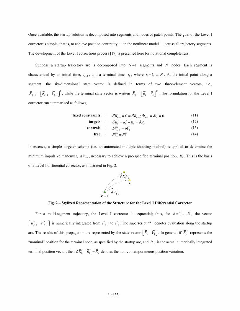
In essence, a simple targeter scheme (i.e. an automated multiple shooting method) is applied to determine the

minimum impulsive maneuver, 1kV −Δ , necessary to achieve a pre-specified terminal position, kR . This is the basis

of a Level I differential corrector, as illustrated in Fig. 2.

Fig. 2 – Stylized Representation of the Structure for the Level I Differential Corrector

For a multi-segment trajectory, the Level I corrector is sequential; thus, for 1, ,k N= … , the vector

* *1 1k kR V− −⎡ ⎤⎣ ⎦ is numerically integrated from *

1kt − to *kt . The superscript “*” denotes evaluation along the startup

arc. The results of this propagation are represented by the state vector k kR V⎡ ⎤⎣ ⎦ . In general, if *kR represents the

“nominal” position for the terminal node, as specified by the startup arc, and kR is the actual numerically integrated

terminal position vector, then *k k kR R Rδ ′ = − denotes the non-contemporaneous position variation.

7 of 33

Implementation of the assumptions in Eq. (11)-(14), to the illustration in Fig. 1, further implies that k kR Rδ δ′ = . The

control variable that drives the iterative process is *1 1 1k k kV V V− − −Δ = − , where *

1 1 1k k kV V Vδ− − −= + ; thus, 1 1k kV Vδ− −Δ = .

Consider Eq. (9) within the context of the notation in Fig. 2 where, as presently written, 1k = . In general, the

6 6× state transition matrix (STM), ( )1,k kt t −Φ , can be subdivided into four 3 3× submatrices such that

( ) , 1 , 11

, 1 , 1

, k k k kk k

k k k k

A Bt t

C D− −

−− −

⎡ ⎤Φ = ⎢ ⎥

⎣ ⎦. (15)

The subscript pair “ , 1k k − ” denotes the direction of the propagation. For example, the right subscript, “ 1k − ”,

denotes the start time ( 1kt − ) of the propagation, while the subscript to the left, “ k ”, reflects the terminal time kt .

Consequently, ( ) ( )11 1, ,k k k kt t t t−

− −Φ = Φ may also be decomposed into sub-matrices,

( ) 1, 1,1

1, 1,

, k k k kk k

k k k k

A Bt t

C D− −

−− −

⎡ ⎤Φ = ⎢ ⎥

⎣ ⎦. (16)

Employing this subscript notation in Eq. (9), the variational equations for the segment in Fig. 2 may be rewritten as,

, 1 , 1 1 1 1

, 1 , 11 1 1

k k k kk k k k k k

k k k kk k k k k k

A BR V t R V tC DV a t V a t

δ δ δ δ

δ δ δ δ− − − − −

− −− − −

⎡ ⎤ ⎡ ⎤′ ′− −⎡ ⎤⎢ ⎥ ⎢ ⎥= ⎢ ⎥⎢ ⎥ ⎢ ⎥′ ′⎣ ⎦− −⎣ ⎦ ⎣ ⎦

. (17)

In Eq. (17), kV and ka represent the actual nonlinear velocity and acceleration vectors, along the current

solution, as highlighted in Fig. 1, at the terminal node. Similarly, 1kV − and 1ka − are the velocity and acceleration

associated with the initial node on the current trajectory segment. The vector 1kRδ −′ is the difference, or non-

contemporaneous variation, in position between the initial node on the current solution and the initial node on the

nominal solution, as detailed in Fig. 1. The vector 1kVδ −′ denotes the non-contemporaneous variation in velocity

between the current and nominal solutions. Similar definitions apply for kRδ ′ and kVδ ′ .

Note that, in linear systems analysis, the submatrices , 1k kA − , , 1k kB − , , 1k kC − , and , 1k kD − are typically associated

with a pre-specified reference solution, one that is known as a function of time. In a differential corrections process,

however, the complete nominal trajectory is not necessarily known a priori. Instead, design constraints are imposed

and the goal is to identify an arc that best satisfies these constraints.

8 of 33

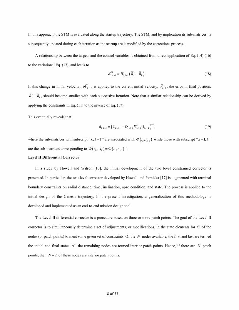
In this approach, the STM is evaluated along the startup trajectory. The STM, and by implication its sub-matrices, is

subsequently updated during each iteration as the startup arc is modified by the corrections process.

A relationship between the targets and the control variables is obtained from direct application of Eq. (14)-(16)

to the variational Eq. (17), and leads to

( )1 *1 , 1k k k k kV B R Rδ −

− −= − . (18)

If this change in initial velocity, 1kVδ − , is applied to the current initial velocity, 1kV − , the error in final position,

*k kR R− , should become smaller with each successive iteration. Note that a similar relationship can be derived by

applying the constraints in Eq. (11) to the inverse of Eq. (17).

This eventually reveals that

( ) 11, 1 1, 1, 1, 1,k k k k k k k k k kB C D B A

−−− − − − −= − , (19)

where the sub-matrices with subscript “ , 1k k − ” are associated with ( )1,k kt t −Φ while those with subscript “ 1,k k− ”

are the sub-matrices corresponding to ( ) ( ) 11 1, ,k k k kt t t t −

− −Φ = Φ .

Level II Differential Corrector

In a study by Howell and Wilson [10], the initial development of the two level constrained corrector is

presented. In particular, the two level corrector developed by Howell and Pernicka [17] is augmented with terminal

boundary constraints on radial distance, time, inclination, apse condition, and state. The process is applied to the

initial design of the Genesis trajectory. In the present investigation, a generalization of this methodology is

developed and implemented as an end-to-end mission design tool.

The Level II differential corrector is a procedure based on three or more patch points. The goal of the Level II

corrector is to simultaneously determine a set of adjustments, or modifications, in the state elements for all of the

nodes (or patch points) to meet some given set of constraints. Of the N nodes available, the first and last are termed

the initial and final states. All the remaining nodes are termed interior patch points. Hence, if there are N patch

points, then 2N − of these nodes are interior patch points.

9 of 33

An example problem with three patch points is represented in Fig. 3, where the subscript 1k − denotes the initial

state along one segment, 1k + identifies the final state on the next segment, and k is associated with the interior

state that connects the two consecutive segments. The state vector at the initiation of a numerical propagation

process is labeled with a superscript “+”, while that at the end of a propagation is labeled with the superscript “-”.

The goal of the Level I corrections process is to achieve position continuity across segments, k kR R+ −= . Once this

is achieved, the next level of the corrections process enforces any given number of constraints on any of the N

patch points available. For instance, Pernicka and Howell [17] employ a two level corrector to enforce velocity

continuity at each of the interior points. In this case, 3 scalar constraints are imposed on each interior point,

k kV V+ −= for 2, , 1k N= −… .

Fig. 3 – Stylized Representation of Level II Differential Corrector

Velocity continuity across segments is formulated [10,17] as a constraint, applied at the kth node, such that

* 0k k kV V V+ −− − Δ = , where *kVΔ represents the desired value of the impulsive maneuver at the kth node. Then, the

goal of a Level II corrections process is to minimize the constraint error. The control variables available to enforce

the constraints at the nodes are the positions and times associated with the nodes themselves. Thus, the patch points

in the Level II corrector are allowed to “float” in a sense.

10 of 33

The next step in a generalized Level II corrector is to establish a relationship between the control variables and

the constraint equations. To that end, consider the following set of variational equations associated with each of the

segments in Fig. 3, i.e.,

( )( )

( )( )

1 1 1, 1 , 1

, 1 , 11 1 1

k k k k k kk k k k

k k k kk k k k k k

R V t R V tA BC DV a t V a t

δ δ δ δ

δ δ δ δ

− +− − + +− − −− −

− +− − + +− −− − −

⎡ ⎤ ⎡ ⎤′ ′− −⎡ ⎤⎢ ⎥ ⎢ ⎥= ⎢ ⎥⎢ ⎥ ⎢ ⎥⎣ ⎦′ ′− −⎣ ⎦ ⎣ ⎦

, (20)

( )( )

( )( )

1 1 1, 1 . 1

, 1 , 11 1 1

k k k k k kk k k k

k k k kk k k k k k

R V t R V tA BC DV a t V a t

δ δ δ δ

δ δ δ δ

+ −+ + − −+ + ++ +

+ −+ + − −+ ++ + +

⎡ ⎤ ⎡ ⎤′ ′− −⎡ ⎤⎢ ⎥ ⎢ ⎥= ⎢ ⎥⎢ ⎥ ⎢ ⎥⎣ ⎦′ ′− −⎣ ⎦ ⎣ ⎦

. (21)

Note that, in Eq. (21), the flow of the second segment is reversed to evolve from 1kt + to kt . In the present

development, each trajectory segment is treated independently with respect to the rest of the segments along the

solution. For example, the variations in the initial state at 1kt+− do not directly affect changes on the second segment,

from kt+ to 1kt

−+ . This results directly from the sequential nature of the Level 1 corrector.

Using the same terminology employed previously, the formulation for this particular Level II differential corrector is

fixed constraints : 0; 0k k k kR R t t+ − + −− = − = (22)targets : ( ) * *

k k k k k kV V V V V Vδ δ+ − + −− − Δ = − − Δ (23)

controls : 1 1 1 1, , , , ,k k k k k kR t R t R tδ δ δ δ δ δ− − + + (24)

free : 1 1,k kV Vδ δ+ −

− + (25)

Note that, if a deterministic maneuver is allowed at the thk node, then * 0kVΔ ≠ . Based on Eq. (23), there are

( )2 3N − × targets, three for each interior patch point. The control variables, as previously stated, are the position

and times of all N patch points. Thus, in general, there are 4N × control parameters. Beyond the initial

investigation by Pernicka and Howell [17], it is also possible to specify arbitrary constraints at any of the N patch

points [10]. These constraints become additional targets in a Level II corrections process. In the following section,

additional constraints are presented to supplement those originally presented by Howell and Wilson [10] and expand

the generality of the method. Note that, unless too many constraints are specified, this system will naturally be

underdetermined.

11 of 33

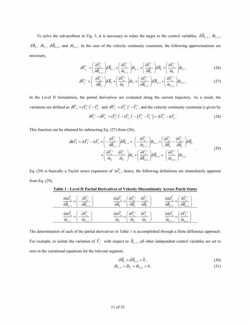
To solve the sub-problem in Fig. 3, it is necessary to relate the target to the control variables, 1kRδ − , 1ktδ − ,

kRδ , ktδ , 1kRδ + , and 1ktδ + . In the case of the velocity continuity constraint, the following approximations are

necessary,

1 11 1

k k k kk k k k k

k k k k

V V V VV R t R t

R t R tδ δ δ δ δ

− − − −−

− −− −

⎛ ⎞ ⎛ ⎞ ⎛ ⎞ ⎛ ⎞∂ ∂ ∂ ∂= + + +⎜ ⎟ ⎜ ⎟ ⎜ ⎟ ⎜ ⎟∂ ∂ ∂ ∂⎝ ⎠ ⎝ ⎠ ⎝ ⎠ ⎝ ⎠

, (26)

1 11 1

k k k kk k k k k

k k k k

V V V VV R t R t

R t R tδ δ δ δ δ

+ + + ++

+ ++ +

⎛ ⎞ ⎛ ⎞ ⎛ ⎞ ⎛ ⎞∂ ∂ ∂ ∂= + + +⎜ ⎟ ⎜ ⎟ ⎜ ⎟ ⎜ ⎟∂ ∂ ∂ ∂⎝ ⎠ ⎝ ⎠ ⎝ ⎠ ⎝ ⎠

. (27)

In the Level II formulation, the partial derivatives are evaluated along the current trajectory. As a result, the

variations are defined as *( )k k kV V Vδ − − −= − and *( )k k kV V Vδ + + += − , and the velocity continuity constraint is given by

( )* * *( ) ( )k k k k k k k kV V V V V V V Vδ δ+ − + − + −− = − − − = Δ − Δ . (28)

This function can be obtained by subtracting Eq. (27) from (26),

*1 1

1 1

1 11 1

k k k kk k k k k k

k k k k

k k k kk k k

k k k k

V V V VV V V R t R

R t R R

V V V Vt R t

t t R t

δ δ δ δ

δ δ δ

− − + −

− −− −

+ − + +

+ ++ +

⎛ ⎞ ⎛ ⎞ ⎛ ⎞∂ ∂ ∂ ∂Δ = Δ − Δ = − + − + −⎜ ⎟ ⎜ ⎟ ⎜ ⎟∂ ∂ ∂ ∂⎝ ⎠ ⎝ ⎠ ⎝ ⎠

⎛ ⎞ ⎛ ⎞ ⎛ ⎞∂ ∂ ∂ ∂+ − + +⎜ ⎟ ⎜ ⎟ ⎜ ⎟∂ ∂ ∂ ∂⎝ ⎠ ⎝ ⎠ ⎝ ⎠

. (29)

Eq. (29) is basically a Taylor series expansion of kVΔ ; hence, the following definitions are immediately apparent

from Eq. (29),

Table 1 - Level II Partial Derivatives of Velocity Discontinuity Across Patch States

1 1

k k

k k

V VR R

−

− −

⎛ ⎞∂Δ ∂= −⎜ ⎟∂ ∂⎝ ⎠

k k k

k k k

V V VR R R

+ −⎛ ⎞∂Δ ∂ ∂= −⎜ ⎟∂ ∂ ∂⎝ ⎠

1 1

k k

k k

V VR R

+

+ +

⎛ ⎞∂Δ ∂= ⎜ ⎟∂ ∂⎝ ⎠

1 1

k k

k k

V Vt t

−

− −

⎛ ⎞∂Δ ∂= −⎜ ⎟∂ ∂⎝ ⎠

k k k

k k k

V V Vt t t

+ −⎛ ⎞∂Δ ∂ ∂= −⎜ ⎟∂ ∂ ∂⎝ ⎠

1 1

k k

k k

V Vt t

+

+ +

⎛ ⎞∂Δ ∂= ⎜ ⎟∂ ∂⎝ ⎠

The determination of each of the partial derivatives in Table 1 is accomplished through a finite difference approach.

For example, to isolate the variation of kV − with respect to 1kR − , all other independent control variables are set to

zero in the variational equations for the relevant segment,

1 0k kR Rδ δ += = , (30) 1 1 0k k kt t tδ δ δ− += = = . (31)

12 of 33

As a result, the partial derivative can be approximated as 1 1/ /k k k kV R V Rδ δ− −− −∂ ∂ ≈ . The variations necessary to

construct these partials may be obtained through algebraic manipulation of the variational Eq. (20) or (21). The

results of this finite difference approximation are presented in Table 2.

Table 2 - Partial Derivatives of Velocity Relative To Patch State Control Variables

11,

1

kk k

k

VB

R

−−−

−

∂=

∂ 1

1, 1,k

k k k kk

VB A

R

−−− −

∂= −

∂ 1

1, 1,k

k k k kk

VB A

R

+−+ +

∂= −

∂ 1

1,1

kk k

k

VB

R

+−+

+

∂=

∂

11, 1

1

kk k k

k

VB V

t

−− +− −

−

∂= −

∂ ( )1

, 1 , 1k

k k k k k kk

Va D B V

t

−− − −

− −∂

= −∂

( )1, 1 , 1

kk k k k k k

k

Va D B V

t

++ − +

+ +∂

= −∂

11, 1

1

kk k k

k

VB V

t

+− −+ +

+

∂= −

∂

For the Level II velocity continuity constraint, substitution of the above partials into the expressions in Table 1

leads to the results in Table 3. The traditional statement [17] of the Level II corrector is

1

1

*

1 1 1 1

1

1

k

k

kk k k k k kk k k

k k k k k k k

k

k

b

RtRV V V V V V

V V VR t R t R t t

RMt

δδδ

δδ

δδ

−

−

− − + +

+

+

⎡ ⎤⎢ ⎥⎢ ⎥⎢ ⎥⎡ ⎤∂Δ ∂Δ ∂Δ ∂Δ ∂Δ ∂Δ

Δ = Δ − Δ = ⎢ ⎥⎢ ⎥∂ ∂ ∂ ∂ ∂ ∂ ⎢ ⎥⎣ ⎦⎢ ⎥⎢ ⎥⎢ ⎥⎣ ⎦

. (32)

In Eq. (32), the matrix M, containing all of the partial derivatives in Table 3, is termed the State Relationship Matrix

(SRM) and b denotes the vector of variations in position and time. The linear system in Eq. (32) can subsequently

be summarized as kV MbδΔ = .

Table 3 – Summary of Partial Derivatives for Level II: Velocity Constraints at Interior Patch Points

11,

1

kk k

k

VB

R−−

−

∂Δ= −

∂ 1 1

1, 1, 1, 1,k

k k k k k k k kk

VB A B A

R− −− − + +

∂Δ= −

∂ 1

1,1

kk k

k

VB

R−+

+

∂Δ=

∂

11, 1

1

kk k k

k

VB V

t− +− −

−

∂Δ=

∂

1 1, 1 , 1 , 1 , 1

kk k k k k k k k k k k k

k

Va a D B V D B V

t+ − − − − +

− − + +∂Δ

= − + −∂

or 1 11, 1, 1, 1,

kk k k k k k k k k k k k

k

Va a B A V B A V

t+ − − − − +

− − + +∂Δ

= − − +∂

11, 1

1

kk k k

k

VB V

t− −+ +

+

∂Δ= −

∂

In a well posed problem, the system is underdetermined; that is, there are more control variables than target

quantities. Hence, an infinite number of solutions exist. In a traditional corrections process, the minimum Euclidean

norm solution is selected. The minimum norm solution is well known and computed as,

( ) 1T Tkb M MM Vδ

−= Δ . (33)

13 of 33

The results from Eq. (33) suggest possible changes in the positions and times of each patch state that may minimize

the constraint equations. These changes are applied in the nonlinear system and the Level I iteration is repeated to

achieve position continuity. Of course, the changes suggested by Eq. (33) only lead to a minimum norm solution in

the linear system. In reality, it is unlikely that the modified nonlinear path will meet the constraints exactly after

position continuity is re-established in the nonlinear system. At best, the updated nonlinear path will more closely

follow the given constraints.

These changes are added to the patch point states and the trajectory is recomputed using a Level I differential

corrections process. If a solution exists, the interior kVΔ ’s should decrease, or approach the nominal value, with

every successive iteration.

Level II with Constraints

It is frequently necessary to specify additional constraints along a particular trajectory solution. The Level II

differential corrector described in the previous section can be modified to allow general constraints at any of the

patch points that describe the solution. This is possible as long as the constraint is of the form

( ), , ,kj kj k k k kR V V tα α + −= , (34)

or

( ), ,kj kj k k kR V tα α= . (35)

Thus, the scalar constraint kjα must be expressed as a function of the position, velocity, and time that correspond to

the patch point. The first subscript index, k, on the constraint denotes the patch point with which the constraint is

associated. The second index, j, denotes the constraint number at that patch point. This allows for multiple

constraints at multiple patch points. Let *kjα represent the desired value of this algebraic constraint. Also, recall that

the control variables in a Level II corrector are 1kRδ − , 1ktδ − , kRδ , ktδ , 1kRδ + , and 1ktδ + .

To incorporate these constraints into the corrections process, it is necessary to establish a relationship between

the targets, *kj kj kjδα α α= − , and the control variables. By definition, kjα can depend explicitly on kR and kt .

However, there is no explicit dependence on the remaining control variables. Instead, the constraint may also depend

on either kV + or kV − , or both.

14 of 33

This introduces an implicit dependence on the other control variables since the velocity discontinuities at the thk

patch point are related to the position and times of the nodes neighboring the patch point of interest; in particular,

( )1 1, , ,k k k k k kV V R t R t+ ++ += , (36)

( )1 1, , ,k k k k k kV V R t R t− −− −= . (37)

Thus, the constraint equation can also be approximated, to first order, through the following Taylor Series

expansion,

*1 1

1 1 1 1 1 1

kj kj kj kj kj kjk k k kkj kj k k

k k k k k kk k k k

kj kj kj kjk kk

k k k kk k

V V V VR t

R R R t t tV V V V

V VR

R R R tV V

α α α α α αα α δ δ

δ δα α α α

δδ δ δ

+ − + −

− −+ − + −− − − − − −

+ −

+ −

∂ ∂ ∂ ∂ ∂ ∂⎛ ⎞ ⎛ ⎞∂ ∂ ∂ ∂= + + + + + +⎜ ⎟ ⎜ ⎟∂ ∂ ∂ ∂∂ ∂ ∂ ∂⎝ ⎠ ⎝ ⎠

∂ ∂ ∂ ∂ ∂⎛ ⎞∂ ∂+ + + + +⎜ ⎟∂ ∂ ∂⎝ ⎠

1 11 1 1 1 1 1

kj kjk kk

k kk k

kj kj kj kj kj kjk k k kk k

k k k k k kk k k k

V Vt

t tV V

V V V VR t

R R R t t tV V V V

α αδ

α α α α α αδ δ

δ δ

+ −

+ −

+ − + −

+ ++ − + −+ + + + + +

∂⎛ ⎞∂ ∂+⎜ ⎟∂ ∂∂ ∂⎝ ⎠

∂ ∂ ∂ ∂ ∂ ∂⎛ ⎞ ⎛ ⎞∂ ∂ ∂ ∂+ + + + + +⎜ ⎟ ⎜ ⎟∂ ∂ ∂ ∂∂ ∂ ∂ ∂⎝ ⎠ ⎝ ⎠

. (38)

Note that the partial derivatives in Eq. (38) are evaluated along the current solution, kjα represents the current

value of the constraint at the kth node, and *kjα represents the desired value of the constraint. This expression may be

further simplified by applying the definitions in Eq. (34), (36), and (37), that is,

1 1

0kj kj

k kR Rα α

− +

∂ ∂= =

∂ ∂ , (39)

1 1

0kj kj

k kt tα α

− +

∂ ∂= =

∂ ∂ , (40)

1 1

0k k

k k

V VR R

+ −

− +

∂ ∂= =

∂ ∂ , (41)

1 1

0k k

k k

V Vt t

+ −

− +

∂ ∂= =

∂ ∂ . (42)

Substitution of Eq. (39)-(42) into Eq. (38) leads to the following variational constraint equation,

1 11 1

kj kjk kkj k k

k kk k

kj kj kj kj kjk kk

k k k kk k k

V VR t

R tV V

V VR

R R R tV V V

α αδα δ δ

α α α α αδ

δ δ δ

− −

− −− −− −

+ −

+ −

∂ ∂⎛ ⎞ ⎛ ⎞∂ ∂= +⎜ ⎟ ⎜ ⎟∂ ∂∂ ∂⎝ ⎠ ⎝ ⎠

∂ ∂ ∂ ∂ ∂⎛ ⎞∂ ∂+ + + + +⎜ ⎟∂ ∂ ∂ ∂⎝ ⎠

1 11 1

kjk kk

k kk

kj kjk kk k

k kk k

V Vt

t tV

V VR t

R tV V

αδ

α αδ δ

+ −

+ −

+ +

+ ++ ++ +

∂⎛ ⎞∂ ∂+⎜ ⎟∂ ∂∂⎝ ⎠

∂ ∂⎛ ⎞ ⎛ ⎞∂ ∂+ +⎜ ⎟ ⎜ ⎟∂ ∂∂ ∂⎝ ⎠ ⎝ ⎠

. (43)

15 of 33

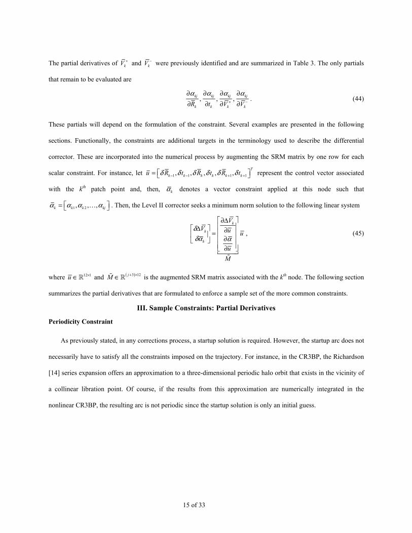
The partial derivatives of kV + and kV − were previously identified and are summarized in Table 3. The only partials

that remain to be evaluated are

, , ,kj kj kj kj

k k k kR t V Vα α α α

+ −

∂ ∂ ∂ ∂∂ ∂ ∂ ∂

. (44)

These partials will depend on the formulation of the constraint. Several examples are presented in the following

sections. Functionally, the constraints are additional targets in the terminology used to describe the differential

corrector. These are incorporated into the numerical process by augmenting the SRM matrix by one row for each

scalar constraint. For instance, let 1 1 1 1, , , , ,T

k k k k k ku R t R t R tδ δ δ δ δ δ− − + +⎡ ⎤= ⎣ ⎦ represent the control vector associated

with the kth patch point and, then, kα denotes a vector constraint applied at this node such that

1 2, ,k k k kjα α α α⎡ ⎤= ,⎣ ⎦… . Then, the Level II corrector seeks a minimum norm solution to the following linear system

k

k

k

VV u u

uM

δδα α

⎡ ⎤∂Δ⎢ ⎥⎡ ⎤Δ ∂⎢ ⎥=⎢ ⎥ ∂⎢ ⎥⎣ ⎦⎢ ⎥∂⎣ ⎦

, (45)

where 12 1u ×∈R and ( )3 12jM + ×∈R is the augmented SRM matrix associated with the kth node. The following section

summarizes the partial derivatives that are formulated to enforce a sample set of the more common constraints.

III. Sample Constraints: Partial Derivatives

Periodicity Constraint

As previously stated, in any corrections process, a startup solution is required. However, the startup arc does not

necessarily have to satisfy all the constraints imposed on the trajectory. For instance, in the CR3BP, the Richardson

[14] series expansion offers an approximation to a three-dimensional periodic halo orbit that exists in the vicinity of

a collinear libration point. Of course, if the results from this approximation are numerically integrated in the

nonlinear CR3BP, the resulting arc is not periodic since the startup solution is only an initial guess.

16 of 33

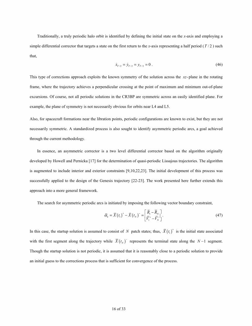
Traditionally, a truly periodic halo orbit is identified by defining the initial state on the x-axis and employing a

simple differential corrector that targets a state on the first return to the x-axis representing a half period ( / 2T ) such

that,

/ 2 / 2 / 2 0T T Tx y y= = = . (46)

This type of corrections approach exploits the known symmetry of the solution across the -xz plane in the rotating

frame, where the trajectory achieves a perpendicular crossing at the point of maximum and minimum out-of-plane

excursions. Of course, not all periodic solutions in the CR3BP are symmetric across an easily identified plane. For

example, the plane of symmetry is not necessarily obvious for orbits near L4 and L5.

Also, for spacecraft formations near the libration points, periodic configurations are known to exist, but they are not

necessarily symmetric. A standardized process is also sought to identify asymmetric periodic arcs, a goal achieved

through the current methodology.

In essence, an asymmetric corrector is a two level differential corrector based on the algorithm originally

developed by Howell and Pernicka [17] for the determination of quasi-periodic Lissajous trajectories. The algorithm

is augmented to include interior and exterior constraints [9,10,22,23]. The initial development of this process was

successfully applied to the design of the Genesis trajectory [22-23]. The work presented here further extends this

approach into a more general framework.

The search for asymmetric periodic arcs is initiated by imposing the following vector boundary constraint,

( ) ( ) 11

1

Nk N

N

R RX t X t

V Vα + −

+ −

⎡ ⎤−= − = ⎢ ⎥−⎣ ⎦

. (47)

In this case, the startup solution is assumed to consist of N patch states; thus, ( )1X t + is the initial state associated

with the first segment along the trajectory while ( )NX t − represents the terminal state along the 1N − segment.

Though the startup solution is not periodic, it is assumed that it is reasonably close to a periodic solution to provide

an initial guess to the corrections process that is sufficient for convergence of the process.

17 of 33

Note that jkα is explicitly dependent on the position and velocity vectors associated with the initial and terminal

points along the trajectory, ( )1 1, , ,j jk k N NR V R Vα α + −= and, through the velocity vectors, implicitly dependent on the

time associated with these nodes. However, the constraint vector is also implicitly dependent on the positions and

times associated with the node immediately after the first and the node just prior to the last,

( )1 1 1 1 2 2, , ,V V R t R t+ += , (48)

( )1 1, , ,N N N N N NV V R t R t− −− −= . (49)

Thus, a Taylor series approximation of kα , truncated to first order, may be written

* 1 11 1

1 1 1 1 1 1

1 12 2 1 1

1 2 1 2 1 1

k k k kk k

k k k N k NN N

N N N N

V VR tR V R t V t

V VV VR t R tV R V t V R V t

α α α αα α δ δ

α α α αδ δ δ δ

+ +

+ +

− −+ +

− −+ + − −− −

⎧ ⎫ ⎧ ⎫∂ ∂ ∂ ∂∂ ∂− = + + +⎨ ⎬ ⎨ ⎬∂ ∂ ∂ ∂ ∂ ∂⎩ ⎭ ⎩ ⎭⎧ ⎫ ⎧ ⎫⎧ ⎫ ⎧ ⎫∂ ∂ ∂ ∂ ∂ ∂∂ ∂+ + + +⎨ ⎬ ⎨ ⎬ ⎨ ⎬ ⎨ ⎬∂ ∂ ∂ ∂ ∂ ∂ ∂ ∂⎩ ⎭ ⎩ ⎭ ⎩ ⎭ ⎩ ⎭

∂+ ,k k N k k NN N

N N N N N N

V VR tR V R t V tα α α αδ δ

− −

− −

⎧ ⎫ ⎧ ⎫∂ ∂ ∂ ∂ ∂+ + +⎨ ⎬ ⎨ ⎬∂ ∂ ∂ ∂ ∂ ∂⎩ ⎭ ⎩ ⎭

(50)

where *jkα represents the desired value of the constraint vector, in this case zero, to enforce periodicity. The partials

with respect to 1R , 1V + , NR , and NV − are straightforward and summarized as,

1

0k k

NIR Rα α⎡ ⎤∂ ∂= = −⎢ ⎥∂ ∂⎣ ⎦

, (51)

1

0k k

NIV Vα α

+ −

⎡ ⎤∂ ∂= = −⎢ ⎥∂ ∂⎣ ⎦. (52)

The partials of NV − and 1V + , with respect to 1R , 1t , 2R , 2t , 1NR − , 1Nt − , NR , and Nt may subsequently be deduced

from Table 1. The resulting approximation reveals that

*1 1 2 21 1 1 1

21 21 1 12 12 1 21 21 2

1 1 11 11, 1, 1, 1, , 1 , 1

0 0 0

00 0

k k

N N NN N N N N N N N N N N N N N

IR t R t

B A a D B V B B V

IR t R

B B V B A a D B

α α δ δ δ δ

δ δ δ

− + − + − − −

− − + −− − − −− − − − − −

⎡ ⎤ ⎡ ⎤ ⎡ ⎤ ⎡ ⎤− = + + +⎢ ⎥ ⎢ ⎥ ⎢ ⎥ ⎢ ⎥− − −⎣ ⎦ ⎣ ⎦ ⎣ ⎦ ⎣ ⎦

⎧ ⎫ ⎧ ⎫ −⎡ ⎤ ⎡ ⎤ ⎡ ⎤⎪ ⎪ ⎪ ⎪+ + + +⎨ ⎬ ⎨ ⎬⎢ ⎥ ⎢ ⎥ ⎢ ⎥− − −⎪ ⎪ ⎪ ⎪⎣ ⎦ ⎣ ⎦ ⎣ ⎦⎩ ⎭ ⎩ ⎭ ( )1 .NN

tV

δ−

⎧ ⎫⎡ ⎤⎪ ⎪⎢ ⎥⎨ ⎬⎢ ⎥⎪ ⎪⎣ ⎦⎩ ⎭

(53)

Thus, given a set of N patch states that represents a nearly periodic startup solution, a standard two level corrector,

such as that in Eq. (33), can be augmented by Eq. (53) to identify any asymmetric periodic arc. In this study, this

type of asymmetric corrections process is applied to identify periodic orbits near the L4 and L5 libration points, as

well as asymmetric periodic arcs that are relative to a chief vehicle for formation flight.

18 of 33

Velocity Magnitude Constraint

If instead of constraining the velocity vector directly, the magnitude of the velocity discontinuity is constrained,

then the form of the constraint is

( ) ( )kj k k k k k kV V V V V Vα + − + − + −= − = − ⋅ − . (54)

The constraint is not an explicit function of position or time. Thus, the only non-zero partials are with respect to

velocity,

( )T

k kkj

k k k

V V

V V V

α + −

+ + −

−∂=

∂ − , (55)

( )T

k kkj

k k k

V V

V V V

α + −

− + −

−∂= −

∂ − . (56)

Note that these are essentially unit vectors in the direction of the current velocity discontinuity; the sign is plus or

minus ensuring that it is parallel in either a positive or negative sense.

Flight Path Angle Constraint

A constraint that is related to the apse condition is the constraint associated with the flight path angle. Let the

flight path angle, γ be defined by the expression,

sin k k

k k

R VR V

γ ⋅= , (57)

where k kV V += . For simplicity, and to avoid quadrant ambiguities, the constraint equation is formulated as

sin sinkj desα γ γ= − . (58)

Then, the only non-zero constraint partials for the flight path angle are

2 2sinT T T T

kj k k k k k k

k k k k k kk k k

V R V R V RR R V R R VR V R

αγ

∂ ⋅= − = −

∂ , (59)

2 2sinT T T T

kj k k k k k k

k k k k k kk k k

R R V V R VV R V V R VR V V

αγ

∂ ⋅= − = −

∂ , (60)

Note that either the apse constraint or the flight path angle constraint can be used to indirectly target true anomaly,

since true anomaly is related to both of these conditions.

19 of 33

Declination and Right Ascension Constraints

At a specific patch point, the orientation of kR can be expressed in terms of right ascension, RA , and

declination, dec relative to some frame of reference. Let the reference frame be defined by unit vectors x , y , and

z such that the declination and right ascension are evaluated as

( ) ˆsin k

k

R zdec

R⋅

= , (61)

( ) ˆtan

ˆk

k

R yRA

R x⎛ ⎞⋅

= ⎜ ⎟⋅⎝ ⎠ . (62)

The declination constraint may be stated as

( ) ( )sin sinkj desdec decα = − . (63)

In this case, the only non-zero constraint partial is

( )1 ˆ sinT

kj T k

k k k

Rz dec

R R Rα ⎡ ⎤∂

⎢ ⎥= −∂ ⎢ ⎥⎣ ⎦

. (64)

Similarly, the right ascension constraint may be represented as

( )kj desRA RAα = − . (65)

Clearly, the partial relative to velocity is zero, while the partial relative to the position vector is

( ) ( )

( ) ( )

12

2 2

ˆ ˆ ˆ ˆˆ ˆ1 .

ˆ ˆ ˆ ˆ

T Tk kkj k k

k k k k k k

R x y R y xR y R yR R x R R x R x R y

α−

⎡ ⎤ ⋅ − ⋅∂ ⎛ ⎞ ⎛ ⎞⋅ ⋅∂⎢ ⎥= + =⎜ ⎟ ⎜ ⎟∂ ⋅ ∂ ⋅⎢ ⎥ ⋅ + ⋅⎝ ⎠ ⎝ ⎠⎣ ⎦ (66)

Right ascension is often evaluated relative to a frame that rotates with respect to the inertial frame; for example,

the frame fixed to the rotating Earth. In this case, the constraint also possesses a time dependency. If the rotation rate

of the frame, ω , relative to the inertial frame is assumed constant and ω is defined in the z direction, then the time

derivative of the x and y unit vectors can be written in the form

ˆ ˆˆ ˆ, k k

x yy xt t

ω ω∂ ∂= = −∂ ∂

, (67)

so that ultimately, the constraint partial with respect to time reduces to

kj

ktα

ω∂

=∂

. (68)

20 of 33

Specific Energy

Consider a constraint on the conic energy relative to a gravitating body. Such a constraint can be written,

1 1 ,2 2

p pkj k k k k

k k k

V V V VR R R

μ μα = ⋅ − = ⋅ −

⋅ (69)

where pμ is the gravitational constant for the desired body. The only non-zero constraint partials, in this case, are

3

Tkj p k

k k

RR R

α μ∂=

∂, (70)

kj Tk

k

VVα∂

=∂

. (71)

Constraints with Arbitrary Centers

Some constraints may be defined relative to a specific reference point. For example, the apse [10] constraint is

relative to a desired central body (the Earth, for instance). The patch points that define the trajectory are also

associated with a center.

However, a constraint defined at a particular patch point need not have the same center as that patch point. A

constraint kjα can be defined relative to a center A, that is,

( ), ,kj kj k A k A kt R Vα α= , (72)

where A kR is the position of the kth node with respect to center A and A kV is the velocity (i.e., time derivative) of

A kR . If the state at the kth patch point is defined relative to some other reference center B, then the required

constraint partials are

; ; kj kj kj

k B k B kt R Vα α α∂ ∂ ∂∂ ∂ ∂

, (73)

where the relationship between the state at the kth node relative to centers A and B is

B k B A A kR R R= + , (74) B k B A A kV V V= + . (75)

21 of 33

Evaluation of the necessary partials is accomplished in either of two ways:

(i) Evaluate the constraint partials relative to A and then translate the results to B.

(ii) Translate the constraint definition to B and then evaluate the partials with respect to B.

For example, if the apse constraint [10] is defined relative to center A as

kj A k A kR Vα = ⋅ , (76)

then the constraint partials with respect to center A are

kj TA k

A k

VR

α∂=

∂ , (77)

kj TA k

A k

RV

α∂=

∂ . (78)

Expressing these constraints partials relative to center B yields

( )TkjB k A B

B k

V VR

α∂= −

∂ , (79)

( )TkjB k A B

B k

R RV

α∂= −

∂ . (80)

If, however, kjα is first expressed relative to center B, then

( ) ( )kj B k A B A k A BR R V Vα = − ⋅ − , (81)

such that

( )TkjB k A B

B k

V VR

α∂= −

∂, (82)

( )TkjB k A B

B k

R RV

α∂= −

∂, (83)

which is the same result that appears in Eq. (79)-(80).

22 of 33

As an additional example, consider the nonlinear constraint related to velocity magnitude, i.e.,

kj A k A kV Vα = ⋅ . (84)

The constraint partials relative to center A are

0kj T

A kRα∂

=∂

, (85)

2kj TA k

A k

VV

α∂=

∂ . (86)

Shifting this to center B yields

0kj T

B kRα∂

=∂

, (87)

( )2kj T TA k A B

B k

V VV

α∂= −

∂. (88)

Modifying the center of the constraint produces

( ) ( ) ,

2 .kj B k A B B k A B

B k B k A B B k A B A B

V V V V

V V V V V V

α = − ⋅ −

= ⋅ − ⋅ + ⋅ (89)

The constraint partials relative to center B are once again

0kj T

B kRα∂

=∂

, (90)

( )2Tkj

B k A BB k

V VV

α∂= −

∂, (91)

the same result originally presented in Eq. (88).

IV. Results

Example #1: Asymmetric Periodic Orbits Near L4 and L5

In the late 1970’s, Markellos [18] briefly explored the identification of asymmetric periodic arcs in the general

circular restricted three-body problem (CR3BP). Later, Zagouras [19] and Papadakis [20] focus more specifically on

the identification of periodic orbits near the triangular points of the CR3BP. In the late 1990’s Zagouras [21] also

identified some asymmetric orbits near the triangular points.

23 of 33

While the existence of symmetric and asymmetric periodic arcs in the CR3BP has been extensively studied, a subset

of arcs near L4 and L5 is selected here to illustrate the success and robustness of the asymmetric corrections process.

The advantage of this methodology, as previously stated, is that it requires no knowledge of the symmetry, or

asymmetry, of the orbit. All that is necessary is an initial guess that is nearly periodic, regardless of the overall

geometrical features.

Near the triangular points, in the CR3BP, a startup periodic arc is easily obtained through the Floquet controller

presented by Marchand and Howell [13]. In this earlier work, a Floquet controller was originally intended to assist

in the identification of bounded relative motions for formation flight applications. However, this same approach is

easily adapted here to the identification of periodic orbits near L4 and L5. In this example, bounded or periodic

motions are sought near L4. To that end, consider the linear stability properties of this triangular point.

In the Sun-Earth/Moon system, evaluation of the Jacobian matrix, in Eq. (5), reveals that the L4 libration point

has six neutrally stable eigenvalues,

1 31,2 3,4 5,69.9999 10 , 4.5353 10 , 1.0000.j j jλ λ λ− −= ± × = ± × = ± (92)

and six linearly independent eigenvectors. These eigenvectors, or modes, are indicative of the existence of three

different types of motion near the L4 libration point. A sample set of solutions, obtained by exciting modes 1-2, 3-4,

or 5-6, are illustrated in Fig. 4.

The 3,4λ eigenvalues are associated with the long period mode, roughly 221 years. The remaining eigenvalues

are associated with short-period modes of about 1 year each. In the present investigation, only the short period

modes are of interest. To illustrate the effectiveness of the asymmetric corrections process, consider the sample

rectilinear vertical orbit in Fig. 4(c). A sample set of patch states along this rectilinear path are selected as a startup

solution to the corrections process described earlier. Again, note that this corrector makes no assumptions about the

shape or symmetry properties of the orbit. Thus, the patch point selection is completely arbitrary. In the nonlinear

system, the corrections process is able to numerically establish a nearly vertical orbit, though not rectilinear, that

closely resembles that in Fig. 4(c). The results appear in Fig. 5.

24 of 33

Fig. 4 - Linearized Natural Motions Near L4

Fig. 5 - Converged Vertical Orbit Near L4, Determined in the Nonlinear CR3BP

(a) (b) (c)

25 of 33

Note that this figure is not plotted to scale so that the reader may be able to discern that the orbit, as determined

in the nonlinear system, is not entirely rectilinear. However, the diameter of the in-plane x-y projection in Fig. 5 is

on the order of 100,000 km, while the total height of the out-of-plane projection is about 12,000,000 km. Thus, a

properly scaled plot should make the orbit seem vertical in the nonlinear system.

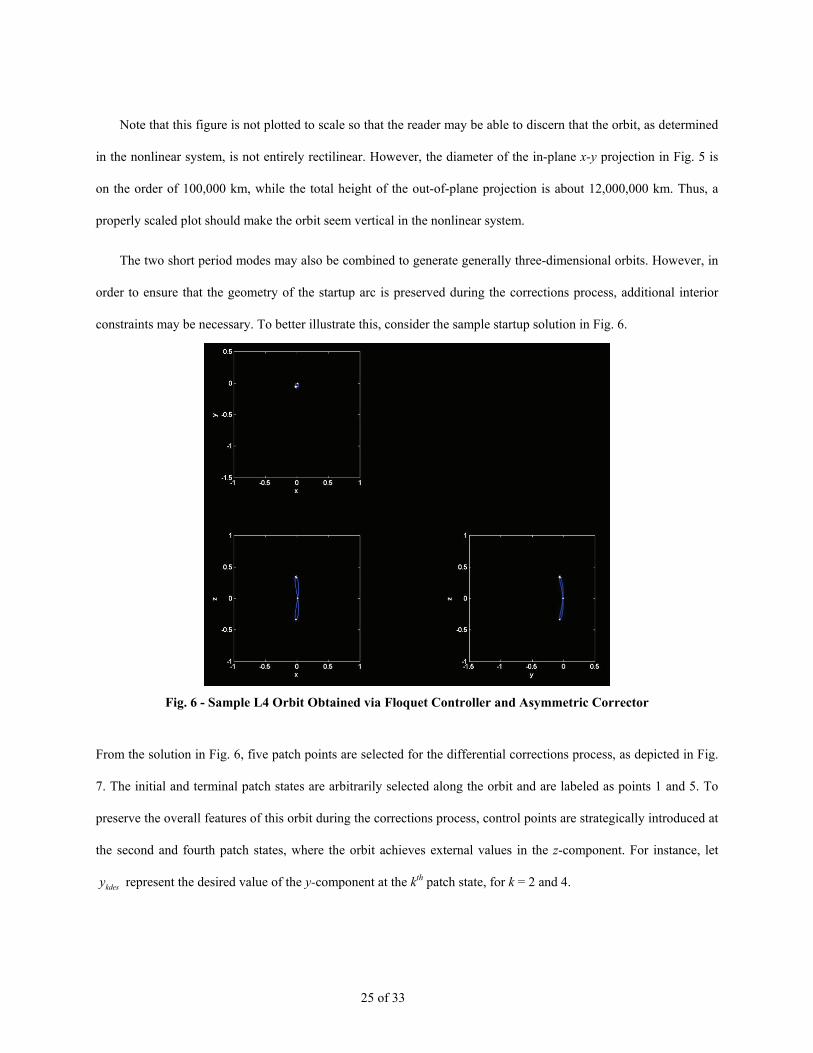
The two short period modes may also be combined to generate generally three-dimensional orbits. However, in

order to ensure that the geometry of the startup arc is preserved during the corrections process, additional interior

constraints may be necessary. To better illustrate this, consider the sample startup solution in Fig. 6.

Fig. 6 - Sample L4 Orbit Obtained via Floquet Controller and Asymmetric Corrector

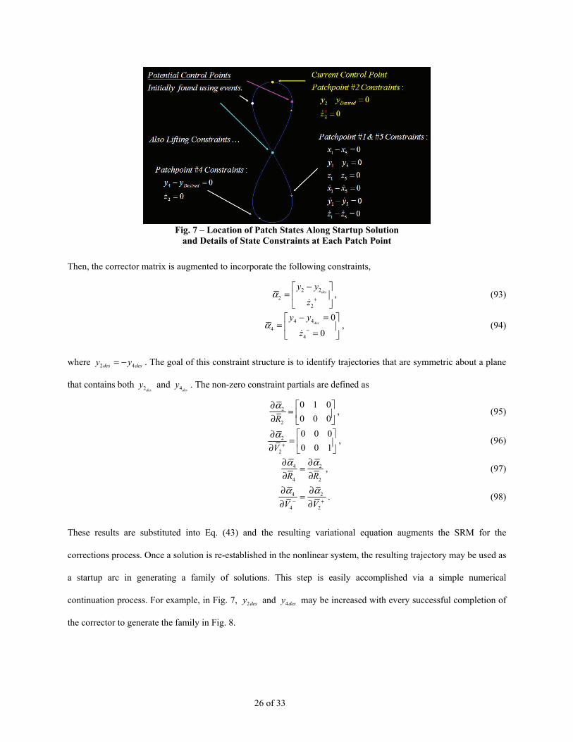
From the solution in Fig. 6, five patch points are selected for the differential corrections process, as depicted in Fig.

7. The initial and terminal patch states are arbitrarily selected along the orbit and are labeled as points 1 and 5. To

preserve the overall features of this orbit during the corrections process, control points are strategically introduced at

the second and fourth patch states, where the orbit achieves external values in the z-component. For instance, let

kdesy represent the desired value of the y-component at the kth patch state, for k = 2 and 4.

26 of 33

Fig. 7 – Location of Patch States Along Startup Solution

and Details of State Constraints at Each Patch Point

Then, the corrector matrix is augmented to incorporate the following constraints,

2 22

2

desy y

zα

+

−⎡ ⎤= ⎢ ⎥⎣ ⎦

, (93)

4 44

4

0

0des

y y

zα

−

− =⎡ ⎤= ⎢ ⎥

=⎣ ⎦, (94)

where 2 4des desy y= − . The goal of this constraint structure is to identify trajectories that are symmetric about a plane

that contains both 2desy and 4des

y . The non-zero constraint partials are defined as

2

2

0 1 00 0 0R

α∂ ⎡ ⎤= ⎢ ⎥∂ ⎣ ⎦

, (95)

2

2

0 0 00 0 1V

α+

∂ ⎡ ⎤= ⎢ ⎥∂ ⎣ ⎦

, (96)

4 2

4 2R Rα α∂ ∂

=∂ ∂

, (97)

4 2

4 2V Vα α

− +

∂ ∂=

∂ ∂. (98)

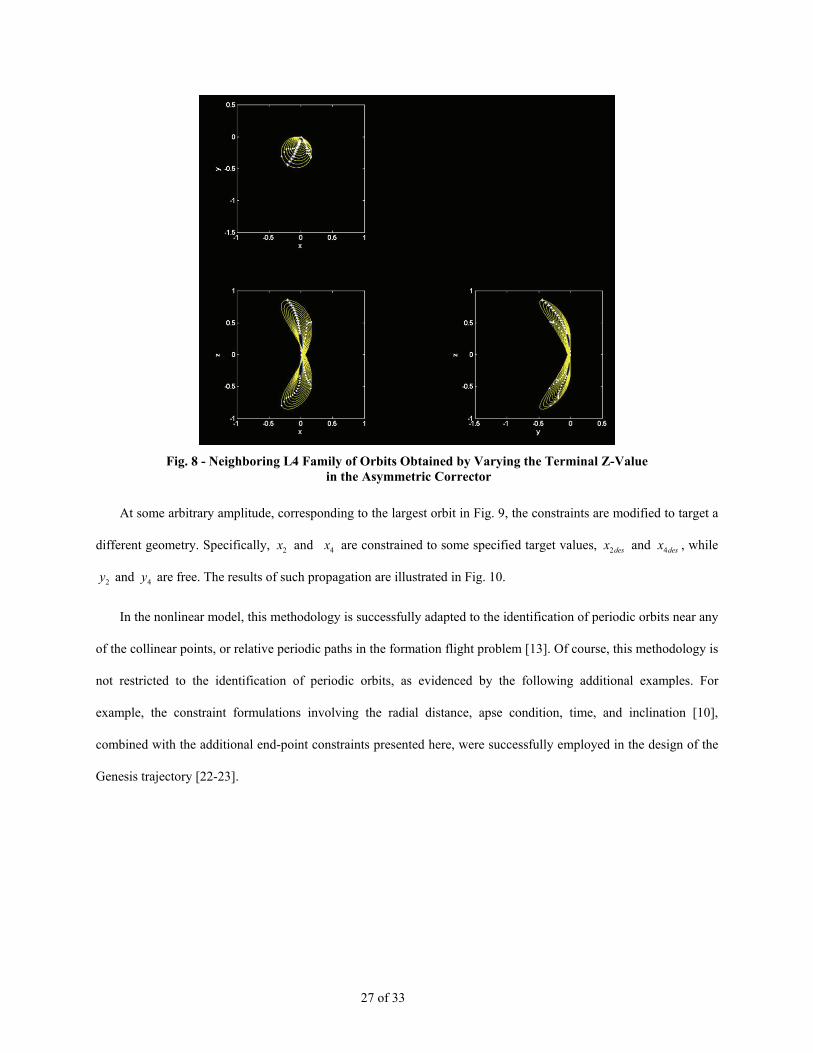
These results are substituted into Eq. (43) and the resulting variational equation augments the SRM for the

corrections process. Once a solution is re-established in the nonlinear system, the resulting trajectory may be used as

a startup arc in generating a family of solutions. This step is easily accomplished via a simple numerical

continuation process. For example, in Fig. 7, 2desy and 4desy may be increased with every successful completion of

the corrector to generate the family in Fig. 8.

27 of 33

Fig. 8 - Neighboring L4 Family of Orbits Obtained by Varying the Terminal Z-Value

in the Asymmetric Corrector

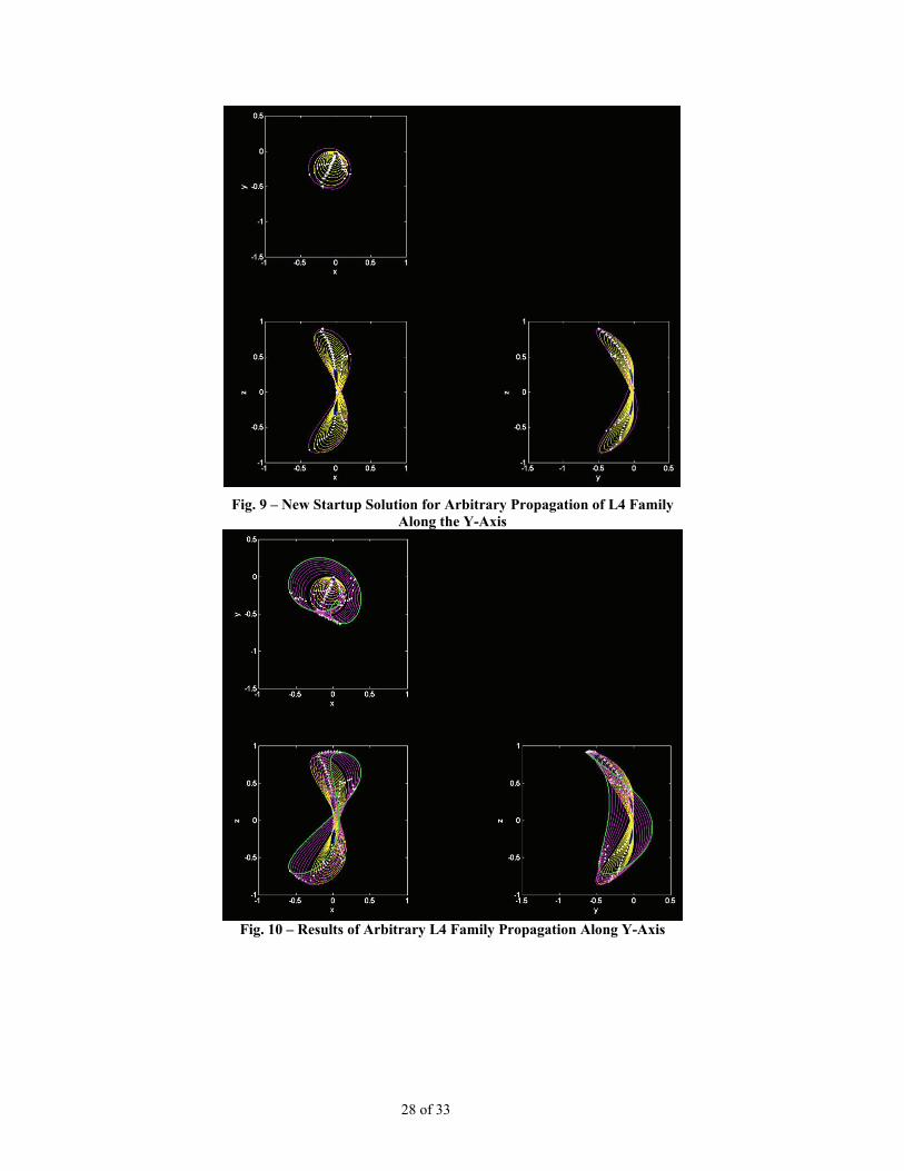
At some arbitrary amplitude, corresponding to the largest orbit in Fig. 9, the constraints are modified to target a

different geometry. Specifically, 2x and 4x are constrained to some specified target values, 2desx and 4desx , while

2y and 4y are free. The results of such propagation are illustrated in Fig. 10.

In the nonlinear model, this methodology is successfully adapted to the identification of periodic orbits near any

of the collinear points, or relative periodic paths in the formation flight problem [13]. Of course, this methodology is

not restricted to the identification of periodic orbits, as evidenced by the following additional examples. For

example, the constraint formulations involving the radial distance, apse condition, time, and inclination [10],

combined with the additional end-point constraints presented here, were successfully employed in the design of the

Genesis trajectory [22-23].

28 of 33

Fig. 9 – New Startup Solution for Arbitrary Propagation of L4 Family

Along the Y-Axis

Fig. 10 – Results of Arbitrary L4 Family Propagation Along Y-Axis

29 of 33

Example #2: Genesis Trajectory Design

In the initial Genesis design [22], originally scheduled for a February 2001 launch as illustrated in Fig. 11, the

corrections process was divided into a launch phase, an orbit phase, and a return phase. However, the methodology

presented here was also successfully applied to an end-to-end design [23], where the launch leg, the lissajous

trajectory, and return leg were simultaneously corrected as a single continuous constrained trajectory in the

ephemeris model. Interior non-zero maneuvers were necessary to meet all the mission constraints. To implement

these maneuvers, the velocity discontinuity constraint at a specific patch point is relaxed by specifying a maximum

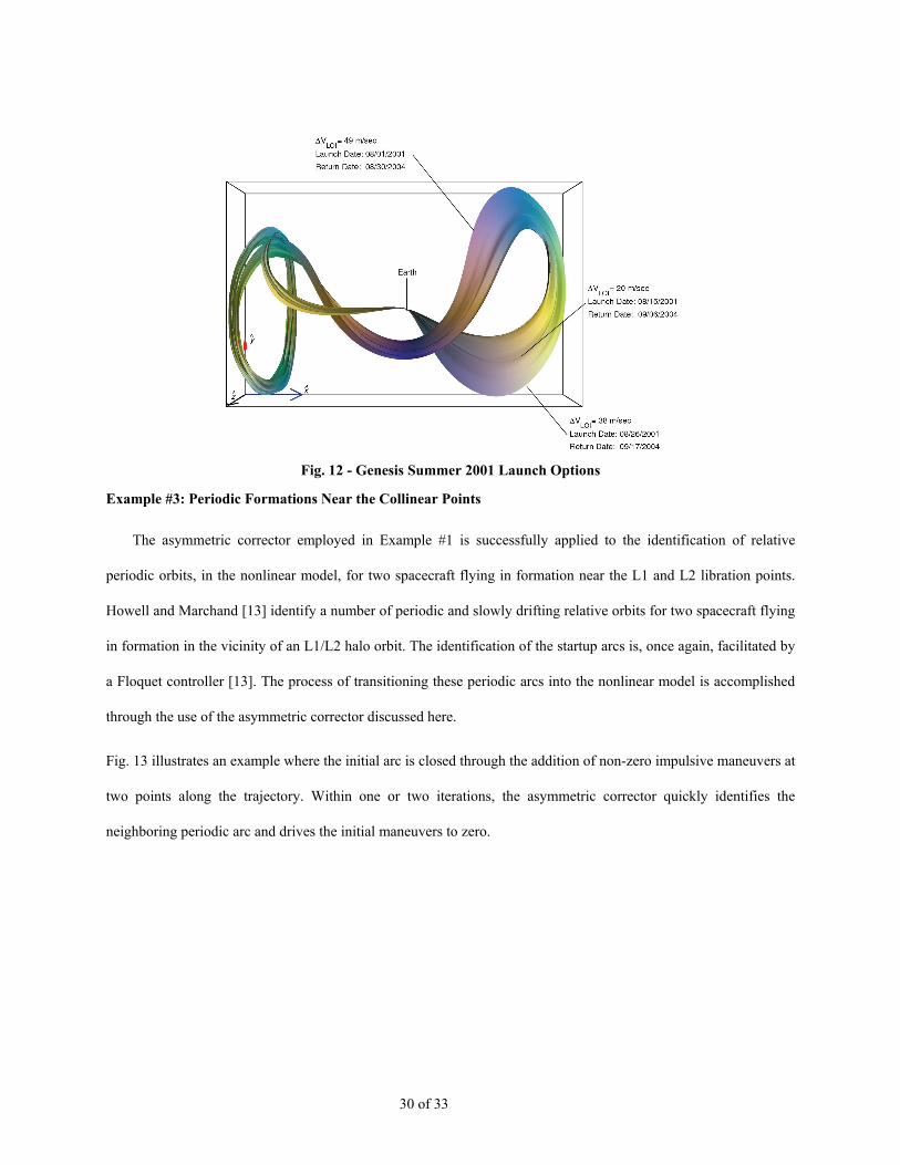
allowable maneuver. The resulting trajectory, for an August-September 2001 launch window, is illustrated in Fig.

12. The surface in Fig. 12 represents a collection of solutions, generated at one day intervals, with radial, apse, and

inclination constraints applied at the launch point, right ascension, declination, radial, and flight path angle

constraints applied at the terminal state, and interior constraints to restrict the magnitude of the maneuvers, including

the Lissajous Orbit insertion maneuver.

Fig. 11 - Initial Genesis Trajectory Design

Figure Courtesy of JPL

30 of 33

Fig. 12 - Genesis Summer 2001 Launch Options

Example #3: Periodic Formations Near the Collinear Points

The asymmetric corrector employed in Example #1 is successfully applied to the identification of relative

periodic orbits, in the nonlinear model, for two spacecraft flying in formation near the L1 and L2 libration points.

Howell and Marchand [13] identify a number of periodic and slowly drifting relative orbits for two spacecraft flying

in formation in the vicinity of an L1/L2 halo orbit. The identification of the startup arcs is, once again, facilitated by

a Floquet controller [13]. The process of transitioning these periodic arcs into the nonlinear model is accomplished

through the use of the asymmetric corrector discussed here.

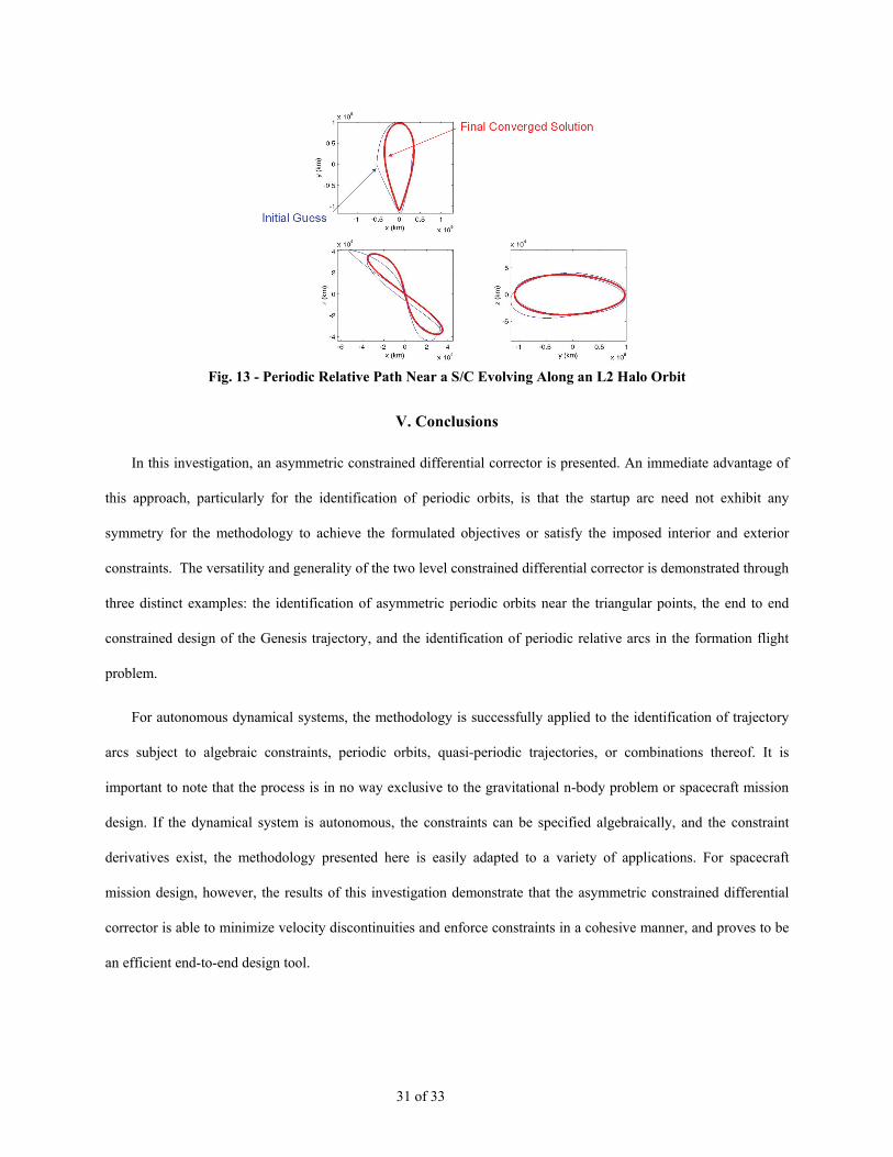
Fig. 13 illustrates an example where the initial arc is closed through the addition of non-zero impulsive maneuvers at

two points along the trajectory. Within one or two iterations, the asymmetric corrector quickly identifies the

neighboring periodic arc and drives the initial maneuvers to zero.

31 of 33

Fig. 13 - Periodic Relative Path Near a S/C Evolving Along an L2 Halo Orbit

V. Conclusions

In this investigation, an asymmetric constrained differential corrector is presented. An immediate advantage of

this approach, particularly for the identification of periodic orbits, is that the startup arc need not exhibit any

symmetry for the methodology to achieve the formulated objectives or satisfy the imposed interior and exterior

constraints. The versatility and generality of the two level constrained differential corrector is demonstrated through

three distinct examples: the identification of asymmetric periodic orbits near the triangular points, the end to end

constrained design of the Genesis trajectory, and the identification of periodic relative arcs in the formation flight

problem.

For autonomous dynamical systems, the methodology is successfully applied to the identification of trajectory

arcs subject to algebraic constraints, periodic orbits, quasi-periodic trajectories, or combinations thereof. It is

important to note that the process is in no way exclusive to the gravitational n-body problem or spacecraft mission

design. If the dynamical system is autonomous, the constraints can be specified algebraically, and the constraint

derivatives exist, the methodology presented here is easily adapted to a variety of applications. For spacecraft

mission design, however, the results of this investigation demonstrate that the asymmetric constrained differential

corrector is able to minimize velocity discontinuities and enforce constraints in a cohesive manner, and proves to be

an efficient end-to-end design tool.

32 of 33

Acknowledgements

The authors extend their appreciation to Daniel Grebow, from Purdue University, for his contributions to the

implementation of Example 1. Portions of this work were completed at Purdue University and The Jet Propulsion

Laboratory.

References

1 Poincaré, H.. “New methods of celestial mechanics: Vol. 1,” American Institute of Physics, New York, 1993. Periodic and asymptotic solutions, Translated from the French, Revised reprint of the 1967 English translation, With endnotes by V. I. Arnold, Edited and with an introduction by Daniel L. Goroff. 2 Farquhar, R.W., Muhonen, D.P., Newman, C.R., Heuberger, H.S., “Trajectories and Orbital Maneuvers for the First Libration-Point Satellite,” Journal of Guidance and Control, Vol. 3, No. 6, 1980, pp. 549-554. 3 Farquhar, R.W., “The Flight of ISEE-3/ICE: Origins, Mission History, and a Legacy,” Journal Astronautical Sciences, Vol. 49, No. 1, 2001, pp. 23-73. 4 Dunham, D. W., Jen, S.J., Roberts, C.E., Seacord, A.W. II, Sharer, P.J., Folta, D.C., and Muhonen, D.P., “Transfer Trajectory Design for the SOHO Libration-Point Mission,” 43rd International Astronautical Congress, IAF Paper 92-0066, Washington, 1992. 5 Stone, E.C., Frandsen, A.M., Mewaldt, R.A., Christian, E.R., Margolies, D., Ormes, J.F., and Snow, F., “The Advanced Composition Explorer,” Space Science Reviews, Vol. 86, 1998, pp. 1-22. 6 Dunham, D.W., Jen, S., Lee, T., Swade, D., Kawaguchi, J., Farquhar, R.W., Broaddus, S., and Engel, C., “Double Lunar-Swingby Trajectories for the Spacecraft of the International Solar-Terrestrial Physics Program,” Advances in the Astronautical Sciences, Vol. 69, 1989, pp. 285-301. 7 Cuevas, O., Kraft-Newman, L., Mesarch, M., and Woodard, M., “An Overview of Trajectory Design Operations for the Microwave Anisotropy Probe Mission,” AIAA/AAS Astrodynamics Specialist Conference and Exhibit, AIAA Paper 2002-4425, AIAA, Monterey, California, 2002. 8 Lo, M., Williams, B., Bollman, W., Han, D., Hahn, Y., Bell, J., Hirst, E., Corwin, R., Hong, P., Howell, K.C., Barden, B., and Wilson, R., “GENESIS Mission Design,” Journal of the Astronautical Sciences, Vol. 49, No. 1, 2001, pp. 169-184. 9 Wilson, R.S., “Trajectory Design in the Sun-Earth-Moon Four Body Problem,” Ph.D. Dissertation, School of Aeronautics and Astronautics, Purdue University, West Lafayette, Indiana, 1998. 10 Wilson, R.S., and Howell, K.C., “Trajectory Design in the Sun-Earth-Moon System Using Lunar Gravity Assists,” Journal of Spacecraft and Rockets, Vol. 35, No. 2, 1998, pp. 191-198. 11 Howell, K.C., “Three-Dimensional Periodic Halo Orbits,” Celestial Mechanics, 1984, Vol. 32, No. 1, pp. 53-71. 12 Markellos, V.V., “The Three-Dimensional General Three-Body Problem: Determination of Periodic Orbits,” Celestial Mechanics, Vol. 21, No. 3, 1980, pp. 291-309. 13 Howell, K.C., and Marchand, B.G., "Natural and Non-Natural Spacecraft Formations Near the L1 and L2 Libration Points in the Sun-Earth/Moon Ephemeris System," Dynamical Systems: an International Journal, Special Issue: "Dynamical Systems in Dynamical Astronomy and Space Mission Design," Vol. 20, No. 1, 2005, pp. 149-173. 14 Richardson, D.L., “Analytic Construction of Periodic Orbits About the Collinear Points.” Celestial Mechanics, Vol. 22, No. 3, 1980, pp. 241-253. 15 Richardson, D.L. and Cary, N.D., “A Uniformly Valid Solution for Motion about the Interior Libration Point of the Perturbed Elliptic-Restricted Problem,” AAS/AIAA Astrodynamics Specialists Conference, AAS Paper No. 75-021, Nassau, Bahamas, 1975.

33 of 33

16 Howell, K.C., Marchand, B.G., and Lo, M.W., “Temporary Satellite Capture of Short-Period Jupiter Family Comets from the Perspective of Dynamical Systems,” The Journal of the Astronautical Sciences, Vol. 49, No. 4, 2001, pp. 539-557. 17 Howell, K.C., and Pernicka, H.J., “Numerical Determination of Lissajous Trajectories in the Restricted Three-Body Problem,” Celestial Mechanics, Vol. 41, No. 1-4, 1987, pp. 107-124. 18 Markellos, V.V., and Halioulias, A.A., “Numerical Determination of Asymmetric Periodic Solutions,” Astrophysics and Space Science, Vol. 46, No. 1., 1977, pp.183-193. 19 Zagouras, C.G., “Three Dimensional Periodic Orbits About the Triangular Equilibrium Points of the Restricted Problem of Three Bodies,” Celestial Mechanics, Vol. 37, No. 1, 1985, pp. 27-46. 20 Papadakis, K.E. and Zagouras, C.G., “Bifurcation Points and Intersections of Families of Periodic Orbits in the Three-Dimensional Restricted Three-Body Problem .” Astrophysics and Space Science, Vol. 199, No. 2, 1993, pp. 241-256. 21 Zagouras, C.G. et al., “New Kinds of Asymmetric Periodic Orbits in the Restricted Three-Body Problem,” Astrophysics and Space Science, Vol. 240, No. 2, 1996, pp. 273-293. 22 Howell, K.C., Barden, B.T., Wilson, R.S., and Lo, M.W., “Trajectory design using a dynamical systems approach with application to GENESIS,” AAS/AIAA Astrodynamics Conference, Sun Valley, Idaho, 1997, pp. 1665-1684. 23 Wilson, R.S., and Barden, B. T., Howell, K.C., and Marchand, B.G. “Summer Launch Options for the Genesis Mission,” Advances in the Astronautical Sciences, Vol. 109, Part 1, 2002, pp. 77-94.