an inhomogeneous landau equation with application to spherical couette flow in the narrow gap limit

Physica D 137 (2000) 260–276

An inhomogeneous Landau equation with application to sphericalCouette flow in the narrow gap limit

Derek Harrisa, Andrew P. Bassomb, Andrew M. Sowarda,∗a School of Mathematical Sciences, University of Exeter, North Park Road, Exeter, Devon EX4 4QE, UK

b School of Mathematics, University of New South Wales, Sydney, NSW 2052, Australia

Received 27 January 1999; received in revised form 6 May 1999; accepted 6 August 1999Communicated by F.H. Busse

Abstract

A nonlinear evolution equation is derived which governs the amplitude modulation of Taylor vortices between two rapidlyrotating concentric spheres which bound a narrow gap and almost co-rotate about a common axis of symmetry. In this weaklynonlinear regime the latitudinal vortex width is comparable to the gap between the shells. The vortices are located close to theequator and are modulated on a latitudinal length scale large compared to the gap width but small compared to the shell radius.The tendency for vortices off the equator to oscillate introduces the phenomenon of phase mixing. Steady finite amplitudesolutions of the model equation are determined both numerically and analytically. The linear eigensolutions are identified byan ascending sequence of eigenvaluesλ = λn (n = 0, 1, . . . ). Each eigensolution has its own finite amplitude continuationunder variation ofλ which is a measure of the excess Taylor number. Without phase mixing each vortex amplitude increasesmonotonically with growingλ and does so indefinitely. In contrast, with phase mixing each pair of linear modes(n = 0, 1),(n = 2, 3), etc. are connected under the finite amplitude continuation; both the mode amplitude andλ remain bounded.Though the small phase mixing results agree with the non-phase mixed ones up to moderately largeλ, this range is of limitedextent. As phase mixing is increased the solution space shrinks and the amplitude of the remaining solutions is stronglysuppressed. ©2000 Elsevier Science B.V. All rights reserved.

Keywords:Landau equation; Couette flow; Taylor vortices

1. Introduction

The flow of incompressible viscous fluid confined between concentric spheres of radiiR1 andR2(> R1), whichrotate about a common axis with angular velocitiesΩ1 andΩ2 respectively, constitutes a fundamental problem influid dynamics. Numerous experimental and computational results have suggested that the transitions between thevarious possible steady state flow configurations are very complicated. Findings reported by Marcus and Tuckerman

∗ Corresponding author.E-mail addresses:[email protected] (D. Harris), [email protected] (A.P. Bassom), [email protected] (A.M. Soward).

0167-2789/00/$ – see front matter ©2000 Elsevier Science B.V. All rights reserved.PII: S0167-2789(99)00181-5

D. Harris et al. / Physica D 137 (2000) 260–276 261

[1,2] indicate that the gap aspect ratioε := (R2 − R1)/R1 is key in determining the character of the instabilitythat sets in when the outer sphere is held at rest while the inner is rotated. For that configuration, they identifynarrow (ε < 0.12), medium(0.12 < ε < 0.24) and wide(0.24 < ε) gap geometries and largely focus theirattention on the medium gap case. For narrow to medium-sized gaps, the undisturbed flow first becomes susceptibleto axisymmetric vortices; they are akin to the ubiquitous Taylor vortices which occur in fluid confined betweena pair of long, concentric circular cylinders. These vortices form in the vicinity of the equator of the sphericalsystem — in some cases these cells have been observed to be symmetric with respect to the equatorial plane whilein other circumstances they are asymmetric [3]. Other work has demonstrated that Taylor vortices are also possiblein large gaps [4]. There is continuing interest in the complicated bifurcation sequence that follows the onset ofinstability particularly in the medium gap case [5].

In the narrow gap limit, Wimmer [6,7] has shown that at the onset of instability axisymmetric Taylor vorticeswith an order one aspect ratio are observed near the equator. This means that the number of vortices between the twospheres at onset increases with decreasingε. Therefore, one might reasonably expect that the instability in the limitε 1 is linked to conditions at the equator, which are adequately modelled by infinite cylinders. This modellingdoes, in fact, capture the main qualitative features but fails to predict the correct onset values in the limiting case.Indeed, Walton [8] appreciated that there was a difficulty with the simplistic cylinder modelling. In consequence, heemployed multiple scale methods based on the idea that the amplitude of the Taylor vortices is modulated betweenthe equator and the pole, with the objective of solving the eigenvalue problem for this modulation. Interestingly,he found that the amplitude equation is influenced by two processes not identified by the cylinder approximation.Not surprisingly, one effect is that of boundary curvature, while the other is the secondary meridional circulationpresent in the basic state (the primary flow being azimuthal). Both lead to the physical mechanism of phase mixingabout which we will expand later. The resulting linear eigenproblem contains several mathematical subtleties whoseresolution eluded the analysis presented in [8–10]. Central to the difficulties encountered was the assumption thatthe critical Taylor numbers for the cylindrical and spherical problems must coincide in the limitε ↓ 0. Later, Sowardand Jones [11] showed this to be an erroneous ansatz and were able to derive the correct asymptotic solution.

Our present objective is to extend the Soward and Jones [11] linear analysis into the weakly nonlinear regime. Itis important at the outset to appreciate that, in addition to the requirement thatε is sufficiently small, our weaklynonlinear study requires that the inner and outer spheres almost co-rotate with large angular velocity(Ω2 − Ω1 Ω1) in a sense made precise by (1.9) below. In this limit our nonlinear amplitude equation coincides with thatappropriate to prolate spheroids [9] without the restriction to almost co-rotation.

Natural parameters which are pertinent in the smallε limit are the Ekman and effective Reynolds numbers

E := ν

R21Ω1 + R2

2Ω2, Ra := ε

ν(R2

1Ω1 − R22Ω2), (1.1a)

whereν denotes the kinematic viscosity of the fluid. HereRa has the appearance of a Reynolds number based on thegap width length scaleR2 − R1 and the angular momentum differenceR2

1Ω1 − R22Ω2. We call it effective because

in our narrow gap application its value may be an order of magnitude different from the true Reynolds number basedon the velocity differenceR1Ω1 − R2Ω2. Soward and Jones [11] characterised the system by the two independentdimensionless parameters:

T := (1 + 12ε)−3ε2E−1Ra, δ := ε−1ERa; (1.1b)

the latter is related to the ratio of the angular momenta of the two shellsµ := R22Ω2/R

21Ω1 by δ ≡ (1−µ)/(1+µ).

The essential idea is that the local solution centred at a co-latitude(π/2) + θ is of separable form with a certainradial structure and a harmonic dependence

exp[i(ε−1kθ − ωt)], (1.2)

262 D. Harris et al. / Physica D 137 (2000) 260–276

in which the wave numberk and frequencyω are generally complex; heret denotes the time. At a given latitude−θ and for given wave numberk and Taylor numberT , the radial structure provides the eigenfunction while thefrequency provides the eigenvalue:

ω = ω (k, θ, T ; δ) +O(ε). (1.3)

In practice, once the values ofω, T andδ have been decided, Eq. (1.3) provides an expression fork = k(θ). In thisway a conventional WKBJ solution can be constructed based on (1.2).

Walton [8] showed that the smallest value ofT for which k is real and−iω has a non-negative real part is astationary modeω = 0 located atθ = 0. Indeed, this is no more than simply the critical value for the correspondingcylinder problem obtained by ignoring curvature effects near the equator. This provides a local stability criterionbut does not determine the ultimate fate of any initial disturbance which can only be resolved by taking accountof the latitudinal dependence ofω. Indeed because of the curvature and meridional circulation mentioned above alocal mode just off the equator has non-zero frequencyω 6= 0. This leads to a mechanism sometimes referred to asphase mixing (see, for example, [12]) and is characterised by a non-zero frequency gradient∂ω/∂θ at the equatorθ = 0. Phase mixing has the effect of shortening the latitudinal length scale and so enhances viscous dissipation.The consequence is that the vortices generated at the cylinder-critical Taylor number are phase mixed and decay.It is perhaps worth remarking that other studies in different parameter ranges have suggested that the meridionalcirculation may play an insignificant role. Even if that is so, curvature alone causes phase mixing, which thereforeoccurs even when meridional motion is ignored. In order to sustain the instability the Taylor number must beincreased by an order one factor above the cylinder-critical value and the realised critical Taylor number is referredto as that appropriate for the global onset of instability.

The correct global stability criteria were given in terms of derivatives ofT = T (k, θ, ω; δ) by Soward and Jones(see Eq. (1.10) and p. 22 of [11]). Expressed in terms of the group velocity and phase mixing, these conditions are

ωk = 0, ωθ = 0, (1.4)

where subscripts denote partial derivatives (see [13]). For axisymmetric Taylor vortices the global conditions (1.4)are satisfied at someT = Tg(δ) by a stationary modeω = 0 characterised by a realk = kg(δ) and purely imaginaryθ = θg(δ).

The underlying basic flow in the spherical shell is best characterised in terms of its angular momentum andmeridional stream function. In general, these quantities exhibit no symmetry about the mean sphere radius(R1 +R2)/2 but, intriguingly, they become symmetric in the constant angular momentum caseRa = 0. In view of (1.1a)this is a singular limit linked toδ ↓ 0. Nevertheless, since the physical processes involved in the absence of phasemixing δ = 0 are simpler, it provides a convenient case about which to pursue a smallδ nonlinear amplitudeexpansion of the solution in the form

a(θ, t) exp(iε−1kg(0)θ) (1.5)

in the neighbourhood of the equator. Herea(θ, t) varies on a length scale long compared to the Taylor cell size butshort compared with the shell radius and it satisfies the inhomogeneous amplitude equation

∂a

∂t= −i

[ωθθ

2θ2 + δωδθ θ + δ2ωδδ

2+ ωT (T − Tg(0))

]a + i

ε2ωkk

2

∂2a

∂θ2. (1.6a)

Here we have noted that

ωδ = 0, ωkδ = 0, ωkθ = 0 (1.6b)


holds, in addition to (1.4), where all partial derivatives ofω are evaluated atk = kg(0), θ = 0 andδ = 0. (The formcorresponding to (1.6a) but expressed in terms of partial derivatives ofT is given by Eq. (3.23) of [11].) Eq. (1.6a)may be scaled to

∂a

∂τ= (λ + 2iκx − x2)a + ∂2a

∂x2(1.7a)

under the change of variables

τ := 12ε(−ωkk ωθθ )

1/2t, x := 1−1/2θ, 1 := ε(ωkk/ωθθ )1/2, (1.7b)

where

κ := iωδθ

ωθθ

δ

11/2, λ := −

(ωδδ

ωθθ

δ2

1+ 2ωT

ωθθ

T − Tg(0)

1

). (1.7c)

For the spherical Couette flow application, Eqs. (3.22) and (3.23) of [11] indicate that both1 andκ are positivenumbers with values

1 ≈ 0.262ε, κ ≈ 0.270δ/ε1/2. (1.8a)

(Note that, in our subsequent analysis, we are less restrictive about the sign ofκ, simply requiring it to be real.)Likewise the expression forλ can be recast in the form

T − Tg(0) ≈ 967λε − 13.0δ2, Tg(0) ≈ 1707.76 (1.8b)

and so the critical value for the onset of instability characterised byλ = λ0 := 1 + κ2 (see (3.1) below) is

Tc ≈ 1707.76+ 57.8δ2 + 967ε (1.8c)

(see Eq. (3.25) of [11]). In the smallε limit, Soward and Jones [11] found that this result was reliable throughoutthe range 0≤ δ ≤ 1, i.e. from the situation of almost co-rotation up to the case of a stationary outer sphere.

Our choice of length scale11/2 = O(ε1/2) in (1.7b) anticipates that the controlling balance in (1.7a) is betweenthe terms−x2a and∂2a/∂x2. Evidently, the phase mixing term 2iκxa is comparable to them whenκ = O(1) or,equivalently, whenδ = O(ε1/2). Since the Taylor number is of order unity this occurs at small Ekman number andlarge effective Reynolds number, specifically

E = O(ε7/4), Ra = O(ε−1/4). (1.9)

Though the parameter range for which the theory is valid is quite tight, we believe that (1.7a) captures importantfeatures of the onset of instability in the narrow gap limit for a wide range of parameters. In particular, the phasemixing element is clearly isolated by the term linear inx while the quadratic component ensures that a point ofvanishing phase mixing can be located atx = iκ, albeit complex.

The first rational treatment of the weakly nonlinear properties of Taylor vortices within concentric cylinder flowswas provided by Davey [14] who derived a standard style Stuart–Landau equation for the scaled disturbance ampli-tude. The development is described in Koschmieder’s [15] book and leads to a supercritical pitchfork bifurcation.In that respect our results for the bifurcation of the lowest mode agree (see (3.2a) and (3.3a)), though for sufficientlylargeκ the bifurcation of the second mode is subcritical (see (3.4a)). It is perhaps worth remarking that Mamun andTuckerman [5] show that the situation for medium gap widths is different with the first bifurcation occuring as asubcritical pitchfork.

The appropriate generalisation of the Stuart–Landau equation to the nearly rigidly rotating spherical flow showsthat the structure of the vortices satisfies the form (1.7a) supplemented by the usual cubic term. Consequently, we


shall devote the remainder of this article to a study of the steady version of (1.7a) with the Stuart–Landau termincluded. The problem reduces to solving

∂a

∂τ= ∂2a

∂x2+ (λ + 2iκx − x2 − |a|2)a with a → 0 as |x| → ∞, (1.10a)

where the boundary conditions have been chosen so as to ensure that the disturbance is trapped within the vicinityof the equator of the system. We will only consider steady solutions∂a/∂τ = 0 and may limit our attention topositivex by seeking solutionsa(x) with the symmetry

a(−x) = a∗(x) so that Re

da

dx(0)

= 0, Ima(0) = 0, (1.10b)

where the asterisk∗ denotes complex conjugate and Re· and Im· denote the real and imaginary parts, respectively.Of course, conditions (1.10b) ensure that Rea is symmetric inx while Ima is antisymmetric. As remarked earlier,Hocking and Skiepko [9] discuss (1.10a) in the context of the instability of flow in the gap between two prolatespheroids. (In their Eq. (A8) on p. 68 of [9], theirτ, α, βy andσ correspond to ourλ, κ, a andΩ; see eq. (4.1)below.) They undertook a preliminary numerical investigation of the nature of the solutions for the particular caseκ = 1.

Our analysis of (1.10) proceeds in the following order. First we deal with the double limit of rapid rotation(E ↓ 0)

but almost uniform angular momentum(Ra ↓ 0), with finite Taylor numberT (see (1.1a) and (1.1b)). Thenµ = 1so thatδ = 0 and (1.7c) givesκ = 0. Hence we lose the imaginary term in (1.10a) and what remains is discussedin Section 2. Though the results for this case are relatively straightforward (see also [9]), they provide an essentialbench mark against which the results forκ 6= 0 can be compared. That more complicated case is attacked in Section3 using a mixture of analytical and numerical methods. We find that the salient features found in the preliminarynumerical study by Hocking and Skiepko [9] for the particular caseκ = 1 continue to hold for other values ofκ.Our main achievement is this overview supported by the insight gained from the asymptotics, namely the weaklynonlinear results and our analytic solutions for small and largeκ; together they build a remarkable picture. Finally,we close in Section 4 with a short discussion of our findings.

2. Equal angular momenta limit: κ = 0

We begin by considering system (1.10) when the coefficientκ vanishes. The remaining coefficients in the differ-ential equation are all real-valued and the task of studying the solutions is relatively elementary. In the case of smallamplitude vortices, we can effectively drop the cubic term in the equation and we are simply left with a scaled versionof the standard parabolic cylinder equation [16]. Bounded solutions exist forλ = λn := 1 + 2n, n = 0, 1, 2, . . . :solutions withn even (odd) are themselves symmetric (antisymmetric) functions ofx. In most circumstances wewould expect the solutions with smalln to be the physically significant ones as these are associated with the smallervalues ofλ (and hence the smaller values for elevation of Taylor number aboveTg(0), see (1.7c)). Consequently wenote that the first even (symmetric) and first odd (antisymmetric) solutions of the linearised version of (1.10a) withκ = 0 have the formsa0(x) = β exp(−x2/2) (n = 0) anda1(x) = iβx exp(−x2/2) (n = 1) respectively, whereby our symmetry convention (1.10b) the arbitrary constantβ is real.

An application of standard nonlinear ideas makes it straightforward to ascertain the effect of nonlinearity as theamplitude of the vortices is slowly increased. So for example, withn = 0, we adoptβ as our small expansionparameter, set

a = β(1 + β2u(x))exp(−12x2) and λ − 1 = β2λ0 1, (2.1)


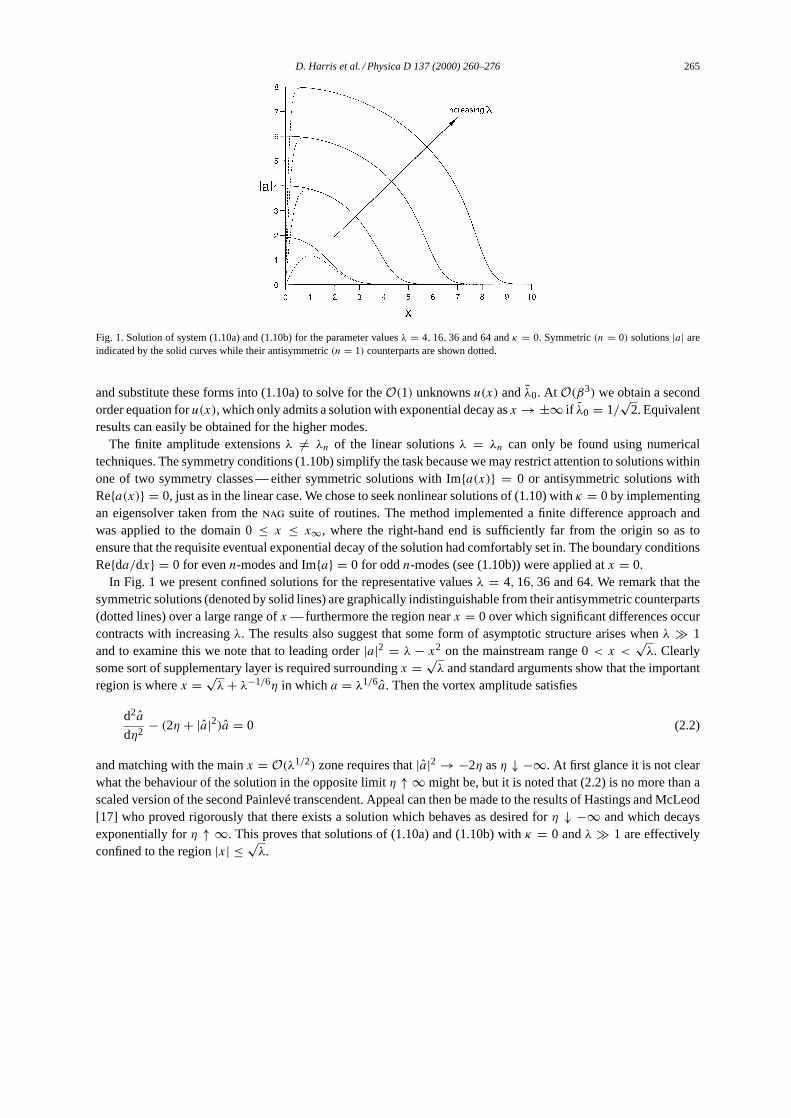
Fig. 1. Solution of system (1.10a) and (1.10b) for the parameter valuesλ = 4, 16, 36 and 64 andκ = 0. Symmetric(n = 0) solutions|a| areindicated by the solid curves while their antisymmetric(n = 1) counterparts are shown dotted.

and substitute these forms into (1.10a) to solve for theO(1) unknownsu(x) andλ0. At O(β3) we obtain a secondorder equation foru(x), which only admits a solution with exponential decay asx → ±∞ if λ0 = 1/

√2. Equivalent

results can easily be obtained for the higher modes.The finite amplitude extensionsλ 6= λn of the linear solutionsλ = λn can only be found using numerical

techniques. The symmetry conditions (1.10b) simplify the task because we may restrict attention to solutions withinone of two symmetry classes — either symmetric solutions with Ima(x) = 0 or antisymmetric solutions withRea(x) = 0, just as in the linear case. We chose to seek nonlinear solutions of (1.10) withκ = 0 by implementingan eigensolver taken from thenag suite of routines. The method implemented a finite difference approach andwas applied to the domain 0≤ x ≤ x∞, where the right-hand end is sufficiently far from the origin so as toensure that the requisite eventual exponential decay of the solution had comfortably set in. The boundary conditionsReda/dx = 0 for evenn-modes and Ima = 0 for oddn-modes (see (1.10b)) were applied atx = 0.

In Fig. 1 we present confined solutions for the representative valuesλ = 4, 16, 36 and 64. We remark that thesymmetric solutions (denoted by solid lines) are graphically indistinguishable from their antisymmetric counterparts(dotted lines) over a large range ofx — furthermore the region nearx = 0 over which significant differences occurcontracts with increasingλ. The results also suggest that some form of asymptotic structure arises whenλ 1and to examine this we note that to leading order|a|2 = λ − x2 on the mainstream range 0< x <

√λ. Clearly

some sort of supplementary layer is required surroundingx = √λ and standard arguments show that the important

region is wherex = √λ + λ−1/6η in whicha = λ1/6a. Then the vortex amplitude satisfies

d2a

dη2− (2η + |a|2)a = 0 (2.2)

and matching with the mainx = O(λ1/2) zone requires that|a|2 → −2η asη ↓ −∞. At first glance it is not clearwhat the behaviour of the solution in the opposite limitη ↑ ∞ might be, but it is noted that (2.2) is no more than ascaled version of the second Painlevé transcendent. Appeal can then be made to the results of Hastings and McLeod[17] who proved rigorously that there exists a solution which behaves as desired forη ↓ −∞ and which decaysexponentially forη ↑ ∞. This proves that solutions of (1.10a) and (1.10b) withκ = 0 andλ 1 are effectivelyconfined to the region|x| ≤ √

λ.


This leading order solution is evidently symmetric aboutx = 0 so the lowest order antisymmetric solution requiressome additional structure to be imposed. This is also apparent on Fig. 1 and corresponds to the thin zone surroundingx = 0, wherein the main difference between the antisymmetric and symmetric solutions exists. A simple analysisshows that, in this internal boundary layer, the antisymmetric solution is given bya = i

√λ tanh

(x√

λ/2), for x =

O(λ−1/2). Evidently this form possesses the requisite symmetry properties and matches onto the mainstream solutionwhen x = O(λ1/2). Good agreement exists between this small-x asymptote and the corresponding numericalsolutions portrayed in Fig. 1.

It should be pointed out that each linear parabolic cylinder function modean(x) (see (3.1)) below withκ = 0)has its finite amplitude extension, which remains symmetric (antisymmetric) forn even (odd). For large values ofλ but moderaten their mainstream solutions are still given by|a|2 = λ − x2 correct to leading order. The onlydifference lies in the structure of the internal boundary layer, where all the oscillatory structure is confined. Thelayer containsn zeros and thickens with increasingn. Since the key features of the finite amplitude solutions areillustrated well by the symmetric evenn = 0 and antisymmetric oddn = 1 modes, we restrict attention to these inour analysis of the phased mixed extensions in the following section.

3. Phase mixed vorticesκ 6= 0

We begin our investigation of the full form of (1.10a) by considering its linearised solutions. In a manneridentical to that for theκ = 0 problem it is simple to transform the governing equation into the standard paraboliccylinder function equation. The demand that we have bounded solutions leads to the permissible valuesλ = λn :=1 + κ2 + 2n, n = 0, 1, . . . with linearised eigensolutions, possessing the symmetry (1.10b), of the form

an(x) := inβU(−n − 12,

√2(x − iκ)) for κ > 0, (3.1)

whereU denotes the usual parabolic cylinder function [16] andβ is an arbitrary real constant.Since the non-zeroκ modes are fully complex they possess both symmetries and so the characterisation of

symmetric and antisymmetric is inappropriate. Since, however, the linear modes are identified by even or oddn, wecall their nonlinear extensions even and odd also. A minor complication arises with this nonlinear categorisation,because we find that even modes are connected to odd modes in parameter space. Nevertheless, our usage of theterms even and odd should become quite transparent.

3.1. Weakly nonlinear theory for|λ − λn| 1

The weakly nonlinear extension of these results is derived by the normal procedure. As in (2.1), we consider theexpansion

a = (1 + β2u(x))an(x), where β2 := (λ − λn)/λn 1 . (3.2a)

Hereλn is determined (so fixingβ) by the consistency condition that upon substitution into (1.10a) and (1.10b) abounded solution is possible atO(β3). That occurs if and only ifλn satisfies

λn

∫ ∞

−∞a2n dx =

∫ ∞

−∞|an|2a2

n dx. (3.2b)

It is instructive to evaluate these integrals in the case of the dominant even(n = 0) and odd(n = 1) modes. Inthe former(n = 0) case it is found that


λ0 = 1√2

exp(32κ2), (3.3a)

from which we deduce

da0

dx(0) = iκ a0(0) with |a0(0)|2 =

√2(λ − λ0)exp(−1

2κ2). (3.3b)

In the latter(n = 1) case, we obtain

λ1 = 3

8√

2(1 + 2κ2 − κ4)exp(3

2κ2), (3.4a)

which leads to the result

da1

dx(0) = i(1 + κ2)

a1(0)

κwith

∣∣∣∣a1(0)

κ

∣∣∣∣2

= 8√

2(λ − λ1)

3(1 + 2κ2 − κ4)exp(−1

2κ2). (3.4b)

Once more it is theoretically possible, although algebraically very tedious, to derive equivalent correction terms forthe higher order modes. However it is of interest to contrast the behaviours of (3.3), (3.4). It is clear from (3.3) thatthe zeroth-mode is supercritical irrespective of the value ofκ while the first mode with amplitude given by (3.4b)is supercritical forκ2 < 1 + √

2 but subcritical for larger values. We shall see evidence of this switch in stabilityin our numerical solutions discussed below.

An unfortunate feature of (3.2a) is that the correctionβ2u to the amplitude modulation is not uniformly smalland becomes large as|x| → ∞. A better representation of the linear solutiona(x) for |x| 1 is

Ak(x) := iαβ Uk(−α − 12,

√2ζ ) for κ > 0, (3.5a)

where

α := (λ − 1 − κ2)/2 , ζ := x − iκ, (3.5b)

and

Uk

(−α − 1

2,√

2ζ)

:= (√

2ζ )α[1 − α(α − 1)

4ζ 2+ . . .

]exp(−1

2ζ 2) (3.5c)

is the large positiveζ -asymptotic expansion of the parabolic cylinder functionU truncated at the(k + 1)th term(k = 0, 1, . . . ). It is important to appreciate thatAk(x), though motivated by its large positivex behaviour, is acontinuous function for all realx provided thatκ 6= 0. Furthermore, our choice of normalisation ensures thatAk(x)

meets the symmetry condition (1.10b) and so can be used to give the large negativex asymptotic representation ofa(x) also.

The reason for the retention of preciselyk +1 terms stems from the fact thatAk(x) gives the exact linear solutionof (1.10a) when eitherλ = λ2k or λ = λ2k+1 and can be used as the basis of a small amplitude expansion ofa(x)

for λ in the neighbourhood of those values. Let us consider the first pairλ0 andλ1 corresponding tok = 0. Uponmultiplying (1.10a) byA0(x) and integrating over allx, we obtain

α(α − 1)

∫ ∞

−∞aA0

(x − iκ)2dx =

∫ ∞

−∞|a|2aA0 dx. (3.6)

Now if we approximate the weakly nonlinear solutions by

a(x) ≈ a(0)A0(x)/A0(0) , (3.7a)


integration of (3.6) yields

π α(1 − α)

0(32 − α)

≈ |a(0)|2exp(12κ2)

∫ ∞

−∞

(x2 + κ2

κ2

)α

[i (x − iκ)]2α exp[−2(x − iκ/2)2

]dx. (3.7b)

The evaluation of the integral on the right-hand side atα = 0 andα = 1 recovers our earlier results (3.3b) and(3.4b), respectively.

The power of the present approach only becomes apparent whenκ is large. Then we may evaluate the integral in(3.7b) asymptotically for arbitrary positiveα to obtain

|a(0)|2 ≈ α(1 − α)

(4√3|κ|

)2α√

2π

0(32 − α)

exp(−12κ2) for |κ| 1. (3.8)

Since this predicts exponentially small amplitudes we may reasonably expect the WKBJ type solutions (3.5a) to bevalid for all realx. Nevertheless, the linear system is extremely fragile due to the fact that its double turning pointx = iκ is far from the realx-axis. The usefulness of the formula (3.7b) depends on the the closeness ofa(x) toA0(x). Since the saddle pointx = iκ/2 of the integral on the right-hand side of (3.7b) is located solidly in a regionwhere|a − A0| is likely to be exponentially small, we may anticipate that the value given by that integral of thenonlinear contribution is reasonably robust. That is not the case for the integral of the linear term contribution on theleft-hand side, because the saddle point contribution occurs at the double turning pointx = iκ, where|a −A0| is nolonger exponentially small (although exactly how small it is remains unclear). Interestingly however, our numericalresults portrayed in Fig. 6 below forκ = 4 compare extremely well with (3.8) over the entire intervalλ0 ≤ λ ≤ λ1.

Despite the encouraging nature of the numerical comparison onλ0 ≤ λ ≤ λ1, the formula (3.8) based onA0(x)

does not give useful approximations elsewhere. This observation is in accord with the remarks just made. We mayreasonably anticipate that on each successiveλ-intervalλ2k ≤ λ ≤ λ2k+1 the functionAk(x) gives a more reliablerepresentation ofa(x) in the important vicinity of the double turning point. Accordingly we propose that (1.10a)is multiplied byAk(x) and integrated over allx to obtain an approximate result comparable to (3.8). Though thisconstruction necessarily gives good results in the weakly nonlinear regimes near the end pointsλ2k andλ2k+1, thereis no guarantee that the approximate results will be as accurate elsewhere in the interval.

3.2. Large amplitude theory for|λ − λn| 1: weak phase mixing|κ| 1

A last area in which some analytical progress is possible concerns that of near equal angular momenta of the twoshells in our spherical system so that the parameterκ is small. Guided by the asymptotic analysis of Section 2 it iseasiest to isolate the dominant nonlinear mainstream behaviour by introducing a polar representation and changeof variables

λ − x2 = κ−2ξ, λ = κ−23, a = κ−1Φ exp

[i

((sgnκx)ϕ∞ + κ−1

∫ x

0K dx

)], (3.9)

whereΦ andK are real even functions ofx andϕ∞ is included in anticipation of a possible phase shift across aninternal boundary layer in the neighbourhood ofx = 0. With these substitutions system (1.10a) becomes

κ4(

4(3 − ξ)d2Φ

dξ2− 2

dΦ

dξ

)+ (ξ − K2 − Φ2)Φ = 0, (3.10a)

d

dξ(KΦ2) − Φ2 = 0 (3.10b)


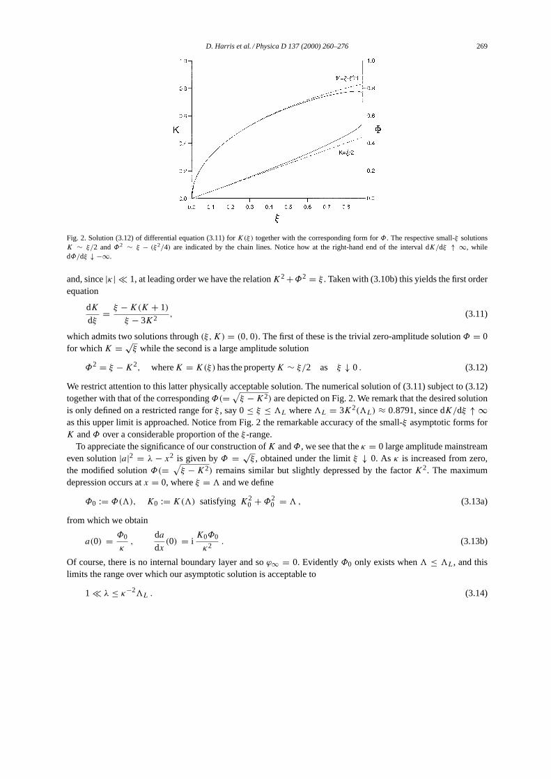
Fig. 2. Solution (3.12) of differential equation (3.11) forK(ξ) together with the corresponding form forΦ. The respective small-ξ solutionsK ∼ ξ/2 andΦ2 ∼ ξ − (ξ2/4) are indicated by the chain lines. Notice how at the right-hand end of the interval dK/dξ ↑ ∞, whiledΦ/dξ ↓ −∞.

and, since|κ| 1, at leading order we have the relationK2 +Φ2 = ξ . Taken with (3.10b) this yields the first orderequation

dK

dξ= ξ − K(K + 1)

ξ − 3K2, (3.11)

which admits two solutions through(ξ, K) = (0, 0). The first of these is the trivial zero-amplitude solutionΦ = 0for whichK = √

ξ while the second is a large amplitude solution

Φ2 = ξ − K2, whereK = K(ξ) has the propertyK ∼ ξ/2 as ξ ↓ 0 . (3.12)

We restrict attention to this latter physically acceptable solution. The numerical solution of (3.11) subject to (3.12)together with that of the correspondingΦ(=

√ξ − K2) are depicted on Fig. 2. We remark that the desired solution

is only defined on a restricted range forξ , say 0≤ ξ ≤ 3L where3L = 3K2(3L) ≈ 0.8791, since dK/dξ ↑ ∞as this upper limit is approached. Notice from Fig. 2 the remarkable accuracy of the small-ξ asymptotic forms forK andΦ over a considerable proportion of theξ -range.

To appreciate the significance of our construction ofK andΦ, we see that theκ = 0 large amplitude mainstreameven solution|a|2 = λ − x2 is given byΦ = √

ξ , obtained under the limitξ ↓ 0. As κ is increased from zero,the modified solutionΦ(=

√ξ − K2) remains similar but slightly depressed by the factorK2. The maximum

depression occurs atx = 0, whereξ = 3 and we define

Φ0 := Φ(3), K0 := K(3) satisfying K20 + Φ2

0 = 3 , (3.13a)

from which we obtain

a(0) = Φ0

κ,

da

dx(0) = i

K0Φ0

κ2. (3.13b)

Of course, there is no internal boundary layer and soϕ∞ = 0. EvidentlyΦ0 only exists when3 ≤ 3L, and thislimits the range over which our asymptotic solution is acceptable to

1 λ ≤ κ−23L . (3.14)


By direct analogy with theκ = 0 odd solutions, we consider the appropriate extension

a = κ−1Φ exp

[i(sgnκ)

∫ X

0K dX

](X = x/|κ|) (3.15)

of the boundary layer structure in the neighbourhood of the originx = 0 on the short length scaleκ. There theequation equivalent to (3.10a) and (3.10b) forΦ(X) andK(X) takes the form

d2Φ

dX2+ (3 − κ4X2 − K2 − Φ2)Φ = 0 , (3.16a)

d

dX(KΦ2) + 2κ4XΦ2 = 0 . (3.16b)

Under this scaling the terms of sizeO(κ4) are negligible. The integration of (3.16b) subject to matching asX ↑ ∞givesKΦ2 = K0Φ

20. Using this result, we can solve (3.16a) subject to matching and so obtain

Φ2 = 2K20 + (3 − 3K2

0) tanh2

√3 − 3K2

0

2X

, (3.17a)

K = K0Φ20/Φ2 ,

∫ X

0(K − K0) dX = ϕ , (3.17b)

where

tanϕ =√

3 − 3K20

2K20

tanh

√3 − 3K2

0

2X

. (3.17c)

Hence the phase shift in the mainstream solution (3.9) across half the internal boundary layer is

ϕ∞ = tan−1

√3 − 3K2

0

2K20

, (3.17d)

and these results yield

a(0) =√

2K20

κ,

da

dx(0) = i

Φ20√

2κ2. (3.17e)

In the3 ↓ 0 limit we haveK0/Φ0 ↓ 0 and so can clearly identify from the above results the large amplitude oddsolution of the previous section including the factor “i” which results from the phase shiftϕ∞ = π/2 across halfthe internal boundary layer. As3 increases,ϕ∞ decreases monotonically to zero at3 = 3L, where3− 3K2

0 = 0.Simultaneously, the strength of the internal boundary layer collapses. Indeed, the values ofa(0) and da/dx(0) givenby the even (3.13b) and odd (3.17e) branches coincide at3 = 3L. These features are confirmed by the numericalsolutions discussed next.

3.3. Numerical solutions

In order to explore other parameter regimes for Eq. (1.10a) we were forced to resort to a numerical approach. Wesolved the governing system using the same kind of nonlinear eigenvalue solver mentioned earlier and could oncemore restrict our attention to the half-space 0≤ x < ∞ with the symmetry conditions (1.10b) applied atx = 0.


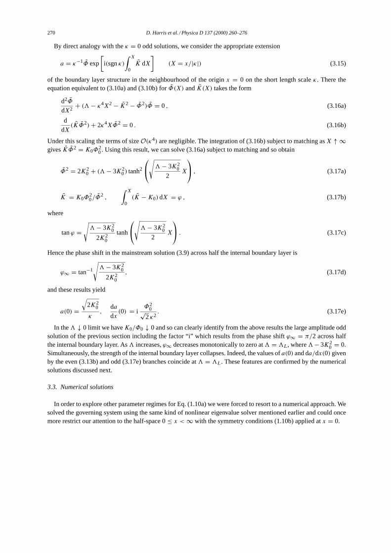
Fig. 3. |a(0)| versusλ for various values ofκ. (a) The numerical results are shown forλ = O(κ−2). The continuous (broken) curves illustratethe numerical solutions of (1.10a) and (1.10b) on the even (odd) branch of the lobe emerging fromλ = λ0 (λ = λ1). (b) Forλ = O(κ−2)

the numerical results are identified as in (a), while the dotted curves from the origin illustrate the asymptotic results (3.13b) and (3.17e) asdetermined via (3.13a).

We adopt two measures of the amplitude of our solution, namely|a(0)| and|da/dx(0)|. Their dependence onλ is illustrated in Figs. 3 and 4, respectively, for a selection of fixed smallκ values. The reason for introducingtwo measures is suggested by theκ = 0 modes with pure symmetry: either|da/dx(0)| = 0 for the symmetriceven modes, or|a(0)| = 0 for the antisymmetric odd modes. These trivial zero measures are unhelpful and onlythe other (non-trivial) measure is useful. Accordingly, for thisκ = 0 case, the lowest symmetric even(n = 0)

mode, measured by|a(0)|, is illustrated in Fig. 3(a). It emerges from the linear solution atλ0 = 1 with thesmall amplitude behaviour|a0(0)| ∼ 21/4(λ − 1)1/2, approaches the asymptote|a(0)| ∼ √

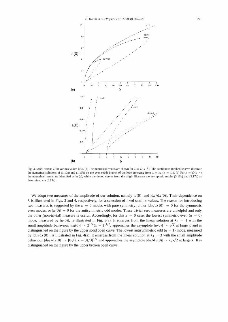
λ at largeλ and isdistinguished on the figure by the upper solid open curve. The lowest antisymmetric odd(n = 1) mode, measuredby |da/dx(0)|, is illustrated in Fig. 4(a). It emerges from the linear solution atλ1 = 3 with the small amplitudebehaviour|da1/dx(0)| ∼ [8

√2(λ − 3)/3]1/2 and approaches the asymptote|da/dx(0)| ∼ λ/

√2 at largeλ. It is

distinguished on the figure by the upper broken open curve.


Fig. 4.|da/dx(0)| versusλ for various values ofκ. (a) As in Fig. 3(a). (b) As in Fig. 3(b).

We notice a significant change of behaviour onceκ is non-zero; Figs. 3(a) and 4(a) show that there is a well-definedmaximum amplitude beyond which our nonlinear solutions are not possible. This feature was also identified byHocking and Skiepko’s [9]κ = 1 results listed in their Table 3. Significantly, the modes no longer possess the puresymmetry described above and soa(0) 6= 0 and da/dx(0) 6= 0 simultaneously. Accordingly, for givenκ 6= 0, thefirst two linear solutions (3.1)(n = 0) and(n = 1) emerge from theλ-axis atλ0 := 1 + κ2 andλ1 := 3 + κ2,respectively and now have non-zero measures visible in both Figs. 3(a) and 4(a). On theλ = O(κ−2) scale ofthese figures, the solid curves produced by the numerics are indistinguishable from that predicted by the even modeasymptotic results (3.13b) of Section 3.2 up to graph plotting accuracy, except for relatively smallλ = O(1).Likewise, the odd mode asymptotic results (3.17e) almost coincide with the broken curves over the entire rangealso. In this way, we see from Fig. 3(a) that|a(0)| for these two modes is connected sequentially by an open lobefollowed in a clockwise sense, while the lobe for|da/dx(0)| in Fig. 4(a) is followed in an anticlockwise sense.Note that here the lobe is not open but exhibits a curve crossing atλ ≈ 3 (Fig. 4(b), but see the description ofit below).


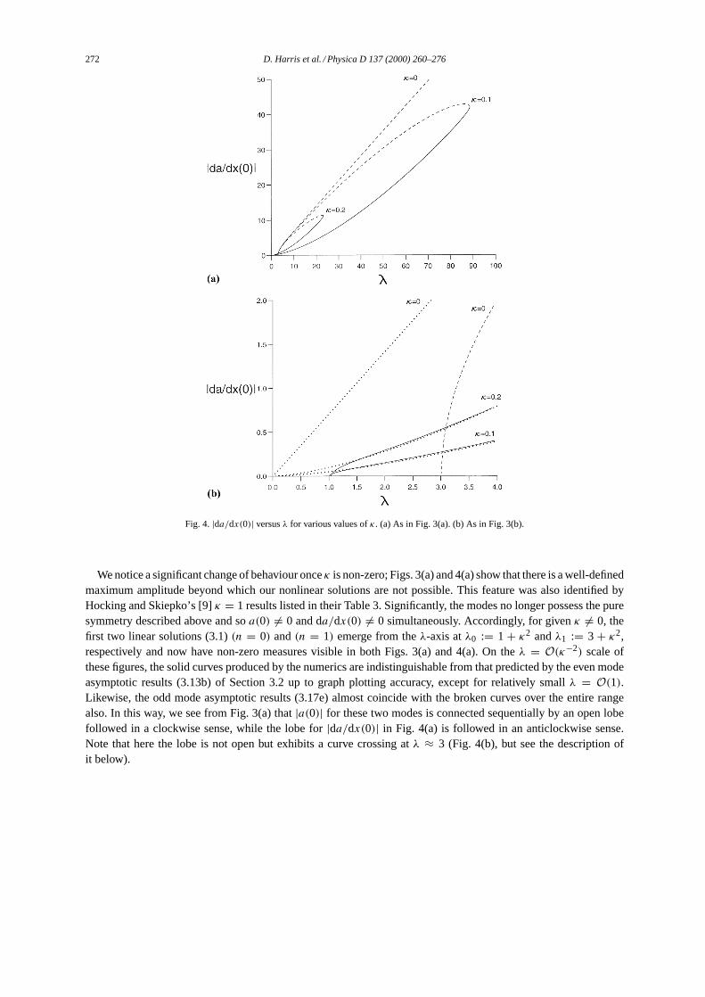
Fig. 5. The numerically computed finite amplitude solutions as represented by the polar form (3.15). The first even (solid curves) and odd (brokencurves) modes are illustrated forλ = 4, 16, 36, 64 with κ = 0.1. (a)κ−1Φ versusx. The amplitudeκ−1Φ = |a(0)| at the origin is given bythe data portrayed on Fig. 3(a) and identified by the corresponding solid and broken curves; (b)κ−1K versusx.

The departure of the numerical results from the asymptotic predictions (3.13b) and (3.17e) of Section 3.2 areillustrated forλ = O(1) in Figs. 3(b) and 4(b). There the numerical results are readily distinguished for whereasthey leave theλ-axis at non-zeroλ0 andλ1, the asymptotic results stem from the originλ = 0. Interestingly, thetrivial κ = 0 zero measures fan out in a clearly visible way forκ = 0.1 and 0.2. In contrast, the non-trivialκ = 0measures hardly alter and these curves forκ = 0, 0.1 and 0.2 are indistinguishable to graph plotting accuracy.Evidently, the asymptotic results give a good description of the numerical solutions almost everywhere; where themeasures break away at smallλ − λn (identified by the trivialκ = 0 case) the weakly nonlinear results of Section3.1 give better approximations.

The numerical results were generated by solving (3.3) for the coordinates(κ−1Φ, κ−1K) of the polar represen-tation (3.15) of the complex amplitude. The computed values ofκ−1Φ = |a(x)| andκ−1K at various values ofλ are plotted versusx = |κ|X in Figs. 5(a) and (b), respectively. The solid curves denote the even solutions withno internal boundary layer. Throughout the mainstream(x √

λ) they agree well with the asymptotic results for


κ−1Φ(ξ) andκ−1K(ξ), which use the data illustrated in Fig. 2. As expected, however, they differ significantlyacross the transitional layer atx = √

λ, which is again governed by (2.2). The odd solutions (at the sameλ-values)coincide with the even solutions, except within the internal boundary layer(x = O(κ)). There they are identifiedby the broken lines, which are approximated well by (3.17). The strength of the boundary layer, as measured bythe differenceκ−11Φ between the values of|a(0)| for the even and odd modes, is given by the asymptotic result

1Φ = Φ0 − Φ(0) =√

3 − K20 −

√2K2

0 derived from (3.17) whenλ = O(κ−2). The differenceκ−11Φ isessentially the gap between the upper and lower branches of the lobe illustrated in Fig. 3(a) and, asλ increases up toκ−23L, this gap width collapses to zero whereupon the distinction between even and odd modes evaporates. Thisdiminishing of boundary layer strength is also evident in Fig. 5(a).

Figs. 3 and 4 have shown how the nonlinear solutions of system (1.10) can be thought of as connecting thezeroth and first order linearised solutions (3.1). Further computations show that additional branches of nonlinearsolutions connect the(2k)th and(2k + 1)th linearised forms (k = 1, 2, . . . ) and such solutions intersect theλ-axisat λ2k = (4k + 1) + κ2 andλ2k+1 = (4k + 3) + κ2. Thus the full picture of nonlinear solutions for a chosenκ

consists of a whole string of lobes which emanate from well-defined positions on theλ-axis. However the maximumsolution amplitudes fall off extremely rapidly with distance along theλ-axis and so are unlikely to be the principalforms of vortex mode.

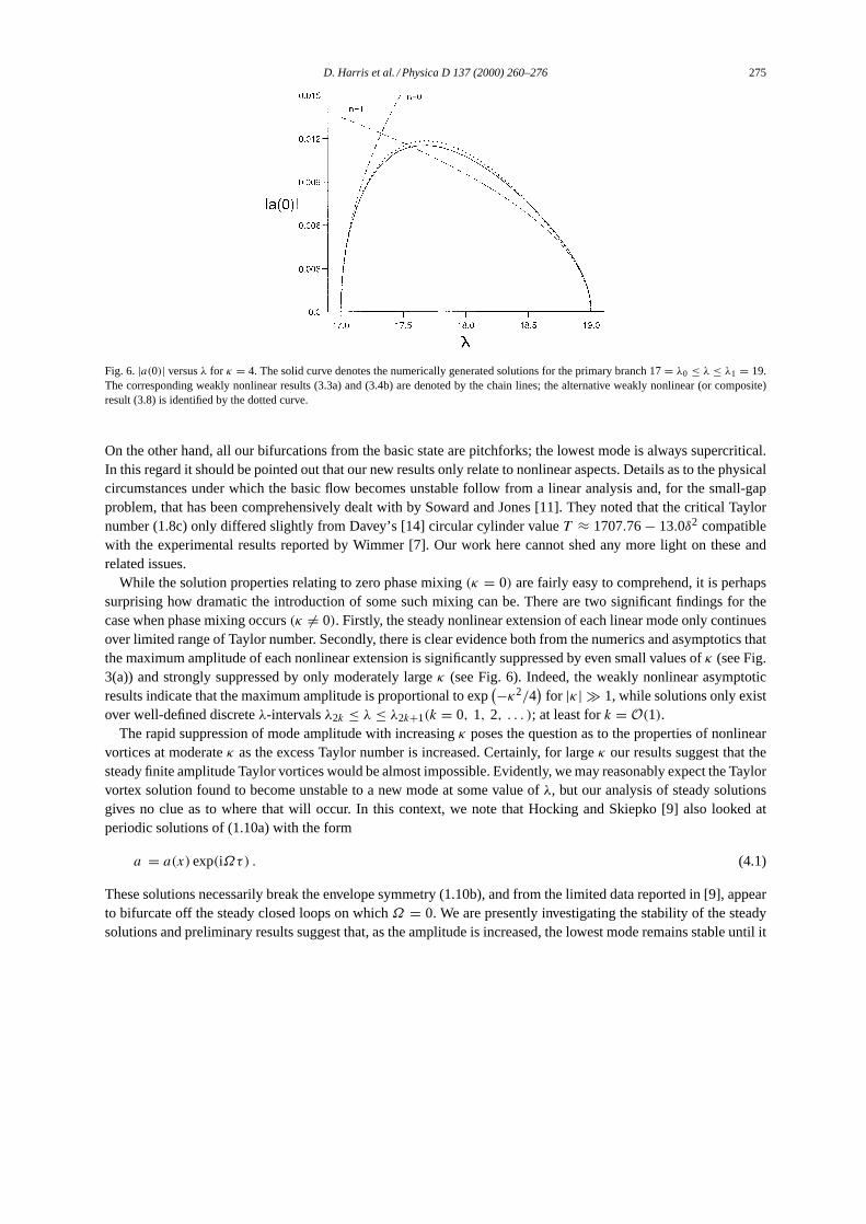
At the low values ofκ used in Fig. 3 both the zeroth and first linearised modes are supercritical. Not only is thisbehaviour clear from these figures but we observe how nonlinear solutions exist over a large, but finite, range ofλ.In Fig. 6 we illustrate the changes that occur at largerκ (hereκ = 4). We continue to restrict attention to the firstlobe of Fig. 3, for which the linear solutions are located on theλ-axis atλ0 = 1+ κ2 = 17 andλ1 = 3+ κ2 = 19.Though our weakly nonlinear results (3.3) and (3.4) show that the former remains supercritical in nature, the result(3.4b) predicts that the latter is now subcritical. This is exactly what is seen from the full nonlinear computations,and moreover, there are two further significant modifications from the small-κ findings of Figs. 3 and 4. First,our solutions only exist forλ0 ≤ λ ≤ λ1, and second, we note how the maximum mode amplitude is stronglysuppressed. On Fig. 6 we have taken the opportunity to superimpose the weakly nonlinear results (3.3b) and (3.4b)of Section 3.1 relating to the leading even and odd modes. Though these simple results provide good approximationsto a large portion of the numerically determined fully nonlinear curve, it is even more striking how the|κ| 1composite approximation (3.8) compares extremely favourably over the entire range.

4. Discussion

We have concerned ourselves here with a study of a steady nonlinear amplitude equation. It provides a convenientmodel for the behaviour of nonlinear Taylor vortices in a narrow gap between two concentric spheres with a commonaxis of rotation. Interestingly, the two parameters in our Eq. (1.10a) admit simple physical interpretation in termsof the phase mixing element and the elevation of the Taylor number above its local neutral value.

We have already recorded that there is extensive experimental evidence that the transitions in spherical Couetteflow can be very complicated and our results derived here lend further credence to this view. That is not to say thatevery aspect of transition is involved in our model. For example, it is the well documented fact (see the experimentalpapers cited earlier) that the basic flow undergoes a pitchfork bifurcation to an eigenmode that is antisymmetric inθ

at a transition Reynolds number that is known for several gap ratios. In view of the WKBJ ansatz (1.5) our analysiscannot distinguish between modes that are symmetric and antisymmetric about the equator. This is because there area very large number of equatorial vortices in the smallε limit and the precise location of the cell boundaries relativeto the equator is a high order effect which our lower order theory is unable to capture. Though our analysis hasdiscussed the symmetry of the large scale envelope, that may be different to the symmetry of the small scale flow.


Fig. 6.|a(0)| versusλ for κ = 4. The solid curve denotes the numerically generated solutions for the primary branch 17= λ0 ≤ λ ≤ λ1 = 19.The corresponding weakly nonlinear results (3.3a) and (3.4b) are denoted by the chain lines; the alternative weakly nonlinear (or composite)result (3.8) is identified by the dotted curve.

On the other hand, all our bifurcations from the basic state are pitchforks; the lowest mode is always supercritical.In this regard it should be pointed out that our new results only relate to nonlinear aspects. Details as to the physicalcircumstances under which the basic flow becomes unstable follow from a linear analysis and, for the small-gapproblem, that has been comprehensively dealt with by Soward and Jones [11]. They noted that the critical Taylornumber (1.8c) only differed slightly from Davey’s [14] circular cylinder valueT ≈ 1707.76− 13.0δ2 compatiblewith the experimental results reported by Wimmer [7]. Our work here cannot shed any more light on these andrelated issues.

While the solution properties relating to zero phase mixing(κ = 0) are fairly easy to comprehend, it is perhapssurprising how dramatic the introduction of some such mixing can be. There are two significant findings for thecase when phase mixing occurs(κ 6= 0). Firstly, the steady nonlinear extension of each linear mode only continuesover limited range of Taylor number. Secondly, there is clear evidence both from the numerics and asymptotics thatthe maximum amplitude of each nonlinear extension is significantly suppressed by even small values ofκ (see Fig.3(a)) and strongly suppressed by only moderately largeκ (see Fig. 6). Indeed, the weakly nonlinear asymptoticresults indicate that the maximum amplitude is proportional to exp

(−κ2/4)

for |κ| 1, while solutions only existover well-defined discreteλ-intervalsλ2k ≤ λ ≤ λ2k+1(k = 0, 1, 2, . . . ); at least fork = O(1).

The rapid suppression of mode amplitude with increasingκ poses the question as to the properties of nonlinearvortices at moderateκ as the excess Taylor number is increased. Certainly, for largeκ our results suggest that thesteady finite amplitude Taylor vortices would be almost impossible. Evidently, we may reasonably expect the Taylorvortex solution found to become unstable to a new mode at some value ofλ, but our analysis of steady solutionsgives no clue as to where that will occur. In this context, we note that Hocking and Skiepko [9] also looked atperiodic solutions of (1.10a) with the form

a = a(x) exp(iΩτ) . (4.1)

These solutions necessarily break the envelope symmetry (1.10b), and from the limited data reported in [9], appearto bifurcate off the steady closed loops on whichΩ = 0. We are presently investigating the stability of the steadysolutions and preliminary results suggest that, as the amplitude is increased, the lowest mode remains stable until it


attains its largest amplitude. The subsequent time development following the bifurcation is revealing some curiousfeatures, whose resolution is the objective of ongoing studies. This should provide further information as to thecomplex nature of the bifurcations which can occur in the nonlinear regime of what is a conceptually simple yetpractically important system (1.10a).

Finally we stress that the asymptotic validity of our results for the narrow gap, almost co-rotation limit (1.9) isquite extreme. They certainly cannot be expected to capture features that are special to the medium or large gapregimes. Indeed, although the linear results appear to agree well with experiment in the narrow gap regime, weare unaware of any experiments that can be reasonably compared with our nonlinear results. This is probably dueto the nature of our approximations, whose implementation depends on the presence of a large number of Taylorvortices. Few experiments seem to have focussed attention on gaps which are sufficiently narrow to sustain manyvortices. We may therefore speculate that our nonlinear results pertain to a fourthverynarrow gap regime and itwould certainly be of considerable interest if future numerical or experimental results confirmed its existence.

Acknowledgements

We thank Leslie Hocking for helpful discussions and the referees for many useful comments which helped toimprove the presentation of this work. The work of DH was supported by an EPSRC studentship which is gratefullyacknowledged. This study was completed while AB was at the School of Mathematics, University of New SouthWales. He is grateful to the Royal Society and the Australian Research Council whose grants made this visit possible.Further thanks are due to the staff of the School (especially Peter Blennerhassett) and to the staff and students ofNew College UNSW for their hospitality.

References

[1] P.S. Marcus, L.S. Tuckerman, Simulation of flow between concentric rotating spheres 1. Steady states, J. Fluid Mech. 185 (1987) 1–30.[2] P.S. Marcus, L.S. Tuckerman, Simulation of flow between concentric rotating spheres 2. Transitions, J. Fluid Mech. 185 (1987) 31–65.[3] K. Bühler, Symmetric and asymmetric Taylor vortex flow in spherical gaps, Acta Mech. 81 (1990) 3–38.[4] M. Liu, C. Blohm, C. Egbers, P. Wulf, H.J. Rath, Taylor vortices in wide spherical shells, Phys. Rev. Lett. 77 (1996) 286–289.[5] C.K. Mamum, L.S. Tuckerman, Asymmetry and Hopf bifurcation in spherical Couette flow, Phys. Fluids 7 (1995) 80–91.[6] M. Wimmer, Experiments on a viscous flow between concentric rotating spheres, J. Fluid Mech. 78 (1976) 317–335.[7] M. Wimmer, Experiments on the stability of viscous flow between two concentric rotating spheres, J. Fluid Mech. 103 (1981) 117–131.[8] I.C. Walton, The linear stability of the flow in the narrow spherical annulus, J. Fluid Mech. 86 (1978) 673–693.[9] L.M. Hocking, J. Skiepko, The instability of flow in the gap between two prolate spheroids. Part I. Small axis ratio, Quart. J. Mech. Appl.

Math. 34 (1981) 57–68.[10] L.M. Hocking, The instability of flow in the narrow gap between two prolate spheroids. Part II. Arbitrary axis ratio, Quart. J. Mech. Appl.

Math. 34 (1981) 475–488.[11] A.M. Soward, C.A. Jones, The linear stability of the flow in the narrow gap between two concentric rotating spheres, Quart. J. Mech. Appl.

Math. 36 (1983) 19–41.[12] J. Heyvaerts, E.R. Priest, Coronal heating by phase-mixed shear Alfvén waves, Astronomy & Astrophysics 117 (1983) 220–234.[13] P. Huerre, P.A. Monkewitz, Local and global instabilities in spatially developing flows, Ann. Rev. Fluid Mech. 22 (1990) 473–537.[14] A. Davey, The growth of Taylor vortices in flow between rotating cylinders, J. Fluid Mech. 14 (1962) 336–368.[15] E.L. Koschmieder, Bénard Cells and Taylor Vortices, Cambridge Monographs on Mechanics and Applied Mathematics, Cambridge

University Press, Cambridge, 1993.[16] M. Abramowitz, I.A. Stegun, A handbook of mathematical functions, National Bureau of Standards, Frankfurt, 1965.[17] S.P. Hastings, J.B. McLeod, A boundary value problem associated with the second Painlevé transcendent and the Korteweg–de Vries

equation, Arch. Rat. Mech. Anal. 73 (1980) 31–51.

an inhomogeneous landau equation with application to spherical couette flow in the narrow gap limit

Documents