an interactive visualization tool for mobile objects
TRANSCRIPT

AN INTERACTIVE VISUALIZATION TOOL FOR MOBILE OBJECTS
by
Tetsuo Kobayashi
A dissertation submitted to the faculty of The University of Utah
in partial fulfillment of the requirements for the degree of
Doctor of Philosophy
Department of Geography
The University of Utah
May 2011

Copyright Ⓒ Tetsuo Kobayashi 2011
All Rights Reserved

T h e U n i v e r s i t y o f U t a h G r a d u a t e S c h o o l
STATEMENT OF DISSERTATION APPROVAL
The dissertation of
has been approved by the following supervisory committee members:
, Chair Date Approved
, Member Date Approved
, Member Date Approved
, Member Date Approved
, Member Date Approved
and by , Chair of
the Department of
and by Charles A. Wight, Dean of The Graduate School.
Tetsuo Kobayashi
Harvey J. Miller 07/07/2010
George F. Hepner 10/25/2010
Olivia R. Liu Sheng 07/07/2010
Ikuho Yamada 07/07/2010
Atsuyuki Okabe
Harvey J. Miller
Geography
ABSTRACT
Recent advancements in mobile devices – such as Global Positioning System
(GPS), cellular phones, car navigation system, and radio-frequency identification (RFID)
– have greatly influenced the nature and volume of data about individual-based
movement in space and time. Due to the prevalence of mobile devices, vast amounts of
mobile objects data are being produced and stored in databases, overwhelming the
capacity of traditional spatial analytical methods.
There is a growing need for discovering unexpected patterns, trends, and
relationships that are hidden in the massive mobile objects data. Geographic
visualization (GVis) and knowledge discovery in databases (KDD) are two major
research fields that are associated with knowledge discovery and construction. Their
major research challenges are the integration of GVis and KDD, enhancing the ability to
handle large volume mobile objects data, and high interactivity between the computer
and users of GVis and KDD tools.
This dissertation proposes a visualization toolkit to enable highly interactive
visual data exploration for mobile objects datasets. Vector algebraic representation and
online analytical processing (OLAP) are utilized for managing and querying the mobile
object data to accomplish high interactivity of the visualization tool. In addition,
reconstructing trajectories at user-defined levels of temporal granularity with time
aggregation methods allows exploration of the individual objects at different levels of

iv
movement generality. At a given level of generality, individual paths can be combined
into synthetic summary paths based on three similarity measures, namely, locational
similarity, directional similarity, and geometric similarity functions. A visualization
toolkit based on the space-time cube concept exploits these functionalities to create a
user-interactive environment for exploring mobile objects data. Furthermore, the
characteristics of visualized trajectories are exported to be utilized for data mining, which
leads to the integration of GVis and KDD.
Case studies using three movement datasets (personal travel data survey in
Lexington, Kentucky, wild chicken movement data in Thailand, and self-tracking data in
Utah) demonstrate the potential of the system to extract meaningful patterns from the
otherwise difficult to comprehend collections of space-time trajectories.

TABLE OF CONTENTS
ABSTRACT. ...................................................................................................................... iii
LIST OF FIGURES. ......................................................................................................... vii
LIST OF TABLES. ............................................................................................................ ix
ACKNOWLEDGEMENTS. ............................................................................................... x
1 INTRODUCTION. ...................................................................................................... 1
1.1. Background. ......................................................................................................... 1 1.2. Research Objectives. ............................................................................................ 7 1.3. Structure of This Dissertation. .............................................................................. 9
2 LITERATURE REVIEW . ........................................................................................ 11
2.1. Time Geography . ............................................................................................... 11 2.2. Knowledge Discovery in Databases and Geovisualization . .............................. 13 2.3. Activity-based Analysis. .................................................................................... 33 2.4. Summary. ........................................................................................................... 37
3 METHODOLOGY. ................................................................................................... 41
3.1. Overview. ........................................................................................................... 41 3.2. Vector Algebra. .................................................................................................. 43 3.3. Aggregation Methods. ........................................................................................ 44 3.4. Data Summarization. .......................................................................................... 58 3.5. Data Exploration Process. .................................................................................. 60 3.6. Summary. ........................................................................................................... 63
4 DATA. ....................................................................................................................... 74
4.1. Overview. ........................................................................................................... 74 4.2. Personal Travel Data Survey in Lexington, Kentucky. ...................................... 74 4.3. Wild Chicken Movement Data in Thailand. ...................................................... 75 4.4. Self-tracking Data in Utah. ................................................................................. 77 4.4. Summary. ........................................................................................................... 78
5 RESULTS. ................................................................................................................. 79

vi
5.1. Overview. ........................................................................................................... 79 5.2. Aggregation Methods. ........................................................................................ 79 5.3. Data Summarization. .......................................................................................... 87 5.4. Summary. ........................................................................................................... 92
6 DISCUSSION AND CONCLUSION. .................................................................... 114
6.1. Summary. ......................................................................................................... 114 6.2. Contributions. ................................................................................................... 115 6.3. Future Research Development. ......................................................................... 116 6.4. Conclusion. ....................................................................................................... 120
LITERATURE CITED. .................................................................................................. 122
LIST OF FIGURES
Figure Page
2.1: Space-time path. ........................................................................................................ 38
2.2: Space-time prism. ...................................................................................................... 38
2.3: A general space-time prism ........................................................................................ 39
2.4: Space-time cube. ........................................................................................................ 39
3.1: An example of visualized vectors in two-dimensional space. ................................... 64
3.2: Time range and time interval. .................................................................................... 64
3.3: Locational similarity. ................................................................................................. 65
3.4: An example of locational vector aggregation. ........................................................... 65
3.5: Locational aggregation ............................................................................................. 66
3.6: Directional statistics and classification of trajectories as vectors. ............................. 66
3.7: Calculation of egocentric direction. ........................................................................... 67
3.8: An example of a space-time path as a point using three indices................................ 67
3.9: Example of geometric vector classification. .............................................................. 68
3.10: Locality. ................................................................................................................... 68
3.11: Convex hull of paths. ............................................................................................... 69
3.12: Spatial range. ........................................................................................................... 69
3.13: Core objects. ............................................................................................................ 70
3.14: Density-reachability and density-connectivity. ....................................................... 71

viii
3.15: DBSCAN in this research ........................................................................................ 72
3.16: Axis conversion. ...................................................................................................... 73
5.1: Visualization with three different time ranges. .......................................................... 93
5.2: Visualization with three different time intervals. ....................................................... 93
5.3: Visualization of Lexington data with different time intervals. .................................. 94
5.4: Time ranges and locational similarity. ....................................................................... 95
5.5: Oversimplification with locational similarity. ........................................................... 96
5.6: Locational similarity and time ranges across different dates. .................................... 96
5.7: Locational similarity with self-tracking data within 1 day. ....................................... 97
5.8: Comparison of movement at the same period in 2 different years. ........................... 97
5.9: Locational similarity and time range within 1 day. ................................................... 98
5.10: Locational similarity and self-tracking movement in the morning time period. ..... 99
5.11: Temporal granularity and locational similarity. ..................................................... 100
5.12: Egocentric directional similarity and time ranges across different dates .............. 101
5.13: Egocentric directional similarity and time ranges in the morning across different dates. ................................................................................................................. 102
5.14: Egocentric directional similarity and time ranges in the morning within
1 day. ................................................................................................................. 103 5.15: Time range and geometric similarity. .................................................................... 104
5.16: Geometric similarity and Lexington data. ............................................................. 105
5.17: Geometric similarity and three different time ranges within a day. ...................... 105
5.18: Axis conversion and geometric similarity. ............................................................ 106
5.19: Statistical information. ........................................................................................... 107
5.20: Outlier detection and refined visualization. ........................................................... 107
5.21: Number of clusters detected with statistical information. ..................................... 108

LIST OF TABLES
Table Page
2.1: Characteristics of activity-based analysis and conventional model process.............. 40
5.1: Result of decision tree of wild chicken data with various time ranges . .................. 109
5.2: Result of decision tree of self-tracking data with various time ranges . ................... 110
5.3: Result of decision tree of Lexington data with various time ranges . ....................... 111
5.4: Decision tree analysis of wild chicken data with time interval and geometric similarity threshold . .......................................................................................... 112
5.5: Decision tree analysis of self-tracking data with time intervals. .............................. 113
5.6: Decision tree analysis of Lexington data with various geometric similarity thresholds. .......................................................................................................... 113

ACKNOWLEDGEMENTS
This dissertation would not have been achievable without the guidance and
support of my committee: Dr. Harvey Miller (Chair), Dr. George Hepner, Dr. Atsuyuki
Okabe, Dr. Olivia Sheng, and Dr. Ikuho Yamada. Thank you for always encouraging me
and providing invaluable feedback every step of the way.
I would like to thank Mr. Toshiaki Satoh and Mr. Tetsutaro Mameda for
countless support in programming skills from basic coding process to advanced 3D
visualization modeling. Also, I would like to thank Mr. Andrei Ostanin for discussions
and training for C# programming with Visual Studio 2008.
Many people supported me in the data collection process. I would like to thank
Dr. Atsuyuki Okabe for providing the precious wild chicken datasets from Thailand. The
DIGIT lab and Scott Bridwell worked hard to refine the Lexington mobility data and
provided the data that fulfilled my request.
Finally, I would like to thank my parents and family for supporting me in every
aspect of my dissertation work and for their encouragement along the way.
1 INTRODUCTION
1.1 Background
Recent advancements in mobile devices –– such as Global Positioning System
(GPS), cellular phones, car navigation system, and radio-frequency identification (RFID)
–– have greatly influenced the nature and volume of data about individual-based
movement in space and time (Golledge & Stimson, 1997). These mobile devices are
used in various applications: navigation systems that support the best route choice for
vehicles; wayfinding to support navigation; real-time tracking of individuals, vehicles,
animals, and other mobile objects; emergency management as responses to accidents,
interruptions of essential services, and disasters (Brimicombe & Li, 2006). This
infrastructure provided by mobile devices, generally called Location-Based Services
(LBS), is changing the lifestyles of people in urban areas dramatically (Li & Longley,
2006).
Individual-based information acquired by LBS is often utilized within
applications of Geographic Information Science (GISci). LBS are defined as the delivery
of data and information services where the content of those services is customized to the
current or some projected location and context of the user (Brimicombe & Li, 2006).
They attract the attention of the GISci community because of their potential to provide
the basis of location-aware information. Location-aware information enables individuals
on the move to communicate with others using wireless mobile devices, and user-
solicited information –– real-time information such as weather forecast, traffic conditions,
2
and maps (Brimicombe & Li, 2006). Although LBS have just started to be developed,
much research has been done to cultivate and strengthen their implementability and
demand (Laurini, Servigne, & Tanzi, 2001; Leonhardt, Magee, & Dias, 1996; Sage 2001).
For example, some research proposes a tourism information system to support the
decision making of tourists (Mountain & Raper, 2001; Zipf, 2002) while others focus on
the user’s needs of location-aware services (Kaasinen, 2003). Moreover, RFID tags can
track patients in hospitals to enhance the operational efficiency of a health delivery
network (Sangwan, 2005). These applications generate locational information with
respect to time for individuals in vehicles or objects with location recording devices.
These individual-based spatio-temporal data are often called mobile objects data (MOD).
MOD have a more complicated structure than traditional spatial data. As stated
above, what is common to all LBS is time-stamped locational data. In other words, the
user of mobile devices can record their locations across time as digital information stored
in databases for future use. In GIS, an object is represented as a point that is moving
through space according to time. Thus, the movement of an object is represented as a
trajectory within three-dimensional space – two spatial dimensions and one time
dimension (Pfoser 2002).
Since mobile objects can change their locations continuously through time, dynamic
representation of entities is required to handle the time component of MOD. However,
most current GISci theories are based on a static place-based standpoint, or static
approach, and thus, they are not well-suited in providing tools for incorporating the time
dimension of geographic information (Mark 2003). Although many efforts have been
made to incorporate a time component in GIS (Peuquet & Duan, 1995; Yuan, 1999),
3
those methods are not adapted to analyze the dynamics of activity and travel behavior of
disaggregate data, or MOD (Wang & Cheng, 2001).
Because of their unique characteristics, the change from static-approach to
dynamic-approach data representation brings many research challenges for MOD: high
data volume, complex data relationships, and nonstandard data query and data analysis
requirements (Shaw & Wang, 2000). Individual-based data is very detailed and therefore,
the data volume can be large. Due to the prevalence of mobile devices, vast amounts of
MOD are being produced and stored in databases (Mountain, 2005). Tools and
applications in current GISci are not designed with the needed capacity to handle the
large volume data associated with MOD (Wang & Cheng, 2001). Second, individual-
based data can have complex relationships among entities. For example, each mobile
object has its own trips and anchors but the movement or trip can be interrelated with
other mobile objects. This complex relationship among mobile objects must be
represented or computed. Third, to represent the complex relationships among the
entities in individual-based data, a new database design is required for data query and
data analysis of mobile objects (Wolfson, Xu, Chamberlain, & Jiang, 1998).
In addition to the research challenges stated above, there is an urgent need to
develop analytical methods for MOD in GISci. Traditional spatial analytical methods
were developed when data collection was difficult and computational power was low
(Miller, 2009). Traditional statistical methods such as spatial statistics, for example,
require high computational loads. Therefore, traditional methods that are based on small
volumes of information are not applicable for large volume and diverse geographic
information, including MOD. Moreover, traditional spatial analytical methods are

4
confirmatory and the researchers need to have an a priori hypotheses. Therefore,
traditional spatial analytical methods cannot discover unexpected patterns, trends, or
relationships that are embedded in large volume spatio-temporal data such as MOD. A
major challenge is to develop appropriate models and techniques to manage, analyze, and
visualize such large datasets to extract meaningful patterns, trends, and relationships
(Frihida, Marceau, & Theriault, 2004).
Conceptual and technological frameworks have been developed to address useful
patterns and relationship within large, multivariate spatio-temporal data including MOD
(Frihida et al., 2004). These are referred to as Geovisualization (GVis) and Knowledge
Discovery in Databases (KDD): they are two major research fields that are associated
with knowledge discovery and construction. Although their approaches to knowledge
discovery are different from each other, their primary goal is to find, relate, and interpret
interesting, meaningful, and unanticipated features (objects or patterns) in large data sets
(MacEachren, Wachowicz, Edsall, & Haug, 1999). The difference is that GVis relies
upon human vision whereas KDD is based on computational methods. In addition,
methods of GVis and KDD both require interactivity to be effective (MacEachren et al.,
1999). Neither a single visual exploration nor a single data mining run is helpful to find
the interesting, unexpected knowledge embedded in data – repeated application of the
methods are required.
There are several research challenges in GVis and KDD to handle spatio-temporal
datasets such as MOD. One of the major research challenges is the integration of GVis
and KDD: much KDD research emphasizes the importance of visualization, although
GVis is mostly used as a technique to interpret and evaluate the results of analysis in

5
KDD (MacEachren et al., 1999). Another research challenge is to incorporate large
volume spatio-temporal datasets into GVis tools. Although KDD tools are designed for
large volume datasets, many GVis tools are not applicable for large datasets. Efficient
GVis tools that can handle massive volumes of spatio-temporal data are required. In
addition, interaction between human and machine is also a research challenge in GVis
and KDD –– high interactivity of GVis tools is necessary to accomplish better intuitive
knowledge discovery.
There have been many efforts in GVis and KDD research to solve the problems
stated above. Some studies enhanced the interactivity of visualization tools by extracting
features that characterize the mobile objects such as direction and velocity (Laube, Imfeld,
& Weibel, 2005; Mountain, 2005; Smyth, 2001). Other research proposed new methods
of representation and visualization of mobile objects (Imfeld, 2000; Laube et al., 2005).
Moreover, data mining methods were incorporated in visualization tools for further data
exploration (Dykes & Mountain, 2003; Mountain, 2005). This research expanded the
capability of GISci to be applicable to handle spatio-temporal data, including MOD.
In addition to the grand challenges in GVis and KDD for spatio-temporal datasets,
some research problems describing the movement of mobile objects have been proposed
(Laube et al., 2005). They are as follows:
• Uncertain and missing data
• Interpolation issues
• Analysis granularity for time component
• Aggregation of mobile objects
• Factors or characteristics of the motion attributes.

6
First, there are usually uncertain and missing data in real-world tracking data.
However, existing methods are designed for complete data that are without uncertain or
missing portions, and methods to deal with those incomplete data should be developed.
Second, to solve the problem of uncertain and missing data, interpolation methods for
missing tracking points of mobile objects are needed (Wentz, Campbell, & Houston,
2003). Third, the sampling rate in time for the mobile objects should be the same so that
the analysis will be performed with the data of the same time granularity. Since MOD
collected by different devices may have different time sampling rates, compatibility
between data from different data collection process should be discussed and solved to
incorporate and analyze the data from various data sources. Fourth, similar to the spatial
scale problem known as Modifiable Areal Unit Problem (MAUP), the time scale should
also be considered in the analysis of MOD (Hornsby, 2001). If MOD are explored in
different time granularity with the interactive visualization tools, different patterns or
relationships can be detected from the data exploration. Therefore, aggregation methods
for the time component should be developed. Fifth, more factors or characteristics of the
mobile objects can be added to interactive data exploration. Previous works show that
only a few characteristics – such as direction, speed, or velocity – are available to the
user of the visualization tools to explore the data. There can be more characteristics or
attributes of the trajectories of mobile objects and those factors should be added to the
visualization tools. It is not only that these five challenges still remain unsolved, but also
that there is no standard method to deal with the problems. Although the interactive
visualization tool must be data-driven or task-driven (Andrienko, Andrienko, & Gatalsky,

7
2005), these challenges are the tasks that can be applied to any kinds of MOD – a more
integrated visualization tool that overcomes these three problems should be developed.
1.2 Research Objectives
This dissertation proposes methods to uncover patterns, trends, and relationships
that are hidden in massive volumes of MOD data. Emergence of MOD data enables us to
develop geographic theories from a people-based perspective instead of a place-based
approach, which is basically a collection of functions of locations and was the
mainstream when data were scarce and computational platforms were weak (Miller,
2005a).
A people-based perspective focuses on individual-based (or disaggregate) activity
patterns and accessibility in space and time (Miller, 2005b). The mobility of individuals
has increased due to the development of advanced transportation systems and settlement
systems. In addition, telecommunication systems, The World Wide Web, and related
internet technologies, including location-aware technologies and social medias, have
been altering the nature of allocating space and time in people’s daily lives. As Miller
(2005a) states;
the world is shrinking in an absolute sense: transportation and communication costs have collapsed to an incredible degree over the last two centuries (Janelle, 1969). The world is also shriveling as relative differences in transportation and telecommunications costs are increasing at most geographic scales (Tobler, 1999). The world is also fragmenting: people and activities are becoming disconnected from location (Couclelis & Getis, 2000). (p. 216)
A place-based approach is not well-suited in the era of massive mobility information that
contains dynamic spatial, temporal, and attribute information of individuals.

8
As stated previously in this chapter, there is an urgent need to develop methods
that can handle massive volumes of disaggregate level mobility data. Since there is no
standard a priori knowledge about the nature of individual mobility information
established yet, exploratory analysis rather than confirmatory analysis is appropriate to
discover underlying patterns. Therefore, exploratory spatial data analysis such as data
visualization and data mining plays a key role in this phase.
This dissertation proposes a visualization toolkit as a means of exploratory visual
and quantitative analysis for MOD data, which leads to research at a more detailed and
deeper level, such as hypothesis creation of geographic theories, and assessment of
geographic models that have not been discovered or developed. Insights from exploratory
analysis have great potential in transforming MOD data into useful and meaningful
geographic thoughts.
The visualization toolkit in this dissertation also provides GVis tool components
to overcome research problems for MOD, integration of GVis and KDD, handling large
volumes of MOD, enhancement of interactivity of GVis tool, manipulation of time
granularity, and aggregation and summarization of mobile objects. The research
objectives are as follows:
• To create a highly interactive graphical user interface (GUI) for visual data analysis
of mobile objects
• To develop methods to visualize large volume MOD using vector algebra and online
analytical processing (OLAP)

9
• To propose methods for aggregation and summarization of vector algebraic
representation of MOD for better visual data exploration and knowledge discovery
construction.
A highly interactive visualization toolkit enables users to explore the data from
various perspectives. The users manipulate data using spatial, temporal, geometric, and
other geographical components of the data, which is explained in detail in Chapter 3. The
ability to handle large volume data has been one of the major research challenges in
GISci. Moreover, functionalities such as aggregation and summarization of MOD data
enhance the interactivity of the data exploration and provide new insights in visual data
exploration. Also, the integration of GVis and KDD is accomplished by incorporating the
functionality of data mining in the toolkit. The toolkit consists of novel functionalities for
pattern detection in MOD data towards knowledge construction of individual human
activity in space and time.
1.3 Structure of This Dissertation
This dissertation consists of six chapters. Chapter 1 introduces the current
research challenges, proposing goals and objectives of this dissertation. Chapter 2
reviews literature of related research fields that contributed to GISci research for MOD:
time geography, GVis, knowledge discovery in databases, and activity-based analysis.
Since this research focuses on visualization and knowledge discovery, a large portion of
the literature review is dedicated to these two research fields. Chapter 3 describes
techniques that are utilized in the visualization tool and management of MOD: vector
algebra and OLAP. It also proposes the methods for aggregation and summarization of
vector representation of mobile objects; several similarity functions are presented.

10
Chapter 4 describes the MOD that are used in this dissertation: wild chicken data in
Thailand; GPS tracked data of Lexington, Kentucky; and GPS self-tracking data of the
investigator. Chapter 5 presents the results of the visual data exploration and data mining,
evaluating the versatility of the visualization tool to various MOD. Chapter 6 then
summarizes and concludes the dissertation and proposes the future agenda that this
research suggests.
2 LITERATURE REVIEW
2.1. Time Geography
Time geography is the study of individual-based human behavior in space and
time. It was originally introduced to the English-speaking world by Hägerstrand in 1970.
Time geography focuses on constraints on human behavior rather than the prediction of
human spatial behavior. The core notion of time geographic framework is that events
comprising an individual’s existence have both spatial and temporal attributes.
Three constraints limit the ability of individuals to move and participate in
activities: capability constraint, coupling constraint, and authority constraint. Capability
constraint refers to the person’s ability to trade time for space in movement. For example,
the need for food or sleep constrains peoples’ movement because people need such things
for everyday life. Coupling constraint relates to the possibility of two or more persons
interacting. Authority constraint limits the movement of people to certain places or
domains in space and time. For example, people cannot go inside a shopping mall when it
is closed (Hägerstrand, 1970).
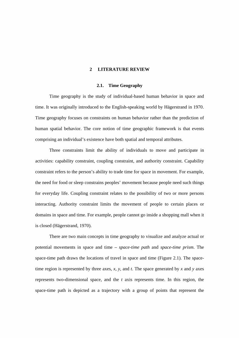
There are two main concepts in time geography to visualize and analyze actual or
potential movements in space and time – space-time path and space-time prism. The
space-time path draws the locations of travel in space and time (Figure 2.1). The space-
time region is represented by three axes, x, y, and t. The space generated by x and y axes
represents two-dimensional space, and the t axis represents time. In this region, the
space-time path is depicted as a trajectory with a group of points that represent the

12
sequence of locations of individual movement in space and time.
In addition to space-time path, the space-time prism provides the possible
movement areas that an individual can access with a limited amount of time. Figure 2.2
illustrates a basic prism without the activity time. The area bounded by the upper cone
and lower cone is called the potential path space (PPS); this represents the area an
individual can travel in space based on leaving the first location at time ti and arriving at
the second location at time tj, traveling at the maximum velocity. Also, the area in two-
dimensional space projected from the PPS is called the potential path area (PPA). Using
these basic time geographic entities, the possibility and limitation of individual
movements can be determined. Figure 2.3 shows a more general case of the space-time
prism. The first activity is at a fixed location xi, which ends at time ti, while the second
activity location is at the fixed location xj, which starts the activity at time tj. The
minimum time required for the individual to participate in the activity is represented as aij.
Since this time geographic concept has been proposed, many efforts have been
conducted to improve the analytical framework of time geography (Miller, 1991, 1999;
Kwan & Hong, 1998). Recently, an analytical definition of time geography has been
proposed to expand the availability of the time geographic concept in geographic
information science (Miller, 2005c). In addition, detailed descriptions of time geographic
concepts, such as error analysis and uncertainty analysis, have been discussed as well
(Hall, 1983; Neutens, Witlox, Van De Weghe, & De Maeyer, 2007). Hornsby and
Egenhofer (2002) developed a framework that enables space-time queries in multiple
time granularity for space-time paths, space-time prisms, and when paths and prisms are
combined.

13
A primary concern of time geography is individual accessibility. This includes
issues such as pattern detection of accessibility in urban areas (Kwan, 1999; Lenntorp,
1976, 1978), coupling possibility (Neutens, Schwanen, & Miller, 2009), and detection of
gender differences in space-time movements (Kwan, 2003). In addition, a desktop
software application of GIS to measure and visualize the PPA was developed to support
the decision making of journeys using a public transportation system (O’Sullivan
Morrison, & Shearer, 2000). Furthermore, the prediction of the travel behavior rising
from cognitive maps was also attempted (Mondschein, Blumenberg, & Taylor, 2005).
These efforts facilitate the development of applications using a time geographic
framework and extend the scope of time geographic research.
This dissertation applies the time geographic framework for the visualization of
space-time paths in a three-dimensional view. Space-time queries with multitemporal
granularity that are similar to Hornsby and Egenhofer (2002) are utilized as time
aggregation methods. Querying and visualizing space-time paths at different time
granularities extends the ability of exploratory pattern detection and knowledge discovery.
This is an important aspect of Knowledge Discovery in Databases (KDD) and
Geovisualization (GVis).
2.2. Knowledge Discovery in Databases and Geovisualization
The volume, scale, and scope of digital geographic datasets are expanding at a
tremendous rate from the advances in technologies and techniques. Due to the
inadequacy of traditional spatial analysis methods for these massive geographic datasets,
it is time to create a new paradigm to handle large volume, highly multivariate datasets
that require high levels of computation power. Exploratory Data Analysis (EDA), KDD,
14
and GVis are the research fields that attempt to provide methods of exploration, analysis,
and representation of a massive amount of data to extract deeply hidden patterns, trends,
and relationships, and perform knowledge discovery. Although those three research fields
have similar objectives, their foci are different from each other.
2.2.1. Exploratory Data Analysis
EDA seeks patterns and relationships in observational data, as well as
explanations for such patterns and relationships. The basis of EDA is the idea that data
analysis is essentially regarded as an interactive circular process where knowledge is
constructed through the association of theory — such as spatial statistics — and
observational data, or raw data (Tukey, 1977). In this sense, EDA sheds new light on
scientific methods that have never been considered. In addition, scientists no longer have
to rely on a priori assumptions about the data: they can generate new hypotheses rather
than testing existing hypotheses with statistics (Wachowicz, 2005). It is an approach that
searches for patterns and relationships in data and generates hypotheses simultaneously
(Yuan, Buttenfield, Gahegan, & Miller, 2004).
The need for EDA is growing as large volume datasets have been generated with
a variety of applications such as marketing, transportation, finance, and medicine
(Gahegan, 2005). In addition, continuous growth of spatio-temporal datasets in their size
and complexity also facilitates the need for improvements in EDA techniques. One of the
trends in scientific research is the development of interactive visualization tools. Some
EDA methods utilize not only statistical analyses but also cartographic maps for data
exploration (Guo, Liao, & Morgan, 2007; Wachowicz, 2005). Gahegan (2005) identified
two reasons why visualization is useful in exploring such large datasets. First, a virtual

15
environment, such as three-dimensional immersive virtual reality, enables observers’
greater access to a large amount of data than figures and tables. Second, the process of
visualization requires many data transformations, such as 3D-scatterplot and parallel
coordinate plot (Gahegan, Takatsuka, Wheeler, & Hardisty, 2002) — these kinds of
transformations fulfill roles such as querying and focusing operators, and facilitating the
process of uncovering hidden patterns and structures in data. Furthermore, leveraging
human vision in addition to computational methods may lead to deeper insight. This is
why GVis is taking a leading role in the data exploration of massive datasets, including
datasets with complex structure such as spatio-temporal data. It is difficult to distinguish
EDA from GVis and KDD, but EDA is more suitable for very rich datasets, where the
dimensionality of attributes is large, but the size of datasets is smaller. On the other hand,
GVis and KDD are developed for large volume datasets (Wachowicz, 2005).
2.2.2. Geovisualization
A knowledge discovery concept that integrates cartography and scientific
visualization is GVis. It focuses on visual explorations and analysis of geographic
information in the knowledge construction process (Kraak & MacEachren, 1999). GVis
relates to researches in many disciplines such as cartography, scientific visualization,
image analysis, information visualization, exploratory data analysis (EDA), and
GIScience (Dykes, MacEachren, & Kraak, 2005). In addition, GVis tools allow the user
to interact with spatial datasets to seek interesting patterns and structures that are
embedded in the datasets to support the construction process of refined knowledge. It is
also useful as a communication tool in a group for discussions and decision-making
processes.

16
The Commission on Visualization and Virtual Environments of the International
Cartographic Association (ICA) has proposed challenges in GVis and announced
recommendations for actions. According to Dykes et al. (2005), there are four major
research challenges in GVis, namely, representation, visualization-computation
integration, interface design, and cognition-usability.
Representation is a core theme in GVis. The challenge is to develop new forms of
geographic representation based on the new technological advances in both hardware and
data formats. Many geographic representation methods for GVis have been proposed,
including interpolation methods such as triangular irregular network (TIN) and
geostatistical interpolation methods, including kriging (DiBiase, 1990), cartographic
animation (Lobben, 2003), spatialization (Skupin & Fabrikant, 2003), interactive color
arrangements (Brewer, 1997), self-organizing maps for geographic information (Skupin
& Hagelman, 2005; Yan & Thill, 2007), and virtual environments (Dykes, Moore, &
Wood, 1999). Spatio-temporal data collected by emerging devices such as GPS and other
remote sensors can be visualized to analyze spatiotemporal human movements (Laube,
Imfeld, & Weibel, 2005; Mountain, 2005).
Interactions among many variables in large datasets are so complex that purely
visual data exploration by human vision cannot be successful. The aim of visualization-
computation integration is to develop knowledge construction tools through visual data
exploration that enhance the user’s ability to discovering hidden patterns, trends, and
relationships in complex geographic data, and explaining the results of data exploration.
Integration of KDD and GVis to support visual data exploration by processing and
analyzing datasets before visualization is one of the challenges in this integration

17
research agenda. This effort is often accomplished and implemented through the interface
design for GVis.
Development and improvement of GVis interface design is requisite to facilitate
the use of hands-on GVis tools by the public, providing better opportunities for
interactions with large volume geographic data for knowledge discovery. Interface design
ranges from simple color arrangement tools (Brewer, 1997) to complex analysis such as
the combination of visualization and multivariate statistics by GeoVista Studio toolkit
(http://www.geovistastudio.psu.edu/jsp/index.jsp), exploratory data analysis toolkits for
activity/travel data (Buliung & Kanaroglou, 2004) and remotely-sensed data analysis of
individual motions (Laube et al., 2005). Although there are some efforts to create the
interactive properties of GVis with the purpose of creating more understandable tools,
there are few tools that validated the efficiency of visualization methods. Therefore, the
cognition and usability of GVis must be addressed.
The cognitive aspects of GVis focus on human-computer interaction (HCI) such
as perception and reaction of people to the visual representation in GVis tools. Research
with experiments or surveys attempt to explain the human perception of fundamental
geographic notions such as distance, proximity, and scale – these notions are evaluated
for testing cognitive aspects of visualization (Fabrikant, 2001; Fabrikant, Montello,
Ruocco, & Middleton, 2004; Montello & Fabrikant, 2003). In addition, experiments and
surveys are often conducted to evaluate the usability of GVis tools (Dêmsar, 2007;
Fuhrman et al., 2005; Lobben, 2008).
18
2.2.2.1. Research Challenges in GVis
Although GVis has great potential to contribute to knowledge discovery and
construction, GVis research has just begun and there are still many research challenges.
The ICA research agenda provides four “GVis research challenges” (MacEachren &
Kraak, 2001). The next four sections explain those research challenges.
2.2.2.1.1. Experimental and multimodal “maps.” Emerging technologies such
as Virtual Reality reflect the demands of experiential and multisensory interaction (Dykes
et al., 2005). Development of GVis technologies for these modes of information access is
one of the research challenges. There is a general assumption in current GVis research
that the abstraction, summarization, or aggregation of information is essential to discover
meaningful knowledge, while virtual reality explores a more experiential representation
of information for knowledge discovery. Developing technologies that can utilize the
potential of virtual realism and multisensory representation is important for GVis
research in order to incorporate the power to visualize and analyze geographic
information in a more realistic view (Wood, Kirschenbauer, Döllner, Lopes, & Bodum,
2005). Practical applications for immersive environments are navigation systems with
mobile devices (Coors, Elting, Kray, & Laakso, 2005), and training of fieldworkers
(Dykes et al., 1999). Data representation of geographic data and spatio-temporal data
requires powerful rendering techniques due to the size and complexity of those datasets.
Therefore, the capability of handling large datasets is another research challenge.
2.2.2.1.2. Large datasets. Large volume, complex geographic data demands new
techniques, tools, and approaches for better knowledge discovery with GVis. Although
the concept of GVis is to draw upon human visual ability to discover patterns, trends, and
19
relationships from complex data, existing GVis tools are not applicable to large volume
datasets. A key issue here is the development and integration of GVis methods with
geocomputational techniques (discussed later in this chapter) (Gahegan, Wachowicz,
Harrower, & Rhyne, 2001). Since data exploration of complex datasets, such as spatio-
temporal datasets or mobile object data (MOD), requires exploratory functionality from
many perspectives, visualization methods combined with geocomputational methods,
including self-organizing maps and neural networks, have been proposed (Guo, Gahegan,
MacEachren, & Zhou, 2005).
2.2.2.1.3. Group work. Multiuser systems have become more available due to the
advances of telecommunication technologies, providing more opportunities for group
work. However, GVis research has been driven mostly by individual experts, resulting in
tools and methods for individual use (Dykes et al., 2005). There is a growing demand for
developing techniques to support collaborative GVis for better decision-making in
applications such as the decision making process in a time of emergency or crisis
(MacEachren & Cai, 2006). There are several research challenges in this field
(MacEachren & Brewer, 2004):
• Developing a theoretical understanding of the cognitive and social aspects of both
local and remote collaboration mediated through display objects in a geospatial
context (Fuhrman & Pike, 2005; MacEachren & Cai, 2006)
• Development of approaches to multiuser system interfaces that support, rather than
impede, group work (Gahegan et al., 2001; MacEachren, 2005)
• Understanding ways in which the characteristics of methods and tools provided to
support collaboration influence the outcome of group work (Hopfer & MacEachren,

20
2007)
• Initiation of a concerted effort focused on integrating, implementing, and
investigating the role of the visual, geospatial display in collaborative science,
education, design, and group decision support (Brodlie, 2005).
As stated above, works with multidisciplinary efforts are important aspects to
achieve these goals. In addition, it is important to develop and evaluate human-centered
tools and methods for collaborative works that enhance effective human-computer
interaction for better decision making.
2.2.2.1.4. Human-centered approach. Another significant challenge is the
incorporation of human-centered approaches to GVis methods and tools, which leads to
the integration of technological advances of GVis and efforts in human spatial cognition
and the potential of visual representations to enable thinking, learning, problem solving
and decision making (Fabrikant & Skupin, 2005). This is a field that is closely related to
information visualization, whose goals is to provide compact graphical presentations and
user interfaces for interactively manipulating large numbers of items, possibly extracted
from far larger datasets. Plaisant (2005) proposed research challenges towards universal
usability of information visualization tools:
• Development of tools that can handle large volume datasets
• Development of tools that are accessible to a wider group of diverse users
From a GVis perspective, Slocum et al. (2001) proposed research challenges in
the context of cognitive usability:
• Development of geospatial virtual environments
• Dynamic representation methods
21
• Metaphors and schemata in interface design
• Difference in individual work and group work
• Collaborative GVis
• Evaluating the effectiveness of GVis methods
GVis research topics are interrelated to each other since some of the challenges
overlap with other research challenges that MacEachren and Kraak (2001) proposed. For
example, research on spatialization has been utilizing the basic notions of geography —
such as distance and scale — to understand the cognitive aspect in visualization
(Fabrikant et al., 2004; Montello & Fabrikant, 2003) as well as the browsing ability of
spatialized large datasets (Fabrikant, 2000). Classification of interactivity types in GVis
and discussion on the benefits of those interactivity types provide insights for better user-
centered tools (Crampton, 2002). To understand the cognitive aspect of GVis tool users,
evaluation of interactivity and visualization methods is important as well (Brewer, 1997;
Dykes, 2005; Fabrikant, 2001; Fuhrman et al., 2005; Lobben, 2008; Tobón, 2005). In
addition, there are needs for the development of both theories and applications for
universal access and usability for geographic data, requiring new approaches and
methods to support personalization of GVis tools for particular users and groups of users
for GVis tasks (Brodlie, 2005; MacEachren & Kraak, 2001).
Although GVis seeks tools and methods to find patterns and trends in data with
visual exploration, computational methods are also useful to evaluate the results or
findings from visual exploration. In the next section, Knowledge Discovery in Databases
(KDD) focuses on computational methods in data exploration, which can complement
GVis methods.

22
2.2.2. Knowledge Discovery in Databases
KDD is a strategy for analyzing large volume datasets that are stored in databases.
It is defined as ‘the non-trivial process of identifying valid, novel, potentially useful, and
ultimately understandable patterns in data’ (Fayyed, 1996). A need of techniques for the
emerging large volume datasets – along with the improvement in information technology
and subsequent development of monitoring techniques — accelerated the development of
KDD (Miller & Han, 2009; Wachowicz, 2005). The purpose of KDD is to seek hidden
information, trends, characteristics, or structure in the data and create knowledge based
on the findings from the search process. KDD was originally developed by several
disciplines such as statistics, machine learning, pattern recognition, numeric search, and
scientific visualization as an approach for exploring massive datasets that are too
complex and difficult for human abilities to handle (Miller & Han, 2009). Although data
mining is the more popular word for knowledge discovery, KDD is a broader process
than data mining.
There are different descriptions of KDD process, including the nine-step process
proposed by Fayyed (1996) as follows:
• Developing an understanding of the application domain, the relevant prior knowledge,
and the goal of the end-user
• Creating a target data set: selecting a data set, or focusing on a subset of variables or
data samples, on which discovery is to be performed
• Data cleaning and preprocessing: operations such as noise or outlier removal,
strategies for handling missing data fields, and so on
• Data reduction and projection: finding useful features to represent the data depending
23
on the goal of the task
• Choosing the data mining task: determination of the goal of KDD such as
classification, regression, clustering, and so on
• Choosing the data mining algorithm(s): choice of method(s) to be used to seek for
patterns and trends in datasets
• Data mining
• Interpreting mined patterns, possible return to any of the steps above
• Consolidating discovered knowledge: incorporating this knowledge into the
performance system, or simply documenting it and reporting it to users.
Although the process above suggests a linear process for KDD, KDD is an
interactive process that often requires iterative tasks; therefore, KDD does not often
follow a linear progression (Fayyad, 1996; MacEachren et al., 1999). The KDD tasks —
such as segmentation, dependency analysis, deviation and outlier analysis, trend detection,
generalization, and so on— are tied to specific methods — classification, clustering,
querying, and so on: see Miller and Han (2009) and MacEachren et al. (1999) for more
detailed descriptions of KDD tasks and methods.
Data warehousing is a system that integrates data from several sources. It
contains large volume datasets that were collected from many different sources and is
often maintained separately from the operational databases (Shekhar, Lu, Tan, Chawla, &
Vatsavai, 2009). The advantage of utilizing a data warehouse is to provide an integrated
system of dispersed heterogeneous databases so that decision makers receive benefits
from decision support tools that can provide aggregated and summarized data (Bédard &

24
Han, 2009). In short, the goal of data warehousing is to extract useful knowledge from
massive and detailed data dispersed in heterogeneous datasets.
Data warehousing technologies provide functionalities to manipulate datasets for
data exploration. One of the common tools for summarization and integration of datasets
is online analytical processing (OLAP). OLAP provides interactive functionality for
multidimensional summarization of data with simple functions such as drill-down, drill-
up, and drill-across that are built into the data warehousing tools so that the user can
explore multidimensional data at arbitrary granularity levels.
The data cube is an effective OLAP method for summarization of highly
multivariate data. The data cube is an operator that allows the user to aggregate the data
with all the dimensions that user needs. Its extension to geographic data is known as the
map cube. A map cube can handle all the geographic components of spatial data such as
raster format, vector format, network component, reference systems, and so on (Shekhar
et al., 2009).
Although most KDD research focus on nonspatial data, advancement of
technology enabled us to collect a large amount of complex and highly multidimensional
geographic data, including spatio-temporal data, which has led to the development of
geographic KDD methods (Andrienko, Andrienko, Fischer, Mues, & Schuck, 2006;
Frihida et al., 2004; Mennis & Peuquet, 2003). In geographic information science (GISci),
data mining and knowledge discovery techniques applied to explore spatial data are often
called Geographic Knowledge Discovery (GKD).
KDD methods for nonspatial data are not directly applicable to geographic
information because of the data’s nature of high dimensionality, inherent spatial

25
dependency and heterogeneity, the complexity of spatio-temporal objects and rules, and
its diverse data types (Miller & Han, 2009). Geographic information usually has high
dimensionality because it has its locational information, which needs at least two
dimensions, as well as high levels of attribute information. Second, spatial dependency
represents the notion that attributes at proximal locations are more closely related to each
other. On the other hand, however, spatial heterogeneity derives from the uniqueness of
geographic locations. These characteristics are usually treated as something cumbersome
in statistical analysis but they are useful information for exploring geographic phenomena.
Third, it is more complex and difficult to handle spatio-temporal objects and relationships
than handling nongeographic objects and relationships. In addition, handling time in
spatial entities is also a complex task (Hornsby & Egenhofer, 2002). Fourth, since digital
geographic datasets are stored in several different formats, such as vector and raster
format, there is the need to create methods to handle different data formats at the same
time for knowledge construction (Golledge, 2002).
Spatial data mining is also a powerful technique to extract trends or
characteristics from large volumes of geographic information. It encompasses the
application of computational tools to seek for hidden characteristics in spatial and
temporal databases (Miller & Han, 2009). In contrast to traditional data mining, spatial
data mining focuses on the spatial aspects of the data such as locational information of
individuals and sometimes the temporal aspects as well. Common spatial data mining
techniques include spatial segmentation, spatial clustering, spatial trend detection,
geographic characterization and generalization, spatial outlier detection, and so on (see
Miller & Han, 2009 for a more detailed description). Studies have also been conducted

26
with activity diary datasets, such as text mining, that contain location, time, the type of
activity, and the duration of activity (Kwan, 2000), and also with GPS-based datasets
used to explore patterns in spatio-temporal human movements (Smyth, 2009). There is
also an effort to discover outliers in the data using distance as the geographic criteria for
detecting outliers in individual trajectory datasets (Ng, 2001).
The space-time cube is an extended approach of the map cube, especially for
disaggregated spatio-temporal data. It defines a graphic environment that allows the
exploration of data from three axes; x and y axis as the representation of geographic
space, and z axis as the time component (Kraak, 2003). Space-time trajectories can be
visualized after necessary data are queried from the databases and processed by the cube
methods (Figure 2.4).
2.2.3. Integration of GVis and KDD
It is clear that both GVis and KDD aim to find, relate, and interpret interesting,
meaningful, and unknown patterns and relationships in complex and large datasets such
as spatio-temporal datasets (Wachowicz, 2005). KDD research often claims the
importance of visualization in the process. On the other hand, computational methods
expand the capability of visual data exploration not only for map making, including
automation, optimization of the workflow, and ability to easily vary design (Buckley &
Hardy, 2007), but also deeper and better knowledge construction.
Gahegan et al. (2001) proposed some research challenges for the integration of
GVis and KDD in terms of data, system, visual techniques, modes of inference, and
collaboration. In those research challenges, The International Cartographic Association
(ICA) focuses on three issues, namely, the geographic properties of data, the construction

27
of knowledge, and visualization. First, designing useful visualization techniques for large
volume and highly multivariate spatial and spatio-temporal data is an ongoing challenge.
Representation of spatial and time components of data should be investigated. Second,
since there is no universal language for geographic representation, better conceptual
structures are required for computationally based geographical models. It is urgent to
specify geographically oriented concepts to identify, and develop, a means of
representing them in current GIS or database schema. A definition of computational and
visualization methods to detect, observe, and communicate follows below. Third, it is
important to create visualization environments that allow the user to interact with tools
that construct meaning. The challenge here is to construct an environment that can
seamlessly address all mining and knowledge construction activities (Gahegan et al.,
2001).
Wachowicz (2005) proposed the GeoInsight approach for the integration of GVis
and KDD — this is based on the framework of MachEachren and Kraak (2001). The
GeoInsight concept defines integration in three levels: conceptual, operational, and
implementational. The goals are as follows:
• the conceptual level for defining the goals of a knowledge construction process;
• the operational level for integrating the methods developed independently in each of
the fields;
• the implementation level for combining a variety of tools within a singular system
environment.
The conceptual level is used to define the goals of a knowledge discovery process.
This is because unclear goals can lead to a choice of inappropriate methods in a

28
knowledge construction process. The goals based on a knowledge discovery process are
related to the answers of the following questions:
• What kind of spatio-temporal data is meant to be explored?
• What particular kinds of outcomes are required from the process?
• Who are the users interested in the knowledge construction process?
The answers determine the kind of knowledge to be constructed and how the
knowledge is constructed as well. In this conceptual level, no decision is made about the
selection of data mining tasks or algorithms, nor about the choice of visual representation
or visualization tools to be used. The main focus is to understand the prior experience and
the goals of a user, and only after this can we define how the knowledge discovery
process will be constructed.
The operational level specifies appropriate methods, and combinations of
methods, for achieving conceptual goals. In the GeoInsight approach, task analysis
(Kirwan & Ainsworth, 1992) is utilized to support the task-method-operation concept.
Tasks are the main stages of a KDD process. Methods define ‘how’ the tasks can be
performed to achieve the conceptual goal. An operation is a statement of ‘what’ is to be
accomplished by structuring a hierarchical or sequential organization of actions. The
main goal of the task-method-operation concept is to facilitate the human-centered
approach and enhance the interactive and intuitive properties in the knowledge discovery
process.
The implementation level deals with selecting the execution of algorithms to
perform the data mining tasks, and also the operations to build effective visual
representations and interactive forms. The main concern is to create an integrated

29
computer environment with the necessary components for data exploration for each user
— the goal here is to integrate different functionalities into a single computer
environment.
The GeoInsight concept aims to develop a more complete integration between
GVis and KDD, facilitating the development of a more flexible, interactive, and human-
centered knowledge construction process for spatio-temporal data. Spatio-temporal data
and MOD are complex in structure and increasing in size, requiring robust methods and
tools for data exploration, which is discussed in the next section.
2.2.4. GVis and KDD with MOD
As stated in the introduction chapter of this dissertation, MOD are increasingly
available due to the development of mobile devices. Many scientists have been proposing
tools and methods for visualizing and analyzing MOD for better knowledge discovery.
However, there are many issues that relate to the nature of MOD, such as data acquisition
and storage methods, representation methods, computational methods to analyze MOD,
and interface design for GVis tools.
First, data acquisition methods and storage methods of mobile objects need
careful attention in terms of data accuracy and efficient query functionality for further use
of the data. Locational errors and locational uncertainty problem can affect the outcome
of analysis, such as visualization, data mining, and statistics (Kuijpers & Othman, 2009).
Since locational error always exists in the MOD collected by tracking devices, some
researchers have proposed methods to mitigate the effects of errors from data acquisition
methods (Laube, Duckham, & Wolle, 2008; Lee, 2004; Nittel, Duckham, & Kulik, 2004).
In addition, MOD often have missing observations due to limitations in tracking

30
techniques, resulting in the requirement of assessment or interpolation of locations at the
missing time periods (Moreira, Ribeiro, & Saglio, 1999; Wentz et al., 2003), as well as
noise reduction methods by mathematical approaches (Neutens et al., 2007; Okabe et al.,
2006) or by explicit database representation (Jonsen, Myers, & Flemming, 2003; Pfoser,
Jensen, & Theodoridis, 1999). Of equal importance are database design and data storage
techniques for MOD; this is because of its nature to change position and shape according
to time (Pfoser, 2002; Song & Roussopoulos, 2001; Wolfson, Xu, Chamberlain, & Jiang,
1998).
Database design for mobile objects is also important. One of the major actions for
databases — querying — plays an important role for aggregation and summarization of
MOD (Wolfson et al., 1998). Efforts on the development of mobile object databases
(Güting, 2005), and indexing methods for mobile objects (Pfoser, 2002), have led to the
fast and efficient extraction of useful information from the database for further usage on
MOD, such as representation modeling and computational analysis.
A second research trend in MOD is data representation methods. Representation
of MOD is tightly connected to database design since the visualization of data is tied to
the structure of data. One of the major approaches for MOD representation is time
geography, which was introduced previously in this chapter. Miller (2005c) extended the
theoretical framework of Hägerstrand (1970) so that it can be utilized analytically.
Similar approaches with the concept of time granularity have been developed in order to
query and visualize mobile objects with arbitrary time resolution, which expands the
possibility of exploratory data analysis (Erwig, Guting, Schneider, & Vazirgiannis, 1999;
Hornsby & Egenhofer, 2002). Hendricks et al. (2003) applied the data representation
31
method by Hornsby and Egenhofer (2002) to model wayfinding behavior. Other efforts
of modeling mobile object are application-specific simulations (Bian, 2004; Westervelt &
Hopkins, 1999).
Third, geocomputational techniques are essential to find patterns, trends, and
relationships in large volume and complex datasets of mobile objects. Geocomputational
techniques focus on specific tasks, such as cluster detection and outlier detection, while
interactive visualization tools rely on the user’s ability to detect patterns (Dykes &
Mountain, 2003; Huang, Chen, & Dong, 2008; Imfeld, 2000; Laube, Dennis, Forer, &
Walker, 2007). Geocomputational methods often utilize characteristics of mobile objects
that can be calculated from data – such as direction, speed, sinuosity, and so on
(Hendricks, Egenhofer, & Hornsby, 2003). In addition, algorithms to detect similarity
and dissimiliary between mobile objects also detect nominal patterns or outliers in the
movements (Cheng & Li, 2006; Ng, 2009; Shirabe, 2006). Computational methods such
as Self-Organizing Maps (SOM) are utilized to visually uncover patterns of interaction in
movements (Skupin, 2008; Yan & Thill, 2005). SOM is also a useful approach to
summarize MOD with many variables, such as demographic data visualized in a two-
dimensional view (Skupin & Hagelman, 2005). Moreover, topological relationships
between mobile objects have been proposed to store spatial partition information for
these data (Tøssebro & Mads, 2004), leading to better organization of MOD. Other
methods include fractal analysis and random walk analysis for pattern detection of animal
and insect movement (Bascompte & Vila, 1997; Kareiva & Shigesada, 1983; Nams,
2005; Whittington, Clair, & Mercer, 2004), pattern detection by applying methods to
abstract the movement data (Hornsby & Cole, 2007), development of queries for pattern

32
detection (Mousa & Rigaux, 2005; Sistla, Wolfson, Chamberlain, & Dao, 1997) and
human interaction possibility analysis (Yu, 2006). Computational and visual techniques
are often incorporated into GVis tools that enable interaction with the user of those tools
by providing more functionality for data exploration.
Fourth, GVis tools for mobile objects provide opportunities to visualize and
analyze MOD in order to find patterns, trends, and relationships. Tools also provide
flexibility of analysis (interaction) so that the user of tools can manipulate the
functionality of tools, such as visualization methods, parameter settings for
computational methods, and so on. Many tools incorporate interactivity and capability to
incorporate large volume individual-based spatiotemporal datasets (Buliung &
Kanaroglow, 2004; Kapler & Wright, 2004; Shaw, Yu, & Bombom, 2008). For example,
decomposition of data with specific characteristics of mobile objects such as direction,
speed, and so on is utilized to detect similarity or dissimilarity between mobile objects
(Andrienko & Andrienko, 2008; Dykes & Mountain, 2003; Laube et al., 2005).
Most tools consist of both visualization components and KDD components in
order to enhance the interactive properties for better data exploration (Andrienko &
Andrienko, 2008; Wood et al., 2005). Concurrent development of a number of methods
and techniques to analyze MOD, as explained above, leads to a deeper understanding of
individual-based mobile objects movement in space and time (Andrienko & Andrienko,
2007; Mountain, 2005; Yu, 2006). Although these tools suggest the importance of
interactive properties and analytical functionalities of GVis tools, there is no standard
agreement about effective methods for visual exploration and pattern detection process.
Moreover, these tools are not yet applicable to group work in GVis, which is one of the
33
major challenges for GVis.
In this dissertation, one of the main objectives is to develop an interactive GVis
toolkit that will provide high levels of user interaction to explore MOD. The toolkit
focuses on detecting similarities between individual mobile objects, and the user can
change the settings of several parameters, facilitating deeper explorations of datasets. The
toolkit in this dissertation also links the summarized and visualized trajectories to data
mining techniques. The toolkit in this research can have applications such as
transportation, epidemiology, and evacuation planning. As an example, the next section
describes a major application area, namely, activity-based analysis in transportation.
2.3. Activity-based Analysis
Recent decades witnessed a new wave in travel demand analysis in transportation
research. Through the so-called ‘activity-based’ approach, which focuses on individual
activities, scheduling and spatial choices started receiving attention as a method to
overcome the shortcomings of conventional transportation analysis – the Urban
Transportation Modeling System (UTMS), or four-step models. In the late 1950s, four-
step models were the dominant mode of travel demand modeling at the level of the traffic
zones, especially traffic analysis zones (TAZ), indicating that four-step models treat
traffic zones as aggregate collections of individuals. Four sequential steps generate the
estimated travel demand: trip generation, trip distribution, modal split, and trip
assignment. Although this four-step model has been widely accepted and used, the major
drawback of these models is the lack of behavioral content (Wang & Cheng, 2001).
Activity-based analysis exploits characteristics of disaggregate-level information.
It receives attention as an approach to overcome shortcomings in the four-step approach

34
towards better travel demand prediction. First, the activity-based approach focuses on the
decisions of individuals and households for specific activities. The information required
is where, when, how, for how long, and with whom such activities will occur (Frihida,
Marceau, & Theriault, 2004). Second, dynamic representation of individual-based travel
demand modeling is essential in order to incorporate the activities that occur at different
locations and different times: four-step models are static. Each vehicle simultaneously
appears on the road network, ignoring the realistic space-time conditions (McNeally,
1998). Thus, there is much research on the integration of the activity-based approach and
Geographic Information Systems (GIS), since GIS can incorporate a time component in
activity modeling, for which the efforts have just begun. Third, it is important to
incorporate interdependencies among these decisions as well as interdependencies
between household members. Linkage between activities and individual people often
occur in daily lives. For example, people may add another unplanned activity between
two planned activities — a person may stop by a coffee shop for a few minutes. Another
example is that people suddenly change their schedules due to unanticipated incidents.
The activity-based approach attempts to incorporate these factors in the sequence of
activities, and the interaction among individuals, while a conventional four-step model
does not. The characteristics of both an activity-based approach and a conventional
modeling approach, proposed by McNeally (1998), are listed in Table 2.1. The activity-
based approach is more applicable to the recent social and urban trends, such as nucleus
and single-parent families, urban sprawl, the rising number of personal vehicles, the
information-based economy, globalization, telecommuting, and environmental concerns
(Frihida et al., 2004).

35
Although the activity-based approach has shown the potential toward better travel
demand modeling, there are diverse issues to be addressed. According to Pas (1995), they
are:
• demand for activity participation;
• activity scheduling in time and space;
• spatial-temporal, interpersonal, and other constraints;
• interactions in travel decisions over time;
• interactions among individuals; and
• household structure and roles.
Wang and Cheng (2001) classified the existing activity-based studies. One trend
is to examine observed activity and travel behavior empirically. The purpose is to
formulate hypotheses about activity and travel behavior. Indices, such as Representative
Activity Pattern (RAP), reveal the overall patterns of activity decisions in order to
acquire more detailed and accurate travel trips (McNeally, 1998). Other studies examine
one of the aspects of activity-based analysis such as interaction and scheduling (Bowman
& Ben-Akiva, 2001). KDD and GVis are also key strategies to find patterns in travel
demand survey data (Frihida et al., 2004). A single approach cannot lead to the
understanding of individual activity and travel behavior, requiring more focus on the
examination of characteristics in the activity-based approach to the development of
efficient activity-based models.
Another trend is the development of activity-based models. These models aim to
incorporate individual-based activities and travel behavior into a framework that can
predict human activity and travel patterns in a more flexible way, reflecting schedule

36
changes in the travel environment (Wang & Cheng, 2001). This stream of studies relates
to the approaches in time geography where time geographers attempt to create methods
representing space-time behavior of individuals for further analyses (Miller, 2005c; Yu,
2006). Incorporation of time in an activity-based approach with the integration of GIS
framework is critical even though current GIS is still inadequate in handling data analysis
of flows, complex movements, and temporal changes (Goodchild, 2000; Shaw & Wang,
2000). The relational database approach to develop queries for activity-based analysis
succeeds in handling spatio-temporal data of travel behavior to some degree; however, its
complexity and high computational burden are still under consideration (Frihida et al.,
2004). Some studies proposed an object-oriented paradigm to tackle this issue, adding
more flexibility in the modeling process in that the models consist of several entities such
as people, activity, trip, activity plan, and activity scheduling (Frihida et al., 2004). In
addition to the issue of incorporating time into activity-based analysis, the volume of the
activity-data is also a great challenge because the amount of information in activity-based
analysis is often large. Development of tools and methods to handle large volume
datasets is another issue in the modeling process (Buliung & Kanaroglou, 2004).
Findings in this dissertation can contribute to studies of the activity-based
approach by providing useful information and knowledge about individual-based spatio-
temporal movements. Collaboration of GVis, KDD and activity-based modeling can lead
to the development of more efficient and robust models and tools for activity-based
approaches.

37
2.4. Summary
Research fields introduced in this chapter have significant roles in understanding
the movements, activities, and relationships of mobile objects. Time geography can
provide a useful framework for conceptualizing and analyzing mobile objects. KDD and
GVis provide tools to uncover patterns and trends in the datasets in an exploratory
manner. The next chapter introduces the interactive visualization tool in this research.
Many interactive properties with visualization methods enhance the flexibility of visual
exploration for effective knowledge construction.

38
Figure 2.1. Space-time path.
Figure 2.2. Space-time prism.

39
Figure 2.3. A general space-time prism.
Figure 2.4. Space-time cube.

40
Table 2.1. Characteristics of activity-based analysis and conventional model process.
Characteristics of Activity-based Approach Characteristics of Conventional
Model Process
Travel is based on activity participation of
individuals and households.
Trip-based versus activity-based.
Activity participation involves generation,
spatial choice, and scheduling.
Unlinked daily household trip
generation rates applied with zonal
demographics to expand to zonal
trip-ends.
Activity and travel behavior is delimited (or
even defined) by constraints.
Distribution of unlinked trip ends
accomplished via aggregate
interaction models with general
network impedances.
Linkages exist between activities, locations,
times, and individuals.
Conventional 4-step process
models network-level traffic
effects via static assignment.
Alternate decision paradigms are probable All disaggregate spatial and
temporal information (chaining
and time-of-day) is lost.
3 METHODOLOGY
3.1. Overview
This chapter describes the methodology of this dissertation. The discussion
consists of five sections that explain the functionalities of the visualization toolkit
developed in this dissertation: 1) vector algebra; 2) time aggregation methods; 3)
similarity functions; 4) data summarization; and 5) data mining. This dissertation
develops a highly interactive graphical user interface (GUI) for exploratory spatial data
analysis (ESDA) of mobile objects, which aims to propose methods to analyze individual
and collective mobility patterns of mobile object data that have been produced at a
tremendous rate on a daily basis.
First, vector algebra is a simple and less computationally expensive method to
draw and visualize trajectories of mobility data. Fast rendering of trajectory visualization
facilitates a smooth and more interactive environment of exploratory data exploration
with the GUI software. In addition, due to its simplicity, vector algebra is efficient at
visualizing a massive number of mobility data at once, which also enhances the fast and
smooth interaction between the visualization toolkit and the users.
Second, time aggregation methods allow exploration at different levels of
movement generality: the user of the tool can explore mobility data with the temporal
scale of their interest. Temporal granularity is a critical parameter for visual data
exploration as well as data mining and statistical analysis, since it can cause substantial
differences in the results of visualization and analysis (Hornsby, 2001). In addition, since
42
spatial as well as temporal information are essential components of mobile object data,
data exploration with arbitrary spatial and temporal scales have a potential to provide
new insights and findings that lead to the development of geographic theories and models.
Third, by using time aggregation methods at a given level of generality,
individual trajectories can be combined into synthetic summary trajectories or classified
into groups based on locational, directional, and geometric similarity. The degree of
similarity required to detect similar mobility patterns is left to the user of the toolkit,
which is another interactive property in data exploration. In addition, summarizing
massive mobility data is efficient because mere visualization of large volume mobility
data becomes so cluttered that it is hard to identify any obvious patterns and trends in
space and time among the individuals. Therefore, the summarized space-time trajectories
can help overcome the problem and facilitate the search for patterns and trends hidden in
large mobility datasets (Shaw, Yu, & Bombom, 2008).
Fourth, data summarization methods provide summary information for visualized
trajectories that are queried and analyzed by the data aggregation methods. This
component is related to confirmatory statistical analysis in geography. In particular,
directional statistics are utilized to summarize the visualized mobility data that
complements the visual exploration. A GUI screen provides directional statistical
information such as the number of trajectories, average velocity of trajectories, and
average direction of trajectories. In addition, axis conversion – another interactive
property in the visualization toolkit – allows the user to explore the data from different
viewpoints. The main screen in the toolkit displays trajectories using x and y coordinates,
which represents the two-dimensional space, and the third axis – time, which is denoted
43
as t. The user can choose two of three axes, namely, x, y, and t, to visualize trajectories in
a three-dimensional view.
Fifth, the functionality to export mobility properties to data mining analysis is
also added to the toolkit, which is an attempt to integrate the geovisualization approach
and knowledge discovery in databases approach. Geometric similarity information that is
produced by one of the similarity functions explained above is examined to explore the
spatial and attribute information of mobility data. This dissertation focuses on decision
tree analysis as a means of discovering significant properties of trajectories to explain the
detected patterns.
Several techniques enhance the interactive properties of the visualization toolkit.
C# programming language is the main language to develop the toolkit. In addition,
Microsoft SQL Server 2005 provides the functionality for data storage and query, which
manages the transactions between the interface and the database. The sections below
explain each component of the visualization toolkit in detail.
3.2. Vector Algebra
Data exploration of large volume datasets requires simple and fast visualization
techniques so that users of the toolkits can explore the data smoothly and easily. This is
because the visualized trajectories must be updated and redrawn frequently whenever the
user changes parameters in the toolkit. Therefore, a simple and straightforward method to
represent the space-time path is essential. In addition, the toolkit should be able to easily
calculate several values that characterize MOD, such as direction, distance, magnitude,
and so forth to provide information including directional statistical information and the
outputs for data mining. This functionality gives us more options for exploratory data
44
analysis because those values have the potential to explain and represent the overall trend
in movement of the mobile objects (Shirabe, 2006).
Vector algebra is a very simple line geometry that contains essential components
for mobile objects, such as length, direction, start point, and end point. It is a collection of
two-dimensional vectors that contain an x coordinate and y coordinate of each observed
location. The toolkit delineates trajectories as either a straight line or a polyline of
connected vectors (Figure 3.1) based on temporal, spatial, and shape aggregation
methods that are explained in the next two sections.
3.3. Aggregation Methods
This dissertation develops time aggregation and similarity measures to enhance
the discovery of multiscale patterns in MOD. The time aggregation methods allow the
user to state a time interval of interest and a time granularity within that interval to
reconstruct individual trajectories at different levels of movement generality. Given
these reconstructed trajectories, the user can apply similarity measures to aggregate
individual trajectories based on location and geometry to generate synthetic trajectories
that reflect collective movement patterns at the selected scale. The following sections
explain the details of each component.
3.3.1. Time Aggregation Methods
Since the resolution of time in spatial objects can cause substantial differences in
the results of visualization and analysis (Hornsby, 2001), it is a critical parameter for
visual data exploration as well as data mining and statistical summarization. This
temporal resolution is often called time granularity. Adding functionality to change time

45
granularity gives us the possibility to explore the data at different time scales.
Visualization with coarse time granularity is more appropriate to explore broad scale
movement while visualization with refined time granularity is more suitable for detailed
movement of the mobile objects. This indicates that time granularity can affect the
visualization results of the movement of the mobile objects dramatically (Hornsby &
Egenhofer, 2002). Although Hornsby and Egenhofer (2002) presented a conceptual
model for this issue, there are few practical methods available for mobile objects.
In this research, two time components determine time granularity in order to
aggregate the trajectories of mobile objects; time range and time interval (Figure 3.2).
Time range is the time period that is queried from databases and visualized. For example,
if the user wants to visualize parts of trajectories for the time between 10:00 a.m. and
11:00 a.m., then ‘one hour’ is the time range. On the other hand, time interval is the time
granularity, the minimum time unit that divides time range equally. For example, if the
time range is 1 hour and the time interval is 10 minutes, the number of time stamps is six.
Time range determines the scale of the visualized time period and time interval works as
a variable of time granularity.
The user can change these two time parameters for data visualization and
exploration. Assume the actual trajectories from the database as in Figure 3.2-a. As the
time interval increases, the three trajectories become exactly the same, as shown in
Figure 3.2-c. This occurs because the three trajectories start and end at a similar origin
and destination. This example shows the impact and importance of selecting an
appropriate time resolution for visual data exploration.
46
3.3.2. Similarity Functions
In addition to the capability of exploring time components, aggregation methods
with respect to spatial similarity functions and shape similarity functions measure the
similarity of trajectories. They are locational similarity, directional similarity, and
geometric similarity. The similarity functions aggregate some trajectories before
visualization. Each similarity function returns a value that represents the similarity of two
or more trajectories. The user of the toolkit manually determines the threshold value to
detect similar trajectories so that the degree of aggregation is left to the user: this is
another interactive property of this visualization toolkit.
Once the similarity functions calculate the similarity index values, a density-based
clustering method, DBSCAN (Density-Based Spatial Clustering of Application with
Noise) (Han & Kamber, 2006), algorithm discovers the clusters of trajectories – these
clusters determine the number of groups that contains more than two trajectories that are
similar to each other. DBSCAN is a hierarchical clustering method that discovers clusters
with arbitrary shapes. This method is described below.
3.3.2.1.Locational Similarity
This function measures the locational difference between two trajectories,
quantifying the similarity of two trajectories in terms of the spatial component. It enables
the user to aggregate the trajectories that are close to each other. One method is to
calculate the Euclidean distance between two locations of mobile objects at the same time
stamp (Steiner et al., 2000). In addition, the technique of Spectral Angle Mapper (SAM)
has potential to measure the locational difference in the sequence of time (Dennison,
Halligan, & Roberts, 2004). Another example is to apply clustering analysis to create

47
generalized space-time paths (Shaw, Yu, & Bombom, 2008). This research utilizes the
Euclidean distance method proposed because of its simplicity:
( )
( ) ( )22
1,
biaibiaii
n
iiba
yyxxd
dD
−+−=
=∑= (3.1)
where x and y are coordinates of nodes of the trajectories, a and b are the identifiers of
trajectories, i is the order of the nodes, di is distance between the node of trajectory a and
the node of trajectory b, and n is the number of nodes. Since the number of nodes in each
trajectory is same, which is defined by time range, the locational difference in distance at
each time stamp is measured (Figure 3.3). The sum of the distances is the locational
distance, which is D(a,b). If D(a,b) is zero, it indicates that two trajectories are exactly same.
Once calculation of the similarity values for pairs of trajectories is complete, a
density-based clustering method DBSCAN discovers the clusters of trajectories. The user
changes the value of D(a,b) – the threshold value – for data exploration. The DBSCAN
algorithm calculates a D(a,b) value for each pair of trajectories and if more than two
vectors are similar, the algorithm combines those two vectors into one vector. The
location of the aggregated vector is the average location of the two trajectories (Figure
3.4, Figure 3.5).
In the example of Figure 3.5, locational aggregation of two trajectories A and B
are represented. The calculation for more than three trajectories is as follows;
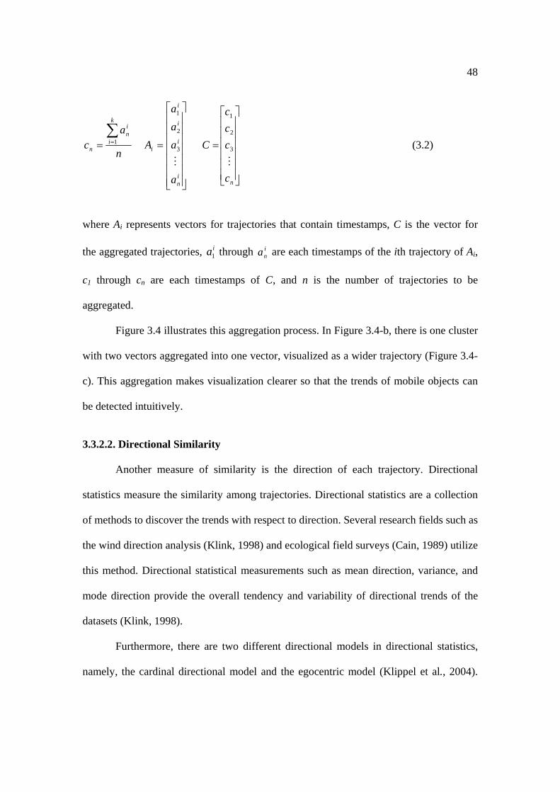
48
⎥⎥⎥⎥⎥⎥
⎦
⎤
⎢⎢⎢⎢⎢⎢
⎣
⎡
=
⎥⎥⎥⎥⎥⎥⎥
⎦
⎤
⎢⎢⎢⎢⎢⎢⎢
⎣
⎡
==∑=
nin
i
i
i
i
k
i
in
n
c
ccc
C
a
a
a
a
An
ac
MM
3
2
1
3
2
1
1
(3.2)
where Ai represents vectors for trajectories that contain timestamps, C is the vector for
the aggregated trajectories, ia1 through ina are each timestamps of the ith trajectory of Ai,
c1 through cn are each timestamps of C, and n is the number of trajectories to be
aggregated.
Figure 3.4 illustrates this aggregation process. In Figure 3.4-b, there is one cluster
with two vectors aggregated into one vector, visualized as a wider trajectory (Figure 3.4-
c). This aggregation makes visualization clearer so that the trends of mobile objects can
be detected intuitively.
3.3.2.2. Directional Similarity
Another measure of similarity is the direction of each trajectory. Directional
statistics measure the similarity among trajectories. Directional statistics are a collection
of methods to discover the trends with respect to direction. Several research fields such as
the wind direction analysis (Klink, 1998) and ecological field surveys (Cain, 1989) utilize
this method. Directional statistical measurements such as mean direction, variance, and
mode direction provide the overall tendency and variability of directional trends of the
datasets (Klink, 1998).
Furthermore, there are two different directional models in directional statistics,
namely, the cardinal directional model and the egocentric model (Klippel et al., 2004).

49
The cardinal directional model describes directions used mainly in cartography such as
north, south, east, and west; it is an objective view, or absolute view, to define the
direction. In contrast, the egocentric directional model describes an individual object’s
heading based on directions such as straight, left, right, back, and so on, which provides
object-centered directional information. As is obvious in Figure 3.6, these two directional
models provide different outputs even when the dataset is same.
This research utilizes both cardinal direction and egocentric direction – the user of
the toolkit can choose either of the directional approaches. The directional statistical
approach classifies trajectories and highlights the trajectories in the same group in the
same color. The average cardinal direction of each trajectory is the sum of the degrees at
each segment between one timestamp and another timestamp (Figure 3.6). This requires
two steps. First, each segment of a trajectory converts itself to be a unit vector to extract
the directional information only. Second, the algorithm calculates the sum of all of the
unit vectors. The degree of the summed vectors is the average cardinal direction. On the
other hand, the algorithm calculating the average egocentric direction uses two segments
from two contiguous timestamps of a trajectory, calculating the change in direction from
the first segment to the second (Figure 3.7). This sum is the average egocentric direction.
Directional statistics help to see the similarity of directions of vectors. After
classifying vector directions in several groups, the vectors in the same group will be
rendered in the same color. This functionality extends the range of data exploration to
examine directional trends and spatial distribution of vectors.

50
3.3.2.3. Geometric Similarity
The third and last measure of similarity is the geometry of mobile objects.
According to Vlachos et al. (2002), there are several issues involved in measuring
geometric similarity. They are as follows:
• Different sampling rates or different speeds
• Similar motions in different locations
• Outliers
• Different lengths
• Efficiency
The first issue relates to the sampled data. There may be some missing portions of
the data in sampling, leading to an inconsistent sampling rate (Vlachos, Kollios, &
Gunopulos, 2002). Moreover, the speed of one mobile object can be faster than another
one. The similarity function, therefore, has to deal with the missing values or inconsistent
speeds. The second issue refers to the fact that the geometry may be similar but the
locations of two or more mobile objects are different, i.e., one trajectory may be a simple
displacement of the other. The similarity function should be consistent regardless of the
locations of mobile objects. The third issue deals with outliers. Anomalies in the sensors
of location-aware devices or human failure can cause this problem. If there are some
outliers, some measures may return extreme values, even though there are only a few
outlier observed locations (Vlachos et al., 2002). The fourth issue, length of the mobile
objects, is a problem that relates to scale. Even though the geometry of mobile objects is
similar, their scale might be different due to differences in trajectory lengths. Therefore,
the similarity function should be a scale-free function, so that it can calculate the

51
similarity of mobile objects with different scales. The fifth issue is the efficiency of the
similarity function. The similarity function has to be adequately expressive but
sufficiently simple, so as to allow for efficient computation.
There has been much research to cope with these challenges. This includes
Dynamic Time Warping (DTW) (McIntosh & Yuan, 2005) and the Longest Common
Subsequence (LCSS) method (Vlachos et al., 2002). DTW focuses on the most dissimilar
parts of the objects, resulting in high sensitivity to noise in the data. On the other hand,
LCSS considers the common portions of the objects. In spatio-temporal analysis, DTW
stretches portions of the sequences to compare transition of locations along the temporal
axis, so the dominant features, patterns of high and low values, are optimally aligned
(McIntosh & Yuan, 2005). Since one of the trajectories always has its location so that the
two trajectories overlap each other for calculation, it is not suitable for large volume
datasets because it is computationally expensive.
There are some other techniques to tackle the issue of measuring similarity:
fractal analysis and shape-based analysis for time-series datasets (Kim, Yoon, Park, &
Kim, 2002). Analysis of the movements of animals and insects often use fractal analysis
(Bascompte & Vila, 1997; Turchin, 1996; With, 1994). In addition, although the latter
kind of research deals with shape-based retrieval, it only deals with time-series analysis
for non-spatial data, such as stock data – it is not applicable to mobile objects.
Another method to extract geometric similarity is to integrate multiple indices of
the object of interest. The combination of characteristics derived from the spatial or
spatio-temporal objects generates new perspectives for pattern detection in data. For
example, McIntosh and Yuan (2005) developed six indices that characterize spatio-
52
temporal objects. They applied the DTW method to temporal sequences of the six indices
to examine the similarity among spatio-temporal events. Another example is Wentz
(2000) that proposed three indices to identify and differentiate one spatial object from
others. Identification and differentiation of spatial objects based on indices of their shape
provides more flexibility to measure shape since those indices address the specific
definition of shape.
This research proposes a geometric similarity function with five indices that
characterize the trajectory of a mobile object. This geometric similarity function requires
three steps: calculation of five indices, conversion of the trajectory into a single point in
an attribute space, and measurement of similarity with a simple distance function. First,
the function extracts five characteristic values of trajectories. They are sinuosity,
direction, velocity, locality, and spatial range. All five indices are essential since a single
index cannot differentiate one trajectory from others. Second, the five indices transform
the trajectory from a polyline into a single point in an attribute space. The attribute space
has five dimensions corresponding to each index, which simplifies the representation of
trajectories. Third, the geometric function calculates the Euclidean distance between two
points: this distance represents the similarity or dissimilarity of trajectories. Figure 3.8
illustrates this in a three-dimensional space for clarity.
If Dg is zero, it indicates that two trajectories are exactly the same in terms of
geometry. In the toolkit, minimum Dg values can be set by the user as the threshold value
to detect groups of similar trajectories for aggregation. Movements of mobile objects that
are similar to each other are rendered in the same color in the visualization (Figure 3.9).
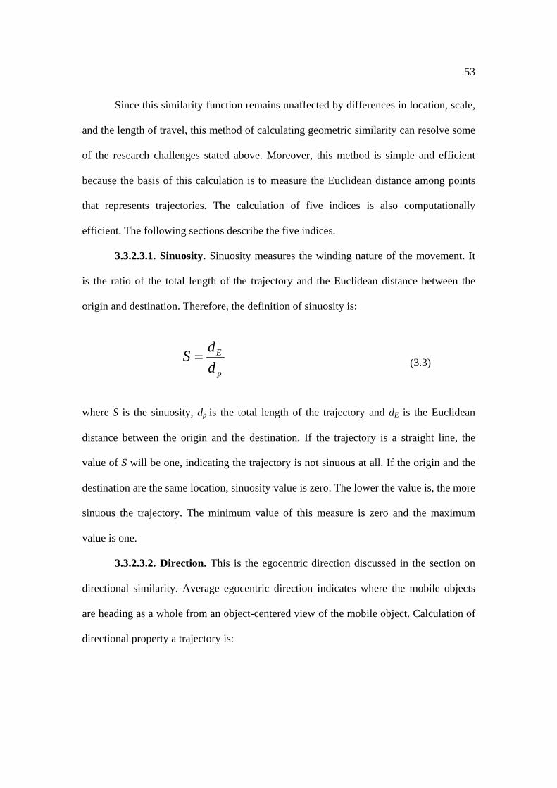
53
Since this similarity function remains unaffected by differences in location, scale,
and the length of travel, this method of calculating geometric similarity can resolve some
of the research challenges stated above. Moreover, this method is simple and efficient
because the basis of this calculation is to measure the Euclidean distance among points
that represents trajectories. The calculation of five indices is also computationally
efficient. The following sections describe the five indices.
3.3.2.3.1. Sinuosity. Sinuosity measures the winding nature of the movement. It
is the ratio of the total length of the trajectory and the Euclidean distance between the
origin and destination. Therefore, the definition of sinuosity is:
p
E
ddS = (3.3)
where S is the sinuosity, dp is the total length of the trajectory and dE is the Euclidean
distance between the origin and the destination. If the trajectory is a straight line, the
value of S will be one, indicating the trajectory is not sinuous at all. If the origin and the
destination are the same location, sinuosity value is zero. The lower the value is, the more
sinuous the trajectory. The minimum value of this measure is zero and the maximum
value is one.
3.3.2.3.2. Direction. This is the egocentric direction discussed in the section on
directional similarity. Average egocentric direction indicates where the mobile objects
are heading as a whole from an object-centered view of the mobile object. Calculation of
directional property a trajectory is:

54
360DDirection= (3.4)
where D is the average direction of a trajectory. The value of Direction ranges from zero
to one since the value of egocentric direction is normalized.
3.3.2.3.3. Velocity. Velocity indicates how fast a mobile object moves during the
time period relative to the maximum velocity in the dataset. Definition of velocity of each
trajectory is as below:
maxVVVelocity = (3.5)
where V is the average velocity of a trajectory, and Vmax is the velocity of one of the
fastest paths in the sample. This value ranges from zero to one. If the value is close to one,
it suggests that the object is moving faster over space relative to the sample.
3.3.2.3.4. Locality. Locality is the ratio of the distance between the origin and the
destination, and the distance between the origin and the farthest location from the origin.
This measure provides information on how far a mobile object moved from the origin in
the whole movement of a trajectory relative to the origin-destination distance (Figure
3.10). This could help distinguish between different types of movements such as
purposeful trips and leisurely tours. It can also distinguish trips that begin and end at the
same location from ones that do not. In detail, it represents how far the objects moved
from the origin compared with the distance between origin and destination:

55
OF
OD
LLLocality = (3.6)
where LOD is the Euclidean distance between the origin and the destination, and LOF is the
distance between the origin and the farthest recorded location from the origin. If the value
is smaller, it indicates that the locations of the origin and the destination are close to each
other, and vice versa. As for the cases of other indices, this value ranges from zero to one.
3.3.2.3.5. Spatial range. Spatial range measures the spatial extent of the
movement. This measure tells how much space is covered by a trajectory. The value is
the area of a convex hull that contains a trajectory divided by the area of the convex hull
that contains all the trajectories that spread all over the study area. The definition of
spatial range is as follows:
all
path
AA
RangeSpatial = (3.7)
where Apath is the area of a convex hull that contains an individual trajectory (Figure 3.11)
and Aall is the area of a convex hull that contains all the visualized trajectories (Figure
3.12). The value ranges from zero to one since this value is normalized by the area that
contains all the trajectories. Therefore, for example, if the trajectory is a straight line,
Apath is zero; if Apath is as large as Aall, the value is one. A spatial range closer to zero
indicates that the trajectory covers relatively little territory, while a spatial range closer to
one indicates a more expansive territory for the object. A convex hull provides a
relatively accurate measure of spatial range (relative to other measures such as the
minimum bounding rectangle) with reasonable computational cost. The Graham scan

56
algorithm has the worst-case time complexity of 0(n log n); this is scalable (Sedgewick,
1990).
3.3.2.3.6. Clustering algorithm for similarity measures. Trajectories that are
considered to be similar to each other are aggregated based on a clustering method. The
trajectories in one cluster are considered to be trajectories with similar characteristics in
either location, direction, or geometry. In the locational similarity function, the average
distance between two trajectories is calculated: the two trajectories are aggregated if the
average distance is smaller than the clustering threshold, which is defined by the user of
the toolkit. In directional and geometric similarity functions, the trajectories are
considered to be in one cluster (or similar movement group) if the directional value or
geometric similarity value is smaller than the clustering threshold. The clustering
algorithm used in this toolkit grows clusters according to a density-based connectivity
analysis – it is called a density-based clustering method (DBSCAN) (Han & Kamber,
2006). The DBSCAN procedure is as follows:
• The neighborhood within a radius ε of a given object is called the ε -neighborhood
of the object.
• If theε -neighborhood of an object contains at least a minimum number, MinPts, of
objects, then the object is called a core object (Figure 3.13).
• Given a set of objects, D, we say that an object p is directly density-reachable from
object q if p is within theε -neighborhood of q, and q is a core object.
• An object p is density-reachable from object q with respect toε and MinPts in a set of
objects, D, if there is a chain of objects p1, …, pn, where p1 = q and pn = p such that
pi+1 is directly density-reachable from pi with respect toε and MinPts, for ni≤≤1 ,

57
Dpi ∈ .
• An object p is density-connected to object q with respect toε and MinPts in a set of
objects, D, if there is an object Do∈ such that both p and q are density-reachable
from o with respect toε and MinPts (Figure 3.14).
This dissertation customizes DBSCAN in three ways. First, the distances for
finding neighbor points are the values calculated between pairs of trajectories by three
similarity functions (location, direction, and geometry). For example, the locational
similarity function calculates the average difference in location between two trajectories.
In this way, the value of locational similarity between two objects is the distance to be
used in DBSCAN. Second, ε , one of two parameters to run the algorithm (MinPts and
ε ), is a user-defined value – as stated above, these two parameters are arbitrary values in
DBSCAN and affect the results dramatically. ε is the threshold value to detect similar
trajectories: the user can try arbitrary values to explore similarity. In data exploration, the
user may not know the appropriate values for this threshold value ε . Thus, simple
statistical values – maximum x coordinate value, minimum x coordinate value, maximum
y coordinate value, minimum y coordinate value – are provided for the data to help guide
the user. On the other hand, the algorithm in this research sets MinPts as one by default,
indicating a cluster can be created by at least two objects – even a pair of trajectories that
are similar to each other can be a group. Third, another parameter is utilized in DBSCAN
in this research – maximum searching radius, MaxE (Figure 3.15). This MaxE determines
the farthest distance to generate clusters from core objects – it is set as a double value of
ε by default. The shape of clusters is constrained by this parameter to include objects
that are within MaxE in one cluster. These parameters, with a combination of similarity

58
functions that are explained in next three sections, provide the interactivity of the
visualization toolkit in this research.
The DBSCAN algorithm requires parameters, the radius ε and MinPts, to be
determined by the user of the algorithm. This is regarded as a disadvantage of DBSCAN
in comparison with other density-based clustering methods such as OPTICS (ordering
points to identify the clustering structure) of which the algorithm determines those
parameters, and DENCLUE (clustering based on density distribution functions), which
requires a set of density distribution functions that require longer computation. However,
since ε is the threshold value of similarity functions in this dissertation, this parameter
can be left as a user-defined parameter, which fits perfectly with the purpose of this
dissertation. The parameter MinPts is set at two because this is the minimum number of
trajectories that are considered to be in one cluster. DBSCAN algorithm is the most
appropriate clustering method for this dissertation.
3.4. Data Summarization
Data summarization methods provide summary information of the visualized
trajectories in the toolkit. There are two components for the summarization methods –
directional statistics and axis conversion. Directional statistics provides overall statistical
information about the trajectories while axis conversion allows the user of the toolkit to
visualize the data from different viewpoints.
3.4.1. Directional Statistics
Directional statistics provide the overall information of visualized trajectories
such as the number of trajectories, mean direction, and mean velocity, which is displayed

59
in the visualization toolkit. These values provide information on trends in the visualized
trajectories.
3.4.2. Axis Conversion
Axis conversion allows the user to explore the visualized trajectories from several
different viewpoints. Visualization is in a three-dimensional view by default, allowing the
user to rotate, zoom-in, zoom-out and pan the visualized trajectories at any viewpoint
using three axes – x, y, and t (time). One option is a typical viewpoint for visualizing
spatial data – two-dimensional space for x and y coordinates. In addition, to examine the
change of x coordinates or y coordinates according to t, the user can select two more
specific viewpoints in the toolkit: an x-t viewpoint and y-t viewpoint (Figure 3.16). In this
way, if the user chooses x and t coordinates, the toolkit visualizes the overall movements
in the x direction according to the time dimension. On the other hand, if the user chooses
y and t coordinates, the toolkit delineates overall movements of the y direction according
to the time dimension.
3.4.3. Data Mining of Geometric Similarity
Data mining techniques within the software WEKA (Witten & Frank, 2005)
utilize geometric similarity indices calculated by geometric similarity functions for
further data exploration of geometric similarity. WEKA consists of major data mining
methods such as association rule mining, classification, and clustering. There is a
component in the toolkit to export the indices from geometric similarity functions, as
well as some other values, into the WEKA format. The indices are ID for each trajectory
(Trajectory ID), ID for groups of the geometric cluster (cluster ID), sinuosity, velocity,

60
spatial range, locality, egocentric direction, cardinal direction, average value of the x
coordinate, and average value of the y coordinate. The user can choose the variables to be
exported by checking the check box in the ‘Export’ section of the toolkit. This option
offers the user another perspective for data exploration by providing data mining analyses
that can afford the means for pattern detection and prediction of the data from nonspatial
data, which will be the integration of Knowledge Discovery in Databases (KDD) and
other visualization toolkits.
3.5. Data Exploration Process
3.5.1. Data Preparation and Import Data into Databases
The next six sections explain the basic process of data exploration with the
visualization toolkit developed in this research. The first step of the data exploration
process is data preparation. There are five required values, namely an ID to identify each
mobile object, date and time of the tracked location, x coordinate, and y coordinate. Data
should be in a text format with a tab delimited form. Second, the toolkit imports the text
data into databases in SQL Server 2005. The user selects the type of datasets, browses to
the text file, and clicks “Import” to store the information in a database.
The database has seven values for each record of locations. These are the
following:
• ID: the identifier used to keep all the records in the database unique. This is the
primary key for the database. The data type is big integer, which can store larger
values than integer.
• trajectoryID: the identifier for each mobile object. Records that have the same
trajectoryID represent records containing locations for one mobile object. The data
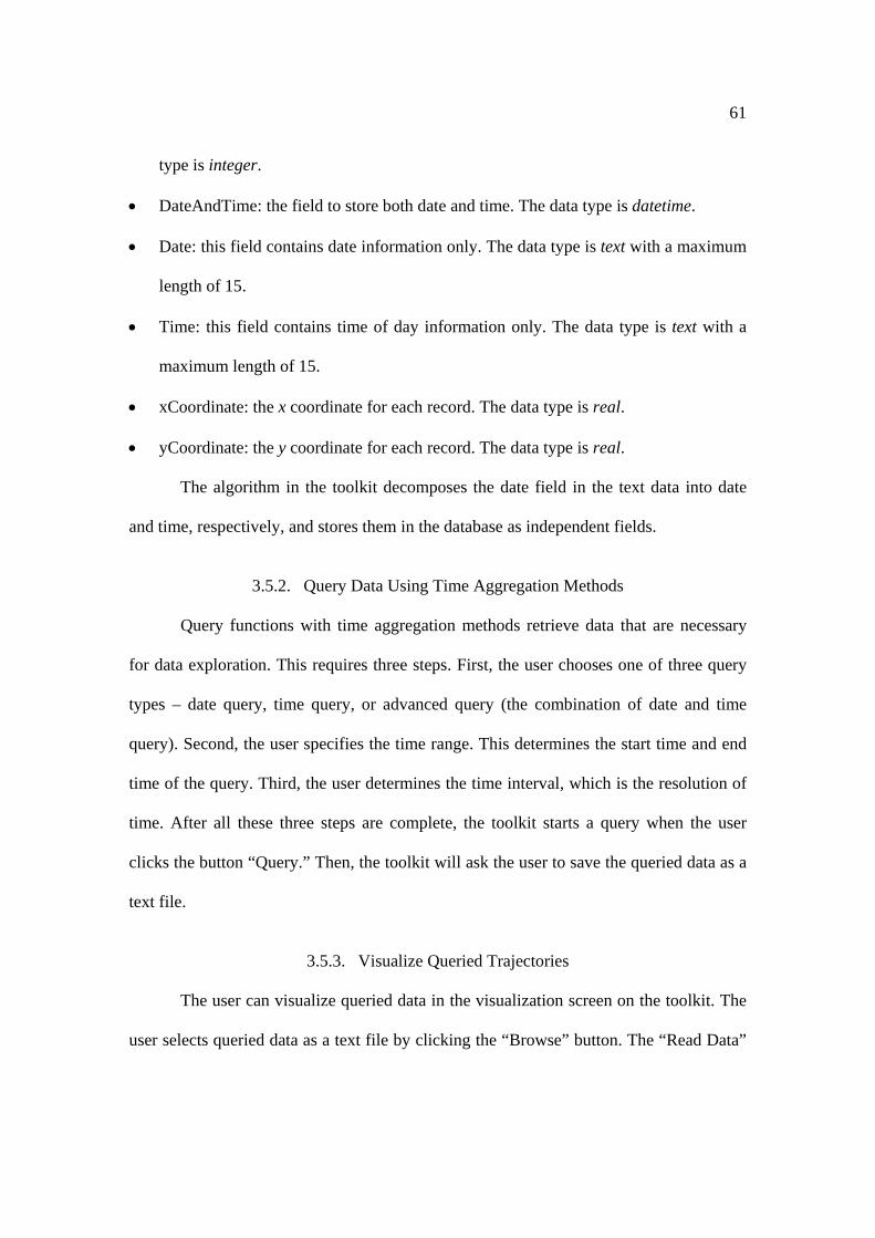
61
type is integer.
• DateAndTime: the field to store both date and time. The data type is datetime.
• Date: this field contains date information only. The data type is text with a maximum
length of 15.
• Time: this field contains time of day information only. The data type is text with a
maximum length of 15.
• xCoordinate: the x coordinate for each record. The data type is real.
• yCoordinate: the y coordinate for each record. The data type is real.
The algorithm in the toolkit decomposes the date field in the text data into date
and time, respectively, and stores them in the database as independent fields.
3.5.2. Query Data Using Time Aggregation Methods
Query functions with time aggregation methods retrieve data that are necessary
for data exploration. This requires three steps. First, the user chooses one of three query
types – date query, time query, or advanced query (the combination of date and time
query). Second, the user specifies the time range. This determines the start time and end
time of the query. Third, the user determines the time interval, which is the resolution of
time. After all these three steps are complete, the toolkit starts a query when the user
clicks the button “Query.” Then, the toolkit will ask the user to save the queried data as a
text file.
3.5.3. Visualize Queried Trajectories
The user can visualize queried data in the visualization screen on the toolkit. The
user selects queried data as a text file by clicking the “Browse” button. The “Read Data”
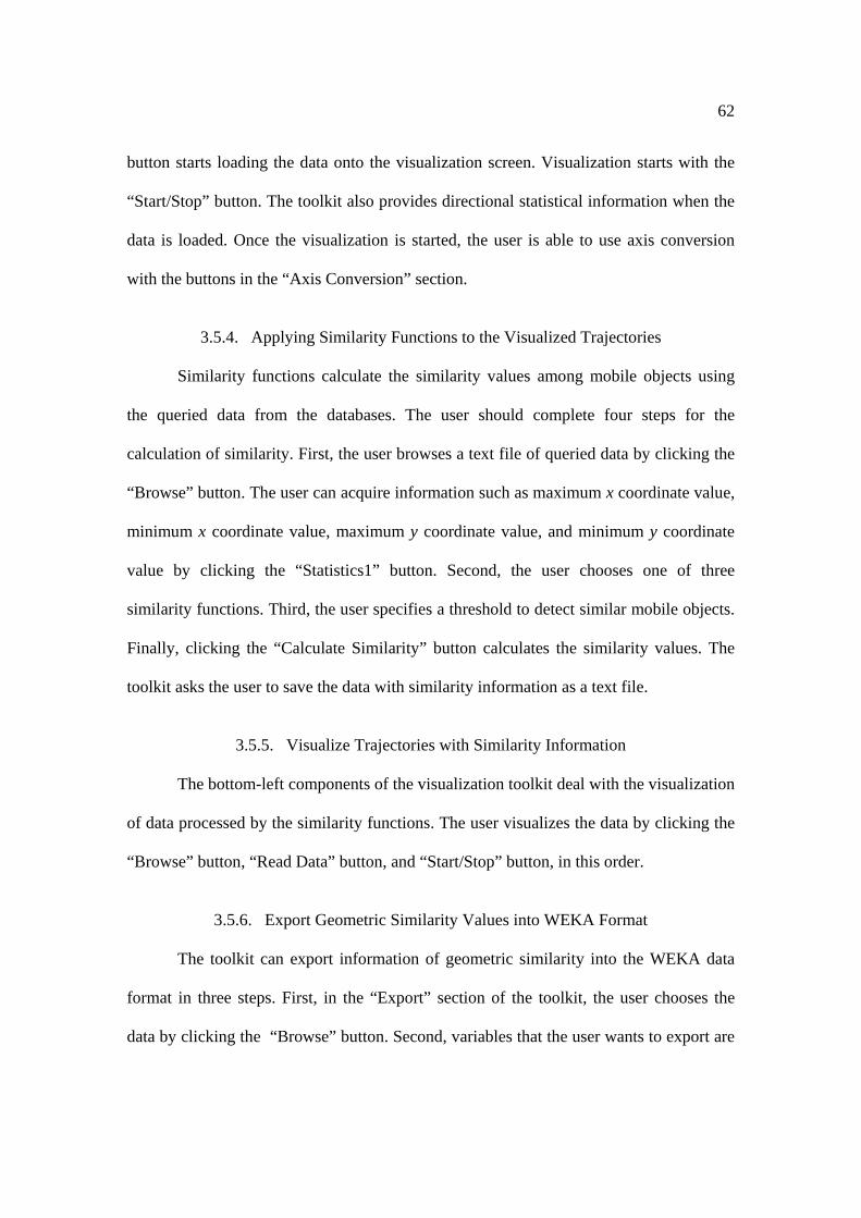
62
button starts loading the data onto the visualization screen. Visualization starts with the
“Start/Stop” button. The toolkit also provides directional statistical information when the
data is loaded. Once the visualization is started, the user is able to use axis conversion
with the buttons in the “Axis Conversion” section.
3.5.4. Applying Similarity Functions to the Visualized Trajectories
Similarity functions calculate the similarity values among mobile objects using
the queried data from the databases. The user should complete four steps for the
calculation of similarity. First, the user browses a text file of queried data by clicking the
“Browse” button. The user can acquire information such as maximum x coordinate value,
minimum x coordinate value, maximum y coordinate value, and minimum y coordinate
value by clicking the “Statistics1” button. Second, the user chooses one of three
similarity functions. Third, the user specifies a threshold to detect similar mobile objects.
Finally, clicking the “Calculate Similarity” button calculates the similarity values. The
toolkit asks the user to save the data with similarity information as a text file.
3.5.5. Visualize Trajectories with Similarity Information
The bottom-left components of the visualization toolkit deal with the visualization
of data processed by the similarity functions. The user visualizes the data by clicking the
“Browse” button, “Read Data” button, and “Start/Stop” button, in this order.
3.5.6. Export Geometric Similarity Values into WEKA Format
The toolkit can export information of geometric similarity into the WEKA data
format in three steps. First, in the “Export” section of the toolkit, the user chooses the
data by clicking the “Browse” button. Second, variables that the user wants to export are

63
selected by checking checkboxes of each variable. Third, clicking the “Export to WEKA
Format” button executes the export action. The saved data are in a WEKA data format
with the extension “.arff.” The user can import the exported WEKA data directly in
WEKA by double-clicking the exported file. The software WEKA is launched, ready to
begin data mining.
3.6. Summary
This chapter introduced the components of the visualization toolkit developed in
this dissertation. Visualization with vector algebra enables a simple but efficient
representation. In addition, aggregation methods for time, location, direction, and
geometry, with user-defined threshold values, provide interactivity and flexibility in data
exploration in order to detect patterns in terms of similarity among trajectories of mobile
objects. Moreover, exporting geometric similarity information to WEKA datasets
connects data mining with Geovisualization. The next chapter of this dissertation
describes the datasets used to illustrate the visualization toolkit.
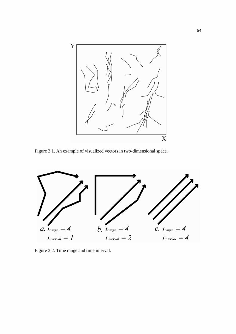
64
Figure 3.1. An example of visualized vectors in two-dimensional space.
Figure 3.2. Time range and time interval.

65
Figure 3.3. Locational similarity.
a. trajectories b. detection of a cluster c. aggregation of trajectories
Figure 3.4. An example of locational vector aggregation.
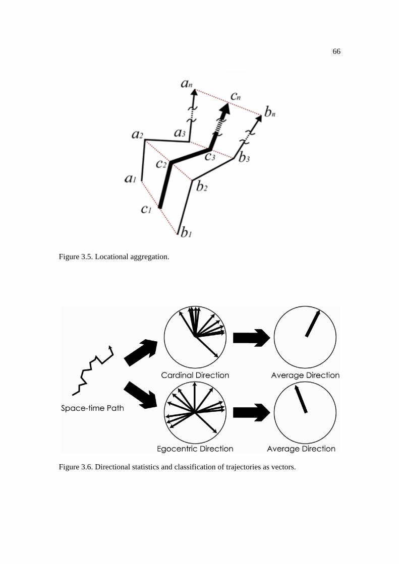
66
Figure 3.5. Locational aggregation.
Figure 3.6. Directional statistics and classification of trajectories as vectors.

67
Figure 3.7. Calculation of egocentric direction.
Figure 3.8. An example of a space-time path as a point using three indices.
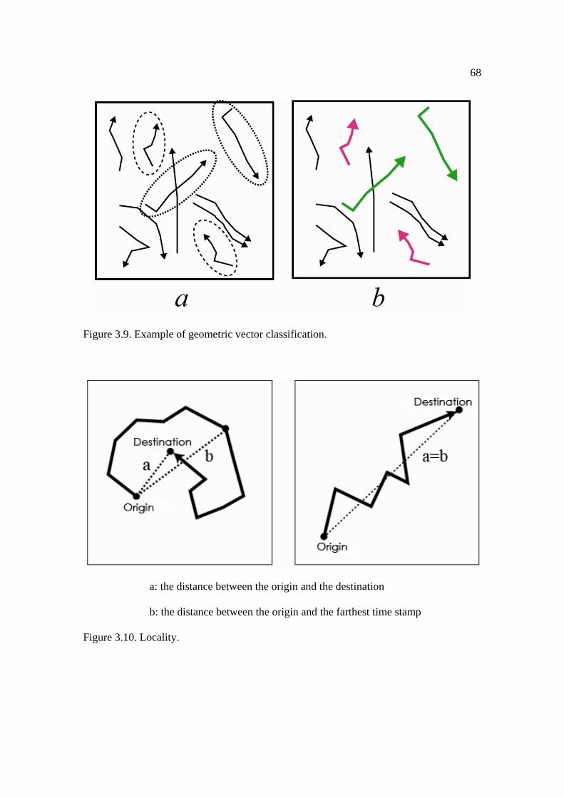
68
Figure 3.9. Example of geometric vector classification.
a: the distance between the origin and the destination
b: the distance between the origin and the farthest time stamp
Figure 3.10. Locality.

69
Figure 3.11. Convex hull of paths.
Figure 3.12. Spatial range.

70
Figure 3.13. Core objects.
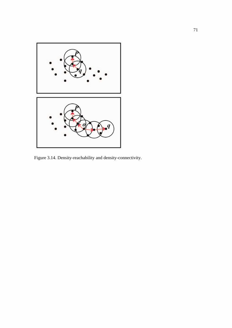
71
Figure 3.14. Density-reachability and density-connectivity.
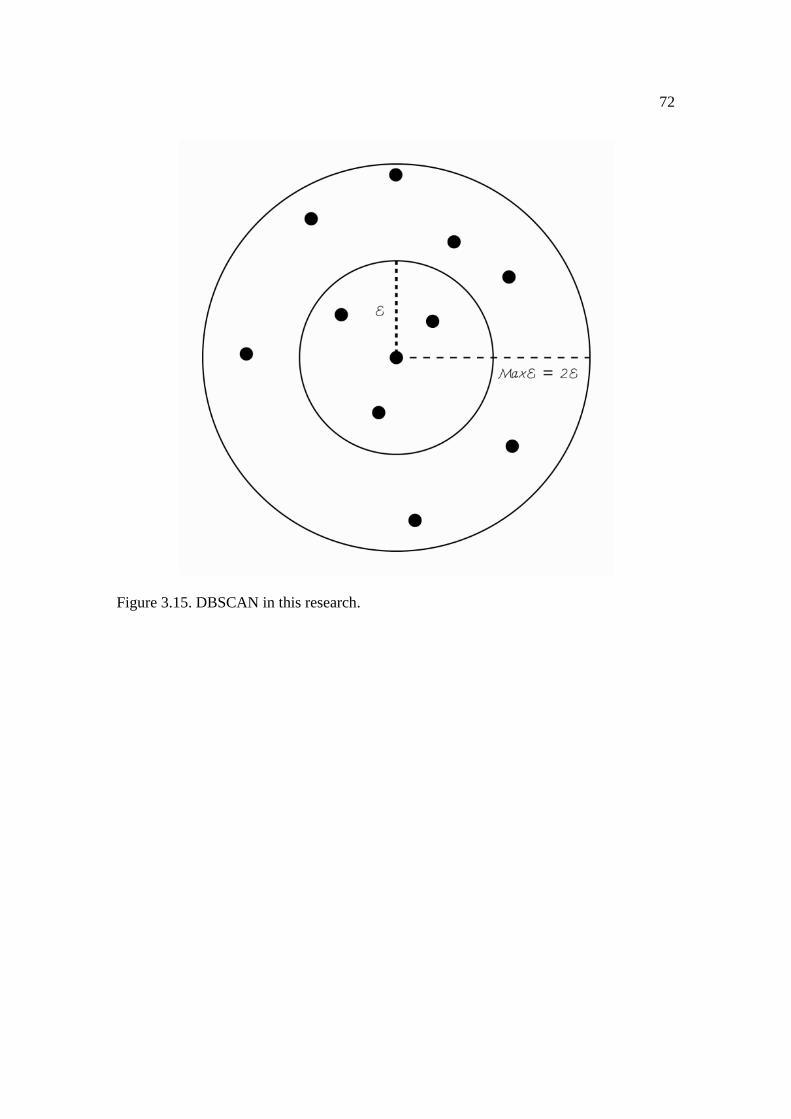
72
Figure 3.15. DBSCAN in this research.

73
Figure 3.16. Axis conversion.

4 DATA
4.1. Overview
This research utilizes datasets consisting of three types of mobile objects data
(MOD): 1) GPS travel survey data in the state of Kentucky, 2) wild chicken movement
data in Thailand, and 3) self-tracking movement data of the investigator in the state of
Utah. Characteristics of movements in each dataset differ from one another because of
the difference in tracking devices, spatial and time resolution of the tracking method,
study area, and so on. In addition, inherent constraints in movements can cause
differences. For example, a road network restricts the movement of vehicles to the
network, while an animal’s movement is more flexible, indicating more free movement
all over the study area. Thus, data exploration with three different datasets identifies the
effectiveness of the visualization toolkit.
4.2. Personal Travel Data Survey in Lexington, Kentucky
Two organizations of the Federal Highway Administration – the Office of
Highway Information Management and the Office of Technology Application –
conducted a project whose purpose was the development and field test of an automated
data collection device that included Global Positioning System (GPS) technology. The
Lexington Area Metropolitan Planning Organization, the principal planning agency for a
two-county area in central Kentucky, volunteered to participate in this project in 1996.

75
The size of study area is approximately 461 square miles with a total population of
approximately 350,000.
The original data consist of four types, namely, activity data, screening interview
data, postdiary interview data, and GPS data. This research utilizes GPS data only. The
date of the recorded timestamps ranges from September 16th to December 30th in 1996.
There are 327,407 timestamps, 89 households, 173 people, and 2,256 trips in total. The
DIGIT Lab of the Department of Geography at the University of Utah created databases
to integrate the information from the four types of data and eliminated the noisy
timestamps for further use. The resulting data contain 290,231 timestamps, 88
households, 163 people, and 1,984 trips. The attribute fields of GPS data in the databases
are household ID, driver’s ID, trip number, sequence number, date, time, longitude,
latitude, and speed in miles per hour. This research uses the driver’s ID, longitude,
latitude, date, and time information.
4.3. Wild Chicken Movement Data in Thailand
The second dataset in this research is movement data of wild chickens in Thailand.
The Human-Chicken Multirelationship Research (HCMR) Project conducted a survey to
collect this data in Chiang Rai, Thailand using Wireless Fidelity (WiFi) positioning
system (Okabe et al., 2006). A small WiFi tag that bundled a chicken’s body recorded the
location and time. The report shows that the effectiveness and usefulness of WiFi
technology can contribute to the growing need to understand the spatial movement of
animals through their trajectories (Turchin, 1998).
The WiFi data tracking system consisted of six devices, namely, tags to stick to
the chickens’ legs, activator, receiver, Power over Ethernet (PoE), WiFi access point, and

76
a management engine. The functionality of each device is as follows. Tags wirelessly
transmited the information of location and time. The weight of the tag was 35 grams and
the size was 62mm×40mm×17mm. The receiver caught the signals from the tags and
transmited the information to the management engine. Three kinds of antennas were used
in the study – 360 degrees, 135 degree, and 60 degrees – due to differences in directional
characteristics. The management engine processed the signal information to track the
location of tags. Spatial resolution was 1 meter and time resolution was 1 second.
The study area was the 200 square-meters of land under cultivation inside the
Chiang Rai Livestock Research and Technology Transfer Center. There were eight
concrete one-storied houses in the area: two of them were residential houses and six of
them were vacant houses. Two of the vacant houses were used as a room to install the
management engine and a preparation room, respectively. The only residents were people
who lived in the two houses. Thus, the chickens could move freely all over the study area.
There were 18 chickens used in this survey – they were the chickens that the
Chiang Rai Livestock Research and Technology Transfer Center owns. There were three
chicken houses in the field: each chicken house contained one cock and five hens. The
survey ran from November 2nd until November 9th in 2005. Preparation of the WiFi
positioning system took place on the 2nd, 3rd, and 4th until 4:30 p.m., which coordinated
the adjustment of the positioning system with the release of the chickens into the field.
Actual data collection started at 4:30 p.m. on the 4th until 9:15 a.m. on the 9th. Okabe et al.
(2006) reported the locational error in the data, indicating that there are directional
patterns in errors. Outliers with extreme locations were eliminated from the data.
77
This research utilizes the data from November 5th to November 8th. To examine
the movement pattern throughout the entire day, this research leaves the data collected on
November 9th out of consideration, since movement was only recorded in the morning for
this date. The attribute information is x coordinate, y coordinate, date, and time.
4.4. Self-tracking Data in Utah
The third dataset is the self-tracking GPS dataset of the investigator. It is a
collection of daily movement data mostly in Salt Lake County, Utah from January 1st,
2007 until December 31st, 2008. A GPS device (Garmin eTrex C) records the timestamps
of everyday movement from the morning until the end of the day. Recording starts when
the investigator first leaves his home and ends when he returns home, which is the last
travel destination of the day. The time resolution is 2 seconds, meaning the GPS records
the location and time every 2 seconds. According to the display on the GPS device, the
minimum spatial error in recording is 4 meters. Since it is impossible to track the
timestamps when the investigator is inside buildings, the GPS only collects movement
outside the buildings. This limitation of tracking causes some issues in data collection.
The GPS device used for this dataset sometimes causes errors in tracking and
generates some missing parts in data. Occasionally, the GPS cannot capture the signals of
satellites because of obstacles such as the density of buildings, bridges, trees, and so on.
Thus, some timestamps are missing or are recorded in unrealistic locations when the
investigator stays at an area where the density of the buildings is high, or an area where
there are many obstacles above the investigator. This happens mostly in the downtown
area of Salt Lake City where tall buildings exist. Another problem is user-error. Some
portions of trajectories are missing because either the investigator forgets to turn on the
78
GPS device or the battery of the GPS device runs out. Thus, there are some days for
which only a part of entire movement is recorded.
Due to the errors and mistakes above, data cleaning is necessary to choose only
days with complete trajectories. In addition, the movement of the investigator outside of
the State of Utah is also eliminated. Elimination of incomplete trajectories and error
locations results in 273 days of complete trajectories. The attributes selected are latitude,
longitude, date, and time.
4.5. Summary
This dissertation utilizes three different datasets for visual data exploration. Each
dataset contains unique movements of mobile objects that can be differentiated from the
movements of other mobile objects. Personal travel data in the state of Kentucky
collected the movement data of a comparatively large number of people. Since each
participant in the survey provided individual movement data for just a few days, an
example of effective analysis may be to seek for the overall patterns or dynamics of the
entire study area as a collection of individual movement. Self-tracking data recorded the
long-term daily movement of one individual. Unlike the other datasets, this dataset
contains movement that starts and ends at the same location for more than 2 years. Data
exploration to investigate the variation in location at different times of a day is a
possibility with this dataset. Although human movements are often limited to road
networks, movements of chickens in Thailand are not limited to a road network. It is
interesting to find original patterns in flexible movement in contrast to the network-
constrained movement. Chapter 5 reports the results of the data exploration with the
visualization toolkit in this research.

5 RESULTS
5.1. Overview
This chapter illustrates the toolkit’s functionalities by showing results from
querying the database at different levels of temporal granularity, and aggregating the
trajectories based on trajectory similarity at the specified granularity. This chapter will
explore results based on the toolkit components described in the Methodology chapter.
Unless otherwise mentioned, this chapter will focus on the Thailand wild chicken dataset,
and use the other datasets to reinforce these results. Note that we only focus on the
functionality of the visualization toolkit aggregation methods, and not on the behavioral
aspects of wild chickens or humans represented by the other databases.
5.2. Aggregation Methods
This section presents results from two aggregation methods: time aggregation and
similarity-based aggregation. As described in the Methodology chapter, the time
aggregation methods allow the user to state a time interval of interest and a time
granularity within that interval to reconstruct individual trajectories at different levels of
movement generality. Given these reconstructed trajectories, the user can then apply
similarity functions to aggregate individual trajectories based on location, direction, and
geometry to generate synthetic trajectories that reflect collective movement patterns at
that scale.
80
5.2.1. Time Aggregation Methods
Figures 5.1 and Figure 5.2 show the effects of time granularity on trajectory
reconstruction. Figure 5.1 illustrates the reconstructed trajectory collection for three
different time ranges (6:00 –9:00, 6:00 – 12:00, and 6:00 – 17:00) at the native time
interval provided by the data (1 second). Figure 5.2 illustrates the reconstructed trajectory
collection at three time intervals for a fixed time range from 6:00 to 17:00. As Figure 5.1
suggests, it is difficult to extract distinct patterns at the highest level of temporal
granularity. Even at a relatively low time range, the trajectory collection is generally an
undistinguished mass. This problem becomes more acute as the time range increases.
Figure 5.2 indicates that changing the time interval can mitigate this problem to a
substantial degree: the trajectories are more generalized and patterns are more easily
discernable as the time intervals become coarser. The visualization toolkit allows the user
to visualize the trajectory collection at the time range of interest and interactively change
the time interval until an appropriate granularity level is achieved for the data and
questions at hand.
This visual simplification is similar with other datasets. Figure 5.3 is the example
of Lexington GPS mobility patterns with four different time granularities: 1 second, 10
seconds, 1 minute and 10 minutes. As is the case of Figure 5.2, a coarser time interval
simplifies visualized trajectories, except for the central part where trajectories are dense.
Although oversimplification with an extremely high value of time interval can obscure
the movement patterns, the appropriate time interval value can simplify the visualization
and uncover patterns in trajectory datasets.

81
5.2.2. Similarity Functions
5.5.2.1. Locational Similarity
After the user has selected the time range and interval, the toolkit allows for the
aggregation of similar trajectories to detect clearer patterns from the data. In addition to
the time aggregation methods illustrated in the previous sections, similarity functions can
uncover patterns in the trajectories. Figure 5.4 compares the visualization from Figure 5.1
(three images of the top row) and the trajectory similarities based on a relatively relaxed
locational similarity threshold of 10.0 (three images of the bottom row). Note that as the
time range increases, visualization of the disaggregated data becomes more complicated,
and it becomes hard to detect visual patterns without the use of similarity functions.
However, obvious patterns emerge when applying a similarity function. The locational
similarity function detects three distinct groups in all three time ranges. To validate the
consistency of this trend, we assessed the number of groups of visualized data while
systemically increasing the time range by 1 hour in each step. The number of groups of
this dataset is constantly three throughout the day, except for 4 groups emerging between
6:00 and 8:00. This implies the stability of mobility patterns across time in this dataset.
Although the locational similarity function facilitates the pattern detection process,
it can also oversimplify the visualization since it aggregates similar trajectories into a
single one. Figure 5.5 shows the result from the Lexington mobility data of trajectories
aggregated by the locational similarity function. As the locational similarity value
increases, small and short-length aggregated trajectories in different groups concentrate
in one area, which makes patterns difficult to discern. Some datasets are sensitive to the
similarity measures, thus the user must carefully choose the threshold value of the

82
similarity functions in order to find nominal patterns.
It is also possible to compare aggregated trajectories across different time ranges
to explore for recurrent or stable patterns across longer time frames. Figure 5.6 illustrates
mobility patterns across different dates using the same time ranges. The top row shows
the movement for 1 day only (November 5th, 2005) with respect to different time ranges,
while the bottom row illustrates mobility patterns for those same time ranges aggregated
across all 4 days (November 5th, 2005 to November 8th, 2005). This functionality allows
the user to explore for recurrent behavior (i.e., mobility behavior that occurs within the
same time ranges across different days or similar time periods). In both cases, there are
three groups of similar movement that are remarkably stable whether we view these
patterns within 1 day or across multiple days. This suggests the existence of recurrent
mobility patterns in this database.
The locational similarity function is useful for finding patterns of movement in
urban areas. Figure 5.7 illustrates the daily movement of the investigator in the morning
and the afternoon time period. In each image, the investigator’s house is at the bottom-
left location and the University of Utah is at the top-right location. The locational
similarity function successfully detects similar trajectories from the investigator’s home
to the University of Utah, detecting the generic commuting patterns of the investigator.
The investigator uses four major routes to commute to the University of Utah. The
locational similarity function detects four aggregated trajectories that depart from the
bottom-left and end at the top-right. Each aggregated trajectory represents a summarized
route for commuting to the University of Utah.
The combination of time aggregation methods and similarity functions enables
83
comparisons of movement at the same cyclical time period in different years. Figure 5.8
is the comparison of the investigator’s daily movement over a 4-month period (from
September to December) in 2007 (top row images) and 2008 (bottom row images). The
locational similarity function is applied to both datasets. Although the time-of-year
period is the same, detected patterns are distinctly different: movement in 2007 has
several clusters and is wide in the rage of movement, while the movement in 2008 has
fewer clusters with simpler movement patterns.
The time range can also focus on detailed movement throughout 1 day. Figure 5.9
shows three different 1-hour periods for the movement of wild chickens. Some clustered
movement can be found in the visualization without similarity functions (top row images)
while clusters clearly appear with locational similarity functions (bottom row images).
Visualization with shorter time ranges enables the user to focus on detailed movement:
the user can find patterns relatively easily. Similarity functions, in this case, show the
clusters that can also be found in the visualization without similarity functions to
reinforce the visual exploration.
The time range can also illustrate interesting patterns of human mobility. Figure
5.10 shows two different 1-hour segments of the investigator’s movement. Visualization
without applying the similarity function (top row images) already shows the frequent
routes on the road network by the density of trajectories at similar locations. In addition,
visualization with the locational similarity function (bottom row images) detects clusters,
which clearly appear to summarize the movement in each time range.
Figure 5.11 shows the visualization of chicken movement across all 4 days using
two different time intervals and two different threshold values for locational similarity.

84
The four visualizations, arranged as a quadrant at the left side of Figure 5.11, show the
movement of chickens at a time interval of 5 seconds. In contrast, four visualizations in a
quadrant on the right side of Figure 5.11 show the same data at a time interval of 10
minutes. The upper row shows results from a locational similarity threshold of 0.1 (a
value that requires high similarity for trajectory aggregation) while the lower row shows
results from a locational similarity threshold of 10.0 (a value that requires less similarity).
Figure 5.11 distinguishes trajectories with locational similarity using different colors.
Note the affects of time interval granularity on the ability to discern patterns. The
individual trajectories in the upper row are dense and difficult to disentangle into clear
patterns. The individual trajectories in the lower row, at a coarser temporal interval level,
are more visually manageable. Also note the affects of locational similarity thresholds on
the visual patterns. The upper row indicates the difficulty in finding general patterns
when requirements for locational similarity threshold are high: no trajectories are
candidates for aggregation. However, the bottom row shows three distinct groups that
emerge when the locational similarity is less severe. In addition, these similarity groups
remain stable across the two levels of temporal interval granularity. This suggests, in this
case, we discovered synoptic mobility patterns that are robust and can be effectively
summarized using a coarser time interval that provides a simple and more easily
understood view of the data, compared to a finer temporal interval.
5.2.2.2. Directional Similarity
The second similarity function is based on directional information. The
directional similarity function detects similar trajectories with respect to two types of
directions (egocentric direction and cardinal direction) and renders the trajectories in the

85
same cluster into the same color (unlike the locational similarity function, the directional
similarity function does not aggregate trajectories). Figure 5.12 shows the comparison of
1-day (November 5th, 2005) and 4-day (from November 5th to November 8th, 2005)
directional mobility patterns of wild chickens. Visualization without the directional
similarity function (left-most column images) and visualization with egocentric similarity
values of 1.0, 10.0, and 30.0 are in Figure 5.12. A relaxed directional similarity value
(right-most column images) detects a few clusters at similar locations (mostly in red and
green) while a strict directional similarity value detects more clusters with some outliers.
Similar patterns can be found in two different time ranges, implying consistency within
the movement patterns of chickens with respect to direction.
Figure 5.13 and Figure 5.14 show movement patterns with egocentric similarity in
two different time ranges (6:00 – 9:00 and 6:00 - 12:00) in different date ranges. Figure
5.13 illustrates the 4-day (from November 5th to November 8th, 2005) movement
patterns while Figure 5.14 illustrates 1 day’s (November 5th, 2005) movement patterns.
As time range increases from 6:00 – 9:00 to 6:00 - 12:00 in Figure 5.13, visualization
without similarity functions becomes complicated. However, notable patterns appear
when a directional similarity function is applied. As is the case of Figure 5.12, a relaxed
egocentric similarity value detects a few clusters while a strict similarity value detects
clusters in more detail. In addition, data with a longer time range (6:00 – 12:00) have
more outliers. Similar results are shown in Figure 5.14, but more detail cluster formation
can be detected because there are fewer trajectories. Also, more outliers are detected with
a strict similarity value.
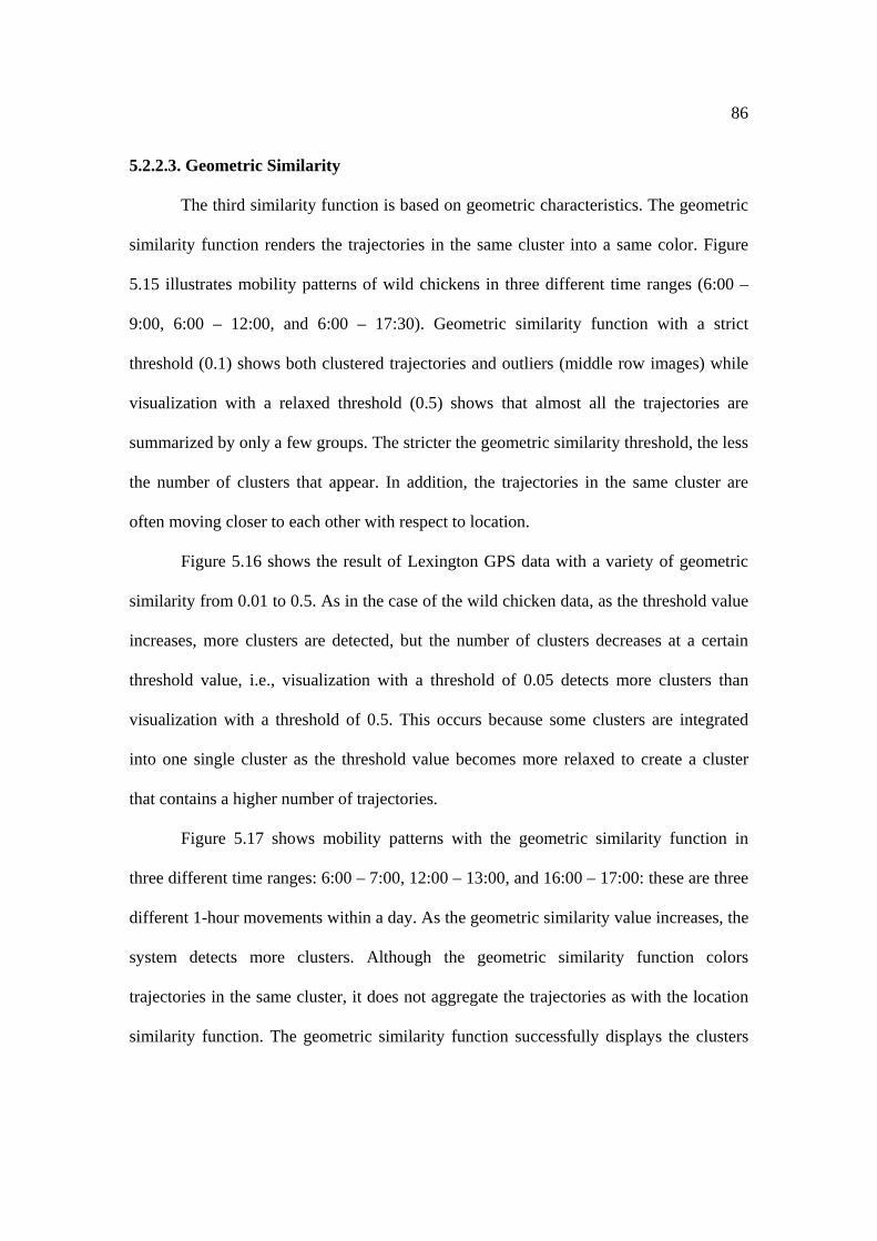
86
5.2.2.3. Geometric Similarity
The third similarity function is based on geometric characteristics. The geometric
similarity function renders the trajectories in the same cluster into a same color. Figure
5.15 illustrates mobility patterns of wild chickens in three different time ranges (6:00 –
9:00, 6:00 – 12:00, and 6:00 – 17:30). Geometric similarity function with a strict
threshold (0.1) shows both clustered trajectories and outliers (middle row images) while
visualization with a relaxed threshold (0.5) shows that almost all the trajectories are
summarized by only a few groups. The stricter the geometric similarity threshold, the less
the number of clusters that appear. In addition, the trajectories in the same cluster are
often moving closer to each other with respect to location.
Figure 5.16 shows the result of Lexington GPS data with a variety of geometric
similarity from 0.01 to 0.5. As in the case of the wild chicken data, as the threshold value
increases, more clusters are detected, but the number of clusters decreases at a certain
threshold value, i.e., visualization with a threshold of 0.05 detects more clusters than
visualization with a threshold of 0.5. This occurs because some clusters are integrated
into one single cluster as the threshold value becomes more relaxed to create a cluster
that contains a higher number of trajectories.
Figure 5.17 shows mobility patterns with the geometric similarity function in
three different time ranges: 6:00 – 7:00, 12:00 – 13:00, and 16:00 – 17:00: these are three
different 1-hour movements within a day. As the geometric similarity value increases, the
system detects more clusters. Although the geometric similarity function colors
trajectories in the same cluster, it does not aggregate the trajectories as with the location
similarity function. The geometric similarity function successfully displays the clusters

87
that can be easily found by visual exploration. For these data, the summary trajectories
are persistent across all three time ranges; this suggests distinct spatial behavior types that
are stable across time.
Figure 5.18 illustrates trajectory collections at a moderate geometric similarity
threshold combined with different levels of temporal granularity and spatial projections
to the two-dimensional plane. The time range is fixed at 10 seconds. Again, note the
affect of temporal granularity on the visual legibility of the individual mobility patterns,
even with trajectory aggregations. Mobility patterns at the 10-minute granularity provide
an elegant synoptic view of three groups with similar movement with respect to trajectory
geometry: these patterns are much easier to detect compared to results at the finer level of
temporal granularity. However, in this case, the discovered mobility patterns are
substantially different at the two levels of temporal granularity. This suggests a higher
sensitivity of geometric similarity to temporal granularity than locational similarity. It
also suggests the value of exploring these aggregations at different levels of temporal
interval granularity in order to determine the robustness of the discovered patterns. It is
also notable that differences are more apparent with respect to movement in the y-
dimension over time.
5.3. Data Summarization
Data summarization enhances the effectiveness of visual exploration in two
components: directional statistical information and axis conversion. Statistical
information summarizes the information of visualized data while axis conversion
provides functionality to view the data from various viewpoints.
88
5.3.1. Directional Statistics
The statistical information reported by the system has two parts: geographic
extent of x and y coordinates of visualized trajectories (statistics 1), and summarized
information of trajectories (statistics 2): number of trajectories, number of detected
clusters, mean velocity, and mean direction (Figure 5.19). These two components are
useful respectively. For example, outliers or errors of recorded location can be found with
the combination of visualization and statistics 1 information (Figure 5.20). The user can
edit the data to remove the errors and visualize the data without outliers. In addition,
numbers of clusters are easily found by statistics 2 information, even though the
visualized trajectories appear to be complicated (Figure 5.21). Visual exploration can be
leveraged with the assistance of statistical information.
5.3.2. Data Mining of Geometric Similarity Indices
Another functionality of the visualization toolkit is a data mining functionality
that enables the user to export geometric similarity indices (sinuosity, velocity, egocentric
direction, cardinal direction, locality, spatial range) that can be analyzed in other data
mining software. This research utilizes the data mining software WEKA for decision tree
analysis, which is one of the classification methods, with the purpose of discovering the
rules that describe the movement of wild chickens. The decision tree algorithm J48 is
used to create a tree to discover attributes that influence cluster detection with the
geometric similarity function. J48 is based on the C4.5 algorithm: C4.5 is one of the most
widely used algorithms for decision tree induction (Han & Kamber, 2006).
This decision tree analysis is conducted on datasets with different time
aggregation and geometric similarity aggregation settings. For example, Table 5.1 shows

89
the data mining result of wild chicken data in various time ranges: three 1-hour period
movements (top three rows in the table, i.e., 6:00 - 7:00, 12:00 - 13:00, and 16:00 -
17:00) and three incremental time ranges (bottom three rows in the table, i.e., 6:00 - 9:00,
6:00 - 12:00, and 6:00 - 17:30). Time interval and geometric similarity threshold are
constant in all the time range cases: the time interval is 10 seconds and the geometric
similarity threshold is 0.5. The root node identifies the prominent factor in the resulting
decision tree: egocentric direction is the root node in all cases. This indicates that
egocentric direction is the most significant index to determine the movement patterns. In
addition, the percentage of correctly classified instances is higher when the time range
becomes longer (bottom three rows): longer time movement may be more predictable
than short time movement. Furthermore, similarity tendency is obvious with the number
of clusters detected in visualization (this is the number of clusters detected by the
geometric similarity function) and the percentage of correctly classified instances. The
fewer number of clusters we have, the higher percentage classified correctly.
Table 5.2 summarizes the results of decision tree analysis of self-tracking data
with several time ranges: the same decision trees were generated as in the case of wild
chickens. The number of observations in this case (88 to 273 observations) is greater than
wild chicken cases (18 observations). As with the case for wild chickens, egocentric
direction is the root node in all of the examined cases. This is constantly obvious in the
cases of the Lexington data in Table 5.3, which summarizes results of the decision tree
analysis of the Lexington mobility data with several time ranges. In addition, the
percentage of correctly classified instances is constantly higher than 90.00%, except for
one case, even though the number of instances and number of clusters detected by the
90
geometric similarity measure are higher. Egocentric direction may be one of the critical
variables to be considered in discovering mobile object movement patterns.
Time interval is another variable that can affect the data mining result. Table 5.4
summarizes the decision tree analysis results of wild chicken data with two different
geometric similarity thresholds (0.1 and 0.5) and five different time intervals (5 seconds,
10 seconds, 1 minute, 10 minutes and 30 minutes). Table 5.5 illustrates the results with
self-tracking data with four geometric similarity values (0.1, 0.5, 1.0, and 2.0). In the
results of wild chicken cases, datasets with relaxed geometric similarity (0.5) and with
coarser time interval (10 minutes and 30 minutes) did not obtain any results because there
is only one cluster as a result of geometric similarity aggregation. In addition, the dataset
with a relaxed geometric similarity measure (0.5) received a higher percentage score of
correctly classified instances. This similar trend can be found in the cases of self-tracking
data. This occurs due to the decrease in the number of clusters as the geometric similarity
threshold increases; it is simpler to classify the instances with a fewer number of clusters.
Moreover, the dataset with this geometric similarity (0.5) received the same results even
though the time interval changed from 5 seconds to 1 minute, indicating consistency in
movement patterns. Furthermore, egocentric direction is the root node of decision trees in
wild chicken cases. However, other indices such as spatial range and sinuosity are the
root nodes in the cases of self-tracking mobility data and the cases of Lexington data
(Table 5.6). This implies the possibility of the time interval having a significant influence
on the results of data mining.
Examination of the decision tree itself is another important aspect of decision tree
analysis. Decision trees of self-tracking data in four different time ranges (0:00 – 9:00,
91
0:00 – 12:00, 0:00 – 18:00, 0:00 – 24:00) illustrate that the size of the tree grows as the
time range stretches with an increasing number of leaves. As is shown in Table 5.2, the
root node is egocentric direction. The next most important explanatory factor is sinuosity
in all the cases except for the case of the time range of 0:00 – 24:00: in this case, the
spatial range is a factor in the second level. This implies the consistency of the mobility
patterns because egocentric direction and sinuosity are the two key factors that describe
the movement of self-tracking data.
Decision trees for the self-tracking data in another four different time ranges (6:00
– 9:00, 9:00 – 12:00, 12:00 – 15:00, 15:00 – 18:00) show a tendency similar to the
decision trees of self-tracking data in four different time ranges (0:00 – 9:00, 0:00 –
12:00, 0:00 – 18:00, 0:00 – 24:00): egocentric direction is the root node and sinuosity is
at the second level in most cases. As the time ranges change, the size of the tree and
number of leaves varies. For example, the tree shape in the time range of 6:00 – 9:00 and
12:00 – 15:00 are exactly same: there may be similar mobility patterns with respect to
geometry occurring in these two time ranges. In addition, the size of the tree in the time
range of 6:00 – 9:00 and 12:00 – 15:00 are small in contrast with other time ranges. This
may explain why the complexity of the movement differs from one time range to another:
the percentage of correctly classified instances in the tree of the time range of 6:00 – 9:00
(96.59%) and 12:00 – 15:00 (96.39%) are higher than the other two time ranges – time
range of 9:00 – 12:00 (90.96%), and that of 15:00 – 18:00 (91.01%) (see Table 5.2).
Decision trees of self-tracking data with three geometric similarity thresholds (0.1,
0.5, and 1.0) show that the size of trees becomes smaller since the number of clusters
detected by geometric similarity functions becomes smaller: a relaxed similarity function

92
threshold (1.0) includes a larger number of trajectories in one cluster and therefore, the
function detects fewer clusters. In these three cases, the shapes of decision trees are quite
different from each other: the root node is not egocentric direction all the time. Clearly,
threshold values can greatly impact the results of data mining.
5.4. Summary
This chapter described the functionality of the visualization toolkit with examples
from three mobile object datasets. Vector algebra, time aggregation methods, and
similarity functions provide effective visual exploration of the mobile objects data. In
addition, data summarization methods such as axis conversion and statistical information
support the user of the toolkit for more comprehensive understanding of the visualized
mobile objects. Furthermore, data mining with WEKA enables the exploration of rules
that describe the movement patterns. Chapter 6 discusses the contributions of this
research, contribution to other research efforts, and future research challenges.
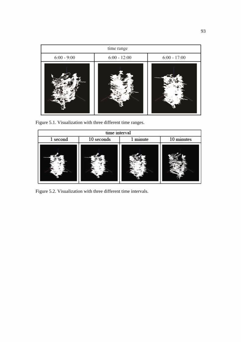
93
Figure 5.1. Visualization with three different time ranges.
Figure 5.2. Visualization with three different time intervals.

94
Figure 5.3. Visualization of Lexington data with different time intervals.
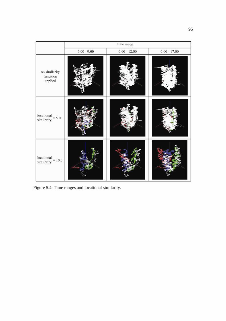
95
Figure 5.4. Time ranges and locational similarity.

96
Figure 5.5. Oversimplification with locational similarity.
Figure 5.6. Locational similarity and time ranges across different dates.

97
Figure 5.7. Locational similarity with self-tracking data within 1 day.
Figure 5.8. Comparison of movement at the same period in 2 different years.

98
Figure 5.9. Locational similarity and time range within 1 day.

99
Figure 5.10. Locational similarity and self-tracking movement in the morning time period.

100
Figure 5.11. Temporal granularity and locational similarity.
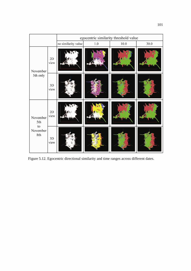
101
Figure 5.12. Egocentric directional similarity and time ranges across different dates.
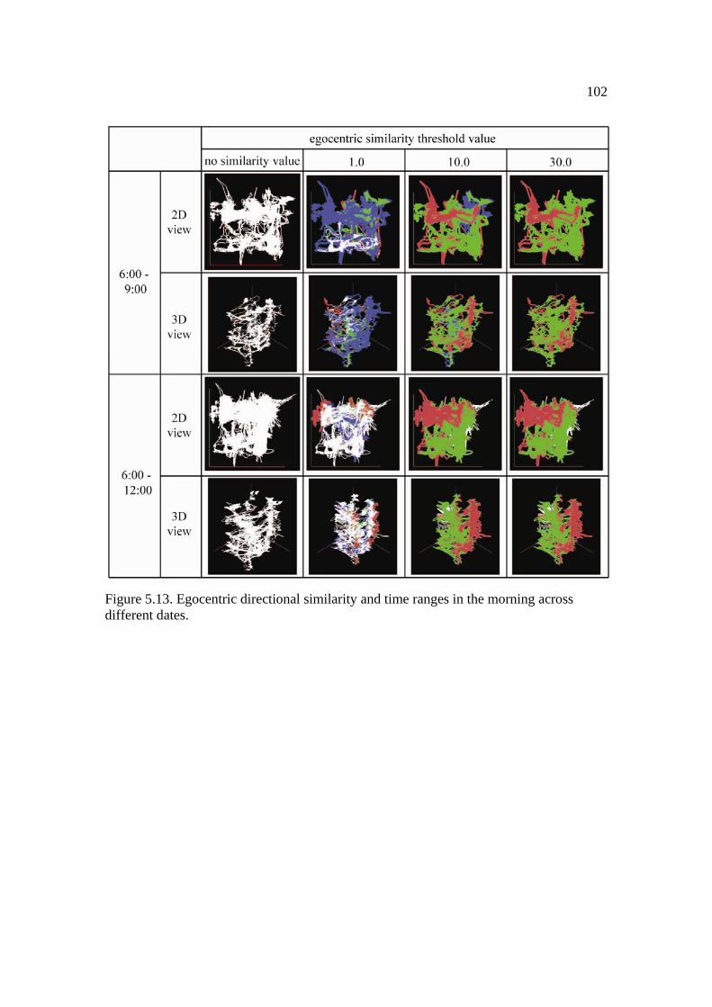
102
Figure 5.13. Egocentric directional similarity and time ranges in the morning across different dates.
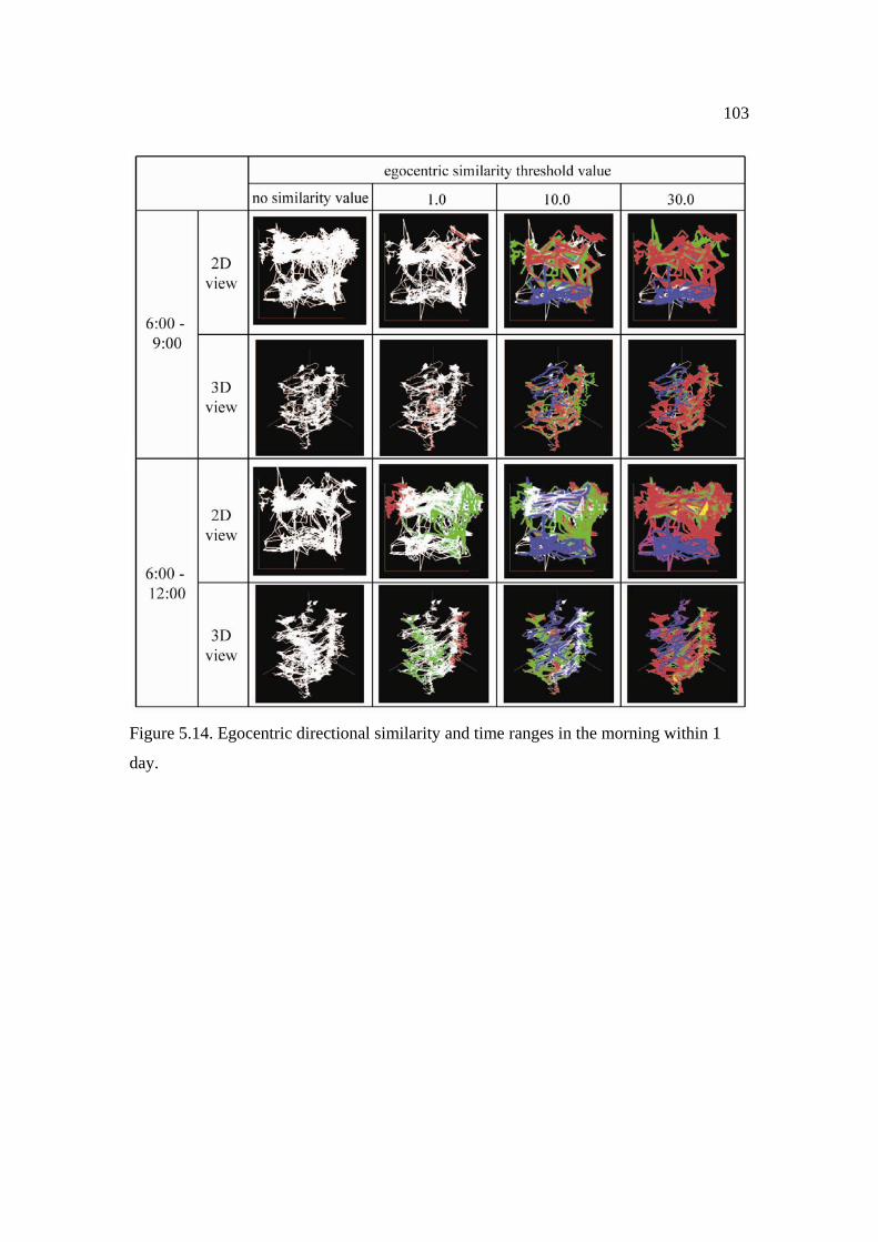
103
Figure 5.14. Egocentric directional similarity and time ranges in the morning within 1
day.

104
Figure 5.15. Time range and geometric similarity.
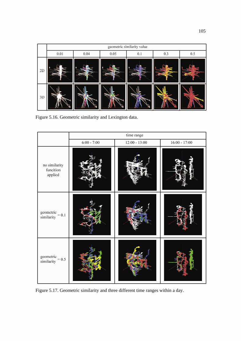
105
Figure 5.16. Geometric similarity and Lexington data.
Figure 5.17. Geometric similarity and three different time ranges within a day.

106
Figure 5.18. Axis conversion and geometric similarity.

107
Figure 5.19. Statistical information.
Figure 5.20. Outlier detection and refined visualization.

108
Figure 5.21. Number of clusters detected with statistical information.
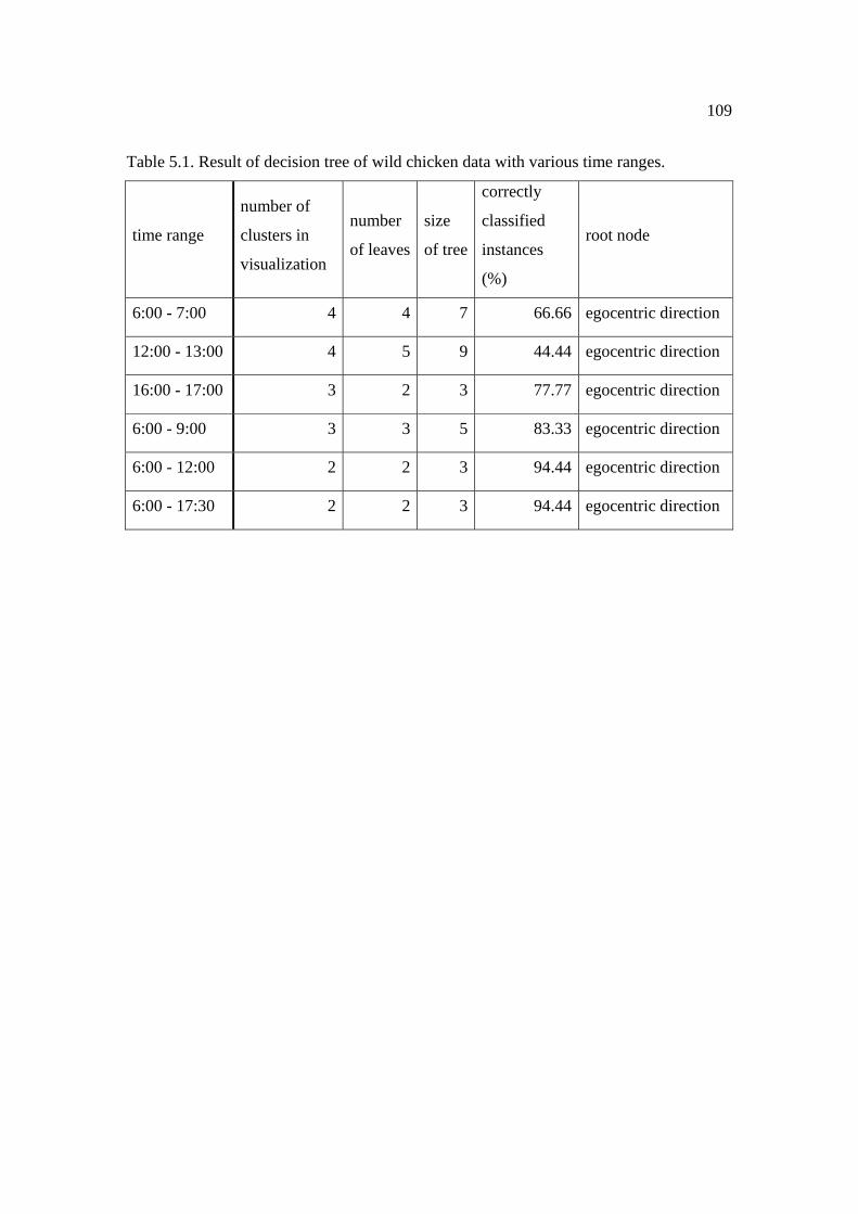
109
Table 5.1. Result of decision tree of wild chicken data with various time ranges.
time range
number of
clusters in
visualization
number
of leaves
size
of tree
correctly
classified
instances
(%)
root node
6:00 - 7:00 4 4 7 66.66 egocentric direction
12:00 - 13:00 4 5 9 44.44 egocentric direction
16:00 - 17:00 3 2 3 77.77 egocentric direction
6:00 - 9:00 3 3 5 83.33 egocentric direction
6:00 - 12:00 2 2 3 94.44 egocentric direction
6:00 - 17:30 2 2 3 94.44 egocentric direction
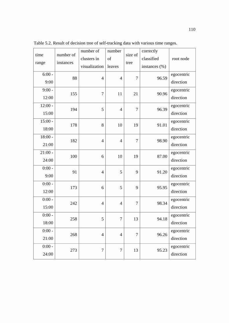
110
Table 5.2. Result of decision tree of self-tracking data with various time ranges.
time
range
number of
instances
number of
clusters in
visualization
number
of
leaves
size of
tree
correctly
classified
instances (%)
root node
6:00 -
9:00 88 4 4 7 96.59
egocentric
direction
9:00 -
12:00 155 7 11 21 90.96
egocentric
direction
12:00 -
15:00 194 5 4 7 96.39
egocentric
direction
15:00 -
18:00 178 8 10 19 91.01
egocentric
direction
18:00 -
21:00 182 4 4 7 98.90
egocentric
direction
21:00 -
24:00 100 6 10 19 87.00
egocentric
direction
0:00 -
9:00 91 4 5 9 91.20
egocentric
direction
0:00 -
12:00 173 6 5 9 95.95
egocentric
direction
0:00 -
15:00 242 4 4 7 98.34
egocentric
direction
0:00 -
18:00 258 5 7 13 94.18
egocentric
direction
0:00 -
21:00 268 4 4 7 96.26
egocentric
direction
0:00 -
24:00 273 7 7 13 95.23
egocentric
direction

111
Table 5.3. Result of decision tree of Lexington data with various time ranges.
time range number of
instances
number of
clusters in
visualization
number
of leaves
size of
tree
correctly
classified
instances
(%)
root node
6:00 - 9:00 60 4 10 19 66.67 sinuosity
6:00 - 12:00 95 3 8 15 54.73 egocentric
direction
6:00 - 18:00 134 16 26 51 47.76 egocentric
direction
6:00 - 24:00 141 13 25 49 65.24 egocentric
direction
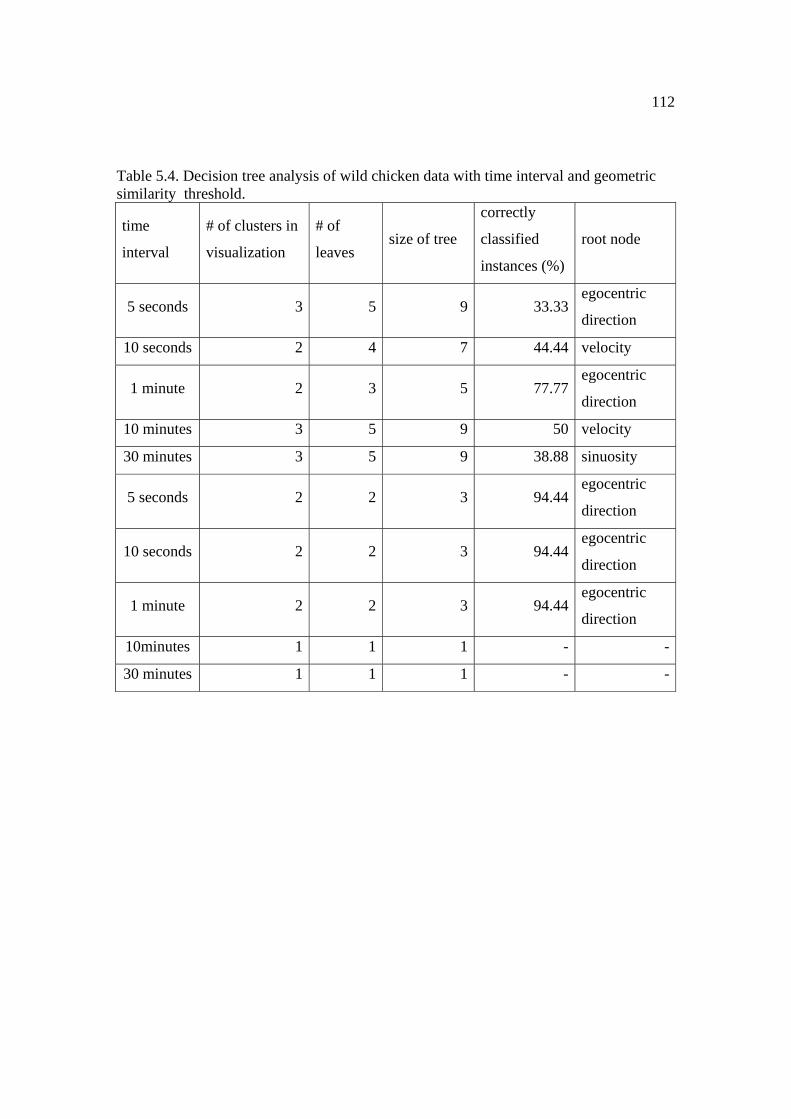
112
Table 5.4. Decision tree analysis of wild chicken data with time interval and geometric similarity threshold.
time
interval
# of clusters in
visualization
# of
leaves size of tree
correctly
classified
instances (%)
root node
5 seconds 3 5 9 33.33 egocentric
direction
10 seconds 2 4 7 44.44 velocity
1 minute 2 3 5 77.77 egocentric
direction
10 minutes 3 5 9 50 velocity
30 minutes 3 5 9 38.88 sinuosity
5 seconds 2 2 3 94.44 egocentric
direction
10 seconds 2 2 3 94.44 egocentric
direction
1 minute 2 2 3 94.44 egocentric
direction
10minutes 1 1 1 - -
30 minutes 1 1 1 - -
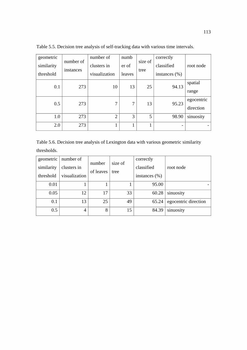
113
Table 5.5. Decision tree analysis of self-tracking data with various time intervals.
geometric
similarity
threshold
number of
instances
number of
clusters in
visualization
numb
er of
leaves
size of
tree
correctly
classified
instances (%)
root node
0.1 273 10 13 25 94.13 spatial
range
0.5 273 7 7 13 95.23 egocentric
direction
1.0 273 2 3 5 98.90 sinuosity
2.0 273 1 1 1 - -
Table 5.6. Decision tree analysis of Lexington data with various geometric similarity
thresholds.
geometric
similarity
threshold
number of
clusters in
visualization
number
of leaves
size of
tree
correctly
classified
instances (%)
root node
0.01 1 1 1 95.00 -
0.05 12 17 33 60.28 sinuosity
0.1 13 25 49 65.24 egocentric direction
0.5 4 8 15 84.39 sinuosity

6 DISCUSSION AND CONCLUSION
Chapter 6 reviews the major contents of this research (section 6.1.) and its
scientific contributions to related research fields (section 6.2). Section 6.3 discusses
future research challenges and possible improvements and enhancements with respect to
the research objectives stated in the beginning of this research. This chapter ends with
some concluding remarks.
6.1. Summary
This research aimed to create a highly interactive visualization toolkit to uncover
interesting patterns in large volume mobile objects data (MOD). Functionalities such as
time aggregation methods with similarity functions synthesize and summarize the overall
movement trends in the data. Various combinations of time aggregation parameters and
similarity function thresholds successfully detected clusters that extract similar mobility
patterns at a specific time scale. In addition, vector representation, statistical information,
and axis conversion supported visual data exploration to understand the movement
patterns with complicated visualized mobile objects. Moreover, this toolkit connected
MOD to data mining software for further data exploration. Results from decision tree
analysis vary based on the combination of time aggregation parameters and similarity
function thresholds.
115
6.2. Contributions
The research presented contributes to the scientific and mobile object databases
communities in several main areas: 1) high interactivity of visualization toolkit for
knowledge discovery in MOD; 2) synthesis of time aggregation and similarity measures;
and 3) ability to handle large volume MOD. The toolkit created in this research allows
the user to explore MOD in various ways: the user can determine parameters for each
functionality of the toolkit. This high interactivity of a visualization toolkit enables visual
and geocomputational analysis in flexible and ad-hoc ways. Existing data summarization
techniques such as online analytical processing (OLAP) and time aggregation methods
(Hornsby & Egenhofer, 2002), and data mining analysis are combined with similarity
functions that are presented in this research for deeper data exploration that are especially
suitable for MOD.
The second contribution is a synthesis of time aggregation methods and similarity
measures. Time aggregation methods and similarity measures are often treated as
different topics in mobile objects research. However, it is important to handle both
aspects since the analysis mobile objects requires temporal, spatial, and shape
information to be analyzed at the same time. Combination of time aggregation methods
and similarity functions reveal that the careful choice of time aggregation parameters and
similarity thresholds significantly influence the visual results. It is important to utilize
both a temporal aspect and a similarity aspect for the advanced and detailed analysis of
mobility patterns. In addition, because the geometric similarity function requires
geometric components only, it has the ability to compare the similarity of two or more
mobile objects at different location and spatial scales. Geometric similarity measure

116
provides a robust way to measure similarity regardless of differences in location and
scale: these two elements are major barriers for geographic analysis that are difficult to
overcome.
The ability to handle large volume MOD is the final contribution. The
visualization toolkit presented demonstrated results for three kinds of mobile objects that
are small (18 objects of wild chickens) to large (273 objects of self-tracking data) in size.
The visualization toolkit successfully analyzed all three kinds of data, starting from
querying the data from the databases and ending with data mining analysis in WEKA
software. In addition to the ability to handle datasets computationally, the toolkit
facilitated the visual exploration of large volume datasets with time aggregation and
similarity functions that provide summarized and simpler visualized MOD. The toolkit
provides essential features for the exploratory data analysis of MOD.
6.3. Future Research Development
Future research challenges that derive from this research can be summarized in
four categories: 1) consideration of behavioral contexts of mobile objects; 2)
development of other similarity measures; 3) validation of visual exploration; and 4)
evaluation of the effectiveness of the methods to other MOD.
6.3.1. Consideration of Behavioral Contexts of Mobile Objects
Chapter 5 of this research demonstrated the functionalities of the visualization
toolkit and resulting outcomes from the computational and visual exploration. However,
this research focuses only on the effectiveness of functionalities in the toolkit to show the
ability to find mobility patterns: behavioral contexts of mobile objects that can be

117
explained from the found patterns are neglected. Studying the relationship between
behavioral aspects of mobile objects and detected patterns is a broader research question.
It is common knowledge in behavioral science and transportation research fields
that specific types of behavior, such as commuting behavior and recreational behavior,
have unique characteristics. It is important to analyze the mobility data of specific types
of behavior with the toolkit developed in this research to analyze the outstanding patterns
in the behavior. For example, time aggregation methods can extract the commuting
behavior in the morning time range and the evening time range, respectively, with the
time interval of interest. Visualization of each time range will provide the mobility
patterns of each commuting behavior in several time scales. In addition, similarity
functions will detect similar mobility patterns and outliers in the commuting behavior.
There may be certain routes in the urban area that many mobile objects pass at a similar
time period. The locational similarity function can detect this behavior. On the other hand,
outliers that are not clustered by similarity functions may lead to the discovery of new
routes for commuting that can mitigate traffic congestion. Analysis of specific types of
behavior is a next step for this research.
Detection of specific types of behavior from large volume datasets is another
possible extension with the toolkit described in this research. As mentioned in the
previous paragraph, certain types of behavior, such as commuting behavior, occur at the
certain time periods, such as in the morning or in the evening. It is possible to assume
when those specific types of behavior occur and try to extract them using time
aggregation methods. Following analysis with similarity functions can provide the
patterns of the extracted mobility data. Functionalities in the toolkit in this research can

118
contribute to behavioral sciences in the new era of data-rich research.
6.3.2. Development of Other Similarity Measures
Although the similarity functions in this research are scalable and effective at
detecting similar mobility patterns, there are many ways to assess trajectory similarity.
Other ways of measuring locational, directional, and geometric similarity should be
explored, as well as other definitions of trajectory similarity distinct from the two
dimensions explored in this research.
One possible way is to examine the properties that can be extracted from
trajectories. There are other characteristics that can be calculated from trajectories other
than the five properties identified in this research, such as average travel distance,
average x coordinate location and y coordinate location of a trajectory, and so on.
Behavioral characteristics such as number of activities, number of visiting locations, and
activity duration time are also possibilities. It is important to evaluate these
characteristics as potential key factors to uncover interesting patterns in MOD.
The investigator has extended this work to create a toolkit that enables visual
exploration of trajectory properties in the attribute space in conjunction with the
geographic space (see Figure 6.1). This toolkit allows for how the values of each property
of a trajectory may change over time (the visualization component at the center in the
toolkit described in Figure 6.1). The bottom graphs illustrate the changes of each value
with respect to time. Visualization components on the left side show two-dimensional
and three-dimensional geographic views of trajectories. The user can incorporate any
other characteristics of trajectory to examine the change in values using this toolkit,
which may lead to the discovery of key factors that describe mobility patterns of MOD.

119
6.3.3. Validation of Visual Exploration
In addition, it is difficult to validate the patterns detected solely by visualization
because found patterns are based on human visual intuition. Since intuitive
comprehension can be misleading, it is urgent to develop methods to validate the detected
patterns.
Utilizing geocomputational techniques is one of the solutions to complement the
results from visual exploration. Pattern detection techniques such as classification and
clustering may be useful to find rules in MOD, which provides a different perspective
other than the visual intuitive interpretation of data. In this research for example, data
mining analysis with decision trees aimed to find the rules that describe mobility patterns,
which provided that the egocentric direction is the most important explanatory factor in
many cases. Data mining analysis and visual exploration complement each other in
knowledge discovery and validation of the visual exploration.
6.3.4. Evaluation of the Effectiveness of the Methods to Other MOD
Furthermore, it is important to test the effectiveness of the granularity and
aggregation methods to other special cases of mobility patterns such as individual
people’s movement inside buildings, migrating birds, and so on. Since each mobile object
has its unique constraints, unique movement patterns may be detected. Applied analysis
using time and similarity aggregation methods will reveal the usability and weakness of
aggregation methods in different applications, which can lead to the development of more
powerful methods to analyze MOD.
120
6.4. Conclusion
As the volume and complexity of MOD increases with the growing usage of
digital mobile devices, there is a high demand for developing new techniques to handle
and analyze the emerging data. Existing techniques are incomplete due to their lack of
ability to handle large volume data. This research developed a highly interactive
visualization toolkit for large volume MOD for exploratory visual and geocomputational
data exploration that can lead to knowledge discovery in individual-based mobility
patterns.
Existing research provides techniques to analyze MOD, such as time aggregation
methods with OLAP, similarity measures to detect similar mobility patterns, and so on.
However, these techniques are often computationally expensive and not well integrated.
The toolkit developed in this research responds to a need for a more synthetic way to
analyze MOD; it accomplishes this by integrating various techniques into one toolkit.
Visualization with computational techniques enhances the range of exploratory data
analysis. The toolkit also has the ability to handle large volume datasets, which
overcomes one of the major research challenges in the literature.
Although the toolkit detected some interesting patterns, the true success of the
toolkit is whether the data exploration will lead to meaningful knowledge discovery for
applied fields such as transportation planning, behavioral modeling, and evacuation
planning in a time of disaster. These fields can benefit from the pattern detection process
proposed in this research for hypothesis generation, model creation, and planning.
Development of methods to bridge visualization and knowledge discovery techniques

121
with applied geographic phenomena will facilitate the decision-making processes that
lead to better policy making and planning.

LITERATURE CITED
Andrienko, G., & Andrienko, N. (2008). Spatio-temporal aggregation for visual analysis
of movements. IEEE Symposium on Visual Analytics Science and Technology (VAST), 51-58.
Andrienko, G., Andrienko, N., Fischer, R., Mues, V., & Schuck, A. (2006). Reactions to geovisualization: An experience from a European project. International Journal of Geographic Information Science, 20(10), 1149-1171.
Andrienko, G., Andrienko, N., & Gatalsky, P. (2005). Impact of data and task characteristics on design of spatio-temporal data visualization tools. In J. Dykes, A. MacEachren, & M.-J. Kraak (Eds.), Exploring geovisualization (pp. 201-222). Oxford, UK: Elsevier Ltd.
Andrienko, G., Andrienko, N., & Wrobel, S. (2007). Visual analytics tools for analysis of movement data. ACM SIGKDD Explorations Newsletter 9(2), 38-46.
Bascompte, J., & Vila, C. (1997). Fractals and search paths in mammals. Landspace Ecology, 12(4), 213-221.
Bédard, Y., & Han, J. (2009). Fundamentals of spatial data warehousing for geographic knowledge discovery. In H. J. Miller & J. Han (Eds.), Geographic data mining & knowledge discovery (pp. 45-68). Boca Raton, FL: CRC Press.
Bian, L. (2004). A conceptual framework for an individual-based spatially explicit epidemiological model. Environment and Planning B: Planning and Design, 31, 381-395.
Bowman, J. l., & Ben-Akiva, M. E. (2001). Activity-based disaggregate travel demand model system with activity schedules. Transportation Research Part A, 35, 1-28.

123
Brewer, C. A. (1997). Spectral schemes: Controversial color use on maps. Cartography and Geographic Information Science, 24(4), 203-220.
Brimicombe, A., & Li, Y. (2006). Mobile space-time envelopes for location-bsed services. Transactions in GIS, 10(1), 5-23.
Brodlie, K. (2005). Models of collaborative visualization. In J. Dykes, A. MacEachren, & M.-J. Kraak (Eds.), Exploring geovisualization (pp. 463-475). Oxford, UK: Elsevier Ltd.
Buckley, A., & Hardy, P. (2007). Cartographic software capabilties and data requirements: Current status and a look toward the future. Cartography and Geographic Information Science, 34(2), 155-157.
Buliung, R. N., & Kanaroglou, P. S. (2004). On design and implementation of an object-relational spatial database for activity/travel behaviour research. Journal of Geographical Systems, 6, 237-262.
Cain, M. L. (1989). The analysis of angular data in ecological field studies. Ecology, 70(5), 1540-1543.
Cheng, T., & Li, Z. (2006). A multiscale approach for spatio-temporal outlier detection. Transactions in GIS, 10(2), 253-263.
Coors, V., Elting, C., Kray, C., & Laakso, K. (2005). Presenting route instructions on mobile devices: From textual directions to 3D visualization. In J. Dykes, A. MacEachren, & M.-J. Kraak (Eds.), Exploring geovisualization (pp. 529-550). Oxford, UK: Elsevier Ltd.
Crampton, J. W. (2002). Interactivity types in geographic visualization. Cartography and Geographic Information Science, 29(2), 85-98.
Demšar, U. (2007). Combining formal and exploratory methods for evaluation of an exploratory geovisualization application in a low-cost usability experiment. Cartography and Geographic Information Science, 34(1), 29-45.
Dennison, P. E., K.Q. Halligan, & D.A. Roberts. (2004). A comparison of error metrics and constraints for multiple endmember spectral mixture analysis and spectral angle mapper. Remote Sensing of Environment, 93, 359-367.

124
DiBiase, D. (1990). Visualization in the earth sciences. Earth and Mineral Science, Bulletin of the College of Earth and Mineral Sciences, Penn State University, 59(2), 13-18.
Dykes, J., MacEachren, A. M., & Kraak, M.-J. (2005). Exploring geovisualization. Oxford, UK: Elsevier Ltd.
Dykes, J., Moore, K., & Wood, J. (1999). Virtual environments for student fieldwork using networked components. International Journal of Geographical Information Science, 13(4), 397-416.
Dykes, J. A., & Mountain, D. (2003). Seeking structure in records of spatio-temporal behaviour: Visualization issues, efforts and applications. Computational Statistics & Data Analysis, 43, 581-603.
Erwig, M., Guting, R. H., Schneider, M., & Vazirgiannis, M. (1999). Spatio-temporal data types: An approach to modeling and querying moving objects in databases. GeoInformatica, 3(3), 269-296.
Fabrikant, S. I. (2000). Spatialized browsing in large data archives. Transactions in GIS, 4(1), 65-78.
Fabrikant, S. I. (2001, August 6-10). Visualizing region and scale in information spaces. Paper presented at the Proceedings of The 20th International Cartographic Conference (ICC 2001), Beijing, China.
Fabrikant, S. I., Montello, D. R., Ruocco, M., & Middleton, R. S. (2004). The distance-similarity metaphor in network-display spatializations. Cartography and Geographic Information Science, 31(4), 237-252.
Fabrikant, S. I., & Skupin, A. (2005). Cognitively plausible information visualization. In J. Dykes, A. MacEachren, & M.-J. Kraak (Eds.), Exploring geovisualization (pp. 667-690). Oxford, UK: Elsevier Ltd.
Fayyad, U. M. (1996). From data mining to knowledge discovery: An overview. In U. M. Fayyad (Ed.), Advances in knowledge discovery and data mining (pp. 2-34). Menlo Park, CA: The MIT Press.
125
Frihida, A., Marceau, D. J., & Theriault, M. (2002). Spatio-temporal object-oriented data model for disaggregate travel behavior. Transactions in GIS, 6(3), 277-294.
Fuhrman, S., Ahonen-Rainio, P., Edsall, R. M., Fabrikant, S. I., Koua, E. L., Tobon, C., et al. (2005). Making useful and usable geovisualization: Design and evaluation issues. In J. Dykes, A. MacEachren, & M.-J. Kraak (Eds.), Exploring geovisualization (pp. 553-566). Oxford, UK: Elsevier Ltd.
Fuhrman, S., & Pike, W. (2005). User-centered design of collaborative geovisualization tools. In J. Dykes, A. MacEachren, & M.-J. Kraak (Eds.), Exploring geovisualization (pp. 591-609). Oxford, UK: Elsevier Ltd.
Gahegan, M. (2005). Beyond tools: Visual support for the entire process of GIScience. In J. Dykes, A. MacEachren, & M.-J. Kraak (Eds.), Exploring geovisualization (pp. 83-99). Oxford, UK: Elsevier Ltd.
Gahegan, M. (2009). Visual exploration and explanation in geography - analysis with light. In H. J. Miller & J. Han (Eds.), Geographic data mining and knowledge discovery (2nd ed., pp. 291-324). Boca Raton, FL: CRC Press.
Gahegan, M., Takatsuka, M., Wheeler, M., & Hardisty, F. (2002). Introducing GeoVISTA Studio: An integrated suite of visualization and computational methods for exploration and knowledge construction in geography. Computers, Environment and Urban Systems, 26, 267-292.
Gahegan, M., Wachowicz, M., Harrower, M., & Rhyne, T.-M. (2001). The integration of geographic visualization with knowledge discovery in databases and geocomputation. Cartography and Geographic Information Science, 28(1), 29-44.
Golledge, R. (2002). The nature of geographic knowledge. Annals of Association of American Geographers, 92(1), 1-14.
Golledge, R., & Stimson, R. J. (1997). Spatial behavior: New York, NY: The Guilford Press.
Guo, D., Chen, J., MacEachren, A., & Liao, K. (2005). A visual inquiry system for space-time and multivariate patterns (VIS-STAMP). IEEE Transactions on Visualization and Computer Graphics, 12(6), 1461-1474.

126
Guo, D., Gahegan, M., MacEachren, A. M., & Zhou, B. (2005). Multivariate analysis and Geovisualization with an integrated geographic knowledge discovery approach. Cartography and Geographic Information Science, 32(2), 113-132.
Guo, D., Liao, K., & Morgan, M. (2007). Visualizing patterns in a global terrorism incident database. Environment and Planning B: Planning and Design, 34, 767-784.
Guting, R. H., & Schneider, M. (2005). Moving objects databases. San Francisco, CA: Morgan Kaufman.
Hagerstrand, T. (1970). What about people in Regional Science? Papers of the Regional Science Association, 24, 7-21.
Hall, R. W. (1983). Travel outcome and performance: The effect of uncertainty on accessibility. Transportation Research Part B, 17B(4), 275-290.
Han, J., Lee, J.-G., & Kamber, M. (2009). An overview of clustering methods in geographic data analysis. In H. J. Miller & J. Han (Eds.), Geographic data mining and knowledge discovery (2nd ed., pp. 149-188). Boca Raton, FL: CRC Press.
Hendricks, M. D., Egenhofer, M. J., & Hornsby, K. (2003). Structuring a wayfinder's dynamic space-time environment. Lecture Notes in Computer Science, 2825, 75-92.
Hopfer, S., & MacEachren, A. (2007). Leveraging the potential of geospatial annotations for collaboration: A communication theory perspective. International Journal of Geographic Information Science, 21(8), 921-934.
Hornsby, K. (2001). Temporal zooming. Transactions in GIS, 5(3), 255-272.
Hornsby, K., & Cole, S. (2007). Modeling moving geospatial objects from an event-based perspective. Transactions in GIS, 11(4), 555-573.
Hornsby, K., & Egenhofer, M. J. (2002). Modeling moving objects over multiple granularities. Annals of Mathematics and Artificial Intelligence (36), 177-194.
Huang, Y., Chen, C., & Dong, P. (2008, September 23-26, 2008). Modeling herds and their evolvements from trajectory data. Paper presented at the Proceedings of The

127
5th International Conference on Geographic Information Science (GIScience 2008), Park City, UT, USA.
Imfeld, S. (2000). Time, points and space - Towards a better analysis of wildlife data in GIS. Doctoral dissertation, University of Zurich, Switzerland.
Jonsen, I. D., Myers, R. A., & Flemming, J. M. (2003). Meta-analysis of animal movement using state-space models. Ecology, 84(11), 3055-3063.
Kaasinen, E. (2003). User needs for location-aware mobile services. Personal and ubiquitous computing, 7(1), 70-79
Kapler, T., & Wright, W. (2005). GeoTime information visualization. Information Visualization, 4, 136-146.
Kareiva, P. M., & Shigesada, N. (1983). Analyzing insect movement as a correlated random walk. Oecologia, 56, 234-238.
Kim, S.-W., Yoon, J., Park, S., & Kim, T.-H. (2002). Shape-based retrieval of similar subsequences in time-series databases. Paper presented at the The 2002 ACM Symposium on Applied Computing, Madrid, Spain.
Kirwan, B., & Ainsworth, L. K. (1992). A guide to task analysis. Boca Raton, FL: CRC Press.
Klink, K. (1998). Complementary use of scalar, directional, and vector statistics with an application to surface winds. Professional Geographer, 50(1), 3-13.
Klippel, A., Dewey, C., Knauff, M., Richter, K. F., Montello, D. R., Freksa, C., et al. (2004). Directional concepts in wayfinding assistance systems. Workshop on Artificial Intelligence in Mobile Systems 2004 (AIMS'04), Saarbrücken: SFB 378, Memo 84, 1-8.
Kraak, M.-J. (2003). The space-time cube revisited from a geovisualization perspective. Paper presented at the Proceedings of The 21th International Cartographic Conference. Durban, South Africa.
Kraak, M.-J., & MacEachren, A. (1999). Visualization for exploration of spatial data. Internatioanl Journal of Geographic Information Science, 13(4), 285-287.
128
Kuijpers, B., Moclans, B., Othman, W., & Vaisman, A. (2009). Analyzing trajectories using uncertainty and background information. Lecture Notes in Computer Science, 5644, 135-152.
Kwan, M.-P. (1999). Gender and individual access to urban opportunities: A study using space-time measures. Professional Geographers, 51(2), 210-227.
Kwan, M.-P. (2000). Interactive geovisualization of activity-travel patterns using three-dimensional geographical information systems: A methodological exploration with a large data set. Transportation Research C(8), 185-203.
Kwan, M.-P., & Weber, J. (2003). Individual accessibility revisited: Implications for geographical analysis in the twenty-first century. Geographical Analysis, 35(4), 341-353.
Laube, P., Dennis, T., Forer, P., & Walker, M. (2007). Movement beyond the snapshot - Dynamic analysis of geospatial lifelines. Computers, Environment and Urban Systems, 31, 481-501.
Laube, P., Duckham, M., & Wolle, T. (2008, September 23-26). Decentralized movement pattern detection amongst mobile geosensor nodes. Paper presented at the Proceedings of The 5th International Conference on Geographic Information Science (GIScience 2008), Park City, UT, USA.
Laube, P., Imfeld, S., & Weibel, R. (2005). Discovering relative motion patterns in groups of moving point objects. International Journal of Geographic Information Science, 19(6), 639-668.
Laurini, R., Servigne, S., & Tanzi, T. (2001). A primer on TeleGeoProcessing and TeleGeoMonitoring. Computers, Environment and Urban Systems, 25(3), 249-263.
Lee, J. (2004, October 20-23, 2004). 3D GIS for geo-coding human activity in micro-scale urban environment. Paper presented at the Proceedings of The 3rd International Conference on Geographic Information Science (GIScience 2004), Adelphi, MD, USA.
Lenntorp, B. (1976). Paths in space-time environments: A time-geographic study of movement possibilities of individuals. Lund Studies in Geography, Series B, 44.
129
Lenntorp, B. (1978). A time geographic simulation model of individual activity programmes. In D. N. P. T. Carlstein, & N.J. Thrift (Eds.), Human activity and time geography (pp. 162-180). London, UK: Edward Arnold.
Leonhardt, U., Magee, J., & Dias, P. (1996). Location service in mobile computing environments. Computer and Graphics, 20(5), 627-632.
Li, C., & Longley, P. (2006). A test environment for location-based services applications. Transactions in GIS, 10(1), 43-61.
Lobben, A. (2003). Classification and application of cartographic animation. Professional Geographer, 55(3), 318-328.
Lobben, A. (2008). Influence of data properties on geographic visualization. Annals of the Association of American Geographers, 98(3), 583-603.
MacEachren, A. M. (2005). Moving geovisualization toward support for group work. In J. Dykes, A. MacEachren, & M.-J. Kraak (Eds.), Exploring geovisualization (pp. 445-461). Oxford, UK: Elsevier Ltd.
MacEachren, A. M., & Brewer, I. (2004). Developing a conceptual framework for visually-enabled geocollaboration. Internatioanl Journal of Geographic Information Science, 18(1), 1-34.
MacEachren, A. M., & Cai, G. (2006). Supporting group work in crisis management: Visually mediated human-GIS-human dialogue. Environment and Planning B: Planning and Design, 33, 435-456.
MacEachren, A. M., & Kraak, M.-J. (2001). Research challenges in geovisualization. Cartography and Geographic Information Science, 28(1), 3-12.
MacEachren, A. M., Wachowicz, M., Edsall, R., & Haug, D. (1999). Constructing knowledge from multivariate spatiotemporal data: Integrating geographical visualization with knowledge discovery in database methods. International Journal of Geographical Information Science, 13(4), 311-334.
Mark, D. M. (2003). Geographic information science: Defining the field. In M. Duckham, M. F. Goodchild, & M. Worboys (Eds.), Foundations of geographic information science (pp. 3-18). Boca Raton, FL: CRC Press.

130
McIntosh, J., & Yuan, M. (2005). Assessing similarity of geographic processes and events. Transactions in GIS, 9(2), 223-245.
McNally, M. G. (1998). Activity-based forecasting models integrating GIS. Geographical Systems, 5, 163-187.
Miller, H. J. (1991). Modelling accessibility using space-time prism concepts within geographical information systems. International Journal of Geographical Information Systems, 5(3), 287-301.
Miller, H., J. (1999). Measuring space-time accessibility benefits within transportation networks: Basic theory and computational methods. Geographical Analysis, 32, 187-212.
Miller, H. J. (2005a). What about people in geographic information science? In P. Fisher & D. Unwin (Eds.), Re-presenting geographic information systems (pp. 215-242). West Sussex, England: John Wiley & Sons.
Miller, H. J. (2005b). Place-based versus people-based accessibility. In D. Levinson & K. J. Krizek (Eds.), Access to destinations (pp. 63-89). London: Elsevier.
Miller, H. J. (2005c). A measurement theory for time geography. Geographical Analysis, 37(1), 17-45.
Miller, H. J. (2009). Geographic data mining and knowledge discovery. In H. J. Miller & J. Han (Eds.), Geographic data mining and knowledge discovery (2nd ed., pp. 3-32). Boca Raton, FL: CRC Press.
Mondschein, A., Blumenberg, E., & Taylor, B. D. (2006). Cognitive mapping, travel behavior, and access to opportunity. Transportation Research Record: Journal of the Transportation Research Board, 1985, 266-272.
Montello, D. R., Fabrikant, S. I., Ruocco, M., & Middleton, R. S. (2003). Testing the first law of cognitive geography on point-display spatializations. In Kuhn, W., Worboys, M., & Timpf, S. (Eds.), Spatial information theory: Foundations of geographic information science. Proceedings, Conference on Spatial Information Theory (COSIT '03). Lecture Notes in Computer Science 2825 (pp. 316-331), Berlin, Germany: Springer Verlag.
131
Moreira, J., Ribeiro, C., & Saglio, J.-M. (1999). Representation and manipulation of moving points: An extended data model for location estimation. Cartography and Geographic Information Science, 26(2), 109-123.
Mountain, D. (2005). Visualizing, querying and summarizing individual spatio-temporal behaviour. In J. Dykes, A. MacEachren, & M.-J. Kraak (Eds.), Exploring geovisualization (pp. 181-200). Oxford, UK: Elsevier Ltd.
Mountain, D., & Raper, J. (2001, September 24-26). Modelling human spatio-temporal behaviour: A challenge for location-based services. Paper presented at the Proceedings of The 6th International Conference on Geocomputation, Brisbane, Australia.
Mouza, C. D., & Rigaux, P. (2005). Mobility patterns. GeoInformatica, 9(4), 297-319.
Nams, V. O. (2005). Using animal movement paths to measure response to spatial scale. Oecologia, 143, 179-188.
Neutens, T., Witlox, F., Van De Weghe, N., & De Maeyer, P. H. (2007). Space-time opportunities for multiple agents: A constraint-based approach. Internatioanl Journal of Geographic Information Science, 21(10), 1061 – 1076.
Ng, R. T. (2001). Detecting outliers from large datasets. In H. Miller, J & J. Han (Eds.), Geographic data mining & knowledge discovery (pp. 232-251). Boca Raton, FL: CRC Press.
Nittel, S., Duckham, M., & Kulik, L. (2004, October 20-23, 2004). Information dissemination in mobile ad-hoc geosensor networks. Paper presented at the Proceedings of The 3rd International Conference on Geographic Information Science (GIScience 2004), Adelphi, MD, USA.
Okabe, A., Satoh, T., Okabe, K., Nakagawa, T., Imamura, E., Matsushita, K., et al. (2006). Applicability of a wireless fidelity positioning system to tracking free-range domestic fowl (Gallus gallus domesticus) and helmeted guineafowl (Numida meleagris galeata). Japan Yamashina Institute Ornithology, 38, 30 - 39.
O'Sullivan, D., Morrison, A., & Shearer, J. (2000). Using desktop GIS for the investigation of accessibility by public transport: An isochrone approach. Internatioanl Journal of Geographic Information Science, 14(1), 85-104.

132
Pas, E. I. (1995). The urban transportation planning process. In S. Hanson (Ed.), The geography of urban transportation (pp. 53-77). New York, NY: Guilford Press.
Peuquet, D. J., & Duan, N. (1995). An event-based spatiotemporal data model (ESTDM) for temporal analysis of geographical data. Internatioanl Journal of Geographic Information Science, 9(1), 7-24.
Pfoser, D. (2002). Indexing the trajectories of moving objects. Bulletin of the IEEE Computer Society Technical Committee on Data Engineering, 25(2), 3-9.
Pfoser, D., Jensen, C., & Theodoridis, Y. (1999). Novel approaches in query processing for moving object trajectories. Paper presented at the Proceedings of the 26th International Conference on Very Large Databases, Cairo, Egypt.
Plaisant, C. (2005). Information visualization and the challenge of universal usability. In J. Dykes, A. MacEachren, & M.-J. Kraak (Eds.), Exploring geovisualization (pp. 53-82). Oxford, UK: Elsevier Ltd.
Sage, A. (2001). Future positioning technologies and their application to the automotive sector. The Journal of Navigation, 54(3), 321-328.
Sangwan, R. S., Qiu, R.G., & Jessen, D. (2005). Using RFID tags for tracking patients, charts and medical equipment within an integrated health delivery network. Proceedings of the IEEE Networking, Sensing and Control Conference, 1070-1074.
Sedgewick, R. (1990). Finding the convex hull. In R. Sedgewick (Ed.), Algorithms in C (pp. 359-372). Reading, MA: Addison-Wesley Publishing Company, Inc.
Shaw, S.-L., & Wang, D. (2000). Handling disaggregate spatiotemporal travel data in GIS. GeoInformatica, 4(2), 161-178.
Shaw, S.-L., Yu, H., & Bombom, L. S. (2008). A space-time GIS approach to exploring large individual-based spatiotemporal datasets. Transactions in GIS, 12(4), 425-441.
Shekhar, S., Lu, C. T., Tan, X., Chawla, S., & Vatsavai, R. R. (2009). A visualization tool for spatial data warehoues. In H. J. Miller & J. Han (Eds.), Geographic data

133
mining and knowledge discovery (2nd ed., pp. 74-109). Boca Raton, FL: CRC Press.
Shirabe, T. (2006, September 20-23, 2006). Correlation analysis of discrete motions. Paper presented at the Proceedings of The 4th International Conference on Geographic Information Science (GIScience 2006), Münster, Germany.
Sistla, A. P., Wolfson, O., Chamberlain, S., & Dao, S. (1997, April 7-11). Modeling and querying moving objects. Paper presented at the Proceedings of The 13th International Conference on Data Engineering (ICDE13), Birmingham, UK.
Skupin, A., & Hagelman, R. (2005). Visualizing demographic trajectories with self-organizing maps. GeoInformatica, 9(2), 159-179.
Slocum, T., Blok, C., Jiang, B., Koussoulakou, A., Montello, D. R., Fuhrman, S., & Hedley, N.R. (2001). Cognitive and usability issues in geovisualization. Cartography and Geographic Information Science, 28(1), 61-75.
Smyth, C. S. (2001). Mining mobile trajectories. In H. J. Miller & J. Han (Eds.), Geographic data mining & knowledge discovery (pp. 337-361). Boca Raton, FL: CRC Press.
Song, Z., & Roussopoulos, N. (2001). Hashing moving objects. Lecture Notes in Computer Science, (1987), 161-172
Steiner, I., Burgi, C., Werffeli, S., Dell'Omo, G., Valenti, P., Troster, G., et al. (2000). A GPS logger and software for analysis of homing in pigeons and small mammals. Physiology and Behavior, 71, 589-596.
Tobón, C. (2005). Evaluating geographic visualization tools and methods: An approach and experiment based upon user tasks. In J. Dykes, A. MacEachren, & M.-J. Kraak (Eds.), Exploring geovisualization (pp. 645-666). Oxford, UK: Elsevier Ltd.
Tøssebro, E., & Nygard, M. (2006, September 20-23). Representing topological relationships for moving objects. Paper presented at the Proceedings of The 4th International Conference on Geographic Information Science (GIScience 2006), Münster, Germany.
Tukey, J. W. (1977). Exploratory data analysis. Reading, MA: Addison-Wesley.
134
Turchin, P. (1996). Fractal analyses of animal movement: A Critique. Ecology, 77(7), 2086-2090.
Turchin, P. (1998). Quantitative analysis of movement: Measuring and modeling population redistribution in animals and plants. Sunderland, MA: Sinauer Associates.
Vlachos, M., Kollios, G., & Gunopulos, D. (2002, February 26-March 1). Discovering similar multidimensional trajectories. Paper presented at the Proceedings of The 18th International Conference on Data Engineering (ICDE '02), San Jose, California.
Wachowicz, M. (2005). GeoInsight - An approach for developing a knowledge construction process based on the integration of GVis and KDD methods. In J. Dykes, A. MacEachren, & M.-J. Kraak (Eds.), Exploring geovisualization (pp. 239-259). Oxford, UK: Elsevier Ltd.
Wang, D., & Cheng, T. (2001). A spatio-temporal data model for activity-based transport demand modelling. International Journal of Geographical Information Science, 15(6), 561-585.
Wentz, E. (2000). A shape definition for geographic applications based on edge, elongation, and perforation. Geographical Analysis, 32(1), 95-112.
Wentz, E., Campbell, A. F., & Houston, R. (2003). A comparison of two methods to create tracks of moving objects: Linear weighted distance and constrained random walk. Internatioanl Journal of Geographic Information Science, 17(7), 623-646.
Westervelt, J. D., & Hopkins, L. D. (1999). Modeling mobile individuals in dynamic landscape. International Journal of Geographical Information Science, 13(3), 191-208.
Whittington, J., St. Clair, C. C., & Mercer, G. (2004). Path tortuosity and the permeability of roads and trails to wolf movement. Ecology and Society, 9(1), 4. [online] URL: http://www.ecologyandsociety.org/vol9/iss1/art4/
With, K. A. (1994). Using fractal analysis to assess how species perceive landscape structure. Landspace Ecology, 9(1), 25-36.
135
Witten, I. H., & Frank, E. (2005). Data mining: Practical machine learning tools and techniques, 2nd ed. San Francisco, CA: Morgan Kaufmann.
Wolfson, O., Xu, B., Chamberlain, S., & Jiang, L. (1998, July 1-3). Moving objects databases: Issues and solutions. Paper presented at the Proceedings of The 10th International Conference on Scientific Statistical Database Management, Capri, Italy.
Wood, J., Kirschenbauer, S., Döllner, J., Lopes, A., & Bodum, L. (2005). Using 3D in visualization. In J. Dykes, A. MacEachren, & M.-J. Kraak (Eds.), Exploring geovisualization (pp. 295-312). Oxford, UK: Elsevier Ltd.
Yan, J., & Thill, J.-C. (2007). Visual data mining in spatial interaction analysis with self-organizing maps. Environment and Planning B: Planning and Design, 36(3), 466-486.
Yu, H. (2006). Spatio-temporal GIS design for exploring interactions of human activities. Cartography and Geographic Information Science, 33(1), 3-19.
Yuan, M. (1999). Use of three-domain representation to enhance GIS support for complex spatiotemporal queries. Transactions in GIS, 3(2), 137-159.
Yuan, M., Buttenfield, B., Gahegan, M., & Miller, H., J. (2004). Geospatial data mining and knowledge discovery. In R. B. McMaster & E. L. Usery (Eds.), A research agenda for geographic information science (pp. 365-388). Boca Raton, FL: CRC Press.
Zipf, A. (2002). User-adaptive maps for location-based services (LBS) for tourism. Paper presented at the Proceedings of The 9th International Conference for Information and Communication Technologies in Tourism, Innsbruck, Australia.