an introduction to basic statistical mechanics for ...ppmartin/pdf/sm1-1.pdfso where does...

An Introduction to Basic Statistical Mechanics

for Mathematicians I: Background

Paul Martin

2

(work in progress!)DRAFT FOR SMDG ONLY.NOT FOR DISTRIBUTION!

Contents

0.1 Preface . . . . . . . . . . . . . . . . . . . . . . . . . . . . . . . 40.1.1 What/Why Statistical Mechanics? . . . . . . . . . . . 4

1 Background 71.1 Towards the partition function . . . . . . . . . . . . . . . . . . 7

1.1.1 Classical reminders . . . . . . . . . . . . . . . . . . . . 71.1.2 Stats/Gibbs canonical distribution . . . . . . . . . . . 81.1.3 Partition Function . . . . . . . . . . . . . . . . . . . . 10

1.2 Models . . . . . . . . . . . . . . . . . . . . . . . . . . . . . . . 151.2.1 Potts and ZQ-symmetric lattice models . . . . . . . . . 16

2 More on lattice models 192.1 Geometrical aspects . . . . . . . . . . . . . . . . . . . . . . . . 19

2.1.1 The dual lattice . . . . . . . . . . . . . . . . . . . . . . 192.1.2 Domain walls . . . . . . . . . . . . . . . . . . . . . . . 212.1.3 Trivial examples . . . . . . . . . . . . . . . . . . . . . 232.1.4 High and low temperature . . . . . . . . . . . . . . . . 232.1.5 Kramers–Wannier duality . . . . . . . . . . . . . . . . 232.1.6 Graphs with boundary . . . . . . . . . . . . . . . . . . 23

2.A Appendix: Combinatorics of the Potts groundstate . . . . . . 24

3 Computation 253.1 Transfer matrix formalism . . . . . . . . . . . . . . . . . . . . 25

3.1.1 Partition vectors . . . . . . . . . . . . . . . . . . . . . 253.1.2 Transfer matrices . . . . . . . . . . . . . . . . . . . . . 273.1.3 Correlation functions . . . . . . . . . . . . . . . . . . . 28

3.2 Practical calculation . . . . . . . . . . . . . . . . . . . . . . . 283.2.1 Use the force: transfer matrix algebras . . . . . . . . . 28

3.3 Analysis of results I: generalities and very low rank . . . . . . 32

3

4 CONTENTS

3.4 The 2D Ising model: exact solution . . . . . . . . . . . . . . . 34

4 Spin chains 434.1 Anisotropic limit . . . . . . . . . . . . . . . . . . . . . . . . . 434.2 XXZ spin chain . . . . . . . . . . . . . . . . . . . . . . . . . 43

4.2.1 Notations and conventions . . . . . . . . . . . . . . . . 444.2.2 Hamiltonia . . . . . . . . . . . . . . . . . . . . . . . . 444.2.3 Normal Bethe ansatz . . . . . . . . . . . . . . . . . . . 454.2.4 Abstract Bethe ansatz . . . . . . . . . . . . . . . . . . 474.2.5 Gram matrices . . . . . . . . . . . . . . . . . . . . . . 47

.1 Appendix: What is Physics? . . . . . . . . . . . . . . . . . . . 47

0.1 Preface

Part 1 is a version of some talks given to the Leeds Statistical MechanicsDiscussion Group. The brief was to introduce basic statistical mechanics, soas to explain the common setting in which the various different interactionswith Mathematics sit.

The notes do not require the reader to have read any of [9]. However thisis a useful companion work.

0.1.1 What/Why Statistical Mechanics?

We are going to have to assume some basic Physics, and hopefully move onfrom there. ...So where does Statistical Mechanics fit in to Physics?

“The fundamental laws necessary for the mathematical treatment of a

large part of physics and the whole of chemistry are thus completely

known, and the difficulty lies only in the fact that application of these

laws leads to equations that are too complex to be solved.” Paul Dirac

In this quote Dirac points out that the problems of Physics do not end, byany means, with the determination of fundamental principles. They includesuch fundamental problems; and also problems of computation.(Indeed for the subject we are going to describe here, its original historicaldevelopment was assumed to be on the fundamental side. Only a betterunderstanding of its setting later showed otherwise.)An example of the laws that Dirac is refering to would be Newton’s laws,

0.1. PREFACE 5

which do a good job of determining the classical dynamics of a single particlemoving through a given force-field. Two-body systems are also manageablebut after that, even though it may well still be Newtonian (or some otherwell-understood) laws that apply in principle, exact dynamics will simply notbe computationally accessible.

Do we really need to know about many-body dynamics? Yes. At leastsome understanding of the modelling of many-body systems is needed inorder to work with a number of important materials (magnets, magneticrecording materials, LCDs, non-perturbative QFT etc). In each such case,the key dynamical components of the system are numerous, and interact witheach other. Thus the force fields affecting the movement of one, are causedby the others; and when it moves, its own field changes, moving the others.

The solution:The equilibrium Statistical Mechanical approach to such problems is to tryto model only certain special types of observation that could be made on thesystem. One then models these observations by weighted averages over allpossible instantaneous states of the system. In other words dynamics is notmodelled directly (questions about dynamics are not asked directly). As faras is appropriate, dynamics is encoded in the weightings – the probabilitiesasigned to states.

The first problem is to describe these states, and determine appropriateprobabilities.

It is most convenient to pass to an example. We shall have in mind a barmagnet. 1 We shall assume that the metal crystal lattice is essentially fixed(the formation of the lattice is itself a significant problem, but we will haveenough on our plate). The set of states of the system that we shall allow arethe possible orientations of the atomic magnetic dipoles (not their positions,which shall be fixed on the lattice sites).

What next?

1This provides a number of simplifications of the general problem, without trivialisingthe key features.

6 CONTENTS

Chapter 1

Background

1.1 Towards the partition function

1.1.1 Classical reminders

A good rule of thumb when analysing a physical system is: ”follow theenergy”. (This begs many questions, all of which we ignore.)

The kinetic energy of a system of N point particles with masses mi andvelocities vi is

Ekin =

N∑

i=1

1

2miv

2i

What can affect a particle’s subsequent velocity, and hence change itskinetic energy? That is, what causes dv

dtto be non-zero? A force can do this:

F = mdv

dt

Thus we also need to understand the forces acting on the particles.For example: If they are really pointlike then they interact pairwise via

the Coulomb forceF1 =

q1q2

4πǫ0

r12

r312

= −F2

Here q1, q2 are the charges (perhaps in coulombs); ǫ0 is a constant (dependingon that unit choice); and r12 = r1 − r2.

For a moment we can think of this as a force field created by the secondparticle, acting on any charged first particle. This is a conservative force

7

8 CHAPTER 1. BACKGROUND

field; meaning that there is a function φ(r) such that

F = −∇φ

The function φ(r) is part of the potential energy of the first particle. In otherwords its ‘total energy’ is of the form

E =1

2mv2 + φ

In practice, since φ is only defined up to an additive constant, E itself is notso significant as changes in E.

1.1.2 Stats/Gibbs canonical distribution

Notice that system energy E depends on the velocities and positions of all theatoms in the system. There are 1023 or so atoms in a handful of Earthboundmatter, so we are not going to be able to keep track of them all (nor do wereally want to). We would rather know about the bulk, averaged behaviourof the matter.

Let us call the inaccessible complete microscopic specification of all po-sitions and velocities in the system a ‘microstate’. Then for each microstateσ we know, in principle, the total energy E(σ). We could ask: What isthe probability P of finding the system, at any given instant, in a specificmicrostate?

Then we could compute an expected value for some bulk observation Oby a weighted average over the microstates:

〈O〉 =∑

σ

O(σ)P (σ) (1.1)

In principle the probability P could depend on every aspect of σ. Thiswould make computation very hard. At the other extreme, P could be in-dependent of σ. But this turns out to be a problematic assumption for anumber of Mathematical and Physical reasons. Another working assumptionwould be that two microstates are equally likely if they have the same energy;i.e. that P depends on σ just through E. That is, that P depends only onthe total energy of the system. Let us try this.

The next question is: How does P depend on E? What is the functionP (E)?

1.1. TOWARDS THE PARTITION FUNCTION 9

If we have a large system, then we could consider describing it in twoparts (left and right side, say), separated by some notional boundary, withthe total microstate σ being made up of σL and σR. These halves are incontact, of course, along the boundary. But if the system is also in contactwith other systems (so that energy is not required to be locally conserved),then it is plausible to assume that the states of the two halves are independentvariables. In this case

P (σ) = P (σL)P (σR)

as for such probabilities in general. Similarly, the total energy

E = EL + ER + Eint

(where Eint is the interaction energy between the halves) is reasonably ap-proximated by

E ∼ EL + ER

(Why is this reasonable?!... Clearly the kinetic energy is localised in each ofthe two halves. The potential energy is made up of contributions from allpairs, including pairs with one in each half. But we assume that the pairpotential is greater for pairs that are closer together; and that the boundaryis a structure of lower dimension that the system overall. In this sense Eint

is localised in the boundary (pairs that are close together but in separatehalves are necessarily close to the boundary); while being part of the over-all potential energy, which is spread with essentially constant density overthe whole system. Thus Eint is a vanishing proportion of the whole energyfor a large system. (We shall return to these core Physical assumptions ofStatistical Mechanics later. They imply an intrinsic restriction in StatisticalMechanics to treating interactions that are, in a suitable sense, short-range.Fortunately this seems Physically justifiable.))

The L and R subsystems will each have their own ‘energy-only’ probabil-ity function. Thus we have something like

P (EL + ER) = PL(EL)PR(ER) (1.2)

In this expression EL and ER are independent variables, so

∂P (EL + ER)

∂EL=

∂P (EL + ER)

∂ER


so P ′L(EL)PR(ER) = PL(EL)P ′

R(ER), so

P ′L(EL)

PL(EL)=

P ′R(ER)

PR(ER)

This separates. We write −β for the constant of separation. We haveP ′

L(EL) = −βPL(EL) (and similarly for R). This is solved by a functionof form

P (E) = C exp(−βE) (1.3)

where C is any constant. In our case C is determined by

∑

σ

P (E(σ)) = 1

The separation constant β is interesting, since it is the only thing (other thanthe form of the function itself) that connects the subsystems. We will seelater that this connection corresponds (inversely) to a notion of temperature.

1.1.3 Partition Function

The normalisation function for our system (1.3)

Z(β) =∑

σ

exp(−βE(σ))

(Z for zustatensummen, or some such name due to Boltzmann) is called thepartition function. That is, for given β,

P (E) =exp(−βE)

Z

Recall that, by our derivation, β represents the effect of thermal (energetic)contact with the universe of other systems. Our usual notion of the bulkcontribution of neighbouring systems on the energetics of a given system, atleast where long-time-stable (equilibrium) properties are concerned, is thenotion of temperature. Thus β encodes temperature. How specifically doesit do this? See later.

First we want to consider the pay-off for the analysis we have made sofar. The idea was that we would be able to compute time-averaged bulkproperties of the system.


Z is ‘just’ a normalising factor. But

d lnZ

dβ= − 1

Z

∑

σ

E(σ) exp(−βE(σ))

the internal energy (or compute 1N

of this for the energy density), so itsanalysis contains Physics!

SupposeE : S → ±N

(i.e. the energy is quantised).1 Then Z is polynomial in exp(∓β). Its onlyanalytic structure is zeros. However, we will see how these zeros are indeedphysically significant.

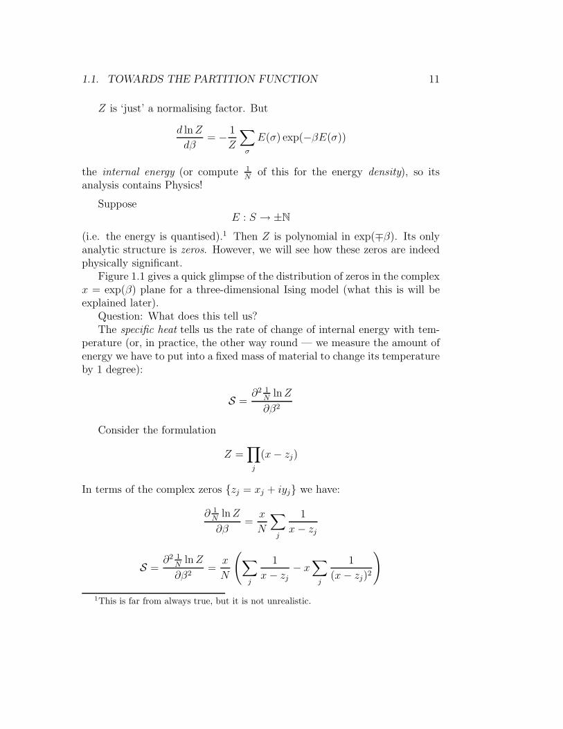
Figure 1.1 gives a quick glimpse of the distribution of zeros in the complexx = exp(β) plane for a three-dimensional Ising model (what this is will beexplained later).

Question: What does this tell us?The specific heat tells us the rate of change of internal energy with tem-

perature (or, in practice, the other way round — we measure the amount ofenergy we have to put into a fixed mass of material to change its temperatureby 1 degree):

S =∂2 1

Nln Z

∂β2

Consider the formulation

Z =∏

j

(x − zj)

In terms of the complex zeros {zj = xj + iyj} we have:

∂ 1N

lnZ

∂β=

x

N

∑

j

1

x − zj

S =∂2 1

Nln Z

∂β2=

x

N

(∑

j

1

x − zj

− x∑

j

1

(x − zj)2

)

1This is far from always true, but it is not unrealistic.


zeros of Z

Figure 1.1: Complex zeros of the partition function for a cubical lattice Isingmodel of about N = 150 sites [11, 15].


Note that the complex zeros appear in conjugate pairs. Performing the sumwithin each conjugate pair this becomes

S =2x

N

(′∑

j

x − xj

(x − xj)2 + y2j

− x

′∑

j

(x − xj)2 − y2

j

((x − xj)2 − y2j )

2 + 4(x − xj)2y2j

)

Consider the contribution of the j-th term (i.e. from a pair of zeros) to S,at some point on the real x axis. Note that if yj is large, or if x− xj is large,then this contribution is small. Meanwhile the contribution is large if thezeros are close to the axis, and x is close to these zeros. In particular thecontribution is large if x = xj , whereupon

Sj ∼2x2

Ny2j

Simply put, this says that, moving along the real line (real temperature),S and U go crazy when there are complex zeros close by (as there are at aparticular point in Figure 1.1, for example).Accordingly we shall call a region of the complex plane that is close to thereal axis and contains zeros of Z a critical neighbourhood of Z.

Let us (very crudely) compare with physical observation.When we boil a kettle we put roughly equal amount of energy into the waterin each unit of time. At first the temperature rises, and the rate of rise doesnot change very much as the temperature goes up. That is, the specific heatchanges slowly and smoothly with temperature. Close to and at the boilingpoint, however, the temperature rise essentially stops, i.e. the amount ofenergy required to further change the temperature becomes very large. Inthe practical experiment there are a number of reasons for this, but one ofthem is that the specific heat becomes very large. Thus we associate divergentspecific heat with a phase transition (in this case the liquid-gas transition atthe boiling point).

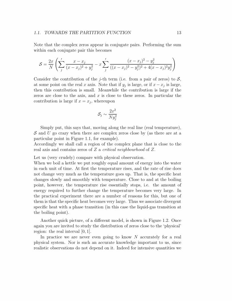
Another quick picture, of a different model, is shown in Figure 1.2. Onceagain you are invited to study the distribution of zeros close to the ‘physical’region: the real interval [0, 1].

In practice we are never even going to know N accurately for a realphysical system. Nor is such an accurate knowledge important to us, sincerealistic observations do not depend on it. Indeed for intensive quantities we


+

+

+

+

+

+

+

+

+

+

+

+

+

+

+

+

+

+

+

+

+

+

+

+

+

+

+

+

+

+

+

+

+

+

+

+

+

+

+

+

+

+

+

+

+

+

+

+

+

+

+

+

+

+

+

+

+

+

+

+

+

+

+

+

+

+

+

+

+

+

+

+

+

+

+

+

+

+

+

+

+

+

+

+

+

+

+

+

+

+

+

+

+

+

+

+

+

+

+

+

+

+

+

+

+

+

+

+

+

+

+

+

+

+

+

+

+

+

+

+

+

+

+

+

+

+

+

+

+

+

+

+

+

+

+

+

+

+

+

+

+

+

+

+

+

+

+

+

+

+

+

+

+

+

+

+

+

+

+

+

+

+

+

+

+

+

+

+

+

+

+

+

+

+

+

+

+

+

+

+

+

+

+

+

+

+

+

+

+

+

+

+

+

+

+

+

+

+

+

+

+

+

+

+

+

+

+

+

+

+

+

+

+

+

+

+

+

+

++

+

+

+

+

+

+

+

+

+

+

+

+

+

+

+

+

+

+

+

+

+

+

+

+

+

+

+

+

+

+

+

+

+

+

+

+

+

+

+

+

+

+

+

+

+

+

+

+

++

+

+

+

+

+

+

+

+

+

+

+

+

+

+

+

+

+

+

+

+

+

+

+

+

+

+

+

+

+

+

+

+

+

+

+

+

+

+

+

+

+

+

+

+

+

+

+

+

+

+

+

+

+

+

+

+

+

+

+

+

+

+

+

+

+

+

+

+

+

+

+

+

+

+

+

+

+

+

+

+

+

+

+

+

+

+

+

+

+

+

+

+

+

+

+

+

+

+

+

+

+

+

+

+

+

+

+

+

+

+

+

+

+

+

+

+

+

+

++

+

+

+

+

+

+

+

+

+

+

+

+

+

+

+

+

+

+

+

+

+

+

+

+

+

+

+

+

+

+

+

+

+

+

+

+

+

+

+

+

+

+

+

+

+

+

+

+

+

+

+

+

+

+

+

+

+

+

+

+

+

+

+

+

+

+

+

+

+

+

+

+

+

+

+

+

+

+

+

+

+

+

+

+

+

+

+

+

+

+

+

+

+

+

+

+

+

+

+

+

+

+

+

+

+

+

+

+

+

+

+

+

+

+

+

+

+

+

+

+

+

+

+

+

+

+

+

+

+

+

+

+

+

+

+

+

+

+

+

+

+

+

+

+

+

+

+

+

+

+

+

+

+

+

+

+

+

+

+

+

+

+

+

+

+

+

+

+

+

+

+

+

+

+

+

++

+

+

+

+

+

+

+

+

+

+

+

+

+

+

+

+

+

+

+

+

+

+

+

+

+

+

+

+

+

+

+

+

+

r

r

r

r

r

r

r

r

r

r

r

r

r

r

r

r

r

r

r

r

r

r

r

r

r

r

r

r

r

r

r

r

r

r

r

r

r

r

r

r

r

r

r

r

r

r

r

r

r

r

r

r

r

r

r

r

r

r

r

r

r

r

r

r

r

r

r

r

r

r

r

r

r

r

r

r

r

r

r

r

r

r

r

r

r

r

r

r

r

r

r

r

r

r

r

r

r

r

r

r

r

r

r

r

r

r

r

r

r

r

r

r

r

r

r

r

r

r

r

r

r

r

r

r

r

r

r

r

r

r

r

r

r

r

r

r

r

r

r

r

r

r

r

r

r

r

r

r

r

r

r

r

r

r

r

r

r

r

r

r

r

r

r

r

r

r

r

r

r

r

r

r

r

r

r

r

r

r

r

r

r

r

r

r

r

r

r

r

r

r

r

r

r

r

r

r

r

r

r

r

r

r

r

r

r

r

r

r

r

r

r

r

r

r

r

r

r

r

r

r

r

r

r

r

r

r

r

r

r

r

r

r

r

r

r

r

r

r

r

r

r

r

r

r

r

r

r

r

r

r

r

r

r

r

r

r

r

r

r

r

r

r

r

r

r

r

r

r

r

r

r

r

r

r

r

r

r

r

r

r

r

r

r

r

r

r

r

r

r

r

r

r

r

r

r

r

r

r

r

r

r

r

r

r

r

r

r

r

r

r

r

r

r

r

r

r

r

r

r

r

r

r

r

r

r

r

r

r

r

r

r

r

r

r

r

r

r

r

r

r

r

r

r

r

r

r

r

r

r

r

r

r

r

r

r

r

r

r

r

r

r

r

r

r

r

r

r

r

r

r

r

r

r

r

r

r

r

r

r

r

r

r

r

r

r

r

r

r

r

r

r

r

r

r

r

r

r

r

r

r

r

r

r

r

r

r

rr

r

r

r

r

r

r

r

r

r

r

r

r

r

r

r

r

r

r

r

r

r

r

r

r

r

r

r

r

r

r

r

r

r

r

r

r

r

r

r

r

r

r

r

r

r

r

r

r

r

r

r

r

r

r

r

r

r

r

r

r

r

r

r

r

r

r

r

r

r

r

r

r

r

r

r

r

r

r

r

r

r

r

r

r

r

r

r

r

r

r

r

r

r

r

r

r

r

r

r

r

r

r

r

r

r

r

r

r

r

r

r

r

r

r

r

r

r

r

r

r

r

r

r

r

r

r

r

r

r

r

r

r

r

r

r

r

r

r

r

r

r

r

r

r

r

r

r

r

r

r

r

r

r

r

r

r

r

r

r

r

r

r

r

r

r

r

r

r

r

r

r

r

r

r

r

r

r

rr

r

r

r

r

r

r

r

r

r

r

r

r

r

r

r

r

r

r

r

r

r

r

r

r

r

r

r

r

r

r

r

r

r

r

r

r

r

r

r

r

r

r

r

r

r

r

r

r

r

r

r

r

r

r

r

r

r

r

r

r

r

r

r

r

r

r

r

r

r

r

r

r

r

r

r

r

r

r

r

r

r

r

r

r

r

r

r

r

r

r

r

r

r

r

r

r

r

r

r

r

r

r

r

r

r

r

r

r

r

r

r

r

r

r

r

r

r

r

r

r

r

r

r

r

r

r

r

r

r

r

r

r

r

r

r

r

r

r

r

r

rr

r

r

r

r

r

r

r

r

r

r

r

r

r

r

r

r

r

r

r

r

r

Figure 1.2: Complex zeros of the partition function for a two-dimensionalclock model at two different lattice sizes [10].

1.2. MODELS 15

expect them to be stable under even large changes in N , so long as N is largeenough. Thus intensive observations in our model also need to be large Nstable. 2

Our pictures give a clue as to the sense in which this can happen:Different polynomials (different N ; different but suitably ‘similar’ physicalsystems) could have similar distributions, real accumulation points, etc.; andhence manifest behaviour on the physical line in similar ways.Can we at least have a model for this?

1.2 Models

We now briefly introduce a simple choice for E (the microstate energy func-tion), from a Physics perpective.

As noted in Section 1.1.3, to introduce a choice for E for physical mod-elling, we must actually introduce one for each of a whole collection of ‘simi-lar’ systems, and then check the stability of observables across this collection.Mathematically, it is convenient to introduce an E for each of a rather largecollection of (nominally but not necessarily adequately similar) systems, thenrefine this collection by physical considerations post hoc. (We will make allthis very precise later.) This is called choosing a ‘model’. The choice weshall describe here is called the Potts model.

(1.2.1) Some statistical mechanics nomenclature: While kinetic-energy-only(non-interacting) models are rather simple, models in which only the poten-tial energy is accounted for in the microstate energy are much richer (partlybecause aspects of the kinetic energy of the system are encoded in β anyway).Excluding kinetic energy from E means that we are essentially treating ourparticle positions as fixed (that is, not translating). Instead system dynam-ics is manifested in other ways. For example we can consider non-pointlikeparticles, hence with the possibility of magnetic dipole moments. Systemdynamics in this case can be manifested in variations in magnetic dipole ori-entation. In such a setting, particles are called spins. Also, the microstateenergy function is called the Hamiltonian (and typically written H not E).

(1.2.2) Let Γ be the set of graphs. For G ∈ Γ let VG be the vertex set of G(sometimes we will simply write G for VG), and EG the edge set. We adopt

2Note that we do not require a large N limit per se for Physics. But stability and theexistence of such a limit amount to the same thing computationally.


the notationn = {1, 2, ..., n}

For any set S (such as a set of graph vertices) and Q ∈ N write

QS = Hom(S, Q)

for the set of maps from S to Q — each map f asigns a state in q ∈{1, 2, ..., Q} to each vertex s by f(s) = q.

1.2.1 Potts and ZQ-symmetric lattice models

(1.2.3) For Q ∈ N, a Q-state graph Hamiltonian is a map asigning to eachgraph G a map HG in Hom(QVG , Z), or more generally Hom(QVG , R). Wesay that this map HG gives the ‘energy’ of state σ ∈ QVG .

(1.2.4) The idea of a model like this (modelling Physics in some given phys-ical space E) is as follows.(i) one considers a subset of graphs, such that each graph G considered rep-resents (in principle) a given physical system — a collection of degrees offreedom embedded in E.(ii) in particular the degrees of freedom of the system reside on the verticesof G, and each takes values from a range represented by {1, 2, ..., Q}; and(iii) the geometrical relationship of the degrees of freedom is encoded (some-how) in the edges between the vertices.In other words, the set of microstate variables is VG (which does not dependon the edges of G), but the interactions HG between spins will depend onthe edges EG.

(1.2.5) Fixing Q (e.g. Q = 2) we have, for example,

HPottsG (σ) =

∑

(v,v′)∈EG

δσ(v),σ(v′ ) =∑

(v,v′)∈EG

δσ(v)−σ(v′ ),0 (1.4)

HClockG (σ) =

∑

(v,v′)∈EG

cos(2π(σ(v) − σ(v′))/Q) (1.5)

Note that each of these indeed gives a Hamiltonian for each choice of G.However not every G makes sense physically. Here the idea is specifically thatVG represents the set of molecules on some crystal lattice; and EG determinesnearest neighbour molecules on the lattice. For example, see Figure 1.3.

1.2. MODELS 17

or or

3d metal 2d metal more exotic 2-manifold

Figure 1.3:

Such an embedding implies further useful structural properties, as weshall see shortly. We may write G to emphasise the extra structure on G,when it is of such a form.

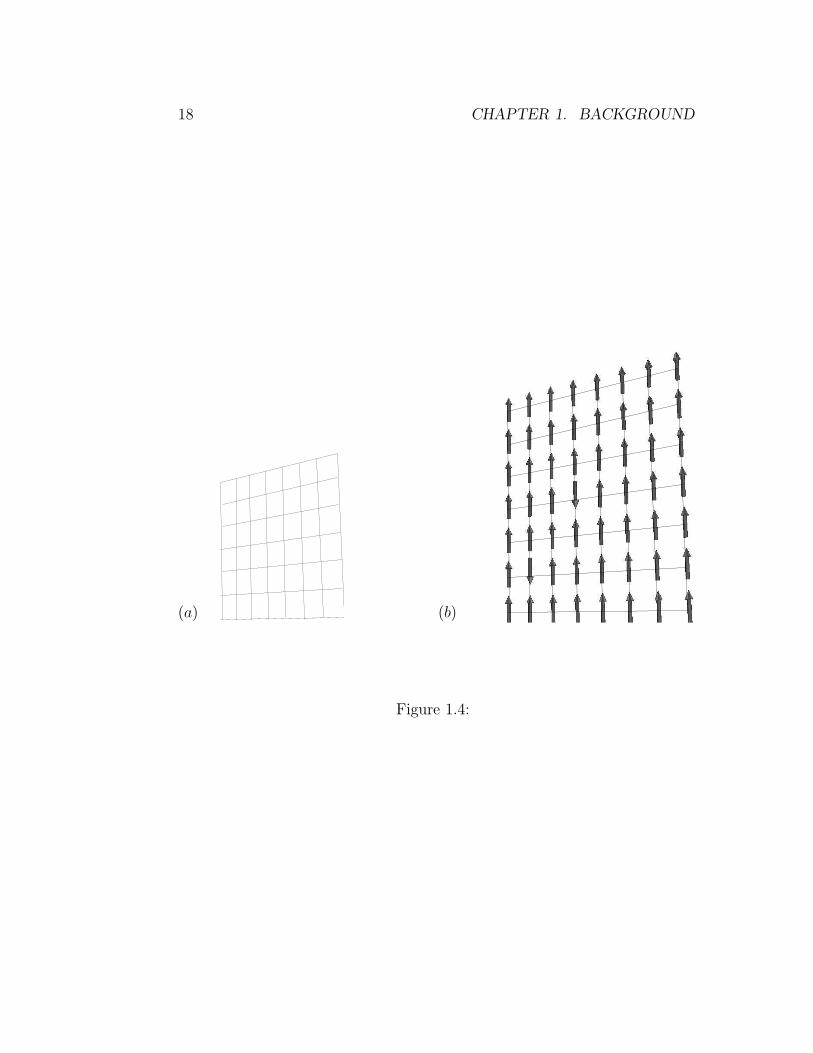
(1.2.6) The 2d square lattice shown, for example, would be part of a sequenceof graphs including also larger square lattices such as the one with 56 verticesand 97 edges shown in Figure 1.4(a).

(1.2.7) Figure 1.4(b) is an example of a Q = 2-state spin configuration onthe vertices of the same square lattice. We draw an up-arrow for the spinstate 1, and a down-arrow for the spin state 2. In this case there are onlytwo down-arrows out of N = 56. Thus HG(σ) = 97 − 8 = 89.


(a) (b)

Figure 1.4:

Chapter 2

More on lattice models

Here we look in a little more detail at certain aspects of the ‘lattice models’introduced in §1.2.1. This Chapter can be skipped at first reading.

2.1 Geometrical aspects

2.1.1 The dual lattice

Note that an embedded graph of the kind discussed in Section 1.2.1 maybe equipped with the structure of a cell complex (see for example Hiltonand Wylie [7, §2.12], Spanier [13, Ch.4]). That is, (I) the embedded graphG defines sets sc(G) of simplices (oriented convex polytopes) of dimensionsc = 0, 1, ..., d, sometimes called c-cells.(II) For each dimension c one also considers the free Z-module with basissc(G), the elements of which are called c-chains. The boundary operator ∂ isa Z-linear map

∂ : Zsc(G) → Zsc−1(G);

for each c, such that ∂2 = 0.For example, if e1 = (v1, v2) is a directed edge of G then ∂e1 = v2 − v1

(we also identify −e1 = (v2, v1)).

(2.1.1) In particular G partitions the d-dimensional embedding space E intopoints, arcs, plaquettes and so on.

We write |G| for the union of all convex cells in the cell complex of G.Strictly speaking, if it is non-empty we include the complement of |G| in E

among the d-cells associated to G.

19

20 CHAPTER 2. MORE ON LATTICE MODELS

(2.1.2) From this perspective the Potts spin configurations are ZQ-valued 0-cochains (regarding ZQ = Z/QZ as an additive group). That is, a c-cochainis a linear map

σ : Zsc(G) → ZQ

for any c, determined by the images of the c-cells. (And the images of thevertices are their values in the Potts spin configuration σ.)

The set of c-cochains form an abelian group by pointwise addition (not avery natural operation from the physical perspective, but a useful organisa-tional device).

(2.1.3) We define a scalar product on cells by (S, S ′) = δS,S′ and extendbi-linearly to chains. This leads to a coboundary operator ∂∗ : Zsc → Zsc+1

by:(S, ∂∗S ′) = (∂S, S ′)

for S ∈ sc, S ′ ∈ sc−1. Note (∂∗)2 = 0.Consider Figure 1.4(a) for example. Let f1 be the face in the top left-

hand corner, and compute ∂∗f1. We have (S, ∂∗f1) = (∂S, f1) = 0 (f1 is notin the boundary of any cell). Thus ∂∗f1 = 0.Meanwhule, let e1 be the edge in the top left-hand corner. We have (S, ∂∗e1) =(∂S, e1) = δS,f1

(up to choice of orientation), thus ∂∗e1 = f1.We can look for a proper subset of chains that forms a ∂∗ subcomplex.

Such a subset can be generated by making a choice of 0-cells to include. Forexample, if we include all the interior 0-cells (in the obvious sense) then allthe interior 1-cells and all the 2-cells must be included, but we do not needto include any of the exterior 0-cells or 1-cells.

(2.1.4) From this structure we may define a Kramers-Wannier dual graphto G. This is a graph (with associated cell complex) D(G) with a vertex vfor each d-dimensional component of G (i.e. a 0-cell for each d-cell), and anedge between v and v′ if their d-dimensional preimages in G share a common(d − 1)-dimensional component (hence a 1-cell for each (d − 1)-cell). Indeed

D : sc(G) → sd−c(D(G))

is a bijection for each c.For example, the dual of our square lattice graph above is shown in Fig-

ure 2.1.

(2.1.5) A c-cochain σ defines a dual (d− c)-cochain D(σ) on sd−c(D(G)) via

D(σ)(D(S)) := σ(S)

2.1. GEOMETRICAL ASPECTS 21

Figure 2.1: Dual lattice of a certain square lattice. All of the exterior verticesare to be identified as the same vertex.

2.1.2 Domain walls

(2.1.6) This dual graph D(G) gives us an alternative way to describe spinconfigurations — in terms of islands of aligned spins, or specifically in termsof the positions of the boundaries of islands of aligned spins. Consider thesquare lattice case, and note that each (directed) edge of the dual graph isassociated to a pair of (ordered) spins, i, j, say, on the original graph. Thenfor a given configuration σ we can asign a directed weight

wij(σ) = σ(j) − σ(i)

(modulo Q) to this dual edge. (We shall orient the dual edges so that, passingfrom i to j, the positive direction of the dual edge across the edge i − j isfrom left to right. We asign w as above to this direction.) In particular, iftwo adjacent spins have the same value in σ then the dual edge weight is zero(and no energy is ‘lost’ at this edge).

For Q odd, a simple notation is to use the representatives of Z/QZ in theinterval [−Q/2, ..., Q/2] for w, and draw w positive-direction pointing arrowson the dual edge if w ≥ 0, or −w reverse arrows if w < 0. The same notationworks for Q even, but note that −Q/2 ≡ Q/2. In the Q = 2 case every dualedge has weight either 1 or 0, for example.


The weight ‘variables’ are Z/QZ-valued, but it is not appropriate to re-place the sum over 0-cochains on the original lattice by the sum over arbitrary1-cochains on the dual lattice, since the map w is not surjective. (It is alsonot injective, but it is made so if we pick and fix any one spin.) The con-straint is that if we traverse a loop around any dual vertex, starting at somespin, then the sum of weights must be congruent to 0 mod. Q (else we donot have a consistent value for the starting spin).

(2.1.7) Note that for Q = 2 the sum of dual edge weights for edges incidentat a give dual vertex, must be even. In general, the sum (taking care of signs,note) must be congruent to zero modulo Q. For Q = 2 that is to say, we canform sequences of dual edges with weight 1 into closed loops. This cannotnecessarily be done uniquely (for example if four weight-1 edges are incidentat a dual vertex), but all equivalent loop asignments correspond to the samespin configuration (up to a global up-down choice).

This means that we can replace the sum over spin configurations by asum over ‘edge coverings’. Coverings are weight asignments to the edges ofthe dual lattice satisfying the covering rule: only asignments with the signedsum of weights incident at each dual vertex congruent to 0 modulo Q areallowed. Every such weight asignment determines a spin configuration, givenonly the state of a single spin. (Note that this ambiguity can be resolvedfreely, since the Hamiltonian (1.4) is invariant under changes in this choice.That is

∑

spin configs

exp(βH) = Q∑

allowedcoverings γ

exp(βH)

Note also that the Hamiltonian can be expressed simply in terms of the totallength of weight-1 boundary in the covering:

H(γ) = |EV | − l(γ) (2.1)

where l(γ) is the length of boundary in covering γ.)

For example, the picture of our spin configuration (b) above is the left-hand picture in Figure 2.2. And here H = |EV | − 8. The right-hand picturein Figure 2.2 shows a different spin configuration and its boundary represen-tation.

This representation of spin configurations is sometimes called the domain

wall representation (for reasons that the figure makes clear).

2.1. GEOMETRICAL ASPECTS 23

Figure 2.2: Two spin configurations with corresponding coverings.

(2.1.8) Note that the covering rule may appear to be modified if one considersonly part of a system, or a system with boundary. Then the details of theconnection with the exterior may be encoded in sinks and sources — dualsites where the incident weight sum is not congruent to 0. See later.

2.1.3 Trivial examples

Consider the lattice consisting of a single square. The dual lattice consistsof two vertices, connected by four edges.

2.1.4 High and low temperature

2.1.5 Kramers–Wannier duality

2.1.6 Graphs with boundary

blah blah!!!


2.A Appendix: Combinatorics of the Potts

groundstate

I have removed the appendix from this point, because it does not belong inan introductory text, and it is not finished. See SM-CombinPotts-1.tex.

Chapter 3

Computation

3.1 Transfer matrix formalism

3.1.1 Partition vectors

Suppose that we have fixed a graph Hamiltonian as in (1.2.3). Then for eachgraph G we have a partition function ZG, associated to the Hamiltonian HG.

(3.1.1) Let ZGV |x

be ZG but with vertex subset V fixed to x:

ZGV |x =

∑

s s.t. state s|V =x

exp(−βH)

Then the ‘Partition vector’ ZGV is a vector indexed by configurations of V ,

whose x-th entry, (ZGV )x, is ZG

V |x.

(3.1.2) If G = G′∪G′′ where VG′ ∩VG′′ = V , EG′ ∩EG′′ = ∅, and HG is ‘local’in the sense that interactions are associated to pairs of vertices defined byedges, then the subgraph partition vector ZG′

V makes sense, and we have

ZG =∑

x

(ZG′

V )x(ZG′′

V )x (3.1)

Typically G has topological properties (perhaps embedded in and rep-resenting some manifold), with respect to which V is a boundary, and thesituation of equation(3.1) may be illustrated as in Figure 3.1 or 3.2.

25

3.1. TRANSFER MATRIX FORMALISM 27

1 2

Figure 3.3: 1. Adding a lattice layer; 2. New larger lattice.

3.1.2 Transfer matrices

Figure 3.2 also server, formally, to define the transfer matrix T = ZTV,V ′ , as a

partition vector with two parts to the ‘boundary’ (note that this is simply anorganisational arrangement). Suppose we iterate composition of a suitableT , as illustrated in Figure 3.3. Then we get

Zbig = 〈T n〉(for suitable initial and final boundary conditions 〈−〉). If {λi}i are theeigenvalues of T we have

Zbig = 〈T n〉 =∑

i

kiλni

where the kis depend on the boundary conditions, but not n. For examplewith simple periodic b.c.s we have

〈T n〉 = Tr(T n) =∑

i

λni

Note that here T is +ve symmetric, so the Perron–Frobenius Theoremimplies

Zbig ∼ k0λn0

(

1 +k1

k0(λ1

λ0)n +

∑

i>1

ki

k0(λi

λ0)n

)

∼ k0λn0

where λ0 is the largest eigenvalue, unless λ1 → λ0 as size→ ∞. So theHelmholtz free energy 1

Nln(Z) ∼ ln(λ0).

What about the physical role of other eigenvalues?


3.1.3 Correlation functions

Cold systems tend to be ordered, and hot systems disordered. Neither ofthese states exhibits long range correlation between local states. Thus onlyin the order/disorder transition region may there be such correlations. Ex-perimentally, correlation of spins over long distance is indeed a signal of phasetransition.

• Experimentally, at a fixed T away from Tc, an observation of the cor-relation of the state of two spins (say) as a function of their separationr, behaves like:

〈σiσi+r〉 ∼ e−r/ρ

(length scale ρ(T ) measured in terms of lattice spacing).

As T → Tc, ρ → ∞ (crucial in lattice Field Theory).

• In Stat Mech

〈σiσi+r〉 ∼(T N1σT rσT N2).

(T N1+r+N2).∼(

λσ

λ0

)r

= exp(−r (ln(λ0) − ln(λσ))︸︷︷︸

1

ρ

)

• So other eigenvalues besides λ0 have physical significance. (NB labelledby operator content, not N , should not depend on N in limit.)

3.2 Practical calculation

3.2.1 Use the force: transfer matrix algebras

Next idea: We look for an algebra A and a representation R such that we canexpress

T = R(X)

with X ∈ A; then organise the spectrum of T by simple components of R.

There is no simple recipe for finding A,R,X to make this work. We shalldiscuss a limited systematisation as we go.

3.2. PRACTICAL CALCULATION 29

1 2 3T = T 1.. . . T = T 1.T 2.. . . T = T 1.T 2.T 3.. . .

4 5 6T = T 1.T 2.T 3.T 4.. . . T = T 1.T 2.T 3.T 4.T 12.. . . T = T 1.T 2.T 3.T 4.T 12.T 23.. . .

Figure 3.4: Growing a cylindrical lattice layer one interaction at a time

Local transfer matrix

The transfer matrix method (essentially requiring that the lattice can made up ofa number of layers) grows the lattice a single layer at a time. Now we go further,and grow the lattice a single interaction at a time.

Let us picture the situation in which we have built some number of completelayers, and now proceed to start building a new layer. We start by adding a singlenew edge/interaction: see Figure 3.4(1). Proceeding as illustrated, here we get

T =∏

i

T i∏

〈i,j〉

T ij (3.2)

What is T i here?

Consider the following example. Take H = −β∑

〈ij〉 δσi,σj (2-state case, say) ona graph made up of closed chain layers (hence a cylindrical lattice, as it were),as in our recent figures. Set x = eβ . Consider the partition vector ZG

W for someassembly of complete layers of lattice G, relative to some collection of ‘boundary’spins W (as in (3.1.1)). One natural arrangement is to take W to be the union ofthe states in some initial layer (on the left) and the states in the most recent layer


grown (on the right) — in which case the partition vector is the transfer matrixT n for some n. Alternatively one might consider Z relative only to the states, Vsay, in the most recently grown layer — i.e. as 〈T n. But consider (for a moment)the partition vector relative to a single spin i in V , preparatory to adding a singlenew interaction involving that spin, as indicated:

i

Zσi=

(Zσi=1

Zσi=2

)

Now consider |V | = m so ZV is a Qm-component vector

ZV =

(

ZV |σi=1

ZV |σi=2

)

where each entry is a Qm−1-component vector. The partition vector for the newsystem, over the new spin, after the new edge is added, is:

Z+σi

=

(xZσi=1 + Zσi=2

Zσi=1 + xZσi=2

)

=

(x 11 x

)

︸︷︷︸

T i=(x−1)IQ+DQ

Zσi

Thus the prefactor matrix on the right is the local transfer matrix.

What is T ij?

Similarly

Z ]σiσj

=

xZ11

Z12

Z21

xZ22

=

x1

1x

︸︷︷︸

T ij=IQ2+(x−1)CQ

Zσiσj

Let us define

ui :=1√Q

IQ ⊗ .. ⊗ DQ︸︷︷︸

i−th

⊗IQ ⊗ .. ⊗ IQ

uij :=√

QIQ ⊗ .. ⊗ CQ︸︷︷︸

i−th and j−th

⊗IQ ⊗ .. ⊗ IQ

3.2. PRACTICAL CALCULATION 31

NB, these obey

u2i =

√

Qui u2ij =

√

Quij uiuijui = ui uijuiuij = uij (3.3)

[ui, uj ] = [uij, ukl] = [ui, ukl] = 0 {i} ∩ {k, l} = ∅ (3.4)

Algebra

• As abstract relations (3.3-3.4) define Graph TL algebra (GTLA) for thecomplete graph Km. A sort of TL version of a Coxeter–Artin group1.

• GTLA for graph G is subalgebra with generators ui and uij if (i, j) ∈ G.

This is generally not finite rank2 but G = Am case is ∼= ordinary TL algebra.

• Thus in 2d

T = R

∏

i

((x − 1)√

Q1 + ui)

∏

ij

(1 +(x − 1)√

Quij)

where R is a representation of OTLA.

• Thus spectrum of T decomposes by irreducible components of R. Thus cor-relation functions (particles) at least partially indexed by simples of algebra.

• This is the paradigm.

Global limit

• Even fixing the physical model, there is a T , and hence a TMA, for each N .

• But physical observables, and hence spectrum components, defined essen-tially independently of N . For given N , spectrum components are (partly)indexed by simple module decomposition of

T = R(X)

, thus these can be indexed independently of N .

• Thus expect global limit to sequence of algebras, and localisation functorspicking out fibres of “physically equivalent” modules.

• How change system size? Example:

Freeze two spins together in transfer matrix layer.

What does this look like at the level of algebra?

1(for Coxeter–Artin groups see (Ram’s translation of) Brieskorn-Saito)2quite interesting. See Martin-Saleur 93


The partition algebra and the Brauer algebra

For Q-state models the overarching algebra is the partition algebra. The partitionalgebra Pn has a basis of partitions of 2 rows of n vertices.

• Pn gives a representation of GTLA.

• consider also the Brauer subalgebra (pair partitions).

3.3 Analysis of results I: generalities and very

low rank

We have seen quite generally that in the physical temperature region the limit freeenergy density is ln λ0 where λ0 is the largest magnitude eigenvalue of the transfermatrix. What becomes of this when we look in the complex x = exp(β) plane, andin particular in our ‘critical’ neighbourhood of the physical region? (As defined inSection 1.1.3.)

To get a bit more out of the 1d Ising model here consider other boundaryconditions. For example, for the AN graph but with end spin states fixed

Z ′(AN ) =(

1 0)(

x 11 x

)(10

)

=1

2(λN

1 + λN2 )

while

Z(AN ) = Tr

(x 11 x

)N

= λN1 + λN

2 = (x + 1)N + (x − 1)N

There are a number of ways that we can recast this simple expression to help thinkabout what might happen in general for large N .

Firstly, we can rewrite

(x + 1)N + (x − 1)N = (x − 1)N ((x + 1

x − 1)N + 1)

Ignoring the first factor we have

Z ∼ Y N + 1 = Y N/2(Y N/2 + Y −N/2)

(where Y = x+1x−1), that is, the remaining zeros are distributed evenly around a

circle. It is the same circle for any N , but the line density increases with N .Setting Y = exp(β′)

f =1

Nln Z =

1

N(ln(2) +

N

2ln Y + ln(cosh(

N

2β′)))

3.3. ANALYSIS OF RESULTS I: GENERALITIES AND VERY LOW RANK33

so

U = −∂ 1N ln Z

∂β′= −1 − tanh(

N

2β′)

That is, the internal energy changes fast (at β′ = 0) for large N .

As we have already seen, the physics is dominated by the zeros close to thereal line, so we can approximate

limN→∞

f ∼ β′/2 +1

2π

∫ ∞

−∞a(y) ln(β′ + iy)dy

where a(y) = 1 (in our case) is the line density of zeros. Thus

U ∼ 1

2πi

∫ ∞

−∞

a(y)dy

y − iβ′

The integrand has a simple pole at y = iβ, so the integral changes by 2πa(0) as β′

changes sign. In other words, if the limit line density a(0) 6= 0 the internal energychanges discontinuously at this point — a first order phase transition.

In practice, in more complicated systems, we can get

a(y) ∼ |y|1−p (0 ≤ p ≤ 1)

but we will return to this shortly.

Notice in our 2× 2 transfer matrix example that the distribution of zeros cor-responds to the locus of points where the largest eigenvalue is actually degenerate(with the other eigenvalue, regarded as an analytic function of β). In fact a largeclass of models have a transfer matrix reducible to a 2 × 2 polynomial matrix T ′.As before

limN→∞

lnZ

N= lim

N→∞ln(λN

+ + λN− )

∗= ln λ+

where * means on the real axis. What happens to the zeros this time?

Consider the general identity

CN + DN =

N−1

2∏

n=−N−1

2

(C + exp(2πin

N)D) =

N−1

2∏

n=1/2

(C2 + D2 + 2cos(2πn/N)CD)

(the explicit limits are for the case N even — the reader will easily compute theodd case). Using this we can rewrite

limN→∞

ln Z

N= lim

N→∞ln(λN

+ + λN− ) =

1

2π

∫ π

0ln(2(A2 + B) + 2 cos y(A2 − B))dy


where A2 − B = CD = λ+λ− and 2(A2 + B) = C2 + D2 = λ2+ + λ2

−, that is

λ± = A ±√

B

Since T ′ is polynomial, so are A and B, and hence the limit is (the log of) aninfinite product of polynomials. One readily confirms that the zeros of this infiniteproduct are the loci

|λ+| = |λ−|

and the endpoints of these loci (if any) are the points where λ+ = λ−, i.e. at rootsof the polynomial B (if B nonvanishing).

(3.3.1) REMARKS: This analysis is essentially taken from [9, Ch.11].

3.4 The 2D Ising model: exact solution

Recall from §1.2.1 that a lattice is an embedding (i.e. a positional but not orienta-tional fixing) of a set of spins in an underlying physical space (usually in a regulararray). Then a lattice model is a model of the bulk behaviour of such a system ofmany interacting lattice spins, determined by a spin interaction Hamiltonian.

Recall the Potts model Hamiltonian (1.4). The Ising model is the two-statePotts model (up to some trivial Hamiltonian rescalings). It will be convenient touse the equivalent ‘Ising form’ of the Potts Hamiltonian here. Thus we have thecollection of partition functions of form

Z =∑

σ

exp(β∑

ij

(2δσi,σj − 1))

where∑

ij is the sum over pairs of nearest neighbour sites in the lattice. In practiceone focusses on a lattice or collection of lattices determined by the embeddingspace. In 2D this collection of lattices is (at least locally) the n × m square grids,with n,m large.

Our strategy in computing Z is to determine a transfer matrix T (acting onthe space of states of an n-site layer of the lattice), such that Z = 〈T m〉, and thento compute by finding a basis for the state space in which T is diagonal.

Let us briefly recall the partition vector/transfer matrix formalism. Fixingthe local Hamiltonian one has a tensor (vector or matrix) for each graph G andcollection {V1, V2, ..., Vr} of (possibly intersecting) subsets of the set of vertices.The i1, i2, ..., ir entry of the tensor is the partition function for G with the spins inVi fixed in state i. Our pictorial notation for this is to draw the graph, together

3.4. THE 2D ISING MODEL: EXACT SOLUTION 35

with a loop around each vertex set Vi. For example, in Q-state models one has

= 1Q = 1⊗nQ T =

where the last picture is the T appropriate for a layer in a square lattice.In the Ising form the local transfer matrix Ti (from (3.2)) for an n-site wide

lattice is

i

= Ti =

(x x−1

x−1 x

)

i

= x12n + x−1σxi = x(12n + x−2σx

i )

(this means Ti acts non-trivially on the ith factor in the layer configuration space,and acts trivially on all the other n − 1 factors). Note that for any scalar θ

eθσx= cosh θ1 + sinh θσx = cosh θ(1 + tanh θσx)

so if we choose θ so that tanh θ = x−2 we get

Ti =x

cosh(θ)eθσx

i = (cosh(θ) sinh(θ))−1/2eθσxi =

√

2 sinh(2β) eθσxi (3.5)

Meanwhile the local transfer matrix Tij is

= Tij =

xx−1

x−1

x

ij

(acting on the adjacent factors i, j), which can be written

Tij = exp

β

1−1

−11

= exp

(

β

(1

−1

)

⊗(

1−1

))


Bruria Kaufman’s (1949) idea is as follows. One notes that V1 =∏

Ti andV2 =

∏Tij can both be equated to certain spin representations of rotations. (These

are representations on tensor space of dimension 2n.) We can then use an abstractrelation to the eigenvalues of a smaller more manageable representation of thesame rotations — the ordinary rotation matrices of dimension 2n. Recall thatthese are generated by the simple plane rotations

wi i+1(θ) = 1i−1 ⊕(

cos(θ) sin(θ)− sin(θ) cos(θ)

)

⊕ 12d−i−1 (3.6)

where the mixing occurs in the i, i + 1-positions.

To understand the spin representations it is convenient to introduce Cliffordalgebras.

(3.4.1) A set {Γa}a=1,...,2n of 2n × 2n matrices such that Γ2a = 1 and

ΓaΓb + ΓbΓa = 0 (a 6= b)

are said to form a Clifford algebra.

(3.4.2) For example, with σxi the usual Pauli matrix action on tensor space:

Γ•2i−1 :=

i−1∏

j=1

σxj

σzi Γ•

2i :=

i−1∏

j=1

σxj

σyi

obey these relations.

In this case note that

Γ•2iΓ

•2i−1 = σy

i σzi = iσx

i Γ•2i+1Γ

•2i = σx

i σzi+1σ

yi = iσz

i σzi+1

Thus from (3.5) et seq

V1 =∏

i

Ti = κnn∏

i=1

e−iθΓ•

2iΓ•

2i−1 V2 =∏

i

Ti i+1 = eβσznσz

1

n−1∏

i=1

e−iβΓ•

2i+1Γ•

2i

where κ =√

2 sinh(2β), and at the last we have applied periodic boundary condi-tions.

3

3 (3.4.3) Note: (i) If {Γa}a is a Clifford algebra, then so is {SΓaS−1}a for any invertible

matrix S ∈ End(C2n

);(ii) the matrices Γ′

aobtained from the Γ•

as by swapping the roles of σx and σz are a Clifford


(3.4.4) Fixing any Clifford algebra {Γa}a we define

S(wab(θ)) = cosθ

21 − sin

θ

2ΓaΓb = exp(

−1

2θΓaΓb)

Example: One can easily find a Clifford algebra {Γ◦a}a such that

exp(−1

2θΓ◦

1Γ◦2) = exp(

−1

2θiσz

1) =

(e−iθ/2

eiθ/2

)

⊗ 12 ⊗ 12... (3.7)

One can check that these matrices obey

S(wab(θ))ΓaS−1(wab(θ)) = cos θΓa + sin θΓb

and so on. In other words conjugation by S(wab(θ)) enacts the rotation wab(θ) onthe space of Γ-matrices (not to be confused with the space on which the Γ-matricesact).

It follows that conjugation by S(wab(θ))S(wcd(θ′)) realises the rotation wab(θ)wcd(θ

′).From this we have a kind of realisation of the group of rotations in 2n-dimensions.(This is not quite a representation, since it is a double-cover, but this need notconcern us.)

(3.4.5) Note from (3.6) that the spectrum of wab(θ) is eiθ, e−iθ (and possibly some1s). (Indeed any element in SO(3) can be expressed as a simple rotation aboutsome, not in general coordinate, axis; and hence has eigenvalues of the same form.)

Meanwhile, noting (3.7), the spectrum of S(wab(θ)) is ei2(±θ) (2n−1 copies of each).

Further, if w =∏

i waibi(θi) with all the {ai, bi} distinct; and S(w) =

∏

i S(waibi(θi)),

then the 2n eigenvalues of w are {e±iθj}j ; and, since the factors in S(w) commute,the 2n eigenvalue of S(w) are

Spectrum(S(w)) = {e i2

Pnj=1

±θj}. (3.8)

algebra.(iii) arbitrarily permute the numbering of the Γas in any Clifford algebra, and the Cliffordrelations will still be obeyed.(iv) Also if {Γa} is any Clifford algebra then Γ′ = rΓ1 + sΓ2 obeys

ΓaΓ′ + Γ′Γa = Γa(rΓ1 + sΓ2) + (rΓ1 + sΓ2)Γa = r(ΓaΓ1 + Γ1Γa) + s(ΓaΓ2 + Γ2Γa) = 0

for all a > 2, for any r, s; and

(cΓ1 + sΓ2)(sΓ1 − cΓ2) + (sΓ1 − cΓ2)(cΓ1 + sΓ2) = 2(cs − sc) = 0

and so on. Following these calculations one eventually checks that Γ1, Γ2 can be replaced bythe indicated linear combinations, so long as c = cos θ and s = sin θ for some θ. Evidentlyone can compose such transformations, so we have an action of the 2n dimensional rotationgroup transforming between realisations of the Clifford relations.


(Later we shall generalise this correspondence to elements of SO(2n) that areproducts of commuting rotations about arbitrary sets of orthogonal axes, not justthe nominal coordinate axes.)

(3.4.6) In these terms, writing S•(w) for S(w) in the Γ• case, we have

V1 = κnn∏

i=1

S•(w2i 2i−1(2iθ))

V2 = χn−1∏

i=1

S•(w2i+1 2i(2iβ))

where χ is the periodic boundary operator. For a suitable treatment of the bound-ary (not quite simple periodic, but close enough) we have χ = S•(w1 2n(2iβ)).

(3.4.7) The idea now is to replace T = V1V2 with the corresponding product ofrotation matrices W = W1W2. We then find the eigenvalues of this product W .Since every rotation group element can be expressed as a product of commutingrotations (not necessarily respecting the initial axes) these eigenvalues will define aset of rotation angles {θi}i as above. We claim that this set then give the spectrumof T , as in (3.8).

We have (in a representative small example, n = 4), with c = cos(2iθ), s =sin(2iθ), and so on,

W1 = w12(2iθ)w34(2iθ)w56(2iθ)w78(2iθ) =

c s−s c

c s−s c

c s−s c

c s−s c

W2 =

c′ −s′

c′ s′

−s′ c′

c′ s′

−s′ c′

c′ s′

−s′ c′

s′ c′


Note that W1,W2 are both fixed by the square of the matrix position shiftoperator (and that this is true for general n). Accordingly we can fourier transformto block diagonalise W . That is, we make a change of basis as follows. Definefz = (1, z, z2, z3, ..., zn−1)t, vz = (1, 0)t ⊗ fz and v′z = (0, 1)t ⊗ fz. With zn = 1 wehave

W1

(vz

v′z

)

=

(c −ss c

)(vz

v′z

)

W2

(vz

v′z

)

=

(c′ zs′

−z−1s′ c′

)(vz

v′z

)

W

(vz

v′z

)

=

(cc′ + z−1ss′ zcs′ − sc′

sc′ − z−1cs′ cc′ + zss′

)(vz

v′z

)

Noting that the determinant of the image matrix W (z) on the right is 1 we writethe eigenvalues as λ± = e±lz . Thus

elz + e−lz = Trace(W (z)) = 2

(

cc′ +z + z−1

2ss′)

That is,

cosh(lz) =

(

cosh(2θ) cosh(2β) − z + z−1

2sinh(2θ) sinh(2β)

)

Since z is any solution to zn = 1, the complete set of lzs is obtained from z = e2πik/n

with k = 1, .., n. One then finds that each lz is positive for physical parameters.It follows that the largest among the eigenvalues for T that this gives:

λ = exp

(

1

2

n∑

k=1

±le2πik/n

)

is the case

λ0 = exp

(

1

2

n∑

k=1

le2πik/n

)

Recall that this is for an n-site wide lattice. If the lattice is m sites long then

Z ∼ λm0

1 +∑

i6=0

(λi

λ0)m

∼ λm0 ,

or more usefully, the free energy is f = 1nm ln Z ∼ (1/n) ln λ0, with this approxi-

mation getting better as m gets bigger and becoming an equality in the large mlimit.


Now we follow [9, §4.1] for the rest of the analysis. Using that

sinh(2β) = sinh(2θ)−1 and coth(2β) = cosh(2θ)

we have

cosh(lz) =

(

coth(2β) cosh(2β) − z + z−1

2

)

which it is convenient to express via the integral representation4

lz =1

π

∫ π

0dy ln(2(coth(2β) cosh(2β) − z + z−1

2) − 2 cos(y))

giving

ln λ0 =1

2

n∑

k=1

1

π

∫ π

0dy ln(2 coth(2β) cosh(2β) − 2 cos(2πk/n) − 2 cos(y))

Note how the difference in the way we have treated m and n is manifested here.We are looking at the free energy in the infinite-m limit (hence the integral), butwith n still finite. We can rigorously bring the treatment of the two directionsonto the same footing by taking the large n limit (which will covert the sum toa matching integral); or we can roughly discretise the integral to a sum over mterms, using the sum over n terms as a guide:

∫ π

0f(y)dy ∼ π

M

M∑

r=1

f(πr/M)

(any M >> 1).

In the latter case we get (see e.g. [?])

Zmn =

m∏

r=1

n∏

s=1

{

1 − K

2(cos(2πr/m) + cos(2πs/n))

}

where

K = 4exp(−2β)(1 − exp(−4β)))

(1 + exp(−4β))2

4recall cosh−1 x = ln(x +√

x2 − 1) = lnx + ln(1 +√

1 + x−2) and

π ln(1 +√

1 − t2) =

∫π

0

ln(1 + t cosw)dw


T_cTemp

Figure 3.5: Sketch plot of specific heat versus temperature for the 2D Isingmodel.

Note that each factor in Znm is invariant under x → −x, and

1

x2→ tanh β =

eβ − e−β

eβ + e−β= (x2 − 1)/(x2 + 1)

The fixed point of this transformation is given by

−(x2 + 1) + (x2 − 1)x2 = x4 − 2x2 − 1 = (x2 − (−√

2 + 1))(x2 − (√

2 + 1)) = 0

x2 = exp(2β) = 1 +√

2

Note that this also determines the ferromagnetic critical point.A very rough sketch of the second log-derivative (the specific heat) versus

T = 1/β is given in Figure 3.5. The divergence is logarithmic: close to Tc we have

S(T ) ∼ − ln |Tc − T |

Chapter 4

Spin chains

This Chapter is largely unfinished, but for now contains some useful notation.

4.1 Anisotropic limit

Here we consider a ‘continuous time’ approximation to the Ising model. (Here‘time’ is a misnomer for the layering direction in the transfer matrix formalism.)In this case one takes an infinite lattice limit in the layering direction first, butadjusts the couplings anisotropically to compensate. There is then a non-trivialsimplification of the general problem arising. This has the flavour of a quantumHamiltonian limit of the transfer matrix (which will lead conveniently to the laterconsideration of such Hamiltonians per se).

— TO DO! —

4.2 XXZ spin chain

In some formalisms, such as quantum theory, the energy function E (the ‘classicalHamiltonian’) is replaced by an operator on the space of states. In such cases, thefirst mathematical challenge is to determine the eigenvalues and eigenvectors ofthis Hamiltonian operator.

We describe the Heisenberg chain Hamiltonian and a number of variationsthereof. The eigenvalue problem is hard for these systems, for anything other thanvery small chain length. In the absence of a complete solution, Physical interestmay justify trying to solve just for the lowest (respectively highest) eigenvalue, itsdegeneracy, and the gap to the next lowest.

43

44 CHAPTER 4. SPIN CHAINS

4.2.1 Notations and conventions

Define

σx =

(0 11 0

)

iσy =

(0 1−1 0

)

σz =

(1 00 −1

)

so that

σ+ =1

2(σx + iσy) =

(0 10 0

)

Our convention in the Kronecker product A ⊗ B is to order so that

σ+ ⊗ σ− =

0 0 0 00 0 1 00 0 0 00 0 0 0

and σz ⊗ 12 =

1 0 0 00 1 0 00 0 −1 00 0 0 −1

Now fix L and define operators σxi (and so on) on (C2)⊗L so that:

σxi σx

i+1 = 12 ⊗· · ·⊗(

0 11 0

)

⊗(

0 11 0

)

⊗· · · = 12 ⊗· · ·⊗

0 0 0 10 0 1 00 1 0 01 0 0 0

⊗· · ·

σzi σ

zi+1 = 12⊗· · ·⊗

(1 00 −1

)

⊗(

1 00 −1

)

· · · = 12⊗· · ·⊗

1 0 0 00 −1 0 00 0 −1 00 0 0 1

· · ·

4.2.2 Hamiltonia

uXY Zij (kx, ky, kz) :=

1

2(kxσx

i σxj + kyσ

yi σy

j + kzσzi σ

zj )

uXY Zi (kx, ky , kz) := uXY Z

i i+1 (kx, ky, kz)

(by uL we shall intend the periodic closure uL,1)

uXXZi = uXY Z

i (1, 1,−q + q−1

2) =

− δ4 0 0 0

0 δ4 1 0

0 1 δ4 0

0 0 0 − δ4

i

4.2. XXZ SPIN CHAIN 45

where δ = q + q−1 ∈ C; uXXXi = uXY Z

i (1, 1, 1); uXYi = uXY Z

i (1 + a, 1 − a, 0)(a ∈ R);

ui = uXXZi +

1

2

q + q−1

2− 1

2

q − q−1

2(σz

i − σzi+1) =

0 0 0 00 q 1 00 1 q−1 00 0 0 0

The simple periodic Heisenberg chain (without external field) is the Hamiltonian

HXXX = uXXXL +

L−1∑

i=1

uXXXi

Generalisations include

HXXZpp′ :=

L−1∑

i=1

uXXZi + pσz

1 + p′σzL HXXZ :=

∑

i

ui

(see e.g. [?]). We shall be interested in the spectrum of these matrices. The matrixHXXZ differs from a sum of the uXXZ

i by an additive scalar and boundary terms,so both are forms of XXZ spin chain Hamiltonian.

The anisotropic limit Potts model Hamiltonian is (roughly) in the same uni-versality class as the Potts model. It also takes the same form as HXXZ , exceptfor being in a different representation of the TL algebra. For this reason (amongothers) one is interested in the spectrum of HXXZ .

(Potts model unsolved.)

4.2.3 Normal Bethe ansatz

We are interested in the spectrum of H = HXXZpp′ (or specifically HXXZ , or indeed

any similar case).

We take words in {1, 2} of length L as a basis for (C2)L. For any fixed butarbitrary L, let us write vx = v(x1, ..., xJ ) for the vector with 2s in the J indicatedpositions. Clearly the subspaces spanned by vectors with J fixed are invariantunder H, so for each J we may look for eigenvectors w obeying

Hw = Eww

with

w =∑

1≤x1<...<xi<xi+1<...<xJ≤L

cxvx


(We call the excess of 1s over 2s, given by L − 2J , the charge. Whether Physicalinterest resides mainly in low or high charge depends on the details. Here we shallconcetrate on what can be said about eigenvalues in general.)

It will be evident that there is only one vector (hence eigenvector) with J = 0.We have

HXXZ 111...1 = 0

For J = 1 we have

Hv1 = (u1 + u2 + ... + uL−1)v1 = q−1v1 + v2

Hvi = vi−1 + (q + q−1)vi + vi+1 (1 < i < L)

HvL = qvL + vL−1

so thatHw =

∑

j

cjHvj = Ew

∑

j

cjvj

gives the following. Coefficient of v1 (then vi, then vL):

Ec1 = c1q−1 + c2

Eci = ci−1 + ci(q + q−1) + ci+1 (1 < i < L) (4.1)

EcL = cLq + cL−1

All three forms coincide if we use the boundary conditions

c0 = −qc1 cL+1 = −q−1cL

Following Alcaraz et al one tries for a solution of form

cj = A(k)eijk + A(−k)e−ijk

where viable choices for k, and for each k the constant A, are to be determined.Substituting into (4.1) we have

Ek − (q + q−1)(A(k)eijk + A(−k)e−ijk)

= A(k)eijke−ik + A(−k)e−ijkeik + A(k)eijkeik + A(−k)e−ijke−ik

givingEk = (q + q−1) + 2 cos(k)

CHECK THIS!It remains to impose the boundary conditions, which, if they can be satisfied,

will determine the possible values of k. The c0 condition gives

A(0) + A(0) = −q(A(1)eik + A(−1)e−ik)

.1. APPENDIX: WHAT IS PHYSICS? 47

4.2.4 Abstract Bethe ansatz

4.2.5 Gram matrices

Acknowledgements

Thanks to Yogi Valani for many useful discussions.Thanks to my coorganisers of Leeds SMDG, Jeanne Scott and Sathish Sukumaranfor all their considerable efforts to make it work.

.1 Appendix: What is Physics?

Statistical Mechanics is part of Physics. Physics might be characterised, in thelarge, as the scientific exercise (as opposed to involuntary reflex) of modelling ofthe observable physical world. That is, the representation of part of the physicalworld by something ‘simpler’, which nonetheless captures some of the physicalworld’s humanistically essential features.There are various phases to this exercise, such as:(i) deciding which toy is the model;(ii) working out what the model itself does; and(iii) interpreting this behaviour as a prediction for the physical world.

The simple toys at our disposal include real toys (scale models of bridges andso on), and systems of equations in mathematics. 1 In particular Scientists havehad notable success summarizing large amounts of observational data from thephysical world with certain relatively simple mathematical models. A very suc-cessful such model is, reasonably, regarded as close to nature itself; and hencefundamental. Key to this is the expectation that such a model, pushed into an asyet unobserved (but suitably nearby) regime, will correctly predict the result ofobservations subsequently made there. There has been notable success too in thispredictive aspect of Physics, and great technological benefits have accrued.

Bibliography

Some relevant texts are, for Statistical Mechanics: Baxter[2], Domb and Green[3],Levy[8], Martin[9], and Wannier[16];

1Note that these toys either exist themselves in the physical world, or are abstractionsformulated by creatures living in the physical world (and whose thought processes are tiedto making sense of this experience). This is of course unavoidable, but singular. Otherproblems in representation theory are not constrained to have all representations builtinside the thing being represented.


for generalities: Abramowitz and Stegun[1], Feynman[6].

Bibliography

[1] Milton Abramowitz and Irene A. Stegun, Handbook of mathematical functionswith formulas, graphs, and mathematical tables, Dover, New York, 1964.

[2] R J Baxter, Exactly solved models in statistical mechanics, Academic Press,New York, 1982.

[3] C Domb and M S Green (eds.), Phase transitions and critical phenomena I,Academic Press, London, New York, 1972.

[4] M B Einhorn, R Savit, and E Rabinovici, A physical picture for the phasetransition in ZN symmetric models, Nucl Phys B 170 [FS1] (1980), 16.

[5] S Elitzur, R B Pearson, and J Shigemitsu, The phase structure of discreteabelian spin and gauge systems, Phys Rev D 19 (1979), 3698.

[6] Richard P Feynman, The Feynman lectures on physics: Volume 3, Addison-Wesley, Boston, 1963.

[7] P J Hilton and S Wylie, Homology theory, Cambridge, 1965.

[8] R A Levy, Principles of Solid State Physics, Academic Press, New York, 1968.

[9] P P Martin, Potts models and related problems in statistical mechanics, WorldScientific, Singapore, 1991.

[10] P P Martin and A Elgamal, Ramified partition algebras, Math. Z. 246 (2004),473–500, (math.RT/0206148).

[11] P P Martin and Y Valani, Non-integrable Potts models revisited, In prepara-tion (2008).

[12] G Polya and R C Read, Combinatorial enumeration of groups, graphs, andchemical compounds, Springer-Verlag, New York, 1987.

[13] E H Spanier, Algebraic topology, McGraw–Hill, New York, 1966.

49

50 BIBLIOGRAPHY

[14] R M Thompson and R T Downs, Systematic generation of all nonequiva-lent closest-packed stacking sequences of length n using group theory, ActaCrystallographica B57 (2001), 766–771.

[15] Y Valani, Temperature zeros of the Potts model partition function revisited,Ph.D. thesis, City University, In preparation.

[16] G H Wannier, Statistical physics, Wiley, 1966.

an introduction to basic statistical mechanics for ...ppmartin/pdf/sm1-1.pdfso where does...

Documents