an introduction to computational finance without agonizing ... · an introduction to computational...
TRANSCRIPT
An Introduction to Computational FinanceWithout Agonizing Pain
P.A. Forsyth∗
November 20, 2002
Contents
1 The First Option Trade 3
2 The Black-Scholes Equation 32.1 Background . . . . . . . . . . . . . . . . . . . . . . . . . . . . . . . . . . . . 32.2 Definitions . . . . . . . . . . . . . . . . . . . . . . . . . . . . . . . . . . . . . 42.3 A Simple Example: The Two State Tree . . . . . . . . . . . . . . . . . . . . 42.4 A hedging strategy . . . . . . . . . . . . . . . . . . . . . . . . . . . . . . . . 52.5 Brownian Motion . . . . . . . . . . . . . . . . . . . . . . . . . . . . . . . . . 62.6 Geometric Brownian motion with drift . . . . . . . . . . . . . . . . . . . . . 11
2.6.1 Ito’s Lemma . . . . . . . . . . . . . . . . . . . . . . . . . . . . . . . . 122.6.2 Some uses of Ito’s Lemma . . . . . . . . . . . . . . . . . . . . . . . . 13
2.7 The Black-Scholes Analysis . . . . . . . . . . . . . . . . . . . . . . . . . . . 142.8 Hedging in Continuous Time . . . . . . . . . . . . . . . . . . . . . . . . . . . 162.9 The option price . . . . . . . . . . . . . . . . . . . . . . . . . . . . . . . . . 162.10 American early exercise . . . . . . . . . . . . . . . . . . . . . . . . . . . . . . 17
3 The Risk Neutral World 17
4 Monte Carlo Methods 194.1 Monte Carlo Error Estimators . . . . . . . . . . . . . . . . . . . . . . . . . . 224.2 Random Numbers and Monte Carlo . . . . . . . . . . . . . . . . . . . . . . . 224.3 The Box-Muller Algorithm . . . . . . . . . . . . . . . . . . . . . . . . . . . . 24
∗Department of Computer Science, University of Waterloo, Waterloo, Ontario, Canada, N2L 3G1,[email protected], www.scicom.uwaterloo.ca/ paforsyt, tel: (519) 888-4567x4415, fax:(519) 885-1208
1
4.3.1 An improved Box Muller . . . . . . . . . . . . . . . . . . . . . . . . . 254.4 Speeding up Monte Carlo . . . . . . . . . . . . . . . . . . . . . . . . . . . . 284.5 Estimating the mean and variance . . . . . . . . . . . . . . . . . . . . . . . . 294.6 Low Discrepancy Sequences . . . . . . . . . . . . . . . . . . . . . . . . . . . 294.7 Correlated Random Numbers . . . . . . . . . . . . . . . . . . . . . . . . . . 31
5 The Binomial Model 335.1 A No-arbitrage Lattice . . . . . . . . . . . . . . . . . . . . . . . . . . . . . . 355.2 More on Ito’s Lemma . . . . . . . . . . . . . . . . . . . . . . . . . . . . . . . 37
6 Derivative Contracts on non-traded Assets and Real Options 406.1 Derivative Contracts . . . . . . . . . . . . . . . . . . . . . . . . . . . . . . . 406.2 A Forward Contract . . . . . . . . . . . . . . . . . . . . . . . . . . . . . . . 44
6.2.1 Convenience Yield . . . . . . . . . . . . . . . . . . . . . . . . . . . . 45
7 Discrete Hedging 457.1 Delta Hedging . . . . . . . . . . . . . . . . . . . . . . . . . . . . . . . . . . . 457.2 Gamma Hedging . . . . . . . . . . . . . . . . . . . . . . . . . . . . . . . . . 47
8 Jump Diffusion 498.1 The Poisson Process . . . . . . . . . . . . . . . . . . . . . . . . . . . . . . . 508.2 The Jump Diffusion Pricing Equation . . . . . . . . . . . . . . . . . . . . . . 52
9 Further Reading 53
2
“Men wanted for hazardous journey, small wages, bitter cold, long months ofcomplete darkness, constant dangers, safe return doubtful. Honour and recogni-tion in case of success.” Advertisement placed by Earnest Shackleton in 1914.He received 5000 replies. An example of extreme risk-seeking behaviour. Hedg-ing with options is used to mitigate risk, and would not appeal to members ofShackleton’s expedition.
1 The First Option Trade
Many people think that options and futures are recent inventions. However, options have along history, going back to ancient Greece.
As recorded by Aristotle in Politics, the fifth century BC philosopher Thales of Miletustook part in a sophisticated trading strategy. The main point of this trade was to confirmthat philosophers could become rich if they so chose. This is perhaps the first rejoinder tothe famous question “If you are so smart, why aren’t you rich?” which has dogged academicsthroughout the ages.
Thales observed that the weather was very favourable to a good olive crop, which wouldresult in a bumper harvest of olives. If there was an established Athens Board of OlivesExchange, Thales could have simply sold olive futures short (a surplus of olives would causethe price of olives to go down). Since the exchange did not exist, Thales put a deposit onall the olive presses surrounding Miletus. When the olive crop was harvested, demand forolive presses reached enormous proportions (olives were not a storable commodity). Thalesthen sublet the presses for a profit. Note that by placing a deposit on the presses, Thaleswas actually manufacturing an option on the olive crop, i.e. the most he could lose was hisdeposit. If had sold short olive futures, he would have been liable to an unlimited loss, in theevent that the olive crop turned out bad, and the price of olives went up. In other words, hehad an option on a future of a non-storable commodity.
2 The Black-Scholes Equation
This is the basic PDE used in option pricing. We will derive this PDE for a simple casebelow. Things get much more complicated for real contracts.
2.1 Background
Over the past few years derivative securities (options, futures, and forward contracts) havebecome essential tools for corporations and investors alike. Derivatives facilitate the transferof financial risks. As such, they may be used to hedge risk exposures or to assume risks inthe anticipation of profits. To take a simple yet instructive example, a gold mining firm isexposed to fluctuations in the price of gold. The firm could use a forward contract to fix theprice of its future sales. This would protect the firm against a fall in the price of gold, but itwould also sacrifice the upside potential from a gold price increase. This could be preservedby using options instead of a forward contract.
3
Individual investors can also use derivatives as part of their investment strategies. Thiscan be done through direct trading on financial exchanges. In addition, it is quite commonfor financial products to include some form of embedded derivative. Any insurance contractcan be viewed as a put option. Consequently, any investment which provides some kind ofprotection actually includes an option feature. Standard examples include deposit insuranceguarantees on savings accounts as well as the provision of being able to redeem a savings bondat par at any time. These types of embedded options are becoming increasingly commonand increasingly complex. A prominent current example are investment guarantees beingoffered by insurance companies (“segregated funds”) and mutual funds. In such contracts,the initial investment is guaranteed, and gains can be locked-in (reset) a fixed number oftimes per year at the option of the contract holder. This is actually a very complex putoption, known as a shout option. How much should an investor be willing to pay for thisinsurance? Determining the fair market value of these sorts of contracts is a problem inoption pricing.
2.2 Definitions
Let’s consider some simple European put/call options. At some time T in the future (theexpiry or exercise date) the holder has the right, but not the obligation, to
• Buy an asset at a prescribed price K (the exercise or strike price). This is a call option.
• Sell the asset at a prescribed price K (the exercise or strike price). This is a put option.
At expiry time T , we know with certainty what the value of the option is, in terms of theprice of the underlying asset S,
Payoff = max(S −K, 0) for a call
Payoff = max(K − S, 0) for a put (2.1)
Note that the payoff from an option is always non-negative, since the holder has a right butnot an obligation. This contrasts with a forward contract, where the holder must buy or sellat a prescribed price.
2.3 A Simple Example: The Two State Tree
This example is taken from Options, futures, and other derivatives, by John Hull. Supposethe value of a stock is currently $20. It is known that at the end of three months, the stockprice will be either $22 or $18. We assume that the stock pays no dividends, and we wouldlike to value a European call option to buy the stock in three months for $21. This optioncan have only two possible values in three months: if the stock price is $22, the option isworth $1, if the stock price is $18, the option is worth zero. This is illustrated in Figure 1.
In order to price this option, we can set up an imaginary portfolio consisting of the optionand the stock, in such a way that there is no uncertainty about the value of the portfolio atthe end of three months. Since the portfolio has no risk, the return earned by this portfoliomust be the risk-free rate.
4
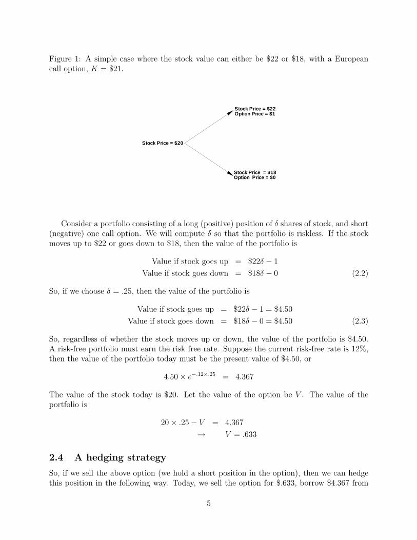
Figure 1: A simple case where the stock value can either be $22 or $18, with a Europeancall option, K = $21.
Stock Price = $20
Stock Price = $22Option Price = $1
Stock Price = $18Option Price = $0
Consider a portfolio consisting of a long (positive) position of δ shares of stock, and short(negative) one call option. We will compute δ so that the portfolio is riskless. If the stockmoves up to $22 or goes down to $18, then the value of the portfolio is
Value if stock goes up = $22δ − 1
Value if stock goes down = $18δ − 0 (2.2)
So, if we choose δ = .25, then the value of the portfolio is
Value if stock goes up = $22δ − 1 = $4.50
Value if stock goes down = $18δ − 0 = $4.50 (2.3)
So, regardless of whether the stock moves up or down, the value of the portfolio is $4.50.A risk-free portfolio must earn the risk free rate. Suppose the current risk-free rate is 12%,then the value of the portfolio today must be the present value of $4.50, or
4.50× e−.12×.25 = 4.367
The value of the stock today is $20. Let the value of the option be V . The value of theportfolio is
20× .25− V = 4.367
→ V = .633
2.4 A hedging strategy
So, if we sell the above option (we hold a short position in the option), then we can hedgethis position in the following way. Today, we sell the option for $.633, borrow $4.367 from
5

the bank at the risk free rate (this means that we have to pay the bank back $4.50 in threemonths), which gives us $5.00 in cash. Then, we buy .25 shares at $20.00 (the current priceof the stock). In three months time, one of two things happens
• The stock goes up to $22, our stock holding is now worth $5.50, we pay the optionholder $1.00, which leaves us with $4.50, just enough to pay off the bank loan.
• The stock goes down to $18.00. The call option is worthless. The value of the stockholding is now $4.50, which is just enough to pay off the bank loan.
Consequently, in this simple situation, we see that the theoretical price of the option is thecost for the seller to set up portfolio, which will precisely pay off the option holder and anybank loans required to set up the hedge, at the expiry of the option. In other words, thisis price which a hedger requires to ensure that there is always just enough money at theend to net out at zero gain or loss. If the market price of the option was higher than thisvalue, the seller could sell at the higher price and lock in an instantaneous risk-free gain.Alternatively, if the market price of the option was lower than the theoretical, or fair marketvalue, it would be possible to lock in a risk-free gain by selling the portfolio short. Anysuch arbitrage opportunities are rapidly exploited in the market, so that for most investors,we can assume that such opportunities are not possible (the no arbitrage condition), andtherefore that the market price of the option should be the theoretical price.
Note that this hedge works regardless of whether or not the stock goes up or down.Once we set up this hedge, we don’t have a care in the world. The value of the option isalso independent of the probability that the stock goes up to $22 or down to $18. This issomewhat counterintuitive.
2.5 Brownian Motion
Before we consider a model for stock price movements, let’s consider the idea of Brownianmotion with drift. Suppose X is a random variable, and in time t→ t + dt, X → X + dX,where
dX = αdt + σdZ (2.4)
where αdt is the drift term, σ is the volatility, and dZ is a random term. The dZ term hasthe form
dZ = φ√dt (2.5)
where φ is a random variable drawn from a normal distribution with mean zero and varianceone (φ is N(0, 1)).
If E is the expectation operator, then
E(φ) = 0 E(φ2) = 1 . (2.6)
Now in a time interval dt, we have
E(dX) = E(αdt) + E(σdZ)
= αdt , (2.7)
6
X0
X0 - ∆h
X0 - 2∆h
X0 + 2∆h
X0 + ∆hp
q
p2
q2
q3
p3
2pq
3p2q
3pq2
X0 + 3∆h
X0 - 3∆h
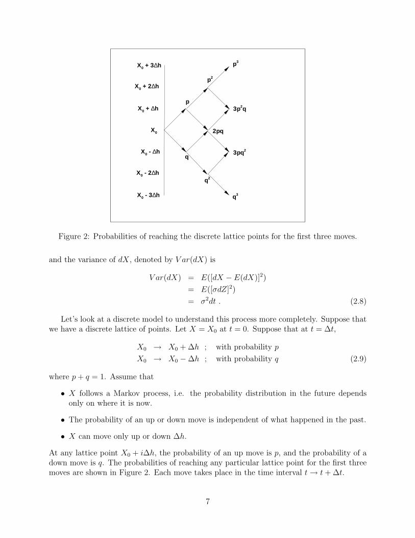
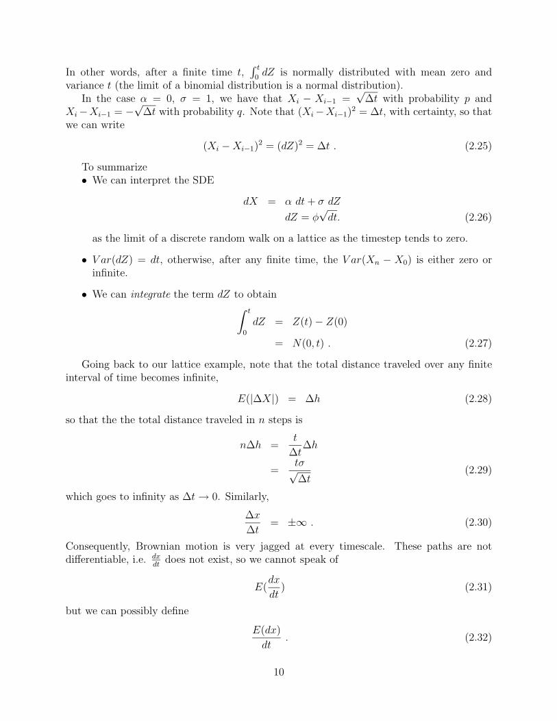
Figure 2: Probabilities of reaching the discrete lattice points for the first three moves.
and the variance of dX, denoted by V ar(dX) is
V ar(dX) = E([dX − E(dX)]2)
= E([σdZ]2)
= σ2dt . (2.8)
Let’s look at a discrete model to understand this process more completely. Suppose thatwe have a discrete lattice of points. Let X = X0 at t = 0. Suppose that at t = ∆t,
X0 → X0 + ∆h ; with probability p
X0 → X0 −∆h ; with probability q (2.9)
where p+ q = 1. Assume that
• X follows a Markov process, i.e. the probability distribution in the future dependsonly on where it is now.
• The probability of an up or down move is independent of what happened in the past.
• X can move only up or down ∆h.
At any lattice point X0 + i∆h, the probability of an up move is p, and the probability of adown move is q. The probabilities of reaching any particular lattice point for the first threemoves are shown in Figure 2. Each move takes place in the time interval t→ t+ ∆t.
7
Let ∆X be the change in X over the interval t→ t+ ∆t. Then
E(∆X) = (p− q)∆hE([∆X]2) = p(∆h)2 + q(−∆h)2
= (∆h)2, (2.10)
so that the variance of ∆X is
V ar(∆X) = E([∆X]2)− [E(∆X)]2
= (∆h)2 − (p− q)2(∆h)2
= 4pq(∆h)2 . (2.11)
Now, suppose we consider the distribution of X after n moves, so that t = n∆t. Theprobability of j up moves, and (n− j) down moves (P (n, j)) is
P (n, j) =n!
j!(n− j)!pjqn−j (2.12)
which is just a binomial distribution. Now, if Xn is the value of X after n steps on thelattice, then
E(Xn −X0) = nE(∆X)
V ar(Xn −X0) = nV ar(∆X) , (2.13)
which follows from the properties of a binomial distribution, (each up or down move isindependent of previous moves). Consequently, from equations (2.10, 2.11, 2.13) we obtain
E(Xn −X0) = n(p− q)∆h
=t
∆t(p− q)∆h
V ar(Xn −X0) = n4pq(∆h)2
=t
∆t4pq(∆h)2 (2.14)
Now, we would like to take the limit at ∆t→ 0 in such a way that the mean and varianceof X, after a finite time t is independent of ∆t, and we would like to recover
dX = αdt + σdZ
E(dX) = αdt
V ar(dX) = σ2dt (2.15)
as ∆t→ 0. Now, since 0 ≤ p, q ≤ 1, we need to choose ∆h = Const√
∆t. Otherwise, fromequation (2.14) we get that V ar(Xn −X0) is either 0 or infinite after a finite time. (Stockvariances do not have either of these properties, so this is obviously not a very interestingcase).
8
Let’s choose ∆h = σ√
∆t, which gives (from equation (2.14))
E(Xn −X0) = (p− q) σt√∆t
V ar(Xn −X0) = t4pqσ2 (2.16)
Now, for E(Xn −X0) to be independent of ∆t as ∆t→ 0, we must have
(p− q) = Const.√
∆t (2.17)
If we choose
p− q =α
σ
√∆t (2.18)
we get
p =1
2[1 +
α
σ
√∆t]
q =1
2[1− α
σ
√∆t] (2.19)
Now, putting together equations (2.16-2.19) gives
E(Xn −X0) = αt
V ar(Xn −X0) = tσ2(1− α2
σ2∆t)
= tσ2 ; ∆t→ 0 (2.20)
so that, in the limit as ∆t→ 0, we can interpret the random walk for X on the lattice (withthese parameters) as the solution to the stochastic differential equation (SDE)
dX = α dt+ σ dZ
dZ = φ√dt. (2.21)
For future reference, if α = 0, σ = 1, so that dX = Xi − Xi−1 = dZ, note that (fromequation (2.19))
E(Xn −X0) = 0
V ar(Xn −X0) = t (2.22)
so that we can write ∫ t
0
dX =
∫ t
0
dZ
= (Xn −X0) (2.23)
where
(Xn −X0) = N(0, t)
=
∫ t
0
dZ . (2.24)
9
In other words, after a finite time t,∫ t
0dZ is normally distributed with mean zero and
variance t (the limit of a binomial distribution is a normal distribution).In the case α = 0, σ = 1, we have that Xi − Xi−1 =
√∆t with probability p and
Xi−Xi−1 = −√
∆t with probability q. Note that (Xi−Xi−1)2 = ∆t, with certainty, so thatwe can write
(Xi −Xi−1)2 = (dZ)2 = ∆t . (2.25)
To summarize• We can interpret the SDE
dX = α dt+ σ dZ
dZ = φ√dt. (2.26)
as the limit of a discrete random walk on a lattice as the timestep tends to zero.
• V ar(dZ) = dt, otherwise, after any finite time, the V ar(Xn − X0) is either zero orinfinite.
• We can integrate the term dZ to obtain∫ t
0
dZ = Z(t)− Z(0)
= N(0, t) . (2.27)
Going back to our lattice example, note that the total distance traveled over any finiteinterval of time becomes infinite,
E(|∆X|) = ∆h (2.28)
so that the the total distance traveled in n steps is
n∆h =t
∆t∆h
=tσ√∆t
(2.29)
which goes to infinity as ∆t→ 0. Similarly,
∆x
∆t= ±∞ . (2.30)
Consequently, Brownian motion is very jagged at every timescale. These paths are notdifferentiable, i.e. dx
dtdoes not exist, so we cannot speak of
E(dx
dt) (2.31)
but we can possibly define
E(dx)
dt. (2.32)
10
0 2 4 6 8 10 12Time (years)
0
100
200
300
400
500
600
700
800
900
1000A
sset
Pric
e ($
)
Risk FreeReturn
Low Volatility Caseσ = .20 per year
0 2 4 6 8 10 12Time (years)
0
100
200
300
400
500
600
700
800
900
1000
Ass
et P
rice
($)
Risk FreeReturn
High Volatility Caseσ = .40 per year
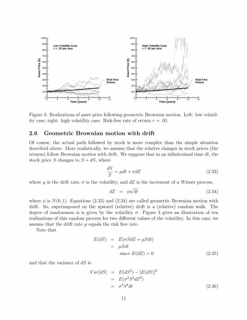
Figure 3: Realizations of asset price following geometric Brownian motion. Left: low volatil-ity case; right: high volatility case. Risk-free rate of return r = .05.
2.6 Geometric Brownian motion with drift
Of course, the actual path followed by stock is more complex than the simple situationdescribed above. More realistically, we assume that the relative changes in stock prices (thereturns) follow Brownian motion with drift. We suppose that in an infinitesimal time dt, thestock price S changes to S + dS, where
dS
S= µdt+ σdZ (2.33)
where µ is the drift rate, σ is the volatility, and dZ is the increment of a Wiener process,
dZ = φ√dt (2.34)
where φ is N(0, 1). Equations (2.33) and (2.34) are called geometric Brownian motion withdrift. So, superimposed on the upward (relative) drift is a (relative) random walk. Thedegree of randomness is is given by the volatility σ. Figure 3 gives an illustration of tenrealizations of this random process for two different values of the volatility. In this case, weassume that the drift rate µ equals the risk free rate.
Note that
E(dS) = E(σSdZ + µSdt)
= µSdt
since E(dZ) = 0 (2.35)
and that the variance of dS is
V ar[dS] = E(dS2)− [E(dS)]2
= E(σ2S2dZ2)
= σ2S2dt (2.36)
11
so that σ is a measure of the degree of randomness of the stock price movement.Equation (2.33) is a stochastic differential equation. The normal rules of calculus don’t
apply, since for example
dZ
dt= φ
1√dt
→∞ as dt→ 0 .
The study of these sorts of equations uses results from stochastic calculus. However, forour purposes, we need only one result, which is Ito’s Lemma (see Derivatives: the theoryand practice of financial engineering, by P. Wilmott). Suppose we have some functionG = G(S, t), where S follows the stochastic process equation (2.33), then, in small timeincrement dt, G→ G+ dG, where
dG =
(µS
∂G
∂S+σ2S2
2
∂2G
∂S2 +∂G
∂t
)dt+ σS
∂G
∂SdZ (2.37)
An informal derivation of this result is given in the following section.
2.6.1 Ito’s Lemma
We give an informal derivation of Ito’s lemma (2.37). Suppose we have a variable S whichfollows
dS = a(S, t)dt+ b(S, t)dZ (2.38)
where dZ is the increment of a Weiner process.Now since
dZ2 = φ2dt (2.39)
where φ is a random variable drawn from a normal distribution with mean zero and unitvariance, we have that, if E is the expectation operator, then
E(φ) = 0 E(φ2) = 1 (2.40)
so that the expected value of dZ2 is
E(dZ2) = dt (2.41)
Now, it can be shown thatE((dZ2 − dt)2) = O(dt2) (2.42)
so that, in the limit as dt → 0, we have that φ2dt becomes non-stochastic, so that withprobability one
dZ2 → dt as dt→ 0 (2.43)
Now, suppose we have some function G = G(S, t), then
dG = GSdS +Gtdt+GSSdS2
2+ ... (2.44)
12
Now (from (2.38) )
(dS)2 = (adt+ b dZ)2
= a2dt2 + ab dZdt+ b2dZ2 (2.45)
Since dZ = O(√dt) and dZ2 → dt, equation (2.45) becomes
(dS)2 = b2dZ2 +O((dt)3/2) (2.46)
or(dS)2 → b2dt as dt→ 0 (2.47)
Now, equations(2.38,2.44,2.47) give
dG = GSdS +Gtdt+GSSdS2
2+ ...
= GS(a dt+ b dZ) + dt(Gt +GSSb2
2)
= GSb dZ + (aGS +GSSb2
2+Gt)dt (2.48)
So, we have the result that if
dS = a(S, t)dt+ b(S, t)dZ (2.49)
and if G = G(S, t), then
dG = GSb dZ + (a GS +GSSb2
2+Gt)dt (2.50)
Equation (2.37) can be deduced by setting a = µS and b = σS in equation (2.50).
2.6.2 Some uses of Ito’s Lemma
Suppose we have
dS = µdt+ σdZ . (2.51)
If µ, σ = Const., then this can be integrated exactly to give
S(t) = S(0) + µt+ σ(Z(t)− Z(0)) (2.52)
and from equation (2.27)
Z(t)− Z(0) = N(0, t) (2.53)
Suppose instead we use the more usual geometric Brownian motion
dS = µSdt+ σSdZ (2.54)
13
Let F (S) = logS, and use Ito’s Lemma
dF = FSSσdZ + (FSµS + FSSσ2S2
2+ Ft)dt
= (µ− σ2
2)dt+ σdZ , (2.55)
so that we can integrate this to get
F (t) = F (0) + (µ− σ2
2)t+ σ(Z(t)− Z(0)) (2.56)
or, since S = eF ,
S(t) = S(0) exp[(µ− σ2
2)t+ σ(Z(t)− Z(0))] . (2.57)
Unfortunately, these cases are about the only situations where we can exactly integrate theSDE (constant σ, µ).
2.7 The Black-Scholes Analysis
Assume• The stock price follows geometric Brownian motion, equation (2.33).
• The risk-free rate of return is a constant r.
• There are no arbitrage opportunities, i.e. all risk-free portfolios must earn the risk-freerate of return.
• Short selling is permitted (i.e. we can own negative quantities of an asset).Suppose that we have an option whose value is given by V = V (S, t). Construct an
imaginary portfolio, consisting of one option, and a number of (−(αh)) of the underlyingasset. (If (αh) > 0, then we have sold the asset short, i.e. we have borrowed an asset, soldit, and are obligated to give it back at some future date).
The value of this portfolio P is
P = V − (αh)S (2.58)
In a small time dt, P → P + dP ,
dP = dV − (αh)dS (2.59)
Note that in equation (2.59) we not included a term (αh)SS. This is actually a rather subtlepoint, since we shall see (later on) that (αh) actually depends on S. However, if we think ofa real situation, at any instant in time, we must choose (αh), and then we hold the portfoliowhile the asset moves randomly. So, equation (2.59) is actually the change in the value of
14
the portfolio, not a differential. If we were taking a true differential then equation (2.59)would be
dP = dV − (αh)dS − Sd(αh)
but we have to remember that (αh) does not change over a small time interval, since we pick(αh), and then S changes randomly. We are not allowed to peek into the future, (otherwise,we could get rich without risk, which is not permitted by the no-arbitrage condition) andhence (αh) is not allowed to contain any information about future asset price movements.The principle of no peeking into the future is why Ito stochastic calculus is used. Other formsof stochastic calculus are used in Physics applications (i.e. turbulent flow).
Substituting equations (2.33) and (2.37) into equation (2.59) gives
dP = σS(VS − (αh)
)dZ +
(µSVS +
σ2S2
2VSS + Vt − µ(αh)S
)dt (2.60)
We can make this portfolio riskless over the time interval dt, by choosing (αh) = VS inequation (2.60). This eliminates the dZ term in equation (2.60). (This is the analogue ofour choice of the amount of stock in the riskless portfolio for the two state tree model.) So,letting
(αh) = VS (2.61)
then substituting equation (2.61) into equation (2.60) gives
dP =
(Vt +
σ2S2
2VSS
)dt (2.62)
Since P is now risk-free in the interval t→ t+ dt, then no-arbitrage says that
dP = rPdt (2.63)
Therefore, equations (2.62) and (2.63) give
rPdt =
(Vt +
σ2S2
2VSS
)dt (2.64)
SinceP = V − (αh)S = V − VSS (2.65)
then substituting equation (2.65) into equation (2.64) gives
Vt +σ2S2
2VSS + rSVS − rV = 0 (2.66)
which is the Black-Scholes equation. Note the rather remarkable fact that equation (2.66) isindependent of the drift rate µ.
Equation (2.66) is solved backwards in time from the option expiry time t = T to thepresent t = 0.
15
2.8 Hedging in Continuous Time
We can construct a hedging strategy based on the solution to the above equation. Supposewe sell an option at price V at t = 0. Then we carry out the following
• We sell one option worth V . (This gives us V in cash initially).
• We borrow (S ∂V∂S− V ) from the bank.
• We buy ∂V∂S
shares at price S.
At every instant in time, we adjust the amount of stock we own so that we always have∂V∂S
shares. Note that this is a dynamic hedge, since we have to continually rebalance theportfolio. Cash will flow into and out of the bank account, in response to changes in S. Ifthe amount in the bank is positive, we receive the risk free rate of return. If negative, thenwe borrow at the risk free rate.
So, our hedging portfolio will be
• Short one option worth V .
• Long ∂V∂S
shares at price S.
• V − S ∂V∂S
cash in the bank account.
At any instant in time (including the terminal time), this portfolio can be liquidated andany obligations implied by the short position in the option can be covered, at zero gain orloss, regardless of the value of S. Note that given the receipt of the cash for the option, thisstrategy is self-financing.
2.9 The option price
So, we can see that the price of the option valued by the Black-Scholes equation is the marketprice of the option at any time. If the price was higher then the Black-Scholes price, we couldconstruct the hedging portfolio, dynamically adjust the hedge, and end up with a positiveamount at the end. Similarly, if the price was lower than the Black-Scholes price, we couldshort the hedging portfolio, and end up with a positive gain. By the no-arbitrage condition,this should not be possible.
Note that we are not trying to predict the price movements of the underlying asset,which is a random process. The value of the option is based on a hedging strategy whichis dynamic, and must be continuously rebalanced. The price is the cost of setting up thehedging portfolio. The Black-Scholes price is not the expected payoff.
The price given by the Black-Scholes price is not the value of the option to a speculator,who buys and holds the option. A speculator is making bets about the underlying drift rateof the stock (note that the drift rate does not appear in the Black-Scholes equation). Fora speculator, the value of the option is given by an equation similar to the Black-Scholesequation, except that the drift rate appears. In this case, the price can be interpreted as theexpected payoff based on the guess for the drift rate. But this is art, not science!
16
2.10 American early exercise
Actually, most options traded are American options, which have the feature that they canbe exercised at any time. Consequently, an investor acting optimally, will always exercisethe option if the value falls below the payoff or exercise value. So, the value of an Americanoption is given by the solution to equation (2.66) with the additional constraint
V (S, t) ≥{
max(S −K, 0) for a callmax(K − S, 0) for a put
(2.67)
Note that since we are working backwards in time, we know what the option is worth infuture, and therefore we can determine the optimal course of action.
In order to write equation (2.66) in more conventional form, define τ = T − t, so thatequation (2.66) becomes
Vτ =σ2S2
2VSS + rSVS − rV
V (S, τ = 0) =
{max(S −K, 0) for a callmax(K − S, 0) for a put
V (0, τ) → Vτ = −rV
V (S =∞, τ) →{' S for a call' 0 for a put
(2.68)
If the option is American, then we also have the additional constraints
V (S, τ) ≥{
max(S −K, 0) for a callmax(K − S, 0) for a put
(2.69)
Define the operator
LV ≡ Vτ − (σ2S2
2VSS + rSVS − rV ) (2.70)
and let V (S, 0) = V ∗. More formally, the American option pricing problem can be stated as
LV ≥ 0
V − V ∗ ≥ 0
(V − V ∗)LV = 0 (2.71)
3 The Risk Neutral World
Suppose instead of valuing an option using the above no-arbitrage argument, we wanted toknow the expected value of the option. We can imagine that we are buying and holding theoption, and not hedging. If we are considering the value of risky cash flows in the future,then these cash flows should be discounted at an appropriate discount rate, which we willcall ρ (i.e. the riskier the cash flows, the higher ρ).
Consequently the value of an option today can be considered to the be the discountedfuture value. This is simply the old idea of net present value. Regard S today as known,
17
and let V (S + dS, t + dt) be the value of the option at some future time t + dt, which isuncertain, since S evolves randomly. Thus
V (S, t) =1
1 + ρdtE(V (S + dS, t+ dt)) (3.1)
where E(...) is the expectation operator, i.e. the expected value of V (S + dS, t + dt) giventhat V = V (S, t) at t = t. We can rewrite equation (3.1) as (ignoring terms of o(dt), whereo(dt) represents terms that go to zero faster than dt )
ρdtV (S, t) = E(V (S, t) + dV )− V (S, t) . (3.2)
Since we regard V as known today, then
E(V (S, t) + dV )− V (S, t) = E(dV ) , (3.3)
so that equation (3.2) becomes
ρdtV (S, t) = E(dV ) . (3.4)
Assume thatdS
S= µdt+ σdZ . (3.5)
From Ito’s Lemma (2.37) we have that
dV =
(Vt +
σ2S2
2VSS + µSVS
)dt+ σSdZ . (3.6)
Noting that
E(dZ) = 0 (3.7)
then
E(dV ) =
(Vt +
σ2S2
2VSS + µSVS
)dt . (3.8)
Combining equations (3.4-3.8) gives
Vt +σ2S2
2VSS + µSVS − ρV = 0 . (3.9)
Equation (3.9) is the PDE for the expected value of an option. If we are not hedging,maybe this is the value that we are interested in, not the no-arbitrage value. However, ifthis is the case, we have to estimate the drift rate µ, and the discount rate ρ. Estimatingthe appropriate discount rate is always a thorny issue.
Now, note the interesting fact, if we set ρ = r and µ = r in equation (3.9) then we simplyget the Black-Scholes equation (2.66).
18
This means that the no-arbitrage price of an option is identical to the expected value ifρ = r and µ = r. In other words, we can determine the no-arbitrage price by pretending weare living in a world where all assets drift at rate r, and all investments are discounted atrate r. This is the so-called risk neutral world.
This result is the source of endless confusion. It is best to think of this as simply amathematical fluke. This does not have any reality. Investors would be very stupid to thinkthat the drift rate of risky investments is r. I’d rather just buy risk-free bonds in this case.There is in reality no such thing as a risk-neutral world. Nevertheless, this result is usefulfor determining the no-arbitrage value of an option using a Monte Carlo approach. Usingthis numerical method, we simply assume that
dS = rSdt+ σSdZ (3.10)
and simulate a large number of random paths. If we know the option payoff as a function ofS at t = T , then we compute
V (S, 0) = e−rTEQ(V (S, T )) (3.11)
which should be the no-arbitrage value.Note the EQ in the above equation. This makes it clear that we are taking the expectation
in the risk neutral world (the expectation in the Q measure). This contrasts with the real-world expectation (the P measure).
4 Monte Carlo Methods
This brings us to the simplest numerical method for computing the no-arbitrage value of anoption. Suppose that we assume that the underlying process is
dS
S= µdt+ σdZ (4.1)
then we can simulate a path forward in time, starting at some price today S0, using a forwardEuler timestepping method
Si+1 = Si + Si(r∆t+ φi√
∆t) (4.2)
where ∆t is the finite timestep, and φi is a random number which is N(0, 1). Note that ateach timestep, we generate a new random number. After N steps, with T = N∆t, we havea single realized path. Given the payoff function of the option, the value for this path wouldbe
V alue = Payoff(SN) . (4.3)
For example, if the option was a European call, then
V alue = max(SN −K, 0)
K = Strike Price (4.4)
19
Suppose we run a series of trials, m = 1, ...,M , and denote the payoff after the m′th trialas payoff(m). Then, the no-arbitrage value of the option is
Option V alue = e−rTE(payoff)
' e−rT1
M
m=M∑m=1
payoff(m) . (4.5)
Recall that these paths are not the real paths, but are the risk neutral paths.Now, we should remember that we are
1. approximating the solution to the SDE by forward Euler, which has O(∆t) truncationerror.
2. approximating the expectation by the mean of many random paths. This Monte Carloerror is of size O(1/
√M), which is slowly converging.
There are thus two sources of error in the Monte Carlo approach: timestepping error andsampling error.
The slow rate of convergence of Monte Carlo methods makes these techniques unattractiveexcept when the option is written on several (i.e. more than three) underlying assets. Aswell, since we are simulating forward in time, we cannot know at a given point in the forwardpath if it is optimal to exercise or hold an American style option. This is easy if we use a PDEmethod, since we solve the PDE backwards in time, so we always know the continuation valueand hence can act optimally. However, if we have more than three factors, PDE methodsbecome very expensive computationally. As well, if we want to determine the effects ofdiscrete hedging, for example, a Monte Carlo approach is very easy to implement.
The error in the Monte Carlo method is then
Error = O
(max(∆t,
1√M
)
)∆t = timestep
M = number of Monte Carlo paths (4.6)
Now, it doesn’t make sense to drive the Monte Carlo error down to zero if there is O(∆t)timestepping error. We should seek to balance the timestepping error and the samplingerror. In order to make these two errors the same order, we should choose M = O( 1
(∆t)2 ).
This makes the total error O(∆t). We also have that
Complexity = O
(M
∆t
)= O
(1
(∆t)3
)∆t = O
((Complexity)−1/3
)(4.7)
and hence
Error = O
(1
( Complexity)1/3
). (4.8)
20
In practice, the convergence in terms of timestep error is often not done. People just picka timestep, i.e. one day, and increase the number of Monte Carlo samples until they achieveconvergence in terms of sampling error, and ignore the timestep error. Sometimes this givesbad results!
Note that the exact solution to Geometric Brownian motion (2.57) has the property thatthe asset value S can never reach S = 0 if S(0) > 0, in any finite time. However, due to theapproximate nature of our Forward Euler method for solving the SDE, it is possible that anegative or zero Si can show up. We can do one of three things here, in this case
• Cut back the timestep at this point in the simulation so that S is positive.
• Set S = 0 and continue. In this case, S remains zero for the rest of this particularsimulation.
• Use Ito’s Lemma, and determine the SDE for logS, i.e. if F = logS, then, fromequation (2.55), we obtain (with µ = r)
dF = (r − σ2
2)dt+ σdZ , (4.9)
so that now, if F < 0, there is no problem, since S = eF , and if F < 0, this just meansthat S is very small. We can use this idea for any stochastic process where the variableshould not go negative.
Usually, most people set S = 0 and continue. As long as the timestep is not too large,this situation is probably due to an event of low probability, hence any errors incurred willnot affect the expected value very much. If negative S values show up many times, this is asignal that the timestep is too large.
In the case of simple Geometric Brownian motion, where r, σ are constants, then the SDEcan be solved exactly, and we can avoid timestepping errors (see Section 2.6.2). In this case
S(T ) = S(0) exp[(r − σ2
2)T + σφ
√T ] (4.10)
where φ = N(0, 1). I’ll remind you that equation (4.10) is exact. For these simple cases,we should always use equation (4.10). Unfortunately, this does not work in more realisticsituations.
Monte Carlo is popular because
• It is simple to code. Easily handles complex path dependence.
• Easily handles multiple assets.
The disadvantages of Monte Carlo methods are
• It is difficult to apply this idea to problems involving optimal decision making (e.g.American options).
• It is hard to compute the Greeks (VS, VSS), which are the hedging parameters, veryaccurately.
• MC converges slowly.
21
4.1 Monte Carlo Error Estimators
The sampling error can be estimated via a statistical approach. If the estimated mean ofthe sample is
µ =e−rT
M
m=M∑m=1
payoff(m) (4.11)
and the standard deviation of the estimate is
ω =
(1
M − 1
m=M∑m=1
(e−rTpayoff(m)− µ)2
)1/2
(4.12)
then the 95% confidence interval for the actual value V of the option is
µ− 1.96ω√M
< V < µ+1.96ω√M
(4.13)
Note that in order to reduce this error by a factor of 10, the number of simulations must beincreased by 100.
The timestep error can be estimated by running the problem with different size timesteps,comparing the solutions.
4.2 Random Numbers and Monte Carlo
There are many good algorithms for generating random sequences which are uniformly dis-tributed in [0, 1]. See for example, (Numerical Recipies in C++., Press et al, CambridgeUniversity Press, 2002). As pointed out in this book, often the system supplied randomnumber generators, such as rand in the standard C library, and the infamous RANDU IBMfunction, are extremely bad. The Matlab functions appear to be quite good. For moredetails, please look at (Park and Miller, ACM Transactions on Mathematical Software, 31(1988) 1192-1201).
However, we need random numbers which are normally distributed on [−∞,+∞], withmean zero and variance one (N(0, 1)).
Suppose we have uniformly distributed numbers on [0, 1], i.e. the probability of obtaininga number between x and x+ dx is
p(x)dx = dx ; 0 ≤ x ≤ 1
= 0 ; otherwise (4.14)
Let’s take a function of this random variable y(x). How is y(x) distributed? Let p(y) be theprobability distribution of obtaining y in [y, y + dy]. Consequently, we must have
p(x)|dx| = p(y)|dy|
or
p(y) = p(x)|dxdy| . (4.15)
22
Suppose we want p(y) to be normal,
p(y) =e−y
2/2
√2π
. (4.16)
If we start with a uniform distribution, p(x) = 1 on [0, 1], then from equations (4.15-4.16)we obtain
dx
dy=
e−y2/2
√2π
. (4.17)
Now, for x ∈ [0, 1], we have that the probability of obtaining a number in [0, x] is∫ x
0
dx′ = x , (4.18)
but from equation (4.17) we have
dx′ =e−(y′)2/2
√2π
dy′ . (4.19)
So, there exists a y such that the probability of getting a y′ in [−∞, y] is equal to theprobability of getting x′ in [0, x],∫ x
0
dx′ =
∫ y
−∞
e−(y′)2/2
√2π
dy′ , (4.20)
or
x =
∫ y
−∞
e−(y′)2/2
√2π
dy′ . (4.21)
So, if we generate uniformly distributed numbers x on [0, 1], then to determine y which areN(0, 1), we do the following
• Generate x
• Find y such that
x =1√2π
∫ y
−∞e−(y′)2/2dy′ . (4.22)
We can write this last step as
y = F (x) (4.23)
where F (x) is the inverse cumulative normal distribution.
23
4.3 The Box-Muller Algorithm
Starting from random numbers which are uniformly distributed on [0, 1], there is actually asimpler method for obtaining random numbers which are normally distributed.
If p(x) is the probability of finding x ∈ [x, x + dx] and if y = y(x), and p(y) is theprobability of finding y ∈ [y, y + dy], then, from equation (4.15) we have
|p(x)dx| = |p(y)dy| (4.24)
or
p(y) = p(x)
∣∣∣∣dxdy∣∣∣∣ . (4.25)
Now, suppose we have two original random variables x1, x2, and let p(xi, x2) be theprobability of obtaining (x1, x2) in [x1, x1 + dx1]× [x2, x2 + dx2]. Then, if
y1 = y1(x1, x2)
y2 = y2(x1, x2) (4.26)
and we have that
p(y1, y2) = p(x1, x2)|∂(x1, x2)
∂(y1, y2)(4.27)
where the Jacobian of the transformation is defined as
∂(x1, x2)
∂(y1, y2)= det
∣∣∣∣∣ ∂x1
∂y1
∂x1
∂y2∂x2
∂y1
∂x2
∂y2
∣∣∣∣∣ (4.28)
Recall that the Jacobian of the transformation can be regarded as the scaling factor whichtransforms dx1 dx2 to dy1 dy2, i.e.
dx1 dx2 =
∣∣∣∣∂(x1, x2)
∂(y1, y2)
∣∣∣∣ dy1 dy2 . (4.29)
Now, suppose that we have x1, x2 uniformly distributed on [0, 1]× [0, 1], i.e.
p(x1, x2) = U(x1)U(x2) (4.30)
where
U(x) = 1 ; 0 ≤ x ≤ 1
= 0 ; otherwise . (4.31)
We denote this distribution as x1 ' U [0, 1] and x2 ' U [0, 1].If p(x1, x2) is given by equation (4.30), then we have from equation (4.27) that
p(y1, y2) = |∂(x1, x2)
∂(y1, y2)| (4.32)
24
Now, we want to find a transformation y1 = y1(x1, x2), y2 = y2(x1, x2) which results in normaldistributions for y1, y2. Consider
y1 =√−2 log x1 cos 2πx2
y2 =√−2 log x1 sin 2πx2 (4.33)
or solving for (x2, x2)
x1 = exp
(−1
2(y2
1 + y22)
)x2 =
1
2πtan−1
[y2
y1
]. (4.34)
After some tedious algebra, we can see that (using equation (4.34))∣∣∣∣∂(x1, x2)
∂(y1, y2)
∣∣∣∣ =1√2πe−y
21/2
1√2πe−y
22/2 (4.35)
Now, assuming that equation (4.30) holds, then from equations (4.32-4.35) we have
p(y1, y2) =1√2πe−y
21/2
1√2πe−y
22/2 (4.36)
so that (y1, y2) are independent, normally distributed random variables, with mean zero andvariance one, or
y1 ' N(0, 1) ; y2 ' N(0, 1) . (4.37)
Box Muller Algorithm
RepeatGenerate u1 ' U(0, 1), u2 ' U(0, 1)θ = 2πu2, ρ =
√−2 log u1
z1 = ρ cos θ; z2 = ρ sin θEnd Repeat
(4.38)
This has the effect that Z1 ' N(0, 1) and Z2 ' N(0, 1).Note that we generate two draws from a normal distribution on each pass through the
loop.
4.3.1 An improved Box Muller
The algorithm (4.38) can be expensive due to the trigonometric function evaluations. Wecan use the following method to avoid these evaluations. Let
U1 ' U [0, 1] ; U2 ' U [0, 1]
V1 = 2U1 − 1 ; V2 = 2U2 − 1 (4.39)
which means that (V1, V2) are uniformly distributed in [0, 1]× [0, 1]. Now, we carry out thefollowing procedure
25
Rejection Method
RepeatIf ( V 2
1 + V 22 < 1 )
AcceptElse
RejectEndif
End Repeat
(4.40)
which means that if we define (V1, V2) as in equation (4.39), and then process the pairs(V1, V2) using algorithm (4.40) we have that (V1, V2) are uniformly distributed on the diskcentered at the origin, with radiius one, in the (V1, V2) plane. This is denoted by
(V1, V2) ' D(0, 1) . (4.41)
If (V1, V2) ' D(0, 1) and R2 = V 21 + V 2
2 , then the probability of finding R in [R,R+ dR]is
p(R) dR =2πR dR
π(1)2
= 2R dR . (4.42)
From the fundamental law of transformation of probabilities, we have that
p(R2)d(R2) = p(R)dR
= 2R dR (4.43)
so that
p(R2) =2Rd(R2)dR
= 1 (4.44)
so that R2 is uniformly distributed on [0, 1], (R ' U [0, 1]).As well, if θ = tan−1(V2/V1), i.e. θ is the angle between a line from the origin to the
point (V1, V2) and the V1 axis, then θ ' U [0, 2π]. Note that
cos θ =V1√
V 21 + V 2
2
sin θ =V2√
V 21 + V 2
2
. (4.45)
Now in the original Box Muller algorithm (4.38),
θ = U1 ' U [0, 2π]
U2 ' U [0, 1] , (4.46)
26
but θ = tan−1(V2/V1) ' U [0, 2π], and R2 = U [0, 1]. Therefore, if we let W = R2, then wecan replace θ, ρ in algorithm (4.38) by
θ = tan−1
(V2
V1
)ρ =
√−2 logW . (4.47)
Now, the last step in the Box Muller algorithm (4.38) is
Z1 = ρ cos θ
Z2 = ρ sin θ , (4.48)
but if (V1, V2) ' D(0, 1), then
Z1 = ρV1√W
Z2 = ρV2√W
. (4.49)
This leads to the following algorithm
Polar form of Box Muller
RepeatGenerate U1 ' U [0, 1], U2 ' U [0, 1].Let
V1 = 2U1 − 1
V2 = 2U2 − 1
W = V 21 + V 2
2
If( W < 1) then
Z1 = V1
√−2 logW/W
Z2 = V2
√−2 logW/W (4.50)
End IfEnd Repeat
Consequently, (Z1, Z2) are independent (uncorrelated), and Z1 ' N(0, 1), and Z2 ' N(0, 1).Because of the rejection step (4.40), about (1 − π/4) of the random draws in [−1,+1] ×[−1,+1] are rejected (about 21%), but this method is still generally more efficient that bruteforce Box Muller.
27
4.4 Speeding up Monte Carlo
Monte Carlo methods are slow to converge, since the error is given by
Error = O(1√M
)
where M is the number of samples. There are many methods which can be used to try tospeed up convergence. These are usually termed Variance Reduction techniques.
Perhaps the simplest idea is the Antithetic Variable method. Suppose we compute arandom asset path
Si+1 = Siµ∆t+ Siσφi√
∆t
where φi are N(0, 1). We store all the φi, i = 1, ..., for a given path. Call the estimate forthe option price from this sample path V +. Then compute a second sample path where(φi)′ = −φi, i = 1, ...,. Call this estimate V −. Then compute the average
V =V + + V −
2,
and continue sampling in this way. Averaging over all the V , slightly faster convergence isobtained. Intuitively, we can see that this symmetrizes the random paths.
Let X+ be the option values obtained from all the V + simulations, and X− be theestimates obtained from all the V − simulations. Note that V ar(X+) = V ar(X−) (they havethe same distribution). Then
V ar(X+ +X−
2) =
1
4V ar(X+) +
1
4V ar(X−) +
1
2Cov(X+, X−)
=1
2V ar(X+) +
1
2Cov(X+, X−) (4.51)
which will be smaller than V ar(X+) if Cov(X+, X−) is nonpositive.Note that this method can be used to estimate the mean. In the MC error estimator
(4.13), compute the standard deviation of the estimator as ω =√V ar(X
++X−
2).
However, if we want to estimate the distribution of option prices (i.e. a probabilitydistribution), then we should not average each V + and V −, since this changes the varianceof the actual distribution.
If we want to know the actual variance of the distribution (and not just the mean),then to compute the variance of the distribution, we should just use the estimates V +, andcompute the estimate of the variance in the usual way. This should also be used if we wantto plot a histogram of the distribution, or compute the Value at Risk.
28
4.5 Estimating the mean and variance
An estimate of the mean x and variance s2M of M numbers x1, x2, ..., xM is
s2M =
1
M − 1
M∑i=1
(xi − x)2
x =1
M
M∑i=1
xi (4.52)
Alternatively, one can use
s2M =
1
M − 1
M∑i=1
x2i −
1
M
(M∑i=1
xi
)2 (4.53)
which has the advantage that the estimate of the mean and standard deviation can becomputed in one loop.
In order to avoid roundoff, the following method is suggested by Seydel (R. Seydel, Toolsfor Computational Finance, Springer, 2002). Set
α1 = x1 ; β1 = 0 (4.54)
then compute recursively
αi = αi−1 +xi − αi−1
i
βi = βi−1 +(i− 1)(xi − αi−1)2
i(4.55)
so that
x = αM
s2M =
βMM − 1
(4.56)
4.6 Low Discrepancy Sequences
In a effort to get around the 1√M
, (M = number of samples) behaviour of Monte Carlomethods, quasi-Monte Carlo methods have been devised.
These techniques use a deterministic sequence of numbers (low discrepancy sequences).The idea here is that a Monte Carlo method does not fill the sample space very evenly (afterall, its random). A low discrepancy sequence tends to sample the space in a orderly fashion.If d is the dimension of the space, then the worst case error bound for an LDS method is
Error = O
((logM)d
M
)(4.57)
29
where M is the number of samples used. Clearly, if d is small, then this error bound is (atleast asymptotically) better than Monte Carlo.
LDS methods generate numbers on [0, 1]. We cannot use the Box-Muller method in thiscase to produce normally distributed numbers, since these numbers are deterministic. Wehave to invert the cumulative normal distribution in order to get the numbers distributed withmean zero and standard deviation one on [−∞,+∞]. So, if F (x) is the inverse cumulativenormal distribution, then
xLDS = uniformly distributed on [0, 1]
yLDS = F (xLDS) is N(0, 1) . (4.58)
Another problem has to do with the fact that if we are stepping through time, i.e.
Sn+1 = Sn + Sn(r∆t+ φσ√
∆t)
φ = N(0, 1) (4.59)
with, say, N steps in total, then we need to think of this as a problem in N dimensionalspace. In other words, the k − th timestep is sampled from the k − th coordinate in this Ndimensional space. We are trying to uniformly sample from this N dimensional space.
Let x be a vector of LDS numbers on [0, 1], in N dimensional space
x =
x1
x2
|xN
. (4.60)
So, an LDS algorithm would proceed as follows, for the j′th trial
• Generate xj (the j′th LDS number in an N dimensional space).
• Generate the normally distributed vector yj by inverting the cumulative normal dis-tribution for each component
yj =
F (xj1)
F (xj2)|
F (xjN)
(4.61)
• Generate a complete sample path k = 0, ..., N − 1
Sk+1j = Skj + Skj (r∆t+ yjk+1σ
√∆t)
(4.62)
• Compute the payoff at S = SNj
The option value is the average of these trials.There are a variety of LDS numbers: Halton, Sobol, Niederrieter, etc. Our tests seem to
indicate that Sobol is the best.
30
Note that the worst case error bound for the error is given by equation (4.57). If we usea reasonable number of timesteps, say 50− 100, then, d = 50− 100, which gives a very baderror bound. For d large, the numerator in equation (4.57) dominates. The denominatoronly dominates when
M ' ed (4.63)
which is a very large number of trials for d ' 100. Fortunately, at least for path-dependentoptions, we have found that things are not quite this bad, and LDS seems to work if thenumber of timesteps is less than 100− 200. However, once the dimensionality gets above afew hundred, convergence seems to slow down.
4.7 Correlated Random Numbers
In many cases involving multiple assets, we would like to generate correlated, normallydistributed random numbers. Suppose we have i = 1, ..., d assets, and each asset follows thesimulated path
Sn+1i = Sni + Sni (r∆t+ φni σ
√∆t)
(4.64)
where φni is N(0, 1) and
E(φni φnj ) = ρij (4.65)
where ρij is the correlation between asset i and asset j.Now, it is easy to generate a set of d uncorrelated N(0, 1) variables. Call these ε1, ..., εd.
So, how do we produce correlated numbers? Let
[Ψ]ij = ρij (4.66)
be the matrix of correlation coefficients. Assume that this matrix is SPD (if not, one ofthe random variables is a linear combination of the others, hence this is a degenerate case).Assuming Ψ is SPD, we can Cholesky factor Ψ = LLt, so that
ρij =∑k
LikLtkj (4.67)
Let φ be the vector of correlated normally distributed random numbers (i.e. what we wantto get), and let ε be the vector of uncorrelated N(0, 1) numbers (i.e. what we are given).
φ =
φ1
φ2
|φd
; ε =
ε1ε2|εd
(4.68)
31
So, given ε, we have
E(εiεj) = δij
where
δij = 0 ; if i 6= j
= 1 ; if i = j .
since the εi are uncorrelated. Now, let
φi =∑j
Lijεj (4.69)
which gives
φiφk =∑j
∑l
LijLklεlεj
=∑j
∑l
LijεlεjLtlk . (4.70)
Now,
E(φiφk) = E
[∑j
∑l
LijεlεjLtlk
]=
∑j
∑l
LijE(εlεj)Ltlk
=∑j
∑l
LijδljLtlk
=∑l
LilLtlk
= ρij (4.71)
So, in order to generate correlated N(0, 1) numbers:
• Factor the correlation matrix Ψ = LLt
• Generate uncorrelated N(0, 1) numbers εi
• Correlated numbers φi are given from
φ = Lε
32
5 The Binomial Model
We have seen that a problem with the Monte Carlo method is that it is difficult to use forvaluing American style options. Recall that the holder of an American option can exercisethe option at any time and receive the payoff. In order to determine whether or not it isworthwhile to hold the option, we have to compare the value of continuing to hold the option(the continuation value) with the payoff. If the continuation value is greater than the payoff,then we hold; otherwise, we exercise.
At any point in time, the continuation value depends on what happens in the future.Clearly, if we simulate forward in time, as in the Monte Carlo approach, we don’t know whathappens in the future, and hence we don’t know how to act optimally. This is actually adynamic programming problem. These sorts of problems are usually solved by proceedingfrom the end point backwards. We use the same idea here. We have to start from theterminal time and work backwards.
Recall that we can determine the no-arbitrage value of an option by pretending we live ina risk-neutral world, where risky assets drift at r and are discounted at r. If we let X = logS,then the risk neutral process for X is (from equation (2.55) )
dX = (r − σ2
2)dt+ σdZ . (5.1)
Now, we can construct a discrete approximation to this random walk using the lattice dis-cussed in in Section 2.5. In fact, all we have to do is let let α = r − σ2
2, so that equation
(5.1) is formally identical to equation (2.4). In order to ensure that in the limit as ∆t→ 0,we get the process (5.1), we require that the sizes of the random jumps are ∆X = σ
√∆t
and that the probabilities of up (p) and down (q) moves are
pr =1
2[1 +
α
σ
√∆t]
=1
2[1 +
( rσ− σ
2
)√∆t]
qr =1
2[1− α
σ
√∆t]
=1
2[1−
( rσ− σ
2
)√∆t] , (5.2)
where we have denoted the risk neutral probabilities by pr and qr to distinguish them fromthe real probabilities p, q.
Now, we will switch to a more common notation. If we are at node j, timestep n, we willdenote this node location by Xn
j . Recall that X = logS, so that in terms of asset price, this
is Snj = eXnj .
Now, consider that at node (j, n), the asset can move up with probability pr and downwith probability qr. In other words
Snj → Sn+1j+1 ; with probability pr
Snj → Sn+1j ; with probability qr
(5.3)
33
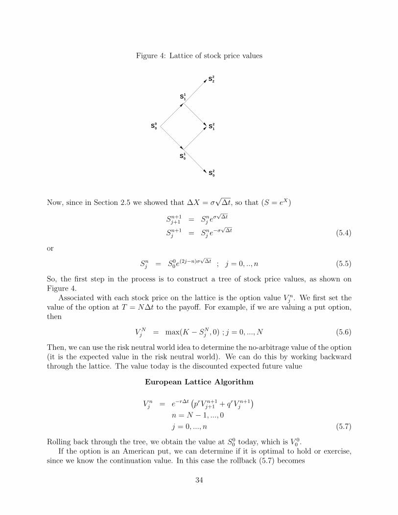
Figure 4: Lattice of stock price values
S00
S11
S01
S22
S12
S02
Now, since in Section 2.5 we showed that ∆X = σ√
∆t, so that (S = eX)
Sn+1j+1 = Snj e
σ√
∆t
Sn+1j = Snj e
−σ√
∆t (5.4)
or
Snj = S00e
(2j−n)σ√
∆t ; j = 0, .., n (5.5)
So, the first step in the process is to construct a tree of stock price values, as shown onFigure 4.
Associated with each stock price on the lattice is the option value V nj . We first set the
value of the option at T = N∆t to the payoff. For example, if we are valuing a put option,then
V Nj = max(K − SNj , 0) ; j = 0, ..., N (5.6)
Then, we can use the risk neutral world idea to determine the no-arbitrage value of the option(it is the expected value in the risk neutral world). We can do this by working backwardthrough the lattice. The value today is the discounted expected future value
European Lattice Algorithm
V nj = e−r∆t
(prV n+1
j+1 + qrV n+1j
)n = N − 1, ..., 0
j = 0, ..., n (5.7)
Rolling back through the tree, we obtain the value at S00 today, which is V 0
0 .If the option is an American put, we can determine if it is optimal to hold or exercise,
since we know the continuation value. In this case the rollback (5.7) becomes
34
American Lattice Algorithm
(V nj )c = e−r∆t
(prV n+1
j+1 + qrV n+1j
)V nj = max
((V n
j )c,max(K − Snj , 0))
n = N − 1, ..., 0
j = 0, ..., n (5.8)
which is illustrated in Figure 5.The binomial lattice method has the following advantages
• It is very easy to code for simple cases.
• It is easy to explain to managers.
• American options are easy to handle.
However, the binomial lattice method has the following disadvantages
• Except for simple cases, coding becomes complex. For example, if we want to handlesimple barrier options, things become nightmarish.
• This method is algebraically identical to an explicit finite difference solution of theBlack-Scholes equation. Consequently, convergence is at an O(∆t) rate.
• The probabilities pr, qr are not real probabilities, they are simply the coefficients ina particular discretization of a PDE. Regarding them as probabilities leads to muchfuzzy thinking, and complex wrong-headed arguments.
If we are going to solve the Black-Scholes PDE, we might as well do it right, and not foolaround with lattices.
5.1 A No-arbitrage Lattice
We can also derive the lattice method directly from the discrete lattice model in Section 2.5.Suppose we assume that
dS = µSdt+ σSdZ (5.9)
and letting X = logS, we have that
dX = (µ− σ2
2)dt+ σdZ (5.10)
so that α = µ − σ2
2in equation (2.19). Now, let’s consider the usual hedging portfolio at
t = n∆t, S = Snj ,
P nj = V n
j − (αh)Snj , (5.11)
35
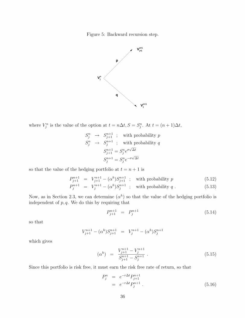
Figure 5: Backward recursion step.
Vjn
Vjn + + 1 1
Vjn+1
p
q
where V nj is the value of the option at t = n∆t, S = Snj . At t = (n+ 1)∆t,
Snj → Sn+1j+1 ; with probability p
Snj → Sn+1j ; with probability q
Sn+1j+1 = Snj e
σ√
∆t
Sn+1j = Snj e
−σ√
∆t
so that the value of the hedging portfolio at t = n+ 1 is
P n+1j+1 = V n+1
j+1 − (αh)Sn+1j+1 ; with probability p (5.12)
P n+1j = V n+1
j − (αh)Sn+1j ; with probability q . (5.13)
Now, as in Section 2.3, we can determine (αh) so that the value of the hedging portfolio isindependent of p, q. We do this by requiring that
P n+1j+1 = P n+1
j (5.14)
so that
V n+1j+1 − (αh)Sn+1
j+1 = V n+1j − (αh)Sn+1
j
which gives
(αh) =V n+1j+1 − V n+1
j
Sn+1j+1 − Sn+1
j
. (5.15)
Since this portfolio is risk free, it must earn the risk free rate of return, so that
P nj = e−r∆tP n+1
j+1
= e−r∆tP n+1j . (5.16)
36
Now, substitute for P nj from equation (5.11), with P n+1
j+1 from equation (5.13), and (αh) fromequation (5.15) gives
V nj = e−r∆t
(pr∗V n+1
j+1 + qr∗V n+1j
)pr∗ =
er∆t − e−σ√
∆t
eσ√
∆t − e−σ√
∆t
qr∗ = 1− pr∗ . (5.17)
Note that pr∗, qr∗ do not depend on the real drift rate µ, which is expected. If we expandpr∗, qr∗ in a Taylor Series, and compare with the pr, qr in equations (5.2), we can show that
pr∗ = pr +O((∆t)3/2)
qr∗ = qr +O((∆t)3/2) . (5.18)
After a bit more work, one can show that the value of the option at t = 0, V 00 using either
pr∗, qr∗ or pr, qr is the same to O(∆t), which is not surprising, since these methods can bothbe regarded as an explicit finite difference approximation to the Black-Scholes equation,having truncation error O(∆t). The definition pr∗, qr∗ is the common definition in financebooks, since the tree has no-arbitrage.
What is the meaning of a no-arbitrage tree? If we are sitting at node Snj , and assumingthat there are only two possible future states
Snj → Sn+1j+1 ; with probability p
Snj → Sn+1j ; with probability q
then using (αh) from equation (5.15) guarantees that the hedging portfolio has the samevalue in both future states.
But let’s be a bit more sensible here. Suppose we are hedging a portfolio of RIM stock.Let ∆t = one day. Suppose the price of RIM stocks is $10 today. Do we actually believethat tomorrow there are only two possible prices for Rim stock
Sup = 10eσ√
∆t
Sdown = 10e−σ√
∆t ?
(5.19)
Of course not. This is obviously a highly simplified model. The fact that there is no-arbitragein the context of the simplified model does not really have a lot of relevance to the real-worldsituation. The best that can be said is that if the Black-Scholes model was perfect, thenwe have that the portfolio hedging ratios computed using either pr, qr or pr∗, qr∗ are bothcorrect to O(∆t).
5.2 More on Ito’s Lemma
In Section 2.6.1, we mysteriously made the infamous comment
37
...it can be shown that dX2 → dt as dt→ 0
In this Section, we will give some justification this remark. For a lot more details here,we refer the reader to Stochastic Differential Equations, by Bernt Oksendal, Springer, 1998.
We have to go back here, and decide what the statement
dX = αdt + σdZ (5.20)
really means. The only sensible interpretation of this is
X(t)−X(0) =
∫ t
0
α(X(s), s)ds+
∫ t
0
σ(X(s), s)dZ(s) . (5.21)
where we can interpret the integrals as the limit, as ∆t→ 0 of a discrete sum. For example,∫ t
0
σ(X(s), s)dZ(s) = lim∆t→0
∑j
σj∆Zj (5.22)
In particular, in order to derive Ito’s Lemma, we have to decide what∫ t
0
c(X, s)dZ2 (5.23)
means. Replace the integral by a sum,∫ t
0
c(X, s)dZ2 '∑j
c(Xj, tj)∆Z2j (5.24)
where
∆Zj = Zj+1 − Zjtj = j∆t . (5.25)
Note that we have evaluated the integral using the left hand end point of each subinterval(the no peaking into the future principle). Now, we claim that∫ t
0
c(X, s)dZ2(s) =
∫ t
0
c(X, s)dt (5.26)
i.e. we can say that dZ2 → dt as dt→ 0. Let’s examine the expression
E
(∑j
cj∆Z2j −
∑j
cj∆t
)2 (5.27)
If equation (5.27) tends to zero as ∆t→ 0, then we can say that
dZ2 → dt (5.28)
38
with probability one as ∆t→ 0. Now, expanding equation (5.27) gives
E
(∑j
cj∆Z2j −
∑j
cj∆t
)2 =
∑ij
E[cj(∆Z
2j −∆t)ci(∆Z
2i −∆t)
]. (5.29)
Now, we assume that
E[cj(∆Z
2j −∆t)ci(∆Z
2i −∆t)
]= δijE
[c2i (∆Z
2i −∆t)2
](5.30)
which means that cj(∆Z2j −∆t) and ci(∆Z
2i −∆t) are independent if i 6= j. We also assume
that
E[c2j(∆Z
2j −∆t)2] = E[c2
j ] E[(∆Z2j −∆t)2] (5.31)
which means that cj and (∆Z2j −∆t) are also assumed to be independent.
Using equations (5.30-5.31), then equation (5.29) becomes∑ij
E[cj(∆Z
2j −∆t) ci(∆Z
2i −∆t)
]=
∑i
E[c2i ] E
[(∆Z2
i −∆t)2]. (5.32)
Now, ∑i
E[c2i ] E
[(∆Z2
i −∆t)2]
=∑i
E[c2i ](E[∆Z4
i
]− 2∆tE
[∆Z2
i
]+ (∆t)2
). (5.33)
Recall that (∆Z)2 is N(0,∆t) ( normally distributed with mean zero and variance ∆t) sothat
E[(∆Zi)
2]
= ∆t
E[(∆Zi)
4]
= 3(∆t)2 (5.34)
so that equation (5.33) becomes
E[∆Z4
i
]− 2∆tE
[∆Z2
i
]+ (∆t)2 = 2(∆t)2 (5.35)
and ∑i
E[c2i ] E
[(∆Z2
i −∆t)2]
= 2∑i
E[c2i ](∆t)
2
= 2∆t
(∑i
E[c2i ]∆t
)= O(∆t) (5.36)
so that we have
E
(∑cj∆Z
2j −
∑j
cj∆t
)2
= O(∆t) (5.37)
or
E
(∑cj∆Z
2j −
∫ t
0
c(s,X(s))ds
)2
= O(∆t) ; as ∆t→ 0 (5.38)
so that in this sense we can write
dZ2 → dt ; dt→ 0 . (5.39)
39
6 Derivative Contracts on non-traded Assets and Real
Options
The hedging arguments used in previous sections use the underlying asset to construct a hedg-ing portfolio. What if the underlying asset cannot be bought and sold, or is non-storable? Ifthe underlying variable is an interest rate, we can’t store this. Or if the underlying asset isbandwidth, we can’t store this either. However, we can get around this using the followingapproach.
6.1 Derivative Contracts
Let the underlying variable follow
dS = a(S, t)dt+ b(S, t)dZ, (6.1)
and let F = F (S, t), so that from Ito’s Lemma
dF =
[aFS +
b2
2FSS + Ft
]dt+ bFSdZ, (6.2)
or in shorter form
dF = µdt+ σ∗dZ
µ = aFS +b2
2FSS + Ft
σ∗ = bFS . (6.3)
Now, instead of hedging with the underlying asset, we will hedge one contract withanother. Suppose we have two contracts F1, F2 (they could have different maturities forexample). Then
dF1 = µ1dt+ σ∗1dZ
dF2 = µ2dt+ σ∗2dZ
µi = a(Fi)S +b2
2(Fi)SS + (Fi)t
σ∗i = b(Fi)S ; i = 1, 2 . (6.4)
Consider the portfolio P such that (recall that ∆1,∆2 are constant over the hedging interval)
P = ∆1F1 + ∆2F2
dP = ∆1 (µ1dt+ σ∗1dZ) + ∆2 (µ2dt+ σ∗2dZ) (6.5)
We can eliminate the random term by choosing
∆1 = σ∗2∆2 = −σ∗1 (6.6)
40
so that
dP = (σ∗2µ1 − σ∗1µ2)dt (6.7)
Since this portfolio is riskless, it must earn the risk-free rate of return,
(σ∗2µ1 − σ∗1µ2)dt = r(∆1F1 + ∆2F2)dt (6.8)
and after some simplification we obtain
µ1 − rF1
σ∗1=
µ2 − rF2
σ∗2(6.9)
Let λS(S, t) be the value of both sides of equation (6.9), so that
µ1 − rF1
σ∗1= λS(S, t)
µ2 − rF2
σ∗2= λS(S, t) . (6.10)
Dropping the subscripts, we obtain
µ− rF1
σ∗= λS (6.11)
Substituting µ, σ∗ from equations (6.3) into equation (6.11) gives
Ft +b2
2FSS + (a− λSb)FS − rF = 0 . (6.12)
Equation (6.12) is the PDE satisfied by a derivative contract on any asset S, traded or not.Suppose
µ = Fµ′
σ∗ = Fσ′ (6.13)
so that we can write
dF = Fµ′dt+ Fσ′dZ (6.14)
then using equation (6.13) in equation (6.11) gives
µ′ = r + λSσ′ (6.15)
which has the convenient interpretation that the expected return on holding (not hedging)the derivative contract F is the risk-free rate plus extra compensation due to the riskiness ofholding F . The extra return is λSσ
′, where λS is the market price of risk of S (which shouldbe the same for all contracts depending on S) and σ′ is the volatility of F . Note that thevolatility and drift of F are not the volatility and drift of the underlying asset S.
41
If S is a traded asset, it must satisfy equation (6.12). Substituting F = S into equation(6.13) gives (a − λSb) = rS, so that F then satisfies the usual Black-Scholes equation ifb = σS.
If we believe that the Capital Asset Pricing Model holds, then a simple minded idea isto estimate
λS = ρSMλM (6.16)
where λM is the price of risk of the market portfolio, and ρSM is the correlation of returnsbetween S and the returns of the market portfolio.
Another idea is the following. Suppose we can find some companies whose main sourceof business is based on S. Let qi be the price of this companies stock at t = ti. The returnof the stock over ti − ti−1 is
Ri =qi − qi−1
qi−1
.
Let RMi be the return of the market portfolio (i.e. a broad index) over the same period. We
compute β as the best fit linear regression to
Ri = α + βRMi
which means that
β =Cov(R,RM)
V ar(RM). (6.17)
Now, from CAPM we have that
E(R) = r + β[E(RM)− r
](6.18)
where E(...) is the expectation operator. We would like to determine the unlevered β, denotedby βu, which is the β for an investment made using equity only. In other words, if the firm weused to compute the β above has significant debt, its riskiness with respect to S is amplified.The unlevered β can be computed by
βu =E
E + (1− Tc)Dβ (6.19)
where
D = long term debt
E = Total market capitalization
Tc = Corporate Tax rate . (6.20)
So, now the expected return from a pure equity investment based on S is
E(Ru) = r+ βu[E(RM)− r
]. (6.21)
42
If we assume that F in equation (6.14) is the company stock, then
µ′ = E(Ru)
= r + βu[E(RM)− r
](6.22)
But equation (6.15) says that
µ′ = r + λSσ′ . (6.23)
Combining equations (6.22-6.22) gives
λSσ′ = βu
[E(RM)− r
]. (6.24)
Recall from equations (6.13-6.3) that
σ∗ = Fσ′
σ∗ = bFS ,
or
σ′ =bFSF
. (6.25)
Combining equations (6.24-6.25) gives
λS =βu[E(RM)− r
]bFSF
. (6.26)
In principle, we can now compute λS, since
• The unleveraged βu is computed as described above. This can be done using marketdata for a specific firm, whose main business is based on S, and the firms balance sheet.
• b(S, t)/S is the volatility rate of S (equation (6.1)).
• [E(RM)−r] can be determined from historical data. For example, the expected returnof the market index above the risk free rate is about 6% for the past 50 years ofCanadian data.
• The risk free rate r is simply the current T-bill rate.
• FS can be estimated by computing a linear regression of the stock price of a firm whichinvests in S, and S. Now, this may have to be unlevered, to reduce the effect of debt.If we are going to now value the real option for a specific firm, we will have to makesome assumption about how the firm will finance a new investment. If it is going touse pure equity, then we are done. If it is a mixture of debt and equity, we shouldrelever the value of FS. At this point, we need to talk to a Finance Professor to getthis right.
43
6.2 A Forward Contract
A forward contract is a special type of derivative contract. The holder of a forward contractagrees to buy or sell the underlying asset at some delivery price K in the future. K isdetermined so that the cost of entering into the forward contract is zero at its inception.
The payoff of a (long) forward contract is then
V (S, τ = 0) = S −K . (6.27)
Note that there is no optionality in a forward contract.The value of a forward contract is a contingent claim. and its value is given by equation
(6.12)
Vt +b2
2VSS + (a− λSb)VS − rV = 0 . (6.28)
Now we can also use a simple no-arbitrage argument to express the value of a forwardcontract in terms of the original delivery price K, (which is set at the inception of thecontract) and the current forward price f(S, τ). Suppose we are long a forward contractwith delivery price K. At some time t > 0, (τ < T ), the forward price is no longer K.Suppose the forward price is f(S, τ), then the payoff of a long forward contract, entered intoat (S, τ) is
f − S .
Suppose we are long the forward contract struck at t = 0 with delivery price K. At sometime t > 0, we hedge this contract by going short a forward with the current delivery pricef(S, τ) (which costs us nothing to enter into). The payoff of this portfolio is
S −K − (f − S) = f −K (6.29)
Since f,K are known with certainty at (S, τ), then the value of this portfolio today is
(f −K)e−rτ . (6.30)
But if we hold a forward contract today, we can always construct the above hedge at no cost.Therefore,
V (S, τ) = (f −K)e−rτ . (6.31)
Substituting equation (6.31) into equation (6.28), and noting that K is a constant, givesus the following PDE for the forward price (the delivery price which makes the forwardcontract worth zero at inception)
fτ =b2
2fSS + (a− λSb)fS (6.32)
with terminal condition
f(S, τ = 0) = S (6.33)
which can be interpreted as the fact that the forward price must equal the spot price att = T .
Suppose we can estimate a, b in equation (6.32), and there are a set of forward pricesavailable. We can then estimate λS by solving equation (6.32) and adjusting λS until weobtain a good fit for the observed forward prices.
44
6.2.1 Convenience Yield
We can also write equation (6.32) as
ft +b2
2fSS + (r − δ)SfS = 0 (6.34)
where δ is defined as
δ = r − a− λSbS
. (6.35)
In this case, we can interpret δ as the convenience yield for holding the asset. For example,there is a convenience to holding supplies of natural gas in reserve.
7 Discrete Hedging
In practice, we cannot hedge at infinitesimal time intervals. In fact, we would like to hedgeas infrequently as possible, since in real life, there are transaction costs (something which isignored in the basic Black-Scholes equation, but which can be taken into account and resultsin a nonlinear PDE).
7.1 Delta Hedging
Recall that the basic derivation of the Black-Scholes equation used a hedging portfolio wherewe hold VS shares. In finance, VS is called the option delta, hence this strategy is calleddelta hedging.
As an example, consider the hedging portfolio P (t) which is composed of
• A short option position in an option −V (t).
• Long α(t)hS(t) shares
• An amount in a risk-free bank account B(t).
Initially, we have
P (0) = 0 = −V (0) + α(0)hS(0) +B(0)
α = VS
B(0) = V (0)− α(0)hS(0)
The hedge is rebalanced at discrete times ti. Defining
αhi = VS(Si, ti)
Vi = V (Si, ti)
then, we have to update the hedge by purchasing αi−αi−1 shares at t = ti, so that updatingour share position requires
S(ti)(αhi − αhi−1)
45
in cash, which we borrow from the bank if (αhi − αhi−1) > 0. If (αhi − αhi−1) < 0, then we sellsome shares and deposit the proceeds in the bank account. If ∆t = ti − ti−1, then the bankaccount balance is updated by
Bi = er∆tBi−1 − Si(αhi − αhi−1)
At the instant after the rebalancing time ti, the value of the portfolio is
P (ti) = −V (ti) + α(ti)hS(ti) +B(ti)
Since we are hedging at discrete time intervals, the hedge is no longer risk free (it is risk freeonly in the limit as the hedging interval goes to zero). We can determine the distributionof profit and loss ( P& L) by carrying out a Monte Carlo simulation. Suppose we haveprecomputed the values of VS for all the likely (S, t) values. Then, we simulate a series ofrandom paths. For each random path, we determine the discounted relative hedging error
error =e−rT
∗P (T ∗)
V (S0, t = 0)(7.1)
After computing many sample paths, we can plot a histogram of relative hedging error,i.e. fraction of Monte Carlo trials giving a hedging error between E and E + ∆E. We cancompute the variance of this distribution, and also the value at risk (VAR). VAR is theworst case loss with a given probability. For example, a typical VAR number reported is themaximum loss that would occur 95% of the time. In other words, find the value of E alongthe x-axis such that the area under the histogram plot to the right of this point is .95× thetotal area.
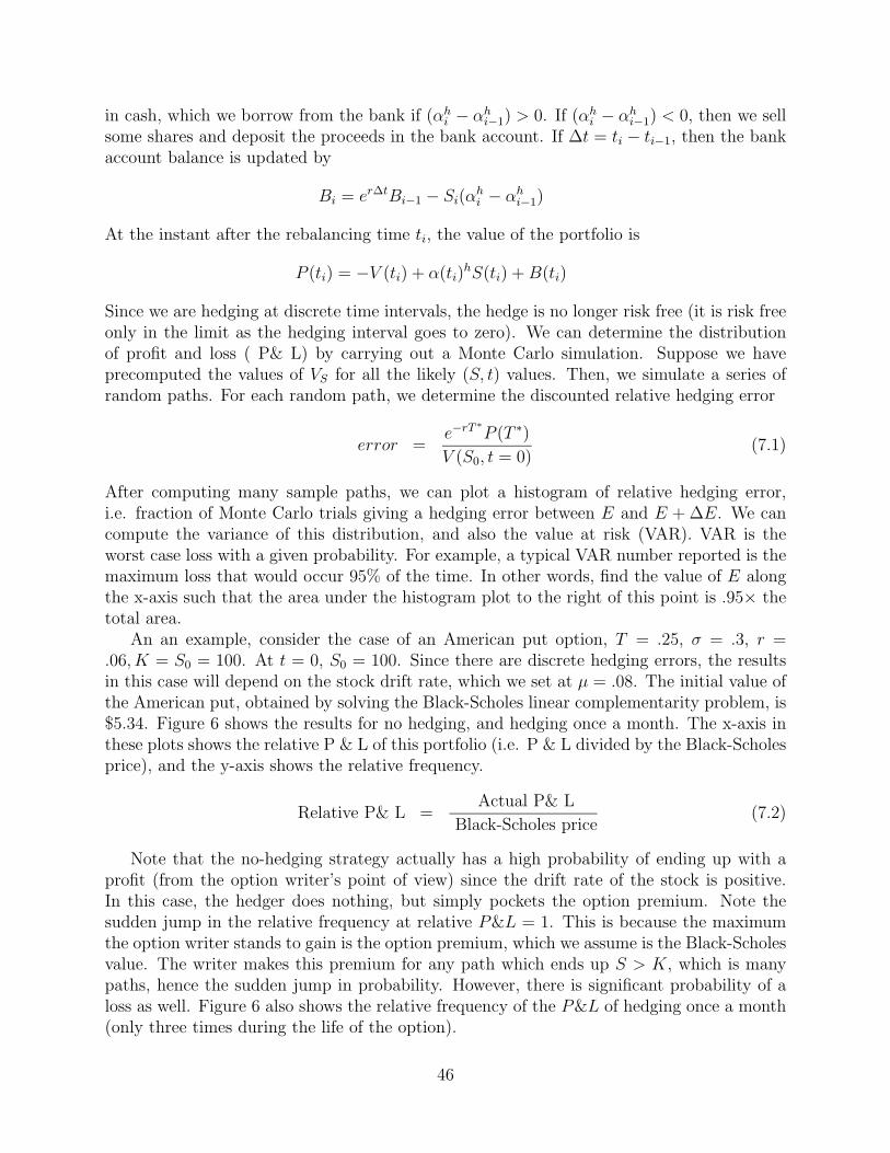
An an example, consider the case of an American put option, T = .25, σ = .3, r =.06, K = S0 = 100. At t = 0, S0 = 100. Since there are discrete hedging errors, the resultsin this case will depend on the stock drift rate, which we set at µ = .08. The initial value ofthe American put, obtained by solving the Black-Scholes linear complementarity problem, is$5.34. Figure 6 shows the results for no hedging, and hedging once a month. The x-axis inthese plots shows the relative P & L of this portfolio (i.e. P & L divided by the Black-Scholesprice), and the y-axis shows the relative frequency.
Relative P& L =Actual P& L
Black-Scholes price(7.2)
Note that the no-hedging strategy actually has a high probability of ending up with aprofit (from the option writer’s point of view) since the drift rate of the stock is positive.In this case, the hedger does nothing, but simply pockets the option premium. Note thesudden jump in the relative frequency at relative P&L = 1. This is because the maximumthe option writer stands to gain is the option premium, which we assume is the Black-Scholesvalue. The writer makes this premium for any path which ends up S > K, which is manypaths, hence the sudden jump in probability. However, there is significant probability of aloss as well. Figure 6 also shows the relative frequency of the P&L of hedging once a month(only three times during the life of the option).
46
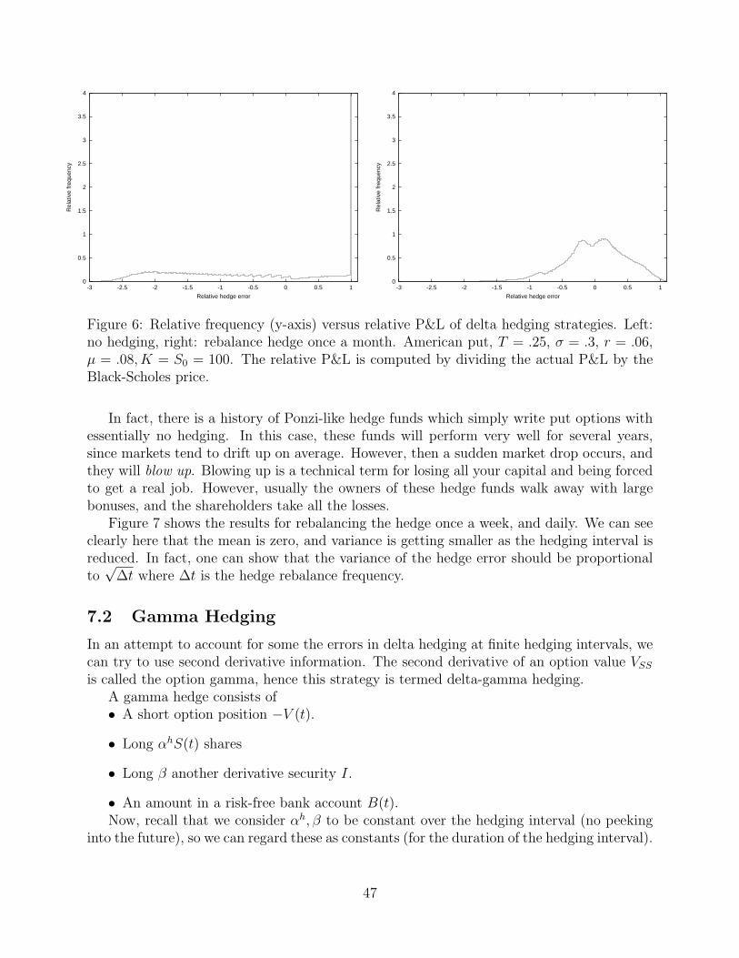
0
0.5
1
1.5
2
2.5
3
3.5
4
-3 -2.5 -2 -1.5 -1 -0.5 0 0.5 1
Rel
ativ
e fr
eque
ncy
Relative hedge error
0
0.5
1
1.5
2
2.5
3
3.5
4
-3 -2.5 -2 -1.5 -1 -0.5 0 0.5 1
Rel
ativ
e fr
eque
ncy
Relative hedge error
Figure 6: Relative frequency (y-axis) versus relative P&L of delta hedging strategies. Left:no hedging, right: rebalance hedge once a month. American put, T = .25, σ = .3, r = .06,µ = .08, K = S0 = 100. The relative P&L is computed by dividing the actual P&L by theBlack-Scholes price.
In fact, there is a history of Ponzi-like hedge funds which simply write put options withessentially no hedging. In this case, these funds will perform very well for several years,since markets tend to drift up on average. However, then a sudden market drop occurs, andthey will blow up. Blowing up is a technical term for losing all your capital and being forcedto get a real job. However, usually the owners of these hedge funds walk away with largebonuses, and the shareholders take all the losses.
Figure 7 shows the results for rebalancing the hedge once a week, and daily. We can seeclearly here that the mean is zero, and variance is getting smaller as the hedging interval isreduced. In fact, one can show that the variance of the hedge error should be proportionalto√
∆t where ∆t is the hedge rebalance frequency.
7.2 Gamma Hedging
In an attempt to account for some the errors in delta hedging at finite hedging intervals, wecan try to use second derivative information. The second derivative of an option value VSSis called the option gamma, hence this strategy is termed delta-gamma hedging.
A gamma hedge consists of• A short option position −V (t).
• Long αhS(t) shares
• Long β another derivative security I.
• An amount in a risk-free bank account B(t).Now, recall that we consider αh, β to be constant over the hedging interval (no peeking
into the future), so we can regard these as constants (for the duration of the hedging interval).
47
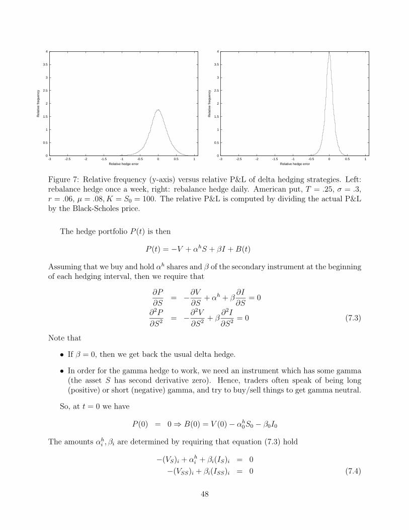
0
0.5
1
1.5
2
2.5
3
3.5
4
-3 -2.5 -2 -1.5 -1 -0.5 0 0.5 1
Rel
ativ
e fr
eque
ncy
Relative hedge error
0
0.5
1
1.5
2
2.5
3
3.5
4
-3 -2.5 -2 -1.5 -1 -0.5 0 0.5 1
Rel
ativ
e fr
eque
ncy
Relative hedge error
Figure 7: Relative frequency (y-axis) versus relative P&L of delta hedging strategies. Left:rebalance hedge once a week, right: rebalance hedge daily. American put, T = .25, σ = .3,r = .06, µ = .08, K = S0 = 100. The relative P&L is computed by dividing the actual P&Lby the Black-Scholes price.
The hedge portfolio P (t) is then
P (t) = −V + αhS + βI +B(t)
Assuming that we buy and hold αh shares and β of the secondary instrument at the beginningof each hedging interval, then we require that
∂P
∂S= −∂V
∂S+ αh + β
∂I
∂S= 0
∂2P
∂S2 = −∂2V
∂S2 + β∂2I
∂S2 = 0 (7.3)
Note that
• If β = 0, then we get back the usual delta hedge.
• In order for the gamma hedge to work, we need an instrument which has some gamma(the asset S has second derivative zero). Hence, traders often speak of being long(positive) or short (negative) gamma, and try to buy/sell things to get gamma neutral.
So, at t = 0 we have
P (0) = 0⇒ B(0) = V (0)− αh0S0 − β0I0
The amounts αhi , βi are determined by requiring that equation (7.3) hold
−(VS)i + αhi + βi(IS)i = 0
−(VSS)i + βi(ISS)i = 0 (7.4)
48
0
5
10
15
20
25
30
35
40
-3 -2.5 -2 -1.5 -1 -0.5 0 0.5 1
Rel
ativ
e fr
eque
ncy
Relative hedge error
0
5
10
15
20
25
30
35
40
-3 -2.5 -2 -1.5 -1 -0.5 0 0.5 1
Rel
ativ
e fr
eque
ncy
Relative hedge error
Figure 8: Relative frequency (y-axis) versus relative P&L of gamma hedging strategies.Left: rebalance hedge once a week, right: rebalance hedge daily. Dotted lines show the deltahedge for comparison. American put, T = .25, σ = .3, r = .06, µ = .08, K = 100, S0 = 100.Secondary instrument: European put option, same strike, T = .5 years. The relative P&Lis computed by dividing the actual P&L by the Black-Scholes price.
The bank account balance is then updated at each hedging time ti by
Bi = er∆tBi−1 − Si(αhi − αhi−1)− Ii(βi − βi−1)
We will consider the same example as we used in the delta hedge example. For anadditional instrument, we will use a European put option written on the same underlyingwith the same strike price and a maturity of T=.5 years.
Figure 8 shows the results of gamma hedging, along with a comparison on delta hedging.In principle, gamma hedging produces a smaller variance with less frequent hedging. How-ever, we are exposed to more model error in this case, since we need to be able to computethe second derivative of the theoretical price.
8 Jump Diffusion
Recall that if
dS = µSdt+ σS dZ (8.1)
then from Ito’s Lemma we have
d[logS] = [µ− σ2
2] dt+ σ dZ. (8.2)
49
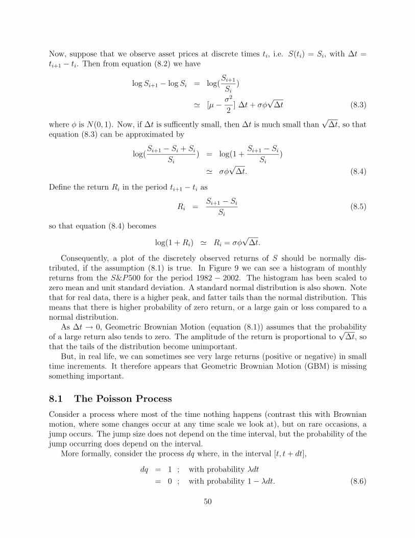
Now, suppose that we observe asset prices at discrete times ti, i.e. S(ti) = Si, with ∆t =ti+1 − ti. Then from equation (8.2) we have
logSi+1 − logSi = log(Si+1
Si)
' [µ− σ2
2] ∆t+ σφ
√∆t (8.3)
where φ is N(0, 1). Now, if ∆t is sufficently small, then ∆t is much small than√
∆t, so thatequation (8.3) can be approximated by
log(Si+1 − Si + Si
Si) = log(1 +
Si+1 − SiSi
)
' σφ√
∆t. (8.4)
Define the return Ri in the period ti+1 − ti as
Ri =Si+1 − Si
Si(8.5)
so that equation (8.4) becomes
log(1 +Ri) ' Ri = σφ√
∆t.
Consequently, a plot of the discretely observed returns of S should be normally dis-tributed, if the assumption (8.1) is true. In Figure 9 we can see a histogram of monthlyreturns from the S&P500 for the period 1982 − 2002. The histogram has been scaled tozero mean and unit standard deviation. A standard normal distribution is also shown. Notethat for real data, there is a higher peak, and fatter tails than the normal distribution. Thismeans that there is higher probability of zero return, or a large gain or loss compared to anormal distribution.
As ∆t → 0, Geometric Brownian Motion (equation (8.1)) assumes that the probabilityof a large return also tends to zero. The amplitude of the return is proportional to
√∆t, so
that the tails of the distribution become unimportant.But, in real life, we can sometimes see very large returns (positive or negative) in small
time increments. It therefore appears that Geometric Brownian Motion (GBM) is missingsomething important.
8.1 The Poisson Process
Consider a process where most of the time nothing happens (contrast this with Brownianmotion, where some changes occur at any time scale we look at), but on rare occasions, ajump occurs. The jump size does not depend on the time interval, but the probability of thejump occurring does depend on the interval.
More formally, consider the process dq where, in the interval [t, t+ dt],
dq = 1 ; with probability λdt
= 0 ; with probability 1− λdt. (8.6)
50
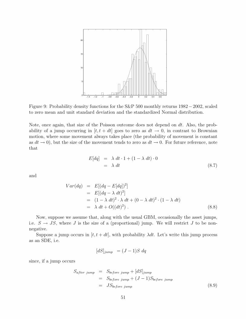
−1.4 −1.2 −1 −0.8 −0.6 −0.4 −0.2 0 0.2 0.4 0.60
5
10
15
20
Figure 9: Probability density functions for the S&P 500 monthly returns 1982−2002, scaledto zero mean and unit standard deviation and the standardized Normal distribution.
Note, once again, that size of the Poisson outcome does not depend on dt. Also, the prob-ability of a jump occurring in [t, t + dt] goes to zero as dt → 0, in contrast to Brownianmotion, where some movement always takes place (the probability of movement is constantas dt→ 0), but the size of the movement tends to zero as dt→ 0. For future reference, notethat
E[dq] = λ dt · 1 + (1− λ dt) · 0= λ dt (8.7)
and
V ar(dq) = E[(dq − E[dq])2]
= E[(dq − λ dt)2]
= (1− λ dt)2 · λ dt+ (0− λ dt)2 · (1− λ dt)= λ dt+O((dt)2) . (8.8)
Now, suppose we assume that, along with the usual GBM, occasionally the asset jumps,i.e. S → JS, where J is the size of a (proportional) jump. We will restrict J to be non-negative.
Suppose a jump occurs in [t, t + dt], with probability λdt. Let’s write this jump processas an SDE, i.e.
[dS]jump = (J − 1)S dq
since, if a jump occurs
Safter jump = Sbefore jump + [dS]jump
= Sbefore jump + (J − 1)Sbefore jump
= JSbefore jump (8.9)
51
which is what we want to model. So, if we have a combination of GBM and a rare jumpevent, then
dS = µS dt+ σS dZ + (J − 1)S dq (8.10)
Assume that the jump size has some known probability density g(J), i.e. given that a jumpoccurs, then the probability of a jump in [J, J + dJ ] is g(J) dJ , and∫ +∞
−∞g(J) dJ =
∫ ∞0
g(J) dJ = 1 (8.11)
since we assume that g(J) = 0 if J < 0. For future reference, if f = f(J), then the expectedvalue of f is
E[f ] =
∫ ∞0
f(J)g(J) dJ . (8.12)
8.2 The Jump Diffusion Pricing Equation
Now, form the usual hedging portfolio
P = V − αS . (8.13)
Now, consider
[dP ]total = [dP ]Brownian + [dP ]jump (8.14)
where, from Ito’s Lemma
[dP ]Brownian = [Vt +σ2S2
2VSS]dt+ [V − αS](µS dt+ σS dZ) (8.15)
and, noting that the jump is of finite size,
[dP ]jump = [V (JS, t)− V (S, t)] dq − α(J − 1)S dq . (8.16)
If we hedge the Brownian motion risk, by setting α = VS, then equations (8.14-8.16) give us
dP = [Vt +σ2S2
2VSS]dt+ [V (JS, t)− V (S, t)]dq − VS(J − 1)S dq . (8.17)
So, we still have a random component (dq) which we have not hedged away. Let’s take theexpected value of this change in the portfolio, e.g.
E(dP ) = [Vt +σ2S2
2VSS]dt+ E[V (JS, t)− V (S, t)]E[dq]− VSSE[J − 1]E[dq](8.18)
where we have assumed that probability of the jump and the probability of the size of thejump are independent. Defining E(J − 1) = κ, then we have that equation (8.18) becomes
E(dP ) = [Vt +σ2S2
2VSS]dt+ E[V (JS, t)− V (S, t)]λ dt− VSSκλ dt . (8.19)
52
Now, we make a rather interesting assumption. Assume that an investor holds a diver-sified portfolio of these hedging portfolios, for many different stocks. If we make the ratherdubious assumption that these jumps for different stocks are uncorrelated, then the varianceof this portfolio of portfolios is small, hence there is little risk in this portfolio. Hence, theexpected return should be
E[dP ] = rP dt . (8.20)
Now, equating equations (8.19 and (8.20) gives
Vt +σ2S2
2VSS + VS[rS − Sκλ]− (r + λ)V + E[V (JS, t)]λ = 0 . (8.21)
Using equation (8.12) in equation (8.21) gives
Vt +σ2S2
2VSS + VS[rS − Sκλ]− (r + λ)V + λ
∫ ∞0
g(J)V (JS, t) dJ = 0 . (8.22)
Equation (8.22) is a Partial Integral Differential Equation (PIDE).A common assumption is to assume that g(J) is log normal,
g(J) =exp
(− (log(J)2−µ)
2γ2
)√
2πγJ. (8.23)
where, some algebra shows that
E(J − 1) = κ = exp(µ+ γ2/2)− 1 . (8.24)
Now, what about our dubious assumption that jump risk was diversifiable? In practice, wecan regard σ, µ, γ, λ as parameters, and fit them to observed option prices. If we do this,(see L. Andersen and J. Andreasen, Jump-Diffusion processes: Volatility smile fitting andnumerical methods, Review of Derivatives Research (2002), vol 4, pages 231-262), then wefind that σ is close to historical volatility, but that the fitted values of λ, µ are at odds withthe historical values. The fitted values seem to indicate that investors are pricing in largermore frequent jumps than has been historically observed. In other words, actual prices seemto indicate that investors do require some compensation for jump risk, which makes sense.In other words, these parameters contain a market price of risk.
Consequently, our assumption about jump risk being diversifiable is not really a problemif we fit the jump parameters from market (as opposed to historical) data, since the market-fitparameters will contain some effect due to risk preferences of investors.
9 Further Reading
• Peter Bernstein, Capital Ideas: the improbable origins of modern Wall street, The FreePress, New York, 1992.
53
• Peter Bernstein, Against the Gods: the remarkable story of risk, John Wiley, New York,1998, ISBN 0-471-29563-9.
• Boyle, Broadie, Glassermman, Monte Carlo methods for security pricing, J. Econ. Dyn.Con., 21:1267-1321 (1997)
• A. Dixit and R. Pindyck, Investment under uncertainty, Princeton University Press,1994.
• John Hull, Options, futures and other derivatives, Prentice-Hall, 1997, ISBN 0-13-186479-3.
• Burton Malkeil, A random walk down Wall Street, W.W. Norton, New York, 1999,ISBN 0-393-32040-5.
• D. Tavella and C. Randall, Pricing Financial Instruments: the Finite Difference Method,Wiley, 2000, ISBN 0-471-19760-2.
• N. Taleb, Fooled by Randomness, Texere, 2001, ISBN 1-58799-071-7. 21:1267-1321(1997)
• N. Taleb, Dynamic Hedging, Wiley, 1997, ISBN 0-471-15280-3.
• Lenos Triegeorgis, Real Options: Managerial Flexibility and Strategy for Resource Al-location, MIT Press, 1996, ISBN 0-262-20102-X.
• P. Wilmott, S. Howison, J. Dewynne, The mathematics of financial derivatives: Astudent introduction, Cambridge, 1997, ISBN 0-521-49789-2.
• Paul Wilmott, Derivatives: the theory and practice of financial engineering, Wiley,1998, ISBN 0-471-983-66-7.
An interesting web site on Real Options is at www.real-options.com.
54