an introduction to macroeconometrics: vec and var models prepared by vera tabakova, east carolina...
TRANSCRIPT

Chapter 13
An Introduction to Macroeconometrics: VEC and VAR Models
Prepared by Vera Tabakova, East Carolina University

Chapter 13: An Introduction to Macroeconometrics: VEC and VAR Models
13.1 VEC and VAR Models
13.2 Estimating a Vector Error Correction model
13.3 Estimating a VAR Model
13.4 Impulse Responses and Variance Decompositions
Slide 13-2Principles of Econometrics, 3rd Edition

Chapter 13: An Introduction to Macroeconometrics: VEC and VAR Models
Slide 13-3Principles of Econometrics, 3rd Edition
(13.1a)
(13.1b)
210 11 , ~ (0, )y y
t t t t yy x e e N
220 21 , ~ (0, )x x
t t t t xx y e e N

13.1 VEC and VAR Models
Slide 13-4Principles of Econometrics, 3rd Edition
(13.2)
(13.3)
10 11 1 12 1
20 21 1 22 1
yt t t t
xt t t t
y y x v
x y x v
11 1 12 1
21 1 22 1
yt t t t
xt t t t
y y x v
x y x v

13.1 VEC and VAR Models
Slide 13-5Principles of Econometrics, 3rd Edition
(13.4)
(13.5a)
0 1t t ty x e
10 11 1 0 1 1
20 21 1 0 1 1
( )
( )
yt t t t
xt t t t
y y x v
x y x v
13.1 VEC and VAR Models
Slide 13-6Principles of Econometrics, 3rd Edition
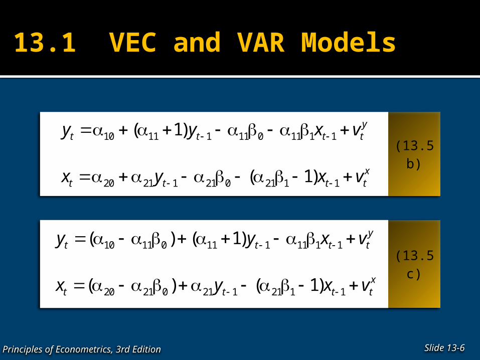
(13.5b)
(13.5c)
10 11 1 11 0 11 1 1
20 21 1 21 0 21 1 1
( 1)
( 1)
yt t t t
xt t t t
y y x v
x y x v
10 11 0 11 1 11 1 1
20 21 0 21 1 21 1 1
( ) ( 1)
( ) ( 1)
yt t t t
xt t t t
y y x v
x y x v
13.2 Estimating a Vector Error Correction Model
Slide 13-7Principles of Econometrics, 3rd Edition
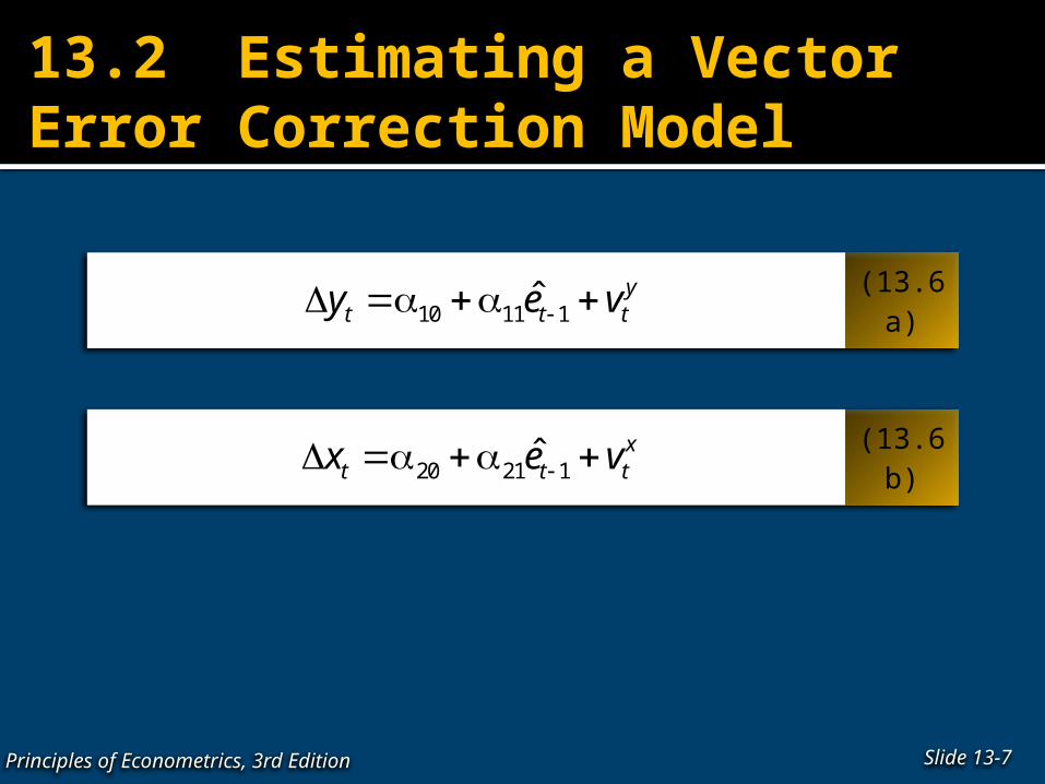
(13.6a)
(13.6b)
10 11 1ˆ yt t ty e v
20 21 1ˆ xt t tx e v

13.2.1 Example
Figure 13.1 Real Gross Domestic Products (GDP)
Slide 12-8Principles of Econometrics, 3rd Edition
13.2.1 Example
Slide 13-9Principles of Econometrics, 3rd Edition
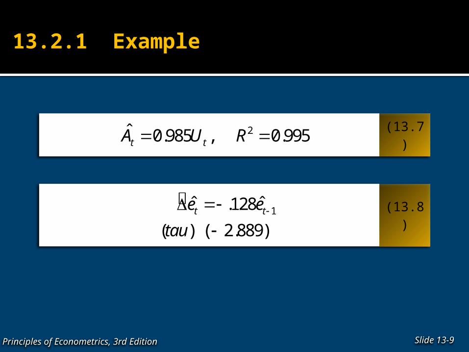
(13.7)
(13.8)
2ˆ 0.985 , 0.995t tA U R
1ˆ ˆ.128
( ) ( 2.889)t te e
tau

13.2.1 Example
Slide 13-10Principles of Econometrics, 3rd Edition
(13.9)
1
1
ˆ0.492 0.099
( ) (2.077)
ˆ0.510 0.030
( ) (0.789)
t t
t t
A e
t
U e
t

13.3 Estimating a VAR Model
Figure 13.2 Real GDP and the Consumer Price Index (CPI)
Slide 12-11Principles of Econometrics, 3rd Edition

13.3 Estimating a VAR Model
Slide 13-12Principles of Econometrics, 3rd Edition
(13.10)1
ˆ 1.631 0.623
ˆ ˆ0.009
( ) ( 0.977)
t t t
t t
e G P
e e
tau
13.3 Estimating a VAR Model
Slide 13-13Principles of Econometrics, 3rd Edition
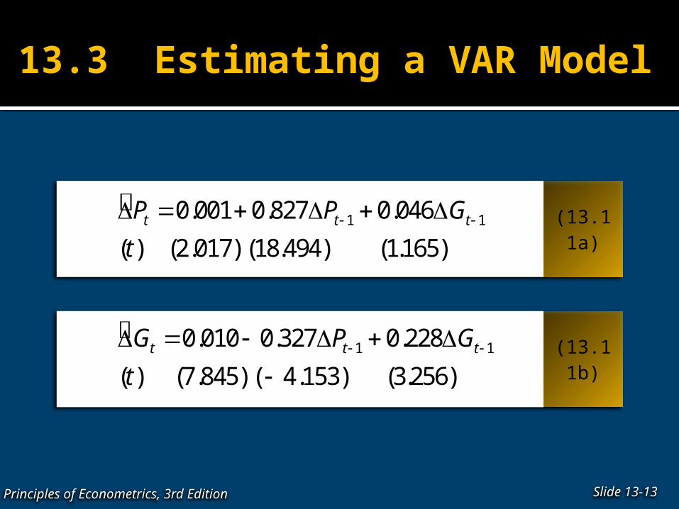
(13.11a)
1 10.001 0.827 0.046
( ) (2.017) (18.494) (1.165) t t tP P G
t
(13.11b)
1 10.010 0.327 0.228
( ) (7.845) ( 4.153) (3.256) t t tG P G
t

13.4 Impulse Responses and Variance Decompositions 13.4.1 Impulse Response Functions
13.4.1a The Univariate Case
The series is subject it to a shock of size ν in period 1.
Slide 13-14Principles of Econometrics, 3rd Edition
1t t ty y v
1 0 1
2 1
23 2 1
2
1,
2,
3, ( )
...
the shock is , , ,
t y y v v
t y y v
t y y y v
v v v
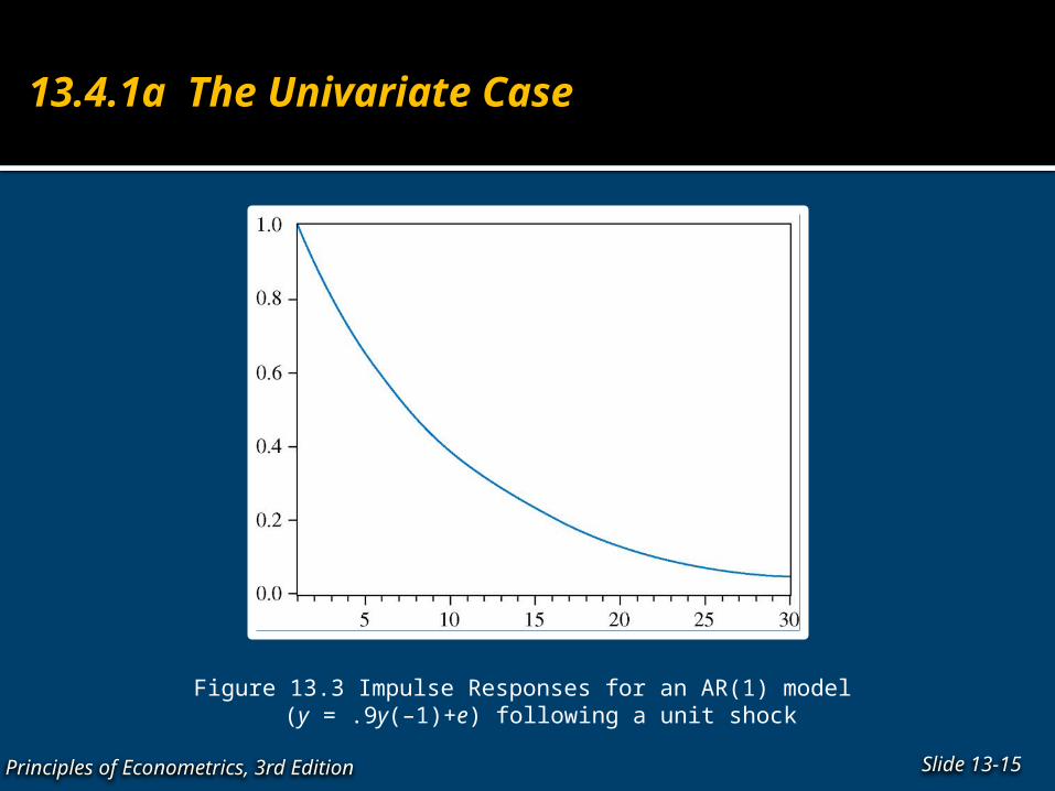
13.4.1a The Univariate Case
Figure 13.3 Impulse Responses for an AR(1) model (y = .9y(–1)+e) following a unit shock
Slide 13-15Principles of Econometrics, 3rd Edition

13.4.1b The Bivariate Case
Slide 13-16Principles of Econometrics, 3rd Edition
(13.12)
10 11 1 12 1
20 21 1 22 1
yt t t t
xt t t t
y y x v
x y x v
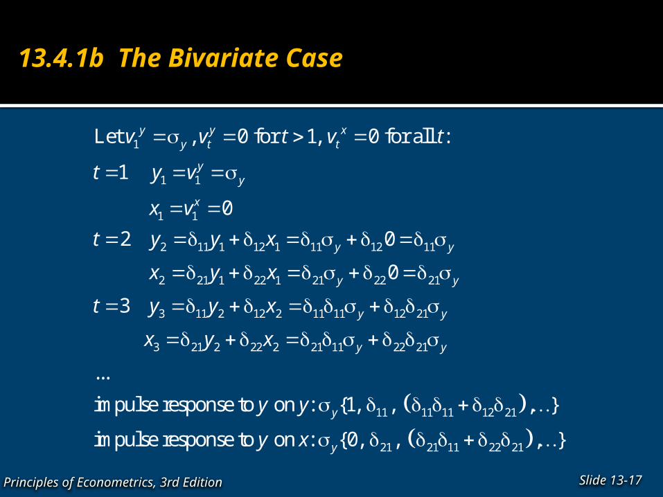
13.4.1b The Bivariate Case
Slide 13-17Principles of Econometrics, 3rd Edition
1
1 1
1 1
2 11 1 12 1 11 12 11
2 21 1 22 1 21 22 21
3 11 2 12 2 11 11 12 21
Let , 0 for 1, 0 for all :
1
0
2 0
0
3
y y xy t t
yy
x
y y
y y
y y
v v t v t
t y v
x v
t y y x
x y x
t y y x
3 21 2 22 2 21 11 22 21
11 11 11 12 21
21 21 11 22 21
...
impulse response to on : {1, , , }
impulse response to on : {0, , , }
y y
y
y
x y x
y y
y x
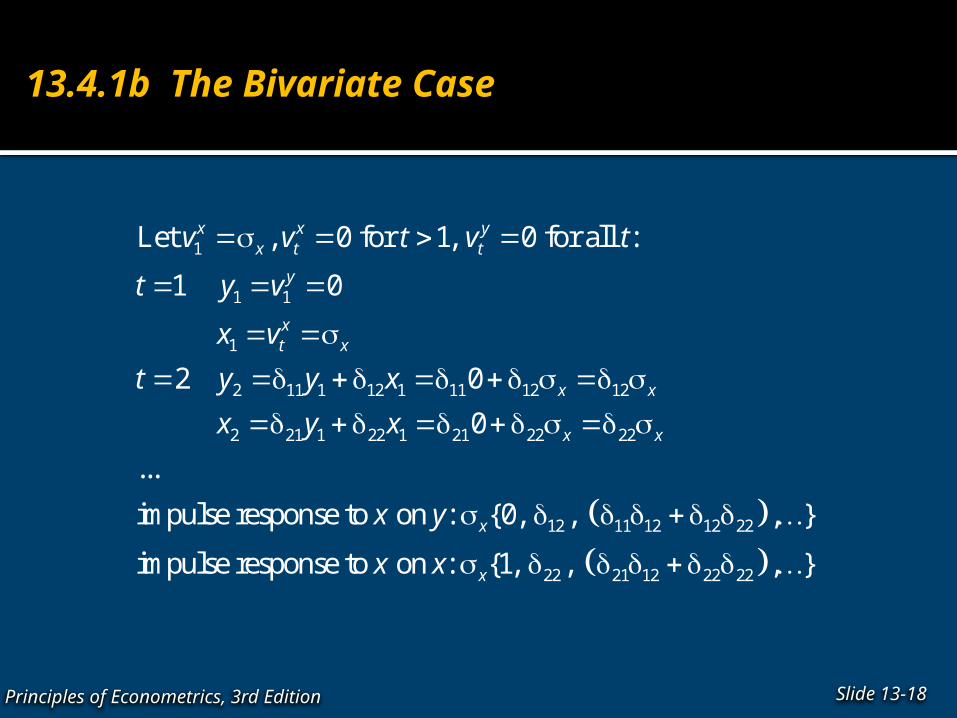
13.4.1b The Bivariate Case
Slide 13-18Principles of Econometrics, 3rd Edition
1
1 1
1
2 11 1 12 1 11 12 12
2 21 1 22 1 21 22 22
12
Let , 0 for 1, 0 for all :
1 0
2 0
0
...
impulse response to on : {0, ,
x x yx t t
y
xt x
x x
x x
x
v v t v t
t y v
x v
t y y x
x y x
x y
11 12 12 22
22 21 12 22 22
, }
impulse response to on : {1, , , }xx x
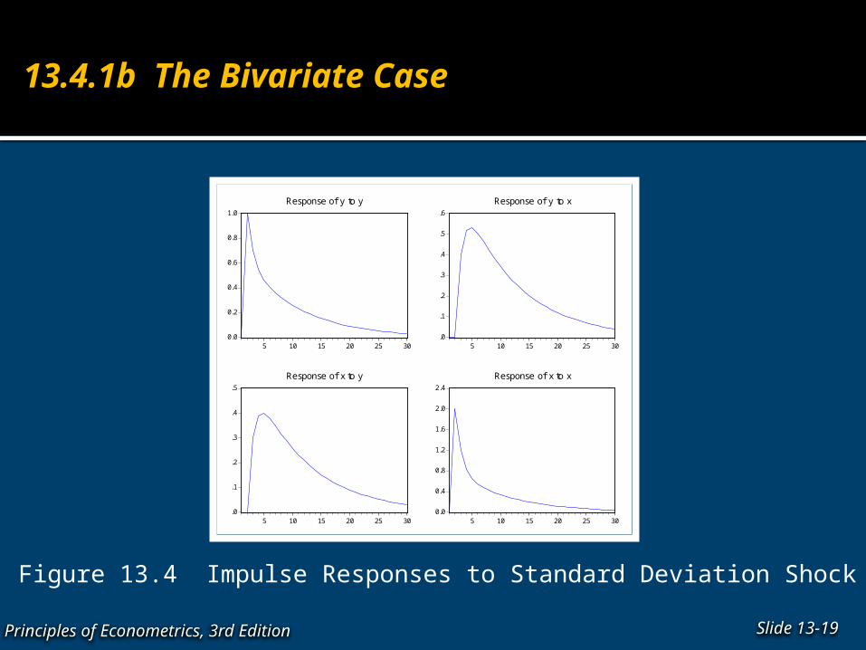
13.4.1b The Bivariate Case
Figure 13.4 Impulse Responses to Standard Deviation Shock
Slide 13-19Principles of Econometrics, 3rd Edition
0.0
0.2
0.4
0.6
0.8
1.0
5 10 15 20 25 30
Response of y to y
.0
.1
.2
.3
.4
.5
.6
5 10 15 20 25 30
Response of y to x
.0
.1
.2
.3
.4
.5
5 10 15 20 25 30
Response of x to y
0.0
0.4
0.8
1.2
1.6
2.0
2.4
5 10 15 20 25 30
Response of x to x

13.4.2 Forecast Error Variance Decompositions
13.4.2a The Univariate Case
Slide 13-20Principles of Econometrics, 3rd Edition
1
1 1
1 1 1 1
22 1 2 1 2
22 2 2 1 2
[ ]
[ ]
[ ] [ ( ) ]
[ ]
t t t
Ft t t t
t t t t t t
Ft t t t t t t t t
t t t t t t t
y y v
y E y v
y E y y y v
y E y v E y v v y
y E y y y v v

13.4.2 Forecast Error Variance Decompositions
13.4.2b The Bivariate Case
Slide 13-21Principles of Econometrics, 3rd Edition
1 11 12 1 11 12
1 21 22 1 21 22
21 1 1 1 1
21 1 1 1 1
[ ]
[ ]
[ ] ; var( )
[ ] ; var( )
F yt t t t t t t
F xt t t t t t t
y y yt t t t y
x x xt t t t x
y E y x v y x
x E y x v y x
FE y E y v FE
FE x E x v FE

13.4.2 Forecast Error Variance Decompositions
13.4.2b The Bivariate Case
Slide 13-22Principles of Econometrics, 3rd Edition
2 11 1 12 1 2
11 11 12 1 12 21 22 1 2
11 11 12 12 21 22
[ ]
[ ]
F yt t t t t
y x yt t t t t t t t
t t t t
y E y x v
E y x v y x v v
y x y x
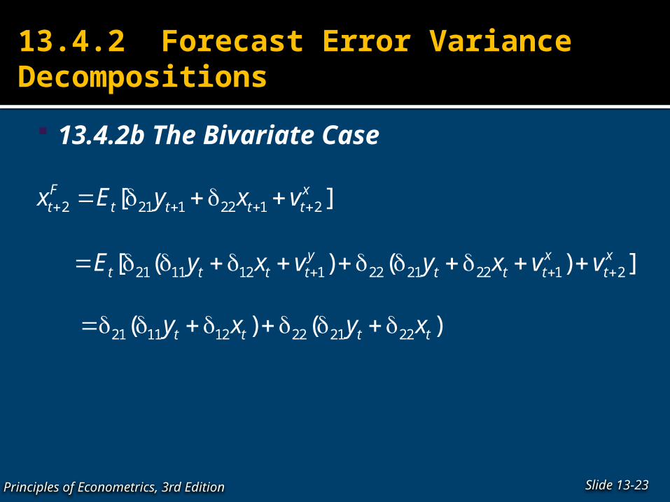
13.4.2 Forecast Error Variance Decompositions
13.4.2b The Bivariate Case
Slide 13-23Principles of Econometrics, 3rd Edition
2 21 1 22 1 2
21 11 12 1 22 21 22 1 2
21 11 12 22 21 22
[ ]
[ ( ) ( ) ]
( ) ( )
F xt t t t t
y x xt t t t t t t t
t t t t
x E y x v
E y x v y x v v
y x y x
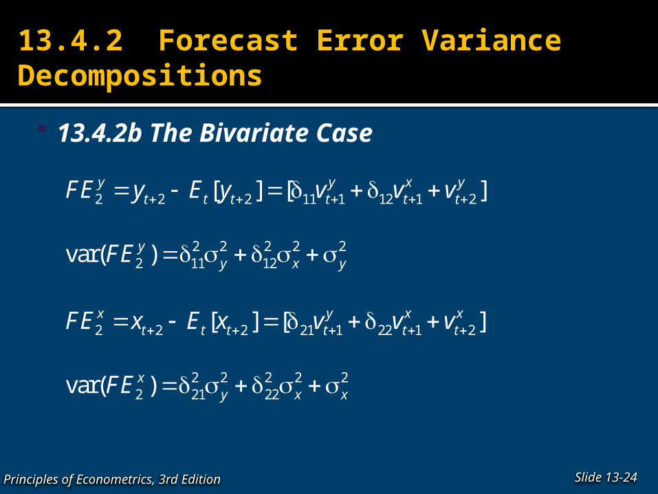
13.4.2 Forecast Error Variance Decompositions
13.4.2b The Bivariate Case
Slide 13-24Principles of Econometrics, 3rd Edition
2 2 2 11 1 12 1 2
2 2 2 2 22 11 12
2 2 2 21 1 22 1 2
2 2 2 2 22 21 22
[ ] [ ]
var( )
[ ] [ ]
var( )
y y x yt t t t t t
yy x y
x y x xt t t t t t
xy x x
FE y E y v v v
FE
FE x E x v v v
FE

13.4.2 Forecast Error Variance Decompositions
13.4.2c The General Case
The example above assumes that x and y are not contemporaneously related and that the shocks are uncorrelated. There is no identification problem and the generation and interpretation of the impulse response functions and decomposition of the forecast error variance are straightforward. In general, this is unlikely to be the case. Contemporaneous interactions and correlated errors complicate the identification of the nature of shocks and hence the interpretation of the impulses and decomposition of the causes of the forecast error variance.
Slide 13-25Principles of Econometrics, 3rd Edition

Keywords
Slide 13-26Principles of Econometrics, 3rd Edition
Dynamic relationships Error Correction Forecast Error Variance
Decomposition Identification problem Impulse Response Functions VAR model VEC Model

Chapter 13 Appendix
Slide 13-27Principles of Econometrics, 3rd Edition
Appendix 13A The Identification Problem

Appendix 13A The Identification Problem
Principles of Econometrics, 3rd Edition Slide 13-28
(13A.1)1 1 1 2 1
2 3 1 4 1
yt t t t t
xt t t t t
y x y x e
x y y x e
1 2 11
3 4 12
1
1
yt t t
xt t t
y y e
x x e
1 21
3 42
1; ;
1
ytxt
eB A E
e
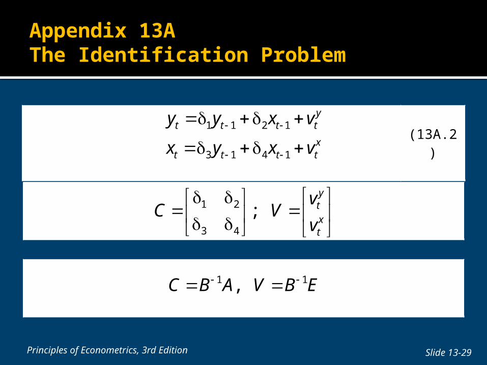
Appendix 13A The Identification Problem
Principles of Econometrics, 3rd Edition Slide 13-29
(13A.2)1 1 2 1
3 1 4 1
yt t t t
xt t t t
y y x v
x y x v
1 2
3 4
; ytxt
vC V
v
1 1, C B A V B E