An introduction to semi-Lagrangian methods III

Luca Bonaventura

Dipartimento di Matematica

“F. Brioschi”, Politecnico di Milano

MOX – Modeling and Scientific Computing Laboratory

Sapienza SL workshop 2011

The SL success storyThe SL success story

EECMWF forecast for today: made possible by SL methods

OutlineOutline

•From scalar advection to realistic transport models: need for mass conservative semi-Lagrangian methods

•Identify typical regimes for convenient application of SL to more complex fluid dynamics problems: NWP and the SL success story

•Some examples of other applications to environmental modeling

References on SL and alike References on SL and alike

Textbooks: Falcone Ferretti: to appearDurran, Quarteroni-Valli

Review papers: Staniforth and Coté, MWR 119 1991 Morton, SIAM J. Num. An. 1998 Ewing and Wang, J. Comp. Appl.Math. 2001 L.B., ETH Zurich ERCOFTAC 2004 lecture

notes (http://www1.mate.polimi.it/~bonavent)

The model problem The model problem

€

Dc

Dt=

∂c

∂t+ u(x, t) • ∇c = 0

c(x,0) = c0(x) x∈Rd

)),,0;((),0;(

)),0;((),( 0

tttdt

d

tctc

xXuxX

xXx

Representation formula for exact solution

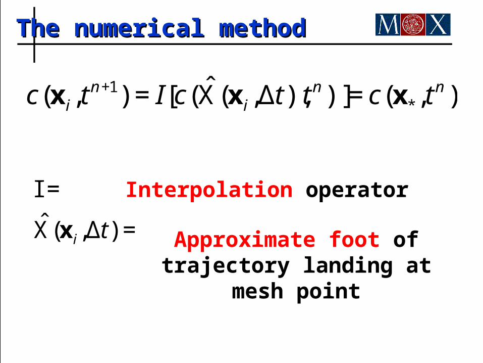
The numerical methodThe numerical method

€

c(x i, tn+1) = I[c( ˆ X (x i,Δt), t

n )] = c(x*, tn )

Interpolation operator

€

I =

ˆ X (x i,Δt) = Approximate foot of trajectory landing at mesh point

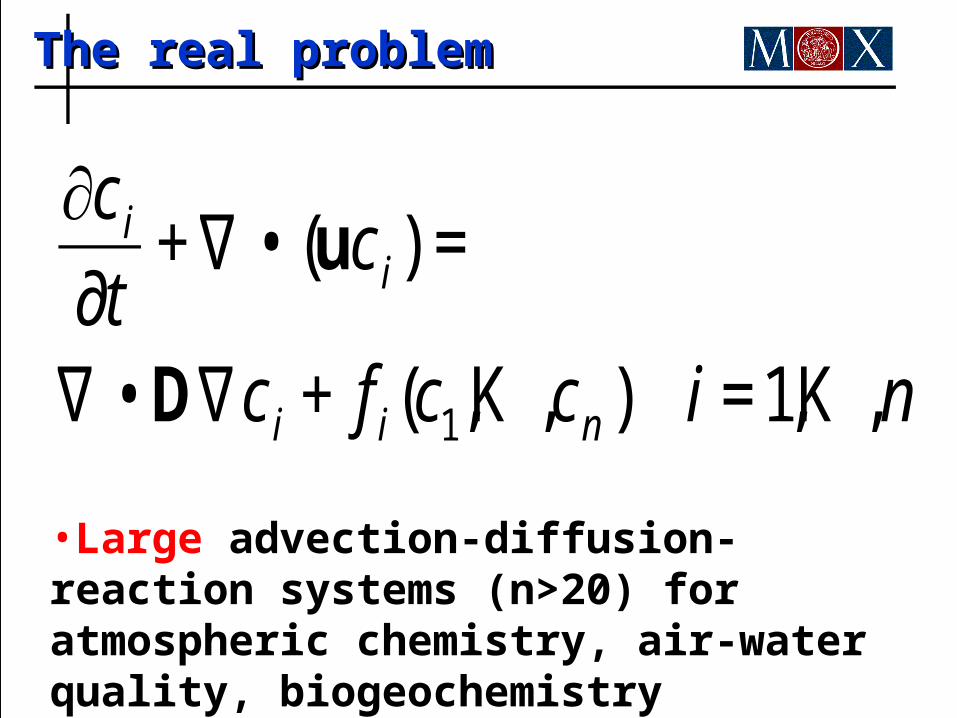
The real problemThe real problem

€

∂c i∂t

+∇ • (uc i) =

∇ • D∇c i + f i(c1,K ,cn ) i =1,K ,n

•Large advection-diffusion-reaction systems (n>20) for atmospheric chemistry, air-water quality, biogeochemistry

Example: air pollution modelExample: air pollution model

25 chemical reaction among 20 chemical species with very different reaction rates (stiff problem)

Computational requirementsComputational requirements

•High order accuracy, positivity preservation

•Fully multidimensional numerical methods

•Efficiency: standard explicit time discretization often have restrictive CFL stability conditions

•Mass conservation

Mass conservation issue for SL Mass conservation issue for SL

1InterpolationD test

Linear Quadratic Spline

Final/initial mass ratio

1.00002384 1.00293481 1.00027871

2D Interpolation

Linear Cubic, tr. I order trajectories

Cubic, II order trajectories

Final/initial mass ratio

0.7668 0.8828 1.1059

One dimensional test

Two dimensional test

Conservative SL : remappingConservative SL : remapping

0Dt

Dc

dxcdxc nn 1

SL conservative methods based on remapping: Laprise 1995, Machenhauer 1997, Nair 2002, Zerroukat and Staniforth 2003, Behrens and Menstrup 2004

Flux form SL methods, IFlux form SL methods, I

dcdtdxcdxctn

tn

nn

)1(

1 nu

0)(

ct

cu

dtd

ddcFtA

n

nu

)()u,,(

)(n)1(

Fdcdttn

tn

u

SL flux form conservative methods:

Lin Rood 1996; Fey 1998; Frolkovic 2002; B., Restelli Sacco 2006

Flux form SL methods, IIFlux form SL methods, II

Flux form SL methods, resultsFlux form SL methods, results

Advection test with monotonic (a) SLDG scheme, (b) conventional monotonic DG, (c) exact solution (Restelli Sacco B. JCP 2006)

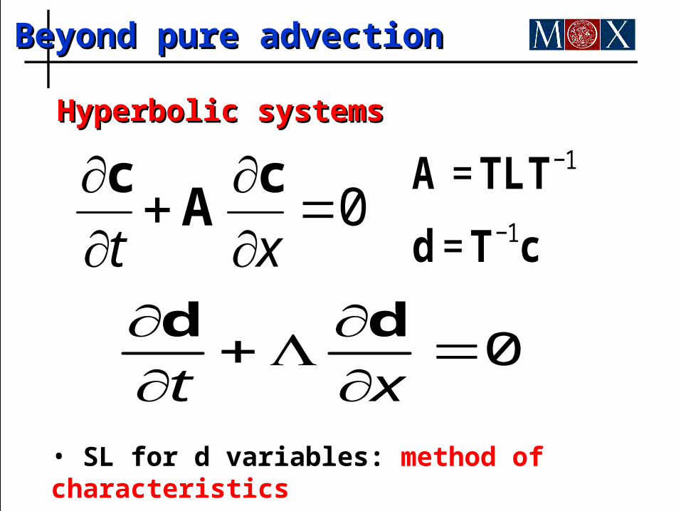
Beyond pure advectionBeyond pure advection

0

xt

cA

c

€

A = TLT−1

d = T−1c

0

xt

dd

• SL for d variables: method of characteristics

Hyperbolic systemsHyperbolic systems

Model problemModel problem

• Shallow water equations (2D Euler)

€

c =T

h, u[ ]

€

∂h∂t

+ u∂h

∂x+ h

∂u

∂x= 0

∂u

∂t+ u

∂u

∂x+ g

∂h

∂x= 0

€

A =u h

g u

⎡

⎣ ⎢

⎤

⎦ ⎥

Hydrodynamic regimesHydrodynamic regimes

€

u

gh≈1

€

u

gh<<1

Critical: large Froude/Mach numbers

Subcritical: small Froude/Mach numbers

Flow along characteristics,

discontinuous solutions

Flow along streamlines,

continuous solutions

€

Dh

Dt= −h

∂u

∂xDu

Dt= −g

∂h

∂x

From SL to SISLFrom SL to SISL

€

hin+1 − h*

n

Δt= −hi

n ∂un+1

∂xi

uin+1 − u*

n

Δt= −g

∂hn+1

∂xi

•Use advective form and apply SL + semi-implicit treatment of RHS

€

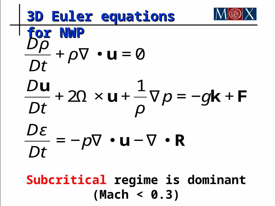
Dρ

Dt+ ρ∇ • u = 0

Du

Dt+ 2Ω × u +

1

ρ∇p = −gk + F

Dε

Dt= −p∇ • u −∇ • R

3D Euler equations for NWP3D Euler equations for NWP

Subcritical regime is dominant (Mach < 0.3)

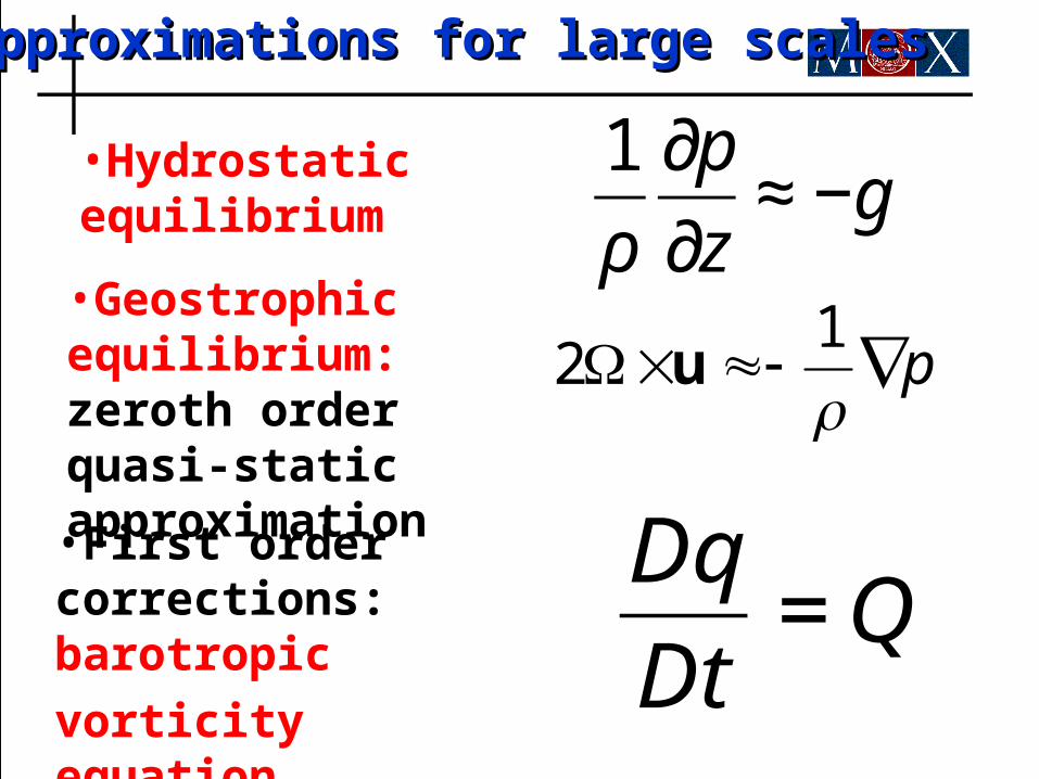
Approximations for large scalesApproximations for large scales

•Hydrostatic equilibrium

€

1

ρ

∂p

∂z≈ −g

•Geostrophic equilibrium: zeroth order quasi-static approximation

p1

2 u

•First order corrections: barotropic

vorticity equation

€

Dq

Dt=Q

The birth of NWP (1950)The birth of NWP (1950)

The birth of SL (1963) The birth of SL (1963)

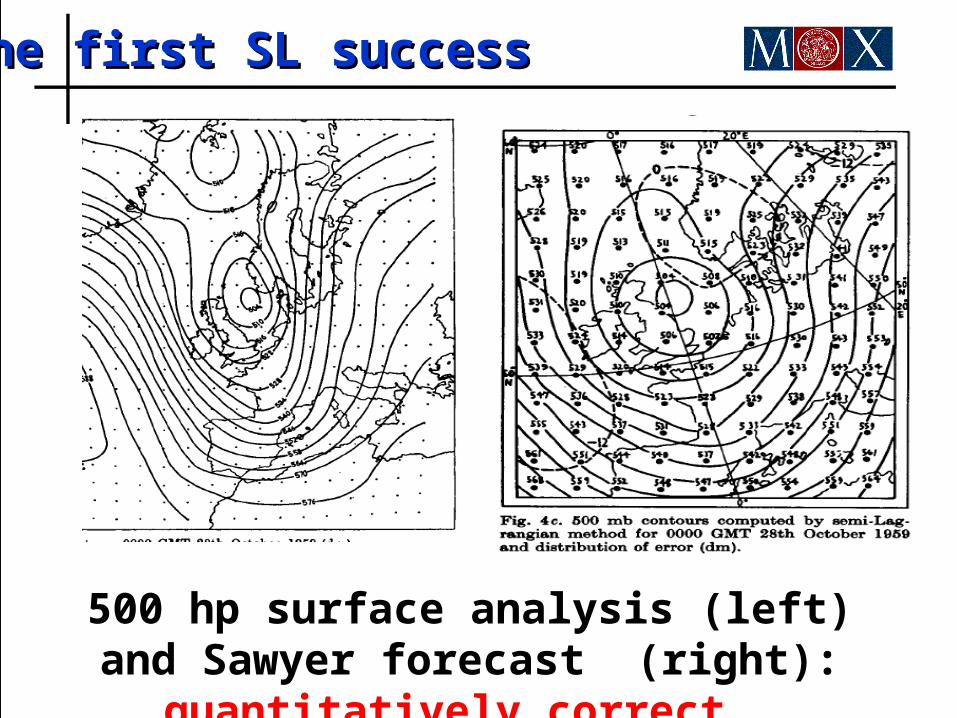
The first SL success The first SL success

500 hp surface analysis (left) and Sawyer forecast (right): quantitatively correct……

The first SL success The first SL success

…..at much lower computational cost

The SL success storyThe SL success story

Probabilistic forecast (EPS): average and standard deviations over 50 independent runs

Environmental applicationsEnvironmental applications

•Advection dominated, subcritical flows: river hydraulics, coastal modelling, high resolution atmospheric modeling

•Long time range simulations: need for maximum efficiency

•Wide range of different flow velocities: small portion of computational domain can restrict time step for standard explicit methods

River hydraulicsRiver hydraulics

Correct profiles for various regimes of channel flow achieved at high Courant numbers

River hydraulics (1.5D)River hydraulics (1.5D)

Flood prediction for the Adige river (De Ponti, Rosatti, B., Garegnani, IJNMF 2011)

River hydraulicsRiver hydraulics

Sediment transport in a curved channel (Rosatti, Chemotti,B. IJNMF 2005)

Coastal hydrodynamics (2-3D) Coastal hydrodynamics (2-3D)

•Venice Lagoon

•Dx=50 m,Dt=600 s

•Typical velocities: 0.1-1.0 m/s

• Complex geometry, need for appropriate trajectory computation

Coastal hydrodynamics (2-3D)Coastal hydrodynamics (2-3D)

High water prediction for the Venice lagoon

Nonhydrostatic flowsNonhydrostatic flows

•Idealized Foehn in a stratified atmosphere

•Dx = 2000 m, Dz = 200 m, Dt =30 s

•Semi-Lagrangian semi-implicit method (B., JCP 2000)

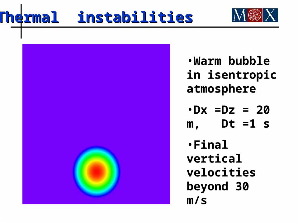
Thermal instabilitiesThermal instabilities

•Warm bubble in isentropic atmosphere

•Dx =Dz = 20 m, Dt =1 s

•Final vertical velocities beyond 30 m/s

Computational gainsComputational gains

CPU time for 1 hour

CPU time for SI solver

COMM time for SI solver

CPU time for advection

COMM time for advection

SE

328 91 13.4 156 40.8

SI Z

207 119 13.4 65.4 7.4

CPU times in seconds, comparison with split-explicit method, 3D gravity wave test case, 180*180*40 gridpoints (B., Cesari, Nuovo Cimento, 2005)

ConclusionsConclusions

•Semi-Lagrangian methods: an accurate and efficient method for subcritical flows

•NWP: almost ideal application area

•Wide range of applications to environmental modeling