An Introduction to Viscosity Solutions:

theory, numerics and applications

M. Falcone

Dipartimento di Matematica

OPTPDE-BCAM Summer School

”Challenges in Applied Control and Optimal Design”

July 4-8, 2011, Bilbao – Lecture 2/4

OUTLINE OF THE COURSE:

• Lecture 1: Introduction to viscosity solutions

• Lecture 2: Approximation schemes for viscosity solutions

• Lecture 3: Approximation of optimal control problems via DP

• Lecture 4: Efficient methods and perspectives

OUTLINE OF THIS LECTURE:

Approximation schemes for viscosity solutions

• Approximation schemes for 1st order PDEs

• Finite difference

• A general convergence results for monotone schemes

• Semi-Lagrangian schemes

• Convergence for SL schemes

• HJPACK: a public domain library

Computing viscosity solutions

Viscosity solutions are typically uniformly continuous and bounded.

As we will see also discontinuous solution can be considered in

the framework of this theory.

This means that the numerical methods should be able to re-

construct kinks in the solution and, possibly, jumps.

Computing viscosity solutions

The main goals are:

• consistency

• stability

• convergence

• small ”numerical viscosity”

Moreover, the schemes should also be able to compute solutions

after the onset of singularities/jumps without producing spurious

oscillations.

Model problem: 1st order PDEs

Let us consider the evolutive equation in R.

vt + H(vx) = 0 in R × (0, T),

v(x,0) = v0(x) in R(HJ)

where H(·) is convex.

We know the relation between (HJ) and the associated conser-

vation law. Roughly speaking, the entropy solution of (CL) is

the ”derivative” of the viscosity solution.

Typical approximation methods in this framework

Due to the hyperbolic nature of these equations and to their

nonlinearity the most popular methods are

• Finite Differences schemes

• Semi-Lagrangian schemes

• Discontinuous Galerkin methods

We restrict our presentation to the first two.

Finite Difference schemes

An important source of FD approximation schemes is the huge

collection of approximation schemes developed for conservation

laws.

In fact, we can always integrate in space a scheme for (CL) and

obtain a suitable scheme for (HJ).

The general discrete relation is

Uni =

V ni+1 − V n

i

∆x.

which implies

V ni+1 = V n

i + Uni ∆x

with the usual notation Uni ≈ u(xi, tn).

HJ equation and Conservation Laws in R

The link between the entropy solutions and viscosity solutions

is only valid in R.

Consider the two problems

vt + H(vx) = 0 in R × (0, T),

v(x,0) = v0(x) in R(HJ)

and the associated conservation law

ut + H(u)x = 0 in R × (0, T),

u(x,0) = u0(x) in R(CL)

HJ equation and Conservation Laws in R

Assume that

v0(x) ≡∫ x

−∞u0(ξ)dξ

If u is the entropy solution of (CL), then

v(x, t) =

∫ x

−∞u(ξ, t)dξ

is the unique viscosity solution of (HJ).

Viceversa, let v be the viscosity solution of (HJ), then

u = vx is the unique entropy solution for (CL).

Note that v is typically Lipschitz continuous so it is a.e.

differentiable.

Finite Difference Schemes

Using the standard notation, V ni denotes the numerical approx-

imation at (xi, tn) = (i∆x, n∆t).

We use capital letters U, V, ... for the solution on the x lattice

L = (xi : i ∈ Z and their values at xi will be denoted by Ui, Vi, ....

Hence V n represents the numerical solution at the level time n∆t

as a function of the values V ni,j on L.

NOTATIONS

λ =∆t

∆xand ∆±

x Vi,j = Vi±1,j − Vi,j.

Explicit Finite Difference Schemes

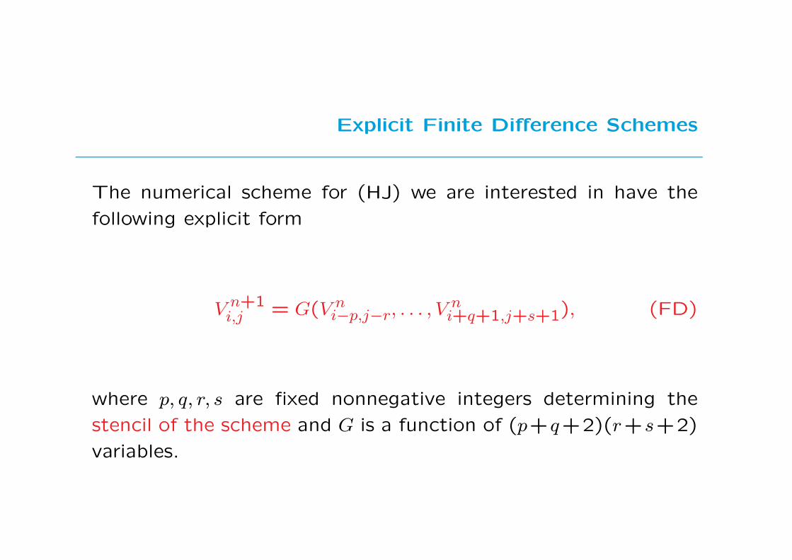
The numerical scheme for (HJ) we are interested in have the

following explicit form

V n+1i,j = G(V n

i−p,j−r, . . . , Vni+q+1,j+s+1), (FD)

where p, q, r, s are fixed nonnegative integers determining the

stencil of the scheme and G is a function of (p+q+2)(r+s+2)

variables.

Scheme in differenced form

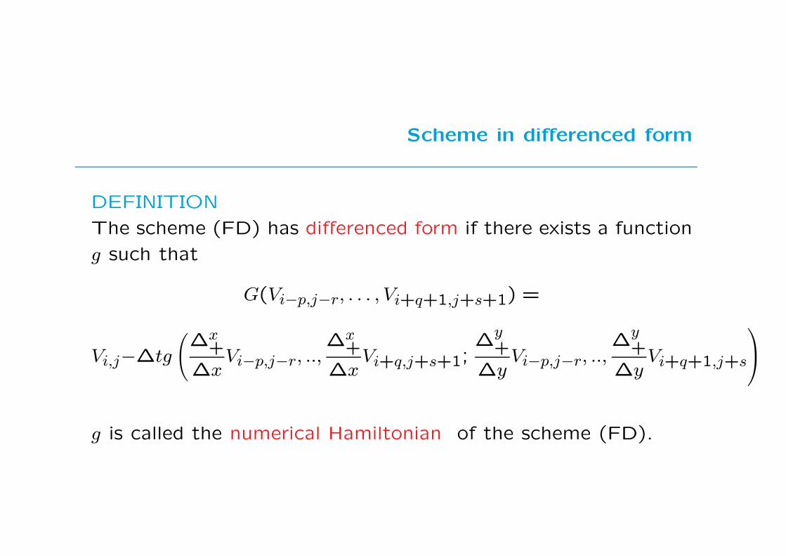
DEFINITION

The scheme (FD) has differenced form if there exists a function

g such that

G(Vi−p,j−r, . . . , Vi+q+1,j+s+1) =

Vi,j−∆tg

(

∆x+

∆xVi−p,j−r, ..,

∆x+

∆xVi+q,j+s+1;

∆y+

∆yVi−p,j−r, ..,

∆y+

∆yVi+q+1,j+s

g is called the numerical Hamiltonian of the scheme (FD).

Consistency

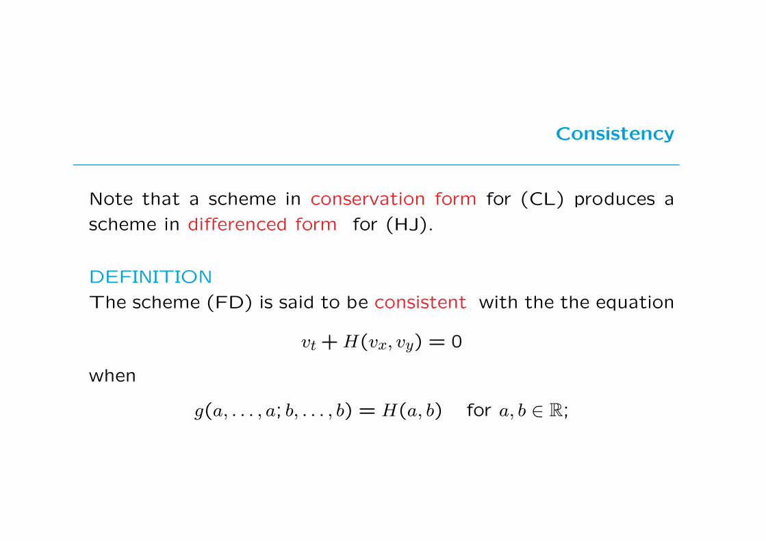
Note that a scheme in conservation form for (CL) produces a

scheme in differenced form for (HJ).

DEFINITION

The scheme (FD) is said to be consistent with the the equation

vt + H(vx, vy) = 0

when

g(a, . . . , a; b, . . . , b) = H(a, b) for a, b ∈ R;

Monotone FD Schemes

DEFINITION

The scheme (FD) is said to be monotone on [−R, R] if

G(Vi−p,j−r, . . . , Vi+q+1,j+s+1)

is a nondecreasing function of each argument as long as

|∆x+Vl,m|/∆x, |∆

y+Vl′,m′|/∆y ≤ R

for i − p ≤ l ≤ i + q, j − r ≤ m ≤ j + s + 1, i − p ≤ l′ ≤

i + q + 1, j − r ≤ m′ ≤ j + s

Roughly speaking, R is an a priori bound on |vx|, |vy| for the

solution of (HJ).

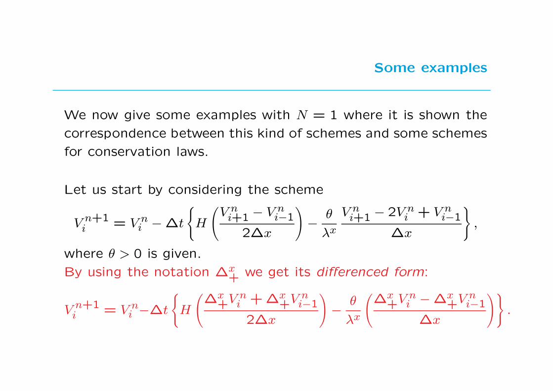
Some examples

We now give some examples with N = 1 where it is shown the

correspondence between this kind of schemes and some schemes

for conservation laws.

Let us start by considering the scheme

V n+1i = V n

i − ∆t

H

(

V ni+1 − V n

i−1

2∆x

)

−θ

λx

V ni+1 − 2V n

i + V ni−1

∆x

,

where θ > 0 is given.

By using the notation ∆x+ we get its differenced form:

V n+1i = V n

i −∆t

H

(

∆x+V n

i + ∆x+V n

i−1

2∆x

)

−θ

λx

(

∆x+V n

i − ∆x+V n

i−1

∆x

)

.

Lax-Friedrichs scheme

The numerical Hamiltonian is given by

g(α, β) = H

(

α + β

2

)

− (β − α)θ

λxfor α, β ∈ R. (LF)

As it is easy to check g(α, α) = H(α), hence the scheme is con-

sistent.

It is also monotone on [−R, R] if 1−2θ ≥ 0 (monotonicity in V ni ),

and θ − λx|H ′(α)|/2 ≥ 0 for |α| ≤ R (monotonicity in V ni+1, V n

i−1).

We obtain these two relations by first choosing 0 < θ < 1/2 and

then λx sufficiently small.

This scheme corresponds to the Lax-Friedrichs scheme for con-

servation laws.

Up-Wind scheme

The two “upwind” schemes

V n+1i = V n

i − ∆t H

(

V ni+1 − V n

i

∆x

)

, (UW–)

V n+1i = V n

i − ∆t H

(

V ni − V n

i−1

∆x

)

, (UW+)

have the requested monotonicity properties provided

H is nonincreasing for forward differences, i.e. (UW–)

H is nondecreasing for backward difference, i.e. (UW+)

and 1 ≥ λx|H ′(α)| for |α| ≤ R.

Convergence for monotone FD schemes

A general convergence result for monotone schemes in R has

been obtained by Crandall and Lions (1984).

Every FD scheme in differenced form for (EHJ) which is also

monotone and consistent will converge in the L∞ norm to the

viscosity solution

Unfortunately, monotone schemes have at most rate of conver-

gence 1 !

References

FINITE DIFFERENCES

M.G. Crandall, P.L. Lions, Two approximations of solutions of

Hamilton-Jacobi equations, Mathematics of Computation 43

(1984), 1-19.

J.A. Sethian, Level Set Method. Evolving interfaces in geom-

etry, fluid mechanics, computer vision, and materials science,

Cambridge Monographs on Applied and Computational Mathe-

matics, vol. 3, Cambridge University Press, Cambridge, 1996.

S. Osher, R.P. Fedkiw, Level Set Methods and Dynamic Implicit

Surfaces, Springer–Verlag, New York, 2003.

Semi-Lagrangian schemes

These schemes are based on a different idea which is to discretize

directly the ”directional derivative” which is hidden behind the

nonlinearity of the hamiltonian H(Du).

The goal is to mimic the method of characteristics by construct-

ing the solution at each grid point integrating back along the

characteristics passing through it and reconstructing the value

at the foot of the characteristic line by interpolation.

Semi-Lagrangian schemes

Let us start, writing the equation

ut + c(x)|Du(x)| = 0 (LS − HJ)

as

ut + maxa∈B(0,1)

[−c(x)a · Du(x)] = 0

Naturally, this is equivalent to our equation since plugging

a∗ =Du(x)

|Du(x)|

we get back to the first equation.

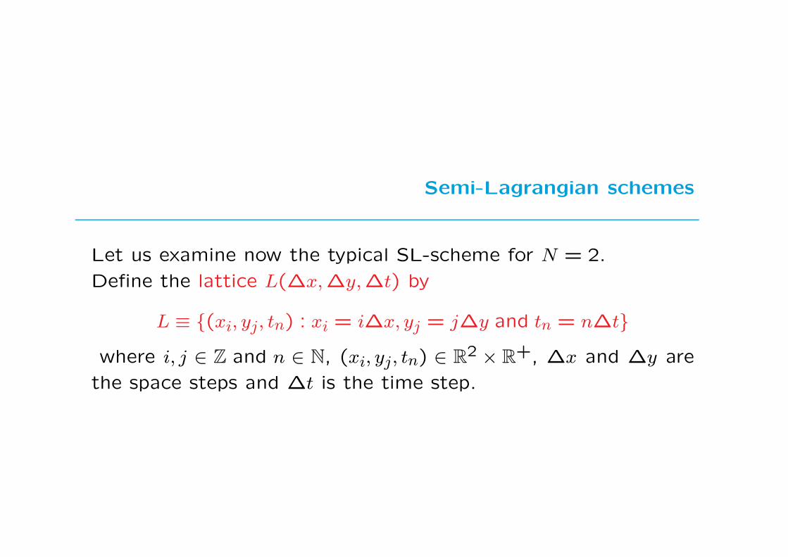
Semi-Lagrangian schemes

Let us examine now the typical SL-scheme for N = 2.

Define the lattice L(∆x,∆y,∆t) by

L ≡ (xi, yj, tn) : xi = i∆x, yj = j∆y and tn = n∆t

where i, j ∈ Z and n ∈ N, (xi, yj, tn) ∈ R2 × R+, ∆x and ∆y are

the space steps and ∆t is the time step.

Approximate Directional Derivatives

In order to obtain the SL-scheme let us consider the following

approximation for δ > 0

−a · Dv(xi, yj, tn) =v(xi − a1δ, yj − a2δ, tn) − v(xi, yj, tn)

δ+ O(δ)

We will use the standard notation

V nij ≈ v(xi, yj, tn), i, j ∈ Z and n ∈ N.

Since the the point (xi − a1δ, yj − a2δ) will not be nodes of the

lattice L we need to extend the solution everywhere in space by

interpolation V n : R2 → R.

This extension will allow to compute V n at any triple (x, y, tn).

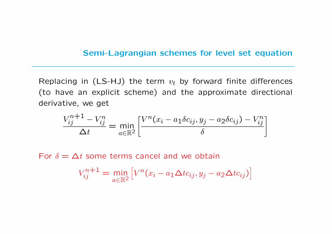
Semi-Lagrangian schemes for level set equation

Replacing in (LS-HJ) the term vt by forward finite differences

(to have an explicit scheme) and the approximate directional

derivative, we get

V n+1ij − V n

ij

∆t= min

a∈R2

[

V n(xi − a1δcij, yj − a2δcij) − V nij

δ

]

For δ = ∆t some terms cancel and we obtain

V n+1ij = min

a∈R2

[

V n(xi − a1∆tcij, yj − a2∆tcij)]

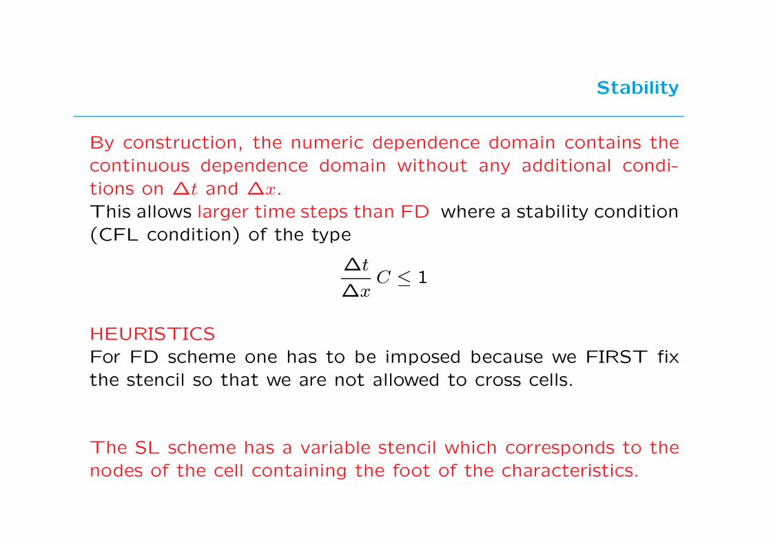
Stability

By construction, the numeric dependence domain contains the

continuous dependence domain without any additional condi-

tions on ∆t and ∆x.

This allows larger time steps than FD where a stability condition

(CFL condition) of the type

∆t

∆xC ≤ 1

HEURISTICS

For FD scheme one has to be imposed because we FIRST fix

the stencil so that we are not allowed to cross cells.

The SL scheme has a variable stencil which corresponds to the

nodes of the cell containing the foot of the characteristics.

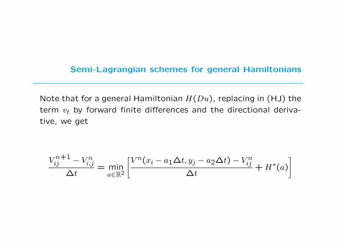
Semi-Lagrangian schemes for general Hamiltonians

Note that for a general Hamiltonian H(Du), replacing in (HJ) the

term vt by forward finite differences and the directional deriva-

tive, we get

V n+1ij − V n

i,j

∆t= min

a∈R2

[

V n(xi − a1∆t, yj − a2∆t) − V nij

∆t+ H∗(a)

]

Semi-Lagrangian schemes for general Hamiltonians

Finally, we can write the time explicit scheme

V n+1i,j = min

a∈R2

[

V n(xi − a1∆t, yj − a2∆t) + ∆tH∗(a)]

(SL)

Note that the SL-schemes has the same structure of the Hopf-

Lax representation formula of the exact solution written for v0 =

V n and t = ∆t.

Semi-Lagrangian schemes

In fact, taking the Hopf formula

v(x, t) = infy∈Rn

[

v0(y) + tH∗(

x − y

t

)]

and taking

a =x − y

tand t = ∆t

we immediately get

V n+1i,j = min

a∈R2

[

V n(xi − a1∆t, yj − a2∆t) + ∆tH∗(a)]

(SL)

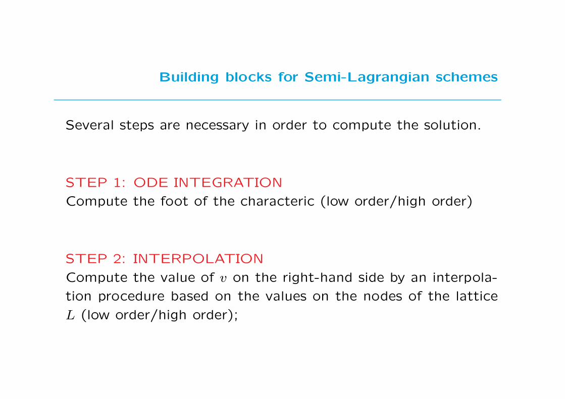
Building blocks for Semi-Lagrangian schemes

Several steps are necessary in order to compute the solution.

STEP 1: ODE INTEGRATION

Compute the foot of the characteric (low order/high order)

STEP 2: INTERPOLATION

Compute the value of v on the right-hand side by an interpola-

tion procedure based on the values on the nodes of the lattice

L (low order/high order);

Building blocks for Semi-Lagrangian schemes

STEP 3: LEGENDRE TRASFORM

Then, one has to determine H∗(a) ;

STEP 4: OPTIMIZATION

compute the minimum for a ∈ R2.

Note that the first two steps can be improved using high-order

methods.

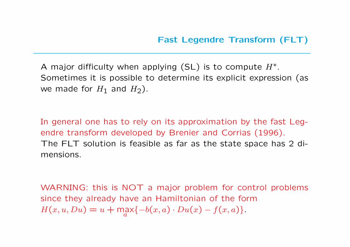
Fast Legendre Transform (FLT)

A major difficulty when applying (SL) is to compute H∗.

Sometimes it is possible to determine its explicit expression (as

we made for H1 and H2).

In general one has to rely on its approximation by the fast Leg-

endre transform developed by Brenier and Corrias (1996).

The FLT solution is feasible as far as the state space has 2 di-

mensions.

WARNING: this is NOT a major problem for control problems

since they already have an Hamiltonian of the form

H(x, u, Du) = u + maxa

−b(x, a) · Du(x) − f(x, a).

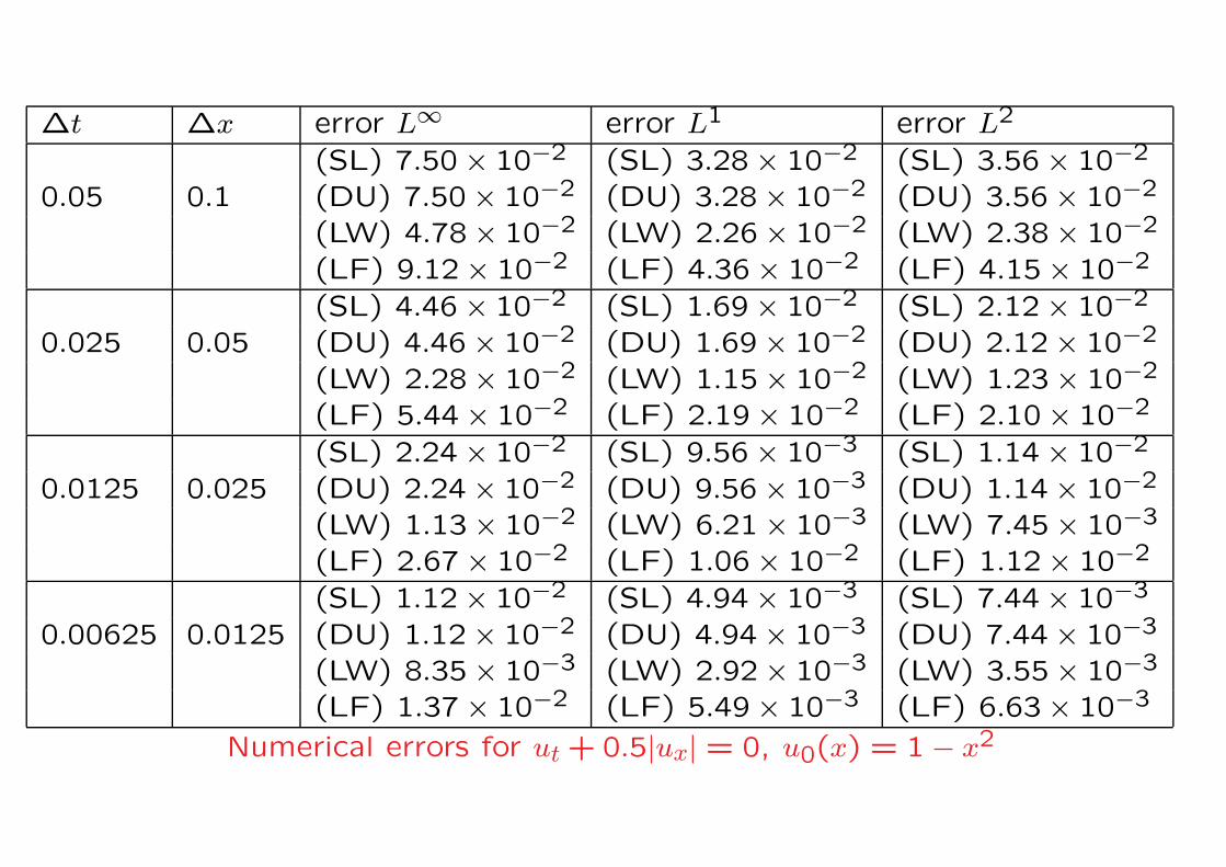
∆t ∆x error L∞ error L1 error L2

(SL) 7.50 × 10−2 (SL) 3.28 × 10−2 (SL) 3.56 × 10−2

0.05 0.1 (DU) 7.50 × 10−2 (DU) 3.28 × 10−2 (DU) 3.56 × 10−2

(LW) 4.78 × 10−2 (LW) 2.26 × 10−2 (LW) 2.38 × 10−2

(LF) 9.12 × 10−2 (LF) 4.36 × 10−2 (LF) 4.15 × 10−2

(SL) 4.46 × 10−2 (SL) 1.69 × 10−2 (SL) 2.12 × 10−2

0.025 0.05 (DU) 4.46 × 10−2 (DU) 1.69 × 10−2 (DU) 2.12 × 10−2

(LW) 2.28 × 10−2 (LW) 1.15 × 10−2 (LW) 1.23 × 10−2

(LF) 5.44 × 10−2 (LF) 2.19 × 10−2 (LF) 2.10 × 10−2

(SL) 2.24 × 10−2 (SL) 9.56 × 10−3 (SL) 1.14 × 10−2

0.0125 0.025 (DU) 2.24 × 10−2 (DU) 9.56 × 10−3 (DU) 1.14 × 10−2

(LW) 1.13 × 10−2 (LW) 6.21 × 10−3 (LW) 7.45 × 10−3

(LF) 2.67 × 10−2 (LF) 1.06 × 10−2 (LF) 1.12 × 10−2

(SL) 1.12 × 10−2 (SL) 4.94 × 10−3 (SL) 7.44 × 10−3

0.00625 0.0125 (DU) 1.12 × 10−2 (DU) 4.94 × 10−3 (DU) 7.44 × 10−3

(LW) 8.35 × 10−3 (LW) 2.92 × 10−3 (LW) 3.55 × 10−3

(LF) 1.37 × 10−2 (LF) 5.49 × 10−3 (LF) 6.63 × 10−3

Numerical errors for ut + 0.5|ux| = 0, u0(x) = 1 − x2

Convergence for SL schemes

Convergence for first order SL schemes for stationary and evo-

lutive HJ equations have been proved by F. (1987,...), F.-Giorgi

(1998).

A convergence result for high-order schemes in R has been

proved by Ferretti (2004) for the scheme

V nj = min

a∈RI[V n−1](xj − a∆t) + ∆tH∗(a)]

where I[·] is a generic interpolation operator on the grid.

Convergence for SL schemes

THEOREM

Assume that

(A1) H ′′ ≥ mH > 0

(A2)∆x = O(∆t2)

|I[v](x) − I1[v](x)| ≤ C max |Vj−1 − 2Vj + Vj+1| for C < 1

where I1 is linear interpolation operator.

Then, the scheme converges in L∞(Ω).

The HJPACK Library

HJPACK is a public domain library for Hamilton-Jacobi equa-

tions. It includes

• finite difference schemes and semi-Lagrangian schemes in R

and R2

• applications to control problems and front propagation

• fast-marching schemes

• a graphical interface and a user’s guide

You can get it at www.caspur.it/hjpack.

Basic references

SEMI-LAGRANGIAN SCHEMES

M. Falcone, T. Giorgi, An approximation scheme for evolutive

Hamilton–Jacobi equations, in W.M. McEneaney, G. Yin, Q.

Zhang (eds), ”Stochastic analysis, Control, optimization and

applications: a volume in honor of W.H. Fleming”, Birkhauser,

1998.

M. Falcone, R. Ferretti, Semi-Lagrangian schemes for Hamilton-

Jacobi equations discrete representation formulae and Godunov

methods, J. of Computational Physics, 175, (2002), 559-575.

Basic references

E. Carlini, R. Ferretti, G. Russo, A Weno large time-step for

Hamilton-Jacobi equation, SIAM J. Sci. Comput.

M. Falcone, R. Ferretti, Consistency of a large time-step scheme

for mean curvature motion, In F.Brezzi, A.Buffa, S.Corsaro and

A.Murli (eds), Numerical Analysis and Advanced Applications-

Proceedings on ENUMATH 2001, Ischia,(2001).

J. Strain, Semi-Lagrangian methods for level set equations, J.

Comput. Phys. 151 (1999), 498-533.

M. Falcone, R. Ferretti, Semi-Lagrangian approximation schemes

for linear and Hamilton-Jacobi equations, SIAM, to appear.

Basic References

FINITE ELEMENTS

Very few papers available.

A Discontinuous Galerkin approach has been developed by B.

Cockburn, C.W. Shu.

Recent contributions in the Ph.D. Thesis by Ch. Rasch (TU

Munich).

RATE OF CONVERGENCE

G. Barles, E.R. Jakobsen, On the convergence rate of approxi-

mation schemes for Hamilton-Jacobi-Bellman equations, Math.

Mod. Num. Anal. , 36 (2002), 33-54.

N. V. Krylov, On the rate of convergence of finite-difference ap-

proximations for Bellman’s equations with variable coefficients.

Probab. Theory Related Fields 117 (2000), no. 1, 1–16.