an inverse problem related to the hyperthermia …

AN INVERSE PROBLEM RELATED TO THE

HYPERTHERMIA TREATMENT OF CANCER

Bernard Lamien1, Helcio R. B. Orlande1,

Guillermo E. Eliçabe2, André J. Maurente3

1Federal University of Rio de Janeiro, PEM/COPPE, CP 68503, Rio de Janeiro,

RJ, 21941-972, Brazil, [email protected] 2Inst. Mat. Science and Technology (INTEMA), Univ. Mar del Plata (CONICET)

- Mar del Plata, Argentina 3Federal University of Rio Grande do Norte - UFRN, 59078-970, Natal, RN -

Brasil

1

Bernard Lamien, Helcio R. B. Orlande, Guillermo E. Eliçabe, André J. Maurente, State Estimation Problem In

Hyperthermia Treatment Of Tumors Loaded With Nanoparticles, Proceedings of the 15th International Heat Transfer

Conference, IHTC-15, August 10-15, 2014, Kyoto, Japan, IHTC15-8772

SUMMARY

• Motivation

• State estimation problems

• Particle filter – Algorithms and other

applications in Biomedical Engineering

• Test-case with simulated data: Model reduction

and Approximation Error Model

• Conclusions and Ongoing Work

Hyperthermia

• Temperature increase of body tissues, globally or locally,

possibly for therapeutic purposes.

• Dr. William Coley reported in 1891 the effect of fever on

tumors: Coley’s toxin, which was a cocktail of bacteria

(hyperthermia and immunotherapy).

• In thermoablation, heat is solely used for the destruction of

cancerous tissues. The term hyperthermia is used when heat

is applied to make tumors more vulnerable to other kinds of

treatment, such as radiotherapy and chemotherapy.

• Radio frequency ablation (RFA) is a current medical

procedure. Tissue is ablated using the heat generated from

high frequency alternating current (350–500 kHz).

MOTIVATION (See, for example, D. Chatterjee, S. Krishnan, Gold Nanoparticle –Mediated Hyperthermia in Cancer Therapy, Chapter

14 in Cancer Nanotechnology, editors S. Cho and S Krishnan, CRC Press, Boca Raton, 2013)

Hyperthermia

• Thermoablation causes direct cell necrosis (T > 50 oC).

• Hypertermia (41oC - 45oC) induces apoptosis (cell death

mechanism).

• Can be classified based on the target (Whole-body, Regional,

Local) or on the form (External, Interstitial, Intracavitary).

• In the Near Infrared (NIR) range (700 nm – 1400 nm)

hemoglobin and water absorption is minimum. Similar

behavior for Radio Frequency (RF) (3 kHz – 300 GHz).

• Heating time is also important: thermal dose

• Destruction of healthy cells and regrowth of tumor is a

problem.

MOTIVATION (See, for example, D. Chatterjee, S. Krishnan, Gold Nanoparticle –Mediated Hyperthermia in Cancer Therapy, Chapter

14 in Cancer Nanotechnology, editors S. Cho and S Krishnan, CRC Press, Boca Raton, 2013)

MOTIVATION

• Metallic nanoparticles exhibit Surface

Plasmon Resonance, which increases

absorption and scattering of light:

heating is enhanced.

• Plasmon is a quantum of the free

electrons ocillation.

• Nanoparticles can be made resonant

to particles at specific wavelengths.

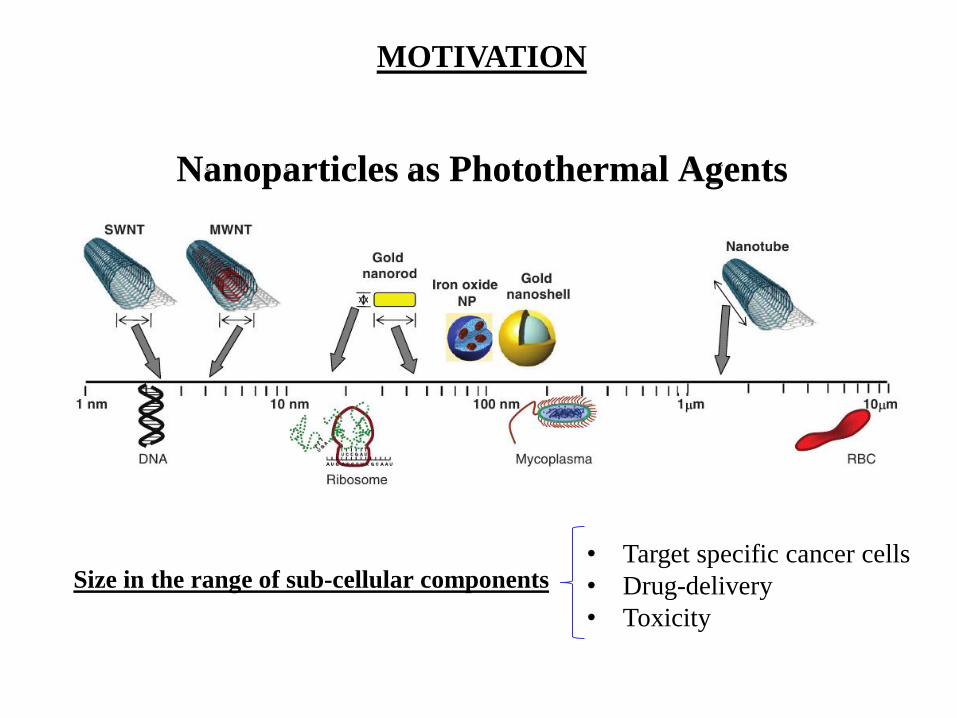
Nanoparticles as Photothermal Agents

Size in the range of sub-cellular components

MOTIVATION

• Target specific cancer cells

• Drug-delivery

• Toxicity

Inverse Problems in Hyperthermia

Dependence of the temperature distribution on laser parameters and tissue

properties, particularly blood perfusion coefficient. Tissue properties are

dependent of the physiological state and exhibit large variability from

individual to individual: Difficulty to predict a thermal dose

Hyperthermia treatment modalities requires generally treatment planning

even a predictive control of the temperature distribution in order to

minimize damage to healthy cells.

MRTI - Magnetic Ressonance Temperature Imaging can be used for

monitoring the delivery of thermal energy in tissues in real time (see R. Satfford,

J. Hazle, Magnetic Resonance Temperature imaging for Gold Nanoparticle-Mediated Thermal Therapy,

Chapter 15 in in Cancer Nanotechnology, editors S. Cho and S Krishnan, CRC Press, Boca Raton, 2013)

Uncertain models and uncertain measurements: Bayesian filters for the

solution of State Estimation problems

Particle filters: Computationally demanding, but Reduced Models can be

used together with the Approximation Error Model

MOTIVATION

STATE ESTIMATION PROBLEM

State Evolution Model:

Observation Model: ( , )k k k kz h x n

xnRx

Subscript k = 1, 2, …, denotes an instant tk in a

dynamic problem

= state variables to be estimated

vnRv

znRz

nnRn

= state noise

= measurements

= measurement noise

xk = fk (xk-1, uk-1, vk-1)

u R np = input variable


Definition: The state estimation problem aims at

obtaining information about xk based on the state

evolution model and on the measurements given by

the observation model.

The evolution-observation model is based on the following assumptions :

(i) The sequence kx for k = 1, 2, …, is a Markovian process, that is,

0 1 1 1( , , , ) ( )k k k k x x x x x x

(ii) The sequence kz for k = 1, 2, …, is a Markovian process with respect to

the history of kx

, that is,

0 1( , , , ) ( )k k k k z x x x z x

(iii) The sequence kx

depends on the past observations only through its own

history, that is,

1 1: 1 1( , ) ( )k k k k k x x z x x



xk = fk (xk-1, uk-1, vk-1)




xk = fk (xk-1, uk-1, vk-1)

1. The prediction problem, concerned with the determination of 1: 1( )k k x z ;

2. The filtering problem, concerned with the determination of 1:( )k k x z ;

3. The fixed-lag smoothing problem, concerned the determination of 1:( )k k p x z ,

where 1p

is the fixed lag;

4. The whole-domain smoothing problem, concerned with the determination of

1:( )k K x z , where 1: { , 1, , }K i i K z z is the complete sequence of

measurements.

Different problems can be considered:


(x0)

Prediction

(x1)

Update

(x1 |x0)

(z1 |x1)

(x1| z1)

Prediction

(x2 | z1)

Update

(x2 |x1)

(z2 |x2)

(x2| z1:2)

(x0)

Prediction

(x1)

Update

(x1 |x0)

(z1 |x1)

(x1| z1)

Prediction

(x2 | z1)

Update

(x2 |x1)

(z2 |x2)

(x2| z1:2)

FILTERING PROBLEM

By assuming that

is available, the posterior probability

density is then obtained

with Bayesian filters in two steps:

prediction and update

0 0 0( ) ( ) x z x

1:( )k k x z

THE KALMAN FILTER

• Evolution and observation models are linear.

• Noises in such models are additive and Gaussian, with

known means and covariances.

• Optimal solution if these hypotheses hold.

k k k k z H x n


Observation Model:

• F and H are known matrices for the linear evolutions of the state x and of the

observation z, respectively.

• G is matrix that determines how the control u affects the state x.

• Vector s is assumed to be a known input .

• Noises v and n have zero means and covariance matrices Q and R, respectively.

x𝑘− = F𝑘x𝑘−1 +G𝑘u𝑘−1 + s𝑘−1+v𝑘−1

THE PARTICLE FILTER

• Monte-Carlo techniques are the most general and robust for

non-linear and/or non-Gaussian distributions.

• The key idea is to represent the required posterior density

function by a set of random samples (particles) with associated

weights, and to compute the estimates based on these samples

and weights.

• Introduced in the 50’s, but not much used until recently

because of limited computational resources.

• Particles degenerated very fast in early implementations, i.e.,

most of the particles would have negligible weight. The

resampling step has a fundamental role in the advancement of

the particle filter.

Sampling Importance Resampling (SIR) Algorithm (Ristic, B., Arulampalam, S., Gordon, N., 2004, Beyond the Kalman Filter, Artech House, Boston)

Sampling Importance Resampling (SIR) Algorithm (Ristic, B., Arulampalam, S., Gordon, N., 2004, Beyond the Kalman Filter, Artech House, Boston)

Step 1

For 1, ,i N draw new particles xi

k from the prior

density 1x xi

k k and then use the likelihood density

to calculate the correspondent weights z xi i

k k kw .

Step 2

Calculate the total weight 1

Ni

w k

i

T w

and then normalize

the particle weights, that is, for 1, ,i N let 1i i

k w kw T w

Step 3

Resample the particles as follows :

Construct the cumulative sum of weights (CSW) by

computing 1

i

i i kc c w for 1, ,i N , with 0 0c .

Let 1i and draw a starting point 1u from the uniform

distribution 10,U N

For 1, ,j N

Move along the CSW by making 1

1 1ju u N j

While j iu c make 1i i .

Assign sample j i

k kx x

Assign sample 1j

kw N

• Weights are easily evaluated and

importance density easily

sampled.

• Sampling of the importance

density is independent of the

measurements at that time. The

filter can be sensitive to outliers.

• Resampling is applied every

iteration, which can result in fast

loss of diversity of the particles.

Auxiliary Sampling Importance Resampling (ASIR) Algorithm (Ristic, B., Arulampalam, S., Gordon, N., 2004, Beyond the Kalman Filter, Artech House, Boston)

Step 1

For i=1,...,N draw new particles xki from the prior density

(xk|xik-1) and then calculate some characterization of xk,

given xik-1, as for example the mean i

k=E[xk|xik-1]. Then

use the likelihood density to calculate the correspondent

weights wik=(zk|

ik)w

ik-1

Step 2

Calculate the total weight t=i wik and then normalize the

particle weights, that is, for i=1,...,N let wik = t-1 wi

k

Step 3

Resample the particles as follows :

Construct the cumulative sum of weights (CSW) by

computing ci=ci-1+wik for i=1,...,N, with c0=0

Let i=1and draw a starting point u1 from the uniform

distribution U[0,N-1]

For j=1,...,N

Move along the CSW by making uj=u1+N-1(j-1)

While uj>ci make i=i+1

Assign sample xjk=xi

k

Assign sample wjk=N-1

Assign parent ij=i

Step 4

For j=1,...,N draw particles xkj from the prior density

(xk|xij

k-1), using the parent ij, and then use the likelihood density to calculate the correspondent weights

wjk=(zk|x

jk) / (zk|

ijk)

Step 5

Calculate the total weight t=j wjk and then normalize the

particle weights, that is, for j=1,...,N let wjk = t-1 wj

k

• The advantage of ASIR over SIR is that

it naturally generates points from the

sample at k-1, which, conditioned on the

current measurement, are most likely to

be close to the true state.

• The resampling is based on some point

estimate ik that characterize (xk|x

ik-1),

which can be the mean ik=E[(xk|x

ik-1)]

or simply a sample of (xk|xik-1). If the

state evolution model noise is small,

(xk|xik-1) is generally well characterized

by ik, so that the weights wi

k are more

even and the ASIR algorithm is less

sensitive to outliers than the SIR

algorithm. On the other hand, if the state

evolution model noise is large, the single

point estimate ik in the state space may

not characterize well (xk|xik-1) and the

ASIR algorithm may not be as effective

as the SIR algorithm.

Application: Hodgkin-Huxley’s model Hodgkin, A.L., Huxley, A.F. "A Quantitative Description of Membrane Current and It's Application to Conduction and

Excitation in Nerve", Journal of Physiology, vol. 117, pp. 500-544, Mar. 1952.

• Action potential in excitable cells

• Sodium, Potassium and other ions accross the cell membrane

3 4máx máxmm Na m Na k m k L m L

dVI C G m h V V G n V V G V V

dt

1m m

dmm m

dt

(3.12)

1h h

dhh h

dt

(3.13)

1n n

dnn n

dt

(3.14) Diego C. Estumano, Helcio R. B. Orlande, Marcelo J. Colaço, George S. Dulikravich, State Estimation Problem For

Hodgkin-huxley´s Model: A Comparison Of Particle Filter Algorithms, 4th Inverse Problems, Design and Optimization

Symposium (IPDO-2013) Albi, France, June 26-28, 2013

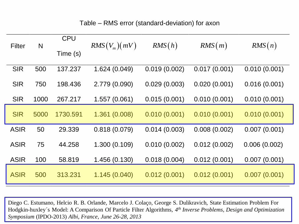
Table – RMS error (standard-deviation) for axon

Filter N CPU

Time (s) mRMS V mV RMS h RMS m RMS n

SIR 500 137.237 1.624 (0.049) 0.019 (0.002) 0.017 (0.001) 0.010 (0.001)

SIR 750 198.436 2.779 (0.090) 0.029 (0.003) 0.020 (0.001) 0.016 (0.001)

SIR 1000 267.217 1.557 (0.061) 0.015 (0.001) 0.010 (0.001) 0.010 (0.001)

SIR 5000 1730.591 1.361 (0.008) 0.010 (0.001) 0.010 (0.001) 0.010 (0.001)

ASIR 50 29.339 0.818 (0.079) 0.014 (0.003) 0.008 (0.002) 0.007 (0.001)

ASIR 75 44.258 1.300 (0.109) 0.010 (0.002) 0.012 (0.002) 0.006 (0.002)

ASIR 100 58.819 1.456 (0.130) 0.018 (0.004) 0.012 (0.001) 0.007 (0.001)

ASIR 500 313.231 1.145 (0.040) 0.012 (0.001) 0.012 (0.001) 0.007 (0.001)

Diego C. Estumano, Helcio R. B. Orlande, Marcelo J. Colaço, George S. Dulikravich, State Estimation Problem For



Axon

0 10 20 30 40 50 60-40

-20

0

20

40

60

80

100

120

time (ms)

Vm

(m

V)

Exact

Measurement

Estimated

99% Conf.Int




Axon

0 10 20 30 40 50 600

0.1

0.2

0.3

0.4

0.5

0.6

0.7

0.8

0.9

time (ms)

Innactivation h

Exact

Estimated

99% Conf.Int




Purkinje Fiber

100 200 300 400 500 600 700 800 900 1000

-80

-60

-40

-20

0

20

time (ms)

Vm

(m

V)

Exact

Measurement

Estimated

99% Conf.Int




Purkinje Fiber

0 100 200 300 400 500 600 700 800 900 1000-0.2

0

0.2

0.4

0.6

0.8

1

1.2

time (ms)

Innactivation h

Exact

Measurement

Estimated

99% Conf.Int




Simultaneous Estimation of State Variables and Model Parameters (J. Liu and M. West, Combined Parameter and State Estimation in Simulation-Based Filtering, Chapter 10 in

Sequential Monte Carlo Methods in Practice, Springer, ed. Doucet, A., Freitas, N. Gordon, N., 2001.)

• Evolution and observation models contain several constant

parameters, here denoted as the vector q.

• The above description of the particle filter method was based on a

deterministic vector q.

• However, in general such parameters are not deterministic or

might not be deterministically known.

• Therefore, the samples need to be extended to: { , : 0, , }i i

k k i Nx θ

1: 1: 1 1: 1( , ) ( , ) ( , ) ( )k k k k k k k x θ z z x θ x θ z θ z

2

1: 1 1 1 1

1

( ) ( , )N

i i

k k k k

i

w N h

θ z θ m V

APPLICATION: TUMOR SIZE EVOLUTION

This model involves as state variables the numbers of tumor (N1),

normal (N2) and angiogenic cells (L1), as well as the mass of the

chemotherapy drug in body (Q). It deals with the use of one single

chemotherapy cycle-unspecific agent, in a neoadjuvant treatment.

11 1 1 1 1 1 1 2 1 1 1

( )( , ) ( , , ) ( , )

d N tr N f N L g N N L h N Q

dt (1.a)

22 2 2 2 2 1 2 1 2 2

( )( ) ( , , ) ( , )

d N tr N f N g N N L h N Q

dt (1.b)

11 1 1 1 1 3 1

( )( ) ( , ) ( , ) ( , )

d L tm L n N L p N L h L Q

dt (1.c)

1 2

( )( ) ( , , )

dQ tq t u N N Q

dt (1.d)

Model developed by Diego Rodrigues, Paulo Mancera and Suani de Pinho

ri is the rate of cell population growth, fi(.) is the growth inhibition due to the

competition among cells of the same type for nutrients, etc, and gi(.) is the growth

inhibition due to the competition among cells of different types for nutrients, etc.

The functions hi(.), for i = 1, 2 and 3, model the interactions of the cell populations

with the chemotherapy drug. Hence, note that h3(.) models the antiangiogenic

effects of the chemotherapy agent. The tumor capacity to induce vascularization is

represented by n(.), while the body capacity to inhibit vascularization is modeled

by p(.). The function m(.) models the proliferation of endothelial cells and their

migration towards the tumor internal region. The infusion of the chemotherapy

agent is given by q(t), while u(.) is the model for the drug consumption and

excretion. 1

1 1 1 1 1 1 1 2 1 1 1

( )( , ) ( , , ) ( , )

d N tr N f N L g N N L h N Q

dt (1.a)

22 2 2 2 2 1 2 1 2 2

( )( ) ( , , ) ( , )

d N tr N f N g N N L h N Q

dt (1.b)

11 1 1 1 1 3 1

( )( ) ( , ) ( , ) ( , )

d L tm L n N L p N L h L Q

dt (1.c)

1 2

( )( ) ( , , )

dQ tq t u N N Q

dt (1.d)

APPLICATION: TUMOR SIZE EVOLUTION

1 1 1 2 11 1

1 1

( )1

d N t N N N Qr N

dt k L k L a Q

(7.a)

2 2 2 1 22 2

2 2

( )1

d N t N N N Qr N

dt k k b Q

(7.b)

1 11 1 1 1

( )d L t L QL N L N

dt c Q

(7.c)

( )( )

dQ tq t Q

dt (7.d)

• The simulated measured data was generated for a case involving a standard

chemotherapy protocol for the treatment of pancreatic cancer based on

GEMZAR®.

• The protocol consists of one intravenous administration per week for three

consecutive weeks, followed by one week of rest.

• The simulated measurements of the numbers of tumor and normal cells were

supposedly available periodically, every seven days after beginning of the

treatment.

-20 0 20 40 60 80 100 120 1400.5

1

1.5

2

2.5

3

3.5x 10

9

Time, days

Num

ber

of

tum

or

cells

Exact

Measured

Estimated

99% Upper Bound

99% Lower Bound

Measurements used

(a)

-20 0 20 40 60 80 100 120 1403

4

5

6

7

8

9

10

11

12

13x 10

12

Time, days

Num

ber

of

norm

al cells

Exact

Measured

Estimated

99% Upper Bound

99% Lower Bound

Measurements used

(b)

0 20 40 60 80 100 1200

0.5

1

1.5

2

2.5

3

3.5x 10

11

Time, days

Num

ber

of

angio

genic

cells

Exact

Estimated

99% Bounds

(c)

0 20 40 60 80 100 120-1

0

1

2

3

4

5

6x 10

-4

Time, days

Mass o

f dru

g in t

he b

lood,

mg

Exact

Estimated

99% Bounds

(d)

0 20 40 60 80 100 1200.008

0.0085

0.009

0.0095

0.01

0.0105

0.011

0.0115

0.012

Time, days

r 1,

day

-1

Exact

Estimated

99% Bounds

(a)

0 20 40 60 80 100 1200.85

0.9

0.95

1

1.05

1.1

1.15

1.2

1.25x 10

-3

Time, days

r 2,

day

-1

Exact

Estimated

99% Bounds

(b)

0 20 40 60 80 100 1200.85

0.9

0.95

1

1.05

1.1

1.15

1.2x 10

-3

Time, days

,

day

-1

Exact

Estimated

99% Bounds

(c)

0 20 40 60 80 100 12010.5

11

11.5

12

12.5

13

13.5

14

14.5

Time, days

,

day

-1

Exact

Estimated

99% Bounds

(d)

Hyperthermia Treatment of Cancer - Nanoparticles

Leonid A. Dombrovsky, Victoria Timchenko, Michael Jackson, Guan H. Yeoh, A combined transient thermal

model for laser hyperthermia of tumors with embedded gold nanoshells, International Journal of Heat and

Mass Transfer, Volume 54, Issues 25–26, December 2011, Pages 5459–5469

TEST-CASE

,

, ,, ,

0 , 0

p b p b b b met laser

T z t dT z tdz c z k z c z T T z t Q z Q z t

t dz dz

z d t

(1.a)

0, , 0 , 0T z t T z t (1.b)

0

,, , , 0

T z tk z hT z t hT z d t

z

(1.c)

0, , 0 , 0T z t T z d t (1.d)

with,

, ;laserQ z t z z t (1.e)

where, the subscript b refers to blood properties, b (s-1

) is the blood perfusion rate, Qmet (Wm-3

) is the heat generation resulting from metabolism, Qlaser (Wm

-3) is the heat source resulting from the laser absorption in

the tissues, (m-1

) is the absorption coefficient and (Wm-2) is the laser total fluence rate.

BIOHEAT TRANSFER EQUATION

TEST-CASE

a. COMPLETE MODEL FOR THE LASER FLUENCE RATE

Diffusion approximation in non-homogeneous medium on a fine mesh (Andre Maurente, Bernard Lamien, Helcio R. B. Orlande, Guillermo E. Eliçabe,

Analysis of the P1-approximation for the radiative heat transfer in skin tissues loaded

with nanoparticles, 22nd International Congress of Mechanical Engineering COBEM

2013, November 3-7, 2013, Ribeirão Preto, SP, Brazil)

b. REDUCED MODEL FOR THE FLUENCE RATE

Semi-infinite homogeneous medium on a coarse mesh (Welch, A.J., van Gemert M.J.C., Optical thermal response of laser irradiated tissue,

2nd Edition, Springer, 2011).

State Estimation problem with:

TEST-CASE

ESTIMATION WITH THE COMPLETE MODEL

(250 PARTICLES, LIU&WEST’S ALGORITHM)

TEST-CASE

0 0.5 1 1.5 2 2.5 3 3.5

37

37.5

38

38.5

39

39.5

40

40.5

41

41.5

42

z(mm)

T (o C

)

Estimadas

Exatas

99% Intervalo de Confiança, t=10 s

99% Intervalo de Confiança, t=25 s

t=10 s

t=25 s

Estimated

Exact

99% confidence interval, t=10s

99% confidence interval, t=25s

ESTIMATION WITH THE REDUCED MODEL

0 0.5 1 1.5 2 2.5 3 3.5

37

37.5

38

38.5

39

39.5

40

40.5

41

41.5

z(mm)

T (o

C)

Estimadas

Exatas

99% Intervalo de Confiança

t=5 s

Estimated with the reduced model

Exact

99% Confidence interval

TEST-CASE

Conventional Error Model

• State Evolution Model

• Observation Model

• Assuming the measurements errors Gaussian with zero mean and known

covariance matrix, the likelihood function is given as:

1 1, , , 1,...,k k k k k M x f x θ w

, , , 1,...,k k k k k M z g x θ v

11( | , ) exp [ , ] [ , ]

2

T

k k k k k k k k k

z x θ z g x θ W z g x θ

TEST-CASE

Approximation Error Model

• Let and be the reduced models associated to the more

accurate but computationally expensive models and

• Lets consider a linear operator, so that,

• We can write the state evolution-obsevation model as:

with,

with,

, ,r r r r

k k kf x θ w ,r r r

k kg x θ

, ,k k kf x θ w ,k kg x θ

xPr

k x kPx x

1, ,r r r r r r

k k k k k x f x θ w ω , , , ,r r r r r

k x k k k k k kP ω f x θ w f x θ w

,r r r r

k k k k k z g x θ υ v , ,r r r

k k k k x kP υ g x θ g x θ

TEST-CASE

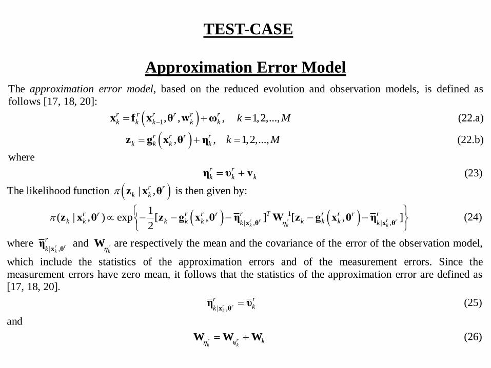
Approximation Error Model

The approximation error model, based on the reduced evolution and observation models, is defined as

follows [17, 18, 20]:

1, , , 1,2,...,r r r r r rk k k k k k M x f x θ w ω (22.a)

, , 1,2,...,r r r rk k k k k M z g x θ η (22.b)

where

r rk k k η υ v (23)

The likelihood function | ,r rk k z x θ is then given by:

1

| , | ,

1( | , ) exp [ , ] [ , ]

2r r r r rk k k

r r r r r r T r r r rk k k k k k k kk k

x θ x θ

z x θ z g x θ η W z g x θ η (24)

where | ,r r

k

r

k x θη and r

kW are respectively the mean and the covariance of the error of the observation model,

which include the statistics of the approximation errors and of the measurement errors. Since the

measurement errors have zero mean, it follows that the statistics of the approximation error are defined as [17, 18, 20].

| ,r r

k

r rkk

x θ

η υ (25)

and

r rk k

k

υW W W (26)

TEST-CASE

CONVERGENCE OF THE MODELING ERROR - Mean

0 0.5 1 1.5 2 2.5 3 3.5

-2

-1

0

1

2

3

z(mm)

e

rro (

oC

)

200 amostras

400 amostras

600 amostras

800 amostras

1000 amostras

1200 amostras

1400 amostras

1600 amostras

1800 amostras

2000 amostras

t=5 s

SAMPLES

TEST-CASE

CONVERGENCE OF THE MODELING ERROR

0 200 400 600 800 1000 1200 1400 1600 1800 20000.305

0.31

0.315

0.32

0.325

0.33

0.335

tot

Número de AmostrasNumber of Samples

Tra

ce o

f th

e C

ovariance M

atr

ix

t=5 s

TEST-CASE

ESTIMATED TEMPERATURE – PARTICLE FILTER

LIU&WEST’S ALGORITHM + AEM

TEST-CASE

0 0.5 1 1.5 2 2.5 3 3.5

37

38

39

40

41

42

z(mm)

T (

oC

)

Estimates

Exact

99% Confidence Interval, t=10 s

99% Confidence Interval, t=25 s

t=10 st=10 s

t=25 s

0 10 20 30 40 50 6036

37

38

39

40

41

42

43

44

t(s)

T (

oC

)

Exact

Estimates

Simulated Measurements

z = 0.36 mm



TEST-CASE

0 10 20 30 40 50 6037

37.5

38

38.5

39

39.5

40

40.5

41

41.5

t(s)

T (

oC

)

Exact

Estimates

Simulated Measurements

z = 1.49 mm



TEST-CASE

CONCLUSIONS

• Particle filter is the most general and robust technique for non-

linear models and/or non-Gaussian distributions.

• Even for large values of standard deviations in the evolution and

observation models, the estimated means are in excellent

agreement with the exact values of state variables and

model parameters.

• Although the state estimation problem was solved with a

reduced model over a coarse mesh and with a formulation

that neglects several physical aspects of the original

physical problem, the approximation error model was

capable of statistically taking into account the

discrepancies between the complete and reduced models,

thus resulting in accurate estimates of the transient

temperature fields.

ONGOING WORK

• 2D with axial symmetry with NIR Heating

• 3D with complex geometry (thyroid) with NIR Heating

• 3D with complex geometry (pancreas) with RF Heating

• Validation with experimental data obtained with phantoms

(Being developed in our Laboratory).

From left to right, phantoms made of: PVC-P, PVC-P and SiO2 nanoparticles

(3%wt) , PVC-P and thermal paste, PVC-P and TiO2 nanoparticles (0.7% wt)

Materials

Materials

Carbon Nanotubes – home-made

Diameter of 80 nm and length around 2 m

Concentration 0.1%wt

Single-Layer and Two-Layer phantoms

3.30 ± 0.03 mm

3.26 ± 0.06 mm

25.4 mm ±0.02

PVC-P

PVC-P with CNT

Experimental Setup

Laser diode was set to deliver a specified power on continuous wave mode through the collimator (mean wavelength of 829.1 nm).

An IR thermographic camera (FLIR, Thermacam SC660), placed at a distance of 40 cm above the phantom, measures the surface temperature

TC measurements at the non-heated surface

28.8

28.9

29

29.1

29.2

29.3

29.4

29.5

29.6

29.7

29.8

0 5 10 15 20 25 30 35 40 45 50

Tem

pera

ture

(ºC

)

Position (mm)

IR Irradiation - Start

900 mA

Li1

Li2

Li3

Li4

Li5

Temperature variations at the Carbon

Nanotube Phantom Surface – Two Layers

28.8

29

29.2

29.4

29.6

29.8

30

30.2

30.4

0 5 10 15 20 25 30 35 40 45

Tem

pera

ture

(ºC

)

Position (mm)

IR Irradiation - 20s

900 mA

Li1

Li2

Li3

Li4

Li5



28.5

29

29.5

30

30.5

31

31.5

0 5 10 15 20 25 30 35 40 45

Tem

pera

ture

(ºC

)

Position (mm)


900 mA

Li1

Li2

Li3

Li4

Li5



28.5

29

29.5

30

30.5

31

31.5

32

32.5

0 5 10 15 20 25 30 35 40 45

Tem

pera

ture

(ºC

)

Position (mm)


900 mA

Li1

Li2

Li3

Li4

Li5



Ackowledgements

The authors are thankful for the support provided by

CNPq, CAPES and FAPERJ, Brazilian agencies for the

fostering of science.

DEDICATION

57

HELCIO ORLANDE

11/12/1938 – 10/09/2012

an inverse problem related to the hyperthermia …

Documents