AN INVESTIGATION OF A LARGE

STEP-DOWN RATIO PARAMETRIC

SONAR AND ITS USE IN SUB-

BOTTOM PROFILING

Neil W. Fried

B.A.Sc. (Elec. Eng.), University of British Columbia, 1986

A THESIS SUBMITTED IN PARTIAL FULFILMENT OF THE

REQUIREMENTS FOR THE DEGREE OF

MASTER OF APPLIED SCIENCE (ENGINEERING SCIENCE)

/- in the school

of

Engineering Science

O Neil W. Fried 1992 Simon Fraser University

August 1992

All rights reserved. This thesis may not be reproduced in whole or in part, by photocopy or other means,

without the permission of the author.

Approval

NAME: Neil W. Fried

DEGREE: Master Applied Science (Engineering Science)

TITLE OF THESIS: An Investigation of a Large Step-Down Ratio Parametric Sonar and Its Use in Sub-Bottom Profiling

EXAMINING COMMITTEE:

Chairman: Dr. John Jones

6r. Pe'ter FOX

Supervisor

- - - Dr. ficquis Vaisey

Dr. Andrew Rawia Examiner

PARTIAL COPYRIGHT LICENSE

I hereby grant to Simon Fraser University the right to lend my thesis, project or

extended essay (the title of which is shown below) to users of the Simon Fraser University Library, and to make partial or single copies only for such users or in response to a request from the library of any other university, or other educational institution, on its own behalf or for one of its users. I further agree that permission for multiple copying of this work for scholarly purposes may be granted by me or the Dean of Graduate Studies. It is understood that copying or publication of this work for financial gain shall not be allowed without my written permission.

Title of Thesis/Project/Extended Essay

An Investigation of a Large Step-Down Ratio Parametric Sonar and Its Use - --

in Sub-bottom Profiling

Author: (signature)

August 11, 1992

iii

Abstract

A high resolution sub-bottom profiler is required which is small and light

weight for attaching to remotely operated vehicles (ROVs) used in mine

countermeasure operations. A large step-down ratio parametric sonar is investigated

in this thesis to determine if it provides a viable solution.

Computer modelling of the parametric array was done to better understand its

behaviour within the interaction region. A working prototype was developed and

used to verify the theoretical predictions. Results obtained illustrate the importance of

the primary wave beam characteristics in determining the secondary beamwidth, and

confirmed the high conversion losses for parametric sources with large frequency

step-down ratios. The results of a theoretical investigation of the water-sediment

interface are used along with the sonar equations to obtain performance limits for the

profiler in a side scan configuration. Experimental results are presented which show

normal incident penetration of a sediment bottom and confirm that the detection of a

buried pipe is possible.

Acknowledgements

I wish to thank Dr. John Bird and Dr. Peter Fox for their guidance and support

which made this project possible.

Appreciation is also extended to several past and present members of the

Underwater Research Laboratory. Special thanks to both Bill (Dr. "Physics")

McMullan and Harry Bohm for their assistance and encouragement. I would also like

to thank William Hue for his hardware and UNIX expertise, and (almost Dr.) Martie

Goulding for demonstrating that FORTRAN still lives on.

I express my gratitude to Simrad Mesotech System's Ltd. for their support of

this work through donations of equipment and materials, and use of facilities.

Finally, for my wife, Kris, I thank you for your support and patience.

Table of Contents

Approval . . . . . . . . . . . . . . . . . . . . . . . . . . . . . . . . . . . . . . . . . . . . . . . . . . . . . . . . . . ii

Abstract . . . . . . . . . . . . . . . . . . . . . . . . . . . . . . . . . . . . . . . . . . . . . . . . . . . . . . . . . iii

List of Figures . . . . . . . . . . . . . . . . . . . . . . . . . . . . . . . . . . . . . . . . . . . . . . . . . . . . vi

List of Tables . . . . . . . . . . . . . . . . . . . . . . . . . . . . . . . . . . . . . . . . . . . . . . . . . . . . viii

1 . Introduction . . . . . . . . . . . . . . . . . . . . . . . . . . . . . . . . . . . . . . . . . . . . . . . . . . . . 1 1.1. Background and Motivation for Research . . . . . . . . . . . . . . . . . . . . . . . 1 1.2. Research Objective and Methodology . . . . . . . . . . . . . . . . . . . . . . . . . . 6 1.3. Outline of Thesis . . . . . . . . . . . . . . . . . . . . . . . . . . . . . . . . . . . . . . . . . 7 References . . . . . . . . . . . . . . . . . . . . . . . . . . . . . . . . . . . . . . . . . . . . . . . . . . 9

2 . Nonlinear Acoustics . . . . . . . . . . . . . . . . . . . . . . . . . . . . . . . . . . . . . . . . . . . . . 10 2.1. Parametric Acoustic Arrays . . . . . . . . . . . . . . . . . . . . . . . . . . . . . . . . 10 2.2. Finite-Amplitude Distortion . . . . . . . . . . . . . . . . . . . . . . . . . . . . . . . . 21 References . . . . . . . . . . . . . . . . . . . . . . . . . . . . . . . . . . . . . . . . . . . . . . . . . 25

3 . Design of Parametric Sonar Systems . . . . . . . . . . . . . . . . . . . . . . . . . . . . . . . . . 27 3.1. Design Criteria . . . . . . . . . . . . . . . . . . . . . . . . . . . . . . . . . . . . . . . . . . 28 3.2. Prototype . . . . . . . . . . . . . . . . . . . . . . . . . . . . . . . . . . . . . . . . 33 References . . . . . . . . . . . . . . . . . . . . . . . . . . . . . . . . . . . . . . . . . . . . . . . . . 52

4 . Secondary Wave Characteristics . . . . . . . . . . . . . . . . . . . . . . . . . . . . . . . . . . . . 53 4.1. Circular Element Parametric Array Model . . . . . . . . . . . . . . . . . . . . . 53 4.2. Experimental Results . . . . . . . . . . . . . . . . . . . . . . . . . . . . . . . . . . . . . 57 4.3. Fan-Beam Design . . . . . . . . . . . . . . . . . . . . . . . . . . . . . . . . . . . . . . . . 69 References . . . . . . . . . . . . . . . . . . . . . . . . . . . . . . . . . . . . . . . . . . . . . . . . . 76

5 . Sub-Bottom Profiler Design . . . . . . . . . . . . . . . . . . . . . . . . . . . . . . . . . . . . . . . 77 5.1. Water-Sediment Interface . . . . . . . . . . . . . . . . . . . . . . . . . . . . . . . . . . 77 5.2. TheSonarEquations . . . . . . . . . . . . . . . . . . . . . . . . . . . . . . . . . . . . . . 85 5.3. Performance Evaluation of Prototype . . . . . . . . . . . . . . . . . . . . . . . . . 96 References . . . . . . . . . . . . . . . . . . . . . . . . . . . . . . . . . . . . . . . . . . . . . . . . 110

6 . Conclusions . . . . . . . . . . . . . . . . . . . . . . . . . . . . . . . . . . . . . . . . . . . . . . . . . 112

List of Figures

Figure 1 . 1 Comparison of Area Coverage for Beamwidths of 25 Degrees and 2Degrees . . . . . . . . . . . . . . . . . . . . . . . . . . . . . . . . . . . . . . . . . . . . . . . . . . . .

Figure 1.2 Illustration of Increased Area Coverage and Resolution with Side Scan Configuration . . . . . . . . . . . . . . . . . . . . . . . . . . . . . . . . . . . . . . . . . .

Figure 2.1 The Processes Involved in the Generation of the Diference Frequency Wave . . . . . . . . . . . . . . . . . . . . . . . . . . . . . . . . . . . . . . . . . . . . . .

. . . . . . . . . . Figure 2.2 The Stages of Nonlinear Wave Distortion and Shock Formation Figure 3.1 Block Diagram of an Echo Sounder . . . . . . . . . . . . . . . . . . . . . . . . . . . . . . Figure 3.2 Block Diagram of Prototype Used to Evaluate a

Parametric Sonar System . . . . . . . . . . . . . . . . . . . . . . . . . . . . . . . . . . . . . . . . Figure 3.3 cross-~ectionalhnd Top Views of Single Element Transducer . . . . . . . . . . . Figure 3.4 Equivalent Circuit for a Peizoelectric Transducer . . . . . . . . . . . . . . . . . . . . Figure 3.5 Circuit Diagram of Subsea Electronics Used in Inte$xing

to the 1 MHz Transducer . . . . . . . . . . . . . . . . . . . . . . . . . . . . . . . . . . . . . . . . Figure 3.6 Circuit Diagram for Subsea Electronics Used in Intofacing

to the Seperate Hydrophone . . . . . . . . . . . . . . . . . . . . . . . . . . . . . . . . . . . . . . Figure 3.7 Block Diagram of the 1 MHz SMSL Receiver Board . . . . . . . . . . . . . . . . . . Figure 3.8 Block Diagram of the 6.4 kHz SMSL Receiver Board . . . . . . . . . . . . . . . . . . Figure 3.9 Beam Pattern of 1 MHz Primary Wave . . . . . . . . . . . . . . . . . . . . . . . . . . . Figure 3.10 Beam Pattern of 0.9936 MHz Primary Wave . . . . . . . . . . . . . . . . . . . . . . Figure 4.1 Geometry for Circular Transducer Model . . . . . . . . . . . . . . . . . . . . . . . . . . Figure 4.2 Theoretical Source Level of Secondary Wave . . . . . . . . . . . . . . . . . . . . . . . . Figure 4.3 Theoretical Beam Patterns of Secondary Wave at 5 and 10 meters

(The Wider Beam is for a Range of 10 meters) . . . . . . . . . . . . . . . . . . . . . . . . . Figure 4.4 Theoretical Beamwidth of Secondary Wave . . . . . . . . . . . . . . . . . . . . . . . . . Figure 4.5 Received Pulse for Prima y Waves . . . . . . . . . . . . . . . . . . . . . . . . . . . . . . . Figure 4.6 Received Pulse for Secondmy Wave . . . . . . . . . . . . . . . . . . . . . . . . . . . . . . Figure 4.7 Theoretical and Experimental Secondary Wave Beam Patterns at

. . . . . . . . . . . . . . . . . . . . . . . . . . . . . . . . . . . . . . . . . . . . . . . . . . . lometers Figure 4.8 Theoretical and Experimental Secondary Wave Beam Pattern

at 10 meters with Primary Wave Beam Pattern . . . . . . . . . . . . . . . . . . . . . . . . Figure 4.9 Theoretical and Experimental Secondary Wave Source Levels

with Primary Wave Source h e 1 . . . . . . . . . . . . . . . . . . . . . . . . . . . . . . . . . . Figure 4.10 Theoretical and Experimental Seconda y Wave Reamwid ths . . . . . . . . . . . . Figure 4.1 1 Theoretical and Experimental Secondary Wave Source Levels

Obtained in Test Tank . . . . . . . . . . . . . . . . . . . . . . . . . . . . . . . . . . . . . . . . . . Figure 4.12 Geometry for Rectangular Transducer Model . . . . . . . . . . . . . . . . . . . . . . Figure 5.1 Geomety of the Water-Sediment Int4ace . . . . . . . . . . . . . . . . . . . . . . . . . Figure 5.2 Illustration of Sonar Equation Parameters . . . . . . . . . . . . . . . . . . . . . . . . . Figure 5.3 Sub-Bottom Profiler Design Spreadsheet for Parametric

Sonar (page 1) . . . . . . . . . . . . . . . . . . . . . . . . . . . . . . . . . . . . . . . . . . . . . . . Figure 5.4 Sub-Bottom Profiler Design Spreadsheet for Parametric

. . . . . . . . . . . . . . . . . . . . . . . . . . . . . . . . . . . . . . . . . . . . . . . Sonar (yage 2)

vii

Figure 5.5 Sub-Bottom Profder Design Spreadsheet for Parametric Sonm (page 3) . . . . . . . . . . . . . . . . . . . . . . . . . . . . . . . . . . . . . . . . . . . . . . . 95

Figure 5.6 SNRs for Electrical and Acoustical Noise. and TRR (OCV = .208.3 dB) . . . . . . . . . . . . . . . . . . . . . . . . . . . . . . . . . . . . . . . . 98

Figure 5.7 SNRs for Electrical and Acoustical Noise. and TRR (OCV = .183.5 dB) . . . . . . . . . . . . . . . . . . . . . . . . . . . . . . . . . . . . . . . . 99

Figure 5.8 Maximum True Range versus Target Depth (OCV = .183.5 dB) . . . . . . . . 100 Figure 5.9 Top View of Site Layout for Piling Tests . . . . . . . . . . . . . . . . . . . . . . . . . 103 Figure 5.10 Return Signal of Pilings . . . . . . . . . . . . . . . . . . . . . . . . . . . . . . . . . . . . 104 Figure 5.11 Expanded View of Piling Returns for 500 pec Pulse h g t h . . . . . . . . . . 104 Figure 5.12 Expanded View of Piling Returns for a 700 psec Pulse Leng . . . . . . . . . . 105 Figure 5.13 Site Layout for Sub-Bottom Tests . . . . . . . . . . . . . . . . . . . . . . . . . . . . . . 106 Figure 5.14 Bottom Return with a Target . . . . . . . . . . . . . . . . . . . . . . . . . . . . . . . . 107 Figure 5.15 Bottom Return without a Target . . . . . . . . . . . . . . . . . . . . . . . . . . . . . . 107

viii

List of Tables

Table 3.1 Primary Wave Input Powers m d Source Levels . . . . . . . . . . . . . . . . . . . . . . 48 Table 4.1 Secondary Wave Characteristics for Several Rectangular Transducer

Dimensions at 10 meters . . . . . . . . . . . . . . . . . . . . . . . . . . . . . . . . . . . . . . . . 73 Table 4.2 Secondary Wave Characteristics for Two Rectangular Transducer

Dimensions at 50 meters . . . . . . . . . . . . . . . . . . . . . . . . . . . . . . . . . . . . . . . . 74

1. Introduction

1.1. Background and Motivation for Research

1.1.1. Current Sub-Bottom Profilers

Sub-bottom profilers are imaging sonars which are pointed vertically at the

ocean floor and generally operate at frequencies below 10 kHz. The low frequency

acoustic signal penetrates the marine sediments which permits geotechnical inspection

of the ocean floor, and also the location of buried objects such as cables, pipes, mines,

or archeological artifacts.

The most common sub-bottom profilers are those with high energy impulse

sources such as explosives, air guns, high voltage sparkers, or "boomers". A high

energy, wide beam signal is produced which is capable of penetrating up to hundreds

of meters or more of marine sediment. These devices have been used for many years

in identifying features such as sediment layers, rock outcrops, and gas and oil

deposits beneath the ocean floor. The wide beam, typically 90 degrees or more,

provides large area coverage but the ringing-on of the source results in poor range

resolution, typically more than a meter.

The development of the piezoelectric transducer allowed sub-bottom profilers

to be built with improved range resolution. Utilizing short pulses the range

resolution was reduced to less than a meter. The cost for this improvement, however,

was a reduction in transmitted energy and therefore penetration depth. Nevertheless,

for shallow penetration applications such as locating cables or pipes, or identifing

layers of marine sediment within the first few meters of the ocean floor, this type of

sub-bottom profiler is commonly used. Recently, Schock and LeBlanc [1.1]

developed a sub-bottom profiler that utilizes CHIRP sonar. This technology transmits

high energy pulses of a large time-bandwidth product. A matched filter is then used

on reception to achieve pulse compression and therefore deep penetration is obtained

while maintaining high range resolution.

The inherent problem with both of these types of profilers is the poor lateral

resolution which is determined by the beamwidth. Even a piezoelectric transducer of

a moderately large size produces large beamwidths. For example, a transducer which

is a few wavelengths in diameter has a beamwidth of approximately 25 degrees, and

in order to obtain beamwidths of less than 5 degrees the diameter would have to be

greater than 12 wavelengths. For the required low frequency of 10 kHz or less, the

transducer diameter is therefore on the order of one or two meters.

Various devices are employed to reduce the received beamwidth of the

profilers. One such device is a linear, multi-element receiver array known as a

streamer. These receivers are towed along with the transmitter and, depending on

their length, can reduce bearnwidths in the towed direction to a few degrees.

However, the lateral resolution, perpendicular to the towed direction, remains too

large for high resolution applications.

The use of parametric sources was demonstrated by both Muir and Adair

[1.2], and Berktay, Smith, Braithwaite and Whitehouse [1.3] to be a suitable

solution to the resolution problem. As will be described in more detail later,

parametric sources are typically piezoelectric transducers transmitting two high power

tones simultaneously at frequencies fl and f,. Due to the second order nonlinear

characteristics of the water, a difference frequency, fl-f2 is generated. These sources

can produce a low frequency signal using a transducer with a diameter that is a

fraction of the difference frequency wavelength and still achieve beamwidths of only a

few degrees. The cost for this high resolution is a 20 to 80 decibels reduction in the

difference frequency source level due to conversion losses.

Two well known parametric arrays developed for sub-bottom profiling were

the Naval Underwater Systems Center's (NUSC) Towed Parametric Sonar (TOPS)

(1.41 and the British's Geological Long Range Inclined Asdic (GLORIA) sonar

[1.5]. The TOPS is a 0.5 m x 2 m array with a mean primary frequency of 24 kHz

which produces a 2 kHz secondary wave with a 2' x 5O beam. The GLORIA is a 1.25

m x 5 m array with a mean primary frequency of 6.5 kHz which produces secondary

wave frequencies below 1 kHz. Both arrays have been shown to work well for long

range sonar applications and as sub-bottom profilers. The use of low frequency

primaries results in higher conversion efficiencies in these arrays, making their

performance [1.6] comparable to moderate size air guns or boomers, but with the

added advantage of a narrow beam. The size and cost of these systems, however,

limits their use to research or military applications.

1.1.2. Profiler Area Coverage Rates

Traditionally, sub-bottom profilers are pointed vertically at the ocean floor.

The beamwidth of the profiler and the height above the ocean floor determine the

pulse rate and size of the insonified area covered during one ping. These in turn

determine the area coverage rate of the profiler. For a given pulse rate, the wide

beam profiler has a much larger rate of coverage than that of a narrow beam system,

however the lateral resolution is much poorer with the wider beam. Figure 1.1

illustrates this for two different beamwidths radiated from a height of 50 meters. At

the ocean floor, the width of the 25 degree beam, I,, is 21.8 meters and the width of

the 2 degree beam, 4, is 1.7 meters. The cost of the improved resolution is a 12 fold

increase in the time required to profile a given area. A reduction in the altitude of the

sonar, and therefore an increase in the pulse rate, can be used to offset this increase in

profiling time, however this is usually not practical.

One method used for imaging the ocean floor which significantly increases the

coverage rate while achieving both high range and lateral resolution is the use of side-

scan sonar. This type of sonar utilizes a fan-beam transducer which typically has a

beamwidth of a few degrees in the horizontal and tens of degrees in the vertical. The

transducer is towed behind a boat as a tow-fish with the fan-beam projecting out both

sides at oblique incidence on the ocean floor. The use of a fan-beam maintains high

resolution in the towed direction while increasing the insonified area perpendicular to

the towed direction. The resolution in this direction, however, is not compromised

and may actually be improved since it is now determined by the pulse length.

Figure 1.2 illustrates the effects that a beam at oblique incidence has on area

coverage and resolution. Using a modest vertical beamwidth of 15 degrees, the length

of the insonified area for the normal incidence beam, I,, is 13.1 meters while the length

Air

Sonar

Figure 1.1 Comparison of Area Coverage for Beamwidths of 25 Degrees and 2 Degrees.

for the oblique incidence beam, I, is 17.7 meters for a grazing angle of 50 degrees and

a sonar altitude of 50 meters. An improvement in the resolution can be shown by

comparing the insonified lengths due to a pulse length, a, of 0.9 meters (600 ksec).

The resolution of the normal incidence fan-beam is 13.1 meters (same as I,) while that

of the oblique incidence fan-beam, I , is 1.4 meters. The use of side scan increases the

width of the area coverage 4.6 meters over that of the normal incidence fan-beam and

reduces the lateral resolution to only 1.4 meters - which is even less than that

Air

Sonar

Figure 1.2 Illustration of Increased Area Coverage and Resolution with Side Scan Configuration.

obtained with the 2 degree parametric beam in Figure 1.1. It is also clear from Figure

1.2, that a reduction in the grazing angle would further increase the area coverage and

improve the resolution.

1.1.3. Commercial Need

Most commercially available sub-bottom profilers are of the boomer or large

array type which have high energy outputs for deep penetration. However, their use

for imaging the first few meters of the sediment is limited and their cost can be

prohibitive. A few high resolution systems are available which can image the first

few meters, but they suffer from a low rate of coverage. There is an apparent need

for a small, commercially viable sub-bottom profiler which is capable of high

resolution imaging of the first two or three meters of the sediment while providing a

high rate of coverage.

The need for such a system has become more apparent since the Gulf War.

Several of the Middle East countries involved have shorelines and rivers which are

littered with mines that need to be detected, located and disarmed. Penetration of

only a couple meters into sand is generally all that is required for mine

countermeasures (MCM), however due to the size of the mines and the huge area that

must be covered the sub-bottom profiler must have high resolution capabilities and a

large coverage rate.

1.2. Research Objective and Methodology The main objective of this thesis was to investigate parametric arrays and their

use in a small, commercially viable sonar for sub-bottom profiling. The emphasis here

was on the use of a small transducer in order that they may be mounted on the

remotely operated vehicles (ROV) typically used in MCM operations. A small system

keeps the overall costs down and allows for better maneuverability of the ROV;

however, this requires that higher frequency primary waves be used so that a

sufficiently narrow beam is produced. As will be discussed in this thesis, high ratios

between the primary wave frequencies and the secondary wave frequency result in

relatively large conversion losses. These additional losses will therefore have to be

evaluated to determine their effect on system performance.

The use of computer modelling provides a convenient tool for the evaluation

of the parametric array performance, and was therefore used to obtain theoretical

predictions. However, the nonlinear processes involved are very complex and no

model can fully account for them, particularly within the interaction region where the

parametric array would be used for high resolution imaging. In addition, very little

experimental work has been published which validates these models for high

frequency ratio parametric arrays. For these reasons a prototype of a parametric

sonar system was developed and its performance measured. This allowed the

theoretical predictions to be tested and provided insight into any hidden design

problems or physical constraints that might have made the high frequency ratio

transducer impractical.

Since the need for a high area coverage rate is an important aspect of a ROV

based sub-bottom imaging system, a theoretical investigation on using the sub-bottom

profiler in a side scan configuration was also conducted. This involved looking at the

generation of a parametric fan-beam and examining the penetration of parametric

beams across a water-sediment interface at oblique incidence.

For the parametric fan-beam study, a computer model of the parametric virtual

array was employed to better understand the processes involved. Various transducer

configurations were examined and evaluated as to their effectiveness in generating a

fan-beam.

The water-sediment interface was also modelled using equations from current

literature. The refraction of the acoustic beam into the sediment was examined along

with a phenomenon that occurs with parametric beams. The sonar equations for the

sub-bottom profiler were then defined and used along with the experimental results

from the prototype to establish theoretical limitations on the system performance such

as maximum range and penetration depth, and minimum grazing angle.

Outline of Thesis Chapter 2 presents the concepts and theories of parametric acoustic arrays and

nonlinear acoustics. Westervelt's equation for the secondary wave pressure is

presented and its extensions are discussed. Various solutions to this equation and

their uses are examined. Finally, shock wave formation, nonlinear absorption, and the

effects of cavitation are briefly described.

The design of parametric sonar systems is discussed in chapter 3 along with a

description of the inherent problems that must be dealt with due to the nonlinear

interaction processes. Details of the prototype system are presented and experimental

results obtained which fully characterize the primary waves are shown.

Characterization of the secondary wave generated with the prototype is made

in chapter 4. Theoretical results from a computer model are presented and compared

to the experimental results obtained. Computer modelling is also used to investigate

a parametric fan-beam design for use in a side scan operation mode.

Chapter 5 examines the water-sediment interface and the penetration of

parametric beams across it. Existing theoretical models are examined and discussed.

A model of the interface is then used along with the sonar equations to establish

limitations on the sub-bottom profiler system for side scan operation. Experimental

results are then presented, verifying sub-bottom penetration and target detection.

A summary of the results and an evaluation of large step-down ratio

parametric arrays for use in sub-bottom profiling are presented in chapter 6.

Directions for future work are also discussed.

References

Schock, S. G. and LeBlanc, L. R., Chirp Sonar: New Technology For Sub-Bottom Profiling, Sea Technology, pp. 35-43 (Sept. 1990).

Muir, T. G. and Adair, R. S., Potential Use of Parametric Sonar in Marine Archeology, Applied Research Lab., Univ. of Texas at Austin, Technical Paper (1972).

Berktay, H. O., Smith, B. V., Braithwaite, H. B. and Whitehouse, M., Sub-Bottom Profiles Using Parametric Sources, Proceedings of The Institute of Acoustics, School of Physics, U. of Bath (Sept. 1979).

Konrad, W. L. and Carlton, L. F., TOPS, A High Power Parametric Source, NUSC Tech. Memo TDlX-34-74, December 1974.

Mellen, R. H., The British GLORlA Sonar as an Experimental Parametric System, NUSC Tech. Memo PA444-72, February 1972.

Konrad, W. L. and Moffett, M. B., Proposal for a Parametric Source for Deep Subbottom Profiling, Proposal to Woods Hole Oceanographic Institution, Woods Hole, MA, from NUSC, New London, CT, July 1976.

2. Nonlinear Acoustics

2.1. Parametric Acoustic Arrays

2.1.1. Concept

When two high intensity sound waves of frequencies5 and f, interact in a

nonlinear medium, several waves at new frequencies appear which were not present

in the primary radiation. In general, the frequencies generated are kn.f, t m.f, where

n and m are positive integers. Of particular interest for underwater acoustic

applications is the generation of the difference frequency, f&, wave due to its low

frequency, highly directional characteristics. P.J. Westervelt, in 1960, developed the

theory for this sound source which he called a "parametric acoustic array" 12.11.

Figure 2.1 illustrates the processes involved in this type of sound source. A

transducer emits two high intensity primary waves simultaneously at frequencies f,

and f, to produce an amplitude modulated beat signal. Nonlinear interaction occurs

in a region encompassed by the primary beams out to the range where the primary

waves are absorbed. Within the interaction region, each elemental volume becomes a

nonlinear oscillator, producing vibrations at the difference frequency. In this sense,

the interaction region may be thought of as a voluminous array of virtual sources. In

addition, the phasing of these sources due to the propagation of the interacting

primary waves results in the interaction region behaving as an end-fire array.

The significance of the parametric array is its generation of a low frequency,

highly directional beam using a source transducer which is much smaller than

required to generate a beam of similar characteristics when operated linearly at the

difference frequency. The narrow beamwidth is a result of the large interaction region

which is generally much longer than it is wide. Analogous to the ordinary end-fire

(4) A

highly directional

difference freauencv radiation

(1) Transducer simultaneously

13

,_) Each elemental volume

continues propagatiitg beyond the

emits two primary waves at

within the interaction region

primary waves' interaction region.

frequencies f and f which beat

becomes a virtual source at the

together in amplitude modulation.

difference (fl -

f l

) frequency.

(2) Nonlinear interaction occurs

within beam pattern of primaries

and out to the range where the

primary waves are absorbed.

array, one can see that the longer the interaction zone the narrower the beamwidth of

the parametric array. In addition, an inherent exponental shading of the array occurs

due to the viscous absorption of the carrier waves and to the diffraction within the

interaction region. This results in a parametric beam pattern which is free of the

undesirable minor side lobes that are common to conventional transducers.

What is the cost of achieving these narrow beamwidths at a low frequency?

Unfortunately, parametric arrays have a low source level conversion efficiency of

between lo-' and 10 percent. However, for particular applications, such as those

involving highly directional beams at low frequencies, the advantages of parametric

arrays can outweigh this disadvantage when compared to a conventional linear

system.

2.1.2. Westervelt's Equation

The generation of sum and difference frequency waves from the interaction

between two finite-amplitude sound waves has been observed for many years.

However, it was not until Lighthill [2.2],[2.3] transformed the basic equations

of fluid mechanics into a form suited for the study of sound generated by turbulence

that the theory of this nonlinear interaction was developed.

Lighthill's exact equation for arbitrary fluid motion in a uniform medium at

rest due to externally applied fluctuating stresses is

where p is the density of the fluid, t is time, Co is sound velocity in the fluid, xi and xi

are the normalized direction vectors, and the instantaneous applied stress tensor is

T.. - pv .v + p.. - Co2pBij 'I ' I 'I

In equation (2.2), vi and vj are the velocities in the xi and xj directions, pi is the

compressive stress tensor (pressure), Bi is the Kronecker delta, and viscosity stresses

are neglected.

Equation (2.1) formed the starting point for Westervelt's formulation of his

theory of "scattering of sound by sound" [2.4],[2.5]. This in turn led to the

derivation of his now classical theory for the parametric acoustic array 12.11.

Westervelt's derivation utilized the following simplifying assumptions and

approximations:

The equation of motion for an ideal fluid (devoid of viscosity and heat

conduction) is used and the effects of attenuation are introduced in an

ad hoc way.

The primary generating waves are superimposed collimated beams that

are assumed to be so narrow, and the collimation so perfect, that the

volume distribution of virtual sources may be represented adequately

by the line distribution located along the axis of the primary beams.

No attenuation of the difference frequency wave.

The amplitude attenuation coefficients for each of the two primary

waves are equal, and are one or more orders of magnitude less than the

acoustic wavenumber of the difference frequency wave to ensure the

interaction region is much longer than the difference frequency

wavelength.

Nonlinear attenuation is negligible.

Using equation (2.1), the above five assumptions, and a perturbation analysis in which

all terms to second order were retained, Westervelt derived the following form of

Lighthill's inhomogeneous wave equation for the pressure amplitude, p, of the

difference frequency (secondary) wave

where pi is the instantaneous pressure amplitude of the primary waves at a given

field point, and

where BIA is the "parameter of nonlinearity'' of the medium and, as experimentally

14

determined by Beyer [2.6], has a constant value of approximately 5.0 for water.

Writing equation (2.3) in the following form

Westervelt was able to define the virtual source strength density function, 9.

This function is responsible for the generation of the secondary wave through the

nonlinear interaction of the primary waves.

The general solution to equation (2.5) is given by the volume integral

where R is the position vector from the origin to the observation or field point and r

is the position vector from the origin to the differential volume, dV, of the integration

volume V. k, is the acoustic wavenumber for the secondary wave.

2.1.3. Extensions to Westervelt's Derivation

After Westervelt's publication of the above results, a great deal of work went

into better understanding the characteristics of parametric acoustic arrays. Extensions

to equation (2.7) were soon developed to remove some of Westervelt's approximations

and assumptions.

The aperture effect due to the finite size of the projector was examined by

Naze & Tjotta [2.7], and by Berktay [28]. They eliminated Westervelt's

assumption (b) by including a projector directivity function in the expression for the

instantaneous pressure amplitude of the primary waves, p,

Assumptions (c) and (d) were also eliminated with the inclusion of attenuation

terms for each of the primary waves and for the secondary wave. The requirement

that the primary wave attenuation coefficients be much larger than the difference

frequency wavenumber is generally not a concern. This need only be considered

when very high frequency primary waves are used to generate a very low frequency

secondary wave.

Utilizing these extensions, Muir [2.9], and Muir and Willette [2.10]

derived a more complete form of equation (2.7). This general solution for the

secondary wave pressure is

where a, is the secondary wave attenuation coefficient and the virtual source strength

density, 9, is expressed as before in equation (2.6). The instantaneous primary wave

pressure, p& is now explicitly stated as follows

yo '-0

pi - ~ , y , exp(-a,r)cos(o,t - k,r) + ~ , ~ , - e x p ( - a ~ r cos so t k r r ( 2 - 2 )

(2.9)

where

Dl, D, - directivity functions of the projector for each of the primary waves.

a,, a, - attenuation coefficients for each of the primary waves.

k,, k, - acoustic wavenumbers for each of the primary waves.

y,, p, - peak pressures at range Y, for each of the primary waves.

yo - near field length of the projector.

The final two approximations, (a) and (e), remain rooted in the solution of the

secondary wave pressure. Neglecting viscosity is a physical assumption inherent in

the derivation of the inhomogeneous wave equation (equation (2.5)) and therefore

cannot be removed. However, equation (2.8) has been shown to agree quite well with

experimental results obtained and is accepted as being valid in a fluid medium.

Ignoring nonlinear attenuation, approximation (e), is also valid if the intensity of the

primary waves is sufficiently low. This requirement is therefore retained throughout

this thesis, however the subject of nonlinear attenuation is addressed later in this

chapter in order to give some insight into when it occurs and it's affect on the

parametric array.

16

For a detailed summary of the many experimental and theoretical results

obtained for parametric arrays following Westervelt's initial work, refer to Bjorno's

publication [2.11].

2.1.4. Secondary Wave Solutions

Using equation (2.7), Westervelt derived an asymptotic solution for the

secondary wave pressure field generated by the nonlinear interaction of two

monochromatic carrier frequency plane waves of source amplitude Po. These waves

are assumed perfectly collimated in a cylindrical shaped interaction region of aoss-

sectional area, S. The resulting expression for the pressure amplitude without time

and phase dependence is

where R is the distance from the tranducer to the observation point and 8 is the angle

between the observation point and the acoustic axis of the transducer. k, and o,

denote the acoustic wave number and angular frequency of the secondary wave, and

a, is the mean absorption coefficient of the primary waves. Using equation (2.10) the

half-power beamwidth of the secondary wave is

which is the same as that for Rutherford scattering in atomic theory. These equations

illustrate the following characteristics for parametric arrays:

1. Due to a, being proportional to the square of the mean primary

frequencies, f, the secondary wave beam narrows for a decrease in f,

opposite that of a conventional linear transducer. In addition, the

secondary wave pressure amplitude is only influenced by the primary

wave frequencies through this relationship for a, and therefore it

increases for a decrease in fo.

2. Since k, is proportional to the secondary wave frequency, f, the

secondary wave beam also narrows for an increase in fs.

Westervelt's asymptotic solution uses assumptions and approximations that

limit the results to field points well beyond the interaction region and at small angles

from the acoustic axis. A number of solutions were therefore derived to eliminate

these restrictions and provide results which were valid for various parametric array

configurations. Bjorno [2.12] summarized these into the following groups:

1. Observation point outside the interaction region (farfield of array):

a) "Absorption limited" - interaction region predominately occurs

within the nearfield or collimated region of the transducer

(a,ro >> 1 Np).

b) "Spreading-loss limited" - interaction region predominately occurs

within the farfield or spherically spreading region of the

transducer (a,ro << 1 Np).

2. Observation point inside the interaction region.

where a, = a, + a, - as and r, is the nearfield length of the transducer.

Westervelt's solution, equations (2.10) and (2.11), are valid only for absorption

limited parametric arrays where the observation point is specified to be outside the

interaction region; R > k/(aJ2. Other solutions, which are also valid for this case and

also account for aperture effects and secondary wave attenuation, were derived by

Berktay [2.8], and Moffett and Mellen [2.13],[2.14]. Berktay derived

seperate expressions for the secondary wave pressure of a rectangular transducer for

both plane and spherical waves. Moffett and Mellen combined the plane and

spherical wave solutions by adding the difference frequency wave contributions from

the perfectly collimated region, or nearfield of transducer, and from the spherically

spreading region, or farfield of tranducer.

For spreading-loss limited arrays where the observation point is again outside

the interaction zone, one approach taken by a number of authors

[2.15],[2.16],[2.17] was to approximate the interacting signals as one-

dimensional propagating waves. Berktay and Leahy [2.17] applied this approach to

their secondary wave pressure solutions for both a rectanplar and circular transducer

embedded in an infinit? rigid baffle in which the interaction takes place in the

farfield. The directivity of the primaries was considered in their solution, however for

extremely narrow primary beams their expression reduces to that of Westervelt's

equation (2.10). Berktay's [2.8], and Moffett and Mellen's [2.13] solutions which

consider spherically spreading waves are also valid for this case.

All of the above approaches to solving the secondary wave pressure involved

an asymptotic solution, or some approximation or simplifying assumption of the

problem. This restricts the results to the acoustic axis of the transducer or to small

angles from the acoustic axis, and requires the observation point to be at long ranges

from the interaction region.

With the advent of high speed computers, Muir [2.9] and Muir and Willette

12.101 applied numerical methods to the solving of the volume integral in equation

(2.8) for a circular transducer. The integration was carried out only in the farfield of

the transducer, R > Y, and thus avoided modelling the complicated waves within the

nearfield. This solution, though valid only for spreading-loss limited arrays, is also

valid for observation points within the interaction region where diffraction effects

dominate. Both Muir and Willette [2.10], and Bjorno et a1 [2.18] verified this with

experimental results. As a consequence, a beamwidth dependence on range was

observed [2.10] and showed that the parametric array develops its narrow beam

characteristics exponentially and quite early in the nonlinear interaction process.

2.1.5. Secondary Wave Beam Characteristics

Now that a number of solutions for parametric arrays have been defined and

discussed, some qualitative results and observations may be useful to better

understand the operation of these sources and the resulting beam characteristics.

As mentioned, the conversion efficiency of the parametric array may vary from

lo-' to 10 percent. To get an estimate of this efficiency, a general rule is that the

source level of the difference frequency due to the nonlinear interaction is

proportional to the square of the ratio of the difference frequency, f, and the mean

primary frequency, f, [2.19]. Therefore, the conversion efficiency is much higher

when the step-down ratio, the frequency ratio of the primary wave over the

secondary wave, is small.

To estimate the absolute source level of the secondary wave, the asymptotic or

approximate solutions of a number of the references in the previous section will work.

Typically, these expressions are valid only for observation points outside the

interaction region and either for the absorption limited or spreading-loss limited cases.

Care must therefore be taken to ensure the proper model is used.

Some authors have generated nomographs or design curves to faalitate

parametric array evaluation. The nomographs of Lockwood [2.20] are based on

Westervelt's asymptotic solution and therefore are only valid in the farfield of an

absorption limited array. Moffett and Mellen [2.13] used their model to produce

parametric array design curves which are again valid in the farfield, but can be used

with both absorption and spreading-loss limited arrays and also takes into account the

effects of nonlinear attenuation.

As with source levels, an estimate of the beamwidth in the farfield of the array

can be done using these design curves or nomographs. In general, the beamwidth is

found to approach that predicted by Rutherford scattering, or Westervelt's equation

(2.11), when the array is absorption limited. For spreading-loss limited arrays, the

beamwidth approaches that of the squared primary wave directivity pattern.

Within the interaction region the estimation of the secondary wave beamwidth

is much more complicated. In general, the secondary wave will exist everywhere that

the two primary waves coexist. Muir and Willette [2.10] also observed that the

beamwidth initially begins very wide and approaches the narrower width

exponentially early in the nonlinear process.

2.1.6. Cavitation

When the acoustic pressure from a transducer goes negative it begins drawing

air bubbles out of the water. If the pressure amplitude exceeds the cavitation

threshold, then the bubbles all collapse as the pressure goes positive, producing a

coherent shock wave. This process is called cavitation and is a highly nonlinear

process which usually takes place at the face of the transducer.

For parametric arrays, the nonlinearity of cavitation can significantly improve

the conversion efficiency of the source [2.19],[2.21]. The collapsing bubbles,

excited by the primary frequencies, generate a shock wave at the difference frequency

I 20

(along with harmonics). Due to the large number of bubbles possible and their

simultaneous collapse, large source levels of the difference frequency can be achieved.

The cavitation zone therefore becomes the difference frequency source.

Cavitation is generally not desired in parametric sources and should be

avoided. Though gains in conversion efficiency of 20 to 30 dB have been obtained

[2.19], a wider and sometimes omnidirectional secondary beamwidth usually results.

In addition, the cavitation process is highly unstable and non-repeatable, and

therefore the secondary wave characteristics are very inconsistent.

2.1.7. Pulsed Primaries

The theory thus far assumes the interaction of monochromatic (continuous)

primary waves. For use in a sonar system, however, the secondary wave is required

to be pulsed. This section briefly discusses the effect of rectangular pulsed carriers on

the parametric array.

Berktay [2.8] conducted the initial work in this area when he studied self-

demodulation of a single pulsed carrier due to nonlinear effects. His technique was

then applied by Muir [2.9] in an effort to understand the effects of pulsed primaries

on the difference frequency radiation. A frequency domain analysis was used to

obtain the following Fourier spectra of the difference frequency pulse

This result corresponds to the dependence that the secondary wave pressure has on

the square of the difference frequency and the amplitude of the two gated primaries

as seen in equation (210). As a consequence, the secondary wave spectra is

equivalent to that of a pulsed sinusoid with a rectanbwlar envelope in which the

sideband energy is upward weighted towards the higher frequencies. In the time

domain, this is due to the second derivative of the gated primaries and therefore gives

rise to a difference frequency pulse which has a pair of spikes on the leading and

trailing edges. The significance of the spectra weighting is that the already large

bandwidth of the parametric array is Eurther increased. Experimental measurements

verify these results [2.9].

Pulsed primaries have also been shown to provide more than a 2 dB gain in

the secondary wave pressure level [2.18].

2.2. Finite-Amplitude Distortion As mentioned earlier in this chapter, nonlinear attenuation is negligible if the

amplitude of the carriers is sufficiently small. This is the assumption exercised

throughout this thesis; however, some insight into nonlinear attenuation is required in

order to determine when it becomes significant and how it then affects the parametric

array. This section provides a brief description of finite-amplitude distortion and

outlines the effects of the resulting nonlinear attenuation [222].

A now classic problem in nonlinear acoustics, the study of distortion in large

amplitude waves has found that the underlying cause of finite-amplitude distortion is

due to the dependence of the acoustic wave speed on the particle velocity. The

following equation from fluid mechanics shows this dependence.

dxldt is the acoustic wave speed at a particular point on a waveform, duldt is the

particle velocity, f3 is related to the parameter of nonlinearity as before, y is the

pressure, and p and C, are the density and acoustic wave velocity of the fluid. As a

result, portions of the waveform in a condensed state will travel faster than those in a

rarefactional state. A sinusoidal wave will therefore gradually distort as it propagates

through the medium, steepening into a sawtooth wave, until a shock formation

occurs. Figure 2.2 illustrates the various stages of this process.

I n i t i a l Waveform (a - 0 )

Shock Po-tion (0- 1)

Mature Sawtooth (a = 3)

Figure 2.2 The Stages of Nonlinear Wave Disfortion and Shock Formation.

The dimensionless parameter, 0, is commonly used to characterize the finite

amplitude stages. For spherical waves this is defined as

23

where the acoustic MACH number is given by

Po is the maximum pressure of the source, k is the acoustic wavenumber, and ro is the

nearfield length of the transducer. Initial shock formation occurs when a = 1, at

which point the fundamental wave amplitude suffers approximately 1 dB of

attenuation due to the distortion. Mature sawtooth occurs at a = 3, when attenuation

is approximately 6 dB. Equation (2.14) can be used with a values of 1 and 3 to obtain

the range from the source at which initial shock formation and mature sawtooth

occur, respectively. This equation also illustrates how nonlinear attenuation becomes

more pronounced as transmitted power and/or frequency are increased.

In the mature sawtooth stage, an equilibrium between finite amplitude and

small signal attenuation rates is reached. The waveform becomes "stable" and

maintains its shape until the dissipation finally reduces its amplitude to that required

for small signal propagation. This transition from the sawtooth region to the old age

(small signal propagation) was estimated by Blackstock [2.23] to occur for

spherical waves at the range

where a is the small signal attenuation coefficient.

The effects of finite-amplitude distortion on parametric acoustic arrays has

been dealt with by Muir j2.91, Moffett and Mellen [2.13], MerWinger [2.24],

Bartram (2.251 and Fenlon [2.15],[2.16]. In most of these cases some sort of

intensity taper function is derived which attempts to account for the nonlinear

distortion in their models of the parametric array. One such function was derived by

Muir [2.9] and inserted into his numerical solution for the secondary wave pressure.

Limited success was achieved with this approach when results were compared to

experimental data. Similar outcomes were also obtained with the other models used,

an indication of how complex the processes of finite-amplitude distortion really are.

Some understanding of the nonlinear distortion effects on the parametric array

were obtained from the use of these models. One effect was that as the carrier

amplitudes are increased, the nonlinear attenuation also increases due to the

dissipation at the shock front. This extra attenuation causes both a blunting of the

carrier wave main lobes and, since the side lobes are unaffected by this attenuation

due to their lower amplitude, an increase in the relative level of the side lobes. This

results in a shortening of the parametric array length, and therefore a widening of the

secondary wave beamwidth. Experimental results published by Muir 12.91, and

Mellen, Browning, and Konrad [2.26] illustrate the extent to which the secondary

wave radiation broadens for high power primary waves.

Another effect was that the parametric source can become saturation limited.

This occurs when a maximum level of the secondary wave pressure is reached for a

given range. Any further increase in the power output of the source is wasted in

dissipation at the shock front before the wave reaches this range. Experimental

results plotted in [2.9] demonstrate this limiting of the source level.

References

[2.1] Westervelt, P. J., Parametric Acoustic Array, J. Acoust. Soc. Am. 35, pp. 535-537 (1 963).

[2.2] Lighthill, M. J., On Sound Generated Aerodynamically I. General Themy, Proc. Roy. Soc. (London) A211, pp. 564-587 (1952).

[2.3] Lighthill, M. J., On Sound Generated Aerodynamically II. Turbulence as a Source of Sound, Proc. Roy. Soc. (London) A222, pp. 1-32 (1952).

[2.4] Westervelt, P. J., Scattering of Sound by Sound, J. Acoust. Soc. Am. 29, pp. 199-203 (1 957).

[2.5] Westervelt, P. J., Scattering of Sound by Sound, J. Acoust. Soc. Am. 29, pp. 934-935 (1 957).

[2.6] Beyer, R.T., Parameter of Nonlinearity in Fluids, J. Acoust. Soc. Am. 32, pp. 719-721 (1 960).

[2.7] Naze, J. and Tjotta, S., Nonlinear Interaction of Two Sound Beams, J. Acoust. Soc. Am. 37, p. 174 (1965).

[2.8] Berktay, H. O., Possible Exploitation of Non-Linear Acoustics in Ilndemater Transmitting Applications, J. Sound Vib. 2, pp. 435-461 (1965).

[2.9] Muir, T. G., An Analysis of the Parametric Acoustic Array for Spherical Wave Fields, Ph.D. Dissertation, University of Texas at Austin (1971).

[2.10] Muir, T. G. and Willette, J. G., Parametric Acoustic Transmitting Arrays, J. Acoust. Soc. Am. 52, pp. 1481-1486 (1972).

[2.11] Bjorno, L., Undmater Applications of Nonlinear Illh-asound, Proceedings of the Ultrasonics International 1975 (IPC Science and Technology Press, London, 1975).

[2.12] Bjorno, L., Parametric Acoustic Arrays, in Aspects of Signal Processing, (Ed.) B. Taconni (D. Reidel Publishing Co., Dordrecht-Holland, 1977), Part 1, pp. 33-59.

[2.13] Moffett, M. B. and Mellen R. H., Model for Parametric Acoustic Sources, J. Acoust. Soc. Am. 61, pp. 325-337 (1977).

[2.14] Moffett, M. B., Parametric Radiator Theory I, Naval Underwater Systems Center, Technical Memo PA423471 (1971).

[2.15] Fenlon, F. H., J. Acoust. Soc. Am. 50, pp. 1299-1312 (1971).

[2.16] Fenlon, F. H., J. Acoust. Soc. Am. 55, p. 35 (1974).

[2.17] Berktay, H. 0. and Leahy, D. J., Farfield Pwformance of Parametric Transmitters, J. Acoust. Soc. Am. 55, pp. 539-546 (1974).

[2.18] Bjorno, L., Christoffersen, B. and Schreiber, M. P., Some Experimental Investigations of the Parametric Acoustic Array, Acoustica 35, pp. 99-106 (1976).

[2.19] Konrad, W. L., Design and P.tformance of Parametric Sonar Systems, NUSC Tech. Report TR 5227, NUSC, New London, CT (1975).

[2.20] Lockwood, J. C., Nomograyhs fo Parametric Transmitting Array Calculations, Tech. Report ARL-TM-73-3, Applied Research Lab., Univ. of Texas at Austin, Austin, Texas (1973).

[2.21] Moffett, M. B. and Konrad, W. L., Experiments with Cavitating Parametric Sources, NUSC Tech. Memo. 316-568-76, NUSC, New London, CT (1976).

[2.22] Shooter, J. A., Muir T. G. and Blackstock D. T., Acoustic Saturation of Spherical Waves in Water, J. Acoust. Soc. Am. 55, pp. 54-62 (1974).

[2.23] Blackstock, D. T., Connection between the Fay and Fubini Solutions for Plane Sound Waves of Finite Amplitude, J. Acoust. Soc. Am. 39, pp. 1019-1026 (1966).

[2.24] Merklinger, H. M., High Intensity Effects in the Nonlinear Acoustic Parametric End- Fire Array, Ph.D. Dissertation, University of Birmingham, England (1971).

[2.25] Bartram, J. F., A Useful Analytical Modelfor the Parametric Acoustic Array, J. Acoust. Soc. Am. 52, pp. 10421044 (1972).

[2.26] Mellen, R. H., Browning, D. G. and Konrad, W. L., Parametric Sonar Transmitting Array Measurements, Paper N2, presented at the 80th Meeting of the Acoustical Society of America, Houston, Texas (November 1970).

3. Design of Parametric Sonar Systems

The echo sounder is the simpliest and most widely used sonar, and is the basis

for practically all monostatic sonar system designs such as a side scan or sector scan

sonar, or a sub-bottom profiler [3.1]. Figure 3.1 provides a block diagram of a

I + Bandpass

Filter * Preamp t

Envelope Variable Detector Gain

Amplifier

Figure 3.1 Block Diugrarn of an Echo Sounder.

typical echo sounder design. The master clock generator outputs a train of trigger

pulses which is used to synchronize the timing of the transmitter, receiver and display

device.

Upon a trigger, the transmitter issues a gated sine wave or RF pulse waveform

which is then amplified and used to drive a transducer. The transducer, which is

28

typically a piezoelectric ceramic disk, converts the electrical signal to an acoustic

signal. This signal propagates to the bottom, or any other target, and is reflected

back. The transducer or a seperate hydrophone then converts the signal back to an

electric signal. For most monostatic sonars, where the receiver is at the same location

as the transmitter, the transducer is used for both transmitting and receiving. A

transmit/receive (T/R) switch is then required to interface the transducer to both the

transmit and receive electronics.

The received electrical signal is then amplified (low noise preamp) and

bandpass filtered to reduce noise. To compensate for the acoustic signal losses as the

wave propagates through the water, a variable gain amplifier is employed. With each

trigger pulse, the gain of this amplifier is dynamically ramped up with increasing

time. As a consequence, this is called a time varying gain (TVG) amplifier. The

resulting signal is then envelope detected and displayed in some fashion.

Parametric sonars have much the same design as the echo sounder, however

there are some significant differences for which special considerations must be made.

The following section looks at these design differences and discusses the particular

requirements and difficulties inherent in parametric sonar design. The last section

then presents the prototype used to evaluate a parametric sonar. A complete

characterization of this system is included.

3.1. Design Criteria

Parametric sonars are very much like the echo sounder design discussed

above, however the desired acoustic signal is not generated directly but through the

nonlinear interaction of two higher frequency signals. Some care must then be taken

in their design to assure that the desired signal characteristics are obtained and are

not masked or distorted by unwanted effects in the electronics or transducer output.

General guidelines for selecting system parameters are now presented and

specific design requirements for each of the projector, transmitter, and

receiver/hydrophone are discussed.

3.1.1. System Parameters

Assuming that the desired secondary wave characteristics such as frequency,

beamwidth and source level are known, the initial step in a parametric sonar design is

selecting the primary wave frequencies. These frequencies, for a given secondary

wave frequency, determine the parametric array length and therefore the secondary

wave beamwidth and source level. Lowering the primary wave frequencies reduces

the secondary wave beamwidth while improving the conversion efficiency of the

array and therefore increasing the secondary wave source level. However, as will be

discussed, depending on the type of projector and transmitter there may be a lower

limit on the frequency step-down ratio - primary wave mean frequency to secondary

wave frequency. Furthermore, with step-down ratios too small, the main advantage

of parametric arrays - narrow beamwidths with relatively small transducers - is lost.

Using the nomographs or design curves discussed in chapter 2 is the quickest

and easiest way to estimate the performance of a parametric array for a given set of

parameters. The more complex models may or may not provide a better evaluation of

the system and are generally quite slow to use. As previously mentioned, however,

care must be exercised in the use of these asymptotic solutions since each is based on

a set of simplifing assumptions.

The primary wave beam characteristics must also be known. Wide

beamwidths or large sidelobes will affect the secondary wave characteristics within

the interaction region and possibly in the farfield. Finally, cavitation and shock

formation (nonlinear attenuation) thresholds must be determined. If the primary

wave intensities are sufficient to cause either of these then the secondary wave

characteristics will be affected.

For sub-bottom profiling applications which require high lateral resolution, the

parametric array will usually be truncated by the bottom. Evaluating the secondary

wave within the interaction region or nearfield of the array can generally only be

done with a numerical integration. Berktay et a1 [3.3], however, have derived a simple

expression which appears to estimate the source level within this region fairly well.

Secondary wave beamwidths cannot be estimated this way, but a reasonable

assumption is that they are comparable to the square of the primary beam directivity

function.

3.1.2. Projector

Unlike the projector for a conventional sonar, the parametric projector is

required to radiate two carrier signals which are seperated in frequency by that of the

desired secondary wave. This is usually done with either a single element or multi-

element projector driven simultaneously with the two carriers, or a multi-element

checkerboard design in which each element is driven with a single carrier and the two

carrier frequencies alternate between adjacent elements [3.2]. Each of these

projector designs has its own advantages and disadvantages.

When driving the projector elements simultaneously with the sum of the two

carriers the projector must handle twice the voltage as that of the checkerboard

design. In addition, the projector must have sufficient bandwidth to efficiently radiate

both carriers. For ceramic elements, which typically have bandwidths that are

approximately ten percent of their resonant frequency, a step-down ratio of eight or

more must be used.

The multi-element checkerboard design has the advantage of being able to

drive each carrier with twice the voltage over that of the single element. However,

this gain in output power is usually lost to greater side lobes. The use of smaller

elements and randomizing of the checkerboard pattern helps minimize the side lobes

(grating lobes), but the decrease in element size makes them less efficient.

Furthermore, inherent in the checkerboard design is a fifty percent thinning of the

array which reduces the acoustic intensity of each carrier wave.

An example of a parametric projector which utilizes the multi-element

checkerboard design is the Naval Underwater Systems Center's (NUSC) high powered

Towed Parametric Sonar (TOPS) [3.3]. The TOPS has a 0.5 m x 2.0 m projector

which contains 60,4.3 cm x 4.3 cm (half wavelength at mean carrier frequency of 24

kHz) elements. Experimental results showed that half the power of this fifty percent

thinned array was lost to the side lobes.

3.1.3. Transmitter

Why consider the multi-element checkerboard projector design? The reason is

that for a transmitter to output two carriers simultaneously it must be linear otherwise

a difference frequency carrier, along with other intermod products, is produced and

then delivered to the projector. If the sensitivity of the projector at the difference

frequency is sufficient (e.g., low frequency ratio systems) the secondary wave may be

radiated directly which could distort or mask the parametrically generated wave. The

result is a much larger secondary wave beamwidth [3.2]. Guaranteeing linearity in

the transmitter can be very difficult unless it is well under-driven (very inefficient), so

a passive highpass filter is usually placed between the transmitter and the projecter to

remove any difference frequency signal that may be generated. The design of such a

HP filter, however, is a non-trival matter and the high voltage components may be

bulky and expensive.

For the checkerboard projector, two transmitters are used with each generating

one of the carrier frequencies. This avoids the problems discussed above and

simplifies the transmitter design.

For either projector type, the generation of carrier harmonics in the transmitter

may also be a concern. Generally, the bandpass characteristics of the projector and

the large attenuation in the water of the higher frequency components eliminates any

effects of the harmonics. However, if the carrier harmonics' radiation is suffiaent,

then they will interact to produce harmonics of the secondary wave. One particular

problem this may cause is that if the repetition rate of the transmitted pulse is rapid

enough, then the harmonic signals may overlap and distort the desired signal. A

means of avoiding this problem would be to keep the repetition rate less than the

signal bandwidth [3.4]. Alternatively, some success in reducing harmonics has

been demonstrated by varying the relative carrier strengths [3.2].

Transmitter designs are generally one of two types; an analog design where a

pulsed RF signal is generated and then amplified, or a digital switching design in

which FETs switch a power supply on and off through a transformer to produce a

square wave or tri-level sine wave. Both transmitter types may be used with either

projector. For the output of two simultaneous tones, the analog design is typical

though the switching design can be employed if the carrier frequencies are not too

high.

The technique used in generating the pulsed two tone signal has been found to

affect the resulting secondary wave source level. A study [3.5] investigated the

use of two analog techniques, amplitude modulation (AM) and double sideband

suppressed carrier (DSSC) with both sine and square waves, and a tri-level switching

technique. The results found that AM was up to 2 dB more efficient than the other

techniques. Furthermore, the use of switching drivers (tri-level signal) proved equally

effective as sine wave DSSC.

3.1.4. Receiver and Hydrophone

As with the transmitter, care must be taken to avoid nonlinear generation of

the difference-frequency signal within the electronics of the receiver. This could

happen if high levels of the primary waves are received which saturate the receiver

electronics. The result is a secondary wave which has a similar beam pattern to that

of the primary waves. To avoid this problem a passive lowpass (or bandpass) filter

placed between the transducer and receiver can be used to reduce the primary wave

signals before reaching the electronics.

A similar problem can also occur within the transducer or hydrophone itself.

Radiation pressure effects on the transducer as a result of high intensity waves from

the primaries can saturate the transducer and therefore cause nonlinear generation of

the secondary wave. This problem, though not common, is more troublesome in

systems which have large step-down ratios. The use of a different hydrophone may

alleviate this problem, otherwise the primary waves must be sufficiently attenuated,

without affecting the secondary wave, by using an acoustic filter just before the

hydrophone.

For sub-bottom profiling applications the receiver must contend with signals

which may be very small and have a large dynamic range. The small signal levels are

usually a consideration in a receiver design, but due to the high attenuation in the

sediment and possibly low conversion efficiency in the parametric array, a large gain,

low noise design is a definite requirement. High signal dynamic range capability is

particularly important when detecting objects buried just below the bottom due to the

relatively large bottom backscatter return which is likely to occur.

Time varying gain (TVG) is generally used in sonar receivers to account for the

propagation losses of the acoustic signal. For sub-bottom profiling, however, Berktay

et a1 13.41 has suggested other forms of signal normalization may be more effective.

An example is the use of automatic gain control (AGC) for locating specific objects

such as a buried pipeline.

A final consideration for the receiver design is a result of the low frequencies

typically required (less than 10 kHz) to obtain sub-bottom penetration. At these

frequencies, lowpass filters can be used instead of bandpass filters, which simplify the

receiver design. However, any kind of filter for which the bandwidth approaches the

signal frequency requires careful design to avoid distortion. The filter must be

frequency symmetric and the group delay must remain constant over the entire

bandwidth.

3.2. Prototype Due to the complexity of the nonlinear processes involved in parametric arrays

there is often a discrepancy between theory and practice. This is particularly true for

large step-down ratio systems since very little work has been done for these systems.

It is essential that experimental work be conducted to verify and characterize such a

parametric sonar system. The measured parameters can then be used to evaluate the

sonar for sub-bottom profiling. This section describes the prototype used to

characterize and evaluate a parametric sonar system.

32.1. System Design

The initial step in the design was choosing the primary wave and secondary

wave frequencies. Since the design application is sub-bottom profiling, the difference

frequency should be less than 10 kHz. Another objective of this thesis was to study

large step-down ratio systems in order to keep the projector size small. Step-down

ratios greater than 100 were thought to be of interest, which would make for primary

wave frequencies of around 1 MHz. The final factor in this decision was that many of

the parts and components of this system were to be provided by SIMRAD Mesotech

Systems Ltd. (SMSL) in order to keep costs to a minimum. This reduced the choices

to only a few possibilities and as a consequence the primary wave frequencies were

selected to be 1 MHz and 0.9936 MHz resulting in a secondary wave frequency of 6.4

kHz.

Wavetek P u l s e G e n e r a t o r

T r a n s m i t t e r B o a r d

R e c e i v e r 1 . Coax

u L Preamp

1 scope- t

Figure 3.2 Block Diagram of Prototype Used to Evaluate a Parametric Sonar System.

-

A block diagram of the prototype is shown in Figure 3.2. This system is

controlled by a Wavetek Pulse Generator which gates the two primary wave

transmitters on and off, and provides a trigger pulse for the Tektronics digital Storage

Scope. The two transmitters generate the high voltage carrier signals which are

passed to the projector (transducer) for simultaneous radiation into the water. The

return signal is received by either the 1 MHz transducer, or by both the transducer

and a 6.4 kHz hydrophone. In this way, the system can either be used to receive the

1 MHz and 6.4 kHz signals in a monostatic configuration, or receive the 6.4 kHz

signal in a bistatic (transmission and reception made at different locations)

configuration using a seperate hydrophone. The received signal is then filtered and

amplified, first by the preamp circuit located at the transducer/hydrophone and then

by the receiver board, to remove noise and undesired signals, and provide gain

SMSL R e c e i v e r Board (1 mz)

- - BPF 1 MHz

control. The receiver consists of two paths, one for the 6.4 kHz secondary wave and

the other for the 1 MHz primary wave. The reception of the 1 MHz signal is useful

for locating the bottom in sub-bottom imaging trials. The resulting envelope detected

outputs are observed using the digital storage scope.

The transmitter and receiver boards shown in Figure 3.2 are SMSL boards used

in their conventional sonar systems. These boards were modifed as required for use

in this prototype and are described later in this section.

3.2.2. Projector

One of the reasons for choosing a 0.9968 MHz mean primary wave frequency

was that SMSL had a good supply of 1 MHz piezoelectric ceramic disks. These

ceramics are made of PZT-4 (lead zircoate titanate), which has become one of the

standard materials used in transducer designs. This material has a bandwidth of

approximately 10 percent of its resonant frequency, sufficient for the requirements

here.

The ceramic disk has a 25.33 millimeter diameter and a thickness of 2.04

millimeters. From the approximate expression h/D for the half power beamwidth,

where h is the wavelength of the signal in water and D is the diameter of the element,

the expected primary wave beamwidth is 0.0595 rads or 3.41 degrees.

Having characterized the projector element, which of the two configurations

should be used? Since a small transducer design was desired and maximizing the

power output (for a given projeder area) was important due to the expected low

conversion efficiency, a single element design appeared to be the best selection. This

requires, however, that the difficult problem of summing two high voltage signals be

solved.

The transducer is a standard air-back design where the ceramic, with wires

soldered to the faces, is imbeded into syntactic foam in order to maximize acoustic

output by preventing back radiation. The foam is then placed in a transducer housing

and the wires routed along the edges of the foam and out the back of the housing.

This housing is made of PVC material and designed to mate to PVC piping for

mounting of the transducer and for waterproofing of the wires and necessary

electronics. To seal the face of the transducer from water, it is "potted" with

C e r a m i c Polyurethane

0-Ring Groove

Syntact i Foam

PVC Hous

Mounting Holes

Housing

Figure 3.3 Cross-Sectional and Top Views of Single Element Transducer.

i n g

37

polyurethane [3.6]. Figure 3.3 illustrates the single element transducer.

After potting, the impedance of the transducer was measured with a Hewlett

Packard 4195A Network/Spectrum Analyzer. This allows the resonance frequency

and bandwidth of the element to be checked for approximate agreement with

expected characteristics. In addition, the equivalent circuit values can be determined

which then allows the input impedance and the efficiency of the element to be

calculated. The input impedance is used in impedance matching of the electronics

and the efficiency provides a better estimate of the primary wave source level.

R 1 oss

L

Figure 3.4 Equivalent Circuit for a Peizoelech.ic Transducer.

Figure 3.4 illustrates an equivalent circuit commonly used in modelling

piezoelectric transducers [3.1],[3.7]. C, is defined as the ceramic blocking

capacitance, L, C and R,, account for the mass, compliance and damping effects of the

ceramic mechanical system, and R, represents the loading of the ceramic due to the

water. At resonance, L and C become a short and the ceramic input impedance is

brought to a minimum. If the equivalent circuit parameters are measured with the

transducer in air then R, is approximately zero and therefore R,, is the measured

circuit resistance. For the transducer in water, the measured equivalent circuit

resistance is the sum of the loss and load resistances. By performing both

38

measurements, an estimate of the two resistor values can be obtained and then used

to calculate the transducer efficiency, q, which is usually defined [3.7] as

For this transducer, the equivalent circuit parameters at 1 MHz were found to

be: C is 116.12 pF, L is 232.41 pH, Cb is 2.04 nF, (R, + RM) is 181.25 ohms, and R,

is 83.32 ohms. This results in an efficiency of 54.0 percent and an input impedance of

36.6 - j64.7 ohms. The frequency characteristics of the transducer were also measured

and the results showed a resonance frequency of 0.993 MHz and a bandwidth of

approximately 85 kHz for a Q of 11.7.

3.2.3. Transmitters and Interface Circuitry

The two transmitter boards used in this prototype were supplied by SMSL

where they are used in conventional sonar systems to drive piezoelectric ceramic

transducers with a peak-to-peak signal level of up to several hundred volts. The

output signal is achieved using a standard configuration of two switching HEXFETs

attached to a center tap transformer. When one of the FETs is turned on the current

from the transducer power supply, connected at the center tap, flows through one half

the transformer winding. When this FET turns off and the other one turns on, the

current flows in the opposite direction through the other half of the transformer

winding. By gating each FET on and off properly, a three level signal approximating

a sine wave is induced on the output of the transformer with a peak-to-peak voltage

equal to twice the transmitter power supply voltage, V,, (for a 1:l turns ratio on the

transformer). The output impedance of the transformer is 50 ohms and an external

transformer is used to match this impedance to the transducer.

The on/off gate control of the HEXFETs is achieved with on-board TI'L

compatable digital circuitry. An active low input signal from the Wavetek Pulse

Generator, therefore, is all that is required to gate the transmitters on and off.

Transmission continues as long as this signal is low, so the input trigger pulse also

controls the pulse length of the transmitted signal.

A few modifications to the boards had to be made for use with the parametric

sonar system. The on-board crystal oscillators had to be exchanged for the correct

frequency in order that the 1 MHz and 0.9936 MHz carriers could be generated.

Additional by-pass capacitors were also added to minimize the effects of spiking due

to the induced voltages expected from both transducers.

To facilitate testing and debugging, the transmitters remained on the surface

and 5 meters of RG174 coax were used to interface to the transducers. This cable has

an characteristic impedance of 50 ohms which matches the impedance of the

transmitter output and provides a reasonably close match to the transducer input

resistance.

The initial step of getting a parametric signal into the water was to use a

simplified system to make sure the transmitter and tranducer were working and that

no problems existed with the long coax cable. Using only one transmitter, the single

element transducer was driven at 1 MHz while observing the transmitted pulses.

This signal was found to be very spiky and distorted, which upon further testing was

determined to be caused by reflections on the coax cable due to an impedance

mismatch at the transducer. Though the resistive component of the transducer

doesn't match exactly to the 50 ohm cable, the main cause of the mismatch was due to

the reactive component. This component, which is a result of the transducer blocking

capacitance, can be tuned out using a series inductor, L, with a value such that the

blocking capacitor and this inducter resonate at 1 MHz to become a short [3.8].

For this transducer, a hand wound, air core inductor of 10.3 p H was used. Using this

series inductor, the signal was found to be a nice pulsed sinusoidal waveform as

expected. With the transducer impedance now tuned and a V,, of 125 volts

(maximum voltage rating for the transmitters), the peak-to-peak voltage across the

transducer was approximately 400 volts.

After testing both transmitters seperately, the next step was to combine the 1

MHz and 0.9936 MHz carrier signals and use them to drive the single element

transducer. How should this be done? The use of a high power RF combiner with

low insertion loss and high isolation between the inputs would have been ideal but

they are expensive and one was not readily available. Instead a very simple resistive

Y network was tried where resistors were used to feed both sides of the transmitter

output to the coax cable input. The result was a very distorted and spiky signal due

to the high voltage output of one transmitter feeding back into the other and

corrupting the digital circuitry of that transmitter. A number of resistor values and

configurations were tried without success until an isolation transformer (1:l) was

inserted between the transmitter and the Y network This provided adequate isolation

between the transmitter boards and prevented the digital control circuitry from

failing. With the isolation problem fixed, the Y network resistors were determined

through experimentation such that they minimized power loss and provided a clean

sinusoidal beat pattern (envelope variation) of 6.4 kHz. The result was that a 5 ohm,

5 watt resistor was used in each of the outputs from both transmitters, which when

driven at the maximum V, of 125 volts produced a peak-to-peak voltage at the input

to the coax cable of approximately 800 volts.

Preliminary testing of the single element transducer with the two transmitters

showed that a 6.4 kHz signal was being generated in the water. In order to verify

parametric generation of the 6.4 kHz signal and evaluate the performance of this

system, a complete characterization of the primary and secondary waves must be

done. These results will be presented later in this thesis.

3.2.4. Receivers and Hydrophones

The design of the prototype was such that signals could be received with

either the 1 MHz transducer in a monostatic configuration, or with a seperate

hydrophone for bistatic operations. When the 1 MHz transducer is used, both the 1

MHz and the 6.4 kHz signals are to be received, but with a seperate hydrophone, only

the 6.4 kHz signal.

For reception of the secondary wave only, two hydrophones were to be used.

The first was a Briiel & Kjaer calibrated hydrophone, type 8104, which has a flat

frequency response up to 100 kHz and can therefore provide accurate measurements

of the difference frequency source level. Its sensitivity at 6.4 kHz is -207.9 dB re 1

V/pPa. The second hydrophone was a SMSL manufactured 10 kHz cylindrical

transducer with a ceramic outside diameter of 76 millimeters. The sensitivity of this

transducer was determined using the calibrated hydrophone and found to be -183.5

dB re 1 V/pPa. This is a very sensitive transducer and therefore very useful in

receiving the secondary wave.

The sensitivity of the 1 MHz transducer for reception of the 6.4 kHz signal was

also measured, using the calibrated hydrophone, and a value of -208.3 dB re 1V/pPa

was obtained.

Important in any receiver, but particularly here with the expected low signal

levels at 6.4 kHz, is a low noise design. The other factor was that the receiver boards

were to be located at the surface with 5 meters of RG174 coax cable used to interface

to the transducer. A low noise preamp circuit was therefore employed at the

tranducers for amplification of the signal and interfacing to the coax cable. Included

in the front-end circuit was a bandpass filter for bandlimiting of received acoustic

noise and, more importantly, for reducing the level of the primary carrier waves. As

discussed, this is required to prevent the carriers from saturating the receiver

electronics which would result in the generation of the difference frequency signal.

In addition to the preamp, a transmit/receive (T/R) switch is also required for

the 1 MHz transducer in order to interface it to both the transmitter and receiver

electronics. This is needed to prevent both the high voltage signals from the

transmitter from damaging the preamp circuit and the received signals from feeding

into the output of the transmitter.

The subsea circuit used in interfacing to the 1 MHz transducer is shown in

Figure 3.5. Eight diodes and two resistors (470 ohms and l k ohms) make-up the T/R

switch that interfaces the transmitters and receivers to the transducer (with series

inductor, LJ. The received signal is then split into two paths, one for 6.4 kHz and the

other for 1 MHz, and each is first bandpass filtered with a single stage tuned circuit.

The bandwidth, or Q of these filters is controlled by the 470 ohm and Ik ohm

resistors that are part of the T/R switch. A LT1007 low noise amplifier is then used

in an inverting configuration to amplify the signals and drive them to the surface via

the coax cables. Testing of this circuit determined that the 6.4 W z preamp had a gain

of 16.1 dB while reducing the 1 MHz signal 34.0 dB, and that the 1 MHz preamp had

a gain of 18.06 dB while reducing the 6.4 kHz signal 20.9 dB.

For the seperate hydrophone, another preamp circuit was used as shown in

Figure 3.6. This circuit is similar to that of the 6.4 kHz preamp for the 1 MHz

transducer but doesn't have the diodes of the T/R switch since this transducer is only

9.00k

Transducer

Dl

Dl

9.00k

(To 6.4 kHz Receiver)

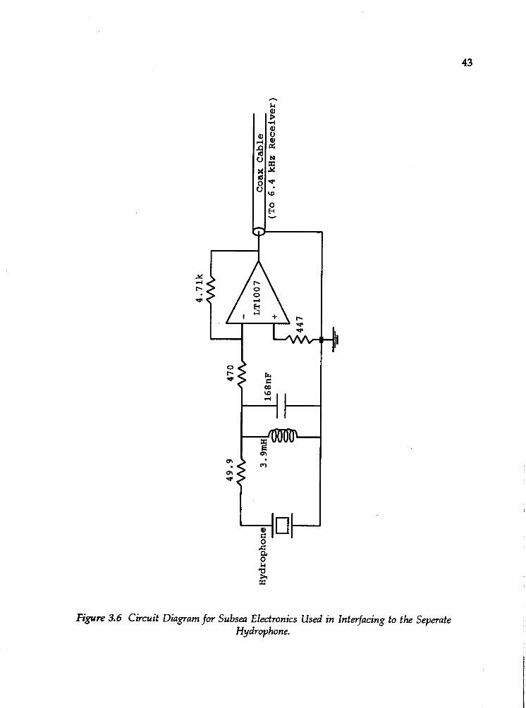
4.71k

49.9

Hyd

rop

hon

e C

oax

Cab

le

(To 6

.4 k

Hz

Rec

eiv

er)

0

44

used for reception. Also the series inductor was not necessary to improve the receive

response of the transducer. The preamp had a gain of 18.3 dB and a 39.0 dB rejection

of the 1 MHz carrier.

To evaluate a sonar system's performance, the amount of electrical noise must

be determined. This noise level is usually dominated by the preamp noise and

therefore must be calculated for the 6.4 kHz preamp circuits. Performing the

calculations on the preamp for the seperate hydrophone, the noise was found to be 15

nV /root Hz.

At the surface, the received signals are amplified, filtered and then rectified (if

desired) before being displayed with a digital storage scope. A number of attempts

were made to build such a receiver for the 6.4 kHz signal using an active sixth order

Chebyshev lowpass filter. This filter consisted of three Sallen-Key second order

sections which provided a gain of 46.0 to 66.0 dB at 6.4 kHz, a bandwidth of 8.6 kHz

and a 40.0 dB rejection of the 1 MHz signal. This circuit provided the desired receiver

characteristics, but it was too noisy because of the board layout. A four layer board

design, rather than the perf-board that was used, is necessary to reduce the noise to

acceptable levels.

To minimize costs and time, two of SMSL's receiver boards were modified for

use in this prototype. Block diagrams of the resulting receiver circuits for the 1 MHz

and 6.4 kHz signals are shown in Figures 3.7 and 3.8, respectively.

The 1 MHz signal is first soft filtered with a single stage tuned circuit and then

amplified with a variable gain stage. The resulting differential signal is mixed to 455

kHz, buffered to single ended and hard filtered with a 12 kHz ceramic filter. The

signal is buffered to differential again, amplified with another variable gain stage, and

then mixed to a 40 kHz carrier. Finally the buffered single ended signal is output,

both directly and after being full-wave rectified. Though this board was tuned to 1

MHz, the bandwidth was sufficient that both primary carriers were received and as a

result the observed receive signal had the characteristic beat pattern found when two

tones are summed. Further reduction of the bandwidth to eliminate this would have

required too large of a trigger pulse length.

For the 6.4 kHz signal, a baseband design was used and therefore the receiver

was simplified. The secondary wave signal is first soft filtered with a single stage

Figure 3.7 Block Diagram of the 1 MHz SMSL Receiver Board.

Figure 3.8 Block Diagram of the 6.4 kHz SMSL Receiver Board.

47

tuned filter and then amplified with a variable gain stage. The differential output is

buffered to single ended, filtered again with another single stage tuned filter, and then

buffered back to a differential signal. A variable gain stage is again used to amplify

the signal before buffering to single ended and then output, both directly and after

being full-wave rectified. The bandwidth of this receiver was measured to be

approximately 9 kHz.

For the purposes of this prototype, neither TVG nor AGC was necessary and

therefore a manually adjustable gain control was used. For each receiver board the

gain control was accomplished with two 10k ohm trim pots which independently vary

the variable gain amplifiers from -10 dB to +30 dB. A total gain of more than 100 dB

was possible on each board.

3.25. Primary Waves' Characteristics

With a completed prototype, evaluation of a large step-down ratio parametric

sonar system was possible. This section presents the beam characteristics for the two

primary waves which are important since they can directly affect the characteristics of

the secondary wave. The secondary wave characteristics will be presented in chapter

4 where the experimental results are compared to theoretical values obtained from a

computer model of the parametric array.

The first step in evaluating the primary waves was to determine their source

level which is a decibel measure of their acoustic pressure level relative to a plane

wave RMS pressure of 1 @a at a distance of 1 meter. The proper method is to

measure the acoustic signal directly with a calibrated hydrophone, however the only

calibrated hydrophone available was the Briiel & Kjaer type 8104 which has a

maximum calibrated frequency of a 120 kHz. The only other possibility was to

estimate the source level using the following sonar equation

where P is the transducer input power, q is the transducer efficiency, and DI is the

transducer directivity index. For a circular element, the directivity is determined from

where D is the element diameter, A is the signal wavelength in water, and the result is

expressed in decibels. The 1 MHz transducer in the prototype therefore has a

directivity index of 34.5 dB.

Measuring the voltage and current at the input to the transducer coax cable for

each transmitter in turn, the RMS electrical power into the transducer was determined

for each primary wave at three values of V, Using these values of power and the

transducer efficiency determined from the equivalent circuit model, the transducer

power output was determined. The primary wave source levels were then estimated

using the above equations and found to be nearly the same for both carriers. The

results presented in the following table are therefore those obtained for each of the

primary waves. Evaluation of the equations in section 2.2 verified that the effects of

nonlinear attenuation were negligible for a V, of 125 volts.

Table 3.1 Primary Wave lnput Powers and Source Levels.

VD (volts)

75.0

100.0

125.0

Electrical Power, P (watts)

227.2

343.5 227.9

4728 229.3

i

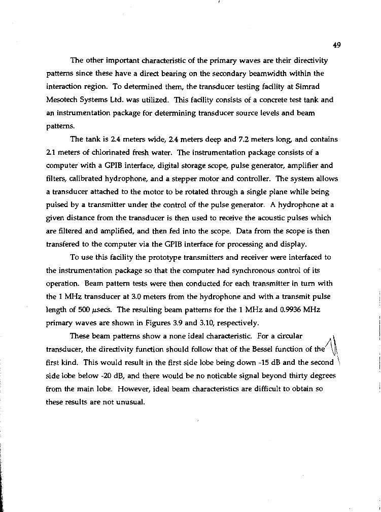
The other important characteristic of the primary waves are their directivity

patterns since these have a direct bearing on the secondary beamwidth within the

interaction region. To determined them, the transducer testing facility at Simrad

Mesotech Systems Ltd. was utilized. This facility consists of a concrete test tank and

an instrumentation package for determining transducer source levels and beam

patterns.

The tank is 2.4 meters wide, 2.4 meters deep and 7.2 meters long, and contains

2.1 meters of chlorinated fresh water. The instrumentation package consists of a

computer with a GPIB interface, digital storage scope, pulse generator, amplifier and

filters, calibrated hydrophone, and a stepper motor and controller. The system allows

a transducer attached to the motor to be rotated through a single plane while being

pulsed by a transmitter under the control of the pulse generator. A hydrophone at a

given distance from the transducer is then used to receive the acoustic pulses which

are filtered and amplified, and then fed into the scope. Data from the scope is then

transfered to the computer via the GPIB interface for processing and display.

To use this facility the prototype transmitters and receiver were interfaced to

the instrumentation package so that the computer had synchronous control of its

operation. Beam pattern tests were then conducted for each transmitter in turn with

the 1 MHz transducer at 3.0 meters from the hydrophone and with a transmit pulse

length of 500 psecs. The resulting beam patterns for the 1 MHz and 0.9936 MHz

primary waves are shown in Figures 3.9 and 3.10, respectively.

These beam patterns show a none ideal characteristic. For a circular

transducer, the directivity function should follow that of the Bessel function of the 4 first kind. This would result in the first side lobe being down -15 dB and the second ' side lobe below -20 dB, and there would be no noticable signal beyond thirty degrees

from the main lobe. However, ideal beam characteristics are difficult to obtain so

these results are not unusual.

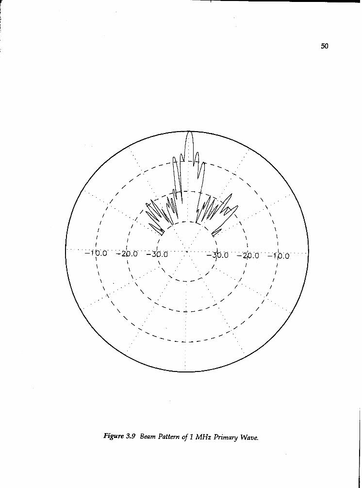
Figure 3.9 Beam Pattern of 1 MHz Primary Wave.

Figure 3.10 Beam Pattern of 0.9936 MHz Primary Wave.

References

Coates, R. F. W., Undmater Acoustic Systems, Halsted Press, New York (1989).

Konrad, W. L., Design and Performance of Parametric Sonar Systems, NUSC Tech. Report 5227, New London, CT (1975).

Konrad, W. L. and Carlton, L. F., TOPS, A High Power Parametric Source, NUSC Tech. Memo. TDlX-34-74, New London, CT (1974).

Berktay, H. O., Smith, B. V., Braithwaite, H. B. and Whitehouse, M., Sub-Bottom Profilers using Parametric Sources, Proceedings of The Institute of Acoustics, School of Physics, Univ. of Bath (1979).

Carl ton, L. F., Parametric Source Performance with Various Drive Wavej-orms, NUSC, Tech. Memo. #771155, New London Lab., New London, Connecticut (1977).

McMullan, B., Transducer Primer, URL Tech. Report (unpublished), Underwater Research Lab, Simon Fraser Univ., B.C. (1992).

Wilson, 0. B., Introduction to Theory and Design of Sonar Transducers, Peninsula Publishing, Los Altos, CA (1985).

Coates, R. and Matharns, R. F., Design of Matching Networks for Acoustic Transducers, Ultrasonics 26, pp. 59-64 (1988).

4. Secondary Wave Characteristics

As is the case with any sonar system, the beam characteristics of the projector

must be determined in order to evaluate the acoustic returns received by the system.

Theoretical models can be used to obtain the expected results, however these

generally vary significantly from the actual projector characteristics. This is even

more true of parametric arrays where the secondary wave characteristics are

dependent on the complex nonlinear processes of the water, and where theoretical

models can only approximate these processes.

This chapter examines the secondary wave characteristics of the large step-

down ratio projector used in the prototype. With one of the objectives of this thesis

being to investigate the use of this system for high resolution sub-bottom profiling,

the interaction region beam characteristics are of special interest, since higher lateral

resolution may be obtained by operating the sonar near the ocean floor. The use of

Muir and Willette's [4.1] volume integral, as presented in chapter 2, is therefore

used to obtain theoretical characteristics for this system. The experimental procedure

and results measured for the prototype secondary wave are then presented and

compared with the theoretical values.

For side scan operation of the parametric array, a secondary wave fan-beam is

required. This chapter therefore also presents the results from a computer model

which was used to investigate fan-beam characteristics within the interaction region of

the parametric array.

4.1. Circular Element Parametric Array Model As discussed in chapter 2, an interaction volume integral must be used to

obtain reasonable theoretical results within the interaction region. Muir and Willette's

[4.1] general secondary wave solution, equation (2.8), is therefore utilized. Using

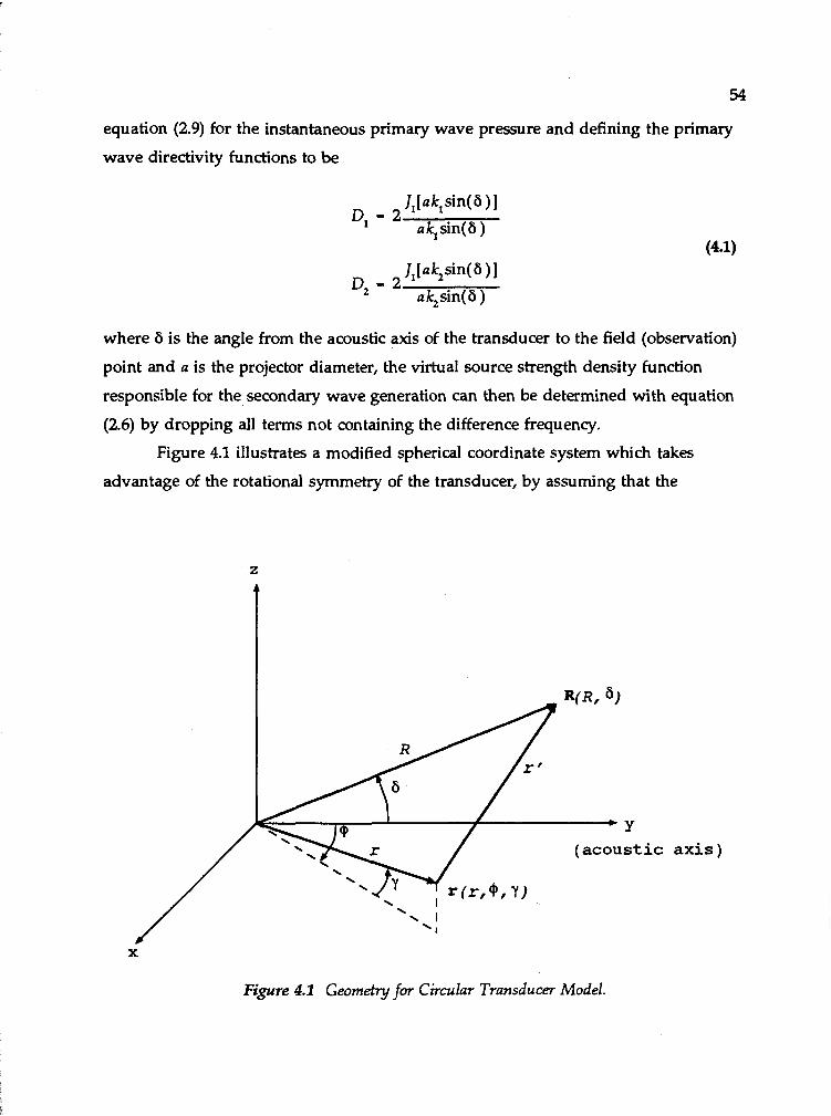
54

equation (2.9) for the instantaneous primary wave pressure and defining the primary

wave directivity functions to be

where 6 is the angle from the acoustic axis of the transducer to the field (observation)

point and a is the projector diameter, the virtual source strength density function

responsible for the secondary wave generation can then be determined with equation

(2.6) by dropping all terms not containing the difference frequency.

Figure 4.1 illustrates a modified spherical coordinate system which takes

advantage of the rotational symmetry of the transducer, by assuming that the

axis )

X

Figure 4.1 Geometry for Circular Transducer Model.

55

observation point, R is in the x-y plane. The circular transducer of radius a is located

in the x-z plane with its acoustic center along the y-axis. With this coordinate system

and suppressing the time dependence and harmonic terms, the expanded expression

for the secondary wave is

where, as a result of basic trigonometry,

r

and

This solution is valid for spherically spreading waves and should not include

the transducer nearfield. Therefore, the range integration was taken from the

nearfield distance, r, out to the range R of the field (or observation) point. The

nearfield (or Fresnel) distance is specified as

exp ' * -[(a, + a,) - jk]r + [as - jkS]r1

To minimize the necessary computations a maximum angle is specified on the

upper limits of integration for the two angles. These values are chosen to include a

significant portion of the acoustic energy radiated. Muir and Willette found that the

second null of the primary wave directivity pattern was adequate for good agreement

with experimental results. For the Bessel function of the first kind, J,(x) used to

express the directivity function for a circular element, the second null occurs when x =

7.01572.

The interaction zone had to be defined by discrete points because the volume

integral was calculated using a triple summation. A natural question then is what

resolution of source points within the interaction volume is required to produce

reasonable results? Muir and Willette, for primary frequencies of 482 kHz and 418

kHz and a transducer radius of 3.8 centimeters, used angle increments of 0.0006233

radians and a range increment of 0.1035 meters for tests up to a maximum range of

103.5 meters. This results in source points at the maximum range which are spaced

several wavelengths apart, however, their results agreed well with experimental data

that they collected. Good agreement occurred because, as Muir and Willette showed,

the secondary wave develops quickly within the interaction region where the source

points of their volume integral were much more closely spaced.

To verify this implementation, tests were conducted to reproduce the results

obtained in [4.1]. Using the same test parameters, secondary wave pressure values

were obtained for a variety of angles and ranges. These results were found to be

identical with those of Muir and Willette's.

With a working model of the secondary wave pressure within the interaction

region of a parametric array, theoretical results for the prototype could now be

obtained. All the parameters from the prototype can be inserted directly into the

model except for the peak pressures, p, and y,. These are obtained from the primary

wave source level calculations (see chapter 3), however the source levels are

referenced to 1 meter rather than Y, as required. To correct for this, the source level

must be translated to the nearfield distance assuming a spherical spreading law (I/?).

Using the 1 MHz transducer nearfield length, r, of 0.077875 meters the source level of

the primary waves, at the maximum V, of 125 volts, becomes 250.8 dB re 1 @a. The

peak pressure of the primary waves is therefore 3.467e+6 Pa. The range and angle

increments were chosen based on those in [4.1] and the fact that the difference

frequency wavelength here is 10 times that used in Muir and Willette's results. The

range increment chosen, therefore, was 0.01 meters and the angle increment was 0.006

rads.

The results obtained with this model using the parameters from the prototype

are shown in Figures 4.24.3 and 4.4. Figure 4.2 contains the theoretical source level

of the secondary wave. An interesting point about the secondary wave curve is that

it increases initially out to a range of approximately 0.8 meters where it begins

dropping off as the spreading losses become greater than the secondary wave

generation. The secondary wave source level then continues to fall off until its slope

is that of spherical spreading, as would be expected in the farfield of the array.

The theoretical beam pattern for this parametric array at 5 and 10 meters is

shown in Figure 4.3. This illustrates the desirable characteristic of no side lobes found

in all parametric arrays due to the exponential shading of the end-fire array. A

slightly wider beamwidth is obtained at the 10 meter range. Finally, Figure 4.4

presents the secondary wave beamwidths versus range. This curve illustrates how

quickly the array develops; minimum beamwidth is obtained within a few meters.

What is interesting is the increase in the beamwidth beyond 20 meters. Presumably,

the beamwidth continues to increase until it reaches the Rutherford scattering

beamwidth, equation (2.11), for the farfield of this array. This equation predicts a

farfield beamwid th of 9.4 degrees.

Experimental Results Experimental evaluation of the prototype was initially conducted in the Simrad

Mesotech Systems Ltd. (SMSL) test tank that was used to characterize the primary

waves (see chapter 3 for description). Source level data obtained from this tank

behaved oddly, however, and it was determined that the dimensions of this tank were

too small to allow for spherical spreading of the secondary wave. Since a sub-bottom

profiler would be used in open water where spherical waves would result, a decision

was made to use SMSL's covered barge.

>

Figure 4.2 Theoretical Source Lmel of Seconds y Wave.

Figure 4.3 Theoretical Beam Patterns of Secondary Wave at 5 and 70 meters (The Wider Beam is for a Range of 10 meters).

Figure 4.4 Theoretical Beamwidth of Secondary Wave.

61

This barge is moored at a local marina in approximately 14 meters of sea

water, and allows testing of the equipment in a real ocean environment. Two

problems that had to be dealt with at this site were noise, which was substantial at 6.4

kHz, and several hundred fish fry that were present when this data was collected.

The noise was of two types: boat noise that saturated the receive electronics when

ever a boat drove by, and a constant background noise which appeared somewhat

periodic in nature but was very non-stationary. Averaging of two or more receive

pulses on the scope reduced the effects of this background noise. For fish fry directly

inline with the projector and hydrophone the source level of the secondary wave was

found to be drastically reduce, however if there were only a few fish or if they were

at the outer extremities of the interaction region then an increase in the secondary

wave source level and beamwidth was observed. Employing mad fits of jumping and

banging was effective in terrorizing these fish fry.

Figure 4.5 Received Pulse for Prima y Waves.

As examples of the typical signals generated by the prototype, Figure 4.5

shows the primary waves that were received with the 1 MHz receiver and Figure 4.6

shows the 6.4 kHz secondary wave pulse at a range of 10 meters. Both were

generated with a pulse length of 500 psec. The pulse for the primary waves illustrates

Figure 4.6 Received Pulse for Secondary Wave.

the amplitude modulation of the beating primary carriers.

Tests were conducted using the 1 MHz transducer for transmission and the

calibrated hydrophone for reception. The test procedure involved obtaining source

levels and beam patterns of the secondary wave for various distances between the

transducer and the hydrophone. Unlike the test tank, the barge had no

instrumentation package to measure beam patterns so the procedure was done

manually. These beam patterns were measured to an angular resolution of 0.5

degrees, and half power beamwidths were then determined from this data using

linear interpolation to calculate values between the samples.

Figure 4.7 shows the experimental beam pattern obtained at the barge for a

range of 10 meters. The theoretical beam pattern is also included and illustrates the

large discrepancy that exists between the theory and data. To try and understand the

cause of this, Figure 4.7 was replotted along with the beam pattern for one of the

primary waves. This plot is shown in Figure 4.8 and illustrates that the wider

secondary beam is due to the non-ideal primary beam characteristics, since the

secondary wave will exist at least everywhere that the two primary waves coexist.

This is quite apparent for the larger angles where the primary beam produces what

Figure 4.7 Theoretical and Experimental Secondary Wave Beam Patterns at 10 meters.

\ . 0 Secondary experimen al) I

, . 0 Secondary theore t~ca l \ - P r ~ m a r y /

\ . ' / 1. .

Figure 4.8 Theoretical and Expm'mental Secondary Wave Beam Pattern at 10 meters with Primary Wave Beam Pattern.

65

appears to be side lobes in the secondary beam pattern. These results demonstrate

the importance of the primary wave beam characteristics and their effect on the

secondary wave.

As a result of the non-ideal primary wave characteristics, discrepancies

between the theory and data for the source level and beamwidth measurements are

also expected. The wider bearnwidths have already been demonstrated in the above

figures, and because the wider primary beams reduce the directivity index of the

projector, and therefore its source level, the secondary wave source level will also be

significantly reduced.

The secondary wave acoustic axis source level plots are presented in Figure

4.9. Shown along with the experimental data are the theoretical curve for the

secondary wave and the measured primary wave source level assuming spherical

spreading. As expected, a large difference in source level between the theoretical and

experimental curves for the secondary wave does exist due to the wider beam of the

primary waves. The experimental data is approximately 18 dB below that of the

theory which makes for conversion losses of 81 to 86 dB rather than the

approximately 68 dB predicted by theory for the 1 meter range.

Another factor that has not been considered but would also contribute to this

large discrepancy between the theoretical and experimental source levels is the value

for the primary wave source levels. These were used in the computer model for

calculating the theoretical values and therefore they directly affect the results. Errors

in these source levels are possible, since their determination was based on

approximate calculations of the radiated power rather than measurements of the

acoustic intensity. If greater losses exist within the transducer than were accounted

for in the calculations, then actual source levels will be less and the theoretical values

closer to the experimental values. An idea of the accuracy of the primary wave

source level estimate is hard to determine without actually measuring the source level

in the water; however, experience with other transducers has shown that the source

level may be in error by as much as 3 to 6 dB.

The last data collected at the barge were the beamwidths versus range. These

data are shown in Figure 4.10 along with the theoretical curve and confirm the

expected wider beamwidths. These results demonstrate how quickly the array forms

Range (meters)

Figure 4.9 Theoretical and Experimental Secondary Wave Source Levels with Primary Wave Source Level.

o Experimental

3 4 5 1 00

2 3 4 5 1 0'

Range (meters)

Figure 4.10 Theoretical and Experimental Secondary Wave Beamwidths.

0 Experimental -Theoretical Spherical Spreading)

Theoretical Cvlindrical Soreadin01

Range (meters)

Figure 4.11 Theoretical and Exyerimental Secondary Wave Source Levels Obtained in Test Tank.

with the minimum beamwidth obtained in only a few meters. To reduce these values

to those of the theory, a larger projector should be made with careful attention to side

lobe control.

To illustrate the effects of the test tank, the source level data obtained are

shown in Figure 4.11. These results indicate that source levels continue to increase

out to a range of 4 meters, which is approximately 3 meters longer than for the data

collected at the barge. The small confines of the tank have reduced the secondary

wave spreading losses and this allows the source level to grow farther into the

interaction region. Modelling of this behaviour was done with the computer

assuming a cylindrical spreading law of l /d r for the secondary wave. This

theoretical result is also shown in Figure 4.11, and though the source level is again

approximately 18 dB greater than the experimental data, the curve agrees well with

the slope of the experimental data.

To accurately model the experimental results the actual measured primary

wave directivity functions (beam patterns) could have replaced the ideal primary

wave characteristics (sin(x)/x) used in the computer model. This would have

accounted for the wider primary waves and produced theoretical results that were in

better agreement with the experimental data. The problem with this was that

summation over an entire hemisphere would have been required. The computation

time required for the generation of the above theoretical data was already more than a

couple days, and hence summation of the hemisphere would have been impractical.

Therefore, further modelling of the secondary wave for the prototype was not done

and the work in the thesis turned to evaluating the prototype for use in sub-bottom

profiling.

4.3. Fan-Beam Design For use of parametric sonar as a sub-bottom profiler in a side scan

configuration, a secondary wave fan-beam is required. This section investigates a

rectangular projector using the computer program for the secondary wave model.

Beam steering of parametric sources is also discussed and it is shown how this

steering may be used in generating a fan-beam.

4.3.1. Rectangular Transducer

With conventional transducers, fan-beams are generated using a rectangular

element or an array of elements to produce a large aspect ratio transducer. This

results in a narrow beam in the horizontal plane and a wide beam in the vertical

plane as required for side scan sonars. Therefore, rectangular parametric transducers

will be examined first to see if similar beam characteristics are possible.

A study by Berktay and Leahy [4.2] included the effects of rectangular

transducer shape on the secondary wave beamwidth. Their conclusions were that as

the beamwidths of the rectangular transducer were increased, the difference frequency

wave source level was reduced and its beamwidth was increased above that predicted

by equation (2.11) of Westervelt's model. Hence, as the primary wave beamwidths

tend to zero, the secondary wave farfield behaviour is controlled mainly by the

Rutherford scattering term, while for larger primary wave beamwidths the geometry

of the interaction region predominates. However, though the beamwidth of the

primary waves does affect the secondary wave, the results clearly show that the

endfire effects of the array limit the ratio of the secondary wave horizontal and

vertical beamwidths. This effect is illustrated in [4.2], where a transducer with a

beamwidth ratio of 8:l was used to obtain a secondary wave beamwidth ratio of only

1:3. This work was based on a model for the farfield, and therefore these results are

only valid outside the interaction region of the parametric array.

To investigate the secondary wave beam characteristics within the interaction

region, where the sonar would be used for high resolution sub-bottom profiling, the

program employed to model the circular transducer was modified to account for the

rectangular aperture. This required that the directivity functions for the primary

waves be redefined and that a new geometry be defined (since rotational symmetry

no longer exists). The directivity functions are now of the familiar sin(x)/x, or SINC

function, typical for rectangular elements. These are defined for the two primary

waves as follows

The new geometry is illustrated in Figure 4.12.

X

Figure 4.12 Geometry for Rectangular Transducer Model.

axis )

72

Again, suppressing the time dependence and retaining only the difference-

frequency terms, the expression for the secondary wave pressure is

where the distance between the field and observation points is now

To verify this implementation, the computer model was run for a square

transducer with the same frequencies and dimensions as was used for the circular

transducer. Although the elements have different shapes, this only slightly affects the

directivity functions of the primary waves and therefore the secondary wave

beamwidths should be very similar. Integrating the source field angularly to the

second null of the directivity functions and radially to 10 meters, the secondary wave

beam characteristics of the two transducers were nearly the same.

With a working model of a rectangular transducer, the secondary wave beam

characteristics were determined for a number of element dimensions using primary

wave frequencies of 1 MHz and 0.9936 MHz, and a range of 10 meters. The results

are summarized in Table 4.1. With m held constant at 2.5 centimeters, and therefore

the nearfield length, Y, was also constant at a value of 1.66 meters, the secondary

wave vertical beamwidth was increased as the transducer half-height, n, was

decreased. However, the horizontal beamwidth also increases as illustrated by the

primary and secondary wave beamwidth ratios shown in Table 4.1. As an example, a

primary wave with a vertical beamwidth 16 times greater than the horizontal

73

Table 4.1 Secondary Wave Characteristics for Several Rectangular Transducer Dimensions at 10 meters.

beamwidth results in a secondary wave which only has a horizontal to vertical

beamwidth ratio of 1 to 3.38. This supports the results of Berktay and Leahy where a

similar behaviour was observed in the farfield of the array.

Source levels of the secondary wave were also calculated using the input

power of 472.8 watts (V, = 125 volts) from the prototype. The primary wave source

level of 229.3 dB re lpPa @ lm, however, cannot be used since the shape and size of

the element will affect the directivity index @I). Re-calculating the primary wave

source level for each set of transducer dimensions, the secondary wave SLs obtained

are shown in the last column of Table 4.1. These show the source level decreasing as

the aspect ratio of the transducer is increased, which again agrees with the data

obtained in [4.2] for the farfield.

Secondary wave beamwidths and source levels were also obtained at a range

of 50 meters and are summarized in Table 4.2. Comparing with values at 10 meters,

the source levels are found to decrease and the beamwidths increase. This is in

agreement with results for the circular element. What is interesting is that the

secondary wave beamwidth ratio and the source level difference between the square

element and rectangular element have both decreased at the longer range. At 50

Table 4.2 Secondary Wave Characteristics for Two Rectangular Transducer Dimensions at 50 meters.

Transducer Secondary Wave Primary and Dimensions Half-Power Secondary Wave (dB re (centimeters) Beamwid ths Beamwid th

(degrees) Ratios

Horiz. Vert. Primary Second.

5.31 1:l

0.15625 17.75 1:16

meters, where the interaction processes are nearly nil, the interaction region and

therefore the primary beam characteristics, has less of an effect and hence the

secondary wave characteristics are controlled mainly by Rutherford scattering.

A conclusion from these results is that large secondary wave beamwidth ratios

are not possible in either the interaction region or the farfield of the parmetric array.

At best, a vertical bearnwidth which is approximately 3 times that of the horizontal

beamwidth may be obtained.

4.3.2 Beam Steering

The results obtained earlier have shown that the shape of the interaction

region does affect the secondary wave characteristics; however, as seen with the

rectangular transducer modelling, both the horizontal and vertical beamwidths are

affected and this therefore limits the beamwidth ratio that may be obtained. Other

attempts at manipulating the interaction region, such as intersecting the two primary

waves at an angle, may shorten the interaction region and therefore increase the

secondary beamwidth but the endfire array effects will dominate and again limit the

beamwidth ratio.

An alternate approach may be to use beam steering. Berktay [4.3] in his

original work on parametric arrays suggested the possibility of having arrays of

parametric sources that could, as with conventional linear arrays, be steered by

applying a linear phase shift across the array. This technique has been shown to

work experimentally by both Smith [4.4] and Carlton [4.5]. The results of

[4.5] are particularly impressive, where the Naval Underwater Systems Center's

(NUSC) high powered Towed Parametric Sonar (TOPS) was used to steer its beam 23

degrees.

Beam steering of a parametric array could possibly be used to produce a

secondary fan-beam characteristic. This approach has been implemented with

conventional linear arrays where an "in-pulse" sweep of the beam is used to

effectively produce a fan-beam [4.6]. With parametric sources where the

secondary wave is generated through nonlinear interaction within the water column,

there is a concern that the sweeping of the beam will affect the primary wave

interaction and therefore the secondary beam. A study on the effects of mechanically

rotating a pulsed parametric source [4.7] have shown that if the frequency of

rotation of the source is small compared to the difference frequency, then there is little

effect on the secondary wave beam characteristics. This suggests that such a

technique may be possible for parametric fan-beam generation.

References

Muir, T. G. and Willette, J. G., Parametric Acoustic Transmitting Arrays, J. Acoust. Soc. Am. 52, pp. 1481-1486 (1972).

Berktay, H. 0. and Leahy, D. J., Fagield P a j m a n c e of Parametric Transmitters, J. Acoust. Soc. Am. 55, pp. 539-546 (1974).

Berktay, H. O., Possible Exploitation of Non-Linear Acoustics in Underwater Transmitting Applications, J. Sound. Vib. 2, pp. 435-461 (1x5).

Smith, B. V., An Experimental Study of a Parametric End-Fire Array, J. Sound Vib. 14, pp. 7-21 (1971).

Carlton, L. F., Electrical Reamsteering of the TOPS Parametric Source, NUSC Tech. Memo No. TD124-105-75, NUSC, New London, CT (1976).

Tucker, D. G, Welsby, V. G. and Kendell, R., Elech-onic Sector Scanning, J. Brit. I.R.E. 18, pp. 205-208 (1958).

Widener, M. W. and Rolleigh, R. L., Dynamic Eflects of Mechanical Angular Scanning of a Parametric Array, J. Acoust. Soc. Am. 59, pp. 260-263 (1976).

5. Sub-Bottom Profiler Design

To evaluate the performance of a large step-down ratio parametric sonar for

use in sub-bottom profiling, the sonar equations must be evaluated in much the same

way as for a conventional side-scan sonar [5.1],[5.2],[5.3]. With a sub-

bottom profiler, however, the medium parameters are further complicated by the

wa ter-sediment interface and the propagation of sound through the sediment.

This chapter examines the propagation of acoustic waves across a water-

sediment interface and incorporates the results into the sonar equations. The resulting

equations are then used to establish theoretic bounds on the capabilities of a

parametric sub-bottom profiler, both at normal and oblique incidence. Finally,

experimental results are shown which demonstrate the operation of the prototype.

5.1. Water-Sediment Interface Unique to the sub-bottom profiler is the propagation of the sonar signal across

a water-sediment interface. The water medium is generally well defined and, for

most cases, very consistent in nature. The sediment medium, however, is not.

Sediment can vary from course sand to silt with each having its own

characteristics and therefore very different densities, sound velocities and attenuation

coefficients. In addition, marine sediments may become heavily saturated with

hydrocarbon gases due to biological decomposition or as a result of discharges from

deeper gas and petroleum reservoirs. The addition of these gases results in

significantly higher attenuation levels in the sediment.

The interface itself is further complicated by its "roughness". The ocean floor

can vary from flat and smooth to rolling and rough. As a consequence, the acoustic

beam patterns and source levels may vary significantly in the sediment.

To simplify the analysis of the water-sediment interface, two assumptions are

employed. The first is that the interface is smooth and flat, and the second is that the

sediment is thought of as another fluid and therefore precludes any generation of

shear waves. This latter assumption is generally valid due to the sediment being

saturated with water.

Much work has been done, both experimental and theoretical, to study the

penetration of parametric beams across such interfaces. Though a general

understanding exists as to what occurs, the difficulty of the problem leads to very

complex models of the interface. For this reason, a simplified plane wave model is

presented that, as will be shown, is valid for either bounded beams incident at

grazing angles above the critical angle, or wide beams which are approximately

planar at the interface. To understand parametric beam penetration, a discussion is

then made on the phenomenon found for grazing angles less than and equal to the

critical angle. ina all^, an asymptotic solution for bounded beams is presented which

is valid in the farfield of the insonified aperture at the sediment interface. ,

5.1.1. Plane Wave Model

Rayleigh [5.4] presented the original theory of plane waves incident on a

flat fluid bottom, for which the boundary conditions require that the pressure

variation and the normal components of particle velocity be continuous at the

boundary. Hence the usual equations

and

where p, p, and p, are the incident, reflected and transmitted pressures; p, and c, are

the density and sound velocity for the water; p, and c, are the density and sound

velocity for the sediment (assuming uniform medium); and, r$ and 8 are the grazing

angles of incidence and transmission as shown in Figure 5.1.

Figure 5.1 Geometry of the Water-Sediment Intetface.

Solving equations (5.1) and (5.2), and letting s = p1c1sin(8)/p,~sin($), the

following expressions are obtained for the reflection and transmission coefficients

To account for attenuation in the bottom fluid, P. M. Morse substituted a

complex wave number in to the above derivations. Publication of this work was first

made by Mackenzie [5.5] and then later in more complete detail by Horton [5.6].

The following is a summary of the expressions obtained for this model.

The equations for the wave numbers for the two media are now

where pi is related to the phase velocity vi through

2n 0 p i - - - - A. v i

(5.7)

and a, is the attenuation of sound in the bottom fluid which has been shown by

Hamilton 15.71 to be proportional to the first power of the frequency for most

sediments. Additional definitions are the acoustic index of refraction

and the impedance ratio of the sediment to the water

Substituting these expressions into the original equations, the reflection and

transmission coefficients of equations (5.3) and (5.4) are now expressed as

To get a Snell's law for this interface such that the angle 4 in Figure 5.1 is a real

angle, Morse interpreted the wave front in the sediment as a surface of constant

phase. The resulting expression for Snell's law then is

where

and

5.1.2. Parametric Beams

As previously mentioned, much work has been done to understand the

transmission of bounded acoustic beams across water-sediment interfaces. Early

investigations looked at obtaining source levels and field patterns of these narrow

beams in the sediment. Muir and Thompson [5.8] examined this experimentally

while Jarzynski and Flax t5.91, and Horton [5.6] developed theoretical models to

predict these values. Of particular interest was the analysis of [5.6] which predicts

that for incident grazing angles below critical, the acoustic beam is displaced at the

interface and penetrates more steeply into the bottom than predicted with the above

plane wave theory.

Interest in this problem increased significantly with the publication of

experimental work by Muir et a1 [5.10], where 20kHz bounded beams generated

by both linear and parametric sources were used. The results show that both

parametric (2 degree beamwidth) and linear (10 degree beamwidth) beams follow the

plane wave theory very closely when the incident grazing angle is greater than the

critical grazing angle. However, for angles at and below the critical grazing angle, the

parametric beam was observed to propagate more steeply into the bottom and with

less attenuation than that of the linear source. In addition, at the critical angle a

displacement of the narrow parametric beam along the interface boundary was

observed before entering the sediment. None of these results for sub-critical

penetration are predicted by conventional plane wave theory.

As a consequence, a number of authors focused their attention on developing a

model which fully predicts this phenomenon. Berktay and Moustafa (5.111 and

Tjstta and Tjstta [5.12],[5.13] addressed the beam reflection/ transmission

problem, as had Horton [5.6], within the framework of linear acoustics. Tjstta and

Tjstta, however, included the diffraction effects due to the insonified area at the

interface. Their expressions, which are valid in both the near and far fields of the

insonfied aperture, provide good agreement with the experimental results from Muir

et a1 [5.10].

Another approach taken by Jarzynski and Flax [5.9], and Wingham

[5.14],[5.15] accounts for the parametric nature of the bounded beam.

Wingham, through theoretical and experimental work, documents that for sub-critical

grazing angles the parametric nature of the beam must be included to predict the

acoustic field in the sediment.

More recent works by Jensen and Schmidt [5.16], and Williams and

Satkowiak [5.17] support the findings of Tjratta and Tjratta [5.12],[5.13]. They

found that the transmission anomalies, sub-critical penetration and beam

displacement, are a consequence of the beam properties at the interface and not due

to the beam generation mechanism. In addition, diffraction is considered the most

important factor in determining the field within the sediment at low grazing angles.

Both of these works utilize a full wave-theory solution, obtained from the SAFARI

model [5.18], to provide theoretical pressure contour plots.

Even with the above results, there still exists some confusion about the

displacement of the transmitted beam. For example, there is an indication from

acoustic fields plotted in [5.12],[5.13] that the acoustic axis of the transmitted beam is

actually curved. Tjratta and Tjratta [5.19] explored this further and show that

there is a region, about 10 wavelengths beneath the interface, where the beam may

experience dramatic changes with forward or backward displacement. Beyond this

region, the beam is well formed, but its axjs may be more or less bent depending on a

number of interface properties.

The penetration of bounded beams (parametric beams) across a water-sediment

interface is obviously a very complex problem for which no model to date is fully

adequate. However, the general conclusions that emerge from these investigations

are:

1. For grazing angles above the critical angle, bounded beams (including

parametric beams) follow very closely to the plane wave theory.

2. For grazing angles at and below the critical angle, bounded beams (less

than 10 wavelengths in diameter at interface) penetrate into the

sediment more steeply than predicted by Snell's Law (for lossy bottom).

3. The transmission grazing angle is dependent on the wavenumber-beam

radius product that is calculated at the interface.

4. The transmitted beam experiences a displacement which is determined

by the grazing angle. This displacement may or may not occur at the

interface.

Given that the behaviour of bounded beams at the interface is complex and

not fully understood, if a performance evaluation of a parametric sub-bottom profiler

is to be made then some reasonable model of the beam penetration into sediment is

required. The infinite plane wave model described above is acceptable for beams

incident above the critical grazing angle. However, as shown in [5.10], this model

fails for other angles of incidence when the beams are bounded.

Tjstta and Tjstta [5.12],[5.13] have shown that their diffraction model agrees

quite well with the results of [5.10]. In addition, limiting this model to certain cases

provides very simple asymptotic solutions. For these reasons, this model is presented

and used in the profiler evaluation.

5.1.3. Asymptotic Solution for Bounded Beams

Tjstta and Tjstta [5.12],[5.13] derived a solution of the water-sediment interface

problem based on diffraction, from the insonified area at the interface, being the

dominant effect. Limiting the solution to the case of ka large (ka >> I), where k is the

acoustic wavenumber of the signal in the water and a is the radius of the incident

beam at the interface, the insonified area can be evaluated as an infinitely compliant

piston source with phase and magnitude shading as determined by the incident beam.

Furthermore, assuming that the observation point in the sediment is at a range of r >>

ka2/2sin$, very farfield, from the center of the spot allows additional simplifications.

The resulting solution, however, still requires a numerical integration unless the

complex pressure amplitude of the incident beam across the insonified area, q,', is

constant. If q,' = yo everywhere on the spot and zero else where, then the expression

for the transmitted pressure, in the plane of incidence, is

where T is the complex transmission coefficient derived in section 5.1.1, S is the

cross-sectional area of incident beam at the interface, and F(8) is the transmitted

directivity function.

85

For an incident beam of square cross-section (2u x 2u) the diredivi ty function is

where

and a is the radius of the -3 dB beamwidth of the incident beam. For a beam with a

Gaussian cross-section (parametric beams) the directivity function is

where N = 0.347.

Of particular interest is the transmission grazing angle. For Gaussian beams,

which have a single maximum in the sediment, this angle can be determined by

setting the derivative of the magnitude of F(8) to zero. This expression

is then used in a root solving routine to obtain 8 for a given value of 9.

5.2. The Sonar Equations To evaluate the performance of a sonar system, the sonar equations must be

evaluated [5.1],[5.2],[5.3]. These equations are the working relationships that tie

together the effects of the medium, the target, and the sonar equipment. Available as

design tools for the sonar designer, these sonar equations are at best guidelines, rather

than exact, due to the complexity of acoustic signal transmission through water.

For a sub-bottom profiler, the sonar equations are used in calculating the

source level and directivity of the parametric transmitter, spreading and attenuation

losses through the water, transmission losses across the water-sediment interface,

86

transmission and attenuation losses through the sediment, and the reflectivity strength

of the target. A return signal intensity is then obtained and, when compared to the

received noise, used in determining limits on such system parameters as range,

grazing angle, and buried depth of target.

The sonar equation for the received acoustic signal intensity of a monostatic

sonar is

where r, is the range from the source/receiver to the interface, r, is the range from the

water-sediment interface to the target, and RI is the received intensity expressed in dB

Sonar

( S L , OCV)

TL (rw H e i g h t ( H ) + A L ( r w )

Figure 5.2 Illustration of Sonar Equation Parameters.

87

re 1 kPa. Figure 5.2 illustrates the parameters of this equation. A discussion of the

sonar equations for each of the parameters in equation (5.20) are presented in the

following sections.

5.2.1. Projector Source Level

The source level (SL) is expressed in decibels re 1 micro Pascal (pPa) at 1 meter) / and is a measure of the acoustic intensity output, at 1 meter, from a projector. For

linear sources the SL is usually measured at some distance greater than 1 meter and

then is refered back to the 1 meter reference by accounting for the spreading (usually

spherical, 1 /I-') los&In parametric sources, howeirei; fie source level doesn't fall-off

immediately but rather increases for some range into the interaction region until the

spreading and attenuation effects begin to dominate. At this point the SL gradually

decreases and eventually falls-off at the same rate as that due to the spreading loss.

Therefore, for use in the sonar equations the measured secondary wave source levels

have to be extrapolated out to the spreading dominated region of the parametric

array, and then the resulting value is refered back to 1 meter in the same way as for a

linear source. Calculating the SL in this manner assumes that the water-sediment

interface is at a sufficient range for the spreading loss to be dominant.

5.2.2. Spreading and Attenuation Losses

The spreading loss (TL) in both the water and sediment is the result of the

intensity of the plane wave spreading out in space as it propagates. In an unbounded

medium, the acoustic wave spreads out spherically and therefore the intensity falls off

as the square of the range. Expressed in decibels, the spreading loss is

The attenuation loss (AL) is due to the small signal absorption of the acoustic

signal in both the water and the sediment. In this analysis, the signal levels are

assumed sufficiently small that nonlinear attenuation can be ignored. Usually refered \

88

to as a, the attenuation is expressed in terms of decibels per meter. Thus, the

attenuation loss is

This value is dependent on frequency and the medium through which the acoustic

wave travels. In water the attenuation typically varies as the square of the frequency

while in sediment it varies as the frequency. For the low frequencies required for

sub-bottom penetration, the attenuation in water is almost negligible, however in

sediment it is very significant. Typical values of a at 6.4 W z are 3.2 dB1meter in fine

sand and 1.3 dB/meter in silt [5.2],[5.7].

5.2.3. Interface Transmission Loss

The interface transmission loss (PL) is due to the acoustic wave propagation

across the water-sediment interface. This loss is the portion of the incident wave that

is reflected rather than transmitted. Knowing that at the interface the intensities of

the incident, reflected and transmitted waves are conserved, 1; = I , + I , and that the

reflected wave intensity is given by

then the interface transmission loss is

For a monostatic sonar, where the transmit and receive transducers are in

approximately the same location, the reflected (return) signal from a buried object is

assumed to follow the same path as that of the direct arrival. As a consequence, the

interface transmission loss is the same for both the direct and return signals.

52.4. Target Strength

The target strength (TS) is a measure of the reflectivity and directivity of an

object or surface when intercepted by an acoustic plane wave. Expressed in decibels,

it is the ratio of the reflected intensity, refered to 1 meter from the target, to the

incident intensity for a given object. Typical values are 0 dB to -25 dB, however

values greater than zero are possible for large objects which focus the reflected

intensity. For the purpose of establishing limits on system parameters, the minimum

target strength expected for all targets should be used.

5.25. Open Circuit Voltage and the Return Signal Strength rr \J

The open circuit voltage (OCV) of the receiver transducer is a measure of the 1 transducer sensitivity. This parameter is expressed in decibels relative to 1 volt, and

is the voltage produced across the transducer (open circuit) when a plane wave of

RMS pressure 1 pPa is incident upon its face.

With all the sonar parameters defined, equation (5.20) can be used to

L.

\ determine the received signal intensity, RI (dB re 1 @a). h hydrophone is then used 1

to convert the received acoustic signal into an electrical signal. Using the OCV 1 1 (sensitivity) of the receive transducer the resulting output voltage can be determined

as follows

v output - lu + ocv

which has the units of dB re 1 volt.

5.2.6. Noise

There are two types of noise that may mask a sonar return signal: electrical

noise from the receiver electronics, and acoustic noise picked up by the receive

transducer. In order to determine the minimum return signal strength that can be

detected, the noise levels for both types must be calculated.

The noise from the receiver electronics is determined from the front-end

circuitry. Estimates of the front-end noise figure were presented in chapter 3.

For the low frequencies required for sub-bottom profiling 1 kHz to 20 kHz,

the average ambient acoustic noise, as shown in Fig. 7.5 of [5.1], is due to wind and

surface waves. Assuming the profiler will only be used in zero sea state conditions,

the following expression was determined as a ''best" fit of the noise spectral density

data

NSD - 44 - 18*10g(j)

where the frequency, f, is in kHz and the units of NSD are decibels per root Hz re 1

pPa. The actual noise level (NL) at the output of the receiver, however, is dependent

on two parameters. The first is the directivity of the receive transducer, DI, at the

frequency of the receive signal. The above expression assumes the noise is received

omnidirectionally, and therefore the use of a directional hydrophone will reduce the

received noise. The second parameter is the bandwidth of the receiver electronics. A

smaller bandwidth reduces the noise level, however it also limits the minimum pulse

length that can be received. A compromise is therefore required between the pulse

length of the transmitted signal and the noise level at the output of the receiver.

Using equation (5.26) and including the effects of the receiver bandwidth and the

directionality of the hydrophone, the noise level at the output of the receiver is

where BW is the receiver bandwidth in kHz and NL has units of dB re 1 pPa.

A final note about noise level, the above expression for noise spectral density

was for average ambient noise of deep water. For locations such as harbours and

inlets where high concentrations of marine traffic or industrial activities may exist, the

acoustic noise level can be up to 30 dB higher (see Fig. 7.7 of 15.11) than that predicted

by equation (5.27). This noise is highly variable and difficult to estimate without

actual measurements at the planned profiling site. For this reason, such noise will not

be included in this analysis; however, when evaluating a sonar's performance for a

specified profiling application, the presence of other noise must be considered and

accounted for in the analysis.

5.2.7. Reverberation

Like noise, reverberation is a corrupting influence which may mask sonar

returns. However, unlike noise, reverberation is a result of the transmitted acoustic

signal being reflected, or scattered, from objects or surfaces adjacent to the desired

targets. As a consequence, no increase in transmitter source level can reduce its

effects.

Two principal types of reverberation are volume reverbation, which is due to

objects such as fish or suspended particals in the water column, and surface

reverberation, which is due to scattering from the sea-surface or sea-floor. Of

considerable concern to the sub-bottom profiler is the sea-floor reverberation, or

otherwise known as bottom backscatter.

Up to now, the water-sediment interface has been assumed to be flat and

smooth, thus allowing simplification of the analysis. In actual fact it is quite rough

and therefore a portion of the reflected signal from the interface is directed back

towards the receiver. This bottom backxatter, if of sufficient strength, could be

mistakenly identified as a target or may actually mask the return from a target. Some

estimate of its strength is therefore required to determine the effect that backscatter

may have on the profiler's performance.

Typically, bottom backscatter is estimated using Lambert's law 15.11.

Assuming reflection from a unit area, this is expressed as follows

where + is the incident grazing angle and p is a proportionality constant which has a

value of l/x when all of the incident signal is reflected from the bottom. To account

for a portion of the signal being transmitted into the sediment, p has to be multiplied

by the squared magnitude of the reflection coefficient. Hence, the bottom backscatter,

in units of dB per square meter, is

5.2.8. Sonar System Evaluation

Using the sonar equations defined above, a performance evaluation of a sub-

bottom profiler can be made. This involves solving these equations for various values

of each design parameter of interest. Using some design criteria, the limits of each

parameter may then be obtained and a trade-off analysis between two or more

parameters may also be determined.

The criteria for determining these parameter limits is a minimum received

signal-to-noise ratio (SNR) for each of the acoustic and electrical noise. This minimum

SNR is typically calculated using a of probability of detection analysis, however for

the purposes of this thesis an SNR of 10 dB will be used as a reasonable lower limit.

Therefore, to determine the maximum range of the system, for example, the SNR

would be calculated for each of the noise types as the range is increased. The range

in which either SNR becomes less than 10 dB would then determine the maximum

range of the sonar system for the given set of parameters.

A further consideration is the target-to-reverberation ratio (TRR). As discussed

in an earlier section, the bottom backscatter may be a factor in detecting buried

objects, and therefore a comparison of its strength to the target strength should be

made. The target strength in this case must account for the fact that the target is

buried at a given distance below the bottom. This is done by adding the propagation

losses due to the sediment to the TS of the target.

The use of a spreadsheet is an effective way of solving the sonar equations to

evaluate the performance of a sub-bottom profiler. This allows the SNRs and other

intermediate calculations to be studied for a number of ranges. Figures 5.3, 5.4 and

5.5 illustrate an example of the spreadsheet used in the next section to evaluate the

sub-bottom profiling performance of the prototype described and characterized in

chapters 3 and 4.

The system parameters are defined along the top of the spreadsheet and

include those determined by the sonar equipment such as the frequencies, source

level, beamwidth, receiver bandwidth and noise, and receive transducer sensitivity

(OCV) and directivity. In addition, there are the parameters determined by the

environment and application of the sonar such as the water and sediment

characteristics, acoustic noise, minimum target strength, target depth, fish height, and

pulse length.

Below the parameters are several rows of intermediate calculations and the

SNRs. Each row is generated for a range as determined by the range index which is a

fraction of the maximum true range. As used here, the true range is defined as the

horizontal distance from the source to the center of the insonified spot on the bottom.

Para

met

ric S

onar

Des

ign

Wor

kshe

et

Fish

hei

ght (

m)

Max

. hue

rang

e (m

)

Freq

uenc

y. f

l (k

Hz)

Fr

eque

ncy,

f2 (

kHz)

M

ean

Frq

.. lo

(kHz)

Diff

. Fre

q..

fs (k

Hz)

Pu

lse

leng

th (s

econ

ds)

Bea

mui

dlh

(deg

s)

Bea

mw

idth

(rad

s)

Ran

ges

Ran

ge

ltu

e Sl

ant

inde

x ra

nge

rang

e (m

) (

4

Salin

ity (p

pt)

Pres

sure

(atm

) T

emp

(deg

C)

Rel

ax fr

eq. (

kHz)

A

lpha

, fo

(dB

/m)

Alp

ha, f

s (dB

/m)

Alp

ha, f

s, sed. (

dB/@

So

und

velo

city

, wat

er (m

ls)

Den

sity

, u%

ter (

kg/m

A3)

B

eta

of f

s, w

ater

(rad

slm

) So

und

velo

city

, sed

. (rn

ls)

Den

sity

, sed

imen

t (kg

lmA

3)

Bet

a of

fs,

sed.

(rad

shn)

Bol

tom

inte

ract

ion

Gra

zing

G

razi

ng

Bea

m

angl

e an

gle

wid

th

(deg

s)

(m)

35

Ban

dwid

th (k

Hz)

9

1 A

mbi

ent n

oise

58

.116

04

5

NL

(dB

re1u

Pa)

48

.116

04

Bot

tom

bac

ksca

tter

Rec

eive

r Gai

n (d

B)

Rec

dvn

Dl (

dB)

ocv

(dB

) Fr

ont-e

nd n

oise

T

otal

ele

c. n

oise

N

oise

(dB

re 1

V)

(dB

) T

arge

t dep

th (m

)

Pool

prin

t L

ambe

rt

Bot

tom

T

arge

t le

ngth

ar

ea

appr

ox.

scat

ter

reve

rb

(m)

(sq.

m)

(dB

1sq.

m) (dB)

ratio

(dB

)

Wat

er p

ropa

gatio

n (I

way

) ,

Sedi

men

t pro

paga

tion (

I-sa

y)

Atte

n Sp

read

T

old

Ref

lect

. In

terf

. Tx

Dist

anoe

A

tten

Spre

ad

Tota

l lo

ss

loss

lo

sses

C

oef.

Tx lo

ss

angl

e an

gle

loss

lo

ss

loar

es

(dB

) (d

B)

(dB

) (d

B)

(raW

(d

egs)

(m

eter

s)

(dB

) (d

B)

(dB

)

Aco

ustic

al

Ret

urn

SNR

Si

gnal

(d

B re

(dB)

lupa

)

Ele

ctri

cal

Furthermore, the actual one-way distance that the acoustic signal travels in the water

is called the slant range.

The footprint area calculation determines the size of the insonified area as the

pulsed signal intercepts the water-sediment interface. The width of this area is the

horizontal beamwidth at the interface, and the length, which is the distance in the

plane of incidence, is cclcos(+) where t is the pulse length, c is the sound velocity in

water, and + is the incident grazing angle. The maximum length is obtained at

normal incidence and is equal to the vertical (or cross-track) beamwidth, in meters, at

the interface. This insonified area is used to estimate the bottom backscatter and its

length determines the characteristics of the transmitted signal in the sediment. The

bottom backscatter is then used with the equivalent target strength at the interface to

get the target-to-reverberation ratio (TRR).

The total losses result is twice the sum of the one way water and sediment

propagation losses. These losses include the propagation losses in both the water and

the sediment due spreading and attenuation, as well as the interface transmission loss

(ITL). The sediment propagation distance is based on the transmission angle

determined from equation (5.19) and the specified penetration depth. This distance is

equal to the penetration depth for normal incidence and increases as the grazing

angle, and therefore the transmission angle, decrease.

Finally, the two SNRs are calculated. The first SNR is the ratio of the acoustic

signal to the acoustic (ambient) noise received at the hydrophone. The SNR in the

last column is the ratio of the received electrical signal to the electrical noise at the

output of the receiver electronics.

5.3. Performance Evaluation of Prototype To evaluate the prototype as a sub-bottom profiler the sonar equations

previously defined are used to establish limits on range and penetration depth for a

typical operational specification. Experimental results are then shown which verify

sub-bottom operation of the large step-down ratio parametric array.

5.3.1. Parameter Limits

To obtain limits on range and penetration depth, the spreadsheet described in

the previous section was used (see Figures 5.3, 5.4 and 5.5) with the system

parameters and secondary wave characteristics of the prototype. These values

determined from the prototype were:

SL (measured at 10m and refered back to lm) = 147.2 dB re lpPa

Beamwidth (at 10m) = 11 degrees

Pulse length = 500 psec.

Receiver bandwidth = 9 kHz

Front-end noise = 15 nV/root Hz

OCV (1 MHz transducer) = -208.3 dB

An operational specification was assumed for the sub-bottom profiler as follows:

Sonar height = 10 meters

Target strength = -10 dB

Water salinity = 35 ppt

Water temp. = 5 "C

Sediment attenuation (6.4 kHz, fine sand) = 3.2 dB/m

Inserting these values into the spreadsheet and using a desired target depth of 1

meter the spreadsheet results obtained are those shown in Figures 5.3, 5.4 and 5.5.

The graph in Figure 5.6 summarizes the SNR results obtained from the spreadsheet

and shows that for a minimum SNR of 10 dB that sub-bottom target detection is not

possible (at this target depth) with the current configuration of the prototype due to

the electrical noise. The SNR for the acoustic noise is shown to be approximately 30

dB higher than that for the electrical noise. This suggests considerable improvement

in performance could be made if the received electrically convert acoustic signal was

increased or that the receiver front-end noise was reduced. The electrical noise is

already quite low so increasing the receive transducer sensitivity would be the most

effective.

To observe the effect of increasing the sensitivity of the receive transducer, the

spreadsheet was re-calculated using the OCV for the 10 kHz transducer of the

prototype (see chapter 3). This transducer has a sensitivity that is 2A.8 dB greater

than that for the 1 MHz transducer. Figures 5.7 and 5.8 show the much improved

I -'Oo0.te I I I I

I 6 1'2 ' ' 18

True Range (meters)

I +- SignaVAcous. Noise -c SignaVElec. Noise + TRR 1

Figure 5.6 SNRs for Electrical and Acoustical Noise, and TRR (OCV = -208.3 dB).

True Range (meters)

I -m- SignaVAcous. Noise + SignaVElec. Noise +I+ TRR

Figure 5.7 SNRs for Electrical and Acoustical Noise, and TRR (OCV = -1 83.5 dB).

055 I

1 1.75 Target Depth (meters)

-m- SNR(elec.) = 10dB + TRR = 10dB

Figure 5.8 Maximum True Range versus Target Depth (OCV = -183.5 dB).

SNR due to the electrical noise. The maximum true range for a target at 1 meter

could be 10 meters, however if the TRR is taken as the limiting fador then sub-bottom

profiling is still not possible. The TRR curve in this graph also shows a sudden drop

near normal incidence. This occurs because as the grazing angle increases the length

of the insonified area also increases until it suddenly becomes equal to the beamwidth

at the interface.

Re-calculating the spreadsheet for several target depths and each time

determining the maximum true range for both a SNR (electrical) and a TRR equal to

10 dB, a trade-off analysis between the maximum true range and the target depth can

be obtained. This is shown in Figure 5.8 and illustrates the increased range for

shallower targets. These curves also show that the maximum depth at normal

incidence (maximum true range of zero) for detection of the target is approximately

2.25 meters, assuming that the TRR is not a factor.

To improve the TRR, either the equivalent target strength at the interface must

be increased or the bottom backscatter be reduced. Target strength is a fixed

parameter; however, bottom backscatter may be reduced by using a smaller secondary

wave beamwidth or a shorter transmit pulse. A pulse length of 500 psec was used in

the spreadsheet calculations. This corresponds to only three cycles of the difference

frequency and a shorter length would not be practical for penetration into the

sediment. The beamwidth, however, could be reduced by increasing the projector

dimensions so that the primary wave beamwidths were smaller. This actually has

additional benefits in that the larger dimensions would improve the transducers

sensitivity for reception of the secondary wave. Furthermore, from the model of the

water-sediment interface the transmitted wave was found to propagate more steeply

into the sediment when narrower beams were used. This would then reduce the

sediment propagation losses and therefore increase the equivalent TS at the interface.

Finally, these results do suggest that moderate gains in the area coverage rate

are possible by using the parametric array in a side scan configuration. Examining

the SNR limited results for the prototype using the 10 kHz transducer for reception,

the length of the insonified area is 20.2 meters. The secondary beamwidth at the

interface is approximately 1.9 meters wide, and therefore a 10.6 fold increase in the

coverage rate is obtained.

5.3.2. Experimental Results

To validate the operation of the prototype as a sub-bottom profiler,

experimental results were obtained. Ideally, controlled sub-bottom profiling

experiments in a test tank would have provided valuable quantitative results;

however, as was shown in chapter 4, the tank would have affected the results due to

the large wavelength of the difference frequency. In addition, the logistics of carrying

this out were prohibitive. Instead the "real" world environment of the barge was

again used and thus, due to the acoustic noise and variable conditions at this site, the

experimental results were limited to verifying that sub-bottom penetration and

detection of a target was possible with the prototype.

From the evaluation of the sonar equations, the performance of the prototype

using the 1 MHz transducer for reception was quite poor. Planned tests to detect a

pipe buried at 1 meter leaves very little room for error in the analysis. The

spreadsheet results for the 10 kHz transducer, however, show a larger error margin

for the SNR. Though the TRR curve is unchanged by using this transducer,

backscatter will not be a problem at normal incidence, or for modest grazing angles,

with a target depth of 1 meter. For this reason, the 10 kHz transducer was chosen for

reception of the difference frequency during the sub-bottom profiling tests.

A s was discussed earlier, a noise level of up to 30 dB higher-than the ambient

noise level used in the evaluation of the prototype with the sonar equations is

possible in harbours where marine traffic and industrial activities are present.

Experience obtained from measuring the prototype secondary wave characteristics

showed that this was the case at the barge, and therefore changes to the prototype

were required to improve the SNR for the acoustic noise. Increasing the transmitted

power would have required replacing the transmitters since they were outputting

maximum power already, therefore the noise level would have to be reduced. This

requires either a smaller receiver bandwidth or a larger receive transducer directivity

index. To keep the range resolution high, a longer transmit pulse was not wanted, so

the gain of the receive transducer was improved by adding a reflector to the 10 kHz

transducer. This results in a double gain in that the reflector focuses the transducer

towards the bottom, increasing its directivity, and therefore increases the receive

voltage and reduces the noise level.

This reflector had to have a diameter of more than a few wavelengths to

prevent aperture effects. For a 6.4 kHz signal this meant a diameter of over a meter.

To obtain such a large reflector, half of one of the large spheres that hang on power

lines to alert aircraft was used. These spheres are hollow fiberglass shells made from

two half spheres with an inside diameter of 1.3 meters. One of the half spheres was

then lined with thin neoprene to make it reflective and the cylindrical transducer was

then mounted at its center. The directivity of this transducer with this reflector

attached was estimated to be 24.8 dB. Therefore, there will be a 24.8 dB gain in the

receive voltage, Vmwt, and a 24.8 dB reduction in the acoustic noise. As a result, the

levels of the two SNR curves in Figure 5.7 will increase by this value.

The initial testing of the prototype involved the imaging of two pilings located

near the barge. This would confirm that the detection of two targets, seperated in

range by 0.8 meters, is possible and provide an opportunity to verify operation of the

parametric array with a pulse length of only 500 ksec.

Due to the layout of the barge, the projector was located 7.3 meters from the

first piling and the 10 kHz hydrophone was 5 meters behind the projector for a

Figure 5.9 Toy View of Site Layout for Piling Tests.

distance of 12.3 meters from the first piling. Figure 5.9 illustrates the layout of the

test site. The estimated propagation time of the pulse from projector to hydrophone

for the first piling was 13.2 msec using a sound speed of 1480 m/s.

Figure 5.10 shows the received pulses captured on the scope for a pulse length

of 500 psec. For all figures of the scope results, the trigger marker (T) corresponds to

Figure 5.10 Return Signal of Pilings.

the time of the transmit pulse or as a delayed version of this time. For the latter, the

trigger delay time is shown at the bottom of the figure. The single pulse shown on

Figure 5.11 Expanded View of Piling Returns for 500 P e c Pulse Length.

left of this figure is the direct arrival of the transmit pulse, and coincides with the

105

propagation time from the projector to the hydrophone. The double pulse is the

return from the two pilings. Using the cursors, the propagation time from the trigger

marker to the first piling return was measured to be 13.26 msec, as expected.

An expanded view of the piling returns is shown in Figure 5.11 and illustrates

an approximately 1 msec delay between the two pulses. This corresponds to the two

way travel time from the first to the second piling and agrees closely with the 1.08

msec time expected for a 1480 m/s sound speed. Figure 5.11 also shows that the

pulses themselves are longer than 500 psec. This smearing of the pulse is presumably

caused by multiple returns from each piling due to the penetration of the acoustic

signal into the wood.

Figure 5.12 Expanded View of Piling Returns for a 700 psec Pulse Length.

A 700 psec pulse length was also used and the piling return obtained is shown

in Figure 5.12. The two pulses now overlap and therefore prevent the two pilings

from being uniquely distinquished. This illustrates the improved range resolution

with shorter pulses.

Sub-bottom tests were then conducted in which a target was buried adjacent to

the docks near the barge. The target used was a 0.5 meter long PVC pipe with a 0.15

meter outside diameter, which should produce an estimated target strength of -11 dB

106

when insonified perpendicularly to its axis. This pipe was filled with rocks and

sealed shut and was then buried by a scuba diver using a high pressure water hose to

force the "fine" sand out from under it. A depth of approximately 0.85 meters to the

top of the target was obtained before difficulties with the equipment prevented

further sinking of the pipe. The bottom sand encountered in the excavation was

consistent in granularity throughout the volume to be insonified with the exception of

a few small rocks. This should result in uniform returns from the sediment and

prevent false targets from being detected.

Height (H)

Figure 5.13 Site Layout for Sub-Bottom Tests.

The prototype was set up on the floating dock above the buried pipe with the

projector and the hydrophone adjacent to each other and at a depth of 1 meter (see

Figure 5.13 for layout of test site). Two measurements were then taken with normal

incident insonification and a pulse length of 500 pec . The first was with the

apparatus directly above the target in 4.65 meters of water, and the second was with

the apparatus moved slightly to the side, in 4.76 meters of water, so that the target

was no longer insonified. The resulting sonar returns are shown in Figures 5.14 and

5.15, respectively, and clearly show that a target was detected.

Figure 5.14 Bottom Return with a Target.

Figure 5.15 Bottom Return without a Target.

In both figures a large pulse is received which corresponds to the bottom

backscatter return. The slight difference in peak amplitudes of these two returns and

the different trigger delay times used on the scope are due to the different water

depths. The clipping of these pulses was required so that the target return could be

easily seen. The target return in Figure 5.14 occurs approximately 1 msec after the

bottom return, which corresponds to a one way distance of 0.87 meters using a typical

sound velocity for fine sand of 1749 m/s. This result confirms the detection of the

buried target. Measuring the relative amplitudes of the backscatter and target returns

for a reduced receiver gain (i.e., no clipping of signals), the target reverberation ratio

(TRR) was estimated to be -4.4 dB. This is 3.1 dB more than the -7.5 dB predicted by

the sonar equations. The small pulse on the right side in Figure 5.14 was a random

noise signal that unfortunately was captured in this image.

Additional tests were attempted for oblique incidence sub-bottom profiling.

These involved moving the prototype off to the side and angling the projector and

hydrophone towards the target so that the pipe was insonified broadside. Several

locations and angles of the projector and hydrophone were used; however, no result

that confirmed the detection of the target was obtained. On a number of the

transmitted pulses a return corresponding to the target was received, but no

consistancy between transmit pulses was evident that would confirm the detection of

the target. Only at, or very closely to, normal incidence was this possible.

One explanation for this was the higher noise levels. Notably higher levels of

noise were obtained when the hydrophone was angled. This increased noise may

have been masking the target return that would have been smaller due to the oblique

incidence. Another reason was the difficulty in aligning the projector to target. For

the prototype's secondary wave beamwidth of 11 or 12 degrees, the diameter of the

insonified spot at the interface is approximately 1 meter. With the variable conditions

of this test site, the insonification of the target may have been difficult.

One final attempt was made at obtaining sub-bottom profiling results. A boat

was used to transport the prototype across to the other side of the inlet from the

barge where a large gas pipeline was known to be buried under the ocean. This pipe

had an approximate diameter of 1 meter and was buried under 1 to 2 meters of fine

sand. At the time of the test the water depth was 10 meters at the test site and there

109

was a slack tide. A chart recorder was brought along to record the results so that any

subtle returns that could have been missed with a scope would be seen. However,

only noise was obtained that had an amplitude which was greater than 20 dB that

observed at the barge. The noise had a similar characteristic to that seen in the other

tests which suggests the source was nearer. This would confirm the suggestion that

the intake pumps of the nearby thermal plant were the source of the noise that has

plagued the experimentation of the prototype.

References

I

I

I , , ' ' L A

Urick, R. J., Principles of Underwater Sound, 3rd ed., McGraw-Hill Inc, New York, New York (1983).

Coates, R. F. W., Underwater Acoustic Systems, Halsted Press, New York (1989).

Fox, P., Principles of Sonar Design, ENSC 894 course notes (unpublished), Simon Fraser University (1990).

Rayleigh, J. W. S. (Lord), The Theory of Sound, Vol. 11, 2nd ed., section 270, Dover Publications, Inc., New York (1945).

Mackenzie, K. V., Reflection of Soundfiom Coastal Bottoms, J. Acoust. Soc. Am., 32, pp. 221-231 (1960).

Horton, C. W., Sr., The Penetration of Highly Directional Acoustic Beams into a Sedimentary Bottom, Part I., Appl. Res. Lab. Tech. Rep. 74-28, Univ. of Texas at Austin, Austin, TX (1974).

Hamilton, E. L., Elastic Properties of Marine Sediments, J. Geophys. Res., 76, pp. 579- 604 (1971).

Thompson, L. A., and Muir, T. G., Narrowbeam Sound Fields in a Sand Sediment, Appl. Res. Lab Tech. Memo 73-36, Univ. of Texas at Austin, Austin, Tx (1973).

Jarzynski, J. and Flax, L., Penetration into a Sand Sediment of Diference-Frequency Sound Generated by a Parametric Array, J. Acoust. Soc. Am., 63, pp. 13651371 (1 978).

Muir, T. G., Horton, C. W., Sr., and Thompson, L. A., The Penetration of Highly Directional Acoustic Beams into\ Sediments, J. Sound Vib., 64, pp. 539-551 (1979).

Berktay, H. 0. and Moustafa, A. H. A., Transmission of a Narrozu Beam of Sound Across the Boundary Between Two Fluids, in Proceedings of the NATO Conference on Bottom-Interacting Ocean Acoustics, SACLANT ASW Research Center, Italy, June 1980, ed. by W. A. Kuperman and F. B. Jensen (Plenum, New York, 1980), pp. 259-284.

Tjstta, J. N. and Tjertta, S., Reflection and Refraction of Parametrically Generated Sound at a Water-Sediment Intoface, in Proceedings of the NATO Conference on Bottom- Interacting Ocean Acoustics, SACLANT ASW Research Center, Italy, June 1980, ed. by W. A. Kuperman and F. B. Jensen (Plenum, New York, 1980), pp. 239-258.

Tjstta, J. N. and Tjstta, S., Theoretical Study of the Penetration of Highly Directional Acoustic Beams into Sediments. 1. Acous. Soc. Am.. 69. vv. 998-1008 (1981).

[5.14] Wingham, D. J., A Theoretical Study of the Penetration of a Water Sediment Interface by a Parametric Beam, J. Acoust. Soc. Am., 76, pp. 11921200 (1984).

[5.15] Wingham, D. J., Pace, N. G., and Ceen, R. V., An Experimental Study of the Penetration of a Water-Sediment Interface by a Parametric Beam, J. Acous. Soc. Am., 79, pp. 363374 (1986).

[5.16] Jensen, F. 8. and Schmidt, H., Subcritical Penetration of Narrow Gaussian Beams into Sediments, J. Acoust. Soc. Am., 82, pp. 574-579 (1987).

[5.17] Williams, K. L. and Satkowiak, L. J., Linear and Parametric Army Transmission across a Watek-Sand Interface - Theory, Experiment, and Observation of Beam Displacement, J. Acoust. Soc. Am., 86, pp. 311-325 (1989).

[5.18] Schmidt, H. and Jensen, F. B., A Full Wave Solution for Proyagation 4n Multiluyered Viscoelastic Media with Application to Gaussian Beam Reflection at Fluid-Solid Interfaces, J. Acoust. Soc. Am., 77, pp. 813-825 (1985).

[5.19] Tjntta, J. N., Sagen, H., and Tj~tta, S., Transmission of a Sound Beam Across a Two- Fluid Interflzce: N u m h a l Results and Asymptotic Expressions, J. Acoust. Soc. Am., 85, pp. 2cQ-38 (1989).

6. Conclusions

Parametric arrays can produce a low frequency acoustic signal through the

nonlinear interaction of two high frequency carriers. This allows small transducers to

be used, particularly for a large step-down ratio, which makes them suitable for use

on ROVs. To better understand their characteristics and evaluate their use in sub-

bottom profiling, this thesis investigated a large step-down ratio parametric array.

A prototype of the parametric array was built using a 1 MHz ceramic disk.

Primary carrier frequencies of 1 MHz and 0.9936 MHz were used to produce a

secondary wave frequency of 6.4 kHz. Both the primary wave and secondary wave

characteristics were measured and a conversion loss of more than 80 dB was

determined, confirming the high losses typically associated with these parametric

arrays. Beamwidths of 10 to 12 degrees were obtained, however, for a transducer

with only a 2.5 centimeter diameter.

Computer modelling of the parametric array within the interaction region

provided valuable insight into the behaviour of these arrays. Large differences

between the predicted and actual secondary wave source levels and beamwidths were

obtained; however, the behaviour of both characteristics versus range matched very

well. The non-ideal primary wave characteristics were shown to explain these

differences, demonstrating the importance of the primary wave beams in determining

the secondary wave characteristics within the interaction region. Furthermore, these

results illustrated the limitations of the model due to the complex processes that exist

within this region.

Modelling the interaction region of parametric arrays with rectangular

apertures confirmed existing results for the fafield. Even with large transducer

aspect ratios, secondary wave horizontal to vertical beamwidth ratios of at most 1:3

113

were obtained. This limits the possible gain in area coverage rate if the parametric

array were to be employed in a side scan configuration.

Examination of the water-sediment interface revealed that a parametric beam

could penetrate the bottom at sub-critical grazing angles, and that it would penetrate

more steeply for narrower beams. Modified sonar equations were defined using this

interface model, and an evaluation of the prototype as a sub-bottom profiler showed

target detection was not possible. The combination of a low secondary wave source

level and a poor 1 MHz transducer sensitivity at the secondary wave frequency

limited its use to imaging of objects within the water column. However, when a

seperate hydrophone with a much larger sensitivity was considered, a bottom

penetration depth of over two meters at normal incidence was possible. Furthermore,

oblique incidence target detection could be achieved for a minimum grazing angle of

45 degrees.

Experimental results obtained with the prototype and the seperate hydrophone

verified that sub-bottom penetration was possible. Oblique incidence tests were

inconclusive due to the high levels of noise and variable conditions at the "real world"

test site, however detection of a buried pipe at a depth of 0.85 meters was confirmed

for normal incidence.

This work has shown that high step-down ratio parametric arrays can be used

for sub-bottom profiling, though the large conversion losses limit their use to near

normal incidence. Future work recommendations therefore include reducing the

parametric array step-down ratio to improve the source level and sensitivity of the

array, and further investigation of oblique incidence bottom penetration. Finally, the

problem of backscatter interfering with sub-bottom returns must be considered,

particularly at low grazing angles.