An Investigation of the Relationship between Business

and Financial Risk using Target - MOT AD: A Case

Study in the Victorian Mallee

Robert J. Cumming and Kevin A. Parton

Department of Agricultural Economics and Business Managetmnt

University of New England

Annidale NSW 2351

Paper presented at the Australicm Agricultural Economics Society Annual Conference,

University of Queensland, Brisbane, 13-15 February, 1990.

2

1 . Introduction

The relative contribution of fmancial risk and business risk to overall riskiness of a fann-fum has become a more significant issue in the Austtalian wheat industry recently.

On the financial side. the reasons for this include financial deregulation, which has enabled

fanners effectively to draw debt finance from a wider, more competitive market; and

higher intetest rates, which increase both the costs of debt fmance and the likelihood of

being unable to service the debt On the business risk side there are the continuing inherent

production and price risks of farming operations, and in addition panicular current

uncertainties concerning deregulation of wheat marketing.

It was in this environment that the issue of the impact of debt financing on our case­

study farm was analysed. This farm was a typical cereals-mixed livestock enterprise in the

Mallee in Victoria. The objective was to investigate the nature of the trade-off between financial risk and business risks in a total risk management approach to fann planning. The

influence of fixed financial obligations on the production mix of fnnn enterprises was of

particular interest.

The study is in line with Powell's (1987, p 6) thoughts that "Researchers can

perfonn an independent and complementary role in the development and evaluation of

finance products and plans, the development of suitable PC models for evaluating

alternative finance plans and the relative cost of alternative ways of managing and sharing

risk." Powell (1987, p 11) also notes that the discussion of future research issues should

be directed "particularly for research in the area of the provision of rural finance and farm

financial and risk management. II

To achieve the above objectives the method applied was to:

(a) identify the efficient set of risk management strategies from alternative cropping

and livestock activities,

(b) compare the effects of various levels of financial obligations on risk-efficient

sets, and

(c) describe the distributions of returns associated with optimal high and low risk

strategies.

3

Particular attention was given to the importance of downside risk. It is under a

threat to fann survival that the issues addressed in this study are of most importance to

fanners, the finance industry and to policy makers.

2. The Case-Study Fann

The case-study fann in the Mallce and the Mallee district in general are historically

highly dependent on wheat The overall short-tenn economic outlook for wheat fanners is

good, with this season's higher expected prices attributed in part to low production and a

depletion of stocks in the United States (U.S.D.A. 1989l!) due to a serious drought.

Despite the short-tenn outlook, considerable servicing of debt is still required and the long­

tenn outlook is not as promising. A considerable threat to future returns from wheat is

posed by the European Economic Community which is expectP..d to export an additional

eight and a half million tons in 1989 (U.S.D.A. 1989h), and the likelihood of the U.S.

rejoining the competitive export market Other threats to fann returns include the 4.4 per

cent decline in Australian agriculture's tenns of trade to the year ending March 1989. The

substantial inLTeases in interest ratest fann cost inflation at 8.4 per cent and a 15 per cent

increase in fertilizer prices have created the sharpest price rises in the year to March 1989

(Cribb 1989). As a result many Mallee fanners are still faced with downside risk for their

farm businesses.

At 1456 hectares, me case-study farm is close in area to the average Mallee fam' .()f

1507 hectares (Hall 1988a, p.34). The twenty per cent clay-loam, sixty per cent loam, and

twenty per cent sandy loam soils, combined with an average rainfall of three hundred and

fifty millimetres, results in a typical district 'consexvative' stocking rate of between two and

two and a half dry sheep per hectare. The location of the fann is shown in Figure 1.

Water supply for stock is adequate with good dams servicing the three blocks

making up the fann. The three blocks are separated by approximately five kilometres.

Shedding and silos on the two larger blocks results in no shortage of shed or storage space,

while sheep yards exist on each block. Facilities on one block such as the shearing shed

_'mp of Victoria

Figure 1 Location of case-study farm.

5

can service the'; whole fann. Established sheep handling facilities are typical of fanns in the M.allee.

Attention was directed to the MalIee because our a priori expectation was that debt

financing would be an issue there. particularly on cereals-mixed livestock fanns. Tables 1

and 2 show the fmancial risk status of different types of fanns, and reveal that cereals and

cereals-and-livestock fanns have incurred the largest amount of debt fmance.

3. Theoretical Background

The method adopted was to assess the risk-return trade-off at various levels of

threat to survival imposed by the obligation to meet debt repayments. In this context,

financial risk is defined as the added variability of the net cash flows relative to owner's

equity that results from the fIXed fmancial obligation associated with debt financing

(Weston and Brigham 1978). Financial risks expressing the cost and availability of credit

are reflected partly in interest rates for loans and partly through non-price sources. Non­

price sources include differing loan limits, security requirements, loan maturities, loan

supervision and documenta~""n (Barry 1983),

Business risk is the inherent uncenainty of the fann business resulting from

production variability and input and product price uncertainty. Uninfluenced by the

method{s) of finance, business risk is commonly defined by the coefficient of variation

Salrat when the expected net operating income is ra and the standard deviation is Sa.

Total risk (fR) faced by the farm firm is then the product of business risk (BR) and

financial risk (FR) when risks are measured in terms of coefficients of variation.

(l) TR = BR '" FR.

It has been hypothesised (Gabriel and Baker 1980) that farmers adjust the

production mix and pricing methods in order to reduce business risk when they are faced

with greater financial risk and vice versa. A change in the business or financial portfolios

may arise as a compensatory action to cope with a forced change in the other portfolio in an

attempt to keep total risk stable.

6

Table 1

Selected Faun Data for Different Australian Rural Industries 0985-86 dollars>

Farm

Farm Fann Liquid Fann

Capital Debt Assets Income

Wheat and other crops 675620 126590 411240 -70

Mixed livestock and crops 669620 79270 28420 11520

Sheep 624100 76100 26820 14840

Beef 761800 44410 45230 14560

Sheep-Beef 737 120 73530 27650 22140

Dairy 441370 49450 12670 18340

Horticulture 176370 28760 16340 18680

Total Agriculture 685910 79970 33870 11 320

Source: Hooke 1988

I >

I

7

Table 2

FjnuncjnJ Ri~k Status pC Sank Fuods t&Qt t9. Bmwcre farmers as Ass~s~eQ by their Banks a (Pr2PQ11iQn of Customers in kach Brgadaqe Industry Late 1987)

..... ~,-- FimUl9AI Ri~k ~iQll h_ I 2 3 4 5 Total

% ~ ~ 29 ~ %

Wheat and other cereals and mixed livestock 8.9 5.8 14.5 56.3 14.6 54.2

cereal gTains.

Sheep and mixed sheep-meat cattle. 2.3 2.2 6.S 68.4 20.4 27.0

Meat Cattle 2.4 2.3 6.4 71.9 17.1 18.8

All Broadacre 5.9 4.2 10.9 62.5 16.6 100.0

Source:Powell 1987, p.63.

a Includes 7 banks (Australia and New Zealand Banking Group Ltd .... Commonwealth Development Bank of Australia, Commonwealth Bank of Australia. National Austmlia Bank Ltd .• Rural and Industries Bank of Western Australia, State Bank

of Victoria & Westpac Banking Corporation).

b Category 1 Insolvent, no chance of recovery, classified as bad and doubtful debts. tI

II

..

2 Insolvent .. but can be kept fanning. loss of principal becoming apparent. 3 Problem accounts, no loss of principal or interest ex.cept in the short term (12 months).

4 Viable (borrower) .

5 Debt free (d.epositor only).

8

Empirical evidence to support the hypothesis of Gabriel and Baker has been

produced by Gabriel (1979) and Pederson and Bertelsen (1986). Gabriel looked at the

fnancial responses to changes in business ri~k on Central Dlinois grain fanns. Results

showed a substantial effect of financial risk upon modification of business risk. In addition

the impacts were found to vary between the different groups of fanners categorised

according to their level of risk aversion.

For a North Dakota fanner, Pederson and Bertelsen (1986) examined the 'trade off

between paying off the farm debt as quickly as possible to reduce financial risk (Le.,

reducing the level of fIXed financial obligations) and spreading business risks through

diversification of enterprises (i.e., adoption of flexible strategies). They also considered

the impact on the fann activities selected of a shift from share renting (low financial risk) to

cash renting (higher financial risk). Again a relationship was found to exist between the

portfolio of fann business enterprises chosen and the extent of fixed financial obligations.

Barry (1983), in his extended portfolio model, modified t~e above formula to

produce equation 2.

(2) TR = (Sa/ Rn) * {Ra Pa I (Ra Pa - Id Pd)}

where Sa is standard deviation of return on risky assets,

Ra is expected return to the risky assets,

Id is interest rate on debt,

Pa is proportion of risky assets in the portfolio, and

Pd is proportion of risk-free asset (debt) in the portfolio.

TR is total risk

According to Bany~s model, percentage h ....... eaS:;;:s in business risks are expanded

by percentage increases in financial risk through increased leverage. "Since variability of

returns to assets (S.) and the index of fmancialleverage (Pd) are both positively related to

the level of total fann risk, a strategic trade-off could occur between financial management

strategies which modify business risk exposure and scale adjustments in leverage"

(Pederson and Bertelsen 1986, p. 68).

9

The final tenn of equation 2, which measures the coefficient of variation of financial

risk, is the ratio of (a) total expected retums to the risky assets to (b) total expected returns

to the risky assets less total cost of debt Importantly, the size of the multiplicative risk

effect caused by this tenn depends on the denominator, which measures the amount by

which expected return 011 business assets exceeds the cost of borrowed funds.

In the case-study analysis, particular attention was paid to downside risk, and a

Target-MOT AD model was developed to cope with the threat to fann survival from the

uncertainty associated with achieving a minimum net operating income. This was

considered to be the most appropriate analytical technique as it is under a fann survival

threat that increased consideration would be given to the relationship between business and

fiMnce portfolios. It is also in this environment that the relationship will be of importance

to policy makers, finance companies and farmers. The safety-first criterion (Pyle and

Turnovsky 1970) included in the Target-MOTAD model is considered a suitable method of

analysing risk responses of farmers concerned with fann liquidity and survival.

This model has its roots in the mean variance (E-V) analysis developed in the 1950s

(Markowitz 1952, Tobin 1958), and many commen~'ies have been made about its

suitability as a decision criterion (Tsiang 1972, 1914). The optimal solution to an E-V

problem can be obtained using quadratic programming. Meanwabsolute deviation analysis

or MOTAD is a linear technique designed to approximate this quadratic res,llt (Hazell

1911). MOT AD is built on the assumption that risk is perceived as the absolute deviations

from the mean. Unlike the quadratic programming technique of E-V analysis in which

deviations are squared, larger deviations are not given extra weight with mean-absolute

deviation analysis. Originally MOT AD was developed to accommodate the shortage and

cost of computer power. As computational cnpacity has increased over time, however, so

have the applications suitable to MOT AD and variations of MOT AD.

Adaptations of the above two efficiency criteria, which account for the safety-first

approach inolude those by Porter (1974), Tauer (1983), and Watts, Held and Helmers

(1984). Porter developed a target-semivariance (T-SV) analysis while the remaining

authors were involved in the development of a target-negative deviation (T-ND) approach.

Target-semivariance analysis assumes that decision makers perceive risk as

deviations below a critical, target level of income. The squaring of deviations below the

target level results in quadrntic progrnmming being used~ as in E· V analysis, so that l~.rger

10

deviations are given more weight (Bertelsen 1985). Larger deviations below the mean are

therefore penalized more than smaller deviations implying that the assumption of decreasing

absolute risk aversion is 'buill in'. However, decreasing absolute risk aversion is unlikely

to be an imponant infiue,nce in a time of economic hardship. and need not be used as a

justification of target .. semivanance analysis (T-SV). The use of quadratic programming

requires a covariance-semivariance matrix to be specified. This involves a necessary level

of data ac(..~mulation uncharacteristic at n fann level.

In contrast, target-negative deviation (1' -NO) analysis can be solved using linear

programming. The analytical technique is given the name 'Target-MOTADt• The risk

constraint is the probability weighted sum of deviations below the target income level

(Bertelsen 1985).

The target .. negative deviation approach seems the most suitable, time .. and-cost

efficient method of deriving the efficient set of fann plans under the target income level

restri<..1ion. The deviations from the mean are not squared. so that the Target-MOT AD

approach does not require a covariance-semivariance matrix and the detailed infonnation to

create it; the lower amount of specific fann level data is more readily obtained given that

this constraint does not exist "No numerical index of risk preference is required in T-NO

analysis. The level of constraint on negative deviations from target is inversely related to

the degree of risk aversion. The risk-efficient set of actions is derived by maximizing

expected income at varying levels of risk constraint. A trade-off occurs between expected

income and deviations below the target income levert (Bertelsen 1985, p. 15 ).

Fishburn (1977) demonstrates that target-negative deviation analysis produces an

efficient set which is a subset of the second degree stochastic efficient set Stochastic

dominance (Anderson, Dillon and Hardaker 1980) is a preferred efficiency criterion of

many purists of decision analysis. Empirical studies (Porter and Gaumitz 1972. Anderson

and Lionardi 1982) and the analysis o·f Porter (1974) also suggest that other moment based

methods are suit:lble low cost instruments for obtaining efficient sets. Results from the

moment based target-negative deviation analysis are therefore considered reliable estimates

from which inferences can be drawn.

11

4. PThe Model

The Target-MOT AD model used in this analysis examining trade-offs between

business and financial risks is represented by the following system.

(3) Maximize E(R) X = R X (3.1)

Subject to: A X < B (3.2)

Rite X +d- > T (3.3)

Pd- < D (3.4)

X, d > 0 (3.5)

R = 1 x n vector of expected returns for each activity;

X = n x 1 vector of activity levels;

E = expectation

A = k x n matrix of resource requirements;

B = k x 1 vector of resource constraints;

R· = series of 1 x n vectors of expected net returns;

T = m x 1 vector \\ith each element equal to the target;

d- = m x 1 vector of negative deviations from target;

P = 1 x m vector of probabilities for each observation (i), Pi= 11m;

D = a scalar parameterised from zero to a large number;

n = number of activities;

m = number of observations, (simulated years); and

k = number of constraints.

Equation 3. 1 is the specitication of the objective function used. Revenue

ma.ximization, whil! not the only measure of a fanner's success, is of particular importance

in the context of a threat to fann survival, which is the context assumed for this

examination and on which the model is constructed.

Resource C< Instraints are specifieo by equation 3.2. Land, labour, and feed

availability are the I· mited resources to be considered.

12

In equation 3.3, the deviation from the target level of income is defined as 'd-'.

The sum of the simulated net revenues (R*X) and the pemlitted number of deviations (d-)

must exceed the target income level (T). The pennitted number of deviations in equation

3.3 is deftned according to equation 3.4 in which the probability weighted sum of

deviations (Pd-) must be less that the defined acceptable deviation from the target (D).

Parameterisation of D provides the risk-efficient frontier.

Table 3 is a schematic matrix of the linear programming model used. Linear

resource constraints which are binding on the fann operations are represented

mathematically in the fIrSt set of rows of the matrix (ROt to ROk in Table 3). The entries

Rt,l to Rso.I0 are 50 simulations of net revenue for each of the production activities. Then

each of the constraints aBSI to OBSso has an associated target income (f) shown in the

right hand side. If the difference between the sum of the revenues of the enterprises in the

basis and the target income is negative, then deviation activities enter the solution (DEV 1 to

DEVso). Finally, the row labelled SUMDEV accumulates the negative deviations and

weights them by their probabilities (PI to Pso), equal to 0.02. By parameterising the right

hand side of this matrix for a given level of target income, different basic solutions to the

target-MOT AD problem are obtained, each varying according to the probability of

achieving a given target income. The series of solutions from such a paranleterisation is the

risk-efficient frontier.

5. Data

The data set for this model can be categorised into the three areas of production

constraints, the target income, and simulated net revenues and objective function.

5.1 Production constraints

The land and capital constraints were treated together. The property size is 1,456

hectares. Ten hectares are assumed to be used for roads, houses, sheds, wind breaks and

fence lines. To cope with the fann decision maker's preferences, limits were placed on the

number of hectares which can be allocated to the production of wheat, barley and peas.

Such limitations help cope with barley's timeliness-of-harvest requirement; barley will

damage more readily than wheat and has ?-. ·;horter optimal time before it lies flat, sprouts or

drops to the ground. The area allocated to peas is limited to cope with the specific disease

problems which could build up if the area of peas in a crop rotation is enlarged. Similarly,

13

Table 3

Schematic Tableau of Target MarAD Model

RQ~ frody£tion A~1ivitiS(~zmz"IUQlh~r A£tivi1i~~ I&v 1 u.u:o.o:D~v~Q OBI SRI ER2 ER3 ...... ERI0 ROt ...... ~ _ ............... -ROt ...... - _ . ., ........ _ .. -

ROk ...... - _ .............. -OBSI Rl.I Rl.2 RI.:! ...... Rl.lO 1

........... ,. .

.............

.............. OBS50 RsO,l R50,2 Rso.3 •.•.• RsO.IO 1

SUMDEV El P2,o:, O ,Z-:,,;PSQ

OBI is the objective function to be luaximised.

RHS is the right hand side for the resource restriction (B) or target (I).

INC is the increment by which the right hand side is parametelised.

B. Rand m are as defined in equation 3.1

RHS max Bl

B2

Bk

T

T D

P is 0.02 (11m) times the value of any negative deviation from the target income.

D is a parameterised value.

INC

-IQ

14

wheat's maximum area helps stop the build up of diseases such as Cereal Cyst Nematode

and Takeall. Medic pastures also break life cycles of grass-born diseases 1:.v it is assumed

that the area not cropped is given to medic pastures. Wheat, barley, ano peas are limited to

eight hundred, four hundred, and two hundred hectares respectively.

Turning to labour, in order to allow for the hours spent on general farm activities,

repairs, maintenance and other miscellaneous work, a total labour constraint was imposed.

The constraint is in the fonn of seasonal labour restrictions and allows for the fact that the

fann operator's wife is active in assisting with various activities. A 'hire labour activity

was included in the Target-MOT AD matrix to give flexibility with respect to labour ir

selection of optimal management programs, and account for the availaOility of casual labour

and the fann operator's willingness to use casual labour. Labour requirements specifit. tc

th{~ different activities defined for the fann were obtained from Department of Agriculture

fann management surveys of the region adjusted in consultation with the operator. They

are listed in Table A.I in the appendix.

In calculating feed availabilities, crop rotations bad to be considered to cope with

diseases such as Cereal Chit Nematode and Takeall as well as to maintain adequate soil nutrients. An assumption was therefore made that at least twenty per cent of medic

pastures will be in their fm t year. Another assumption with respect to feed availability is

that there is autonomous ftedproduction at a level of 0.05 Live Stock Months (LSM)

(Rickards and Passmore 1971) per hectare in Summer and Winter and that figure is

doubled in the Autunm and Spring. The autonomous feed production is designed to

account for natural grass gmnination and growth. Feed produced by various types of

pasture and crops and feed required by livestock were derived from White and Bowman

(1981) and Oram (1985). Appendix Table A.2 shows the actual levels of feed and feed

requirements.

No limits were placed on the number of sheep and cattle possible in the production

mix apart from those restrictions imposed L'1rough other constraints such as feed. It is

assumed that a reasonable spread of the work load associated with lambing will occur

because of the natural spread of lambing due to failures to conceive and the nonnallack of

synchronization of the oestrous cycles. Parasite control measures are assumed adequate to

cope with a laq,""e flock.

15

The preference of the farm operatoJ' is that there will be only one sheep breeding

acti\ ity in the production mix. No additional computations are needed to cope with this

preference as only one sheep activity enters any production mix in the results obtaL.l1ed.

~.2 1rar.getincome

The target income level cr in 1rable 3) is tbe amount required to meet the demands

for family consumption, fIXed fann costs and fIXed financial obligations. The target income

for the typical 1500 hectare MaUee wheat/sheep fann with a debt problenl can be fonnulated

according to the method in 1rable 4.

A broadacre fann, such as the case-study fann, under a threat to survival because of its financial position would typically have equity levels of 60 to 70 per cent (Burgess and

Came 1989). Given this range of typical equity levels and with the knowledge that

commercial interest rates have fluctuated significantly since the deregulation of the money

market, 1rable 5 was constructed. It outlines possible debt servicing obligations of a farm

under a threat to survival. The case-study property is believed to have a value of $625 per

hectare or a total of close to $1 million (Simpson 1989). A 10-year loan is assumed for the

debt outstanding with a one per cent margin placed on the interest rates between 17.75 and

21.75 per cent (Burgess and Carne 1989).

The three target incomes to be examined in this study, to express different fmancial

risks through different fixed financial obligations were therefore $107 000, $125 000 and

$145000. These target incomes cover a likely range of interest rates and fann leverage

situation.

5.3 Simulated net revenues and objective function

The objective function entty for each activity is the mean of the simulated net

revenues l:Rij/50. Hence by describing the estimation of simulated net revenues, the •

objective function is automatically considered. Each element (Rij) has a value equal to

revenue (pij Yij) minus variable costs (VCj), where pij is defined as the real effective

returns to growers per unit and yij the yield.

16

Table 4

.EQnnularion of Target Income

---------------------------------~--------------~$~-Family Living Expenses a Fixed Fann Costs b

wadministration

-rates

-insurances

6036

5622

3385

~m 1~5

-wages and COIltraCtS( autonomous) 3640 C

Fixed Financial Obligations d

-conli~rcia1 :aterest plus margin 68 268

-principai requirerl on twenty-year loan 16450

20000

20258

Mill. 124976

a Arbitrary figure approaching that necessary to support one household

on the case-study farm.

b Derived from Hall (19~~b)

c Casual labour assumed autonomous.

d Derivation given in cetril in Table 5

Table 5

Likely Debt Servicing Obligations

Equity %

(de btl

70 ($300 000)

65 ($350000) 60 ($400 QQQ)

Commercial Interest plus 1.0 % margin

18.75 % 20.75 % 22.75 %

67200

84700 104800

17

(3) Rij = pij yij - VCij

R = sitnulated net revenue p ::: price. y = yield.

VC = variable costs. i = 1 to 50 simulated obselVations. j = 1 to 10 production activities.

In general, subjective data were used for levels of yields and prices while objective data were used for variable costs and for estimating correlations in yields and prices. Incorporation of subjective beliefs of likely price and yield distributions is considered vital

for the analysis to accurately define the decision context of the fann operator. The

infonnation elicited from the fann operator was obtained in the form with which he was most familiar; in the case of yields, bags per acre were recorded and subsequently converted to lonnes per hectare. The approach of eliciting data in this way is consistent

with dealing with some of the problems highlighted by Anderson, Dillon and Hardaker (1980) regarding the elidtation of distributions. In an appeal to parsimony, triangular probability density functions of yields and prices were elicited from which cumulative distributions were created and from which random samples were taken using a variation of

Monte Carlo random sampling. The above approach may go against the grain for purists of Decision Analysis, preferring a less definite ending to the cumulative distribution functions derived, but alternative methods of establishing cumulative distribution functions such as the juo.gmental mctile method (Anderson, Dillon and Hardaker 1980, p. 24) would have been too time consuming and were considered too testing of the farm operatorts

patience. The resulting distributions are shown in Table 6.

A complicating feature of the simulated net revenues is that there are correlations between the various activities in their yields and prices. Yield correlation is clearly existent

as the Malice is highly susceptible to climatic variations which affect all crops. To account

for this, historical yield infonnation generated by various trials conducted in the Mallee was used (see Cumming 1989 for details).

18

Table 6

Irlim&l!lm: ni~mtm1iQn~ Qf ProdU£Don A&nl1Ji~1

Activity Pri£~ Yi~ld

Mi!!imum MQSILik~l~ Minimgm MaximYDl MQ:ilLik~l! Minimum

Wheat 168.7 153.4 153.4 3.27 1.84 0.51

Malt Barley 200.0 180.0 170.0 1.93 1.23 0.35

Feed Barley 150.0 140.0 130.0 3.34 1.76 0.88

Field Peas 250.0 180.0 150.0 1.84 0.82 0.41

erl£~ Qf woo13r h~ad Pri£~ I!~r h~ 11Ul Qff

Wool/weth's 32.0 30.0 26.0

IX Lamb A 28.0 25.0 12.0 38.0

IX Lamb S 28.0 25.0 12.0 38.0

2XLambA 18.0 15.0 13.0 41.0

2XLambS 18.0 15.0 13.0 38.0

!:iW~ilnkr& 3~Q3Q

IX = first cross, 2X = second tross. A = Autumn drop lambs, S = Spring drop lambs.

wf = winter fatten. Yield in $ per hectare, Price in $ per tonne or $ per head.

30.0 20.0

30.0 20.0

29.0 20.0

27.0 20.0

3OO:Q 2aQaQ

19

Price correlation is believed to exist because of l<r-al and international

substitutability of grains. especially as stock feed. The historical price infonnation for

crops is contained in Appendix Table A.3. Because there are insufficient records, with the

current market structure. of the price of peas over time, peas are left out of the data used to

generate the correlatioJ matrix and a correlation with wheat of 0.25 is assumed. for the

modelling exercise reported in this study. A correlation of 0.25 reflects the comparatively

low substitutability of wheat and field peas due to their different protein contents and

different uses.

Correlations between wool prices and the prices paid for lambs should be

recognised. A correlation between firstkcross lambs and the price of wool was assumed to

be 0.3 and the correlation between second-cross lambs and the price of wool was assumed

to be 0.2. These figures reflect the intluence wool prices have on the willingness of

producers to pay for stock.

The localised weather patterns need not have any substantial effect on the local,

world dominated competition for grains, therefore at the fann level being considered in this

study, no price-yield conelations are incorporated

Net revenues for crops were obtained after subtracting expenses from the gross

revenues calculated by multiplying the 'price generated' with the 'yield generated'.

Expenses were subtracted from the sum of the generated prices of wool and lamb sales,

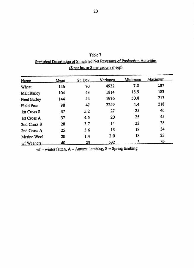
and from the price received for cattle. A statistical description of the net revenues

associated with each enterprise. given the correlations discussed above and given the fann

operator's subjective distributions, is presented in Table 7.

6. Study Results

6.1 Risk-efficient solutions

Assuming that the fann business and financial situation is adequately represented by

the set of resource consttainl'\ imposed in the Target-MOT AD mattix, risk-efficient plans

derived as solutions to the model are described as in Table 8. Each change of basis in the

risk-efficient set is associated with an expected return and a mean negative-deviation from

the target return at that expected rerum. Rb' ·ier production mixes have higher expected

20

Table 7

SYUi~tiQW ~~gjWiQ!l Qf Sinudaled Nel R~vruJY~~ Q{ ProduQtiQ!l A£ti~ti~~ ~ per ba. Qr $ per grown shew

Name Mean St. Dev Variance Minimum Maximum

Wheat 146 70 4932 7.8 :87 Malt Barley 104 43 1814 18.9 183 Feed Barley 144 44 1976 50.8 213 Field Peas 98 47 2249 4.4 218 1st Cross S 37 5.2 27 25 46 1st Cross A 31 4.5 20 25 45 2nd Cross S 28 3.7 11 22 38 2nd Cross A 25 3.6 13 18 34 Merino Wool 20 1.4 2.0 18 23 wfWeaners 40 23 532 3 89

wf = winter fanen, A = Autumn lambing, S = Spring lambing

21

Table 8

Im:~et MOTAD Efficient Sets

Expected Mean Negative Activity Levels

B~tmn~ DevingQO Wh~iU Fbarl~~ Pea~ irS Pa~auml Pil:ilYre2 Labour Qm~r~ Targ~t income level = $107 000

195868 3073 800.0 400.0 200.0 179 9.2 36.8 550.2

193855 2929 768.8 400.0 200.0 243 15.4 61.1 529.3

159853 929 239.5 400.0 200.0 1339 121.3 485.2 173.6

152702 620 128.1 400.0 200.0 1570 143.6 574.3 98.8

150923 558 105.8 400.0 200.0 1616 148.0 592.2 122.2

142489 345 400.0 200.0 1835 169.2 676.8 233.1

Target income level. 125 000

195858 6065 800.0 400.0 200.0 179 9.2 36.8 550:!

187489 5347 669 400.0 200.0 448 35.3 141.0 462.7

166392 3654 341.3 400.0 200.0 1128 100.9 403.8 242.0

153894 2815 146.7 400.0 200.0 1531 139.9 559.4 111.3

15i2702 2763 128.1 400.0 200.0 1570 143.6 574.3 98.8

150269 2678 97.59 400.0 200.0 1633 149.7 598.7 130.8

lS(}211 2677 96.87 400.0 200.0 1634 149.8 599.3 131.6

Target income level = 145 000

195858 8927 800.0 400.0 200.0 178 9.2 36.8 550.2

175313 7310 480.1 400.0 200.0 841 73.2 292.7 335.3

170744 7025 409.0 400.0 200.0 988 87.4 349.6 287.5

167271 6891 354.9 400.0 200.0 1100 98.2 392.8 251.2

162952 6809 287.7 400.0 200.0 1239 111.7 446.6 206.1

22

returns, the number of deviations below the target return also increase to express the

increase in risk. Given the probability-weighted sum of deviations used in this analysis, an

expression of risk is the mean negative~deviation below the target. As listed in Table 8, it is the average negative-<ieviation below target with a one-in-fifty chance of occurring.

By graphing the results of Table 8, Figure 2 is obtained. It shows that allowing

a greater mean negative-deviation below target than 6 065, will not increase revenue above

$195858* when the target revenue is $125000. Similarly, increases in the acceptable

target negative-deviations of 3 073. and 8 927 for the other two target revenues will not

result in revenue increases. Resoun::e constraints and constraints describing production

preferences would have to be broken for net revenue to increast further. On the other

hand, as the level of acceptable deviation below-target is reduced, constraints are

effectively being placed on the optimal production mix. Risk is defined as the mean negative-deviation, and therefore as the level of acceptable deviation is reduced, plans

200000

190000

180000 fI'J

E ti 170000 ex: 11 Tarnet =: 145000

I 160000

150000

140000 0 2000 4000 6000 8000 10000 12000

Mean Negative-Deviation

Figure 2 Risk-Efficient Production Frontiers

23

become less risky and the optimtJ.l expected revenue is reduced. The minimum mean

negative-deviation below target for which any solution can satisfy all consttaints is

indicated by the last entty for each target level in Table 8. Overall, the results show that, as

expected. the fann is forced into a riskier production set as the level of target income is

increased.

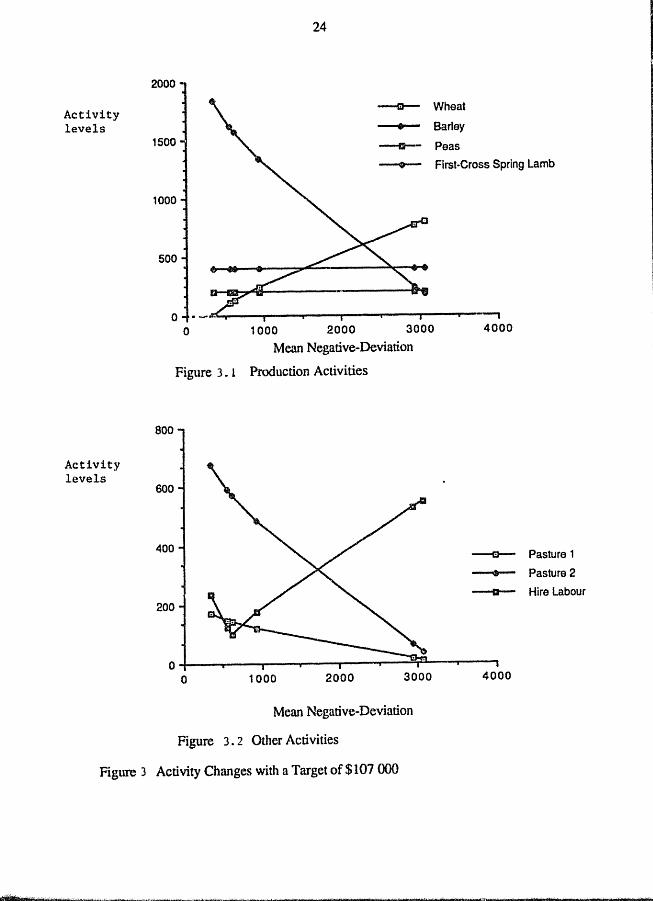
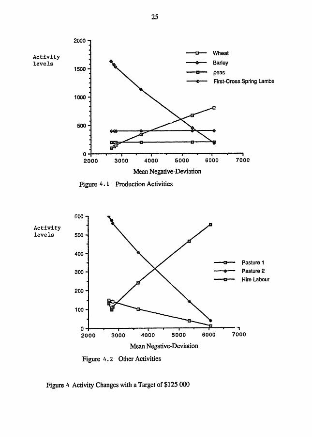
As the expected revenue and acceptable ri.~ is decreased, wheat's place in the

production mix is taken predominantly by first-cross spring lambs. A characteristic decline

in labour, with increases in area of medic pastures is also noticed as a general rule. As a

larger number of ftrst-crass spring-drop lambs is forced into the optimal production mix, to

decrease the mean negative-<ieviation, a requirement for extra labour results in a jump in the

hire labour activity. For ease of recogmtion, the changes in activity levels are drawn across

their critical domains of mean negative-deviation for the three target revenue levels in

Figures 3, 4. and 5.

6.2 Optimal Production Mixes

To maximise expected revenue subject to risk, the production activity mix should be

on the risk-efficient production frontier of the target income under inspection. However,

even if he remains on the frontier) the case-study fanner has a choice of production activity

mixes. Thus, there will be a specific point on the frontier which will define the optimal

production mix. To discover this point one could either elicit a utility function and find the

point of tangency between such a function and the risk-efficient frontier, or one could elicit

the optimal production mix directly from the case-study fanner.

To keep the fann level decision context and to maintain the close involvement of the

case-study farmer, a directly elicited optimal production mix was preferred over one

detennined by a utility function. It was imponant to give the case-study farmer as good an

indication as possible of the distributions of expected revenue from which he could choose.

To provide the farmer with the required understanding of the distributions involved, the

mean-negative deviation is probably not sufficient From an inspection of the output file

for a given target income, the critical infoITuation of the number of years in which revenue

fell below target was recorded, and the range and average of those shortfalls in revenue

could be obtained.

Activity levels

24

Wheat

Barley

Peas

First·Cross Spring Lamb

Activity levels

800

600

400

200

o 1000 2000 3000

Mean Negative-Deviation

Figure 3. 1 Production Activities

4000

-e--

• •

O~--~----~---¥----~--~--~~---T--~ o 1000 2000 3000

Mean Negative-Deviation

Figure 3. 2 Other Activities

Figure 3 Activity Changes with a Targetof$107 000

4000

Pasture 1

Pasture 2

Hire Labour

Activity levels

Activity levels

25

2000

~ Wheat

.. Barley 1500

1'1 peas

• Flrst·Cross Spring lambs

1000

500

O~--~--~--~--~-~~~~~--~--~--~I 2000 3000 4000 5000 aooo 7000

Mean Negative-Deviation

Figure 4. 1 Production Activities

eoo

500

400

300

200

100

~ Pasture 1 .. Pasture 2

-, Hire labour

a ~--~--~--~~~~--~--~--~~~--, 2000 3000 4000 5000

Mean Negative-Deviation

Figure 4. 2 Other Activities

6000 7000

Figure 4 Activity Changes with a Target of $125 000

Activity levels

1400

1200

1000

800

600

400

200

26

--a-- Wheat

~ Barley

111- Peas

• First-Cross Spring Lambs

""--~-----------~~-----e

O~----~----~----~~----?-----~-----6000 7000 8000

Mean Negative-Deviation

Figure 5. 1 Production Activities

600

9000

Activity 500 levels

400

300

200

10:1 i

6000 7000 8000

Mean Negative-Deviation

Figure 5.2 Other Acu.vitip's

Figure 5 Activity Changes with a Target of $145000

-e- Past.Jre 1

• Pasture 2

- Hire labour

9000

27

Table 9 summarises the infonnation presented to the fanner in an interview. The

information from the output fue is for each of the changes of basis which occur along the

risk-efficient frontiers. As well as expected revenue and mean negative-deviation, the

nJ" flber of observations below target and tlleir maximum, minimum and average values

..Jelow target are shown.

Table 9

Summary of B~low Targe! R~venue§

No Expected Mean Negative Number Min Max Average

R~v~n!!~ D~viariQn belQw Im:ge! Devi§don Deviation D~via1ion

Target = $107 000, 30% debt totalling $300 000, interest at 18.75%

1 195868 3073 6 1313 55634 25610

2 193855 2929 5 16910 53708 29291

3 159853 929 4 5120 20337 11 611

4 152701 620 4 855 13319 7744

5 150923 558 3 5880 11 912 9292

6 142489 345 3 2992 8992 5742

Target = $125 000, 35% debt totalling $350 000, interest at 20.75%

7 195858 6065 9 .t. '::16 73674 33696

8 187489 5347 8 13134 65461 33420

9 166392 3654 7 12942 44755 26100

10 153894 2815 7 7179 32490 20105

11 152702 2763 8 1416 31 319 17268

12 150269 2678 8 3743 29394 16736

13 150211 2677 9 38 29349 14870

Target = $145 000, 40% debt totalling $400 000, interest at 22.75%

14 195858 8927 9 9627 93674 49596

15 175: 13 7310 9 7447 735)(\ 40612

16 170744 7025 10 3719 52 1 35126

17 167271 6891 11 4122 65618 31 322

18 162952 6809 12 4254 61 379 28370

28

With the $107 000 target income, the case-study fanner opted for production plan No.1 which \'¥ould maxh"1lise his expected revenue. Under the $125000 target incomep

production plan No.9 was considered optimal. Production plan No.15 was chosen as optimal under the $145000 target income, with a "boom-or-bust" philosophy. Hence, for the two lower levels of debt financing the fanner's selection is in accord with the safety­first criterion of the model. This is evidenced by activities that hav\' lower business risk entering the solution as financial risk is increased. However, at higher levels of debt (and financial risk), a reversal is obseIV~ and a riskier overall solution is selected which contravenes the safety-first criterion. Indeed, later in the interview it become clear that some other components of the model, including crop rotation constraints, would be ignored

by the fanner if debt obligations reached these extreme levels.

7. Summary and Conclusions

Efficient sets of risk management strategies from alternative cropping and livestock activities have been generated as the first objective of this study. While these strategies are efficient, they incorporate the safety-first decision criterion inherent in the target-negative

deviation analysis via the Target-MOTAD technique. This technique allows both financl:al

and business risks to be considered. Financial risks are introduced through the fIXed

financial obligations and the consequent generation of a target income. The study was motivated by the stress on cash flow management from the current business environment, particularly the pressure imposed by the high and volatile interest rates on past 'over­borrowing',

Varying the target has enabled consideration of the second objective of comparing

the effects of various levels of financial obligations on risk-efficlent sets of production

activities. It is evident by the change in optimal production mix of the case-study fanner

between each of the risk-efficient frontiers, that fixed fmancial obligations do affect the optimal production mix of fann enterprises.

As the target income is changed from $107 000 to $125000, business risks are lowered, to compensate for the increase in financial risk, by tht;; choice ,~f a more stable optimal production point, with respect to expected revenue, on tlte risk~tlicient frontier.

29

However, as the target income is increased from $125 000 to $145 000, there is an increase

in business risk as financial risk increases.

8. St&d~ Implications

This study has demonstrated the usefulness of target-negative deviation analysis in

the modelling of decision making in a risky environment An aspect of the study which is considered valuable is the on-farm decision context which was interwoven with the

analysis. The use of generated price and yield infonnation in a cheap, easy-to adjust fashion will allow easy adoption of this process to other fanns. The generated price and

yield observations can be based on the decision maker's most recent experiences and

beliefs, while cost of production estimates based on accounting records further reflected the

fanning practices and financial system of the case-study fann.

While concepts of risk aversion and utility theory are imponant considerations in economic models it is more likely that fanners will be able to relate better to a target return level which they set, and with their own tolerance of returns below the target level when deciding on a management system.

Biological simulation of fann production systems is currently evolving ( White and

Weber 1987; While, Weber, Bowman and McLeod 1989) along with an increasing number

of, and competence in the use of computers. A dynamic, user friendly, personal computer

program which will consider both the financial and business risks, with weightings between predictions of biologically-derived mathematical relationships and the decision maker's own beliefs, taking into account the history of the property, could be developed

with risk-efficient options expressed ill an easily understandable fonn. All infonnation

used in this study is readily accessible to a fann operator with reasonably accurate records;

historical correlations would evolve over time along with the biological yield predictions.

The potential roles of new enterprises in a fann plan could be easily tested by

inclusions of generated prices and yields in the simulated years and by inclqiing

establishment costs in the fixed financial ubligations. Importantly to fann ~urvival. the

Target-MOT AD technique offers a way of modelling the effects of fixed financial obligations in a volatile business environment

30

9 References

ABARE (1988), CommOOit)!.Stati§tics Handbo.:2ka Commonwealth Government Printer, Canben"a.

Anderson, J.R.t Dillon, J.L. and Hamaker, J.B. (1980). Agricultural Decision Analysis...

University of New England Printery, Annidale.

Anderson, l.R. and Lionardi9 A.C. (1982), "A note on the effects of decision criterion and

ponfolio size on the characteristics of efficierit portfolios", Journal of the Acc.Qunting Association QLt.\ysuaUa fwd New Zealand 22(1}, 81-89.

Barry, P.J. (1983),"Financing growth and adjustment of fann finns under risk and

inflation: Implications of micromodeling't t in Saum. K. and Schertz, L. (eds.)

Modeling Faun Decisions for :&lIicy Analysis, Westview Press, Boulder, Colorado.

Bertelsen, D. (1985), "Farm· level risk management: a safety-f:srst analysis", unpublished M.S. thesis, North Dakota State University, Fargo.

Burgess, T and Came, R. (1989), Manager and Commercial Manager of the National

Australia Bank, Annidale. Personal Communication.

Cribb, J. (1989), "Crunch time for primary indusny'\ The Australian June 1, 1989, pl.

Cumming, R.I. (1989) "An investigation of the trade-off between financial risk and

business risk: inferences from a primary producer in the Mallee", unpublished

B.Ag.Bcon. dissenation, Department of Agricultural Economics and Business Management, University of New England, Annidale.

Fishburn, P.C. (l977},"Mean-risk analysis with risk associated with below target

returns," American Economic Reyiew 67(2), 116-126.

Gabriel, S.C.{l979),"Financial responses to changes in busisness risk on central Illinois

grain fanns", unpublished Ph.D. Thesis, illinois University, Urbana.

31

Gabriel, S.C. and Baker,e.B (1980),"Concepts of business and financial plans",

American Journal of Awcultural Economics 62(3), 560-564.

Hall, N.(1988a).Gross Marwns and Farm Machinery Cost for the Victorian Mance 1988.

Technical Report Series No 153, Depanment of Agriculture and Rural Affairs,

Melbourne.

Hallt N. (l988b)l"Stability of dry land fanningtl, The Mallee f~ (newsletter) August 1988, pp.2-3.

Ha7.ell, P.B.R. (1971),"A linear alternative to quadratic and semivariance programming for

fann planning under uncenainty,I1American Journal of Agricultural Economics 53{l),

53-62.

Hooke, G.{l988),"Jnterest rates, the exchange rate and fanners", Review of Marketing and

Agricultural EcQnomi£~ 56(1),91-96.

Markowitz, H. (1952), "Portfolio selection ", Journal of Finan£e 7, 77-91.

Oram, D.A. (1985), The profitability of Alternative Cro.p Rotations in the Wirnmera.

Research Project Series No 205, Victorian Depanment of Agriculture and Rural

Affairs, Melbourne.

O'Sullivan, S.(1987), Qm:mlan. Enterprise Budgets fQr the North West of N.S.W, The

Agricultural Business Research Institute, University of New England, Annidale.

Pederson, 0.0. and BeI1elsen.O. (l986),"Financial risk management alternatives in a whole .. fann settinglt.Western Journal of Agri£uhural EconQmic~ 11(1),67-75.

Porter, R.B. (1974),"Semivariance and stochastic dominance; a comparison", American

Economic Review 64(1),200-204.

Porter, R.B. and Gaumitz, J.E. (1972),"Stochastic dominance vs mean-variance ponfolio

analysis", American Economic Review 62(1),438-446.

32

Powell, R. (1987), Financing Broadacre Agriculture (dmft), Depanment of Agricultural

Economics and Business Management, University of New England.

Pyle, D.H., and Tumovsky, S.l. (1970), "Safety-fust and expected utility maxirlization in

mean-standard deviation ponfolio analysis", Review of EconQmics ar4 Statistics.

52(1), 75-81.

Rickards, P.A. and Passmore, A.L. (l971), "Planning for profit in livestock grazing

systems", University of New En&tand Professional Faun Management Guidebook

N2J., University of New England, Annidale.

Simpson,l. (1989), Berriwillock. Personal Communication.

Tauer, L.G. (1983), 'Target M011AD", AmeriCAn Journal of Agricultural Economics 65(3), 606-610.

Tobin, 1. (1958),ttLiquidity preference as behavior towards risk", Reyiew of Ecooomic

~ 25(1), 65-85.

Tsiang, S.C. (1972), "The rationale of the mean-standard deviation analysis, skewness preference and the demand for money" ,American Economic Review 62(3), 354-71.

(1974), "The rationale of the mean-standard deviation analysis: reply and

errata for original anicle",Aroerlcan Economic Review 64(3),442-50.

U.S.D.A. (1989j), U.S. Wheat Letter Associate§. Washington D.C. May 19, 1989.

U.S.D.A. (l989h), World Grain Situation and Outlook, U.S.D.A. Foreign Agricultural

Service, Grain Series, (FG 4-89.) April 1989.

Watts. M.J." Held. LJ. :.md Helmers, G.A. (1984), "A Comparison of Target MOTAD to

MOTAD", Canadian Journal of Agricultural Economic§ 32(1), 175-185.

Weston, IF. and Brigham, B.F. (1978), Mana~erial Finance, 6th edition, Dryden Press,

Hinsdale, Illinois.

33

White, D.H. and Bowman, P J. (1981), "Dry sheep equivaler j for comparing different

classes of stock," Agnote, Victorian Deparnnent of Agriculture, Melbourne.

White, D.H. and Weber, K .. M. (eds.) (1987). Computer Assisted MBnagement of

Agriculture) Production Systems, Proceedings of a workshop endorsed by Standing

Committee on Agriculture, and held at the Royal Melbourne Institute of Technology

14-15 May, 1987.

White, D.H., \Veber, K.M., Bowman, PJ. and McLeod, c.R. (1989), "The use of

models of sheep and cattle production systems to aid on-fann decision making in

southenl Australia" t Proceedings of the International Gmsslands Congress, Nice,

France.

34

Appendix

Table A.I

~sonal Labour ReQuirements per unit (hours)

A£!ivill Sum~I AYIYmn ~i!U~r S12ring Wheat 1.14 0.47 0.07

Mbarley 0.65 0.33 0.07

Fbarley 0.65 0.33 0.07

Peas 0.70 0.47 0.07

XS 0.20 0.18 0.25 0.54

XA 0.20 0.48 0.25 0.24

XXS 0.20 0.23 0.25 0.49

XXA 0.20 0.49 0.25 0.19

Woolpdn 0.14 0.13 0.19 0.13

Cattle 0.10 0.15 0.15

Pasture 1 0.27 0.47

Pasture2

Sources: Oram (1985).

Hall, N. (1988a).

O·Sullivan (1987).

35

TableA.2

~~ Production (LSM) and Use (PSE)

Season

Activity Summer Autumn Winter Spring

Wheat (2.08)

Mbarley (2.08)

Fbarley (2.08)

Peas (8.32)

XS 1.54 0.90 0.90 1.60

XA 0.90 1.60 1.54 0.90

XXS 2.50 1.30 1.30 2.30

XXA 1.30 2.30 2.50 1.30

Woolpdn 1.00 1.00 1.00 1.00

Cattle 8.30 27.70 10.70

P'dsture 1 (1.00) (1.00) (4.16)

Pasture 2 (2,O8) (4.16) (2.0S) (8!32)

Brackets indicate supply in LSM

Sources: White and Bowman (1981).

Oram (1985).

Xear 1977-78

1978-79

1979-80

1980-81

1981-82

1982-83

1983-84*

1984-85*

1985-86*

1986-87*

1987-88*

Sources: a

36

Table A.3

£rices Returned per tonne

Wh~ta Malting Barley b Fee.d Barley C P~asd 77.57 78.75 71.75

107.35 74.50 67.50

132.72 109.45 101.45 124.68 140.42 132.42

122.19 132.83 127.83

151.38 184.67 184.67

129.72 142.60 125.60**

132.27 123.33 115.30**

127.46 114.85 109.85**

106.75 122.34 97.34** 190.00

124.99 121.45 96.45** 210.00

ABARE (1988).

b Classified as No I-Australian Barley Board Annual Report 1988.

Returns as listed minus costs of the Grain Elevator's Board as supplied by Australian

Barley Board~ Adelaide

C As for 2, except Galleon, a recently introduced variety with Cereal Cist 1'\",

Nematode tolerance taken to have equivalent quality to 'No 3' classified barley-Annual

Report 1988.

d Prices supplied by V.O.P. McrcantilelPersonal comultation.

*

**

Assume participant of Australian Barley Board's 'pool payment

scheme'.

Classification changes to 'No 4' for Gallecm.