an investigation of the relationship between trade
TRANSCRIPT
AN INVESTIGATION OF THE RELATIONSHIP BETWEEN TRADE OPENNESS
AND
ECONOMIC GROWTH IN NAMIBIA
A THESIS SUBMITTED IN PARTIAL FULFILMENT OF THE REQUIREMENTS
FOR THE DEGREE OF
MASTER OF SCIENCE IN ECONOMICS
OF
THE UNIVERSITY OF NAMIBIA
BY
FLORENCE M. SAMUNDENGU
200506251
MARCH 2016
MAIN SUPERVISOR: Dr. J.S. Sheefeni
ii
ABSTRACT
The study investigated the relationship between trade openness and economic growth
for Namibia using annual time series data over the period 1980 to 2011. The variables
used include GDP per capita, labour force, capital formation, trade openness and real
exchange rate. This study employed time series techniques such as unit root, co-
integration, Granger-causality, impulse response function and forecast error variance
decomposition. The Johansen co-integration analysis and Vector Auto-regression
Model (VAR) are used in estimating the long run relationship between trade openness
and economic growth. There was co-integration of variables for trade openness and
economic growth. The results found a positive long run relationship between the
variables. The Granger-causality showed no causation from trade openness and
economic growth. The findings suggest that effective policies that promote labour-
intensive industrial sectors would boost trade for economic growth in Namibia.
Therefore, promoting trade in various avenues can enhance economic growth in
Namibia.
iii
Table of Contents
ABSTRACT .................................................................................................................... ii
ACKNOWLEDGEMENT ........................................................................................... vii
DEDICATION ............................................................................................................. viii
DECLARATION ........................................................................................................... ix
ACRONYMS ................................................................................................................... x
CHAPTER ONE: INTRODUCTION ........................................................................... 2
1.1 Background ............................................................................................................. 2
1.2 Statement of the problem ........................................................................................ 7
1.3 Objective of the study ............................................................................................. 8
1.4 Hypothesis of the study ........................................................................................... 9
1.5 Significance of the Study ........................................................................................ 9
1.6 Limitations of the study .......................................................................................... 9
1.7 Organisation of the study ...................................................................................... 10
CHAPTER TWO: NAMIBIA’S ECONOMIC STRUCTURE AND ITS TRADE
REGIME ....................................................................................................................... 11
2.1 Introduction ........................................................................................................... 11
2.2. Namibia’s economic structure ............................................................................. 11
2.3 Import and export market ..................................................................................... 14
2.4 Investment incentives ........................................................................................... 17
2.4.1 Export Processing Zones ................................................................................ 17
2.4.2 Tax- free regime ............................................................................................. 18
2.4.3 Investment Centre and the Foreign Investments Act ..................................... 19
2.5 Trade regime ......................................................................................................... 20
2.6 Trade policy .......................................................................................................... 24
2.7 Industrial policy .................................................................................................... 25
2.8 Conclusion ............................................................................................................ 28
CHAPTER THREE: LITERATURE REVIEW ........................................................ 30

iv
3.1 Introduction ........................................................................................................... 30
3.2 Theoretical Literature ........................................................................................... 30
3.2.1 The traditional theory ..................................................................................... 31
3.2.2. The new trade theory ..................................................................................... 31
3.2.3 Neoclassical growth models ........................................................................... 33
3.2.4 Endogenous growth theory ............................................................................ 33
3.3 Empirical Literature .............................................................................................. 35
3.4 Conclusion ............................................................................................................ 47
CHAPTER FOUR: METHODOLOGY ..................................................................... 50
4.1 Introduction ........................................................................................................... 50
4.2 Econometric Framework and Model Specification .............................................. 50
4.2.1 Model specification ........................................................................................ 50
4.2.2 Estimation Technique ..................................................................................... 54
4.3 Data, its Measurements and source ....................................................................... 62
4.4 Description of variables ........................................................................................ 63
Definition of variables ............................................................................................. 63
CHAPTER FIVE: EMPIRICAL ANALYSIS AND RESULTS .............................. 69
5.1 Introduction ........................................................................................................... 69
5. 2: Detailed Estimations ........................................................................................... 69
5.2.1 Unit Root Tests .............................................................................................. 69
5.2.2 Co-integration Test ......................................................................................... 73
5.2.3 Vector Error Correction Model ...................................................................... 75
5.2.4 Granger Causality Test ................................................................................... 77
5.2.5 Impulse Response Function ........................................................................... 79
5.2.6 Forecast Error Variance Decomposition ........................................................ 83
CHAPTER SIX: CONCLUSION AND POLICY IMPLICATION ........................ 87
6.1 Conclusion ............................................................................................................ 87
6.2 Discussion of the result and Policy Implication ................................................... 88
6.3 Area for Further Research ..................................................................................... 90

v
References .................................................................................................................. 91
Appendix .................................................................................................................. 102
vi
List of Figures
Figure 2.1. GDP per capital growth rate. ........................................................................ 12
Figure 2.2. Major exporting countries of Namibia ......................................................... 15
Figure 2.3.Trade statistics on import and export in Namibia ......................................... 16
Figure 5.2. Impulse response of output growth .............................................................. 80
List of Tables
Table 4.1 Description of Variables in the Study ............................................................ 63
Table 5.1 Unit root tests: ADF and PP in levels, first and second difference ................ 70
Table 5.2 Unit root test: KPSS in levels and first difference ......................................... 72
Table 5.3 Johansen cointegration test based on Trace and Maximum Eigen Value test of
the Stochastic Matrix ...................................................................................................... 74
Table 5.4 Lag order selection for VAR system .............................................................. 76
Table 5.5 Polynomial stability condition of the VAR system ........................................ 76
Table 5.6 Granger Causality Test results for the generic model .................................... 78
Table 5.7 Variance decomposition ................................................................................. 84

vii
ACKNOWLEDGEMENT
I wish to acknowledge the guidance and support of my supervisors, Dr. J. P. S. Sheefeni
for unwavering support during the course of study. I also wish to acknowledge all the
lecturers in the Department of Economics for being my mentors during my studies and
for excellent contributions, comprehensive comments, suggestions and interesting
discussions which have been important to both the content and structure of this thesis.
Students and classmates are hereby gratefully acknowledged. To my family, especially
Chinemba, my husband, for unlimited support and understanding when not available at
home during my study time, I thank God for being there for me.

viii
DEDICATION
This thesis is dedicated to my lovely family, my husband, Chinemba and my sons,
Kuwunda and Luyando. You are my source of inspiration.
ix
DECLARATION
I, Florence Moono Samundengu, hereby declare that this study is a true reflection of my
own research, and that this work, or part thereof has not been submitted for a degree in
any other institution of higher education.
No part of this thesis/dissertation may be reproduced, stored in any retrieval system, or
transmitted in any form, or by any means (e.g. electronic, mechanical, photocopying,
recording or otherwise) without the prior permission of the author, or The University of
Namibia in that behalf.
I, Florence Moono Samundengu, grant The University of Namibia the right to
reproduce this thesis in whole or in part, in any manner or format, which The University
of Namibia may deem fit, for any person or institution requiring it for study and
research; provided that The University of Namibia shall waive this right if the whole
thesis has been or is being published in a manners satisfactory to the University.
………………………………… Date………………………
Florence Moono Samundengu
x
Acronyms
ACP African, Caribbean and Pacific Countries
ADF Augmented Dickey-Fuller
AGOA African Growth and Opportunity Act
AR Auto-Regressive
ARDL Autoregressive Distributive Lag
BLNS Botswana, Lesotho, Namibia, South African and
Swaziland
BoP Balance of Payments
CET Common External Tariff
CMA Common Monetary Area
CMEA Council for Mutual Economic Assistance
ECM Error Correction Model
ECOWAS Economic Community of West African States
EEC European Economic Community
EFT European Free Trade Association

xi
EPA Economic Partnership Agreement
EPZ- Export Processing Zone
EU- European Union
FDI Foreign Direct Investment
FEVD Forecast Error Variance Decomposition
FMOLS Fully Modified Ordinary Least Squares
FTA Free Trade Agreement
GDP Gross Domestic Product
GIRF Generalized Impulse Response Function
GNP Gross National Product
GRN Republic of Namibia
IMF International Monetary Fund
IV Instrument-Variable
KPSS Kwaiatkowski-Phillips-Schmidt-Shin
LDCs Less-Developed Countries
MERCOSUR Common Market of the South

xii
MFN Most Favored Nation
MTI Ministry of Trade and Industry
NDP National Development Plan
NPT Namibia Press and Tools International
OLS Ordinary Least Squares
PP Phillips-Perron
PPP Purchasing Power Parity
Q1 Quarter 1
Q4 Quarter 4
RISDP Regional Indicative Strategic Development
SAARC South Asian Association for Regional Co-
operation
SACU Southern African Customs Union
SADC Southern African Development
SIPO Strategic Indicative Plan for the Organ
SMEs Small Medium Enterprises

xiii
SPS Sanitary and Phytosanitary
SSA Sub-Saharan Africa
TEs Transitional Economies
TIPEEG Targeted Intervention Program for
Employment and Economic Growth
USA United States of America
USD United States dollars
VAR Vector-Auto Regressive
VAT Value Added Tax
VECM Vector Error Correction Model
WTO World Trade Organization

2
CHAPTER ONE: INTRODUCTION
1.1 Background
The term “trade openness” can be defined as the world’s integration among countries.
According to Osabuohien (2007), openness is likened to a situation where nations of the
world join together so that they have free movement of labor, capital and free trade.
Furthermore, the effect of trade is commended on that it increases competition and
enhances efficiency (Ray, 2012). Trade openness is, therefore, assumed to be an
important source of economic growth and can be measured in two different ways:
activity-based and incentive-focused. According to Shafaeddin (2006) the activity-
based approach considers indicators such as exports plus imports, to gross domestic
product (GDP). The difference with the activity based approach is that trade is
influenced by the export structure and the size of the country rather than trade policy.
Countries exporting mainly primary goods and services, for example, Sub-Saharan
African countries usually depend on trade than countries with a diversified export
structure. The incentive-focused approach relates trade openness to free trade. However,
in developing countries free trade is not possible when it comes to international trade
markets, even when all restrictions are removed. This is because restrictions on trade
through tariffs continue with developed countries. In the case of Namibia, the active-
based approach appears more appropriate.
However, economic growth is defined as an increase in production and consumption of
goods and services in a given year. It is measured by comparing gross national product
3
(GNP) of a given year with the GNP of the previous year. GNP is the value of all goods
and services produced in a country including the value of imported goods and services,
less exported goods and services (Dornbusch, Fischer and Startz, 2004). The principle
of economic growth is assumed to be the improvement in technology, capital stock and
level of literacy. Growth rate is associated with countries joining globalization through
improved openness in international exchange of ideas, technology as well as goods and
services. According to Osabuohien (2007), growth rate is associated with countries
embracing the ongoing globalization and increasing openness to the international
exchange of goods and services as well as ideas and technologies. Krugman (1979)
suggests that gains from international trade are obtained by opening up for trade
between two countries with differentiated products so that more variety is available to
sustain improvement in living conditions in developing countries. The market forces
will channel resources towards relatively productive sectors leading to a rise in
efficiency, hence increasing the total production size of a trading country or increase the
country’s GDP.
It is in view of the above assertions that there is a positive long run relationship between
openness and the rate of growth as suggested by the growth theories, while higher level
of output is obtained through greater openness yield gains to countries mostly in terms
of economic performance according to the static allocative efficiency gains theory
(Eboreine & Iyoko, 2009). Thus, expansion of market size by the domestic exporters as
4
suggested by the new growth theory would result in a higher long run growth rate even
though no positive link was predicted by this theory as increases in openness can
eventually lower growth due to increases in competition. According to Dobre (2008),
there are some important routes to strengthen productivity through openness to trade
such as:
(a) Efficient allocation of resources; trade allows countries to specialise in the
production of goods and services which is cheaper in its raw material/production
or has comparative advantage by exchanging their surplus production with that
of other countries different surplus production.
(b) Economies of scale; without trade, economies of scale are limited by the
domestic market size. Trade allows firms and industries to produce more
efficiently. Trade enhances firms’ innovativeness so that a high producing firm
expands its exports as well as its domestic market. This eventually boosts the
whole economy’s productivity.
(c) Trade can provide access to new technology through goods and services
especially where countries have taken up open trade regime leading to different
stages of the production process that incorporate new technology. Trade also
brings about greater competition which helps reduce monopoly by lowering
prices for consumers and promoting effective competition amongst firms on the
world market.
(d) Investment incentives; incentive for investment through trade can be increased
by creating business opportunities through better access to export and import

5
markets can improve the scope for productive investment thereby increasing
foreign direct investment (FDI). FDI brings about technology and innovation
improvement resulting in more efficient production and enhancing competition
in world market.
Thus, trade openness to economic growth is seen as having a positive outcome. In other
words, trade openness improves integration of human societies through economic
activities around the globe. There is a danger in removing or abolishing quotas
overnight, this may lead to balance of payment adjustment problems. Although,
developing nations mostly rely on trade restriction as a measure to protect domestic
industry and control, their balance of payment eventually distorts their resource
allocation to domestic industry and restrict trade.
There are dynamic effects that are achieved from exposure to imports and exports in
terms of openness. Openness to trade provides structural changes in a given country and
has the potential of reducing poverty to millions of people by allocating domestic
resources in the production for sale or exporting to international markets which has
insufficient domestic demand and can import products that are more expensive to be
produced locally (Salvatore, 2007). Exports can be defined as goods and services
domestically produced for sale to foreign consumers while imports are the buying of
foreign goods and services to be consumed locally (Dornbuch, Fisher and Startz, 2004).
Exports and imports of commercial goods in the past involved strict customs

6
regulations, but nowadays, due to trade agreements between countries, only small
exports and imports are still applicable to legal restrictions. Trade is not only about
export and import, it provides employment opportunities, FDI, which impacts
technological advancement for economic development (Yeboah, Naanwaab, Saleem &
Akuffo, 2012). According to Yeboah et al. (2012), reduction in trade barriers in Europe
has boosted the economic performance due to the creation of a single market.
Trade protection is the major problem despite positive benefit of openness to trade.
Over the last half a century, barriers to trade have dropped although some sectors and
products are still highly protected. Namibia and United States have a trade agreement
which showed that Namibia was 117th largest goods trading partner of the US. Exports
plus imports amounted to $574 million in 2011. The exported goods to the US
amounted to $137 million in 2011, up by 23.6% from 2010 ranked as 142nd largest
goods exporter. In 2011 Namibia was ranked 97th largest importer from the US, which
totaled $436 million, up by 123.6% from 2010 (United States Trade Representative,
n.d.). The balance of trade of a country is improved when the currency is devalued,
which means that volumes of exports increase while a reduction in imports would be
recorded because they have become more expensive. The exchange rate influences how
productive resources are allocated between tradable and non-tradable goods and
services. As such conclusion, the external competitiveness of a nation and position of
balance of payments (BoP) is determined by the exchange rate.
7
The endogenous growth approach found that trade policy has an impact on both the
level of income and the long-run rate of growth of an economy through scale,
allocation, spillover, and redundancy effects. On the other hand neither the opening up
of trade nor different patterns specialisation can affect the rate of growth, but are
determined only by comparative advantage in the neoclassical approach (Matadeen,
Matadeen & Seetanah, 2011). Some studies concluded that openness played an effective
role in developed countries, whereas many studies also concluded openness can play a
significant role in developing countries.
In 2010 Namibia’s gross domestic product (GDP) was US$ 12.2 billion. GDP per capita
income was measured using purchasing power parity (PPP) was US$ 6,323. The Gini
Co-efficient was 0.63 (UNDP, 2011). With regards to trade openness and economic
growth in Namibia, it appears little has been done in the area of relating trade openness
and economic growth studies. It is against this background that the proposed study
would like to narrow the gap in the available literature of trade openness and economic
growth and recommend policy actions which may be considered by the Ministry of
Trade and Industry (MTI).
1.2 Statement of the problem
A number of studies have been done on trade openness and economic growth over the
years in developing countries (Rodriguez, 2006, Osabuohien, 2007, Sarkar, 2007 and
8
Ahmadi and Mohebbi, 2012). In the case of Namibia, Eita and Jordan (2007) and
Nashiidi and Ogbokor (2013) investigated only the export-led growth in Namibia.
Unlike other previous studies, this study goes further to investigate the question of how
strong the correlation between openness and economic growth is and whether
international trade is able to ensure improvement in the living conditions of its citizens.
The latest Labour Force Survey (2012) indicated that unemployment rate was at 27.4%.
Through the Industrial Policy statement, the government of Namibia introduced a
programme called Targeted Intervention Program for Employment and Economic
Growth (TIPEEG) in order to fight unemployment by increasing total factor production,
improve trade and enhance the competitiveness of the economy (Ministry of Industry,
2012). The findings of this study seek to provide a better understanding of the
relationship between openness and economic growth.
1.3 Objective of the study
The broad objective is to examine the relationship between trade openness and
economic growth in Namibia.
The specific objective is to examine the causal relationship between trade
openness and economic growth.
Based on the derived results, policy recommendations will be made.

9
1.4 Hypothesis of the study
The research hypotheses to be tested are listed as follows:
H0: There is no relationship between trade openness and economic growth in Namibia.
H1: There is relationship between trade openness and economic growth in Namibia.
1.5 Significance of the Study
The study is expected to highlight the importance of trade openness and economic
growth in Namibia and areas in which policymakers can improve in order to enhance
economic growth in Namibia. The study will also benefit other organisations (local and
international) looking for areas of investment which would have a high likelihood of
increasing the country’s GDP and so addressing economic problems such as
unemployment and poverty.
1.6 Limitations of the Study
The research will utilise secondary data. As such methodological limitations of omitted
variable bias are foreseen such as stake holders’ views on international trade and
economic growth will not be collected. The other limitation is the time factor, that is,
the time given to complete the research poses a challenge.
10
1.7 Organisation of the Study
The study is organised as follows: Chapter 2 focuses on Namibia’s economic structure.
Chapter 3 analyses the literature review both theoretical and empirical literature.
Chapter 4 covers the methodology used in the study. Chapter 5 reveals the empirical
results. Lastly, chapter 6 provides conclusions and recommendations.

11
CHAPTER TWO
NAMIBIA’S ECONOMIC STRUCTURE AND ITS TRADE REGIME
2.1 Introduction
The purpose of this chapter is to provide an overview of Namibia’s trade and economic
structure. The chapter is organized as follows: section 2.2 reviews Namibia’s economic
structure, section 2.3 reviews the import and export market and section 2.4 reviews
investment incentives. Section 2.5 reviews its trade regime, Section 2.6 reviews the
trade policies and Section 2.7 reviews the industrial policies, whilst Section 2.8
concludes the chapter.
2.2. Namibia’s economic structure
The World Bank and the IMF classified Namibia as a middle-income developing
country. According to the Namibia Statistics Agency (2012), Namibia has an estimated
household population of 2 066 398 and a Gini- coefficient of 0,597. It is still among
nations with the highest income inequality, with economic growth of 4.5% in 2011
compared to 4.6% in 2012 (BoN, 2012).
On the monetary side, the Namibian currency is pegged at the same rate with the
neighbouring South Africa’s currency, an economy 40 times larger (Sherborne, 2009).
This means that policy makers in South Africa determine important economic variables
such as prices, interest rates and exchange rates. In addition, Namibia is a resource-

12
based economy because primary industries contribute more to GDP than secondary
industries. The primary industries comprise agriculture, fishing and mining. Global
growth was estimated at 3.9% in 2011 and eased to 3.2% in 2012.
Figure 2.1. GDP per capital growth rate. Reprinted from National Planning
Commission-Central Bureau of Statistics (2013).
Figure 2.1 above shows GDP per capita growth from 1980 to 2012 using data obtained
from the World Bank. The World Bank (2013) states that Namibia has experienced a
steady GDP growth, moderate inflation, limited public debt and steady export earnings
despite a GDP growth decline in 2009. In 2009 GDP growth declined by 1% due to the
decline in external demand for minerals. The GDP measures the national income and
output for a given economy of a country and is equal to the total expenditures of all
final goods and services produced at a given period of time within the country. It is
accepted that countries with good export performance also do well in their Gross
Domestic Product (GDP) performance and vice versa (Jordaan & Eita, 2007).
0
20,000
40,000
60,000
80,000
100,000
120,000
19
80
19
82
19
84
19
86
19
88
19
90
19
92
19
94
19
96
19
98
20
00
20
02
20
04
20
06
20
08
20
10
20
12
VA
LUE
(N$
)
YEARS
GDP per capita
13
Historically, Namibia’s GDP from 1980 to 2011 averaged 4.3 billion USD reaching a
high of 12.3 billion USD in December of 2011 and slowed down in December of 1985
with 1.4 billion USD due to a global crisis. Namibia’s GDP value represents 0.02% of
the world economy (World Bank, 2012).
The prudent management of fisheries resources has led to significant contributions to
GDP and to foreign exchange earnings of the fishing sector. A decade before
independence (1980-1989), there was rampant illegal fishing and overfishing in
Namibia’s Zone of the Atlantic Ocean (Odada & Matundu, 2008). At independence in
1990 the government of the Republic of Namibia (GRN) had to deal with the fishing
industry by finding ways of restoring a totally depleted fish stock, by establishing a
Ministry of Fisheries and Marine Resources, which introduced fishing quotas to allocate
fish catch to Namibian fishing companies so as to minimize the over-fishing problem.
The fishing sector then increased significantly with an annual contribution of foreign
exchange earnings of 18.2%, while the mining industry contributes 37.6% to foreign
exchange earnings and service sector contributes 19.8% (Odada and Matundu, 2008).
The global economic crisis of 2008/09 demonstrated the vulnerability of the Namibian
economy to external shocks that led to the slowdown of Namibia’s mining sector and
hence economic construction of 2009. Overall, inflation rate has been of single digit
except in 2002 and 2008. Inflation rate hit 11.3% in 2002 due to depreciation of the
South African Rand to which Namibian Dollar is pegged, causing higher importation of
inflation while the 2008 rate was attributed to fuel and food prices global spike. By

14
2011 the inflation rate slowed down to 5% and increased to 6.5% in 2012 due to rising
inflation on food and transport (BoN, 2012).
When it comes to trade and structure of trade in Namibia, according to Bank of
Namibia’s annual report (2012), the economic slowdown in advanced economies
adversely affects growth in developing economies because of reduction in their export
external demands.
2.3 Import and export market
The Namibian economy is not well diversified as it is concentrated in primary sector
activities namely the extraction and processing of minerals, commercial livestock
farming and fishing. This makes Namibia vulnerable to short and long-term
environmental shocks (World Bank, 2013). According to trade information obtained
from the Trading Economic (2013), Namibia imports are concentrated on machinery
which include electrical equipment, vehicles, transport equipment, petroleum products
and fuel, chemicals, metals and food beverages. The top traditional trade partner is
South Africa. This is because of the close historical links between the two nations.
Namibia’s imports that come from neighboring South Africa, the major import partner,
represents 66% of Namibia’s imports. South Africa is followed by the Netherlands,
United Kingdom and China.
When it comes to exports, Namibia’s main export is diamond (25% of total exports).
Other exports include uranium, lead, zinc, tungsten, tin, fish, tourism, livestock, logistic
15
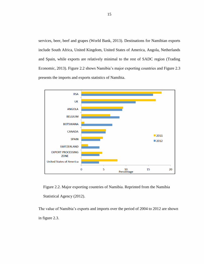
services, beer, beef and grapes (World Bank, 2013). Destinations for Namibian exports
include South Africa, United Kingdom, United States of America, Angola, Netherlands
and Spain, while exports are relatively minimal to the rest of SADC region (Trading
Economic, 2013). Figure 2.2 shows Namibia’s major exporting countries and Figure 2.3
presents the imports and exports statistics of Namibia.
Figure 2.2. Major exporting countries of Namibia. Reprinted from the Namibia
Statistical Agency (2012).
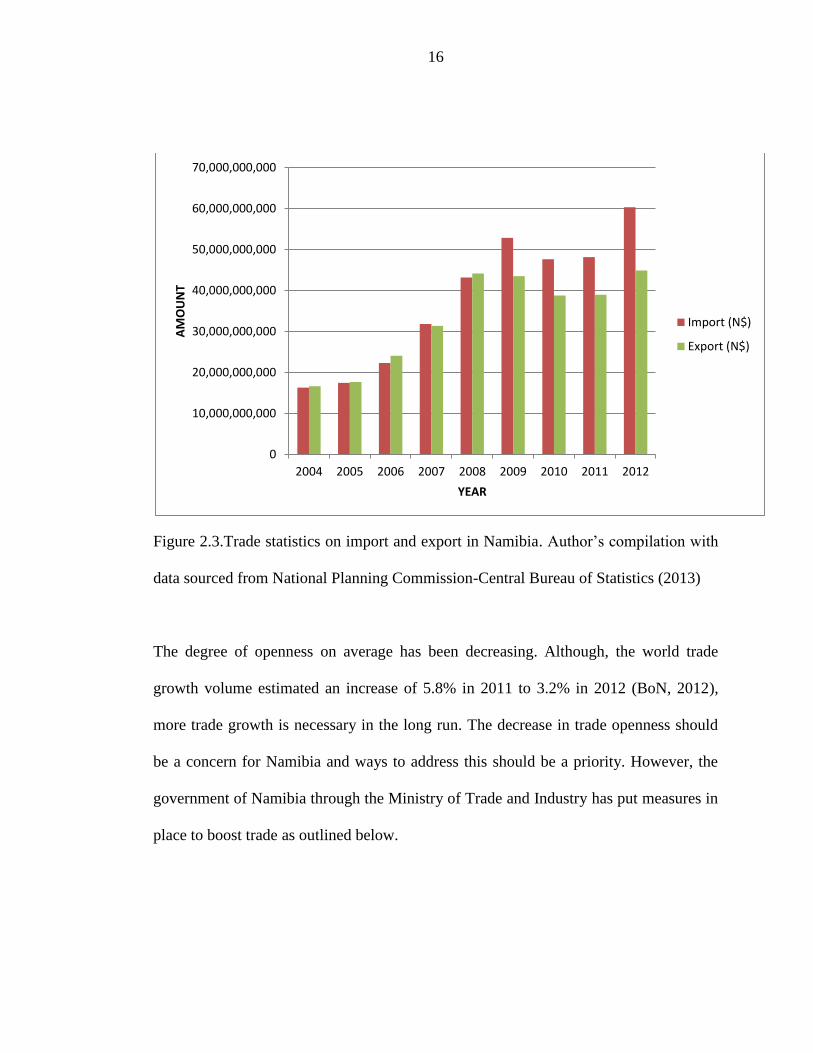
The value of Namibia’s exports and imports over the period of 2004 to 2012 are shown
in figure 2.3.
16
Figure 2.3.Trade statistics on import and export in Namibia. Author’s compilation with
data sourced from National Planning Commission-Central Bureau of Statistics (2013)
The degree of openness on average has been decreasing. Although, the world trade
growth volume estimated an increase of 5.8% in 2011 to 3.2% in 2012 (BoN, 2012),
more trade growth is necessary in the long run. The decrease in trade openness should
be a concern for Namibia and ways to address this should be a priority. However, the
government of Namibia through the Ministry of Trade and Industry has put measures in
place to boost trade as outlined below.
0
10,000,000,000
20,000,000,000
30,000,000,000
40,000,000,000
50,000,000,000
60,000,000,000
70,000,000,000
2004 2005 2006 2007 2008 2009 2010 2011 2012
AM
OU
NT
YEAR
Import (N$)
Export (N$)
17
2.4 Investment incentives
The Ministry of Trade and Industry adopted investment incentives to boost export and
growth through value addition. Investment incentives are offered in Namibia and many
other developing countries to attract FDI inflows. First, are the fiscal incentives which
are policies that are designed to reduce tax burden of a firm (Banga, 2003). Fiscal
incentives include tax concessions in the form of reduction of the standard corporate
income tax rate, accelerated depreciation allowances on capital taxes, exemption from
import duties on capital taxes, exemption from import duties and duty drawbacks on
exports. Fiscal incentives do affect location decisions especially for export oriented
FDI. Second, are the financial incentives, which involve direct contributions to the firm
from the government (including direct capital subsidies or subsidised loans).
2.4.1 Export Processing Zones
The government of Namibia adopted the export processing zones (EPZs) in 1995 to
mainly boost export and ultimately economic diversification. As a policy instrument
(GRN, 2006). The main objectives of EPZs are to:
Facilitate imports of raw materials and capital
Facilitate the transfer of technical and industrial skills to the local labor
force
Contribute towards an increased share of the manufacturing sector to job
creation and GDP
18
Enhance the diversification of the local economy
Namibia’s EPZ regime offers export oriented manufacturers a range of internationally
competitive advantages. Currently, the EPZ has attracted a number of local and
international interests. Some 20 companies are fully operational benefiting from the
EPZ incentives. These companies are from Africa, Asia, Europe and North America
(http:/www.wbepzmc.iway.na). The companies established under EPZ in Walvis Bay
produce products such as automotive parts for vehicles such as VW and Audi,
assembling of vehicles, clothing, diamond cutting and polishing, fishing accessories and
plastic pallets and products. The major companies under EPZ are: Roach Investments,
Marine Ropes International, Transvecho and Namibia Press & Tools International
(NPT). The city of Walvis Bay is located strategically to reduce costs on transportation
where bulk cargo is efficiently handled.
2.4.2 Tax- free regime
EPZ enterprises are exempted from corporate income tax, duties and value added tax
(VAT) on machinery, equipment and raw materials imported into the country for
manufacturing purposes. The only taxes paid are the income tax on employee’s income
as well as the 10% withholding tax (non-resident shareholders) on declared dividends.
The local and international investors who meet the conditions for admission under the
EPZ enjoy equal treatment and eligibility to the EPZ incentives.
19
2.4.3 Investment Centre and the Foreign Investments Act
The Namibian Investment Centre was established in 1992. It falls under the Ministry of
Trade and Industry and serves to assist the minister in the administration of the Foreign
Investments Act (GRN, 1993). The act allows foreign nationals to invest and engage in
any business activity in Namibia, which any Namibian may undertake provided they
comply with any formalities or requirements prescribed by any law in relation to the
relevant business activity.
It is, therefore, important to have knowledge of factors which influence investment for
economic planning and macroeconomic forecasting purposes. The Income Tax Act
makes the following provision for incentives on manufacturing activities and the export
of manufacturing goods only such as:
125% deduction of cost of remuneration and training of employees
involved in manufacturing
125% deduction of export expenditure on goods manufactured in
Namibia
125% deduction of land- based transportation costs of material and
equipment to be used in a manufacturing activity
Taxable income derived from manufacturing is taxed at 18% only for a
period of 10 years
20
The deduction of the erection costs of a building of 20% in the first year
and 8% per annum for the next 10 years
80% exemption of taxable income derived from the export of
manufactured goods (excluding fish and meat).
2.5 Trade regime
Namibia is a member to regional and multilateral trade arrangements and economic
groupings such as: the Southern African Customs Union (SACU), Southern African
Development Community (SADC), African, Caribbean and Pacific (ACP) Countries,
World Trade Organization (WTO), SACU-European Free Trade Area (Iceland,
Liechtenstein, Norway and Switzerland) Trade Agreement, SACU-MERCOSUR
(Argentina, Brazil, Chile, Paraguay and Uruguay) Trade Agreement and SACU-India
preferential Trade Agreement. Namibia’s trade and industry policies are primarily
formulated and implemented by the Ministry of Trade and Industry. They are also set
and influenced at regional and multilateral level of its membership. Some of the
mentioned organizations are briefly discussed below.
SACU is one of the oldest and successful unions dating back to 1910. Re-negotiations
were signed in 1969 between newly independent countries of Botswana, Lesotho and
Swaziland with South African. Namibia became a member after its independence in
1990 with special focus on barriers to trade, customs and trade facilitation, trade and

21
investment promotion and sanitary and phytosanitary (SPS). The main objectives of
SACU includes: SACU members significantly benefit from revenues that come through
customs and excise duties which are pooled in the common revenue pool and then
divided among member states of Botswana, Lesotho, Namibia, South African and
Swaziland (BLNS). The revenue share is determined by the country’s economic
performance. SACU member states prescribe a common external tariff (CET) on
imports from non- SACU members. It also allows free movements and transit of goods
without any tariff within the customs union.
SACU revenue is the major contributor to Namibia’s budget, for example, in 2007 there
was an increase in payment from SACU which put Namibia’s budget into a surplus
since its independence. SACU income to Namibia dropped in 2010 and 2011 due to
global recession with a total revenue averaging 39.3% of total average. In 2011/2012
Namibia’s total revenue and grants from SACU was estimated at N$26,9 billion,
decreased than originally estimated at N$28,0 billion (SACU, 2012), while in
2010/2011 the revenue outturn was estimated at N$22,7 billion. This decrease in
revenue was as a result of a decline in SACU revenue (SACU, 2010/11).
There are some limitations also for BLNS states in how they engage in SACU
agreements such as:

22
Difficulty for BLNS countries to protect their infant industry against South
Africa.
Difficulty to influence new investment in industries for BLNS states due to
South Africa’s dominance.
Countries such as Namibia, Lesotho and Swaziland who are members of the
Common Monetary Area (CMA) agreement lose monetary policy powers.
As a step towards improving its international market access, Namibia is also a member
of SADC which was transformed from the Southern African Development Coordination
Conference (SADCC) in 1992. The aim of SADC is to improve trade and security
within the region. The SADC Trade Protocol was signed in Maseru, Lesotho in August
1996 and came into effect in 2000. A Free Trade Area was established among member
states and amended the rules of origin in August 2008. Furthermore, according to
SADC Summit Report 2005, SADC had set goals by 2010 to have a customs union, and
monetary union with one single regional currency by 2015. The member states
comprise of Angola, Botswana, Democratic Republic of Congo, Lesotho, Malawi,
Mauritius, Mozambique, Namibia, Seychelles, South Africa, Swaziland, Tanzania,
Zambia and Zimbabwe.
SADC’s major project is expansion of the political and economic integration, under the
policy document entitled ‘Regional Indicative Strategic Development Plan (RISDP)’. It
involves markets integration and prevention of poverty of member states. The other is
23
the Strategic Indicative Plan for the Organ (SIPO), which deals with the security policy.
According to Odada and Matundu (2008) there are a number of shortcomings in SADC,
the biggest being the lack of political will and inconsistency to agree on a common
strategy. There is inadequate economic diversification, low capacity and human skills
and weak enforcement power within the member states, mainly due to conflicts of
interest since some SACU members are also members of SADC. In addition, the
regional court (SADC Tribunal) was formed with the aim of resolving conflicts and
disputes between and among member states. However, because of complications in the
SADC’s organisational structure, the SADC Tribunal hardly acts. In short, for regional
integration process to be strengthened, deficiencies in the SADC region need to be
fixed.
Namibia is still negotiating for an Economic Partnership Agreement (EPA) between
SADC-EPA group and the European Union (EU). Under the Cotonou Agreement,
Namibia enjoys the “interim” agreement with the EU and other four SADC-EPA group
members. Namibia continues negotiating as part of the SADC-EPA group for a
comprehensive EPA with the EU. Under the African Growth and Opportunity Act
(AGOA), Namibia still benefits from duty free and quota-free entry of some particular
goods into the United States. Furthermore, SACU and members of the European Free
Trade Association (EFTA) signed a free trade agreement (FTA) in May 2008. This
improved Namibia’s market access for SADC countries export’s to have free entry into
24
the EFTA countries, while tariffs on imports from the EFTA countries continue to fall
or will eventually be abolished. Only industrial goods, processed agriculture products
and fish are covered in this FTA. SADC signed another preferential Trade Agreement
(PTA) in April 2009 with the Common Market of the South (MERCOSUR). According
to World Bank (2010), Namibia was ranked 66th out of 183 countries in 2009 ease to do
business with and 31st out of 39 in Sub-Saharan Africa (SSA) region.
This shows that Namibia depends on imports and exports from the global market with
the primary products being the major exports mostly to South Africa and the EU. The
country’s total exports of goods and services as a percentage of GDP in 2011 was
47.4% compared to 44.7% in 2010. While, imports of goods and services as a
percentage of GDP slumped to 52.4% in 2011 compared to 54.7% in 2010 (World
Bank, 2013).
2.6 Trade policy
Namibia has no formal trade policy according to the World Bank Indicators (2010). Its
tariff policy is governed by the Common External Tariff (CET) of the Southern African
Customs Union (SACU). When it comes to trade regime, Namibia is more open
compared to an average sub-Saharan African (SSA) country by 11.3 percent. The
highest level of tariff protection of 12.6% is given to the agriculture sector and non
agriculture sector is 9.6%. Measurement of the country’s trade policy’s pace is the
25
wedge between bound and applied tariffs which is currently at 11.4%. Namibia’s
average MFN applied tariff has remained consistently steady over the past few years at
7.8%.
Due to Namibia’s participation in various trade forums; regionally and internationally,
the country is guided by the following trade policy notions:
To create and maintain just and mutually beneficial relations among nations.
To identify the need and respond to globalization as a powerful trend and world-
wide economic liberalization.
To improve the country’s economic diversification drive through viability of
domestic production and trading in goods and services.
To create regional co-operation and integration through joint trade negotiations
with more powerful economic blocks such as the WTO, the European Union and
the USA.
Another policy which outlines the principles and parameters towards industrialization of
the state is a policy statement document called the Industrial policy.
2.7 Industrial policy
The Industrial policy involves the short, medium and long term goals and action plans
by the government of Namibia’s approach and strategies on industrialization. The
policy document aims at improving stakeholder’s policies and programs in line with
government plans towards achieving Vision 2030. The government believes that the

26
domestic private sector is the engine for job creation and economic growth. It will,
therefore, support the private sector wherever possible in achieving higher production,
increasing exports, reduce unemployment rate and income distribution disparities
through achieving a competitive real effective exchange rate. In this regard, to reduce
the escalating unemployment rate which was recorded at 51% by the latest labour force
survey undertaken in 2012, a new program was introduced by the government called
Targeted Intervention Program for Employment and Economic Growth (TIPEEG) in
helping fight unemployment, as a long-run job creation measure, which will result in
total factor production, hence competitiveness of the economy. Furthermore, the
industrial policy stipulates the following:
Limited resources- Due to limited resources, the industrial policy will
follow the targeted approach at any point in time. Identified sectors with
specified needs during a particular period in time will be supported with
clear documentation highlighting such priority. Such an approach will be
the integrated development approach, which will be built on market
integration, industrial development and infrastructure development.
As a small country sized population, of about 2 million, the economic
policy will focus on openness towards market access in products and
services domestically produced through regional economic integration,
which is a WTO key element towards economic openness.
27
Namibia’s development and manufacturing practices will be emphasised
on going green. Currently, the gas emission levels are low and protection
of future industrialisation plans is of great benefit to Namibia and the
global market.
Incentives- The incentive regime aims at implementing measures for
industrial competence and capacity development resulting in increased
production possibility frontier, which will also make it easier to set up
business and operate effectively in Namibia. Furthermore, other
incentive regimes include the export development programmes, and
support schemes such as economic zones, special-purpose vehicles and
the tax regime.
Political stability- This includes other institutional factors such as the
property rights and rule of law. The strategy is to observe closely what
emerging economies are doing and adapt to future trends, making
investors see Namibia differently from other developing African
countries.
Development and promotion of SMEs- some important issues to be
looked at by the Namibian Government include the following;
The SME entrepreneurs’ development programs and training
promotion
Advocating for banking conditions/regulations easier for SME
bank to set up business Namibia

28
2.8 Conclusion
This chapter looked at the Namibian economic structure and its trade regime. Namibia
is classified as a middle-income developing country by the World Bank and the IMF.
Although, Namibia has achieved moderate economic growth over the past few years, it
is still among nations with the highest income inequality. Namibia is a resource-based
economy with a growing primary sector. Namibia’s export market is concentrated on
extraction and processing of minerals, commercial farming and fishing. These products
are exported mainly to South Africa and to Europe. Furthermore, Namibia’s imports
comprising largely machinery, petroleum products and food and beverages come
mainly from South Africa. Namibia’s growth performance from the 1980s has been
slow compared to other developing nations. The constraints to growth could be related
to factors such as high levels of inequality in income and wealth and the monetary
integration with South Africa, which is a diversified economy and causes a huge impact
to domestic industry.
In trying to avoid the Namibia from being vulnerable to short and long-term
environmental shocks, the government has formulated a number of programmes and
policies aimed at promoting domestic and foreign investment to improve economic
growth in order to achieve the structured goals. Some of these include the Industrial
policy, the Fourth National Development Plan (NDP 4) and Vision 2030.
29
Namibia is a member of regional and international organisations that influence its trade
activity. At the regional level, Namibia is a member of SACU and SADC.
Consequently, Namibia’s fiscal contribution to national budget, its trade policies and
other bilateral agreements are influenced by its membership. At the international level,
the European market is important to Namibia because of export access which is duty
free on meat and fish products, therefore, the EU markets play a major role by
contributing to SACU revenue pool.
The world is increasingly becoming integrated as a global village and Namibia should
continue to diversify its economy, because in the long-run only diversified and
competitive domestic industries will survive competition from multinational industries.
Economic theories show that countries that trade more tend to grow faster. Openness to
trade allows efficient allocation of resources to effective productivity, providing access
to new innovation and technologies. This leads to long-run sustainable growth rate of
the economy. Despite major trade agreements in allowing free trade among member
states, protectionism on trade continues to slow down our economies out of poverty.

30
CHAPTER THREE
LITERATURE REVIEW
3.1 Introduction
This chapter provides an overview of theoretical and empirical literature in order to
understand how trade openness affects economic growth. The chapter is organised as
follows: - Section 3.2 reviews theoretical literature on trade and growth. A review of
recent empirical literature will be presented in Section 3.3 and Section 3.4 core growth
model and Section 3.5 conclude the chapter.
3.2 Theoretical Literature
The theoretical link between trade and growth is provided in brief exposition. It is
argued that the effect of openness on steady-state growth in theoretical analysis is
ambiguous (Obadan & Okojie, 2010).
Following the theoretical contributions by Romer (1990) and empirical work of Levine
and Renelt (1992), the core growth model explanatory variables included are:
investment, population growth, initial human capital and initial per capital. However,
Greenaway et al (2002) also added to this list of explanatory variables, terms of trade
variables and trade liberalization proxies. In this regard, this work is in tandem with the

31
views of Greenaway et al (2002). There are a number of trade theories applicable to
openness and economic growth such as, the traditional theory, dynamic theory, new
trade theory, and growth theory. They are discussed below.
3.2.1 The traditional theory
The traditional theory, assumes free trade through imports and exports are the best
strategies from the welfare point of view. These welfare improvements are due to
specialised gains according to the comparative advantage in which a country that opens
up can be assured of trade benefits in a static model and consumption gains are
explained in the Ricardian model where a country specialises in producing goods in
which it has comparative advantage. On the other hand, the Hecksher- Ohlin-
Samuelson model shows gains in the two country model, two factor models in which
each country specialises based on their factor endowment. Obadan and Okojie (2010)
assert that international trade is only possible if perfect competition is allowed to prevail
and other things held constant. Imperfect competition may include externalities and
absent of uncertainty in both countries. In the traditional theory, growth originates from
trade (Obadan & Okajie, 2010).
3.2.2. The new trade theory
Furthermore, the new trade theory assumes imperfect competition. The new trade
theory is associated with Krugman (1986) among others. The assumption of perfect
competition and non existence of externalities are important in the traditional theory,
32
but are relaxed in the new trade theory. Under conditions of imperfect competition the
new trade theory concludes that trade restrictions to trade could be welfare gain
(Obadan & Okajie, 2010). However, Matadeen, Matadeen and Seetanah, (2011) argue
that the theory is based on trade policy rather than between trade volumes and growth.
According to Webster (2003), in international arena trade, restrictions are used to win
market power, which can get rid of foreign competitors. For instance, products can be
sold below marginal cost or underpriced until the competitors leave the market; this is
known as predatory pricing. When this happens, producers with market power can then
switch to mark-up pricing. At international level, having market power allows or makes
it possible to increase output and market share. This eventually allows production at a
decreasing average cost in industries characterised by economies of scale and smaller
foreign competitors stand no chance to produce under such conditions.
In the externality case, spillovers in the production process between social marginal
costs and private costs can also be welfare improving. Relevant externalities are linked
to the following: first, is the physical capital accumulation; second, is the accumulation
of human capital or improvement in human skills (such as job on training and education
of workers) and third, is the introduction of new technology. Firms of an economy can
benefit from one another if positive externalities exist amongst each other. These results

33
continue to be argued between trade-growth links (Yanikkaya, 2003). The last theory is
the growth theory which includes both the neoclassical and endogenous growth
theories.
3.2.3 Neoclassical growth models
The neoclassical theory is associated with Ramsey (1928), Solow (1956) and Koopmans
(1965). The neoclassical model assumed closed economy, but analyses of open
economies in recent years apply this growth model. The neoclassical model centers its
works in international economics, macroeconomics and public finance in which it uses
a wide range of aggregate economic analysis (Obadan & Okajie, 2010). Solow model
introduced a number of related facts to economic growth in which the system adjusts to
a given growth rate of labour force and steadily reaches a steady state of proportional
expansion, such as the relative constancy of capital-output ratio over time. The model
states that trade has a positive impact on the level of income (Matadeen et al., 2011).
3.2.4 Endogenous growth theory
Endogenous growth theory can be defined as economic growth form within a system,
mostly a state or a country. This growth theory was pioneered by Grossman and
Helpman (1991) Romer (1990) and Lucas (1988). Obadan and Okajie (2010) state that
the difference between this model and the other theories stated before, is that per capital
output growth converges to zero in the steady state resulting in a positive correlation
between investment rates and growth across countries. To the newly industrialised
34
countries, this theory provides hope due to the different ways of development without
relying on trade alone. It focuses on education and new technology development for the
world market. According to Stensnes (2006), the model thereby explains its long-run
increases in output growth rate; it has the following five phenomena.
Firstly, trade liberalisation may promote economic growth by accelerating the rate of
technological change. Secondly, export-oriented development strategy leads to higher
growth due to some strictly economic factors. Thirdly, there is export of technology
from industrialised countries to developing countries through foreign direct investment
(FDI). Fourthly, external capital for development through outward orientation is
possible. Lastly, an open economy improves its rate of economic growth through
economies of scale in production and through positive spillover effects from
technological development. However, Romer (1990) outlined the four basic
preconditions for growth which are: investment, population growth, initial human
capital and initial per capital.
The model explains how countries can develop within the global market by finding
complementary goods and services (like education) within their economic and political
boundaries. It is, however, difficult to theoretically address the strengths, relevance and

35
validity of each factor in relation to trade and economic growth. Each should be
determined by empirical studies.
3.3 Empirical Literature
The empirical literature on openness and growth is indeed extensive. A number of
studies relate the difficulty in measuring openness. In determining the relationship
between trade openness and economic growth and the direction of causality, a range of
research has been undertaken both country specific and cross country. While some
studies confirmed a positive impact of openness on growth, others did not. In this
section, the empirical literature discussed covers the link between trade openness and
income, export growth and economic growth, the causal link between trade openness
and economic growth, the relationship between trade openness and economic growth
and the indirect impact of openness and economic growth.
The impact of trade on income has no strong presumption on theoretical literature, but
same empirical literature has examined the link (Irwin and Tervio, 2000, Dollar and
Kraay, 2002 and Rodrik and Rigobon, 2004). Irwin and Tervio (2000) assessed the
impact of trade on income during the twentieth century with time period from pre-world
war 1 of 1913 to post war 1990, using cross country regression with sample of 62 and
40 countries. The ordinary least squares (OLS) estimation and the two-stage least
squares (2SLS) estimation methods were used. The results showed a positive impact of
trade on income.
36
Dollar and Kraay (2002) investigated the link between trade and income, using a large
sample of 92 developed and developing countries selected from East Asia and Pacific,
Latin America, Sub-Saharan Africa, Middle East, North Africa, West Africa, Canada,
United States, Latin America and Caribbean over a period of four decades using OLS
methods. The results showed that in middle-income countries like Korea, poor people
are better off than those in India as average income in Korea is higher than in India. The
study concludes that openness to international trade improves income of the poor by
increasing overall incomes, although the findings confirm the need for further research
in income distribution changes. The author further recommended that openness to
international trade and fiscal policies should be the focal point of effective strategy to
poverty reduction.
Rodrik and Rigobon (2004) estimated the interrelationships between openness,
democracy, rule of law and income using the method of identification through
heteroskedasticity (IH). The dataset of 86 countries split into two sub-samples of
colonies versus non-colonies and continents of East-west (Eurasian countries) versus
those of North-South axis (Africa and the Americas) with time period of the twentieth
century. The results showed that openness has a negative impact on income levels, but
has a positive effect on the rule of law. While both democracy and rule of law improve
economic growth.
37
Harrison (1996) estimated the link between trade and poverty in 51 countries using
cross country regression with time period 1960 to 1984. Results showed no evidence of
positive relationship between openness and economic growth. The study concluded that
the poor never benefits from globalization due to unequal distributions from trade.
Another strand of literature on export growth and economic growth is essentially a
dynamic one and, therefore, can be studied in a dynamic framework based on time
series data. Some studies done include Ekanayake (1999), Vohra (2001) and Din
(2004). A study done by Ekanayake (1999) used annual time series data from 1960 to
1997 to examine the causal relation between export growth and economic growth in
developing Asian countries. A co-integration and error-correction model technique was
used. The results showed a bi-directional causality in seven of the eight countries, with
short-run Granger causality running from economic growth to export growth. It was
concluded that there was little evidence of causal relation between export growth and
economic growth.
Vohra (2001) examined the role of export-growth in five Asian countries namely India,
Pakistan, Philippines, Malaysia and Thailand using time series data from 1973 to 1993.
The empirical results show that exports have a positive and significant impact on
economic growth on countries that have obtained a level of economic development.
India and Pakistan were exceptions. The results also confirm that export expansion
strategies and promotion of foreign investment are important for liberal market policies.

38
Din (2004) examined annual time-series data for the export-led growth hypothesis for
the five largest economies of the South Asian region, namely Bangladesh, India, Nepal,
Pakistan, and Sri Lanka using a multivariate Vector-Auto Regressive (VAR)
framework, the concept of Granger causality was employed to determine the direction
of causation between export and output. For India and Sri Lanka, the sample period is
from 1960 to 2002, whereas for Nepal it is 1965 to 2002. For Bangladesh and Pakistan,
the sample period is from 1973 to 2002. The results showed a bi-directional causality
between exports and output growth in the short-run for Bangladesh, India, and Sri
Lanka. There was long-run relationship for Bangladesh and Pakistan among exports,
imports, and output, whereas, no evidence of a long-run relationship among the relevant
variables was found for India, Nepal, and Sri Lanka.
In another study analysing the causal linkages between openness and growth are
outlined. In the issue of causality, economic growth is Granger-cause openness. This
means supporting the growth driven trade hypothesis for a given country (Iyoko and
Eboreime, 2009, Matadeen et al, 2011 and Bajwa and Siddiqi, 2011). The study by
Iyoko and Eboreime (2009) used time-series data from 1981 to 2006, the co-integration
techniques investigated the causal relationship between globalisation and economic
growth in Nigeria. Variables used were globalisation proxied by openness and foreign
direct investment (FDI). This was built on the Mendel Fleming’s model of open
macroeconomics. The results showed a unidirectional causality between FDI and
growth with FDI Granger causing growth and no causality between openness and
39
growth. However, openness Granger caused external debt in Nigeria. The study
concluded that appropriate strategies for development such as effective exchange rate
policy, domestic fiscal discipline diversification of the domestic base and debt reduction
should be encouraged for implementation in Nigeria.
Matadeen et al. (2011), used time-series data using bi-annual data for the period 1989-
2009, through a Vector Error Correction Model (VECM) to investigate the causal links
between trade liberalisation and economic growth of Mauritius. They found that
openness enhances growth and also trade openness indirectly promotes economic
growth by boosting private physical capital in the short-run. A study by Bajwa and
Siddiqi (2011) investigated the casual link between trade openness and economic
growth for four South Asian countries, that is, Bangladesh, India, Pakistan and Sri-
Lanka using Panel cointegration and fully modified ordinary least squares (FMOLS)
technique for periods 1972 to 1985 and 1986 to 2007. The motive was to determine
what happened before and after the implementation of South Asian Association for
Regional Co-operation (SAARC). The results showed that from 1972 to 1985 there
existed a short-run unidirectional causality and from 1986 to 2007 a short-run bi-
directional causation existed. Finally, a positive long-run causality existed between the
variables.
40
It was noted that South Asian countries should implement export oriented policies and
export value added products which will require technological advancement, for rapid
economic growth will be expected in the region.
There is a study with empirical evidence of indirect impact of openness to economic
growth through investment and productivity. The use of openness to growth is highly
sensitive due to the fact that endogeneity which prevents the correct estimation of link
between trade and growth is not controlled. Most of cross sectional studies revealed an
indirect impact For instance, the influential study by Levine and Renelt (1992) assessed
the impact of trade on income in 92 countries for the past four decades during the
twentieth century using cross-country regression. Results found indirect impact between
economic growth through investment and productivity.
There are a number of studies which argue that trade does not impact economic growth.
The authors included Vamvakidis (2002) and Hassan and Islam (2005).The study by
Vamvakidis (2002) examined the relationship between trade openness and economic
growth in developed and developing nations using a cross country regression for the
time period data from 1920 to 1990. The results showed that before 1970 there was no
positive relationship between openness to trade and economic growth. In 1930s the
correlation obtained was negative. The study concluded that only recent phenomena
have shown a positive relationship between trade openness and economic growth. The
findings further indicate that trade was only linked to growth only after the 1970s, not
41
before. Thus, the study confirms that national policy must be linked to trade policy to
improve the economic growth.
Hassan and Islam (2005) investigated the role of financial development and openness
on economic growth in Bangladesh using time series data from 1974 to 2003. Johansen
co-integration test and Granger causality test was done. Results showed that there was
no co-integration relationship and no causal relationship detected in Granger causality
test between financial development and growth and trade openness and growth.
Although a bi-directional causal link was found between financial development and
trade openness. However, the study concluded that financial development can mutually
contribute to poverty reduction.
Adhikary (2011) examined the linkage between trade openness, capital formation, FDI
and economic growth in Bangladesh. The study used annual time series data period
from 1986 to 2008 and employed Johansen-Juselius procedure and vector error
correction model. Results found a negative, but diminishing influence of trade openness
on GDP growth rates.
The impact of openness on growth is highly sensitive to the measure of openness used.
Most analysts face the problem of measuring trade liberalization. Empirical studies have
not been clear on this issue. Where some studies found positive link, others found no
link or negative link due to different proxies and methodology for liberalization, hence
42
questioning the measure of openness and the robustness of variables (Levine and
Renelt, 1992). In their study of trade liberalization and its impact on growth,
Greenaway, Falvey and Foster (2001) employed the panel data technique and random-
effects model. The reason for their study is to argue there is inconclusive evidence of
previous work. In their study, the measure of openness developed was based on
deviations of actual trade from the expected, given factor endowments and geographical
characteristics of the country. The additional literature to this study includes the use of
panel framework to examine inter-temporal and inter country variation. The panel
model provided a dynamic interpretation of the link between trade and growth. The
results found a positive and significant relationship between trade and growth
suggesting a measure of openness is quite robust. In this regard, the study recommends
that government should promote level of infrastructure thereby boosting imports by
reducing domestic transport costs.
However, there are also studies that examined the relationship between trade openness
and economic growth. Such studies confirmed a positive link while a few did find a
negative impact to growth depending on the technique applied. Some influential
contributions include the following Sarkar (2007), Osabuohien (2007), Capolupo and
Celi (2008), Kim (2008), Obadan and Okojie (2010), Marelli and Signorelli (2011),
Yeboah, Naanwaab and Saleem (2012), Ahmadi and Mohebbi (2012). Sarkar (2007)
examined the relationship between openness (trade-GDP ratio) and economic growth of
51 countries, with 16 rich countries and 35 less-developed countries (LDCs) using a

43
cross-country study of averages and panel regression analysis data from 1981 to 2002.
Results showed that only 11 rich and highly trade dependent countries have higher real
growth which is associated with higher trade share. A study of individual less-
developed country experience was also done using time-series Autoregressive
Distributive Lag (ARDL) approach with time period 1961 to 2002. The results showed
that the majority of less-developed countries experienced no positive long-term
relationship between openness and growth. The study concluded that only the middle
income groups experienced a positive long-term relationship.
Capolupo and Celi (2008), used panel estimators for comparing three different groups
of countries namely; the historical European Economic Community (EEC), the
countries of former Council for Mutual Economic Assistance (CMEA) customs union
and a group of Transitional Economies (TEs) with data set from 1960 to 1990 to
examine whether trade openness spurs economic growth. The results showed that the
coefficient of real openness for the two groups which are EEC and CMEA had a
negative sign, but TEs group had a positive sign meaning that there is no robust and
positive relationship between trade and growth. Transition countries benefit more in
terms of productivity growth through trade from international transfer than western
counterparts. Thus, the study concluded that there should be an indirect connection that
goes from trade to investment and then growth.
44
Osabuohien (2007) examined the impact of trade openness on economic performance
focusing on Ghana and Nigeria (ECOWAS members) using time series data from 1975
to 2004 employed vector Autoregressive (VAR) Approach. They found a unique long-
run relationship between economic performance, trade openness, real government
expenditure, labour force and real capital stock. The results showed that openness to
trade was to benefit Ghana more than Nigeria
Kim (2008) used the instrument-variable (IV) threshold regressions approach of time
period 1960 to 1995 for 61 countries to investigate whether the effects of trade openness
may differ along with the level of economic development. Results showed differences
of trade effects on long run economic growth. This confirmed that developed countries
have a greater trade openness resulting to more beneficial effects on long-run growth
and standard of living, while less developed countries experienced a significantly
negative influence to growth and real income through international trade. There long
and short of it is that developed countries should undertake more outward-oriented
reforms, for sustainable economic growth and development while developing countries
should undertake more conservative trade policies.
Obadan and Okojie (2010) used annual time-series data covering the period 1980 to
2007 to examine the effects of trade on economic growth and development in Nigeria.
Variables used included growth rate of GDP, openness, exchange rate, foreign direct
investment, domestic investment and political stability. The results showed that trade

45
openness had a positive impact on economic growth in Nigeria and a strong negative
impact on growth due to political instability. It was concluded that Nigeria’s export base
which solely depend on petroleum should be diversified to include agricultural and solid
minerals export.
Marelli and Signorelli (2011) used panel data model from 1980 to 2007 with an
instrumental variable approach for two countries namely; China and India by focusing
on trade dynamics, degree of openness, FDI flows and specialization patterns and also
estimate the links between openness and growth, for the two countries in terms of their
integration in the global economy. Results showed that both countries in the short-run
had high degree of openness despite being hit by big economic shocks like the 2008-09
global crisis, but concluded that there was a positive and statistically significant growth
effects of opening up and integrating in the world economy. The robust growth of the
two “giant” nationals is currently helping the entire world economy recovery because
they experienced a small deceleration in their growth paths during the first global
impact of the crisis.
A study by Yeboah, Naanwaab and Saleem (2012), used alternative panel models from
1980 to 2008 to examine the relationship between trade and productivity. The Cobb-
Douglas production function estimated the impact of FDI, exchange rate, capital-labour
ratio and trade openness on GDP for 38 African countries. The results showed that 17
countries growth was above average while majority countries were below average

46
returns-to-scale. This confirmed a positive relationship between trade openness and
GDP.
A study by Ahmadi and Mohebbi (2012) examined the effect of trade openness on
economic growth in Iran using OLS method for estimation parameters from 1971 to
2008. Results indicated significant positive effect of trade openness on economic
growth in Iran and concluded that oil revenue and investment growths have a significant
positive effect on economic growth in Iran.
In the case of Namibia Ogbokor (2005) examined on the macro-economic impart of
trade on the Namibian growth using bivariate and multivariate models from 1991 to
2001on time series data. Variables used included exports, foreign direct investment
(FDI) and GDP .The study focused more on exports and inward foreign direct
investment as a source of growth, without including imports. Results showed that FDI
and exports are important for the growth of the Namibian economy. The study
suggested an aggressive export industrialized policy.
Jordaan and Eita (2007) estimated annual time-series data for the period 1970 to 2005
using the error correction model (ECM) to analyse the causality between exports and
GDP. Results showed that exports Granger cause GDP and GDP per capita. It was
concluded that export incentive promotion has a positive influence on growth in GDP.

47
Kalumbu and Sheefeni (2014) examined factors leading to changes in terms of trade
and how the terms of trade impact economic growth in Namibia. The study employed
time series for the period 1980 to 2012 using Vector auto regression technique.
Variables used included real GDP and net barter terms of trade (NBTT). The results
showed a uni-causal relationship from economic growth to terms of trade and a negative
relationship between terms of trade and economic growth in Namibia. Table 3.1in the
appendix shows different approaches used to identify openness and shows how in some
instances, this may have resulted in different findings.
This research will be based on the growth theory because this theory competently
addresses questions of trade and economic growth. Due to the difficulty in measuring
openness, a number of studies have used different measures to examine the effects of
trade openness on economic growth.
3.4 Conclusion
The chapter reviewed a number of growth theories. The endogenous growth theory has
been used as the basis of the study because it is concerned with economic growth from
within a system or a country. The theory competently addresses questions of trade and
economic growth. Due to successes of outward-looking countries emerging and inward-
looking countries failing, trade openness was widely seen to favour economic growth
such as improving the size of market, economies benefit from specialization, and
48
increases its returns to scale. Further trade openness allows government to adopt
policies that are less distortionary and macroeconomic management types that are more
inclined towards international level of competitiveness as part of their growth strategies.
The empirical literature reviewed above, showed that the methodology and variables
used play a role in the results that emerge from the studies. Most of the studies used
time-series data and employed Vector Auto regression (VAR) approach while others
employed Error Correction Model. The other method mostly used is the panel
technique, where the overall results showed a positive link between openness and
economic growth despite different methodologies and openness proxies used. In some
cases Granger causality ran uni-directional and in some cases it ran bi-directional from
trade openness to economic growth. Furthermore, the instrument-variable (IV)
technique was used by Kim (2008), results showed a negative influence of trade
openness to growth in some countries. In addition, Ahmadi and Mohebbi (2012) used
OLS method with results showing a positive relationship between trade openness and
economic growth. However, a robust and clear relationship is yet to be established
between openness and economic growth.
From the theoretical literature most studies support the positive relationship between
trade and economic growth.

49
However, there are still econometric weaknesses such as variables used, omitted
variable bias and different methods of trade openness. In the case of Namibia, Eita and
Jordan (2007) and Nashiidi and Ogbokor (2013) investigated only the export-led growth
in Namibia. Jordaan and Eita (2007), estimated time-series data for the period 1970 to
2005 using the error correction model (ECM) to analyse the causality between exports
and GDP in Namibia, whereas Nashiidi and Ogbokor (2013) investigated export-
economic growth in Namibia, using annual time series data over the period 1970 to
2008 using the Johansen co-integration technique and VECM for the Granger causality
test. The next section provides the methodological path of the study.
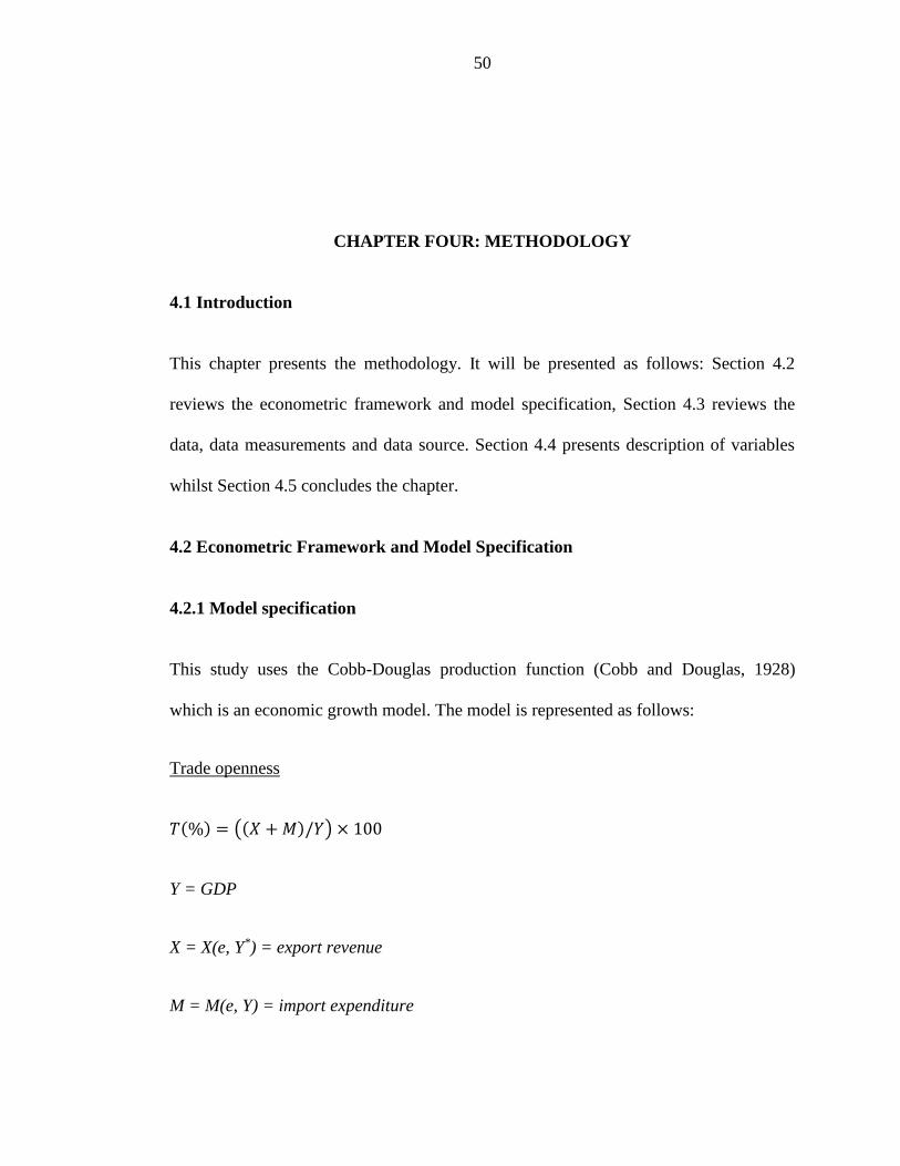
50
CHAPTER FOUR: METHODOLOGY
4.1 Introduction
This chapter presents the methodology. It will be presented as follows: Section 4.2
reviews the econometric framework and model specification, Section 4.3 reviews the
data, data measurements and data source. Section 4.4 presents description of variables
whilst Section 4.5 concludes the chapter.
4.2 Econometric Framework and Model Specification
4.2.1 Model specification
This study uses the Cobb-Douglas production function (Cobb and Douglas, 1928)
which is an economic growth model. The model is represented as follows:
Trade openness
𝑇(%) = ((𝑋 + 𝑀)/𝑌) × 100
Y = GDP
X = X(e, Y*) = export revenue
M = M(e, Y) = import expenditure

51
=> T= f(e, Y, Y*)
Inverse the above function to get Y function
=> Y = f(T, e, Y*)
e: exchange rate,
Y*: foreign GDP
Assume Y* is constant, Y = f(T, e)
For per capita measure, y = f(T, e) (1)
Neo-classical economic growth theory
y = f(k) = AK α (2)
y: per capita GDP
k: per capita capital
Combine (1) and (2) getting
y = f(T, e, k,) (3)
Equation (4) is augmented by including additional factors thereby output becomes a
function of trade openness, exchange rate, capital stock and labour.
y = f(T, e, k,)=Y = AK α Lβ e (4)

52
Where:
Y is per capita GDP is used to capture the level of economic performance, K and L are
capital and labour inputs respectively, while parameters α and β are their shares of
output Y. A is production, trade openness will be proxied by exports + imports / GDP,
L is labour force which will be proxied by population growth and K is real capital stock
which will be used as gross fixed capital formation. According to Osabuohien (2007),
real exchange rate is another additional factor following Yeboah et al (2012). An
implicit form of equation (3) is shown below:
GDPt = f (RKt Lt TROPt RERt) (5)
Furthermore, in explicit form equation (2) can be expressed as follows
𝐺𝐷𝑃𝑡 = 𝐴𝑡 𝑅𝐾𝑡𝛿1 𝐿𝑡
𝛿2 𝑇𝑅𝑂𝑃𝑡𝛿3 𝑅𝐸𝑅𝑡
𝛿4 𝑢𝑡 (6)
Where:
GDP : Real per capita gross domestic products
RK : Real capital stock (proxied by gross fixed capital formation)
L : Labour force in the economy (proxied by population growth)
TROP : Degree of trade openness for the country
RER : Real exchange rate

53
u : Stochastic term used to capture other variables in the model not included.
Time dimension is represented by subscripts‘t’. The linear form of equation (5) above
can be done by taking logarithm of both sides of the equation as follows:
𝑙𝑜𝑔 𝑝𝑔𝑑𝑝 = 𝛿0 + 𝛿1 𝑙𝑜𝑔 𝑟𝑘 + 𝛿2 𝑙𝑜𝑔 𝑙 + 𝛿3 𝑙𝑜𝑔 𝑡𝑟𝑜𝑝 + 𝛿4 𝑙𝑜𝑔 𝑟𝑒𝑟 + 𝑒 (7)
Where:
δ0 is log A, the intercept of the regression equation
e is log U which denotes the log of residuals and
δi′s (i=1,…, 5) are parameters to be estimated that measures the rate of change in the
dependent variable.
Specifying the production in log-liner form (with an error term) the model may be
written as:
𝑝𝑔𝑑𝑝 = 𝛼 + 𝛽1 + 𝛽2 + 𝛽3 + 𝛽4 + 𝛽5 + 𝑢 (8)
The apriori expectations are that δi′s> 0.

54
4.2.2 Estimation Technique
Test for Stationarity
In econometric analysis the stationarity of variables is very important when studying the
different time series behavioral patterns. There are three conditions to be satisfied for
series to be stationary as shown below:
the constant mean through time, thus
𝐸(𝑋𝑡) = 𝜇 (9)
the constant variance through time, thus
𝑉𝑎𝑟(𝑋𝑡) = 𝐸[(𝑋𝑡 − 𝜇)] = 𝜎2 (10)
the covariance which relay upon the number of periods between two values, thus
𝐶𝑜𝑣(𝑋𝑡 , 𝑋𝑡+𝑘) = 𝐸[(𝑋𝑡 − 𝜇)(𝑋𝑡+𝑘 − 𝜇)] = 𝑌𝑘 (11)
As shown above, according to Gujarati (2003) variables that are non stationary could lead
to spurious regression results. Furthermore, non stationary variables could lead to incorrect
conclusion thereby leading to incorrect policy formation. The problem of non stationarity
can be prevented by differencing the variables several times to obtain stationarity.
This approach examines the patterns and trends in the data. It also tests for the order of
integration of the time series variables so as to obtain a meaningful regression analysis
against spurious. This will be achieved by testing for stationarity (unit root). There are
several methods used such as the Augmented Dickey-Fuller (ADF) test (Dickey &
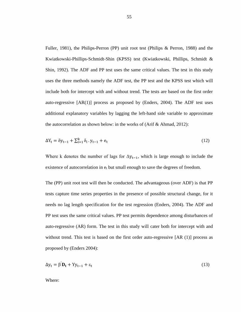
55
Fuller, 1981), the Philips-Perron (PP) unit root test (Philips & Perron, 1988) and the
Kwiatkowski-Phillips-Schmidt-Shin (KPSS) test (Kwiatkowski, Phillips, Schmidt &
Shin, 1992). The ADF and PP test uses the same critical values. The test in this study
uses the three methods namely the ADF test, the PP test and the KPSS test which will
include both for intercept with and without trend. The tests are based on the first order
auto-regressive [AR(1)] process as proposed by (Enders, 2004). The ADF test uses
additional explanatory variables by lagging the left-hand side variable to approximate
the autocorrelation as shown below: in the works of (Arif & Ahmad, 2012):
∆Yt = δyt−1 + ∑ δiki=1 . yt−1 + et (12)
Where k denotes the number of lags for Δyt−1, which is large enough to include the
existence of autocorrelation in et but small enough to save the degrees of freedom.
The (PP) unit root test will then be conducted. The advantageous (over ADF) is that PP
tests capture time series properties in the presence of possible structural change, for it
needs no lag length specification for the test regression (Enders, 2004). The ADF and
PP test uses the same critical values. PP test permits dependence among disturbances of
auto-regressive (AR) form. The test in this study will cater both for intercept with and
without trend. This test is based on the first order auto-regressive [AR (1)] process as
proposed by (Enders 2004):
∆yt = β′𝐃𝐭 + Yyt−1 + εt (13)
Where:
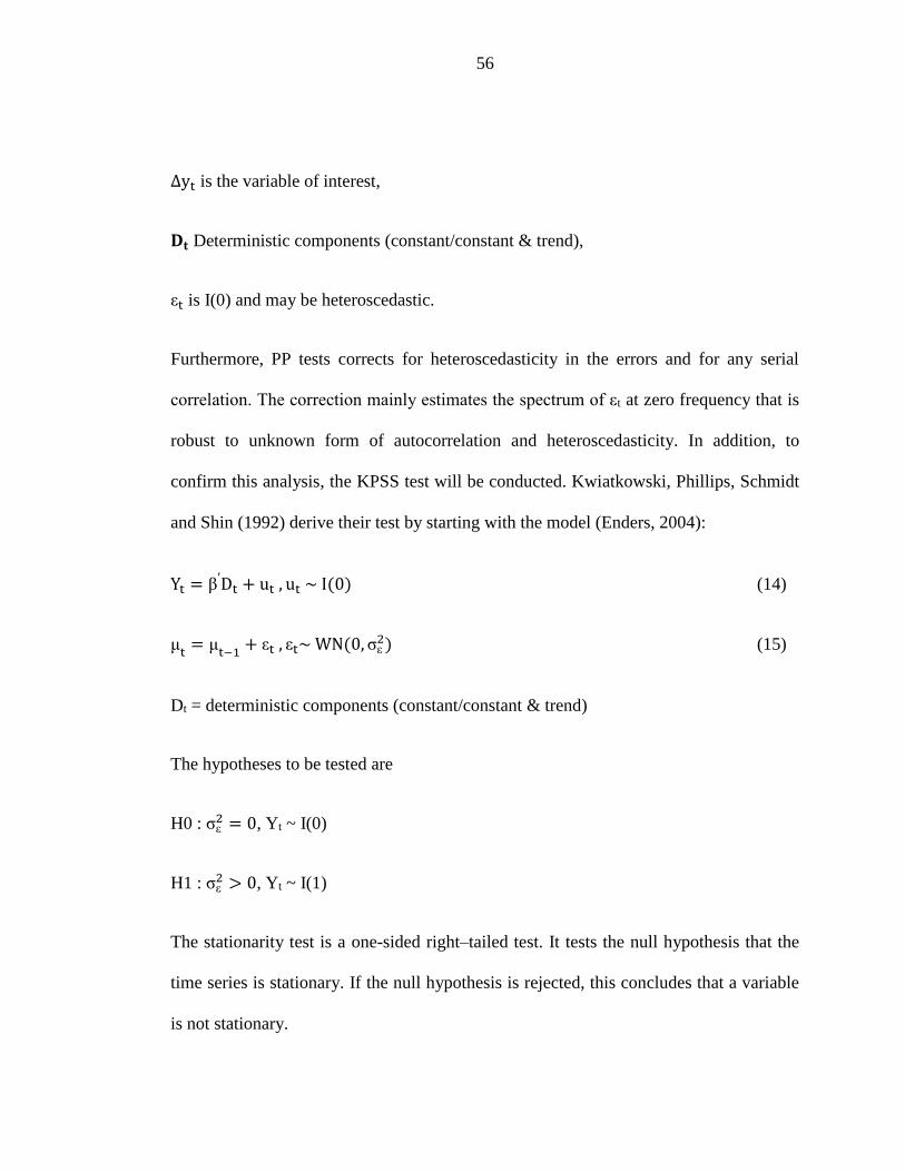
56
∆yt is the variable of interest,
𝐃𝐭 Deterministic components (constant/constant & trend),
εt is I(0) and may be heteroscedastic.
Furthermore, PP tests corrects for heteroscedasticity in the errors and for any serial
correlation. The correction mainly estimates the spectrum of εt at zero frequency that is
robust to unknown form of autocorrelation and heteroscedasticity. In addition, to
confirm this analysis, the KPSS test will be conducted. Kwiatkowski, Phillips, Schmidt
and Shin (1992) derive their test by starting with the model (Enders, 2004):
Yt = β′Dt + ut , ut ~ I(0) (14)
μt
= μt−1
+ εt , εt~ WN(0, σε2) (15)
Dt = deterministic components (constant/constant & trend)
The hypotheses to be tested are
H0 : σε2 = 0, Yt ~ I(0)
H1 : σε2 > 0, Yt ~ I(1)
The stationarity test is a one-sided right–tailed test. It tests the null hypothesis that the
time series is stationary. If the null hypothesis is rejected, this concludes that a variable
is not stationary.
57
Testing for Co-integration
Co-integration means a long run relationship of variables linked at equilibrium when
individual series are non stationary in levels, but after differencing become stationary. If
long run properties are comparable of two or more series then they are known to have
co-integrated. It is possible that individual series could diverge and be unstable in the
short run from each other, but in the long run equilibrium values may converge. The
importance of co-integration helps in identifying the short run and long run
relationships and also prevents non stationary series from the problem of spurious
regression.
As stated earlier, co-integration eliminates spurious regressions of non stationary series.
After the order of integration is tested and should the variables be found to be integrated
of order one or I (1), then tests for co-integration between variables can be conducted.
There are two approaches commonly used in co-integration testing, the Engle and
Granger (1987) and the Johansen (1988) likelihood ratio test. The study will follow the
latter test since the Johansen procedure is correct for endogeneity and autocorrelation.
This procedure allows for co-integration of multiple equations unlike the Engle and
Granger which allows for one co-integrating equation. This means that in Engle and
Granger errors obtained in the first step are carried on to the second step. AS such
testing for co-integration using the Johansen procedure the generalized VAR model is
shown below as follows:

58
zt = A1zt-1 + A2zt-2 +…Apzt-p + εt (16)
Where:
zt is all the n variables in the VAR
A1,…,Ap and B are matrix of coefficient to be estimated
εt is the error term.
The two VAR models will be estimated as follows;
Δyt = βy0 + βy1 Δyt-1 +…+ βyp Δyt-p + y1 Δxt-1 + + yp Δxt-p - y(yt-1-α0- α1 xt-1) + 𝜈𝑡𝑦
(17)
Δxt = βx0 + βx1 Δyt-1 +…+ βxp Δyt-p + x1 Δxt-1 + + xp Δxt-p - x(yt-1- α0- α1 xt-1) + 𝜈𝑡𝑥
(18)
Where:
yt = α0 + α1 x1 is the long-run co-integrating relationship between the two variables and
y and x are parameters, they measure how y and x react to deviations from long-run
equilibrium. When it comes to decision making using the t-statistics, the rejection of the
null hypothesis means that, the calculated value of the test statistics is greater than the
critical value, meaning the null hypothesis of no co-integration is rejected. In that case it
can be concluded that that there is co-integration. Co-integration has two statistic
processes as given below: in the works of (Sheefeni, 2013):
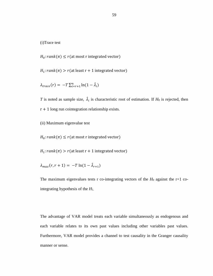
59
(i)Trace test
𝐻0: 𝑟𝑎𝑛𝑘(𝜋) ≤ 𝑟(at most r integrated vector)
𝐻1: 𝑟𝑎𝑛𝑘(𝜋) > 𝑟(at least r + 1 integrated vector)
𝜆𝑡𝑟𝑎𝑐𝑒(𝑟) = −𝑇 ∑ ln(1 − �̂�𝑖)𝑛𝑖=𝑟+1
T is noted as sample size, �̂�𝑖 is characteristic root of estimation. If H0 is rejected, then
r + 1 long run cointegration relationship exists.
(ii) Maximum eigenvalue test
𝐻0: 𝑟𝑎𝑛𝑘(𝜋) ≤ 𝑟(at most r integrated vector)
𝐻1: 𝑟𝑎𝑛𝑘(𝜋) > 𝑟(at least r + 1 integrated vector)
𝜆𝑚𝑎𝑥(𝑟, 𝑟 + 1) = −𝑇 ln(1 − �̂�𝑟+1)
The maximum eigenvalues tests r co-integrating vectors of the H0 against the r+1 co-
integrating hypothesis of the H1.
The advantage of VAR model treats each variable simultaneously as endogenous and
each variable relates to its own past values including other variables past values.
Furthermore, VAR model provides a channel to test causality in the Granger causality
manner or sense.

60
Granger causality test
Granger causality in this study will use VAR model. Granger causality is used to give
direction of possible causality between pairs of variables this is due to Granger (1986).
A simple Granger causality test involves two variables x and y. The equation is shown
as follows:
𝑥𝑡 = ∑ 𝛼𝑗𝑝𝑗=1 𝑥𝑡=𝑗 + ∑ 𝛽𝑗
𝑝𝑗=1 𝑦𝑡=𝑗 + 𝑢𝑡 (19)
𝑦𝑡 = ∑ 𝜂𝑗𝑝𝑗=1 𝑥𝑡=𝑗 + ∑ 𝑦𝑗
𝑝𝑗=1 𝑦𝑡=𝑗 + 𝑣𝑡 (20)
The null hypotheses to be tested are:
H1: 𝜂𝑗= 0, j = 1 …p which means that the x does not Granger cause y; and
H1: 𝛽𝑗= 0, j = 1 …p which means that y does not Granger cause x
For example if x aids in the prediction of y, if it’s true, then x is said to “Granger cause”
y. If none of the hypothesis is rejected, this means that x do not Granger cause y and y
also does not Granger cause x. This shows that the two variables are independent of
each other. Granger causality helps in forecasting ability, but does not give true
causality. If causality lacks from both sides of the two variables, this means that the two
variables are interdependent. The importance of the direction of causation helps in
economic policy strategies. For instance, if causation runs from trade openness to GDP
growth then trade openness promotion strategies should be implemented as an
61
appropriate method for economic growth for a country. On the other hand, if causation
runs from GDP growth to trade openness then the country is expected to increase in its
trading, thereby focusing on its economic growth policies.
Apart from estimating Granger causality, the VAR Mode can also be used to examine
the impulse response function and the variance decomposition.
Impulse Response Function
The impulse response function traces effects of shocks on all the endogenous variables
in dynamic marginal effects on their current and future values. This allows the
establishment of duration the effects of shocks takes to die out (Enders, 2004).
A simple bivariate VAR (1)
𝐼𝑃𝑡 = 𝑎11𝐼𝑃𝑡−1 + 𝑎12𝑀1𝑡−1 + 휀1,𝑡
𝑀1𝑡 = 𝑎21𝐼𝑃𝑡−1 + 𝑎22𝑀1𝑡−1 + 휀2,𝑡
Changes in 휀1,𝑡 affects the current value of IP and changes future values of IP and M1
because IP is lagged in both equations. The study will make use of generalized impulse
response function (GIRF) which is not sensitive to the ordering of variables and can be
used in both linear and nonlinear multivariate models. Unlike the traditional cholesky
impulse response function that is sensitive to ordering of variables. According to
Pesaran and Shin (1998) GIRF is unique for it has historical patterns of correlation

62
between shocks. In this study the impulse response shows how output or economic
growth react to trade openness, investment and labor force over time. Shocks can also
be estimated through the variance decomposition.
Variance Decomposition
The variance decomposition examines the importance of each individual shock over all
other variables (Enders, 2004). The variance decomposition also determines
normalisation of the VEC Model, therefore, a normalised variable should explain its
own variation by less than 50%. If it does not satisfy the normalisation condition, then
the variable is exogenous and normalisation is inappropriate.
4.3 Data, its Measurements and source
The study uses annual secondary data obtained from the World Bank. The study period
ranges from 1980 to 2011, representing a sample size of 32 observations. The variables
are described in table 4.1 with their expected sign based on the economic theory.
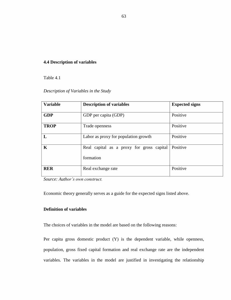
63
4.4 Description of variables
Table 4.1
Description of Variables in the Study
Variable Description of variables Expected signs
GDP GDP per capita (GDP) Positive
TROP Trade openness Positive
L Labor as proxy for population growth Positive
K Real capital as a proxy for gross capital
formation
Positive
RER Real exchange rate Positive
Source: Author’s own construct.
Economic theory generally serves as a guide for the expected signs listed above.
Definition of variables
The choices of variables in the model are based on the following reasons:
Per capita gross domestic product (Y) is the dependent variable, while openness,
population, gross fixed capital formation and real exchange rate are the independent
variables. The variables in the model are justified in investigating the relationship

64
between trade openness and economic growth in Namibia. GDP per capita growth (Y)
measures the performance of the economy from low productivity towards high
productivity, which can be related to their trade specialisation. A positive sign is
expected for this variable.
Trade openness (TROP) is captured by using trade share ratio (export / import) / GDP
as a measure of openness. This approach calculates trade openness used by
Osabbuohien (2007), Matadeen et al. (2011), Stensnes (2006) and Ahmad and Mohebbi
(2012). There are other measures available for trade openness, but this measure captures
qualitative and quantitative restrictions directly related with trade level to the rest of the
world. According to theory openness is positively related to economic growth, hence it
increases markets for new products by allowing market forces to allocate resources to
productive sectors which leads to efficiency and makes use of scale of economies. A
positive sign is expected for this variable.
Real exchange rate (RER) is the main determinate of the balance of payment (BoP) of
the nation in reference to its position and external competiveness. It is a useful resource
between tradable and non-tradable goods. Exchange rate also influences resource
allocation (Dornbuch et al 2004). This follows the works of lopez and Thirlwall (2004),

65
Nguyan (2008) and Yeboah et al (2012). A positive sign is expected. This is
complemented by Labour (L) (proxied by population growth).
Data on labour force is not readily available, thus population growth is used. An
increase of human capital may encourage capital accumulation and Real capital (K)
(proxied by real fixed capital formation) can be measured as private sector investment
in percentage of GDP. They are important factors in determining economic growth
according to the standard production function in the traditional economic theory. A
positive sign is expected for this variable as shown from various works earlier reviewed
(Mataden et al. 2011 and Obaden & Okojike, 2010).
Capital formation data is important in growth of Namibia in that investing in
infrastructure can contribute significantly to both private and public sectors in potential
sectors like Tourism, Mining, Fishing and Agriculture just to mention a few. Investing
in infrastructure adds value to economy and creates job opportunities by attracting more
investment thereby entering into new emerging markets which leads to diversification
in its export markets. A positive sign is expected for this variable as shown from various
works earlier reviewed. (Adhikary, 2011)
66
The measurement of trade openness in international trade is associated with exchange
controls, licenses, prohibition, quotas and tariff to mention a few. Edward (1998)
mentioned that black market share has been associated with trade restrictions such as
coverage of qualitative restrictions (QRs), tariff average and collected tariff ratios
(CTR) defined as ratio of tariff revenues to imports. Levine and Renelt (1992) and
Sachs and Warner (1995) used black market premium, the value is averaged in foreign
exchange rate market and used as overall extent of external sector distortions as a
proxy. The following measurement were used by Edward (1998), average import tariff
on manufacturing was measured as average import tariff and heritage foundation index
of distortion in international trade was measured as trade distortion through government
policies 1 to 5 values were taken as index. Furthermore, collected trade taxes ratio was
measured as total revenues taxes on trade (import + export) to total trade. In Leamer’s
(1998) openness index was measured as average residuals of trade flows regression,
while Sach’s and Warmer open index was measured as weighted average of changes in
domestic prices is equal to the trade reforms. Finally, the world development report
outward orientation index is classified according to their degree of openness which has
four categories.
The variables used are fundamental to the endogenous growth theory which illustrates
that a country with more open trade should concentrate on sectors where it has
comparative advantage. According to Romer (1989) a long run equilibrium growth rate
67
can be obtained through reduced cost of inputs and increased specialization. Trade
openness is also known to improve efficiency inputs allocation through technological
progress thereby eliminating protection on industries imports substitution. This results
improved economic growth (Solow, 1957). In another development, Edward (1998)
argues that trade openness does not improve the growth rate of poorer countries, but
rather through cost of imitation and knowledge of its initial stock. Moreover, Levine
and Renelt (1992) also urged the positive link between trade openness and economic
growth reporting that increased trade openness leads to lower real exchange rate and
higher inflation which impacts the domestic investment negatively, while Krugman
(1994) argues that amount of tariff and non-tariff barriers which is the degree of trade
openness affects only the volume of trade, not the link between imports, exports and
economic growth. In theoretical literature both the classical and neo-classical growth
models mention that capital is linked to economic growth. In other words, should there
be no capital, then investment will not be there and consequently there will be no
growth. While in empirical literature, Levine and Renelt and Harrison (1996) found a
positive link between investment share and trade share in GDP. In another development
Greenaway et al (2001) reported that higher export level led to an outward grading and
lower levels led an economy to an inward grading. Thus, the results confirmed that
openness led to growth because there was higher GDP growth in outward oriented
economies than inward oriented economies. Finally, exchange rate affects the
performance of the economy negatively should there be macroeconomic instability.
Lopez and Thirlwall (2004) reports that in liberalization process, exchange rate plays an

68
important role in the balance of payment by ensuring that imports do not exceed exports
if the country is to benefit effectively from trade.
However, different measurement of trade openness employed by researchers in a cross-
country analysis contribute to conflicting findings, According to Edward (1998)
openness results are affected by openness indicator, time period, functional form and
estimated technique. Moreover, Billmeier and Nannicini (2007) state that cross-country
estimators suffer from lack of transparency, while time series control for time invariant
unobservable characteristic of the country. Harrison (1996) used export +imports / GDP
suggested that this measure of trade openness is simply and mostly used as indicator.
Attention to this regard will be applied using a country data analysis to investigate the
linkage of trade openness and growth in Namibia with new evidence of literature.

69
CHAPTER FIVE: EMPIRICAL ANALYSIS AND RESULTS
5.1 Introduction
This chapter presents the empirical analysis and results of the study. The chapter is
organised as follows: Section 5.2 presents detailed estimation of variables which is
analyzed using techniques namely unit root test for stationarity, the vector error
correction model which estimates the Granger causality test, the impulse response
function that traces changes in each variable for current and future effect and the
variance decomposition, which estimates responses of variable shocks overtime.
5. 2: Detailed Estimations
5.2.1 Unit Root Tests
The statistical properties of the series in the study are first investigated through unit root
tests. Unit root tests help to test whether the series can provide correct inferences. In
standard economic theory, the stationarity test is important to ascertain that estimations
of regression are consistent. The unit root test applied the Augmented Dickey-Fuller
(ADF) and Phillips-Perron (PP) tests. The KPSS is estimated to confirm the tests since
the KPSS has much higher power limitation. The results of unit root test are presented
in Table 5.1.
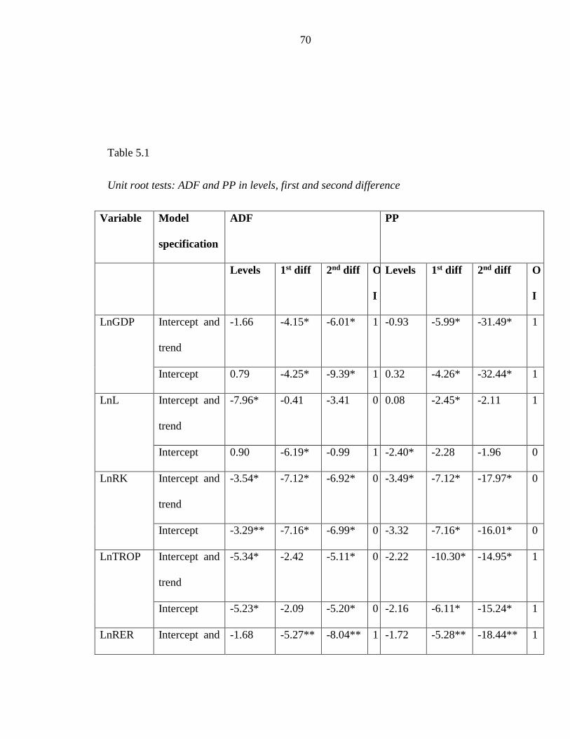
70
Table 5.1
Unit root tests: ADF and PP in levels, first and second difference
Variable Model
specification
ADF PP
Levels 1st diff 2nd diff O
I
Levels 1st diff 2nd diff O
I
LnGDP Intercept and
trend
-1.66 -4.15* -6.01* 1 -0.93 -5.99* -31.49* 1
Intercept 0.79 -4.25* -9.39* 1 0.32 -4.26* -32.44* 1
LnL Intercept and
trend
-7.96* -0.41 -3.41 0 0.08 -2.45* -2.11 1
Intercept 0.90 -6.19* -0.99 1 -2.40* -2.28 -1.96 0
LnRK Intercept and
trend
-3.54* -7.12* -6.92* 0 -3.49* -7.12* -17.97* 0
Intercept -3.29** -7.16* -6.99* 0 -3.32 -7.16* -16.01* 0
LnTROP Intercept and
trend
-5.34* -2.42 -5.11* 0 -2.22 -10.30* -14.95* 1
Intercept -5.23* -2.09 -5.20* 0 -2.16 -6.11* -15.24* 1
LnRER Intercept and -1.68 -5.27** -8.04** 1 -1.72 -5.28** -18.44** 1

71
trend
Intercept -2.57 -5.07** -8.19** 1 -2.55 -5.07** -18.87** 1
Source: Author’s compilation and values obtained from Eviews
Notes: (a) * mean the null hypothesis is rejected at 1%.
(b) ** mean the null hypothesis is rejected at 5%.
(c) *** mean the null hypothesis is rejected at 10%.
The null hypothesis is that there is presence of unit root. Table 5.1 show the results of
the ADF and PP test of all the variables in levels, first difference and second difference.
After testing the ADF test and the PP test in levels, it reveals that some variables like
LnGDP and LnRER are still non stationary in levels. After taking first difference, the
calculated ADF test and PP test rejected the null hypothesis of unit root when the
calculated ADF test and PP test statistics, is compared in relation to their critical values.
However, different order of integration is depicted. The KPSS test is another unit root
used to complement the ADF test and PP test.

72
Table 5.2
Unit root test: KPSS in levels and first difference
Variable Model Specification KPSS
Levels
First
Difference
Order of
integration
InGDP
Intercept and trend 0.19* 0.10** 0
Intercept 0.45** 0.62* 0
LnL
Intercept and trend 0.19* 0.12** 0
Intercept 0.74* 0.42* 0
InRK Intercept and trend 0.06** 0.08** 0
Intercept 0.14** 0.10** `0
InTROP Intercept and trend 0.14** 0.35 0
Intercept 0.64* 0.50* 0
InRER
Intercept and trend 0.18* 0.07** 0
Intercept 0.60* 0.39** 0
Source: Author’s compilation and values obtained from Eviews
Notes: (a) * mean the null hypothesis is rejected at 1%.
(b) ** mean the null hypothesis is rejected at 5%.

73
(c) *** mean the null hypothesis is rejected at 10%
The null hypothesis is that there is no unit root. This means that the null hypothesis for
KPSS can be rejected if the t-statistic computed is greater than the critical value. Table
5.2 shows the KPSS test that variables for the model are stationary in levels on all the
variables, therefore, this suggests that all the variables are integrated of the order 0.
5.2.2 Co-integration Test
Co-integration test is used in testing the linear combination of two or more time series.
When the series are more than one they link to form a long run relationship that is
possible even if individually they contain stochastic trend/non-stationary, as over time
they are assumed to move together and be stable and stationary (Granger,1990). In this
case, since the variables are integrated of the order one, variables are expected to have a
long run relationship. The Johansen test (Johansen-Juselius, 1990) was used. Table 5.3
below shows the Johansen co-integration test based on trace and maximum Eigen
values of the stochastic matrix.

74
Table 5.3
Johansen cointegration test based on Trace and Maximum Eigen Value test of the
Stochastic Matrix
Maximum Eigen Test Trace test
Ho:
rank=r
Ha:
rank=r
Statistics
5%
Critical
Value
Ho:
rank=r
Ha:
rank=r
Statistics
5%
Critical
Value
r = 0 r = 1 73.47** 33.88 r = 0 r ≥ 1 123.93** 69.82
r ≤ 1 r = 2 27.46 27.58 r ≤ 1 r ≥ 2 50.46** 47.86
r ≤ 2 r = 3 13.44 21.13 r ≤ 2 r ≥ 3 23.00 29.80
r ≤ 3 r = 4 7.09 14.26 r ≤ 3 r ≥ 4 9.57 15.50
r ≤ 4 r = 5 2.48 3.84 r ≤ 4 r ≥ 5 2.47 3.84
Source: Author’s compilation using Eviews.
Note: ** mean the null hypothesis is rejected at 5%.
The null hypothesis of co-integration states that there is no co-integration. In co-
integration testing, using the t-statistics indicates that the rejection of the null hypothesis
means that the calculated value of the test statistics is greater than the critical value,
meaning that the null hypothesis of no co-integration is rejected and concludes that
there is co-integration. Table 5.3 shows the trace test that the null hypothesis has been
rejected because the calculated t-statistics of 123.93 is greater than 69.82 of the critical
75
value and concludes that there is co-integration between the variables. Furthermore, the
test for Maximum Eigen value Test showed that one of the calculated values is greater
than the critical value at 5% significant level. This means that there more than one co-
integrating equation. Thus, a unique long run relationship exists among the variables
and tells us that output growth, trade openness, capital formation, labour force and
exchange rate are co-integrated. After co-integration results have been presented as
above, the VEC technique was used to estimate the regression for the Granger causality,
the impulse response function and the forecast error variance decomposition.
5.2.3 Vector Error Correction Model
After co-integration has been done, the restricted VAR, also known as the Vector error
correction model (VECM) is estimated when the variables are co-integrated. The VAR
procedure responds to how a change in one variable affects the future system or shows
forecasts of economic shocks (Engle & Granger, 1987). Furthermore, the VAR model
in this study is used to test the relationship between GDP per capita, trade openness,
capital formation, labor and exchange rate.
The restricted VAR was first applied to test the information on lag and how stable the
model is. The information on lag is shown below in Table 5.4
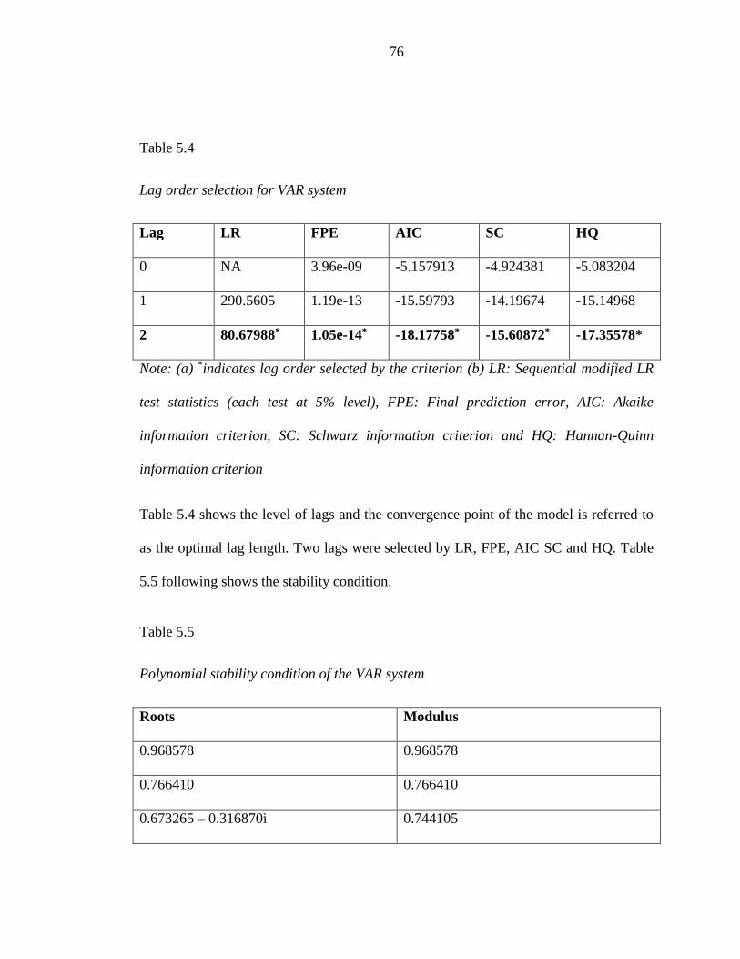
76
Table 5.4
Lag order selection for VAR system
Lag LR FPE AIC SC HQ
0 NA 3.96e-09 -5.157913 -4.924381 -5.083204
1 290.5605 1.19e-13 -15.59793 -14.19674 -15.14968
2 80.67988* 1.05e-14* -18.17758* -15.60872* -17.35578*
Note: (a) *indicates lag order selected by the criterion (b) LR: Sequential modified LR
test statistics (each test at 5% level), FPE: Final prediction error, AIC: Akaike
information criterion, SC: Schwarz information criterion and HQ: Hannan-Quinn
information criterion
Table 5.4 shows the level of lags and the convergence point of the model is referred to
as the optimal lag length. Two lags were selected by LR, FPE, AIC SC and HQ. Table
5.5 following shows the stability condition.
Table 5.5
Polynomial stability condition of the VAR system
Roots Modulus
0.968578 0.968578
0.766410 0.766410
0.673265 – 0.316870i 0.744105
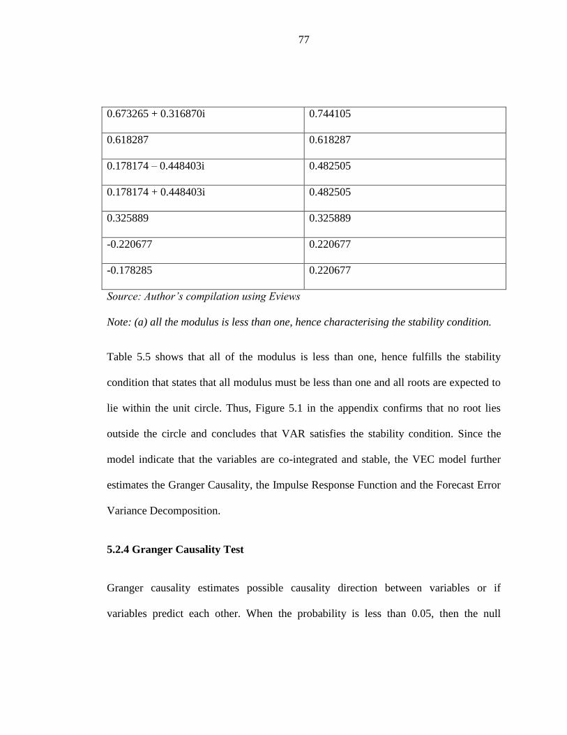
77
0.673265 + 0.316870i 0.744105
0.618287 0.618287
0.178174 – 0.448403i 0.482505
0.178174 + 0.448403i 0.482505
0.325889 0.325889
-0.220677 0.220677
-0.178285 0.220677
Source: Author’s compilation using Eviews
Note: (a) all the modulus is less than one, hence characterising the stability condition.
Table 5.5 shows that all of the modulus is less than one, hence fulfills the stability
condition that states that all modulus must be less than one and all roots are expected to
lie within the unit circle. Thus, Figure 5.1 in the appendix confirms that no root lies
outside the circle and concludes that VAR satisfies the stability condition. Since the
model indicate that the variables are co-integrated and stable, the VEC model further
estimates the Granger Causality, the Impulse Response Function and the Forecast Error
Variance Decomposition.
5.2.4 Granger Causality Test
Granger causality estimates possible causality direction between variables or if
variables predict each other. When the probability is less than 0.05, then the null
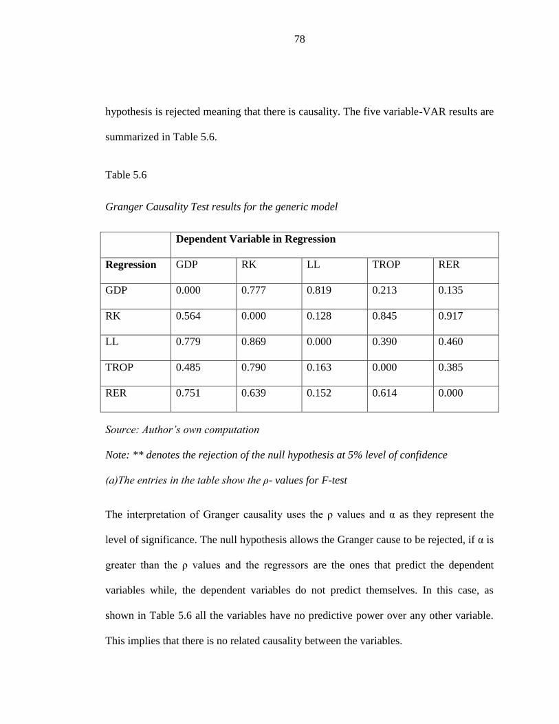
78
hypothesis is rejected meaning that there is causality. The five variable-VAR results are
summarized in Table 5.6.
Table 5.6
Granger Causality Test results for the generic model
Dependent Variable in Regression
Regression GDP RK LL TROP RER
GDP 0.000 0.777 0.819 0.213 0.135
RK 0.564 0.000 0.128 0.845 0.917
LL 0.779 0.869 0.000 0.390 0.460
TROP 0.485 0.790 0.163 0.000 0.385
RER 0.751 0.639 0.152 0.614 0.000
Source: Author’s own computation
Note: ** denotes the rejection of the null hypothesis at 5% level of confidence
(a)The entries in the table show the ρ- values for F-test
The interpretation of Granger causality uses the ρ values and α as they represent the
level of significance. The null hypothesis allows the Granger cause to be rejected, if α is
greater than the ρ values and the regressors are the ones that predict the dependent
variables while, the dependent variables do not predict themselves. In this case, as
shown in Table 5.6 all the variables have no predictive power over any other variable.
This implies that there is no related causality between the variables.

79
5.2.5 Impulse Response Function
The Impulse Response Function plots time paths difference between variables. The
Generalised Impulse Response Function (GIRF) shows how GDP reacts to exogenous
shocks in TROP, L, RK and RER. The GIRF capture multivariate models for both
linear and nonlinear unlike the Cholesky Impulse Function where variables are sensitive
to the ordering. Figure 5.2 below illustrates the response of GDP to the shocks in real
GDP, trade openness, capital formation, labor and real exchange rate.
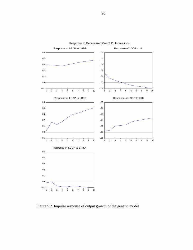
80
Figure 5.2. Impulse response of output growth of the generic model
-.01
.00
.01
.02
.03
.04
.05
1 2 3 4 5 6 7 8 9 10
Response of LGDP to LGDP
-.01
.00
.01
.02
.03
.04
.05
1 2 3 4 5 6 7 8 9 10
Response of LGDP to LL
-.01
.00
.01
.02
.03
.04
.05
1 2 3 4 5 6 7 8 9 10
Response of LGDP to LRER
-.01
.00
.01
.02
.03
.04
.05
1 2 3 4 5 6 7 8 9 10
Response of LGDP to LRK
-.01
.00
.01
.02
.03
.04
.05
1 2 3 4 5 6 7 8 9 10
Response of LGDP to LTROP
Response to Generalized One S.D. Innovations

81
Figure 5.2 shows the response of GDP to the shocks in TROP, RK, L and RER. As
illustrated in the graph, a shock to real GDP leads to a mild fall in the first three years
above the steady state. In the fourth year and onwards, it peaks up and maintains a
positive equilibrium state above the steady state from .03 in the initial year to .04. In the
long run, the effects of shock tend to wear out and GDP moves in a horizontal manner.
The shock to trade openness (TROP) leads to a sharp increase in GDP in the second
year reaching the steady state, and then declines sharply in the third year below the
steady state. In the long run, the effects of shock tend to wear out and GDP continues to
moves in a decreasing manner below the steady state. This implies that trade openness
shows negative effect to economic growth. This does not conform to expectation as the
neoclassical theory states that trade have a positive impact on the level of income.
However, the decrease in trade is confirmed in a report by the World Bank (2013) that
Namibia’s import exceeds its exports and trade has remained unchanged since 1990 at
55 to 60% of total GDP. Furthermore, efforts to grow the manufacturing industry is yet
to take root, while the main primary export in form of minerals has declined due to
global spillover have negatively affected its trade growth.
The impact of capital formation (RK) on GDP shows a sharp increase in economic
growth from the first year onwards at .00 to .02 in the tenth year. This shows a positive

82
impact to economic growth. In the long run, the effects of shock turn to wear out and
GDP moves in a horizontal manner. The results conform to theoretical expectation. The
output equation of Cobb-Douglas production function implies increasing returns to
capital and labour. This means that as investment increases, the higher will be the
output growth. Furthermore, a suggestion on increased capital for infrastructure in the
manufacturing industry so as to increase value on exported goods will also increase
output growth for Namibia. According to a report by World Bank (2012) Namibia has
seen a decline in ranking from 42nd among 175 countries to 78th among 183 countries.
A shock in labour (L) lends to a sharp decrease in GDP above the steady state up to the
fourth year. The fall continues gradually until it reaches the steady state equilibrium in
the fourth year, but continues to fall onwards until the tenth year. This suggests that
labour force has a negative impact to economic growth. In the long run GDP moves in a
decreasing manner. The outcome is not in line with the expectation in neoclassical
production function, where skills or education is a public good and one does not prevent
others from obtaining it. This means that when researchers interact amongst each other
this result in increased productivity and growth. In this case, more investment in
education is needed to improve the skilled labour in Namibia, which is in line with
vision 2030.
83
The shock in real exchange rate leads to an increase in economic growth from the first
year and by the second year it shows a decrease, then picks up in the third year and
continues to increase above the steady state. In the long run, it moves in the horizontal
manner from .00 in the first year to .04 in the tenth year. This implies a positive effect
to economic growth as expected. Real exchange rate volatility plays an important role to
Namibia in real value transfer of intra SACU revenues. If the real exchange rate
appreciates then the real value reduces and vice versa, hence the transfers in turn affect
the real GDP growth of Namibia.
Consequently, it is noted that a shock in three variables namely trade openness, capital
formation and real exchange rate showed an increase in first year before decreasing, but
capital formation maintained an upward trend, while real exchange rate and capital
formation in the long run move in a positive manner above the steady state. This shows
that there is a negative, but significant relationship between trade openness and
economic growth. In addition, to further uncover the interrelationship of variables and
movement with time, the forecast error variance decomposition test is done.
5.2.6 Forecast Error Variance Decomposition
The forecast error variance decomposition (FEVD) is used so as to achieve the forecast
ability and how each variable is important in random innovation using the VAR model.
The FEVD results are illustrated in Table 5.7.
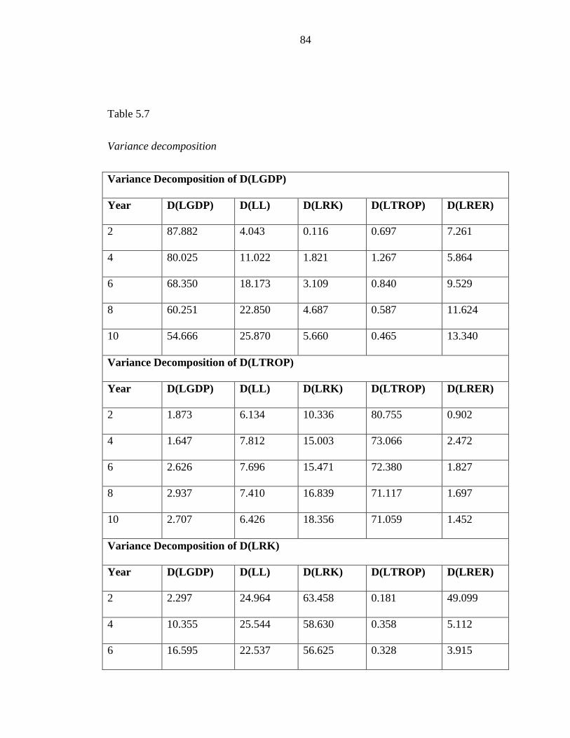
84
Table 5.7
Variance decomposition
Variance Decomposition of D(LGDP)
Year D(LGDP) D(LL) D(LRK) D(LTROP) D(LRER)
2 87.882 4.043 0.116 0.697 7.261
4 80.025 11.022 1.821 1.267 5.864
6 68.350 18.173 3.109 0.840 9.529
8 60.251 22.850 4.687 0.587 11.624
10 54.666 25.870 5.660 0.465 13.340
Variance Decomposition of D(LTROP)
Year D(LGDP) D(LL) D(LRK) D(LTROP) D(LRER)
2 1.873 6.134 10.336 80.755 0.902
4 1.647 7.812 15.003 73.066 2.472
6 2.626 7.696 15.471 72.380 1.827
8 2.937 7.410 16.839 71.117 1.697
10 2.707 6.426 18.356 71.059 1.452
Variance Decomposition of D(LRK)
Year D(LGDP) D(LL) D(LRK) D(LTROP) D(LRER)
2 2.297 24.964 63.458 0.181 49.099
4 10.355 25.544 58.630 0.358 5.112
6 16.595 22.537 56.625 0.328 3.915
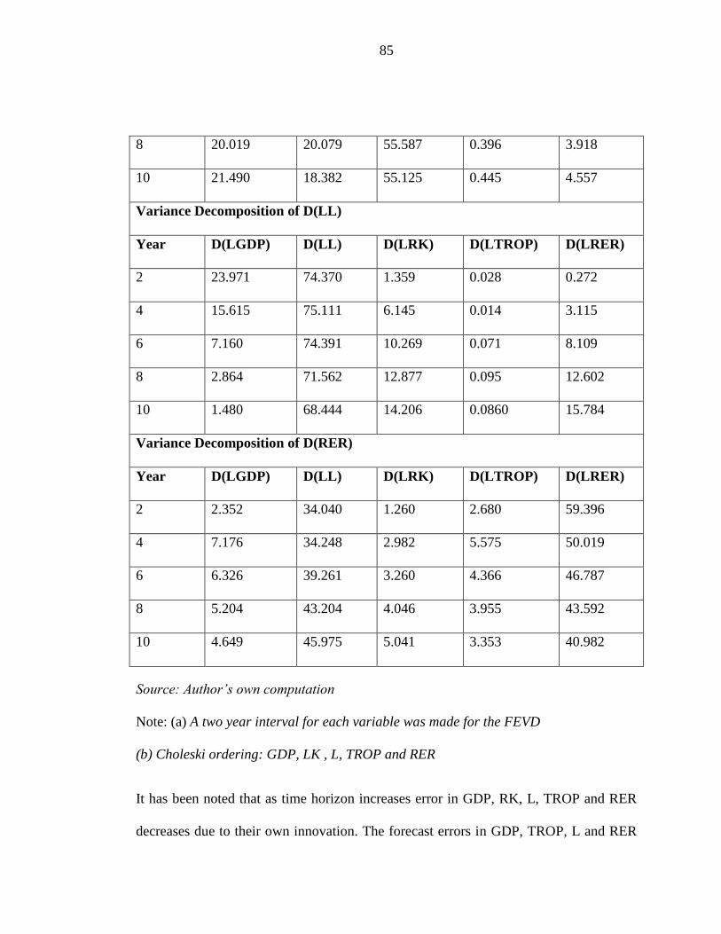
85
8 20.019 20.079 55.587 0.396 3.918
10 21.490 18.382 55.125 0.445 4.557
Variance Decomposition of D(LL)
Year D(LGDP) D(LL) D(LRK) D(LTROP) D(LRER)
2 23.971 74.370 1.359 0.028 0.272
4 15.615 75.111 6.145 0.014 3.115
6 7.160 74.391 10.269 0.071 8.109
8 2.864 71.562 12.877 0.095 12.602
10 1.480 68.444 14.206 0.0860 15.784
Variance Decomposition of D(RER)
Year D(LGDP) D(LL) D(LRK) D(LTROP) D(LRER)
2 2.352 34.040 1.260 2.680 59.396
4 7.176 34.248 2.982 5.575 50.019
6 6.326 39.261 3.260 4.366 46.787
8 5.204 43.204 4.046 3.955 43.592
10 4.649 45.975 5.041 3.353 40.982
Source: Author’s own computation
Note: (a) A two year interval for each variable was made for the FEVD
(b) Choleski ordering: GDP, LK , L, TROP and RER
It has been noted that as time horizon increases error in GDP, RK, L, TROP and RER
decreases due to their own innovation. The forecast errors in GDP, TROP, L and RER
86
have been increasing with time horizon due to their own innovation except in RER by
TROP and in L by GDP where it has been decreasing as time horizon increases.
Furthermore, the forecast errors in GDP by L, RER and RK increased as time horizon
increases. As such the variance of growth rate is at 100% in the first year. In the fourth
year, the variance decomposed in GDP growth rate by its own variance (80.02%)
followed by labour (11.02%), real exchange rate (5.86%) and capital formation
(1.27%). Furthermore, in the tenth year, the GDP growth rate is approximately constant
at 55% followed by labour at 26%, real exchange rate and capital formation (13% and
6% respectively). However, trade openness share in explaining the variation of real
GDP indicates a gradual increase from the second to fourth year, then decrease from the
sixth year onwards maintaining a constant 0%. In conclusion, the GDP growth rate
volatility is usually caused by its own variation, accounting for the majority portion of
the fluctuations (more than 50%).
87
CHAPTER SIX: CONCLUSION AND POLICY IMPLICATION
6.1 Conclusion
The study investigates the relationship between trade openness and economic growth in
Namibia using annual time series data for a period 1980 to 2011. In investigating the
relationship between trade openness and economic growth in the Namibian economy;
openness, capital formation, labour and exchange rate are used as explanatory variables
while GDP per capita is the dependent variable in VEC model. Based on stationarity
test results using ADF test and PP test showed some variables were stationary in levels,
some in first difference and one variable in second difference. Since variables were
stationary in different orders, the KPSS test was used to complement the results and
stationarity at 5% level of significant for the variable was found and integrated of order
1.
Co-integration test estimated and confirmed that a unique long run relationship exists
among the variables. Furthermore, the VEC model estimated the Granger causality
results showed that there is no related causality between variables, suggesting no long
run causal relationship between trade openness and economic growth. Shocks in real
exchange rate and capital formation showed they affect economic growth. However, the
effect of the shocks in real exchange rate, capital formation and GDP per capita itself

88
tend to wear out in the long run. While labour and trade openness affected economic
growth negatively.
Furthermore, the variance decomposition analysed that the GDP growth rate volatility
accounts for the majority portion caused by its own variation followed by labour, real
exchange rate, capital formation and the least was trade openness. This implies that
trade openness provide little importance in relation to capital formation in changing
GDP growth rate in Namibia.
6.2 Discussion of the result and Policy Implication
The positive impact of real exchange, capital formation and GDP per capita on
economic growth is stated by the neoclassical theory. This positive influence of capital
formation on GDP growth is similar to the study of Levine & Renalt (1992) and
Adhikary (2011). However, trade openness reveals a negative and insignificant sign on
changes to GDP growth. The evidence contradicts our positive theoretical expectation.
Perhaps, this is due to higher importation of goods than exports and the exportation of
mainly primary products with less value addition, hence the deficit in trade balance. The
study by Doric and Golley (2004) confirms that specializing in primary exportation has
a negative effect for growth which results in little benefit for developing economies in
trade.
89
There exists no related causal relationship between trade openness to GDP growth. The
lagged response in capital formation and exchange rate variables reveals a positive and
significant effect on changes in GDP growth of Namibia. The results are in line with the
theoretical literature of neoclassical theory of linkage between variables and similar to
findings of Yamada (1998), Kohpaiboon (2003) and Adhikary (2011). Kohpaiboon
(2003) states that FDI (in relation to exchange rate) has greater impact on growth under
export-led trade regime in relation to an import substitution regime. Yamada (1998)
confirms that adopting export oriented policies that promote labour-intensive industries
and investments that create job opportunities for the poor people also leads to economic
growth for the country. Furthermore, the variance decomposition analyzed that the GDP
growth rate volatility accounts for the majority portion caused by its own variation
followed by labour, real exchange rate, capital formation, and lastly trade openness.
Trade openness provides little importance in relation to capital formation and labour in
changing GDP growth rate in Namibia. Yamada (1998) found similar results on capital
formation and supports the effective policy in improving industrial sectors to boost the
economy of the country. The following recommendations are made:
The policy implication of this study are: since labour is the strongest
determinant of economic growth, the government should invest more in capital
infrastructure to boost investment which brings about new technology and
educational development to increase economic growth, with the resultant benefit
of employment creation and poverty reduction.
90
Improvement on manufacturing sector with labour-intensive output so as to
promote exports, create employment thereby reduces poverty.
Trade-led policies would be necessary to improve exports and discourage
imports especially on primary products were demand are inelastic.
6.3 Area for Further Research
The thesis reviews theoretical and empirical literature on the economic effects of trade
on growth. The primary focus of the report is the relationship between growth and trade.
A critical assessment of the literature still needs to be made along indications above, as
well as are several empirical explorations of the relationship between international trade
and economic growth arising from the assessment. Economic theory generally supports
the conclusion that trade has a positive effect on economic growth. Theorists disagree as
to whether increases in the growth rate of a country’s economy after a single episode of
trade lasts forever. Among the unresolved issues in such researches is the appropriate
quantitative measurement of “openness” and the variables used in estimation.

91
References
Adhikary, K.B. (2011). FDI, trade openness, capital formation, and economic growth in
Bangladesh: A linkage analysis. International Journal of Business and
Management, 6(1), 16-28.
Ahmadi, R., & Mohebbi, N. (2012). Trade openness and economic growth in Iran.
Journal of Basic and Applied Scientific Research, 2(1), 885-890.
Alif, A., & Ahmed, H. (2012). Impact of trade openness on output growth:
cointegration and error correction model approach. International Journal of
Economics and Finance, 2(4), 379-385.
Bajwa, S., & Siddiqui, W. M. (2011). Trade openness and its effects on economic
growth in selected South Asian countries: A panel data study. World Academy of
Science, Engineering and Technology, 50, 1073-1078.
Banga, R. (2003). Impact of government policies and investment agreements on FDI
inflows. American Journal of Agricultural Economics, 85 (5) 1140-1146
Bank of Namibia. (2012). Annual reports. Windhoek, Namibia.
Bleaney, M., & Greenaway, D. (2001). The impact of terms of trade and real exchange
rate volatility on investment and growth in Sub-Saharan Africa. Journal of Development
Economics, 65(2), 491-500.

92
Billmeier, A., & Nannicini, T. (2007). Trade openness and growth: Pursuing empirical
Glasnost. (International Monetary Fund Working Paper WP/07/156).
Capolupo, R., & Celi, G. (2008). Openness and economic growth: A comparative study
of alternative trading regimes. International Economics, 116, 5-36.
Cobb, C. W., & Douglas, P. H. (1928). A theory of production. American Economic
Review 18(1), 139–165.
Dickey, D. A., & Fuller, W. A. (1979). Distribution of the estimators for autoregressive
time series with a unit root. Journal of the American Statistical Association, 74,
427-431.
Din, M. (2004). Exports, imports and economic growth in South Asia: Evidence using a
multivariate time-series framework. The Pakistan Development Review, 43(2),
105-124.
Dobre, C. (2008). The relation between openness to trade and economic growth.
Retrieved July 8, 2013 from Central and Eastern European Online Library:
http://www.ceeol.com.
Dollar, D., & Kraay, A. (2002). Growth is good for the poor. Journal of Economic
Growth, 7, 195-225.
Dornbusch, R., Fishcher, S., & Startz, R. (2004). Macroeconomics, (9th ed.). Mc Graw-
Hill/Irwin.

93
Eboreime, M., & Iyoko, E. I. (2009). Causality between globalization and economic
growth: empirical evidence from Nigeria. Journal of Research in National
Development, 7(1).
Edward, S. (1998). Openness, productivity and growth: What do we really know? The
Economic Journal, 108, 383-398.
Ekanayake, E.M. (1999). Exports and economic growth in Asian developing countries:
Cointegration and error-correction models. Journal of Economic Development.
24(2), 43.
Enders, W. (2004). Applied econometrics: Time series. (2nd ed.). Wiley.
Engle, R., & Granger, C. (1987). Co-integration and error correction: Representation,
Estimation and Testing. Econometrica, 55(2), 251–276.
Garrett, G. (2001). Globalization and government spending around the world. Studies in
Comparative International Development, 35, 3-29.
Government Republic of Namibia (2006). Export processing zone. Ministry of Trade
and Industry. Windhoek.
Government Republic of Namibia (1993). To make provision for the promotion of
foreign investment in Namibia. Foreign investment act. Windhoek.
Granger, C. W. J. (1986). Developments in the study of cointegrated economic
variables. Oxford Bulletin of Economics and Statistics, 1(48), 213-228.
94
Grassman, G., & Hoolpman, E. (1990). Comparative advantage and long-run growth.
American Economic Review, 80, 796-815.
Greenaway, D., Morgan,W., & Wright, P. (2002). Trade liberalisation and growth in
developing countries. Journal of Development Economics, 67, 229–244.
Gujarati, D. N. (2003). Basic econometrics (4th ed.). McGraw-Hill, Inc.
Harrison, A. (2006). Globalization and poverty. ((National Bureau of Economic
Research Working Paper 12347). Cambridge: USA.
Harrison, A. (1996). Openness and growth: A time series, cross-country analysis for
developing countries. Journal of Development Economics, 48, 419-447.
Hassan, K.A.F.M., & Islam, R.M. (2005). Temporal causality and dynamics of financial
development, trade openness and economic growth in Vector Auto Regression
(VAR) for Bangladesh, 1974-2003: Implication for poverty reduction. The
Journal of Nepalese Business Studies, 2(1), 1-12.
Irwin, D.A., & Tervio, M. (2000). Does trade raise income? Evidence from the
twentieth century. (National Bureau of Economic Research Working Paper
7745). Cambridge: USA.
Johansen, S. (1988). Statistical analysis of cointegration vectors. Journal of Economic
Dynamics and Control, 12(2), 231– 254.
95
Jordaan, A.C., & Eita, J.H. (2007). Export and economic growth in Namibia: A granger
causality analysis. South African Journal of Economics 75(3), 540-547.
Kakar, Z.K., & Khilji, B.A. (2011). Impact of FDI and trade openness on economic
growth: A comparative study of Pakistan and Malaysia. Theoretical and Applied
Economics, 18(11), 53-58.
Kanyenze, G., & Lapeyre, F. (2012). Growth, employment and decent work in
Namibia: A situation analysis. (ILO Employment Working Paper 81). Geneva:
Switzerland.
Kohpaiboon, A. (2003). Foreign trade regime and the FDI-Growth nexus: A case study
of Thailand. Journal of Development Studies, 40(2), 55-69.
Koopman,T. C. (1965). On the concept of economic growth in the econometric
approach to development. Chicago, Rand-McNally.
Krugman, P. (1994). The myth of Asia’s miracle. Foreign Affairs, 73(6), 63-78.
Krugman, P. (1986). Strategic trade policy and the new international economics.
Cambridge. MA: The MIT press.
Krugman, P.R. (1979). Increasing returns, monopolistic competition and international
trade. Journal of International Economics 9(4): 469-479.
Kwiatkowski, D., Phillips, P.C., Schmidt, P., & Shin, Y. (1992). Testing the null
hypothesis of stationarity against the alternative of a unit root: how sure are we

96
that economic time series have a unit root? Journal of Econometrics, 54(1), 159-
178.
Levine, R., & Renelt, D. (1992). A sensitivity analysis of cross-country growth
regressions. The American Economic Review, 82(4), 942-963.
Lopez, P. P., & Thirlwall, A.P. (2004). Trade liberalization in Mexico: Rhetoric and
reality. (School of Economics Working Paper no. 04.03). University of Kent:
UK.
Lucas, R. E. (1988). On the Mechanics of economic development. Journal of Monetary
Economics 22(1) 3-42
Matadeen, J., Matadeen, S. J., & Seetanah, B. (2011, December). Trade openness and
economic growth: Evidence from Mauritius. International Conference on
International Trade and Investment, University of Mauritius.
Namibia Statistics Agency. (2012). Annual trade statistics bulletin. Retrieved October
20, 2013, from http://www.nsa.org.na
Nashiidi, E., & Ogbokor, A. C. (2013). Testing the long run relationship between export
and economic growth: evidence from Namibia. Journal of Emerging Issues in
Economics, Finance and Banking, 1(5).
National Planning Commission. (2013). National accounts: 2004-2012, Central Bureau
of Statistics: Windhoek.

97
National Planning Commission, (2012). Fourth national development plan (NDP4).
Windhoek: National Planning Commission.
Nowbutsing, M. B., Ramsohok, K., & Ramsohok, S. (2012). Impact of openness on
economic growth: Case of Indian Ocean rim countries. Retrieved October 15,
2013, from University of Mauritius, library web site:
http://site.uom.ac.mu/wtochair/imges/stories/cproceedings12/Boboo M
Nowbutsing Sonalisinh Ramsohok The impact of Openness on Economic Growth
Case of Indian Ocean Rim Countries Final. pdf
Obadan, I. M., & Okojie, I. E. (2010). An empirical analysis of the impact of trade on
economic growth in Nigeria. JOS Journal of Economics, 4(1).
Odada, J. E., & Matundu, O. K. (2008). China-Africa economics relations: The case of
Namibia. University of Namibia, Department of Economics. Published by
African Economic Research Consortium (AERC).
Ogbokor, C. A. (2005). Macroeconomic impact of trade on Namibian growth: An
empirical illustration. Journal of Social Sciences, 1(1), 57-60.
Osabuohien, S. C. E. (2007). Trade openness and economic performance of ECOWAS
members-reflections from Ghana and Nigeria. African Journal of Business and
Economics Research, 2(3), 57-73.
Pesaran, M. H., & Yongcheol, S. (1998). Generalized impulse response analysis in
linear multivariate models. Economics Letters 58, 17-29.
98
Phillips, P., & Perron, P. (1988). Testing for a unit root in time series regression.
Biometrika, 75(2), 335–346.
Ramsey, F. P. (1928). A mathematical theory of saving. Economic Journal, 38 (152),
543-559.
Ray, S. (2012). Determinants of total factor productivity growth in selected
manufacturing industries in India. Research and Social Practices in Social
Sciences, 7(2), 25-43.
Rigobon, R., & Rodrik, D. (2004). Rule of law, democracy, openness, and income:
Estimating the interrelationships. (National Bureau of Economic Research
Working Papers 10750,). Cambridge: USA.
Rivera, M.A., & Romer, P.M. (1990). Economic integration and endogenous growth.
(National Bureau of Economic Research Working Papers 3528). Cambridge:
USA.
Rodriguez, F. (2006). Openness and growth: What have we learned? (Wesleyan
Economics Working Paper 2006-011). Connecticut: USA.
Rodrik, D., Subramanian, A., & Trebbi, F. (2004). Institutions rule: The primacy of
institutions over geography and integration in economic development. Journal
of Economic Growth, 9, 131-165.
Romer, P.M. (1990). Endogenous technological change. Journal of Political Economy,
98(5), 71-102.
99
Romer, P. M. (1986). Increasing returns and long-run growth. Journal of Political
Economy, 94(5), 1002-1037.
Sachs, J.D., & Warner, A. (1995). Economic reform and the process of global
integration. (Brookings papers on Economic Activity 1).
Salvastor, D. (2007). International Economics. (9th ed.). Wiley.
Sarkar, P. (2007). Trade openness and growth: Is there any link? (MPRA working
paper no. 4997). Munich: Germany.
Sheefeni, J.P.S. (2013). Testing for the Fisher hypothesis in Namibia. Journal of
Emerging Issues in Economics, Finance and Banking 2(1), 571-582.
Sherbourne, R. (2009). Guide to Namibian Economy. Institute for Public Policy
Research. Embassy of Finland, Windhoek.
Solow, R. M. (1956). A contribution to the theory of economic growth. The Quarterly
Journal of Economics 70(1) 65-94.
Southern African customs union. (2010/11).Annual report 2010/11,Windhoek,
Namibia. Author.
Southern African Customs Union. (2012). Annual report 2012, Windhoek, Namibia.
Author.
Stensnes, K. (2006). Trade openness and economic growth: Do institutions matter?
Norwegian Institute of International, 702.

100
Trading Economics. (2013). Retrieved June 08, 2013 from
www.tradeingeconomics.com/country
United Nations Development Programme. (2011). Namibia’s aid for trade framework
and strategy. Windhoek: UNDP.
United States Trade Representative. (n.d.). Namibia. Retrieved May 15, 2013 from
http://www.ustr.gov/countries-regions/africa/southern-africa/namibia.
Vamvakidis, A. (2002). How Robust is the growth-openness connection: Historical
evidence. Journal of Economic Growth, 7(1), 57-80.
Vohra, R. (2001). Export and economic growth: Further time series evidence from less
developed countries. International Advances in Economic Research, 7(3), 345-
350.
Webster, J. T. (2003). Managerial economics: Theory and practice, (9th ed.). Academic
Press.
World Bank (2013). World development report indicators 2013, Retrieved February 13,
2013 from http://www.wto.org
World Bank. (2012). World Development Indicators [CD]. New York: Author.
World Bank (2012). World development report 2012, Retrieved February 13, 2013 from
http:// www.wto.org.

101
World Bank (2010). World development report indicators 2010, Retrieved February 13,
2013 from http://www.wto.org.
Yamada, H. (1998). A note on the causality between export and productivity: An
empirical re-examination. Economic Letters, 61(2), 111-114.
Yanikkaya, H. (2003). Trade openness and economic growth: a cross-country empirical
investigation. Journal of Development Economic, 72(1), 57-89.
Yeboah, O., Naanwaab, C., Saleem, S., & Akuffo, A. (2012, February). Effects of trade
openness on economic growth: The case of African countries. Southern
Agricultural Economics Association Annual Meeting, Birmingham, AL.
Yucel, F. (2009). Causal relationship between financial development, trade openness
and economic growth: The case of Turkey. Journal of Social Sciences, 5(1), 33-
42.
Zulfiqar, K., & Kausar, R. (2012). Trade liberalization, exchange rate and export
growth in Pakistan. Far East Journal of Psychology and Business, 9(2), 32.

102
Appendix
Table 3.1: Selected Studies on Trade Openness
Study author, date Measure of
trade
/openness
Variables used Countries Findings
Levine and Renelt,
1992
Trade / GDP
ratio
Per capita GDP,
Openness,
Government
consumption
/GDP, Inflation,
Population, Arable
land per worker
92 countries (past
four decades)
Period: past four
decades
Indirect impact between trade openness and
economic growth through investment and
productivity.
Harrison, 1996 Black Capital stock, 51 countries No evidence of relationship between trade
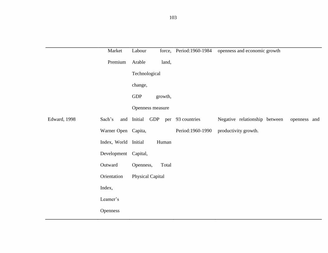
103
Market
Premium
Labour force,
Arable land,
Technological
change,
GDP growth,
Openness measure
Period:1960-1984 openness and economic growth
Edward, 1998 Sach’s and
Warner Open
Index, World
Development
Outward
Orientation
Index,
Leamer’s
Openness
Initial GDP per
Capita,
Initial Human
Capital,
Openness, Total
Physical Capital
93 countries
Period:1960-1990
Negative relationship between openness and
productivity growth.
104
Index,
Average
Black
Market,
Average
Input tariff
on
Manufacturin
g,
Average
coverage of
non Tariff
Barriers,
Heritage
Foundation
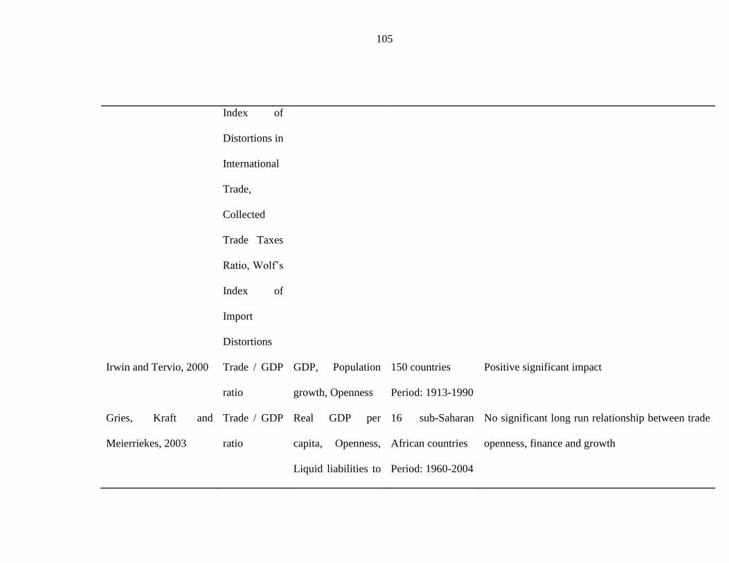
105
Index of
Distortions in
International
Trade,
Collected
Trade Taxes
Ratio, Wolf’s
Index of
Import
Distortions
Irwin and Tervio, 2000 Trade / GDP
ratio
GDP, Population
growth, Openness
150 countries
Period: 1913-1990
Positive significant impact
Gries, Kraft and
Meierriekes, 2003
Trade / GDP
ratio
Real GDP per
capita, Openness,
Liquid liabilities to
16 sub-Saharan
African countries
Period: 1960-2004
No significant long run relationship between trade
openness, finance and growth

106
GDP, Private credit
to GDP
Hassan and Islam, 2005 Trade / GDP
ratio
Openness, Private
credit, Domestic
credit, Real GDP
Bangladesh
Period: 1974-2003
Bi-directional causal relationship between
financial development, trade openness and growth
Osabuohien, 2007 Trade / GDP
ratio
Per capita GDP,
Real government
expenditure,
Labour force, Real
capital stock,
Openness
Ghana and
Nigeria
Period: 1975-2004
Positive impact between trade openness and
economic growth
Sakar, 2007 Trade / GDP
ratio
GDP per capita,
Openness
51 countries
Period: 1981-2002
Less developed countries showed no positive long
term relationship. Middle income countries
experienced a positive long term relationship
between trade openness and economic growth

107
Adhikery, 2011 Trade / GDP
ratio
Real GDP, capital
formation, FDI,
Openness,
Bangladesh
Period: 1986-2008
Negative and diminishing effect between trade
openness and GDP growth rate
Yeboah et al, 2012 Trade / GDP
ratio
FDI, Exchange
rate, Capital-
Labour ratio, Trade
openness
38 countries
Period: 1980-2008
Positive relationship between trade openness and
GDP growth
Source: Author’s own construct
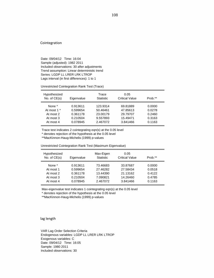
108
Cointegration
Date: 09/04/12 Time: 16:04
Sample (adjusted): 1982 2011
Included observations: 30 after adjustments
Trend assumption: Linear deterministic trend
Series: LGDP LL LRER LRK LTROP
Lags interval (in first differences): 1 to 1
Unrestricted Cointegration Rank Test (Trace) Hypothesized Trace 0.05
No. of CE(s) Eigenvalue Statistic Critical Value Prob.** None * 0.913611 123.9314 69.81889 0.0000
At most 1 * 0.599654 50.46461 47.85613 0.0278
At most 2 0.361178 23.00179 29.79707 0.2460
At most 3 0.210504 9.557893 15.49471 0.3163
At most 4 0.078945 2.467072 3.841466 0.1163 Trace test indicates 2 cointegrating eqn(s) at the 0.05 level
* denotes rejection of the hypothesis at the 0.05 level
**MacKinnon-Haug-Michelis (1999) p-values
Unrestricted Cointegration Rank Test (Maximum Eigenvalue) Hypothesized Max-Eigen 0.05
No. of CE(s) Eigenvalue Statistic Critical Value Prob.** None * 0.913611 73.46683 33.87687 0.0000
At most 1 0.599654 27.46282 27.58434 0.0518
At most 2 0.361178 13.44390 21.13162 0.4122
At most 3 0.210504 7.090821 14.26460 0.4785
At most 4 0.078945 2.467072 3.841466 0.1163 Max-eigenvalue test indicates 1 cointegrating eqn(s) at the 0.05 level
* denotes rejection of the hypothesis at the 0.05 level
**MacKinnon-Haug-Michelis (1999) p-values
lag length
VAR Lag Order Selection Criteria
Endogenous variables: LGDP LL LRER LRK LTROP
Exogenous variables: C
Date: 09/04/12 Time: 16:05
Sample: 1980 2011
Included observations: 30

109
Lag LogL LR FPE AIC SC HQ 0 82.36870 NA 3.96e-09 -5.157913 -4.924381 -5.083204
1 263.9690 290.5605 1.19e-13 -15.59793 -14.19674 -15.14968
2 327.6637 80.67988* 1.05e-14* -18.17758* -15.60872* -17.35578* * indicates lag order selected by the criterion
LR: sequential modified LR test statistic (each test at 5% level)
FPE: Final prediction error
AIC: Akaike information criterion
SC: Schwarz information criterion
HQ: Hannan-Quinn information criterion
AR Root (Stability)
Roots of Characteristic Polynomial
Endogenous variables: LGDP LL LRER LRK LTROP
Exogenous variables: C
Lag specification: 1 2
Date: 09/04/12 Time: 16:05 Root Modulus 0.968578 0.968578
0.766410 0.766410
0.673265 - 0.316870i 0.744105
0.673265 + 0.316870i 0.744105
0.618287 0.618287
0.178174 - 0.448403i 0.482505
0.178174 + 0.448403i 0.482505
0.325889 0.325889
-0.220677 0.220677
-0.178285 0.178285 No root lies outside the unit circle.
VAR satisfies the stability condition.
Granger Causality
VEC Granger Causality/Block Exogeneity Wald Tests
Date: 09/04/12 Time: 16:06
Sample: 1980 2011

110
Included observations: 29
Dependent variable: D(LGDP) Excluded Chi-sq df Prob. D(LL) 0.398417 2 0.8194
D(LRER) 4.004418 2 0.1350
D(LRK) 0.505354 2 0.7767
D(LTROP) 3.090749 2 0.2132 All 6.653426 8 0.5744
Dependent variable: D(LL) Excluded Chi-sq df Prob. D(LGDP) 0.500134 2 0.7787
D(LRER) 1.554148 2 0.4597
D(LRK) 0.280510 2 0.8691
D(LTROP) 1.884747 2 0.3897 All 4.346481 8 0.8246
Dependent variable: D(LRER) Excluded Chi-sq df Prob. D(LGDP) 0.571648 2 0.7514
D(LL) 3.763442 2 0.1523
D(LRK) 0.894362 2 0.6394
D(LTROP) 0.976224 2 0.6138 All 6.688068 8 0.5706
Dependent variable: D(LRK) Excluded Chi-sq df Prob. D(LGDP) 1.145827 2 0.5639
D(LL) 4.111337 2 0.1280
D(LRER) 0.174440 2 0.9165
D(LTROP) 0.336398 2 0.8452 All 6.420690 8 0.6002
Dependent variable: D(LTROP)

111
Excluded Chi-sq df Prob. D(LGDP) 1.447145 2 0.4850
D(LL) 3.626367 2 0.1631
D(LRER) 1.910142 2 0.3848
D(LRK) 0.471304 2 0.7901 All 5.233777 8 0.7323
Impulse Response Test
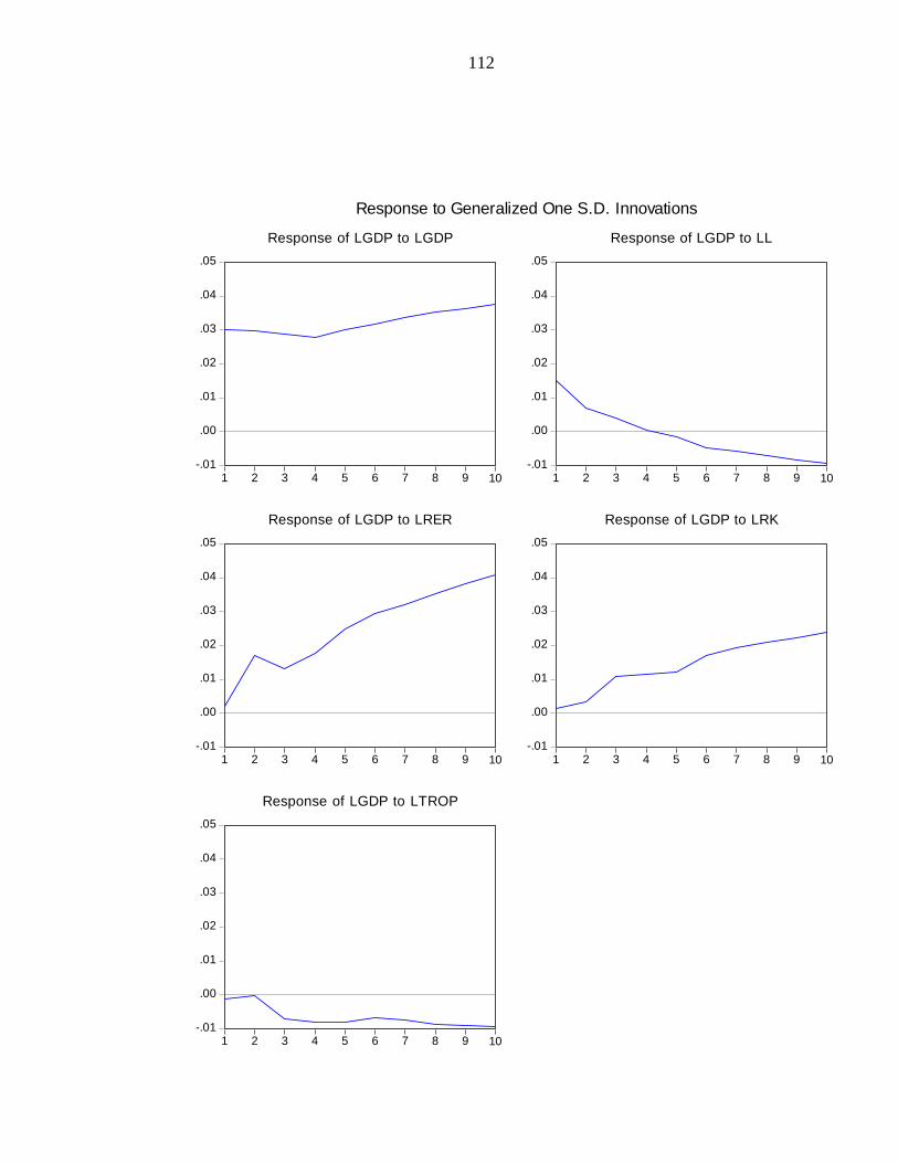
112
-.01
.00
.01
.02
.03
.04
.05
1 2 3 4 5 6 7 8 9 10
Response of LGDP to LGDP
-.01
.00
.01
.02
.03
.04
.05
1 2 3 4 5 6 7 8 9 10
Response of LGDP to LL
-.01
.00
.01
.02
.03
.04
.05
1 2 3 4 5 6 7 8 9 10
Response of LGDP to LRER
-.01
.00
.01
.02
.03
.04
.05
1 2 3 4 5 6 7 8 9 10
Response of LGDP to LRK
-.01
.00
.01
.02
.03
.04
.05
1 2 3 4 5 6 7 8 9 10
Response of LGDP to LTROP
Response to Generalized One S.D. Innovations

113
Variance Decomposition Test
Varian
ce Decomposition
of LGDP:
Period S.E. LGDP LL LRER LRK LTROP 1 0.030096 100.0000 0.000000 0.000000 0.000000 0.000000
2 0.045054 87.88210 4.043503 7.261286 0.115611 0.697496
3 0.055534 84.67344 7.412754 5.589566 1.243211 1.081025
4 0.064972 80.02531 11.02171 5.864280 1.821572 1.267127
5 0.075831 74.34968 14.52295 7.920131 2.123120 1.084110
6 0.087898 68.35002 18.17261 9.528796 3.109021 0.839552
7 0.100131 63.87433 20.80250 10.62750 4.019105 0.676569
8 0.112660 60.25099 22.85020 11.62440 4.687064 0.587344
9 0.125222 57.19175 24.51578 12.55952 5.210377 0.522576
10 0.137736 54.66578 25.86982 13.34026 5.659387 0.464748 Varian
ce Decomposition of LL:
Period S.E. LGDP LL LRER LRK LTROP 1 0.000527 25.14421 74.85579 0.000000 0.000000 0.000000
2 0.001770 23.97072 74.37038 0.272201 1.359133 0.027573
3 0.003859 20.48908 74.51665 1.237290 3.750560 0.006422
4 0.006801 15.61464 75.11125 3.115044 6.145325 0.013734
5 0.010570 10.90496 75.12338 5.560303 8.369030 0.042322
6 0.015060 7.160452 74.39111 8.108623 10.26862 0.071201
7 0.020115 4.527285 73.11787 10.49946 11.76645 0.088932
8 0.025559 2.863589 71.56221 12.60227 12.87708 0.094848
9 0.031222 1.928112 69.95051 14.36297 13.66580 0.092610
10 0.036960 1.480158 68.44371 15.78382 14.20633 0.085985 Varian
ce Decomposition
of LRER:
Period S.E. LGDP LL LRER LRK LTROP 1 0.144267 0.419554 34.03961 65.54084 0.000000 0.000000
2 0.198778 2.351691 34.31217 59.39612 1.260088 2.679930
3 0.245651 5.806893 33.05826 52.67443 2.654965 5.805450
4 0.279456 7.176024 34.24816 50.01931 2.981635 5.574869
5 0.307933 6.970122 36.98951 48.00711 3.220144 4.813112
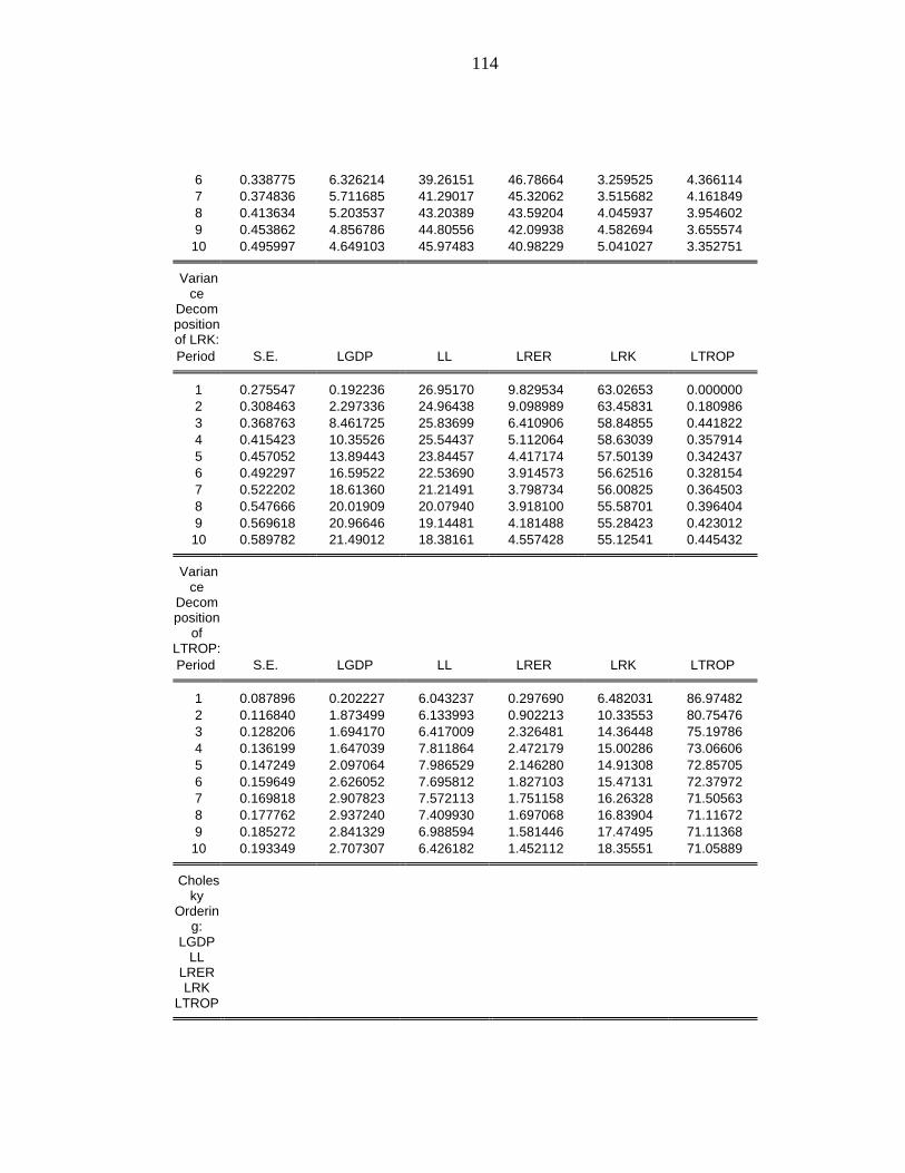
114
6 0.338775 6.326214 39.26151 46.78664 3.259525 4.366114
7 0.374836 5.711685 41.29017 45.32062 3.515682 4.161849
8 0.413634 5.203537 43.20389 43.59204 4.045937 3.954602
9 0.453862 4.856786 44.80556 42.09938 4.582694 3.655574
10 0.495997 4.649103 45.97483 40.98229 5.041027 3.352751 Varian
ce Decomposition of LRK:
Period S.E. LGDP LL LRER LRK LTROP 1 0.275547 0.192236 26.95170 9.829534 63.02653 0.000000
2 0.308463 2.297336 24.96438 9.098989 63.45831 0.180986
3 0.368763 8.461725 25.83699 6.410906 58.84855 0.441822
4 0.415423 10.35526 25.54437 5.112064 58.63039 0.357914
5 0.457052 13.89443 23.84457 4.417174 57.50139 0.342437
6 0.492297 16.59522 22.53690 3.914573 56.62516 0.328154
7 0.522202 18.61360 21.21491 3.798734 56.00825 0.364503
8 0.547666 20.01909 20.07940 3.918100 55.58701 0.396404
9 0.569618 20.96646 19.14481 4.181488 55.28423 0.423012
10 0.589782 21.49012 18.38161 4.557428 55.12541 0.445432 Varian
ce Decomposition
of LTROP:
Period S.E. LGDP LL LRER LRK LTROP 1 0.087896 0.202227 6.043237 0.297690 6.482031 86.97482
2 0.116840 1.873499 6.133993 0.902213 10.33553 80.75476
3 0.128206 1.694170 6.417009 2.326481 14.36448 75.19786
4 0.136199 1.647039 7.811864 2.472179 15.00286 73.06606
5 0.147249 2.097064 7.986529 2.146280 14.91308 72.85705
6 0.159649 2.626052 7.695812 1.827103 15.47131 72.37972
7 0.169818 2.907823 7.572113 1.751158 16.26328 71.50563
8 0.177762 2.937240 7.409930 1.697068 16.83904 71.11672
9 0.185272 2.841329 6.988594 1.581446 17.47495 71.11368
10 0.193349 2.707307 6.426182 1.452112 18.35551 71.05889 Choles
ky Orderin
g: LGDP
LL LRER LRK
LTROP
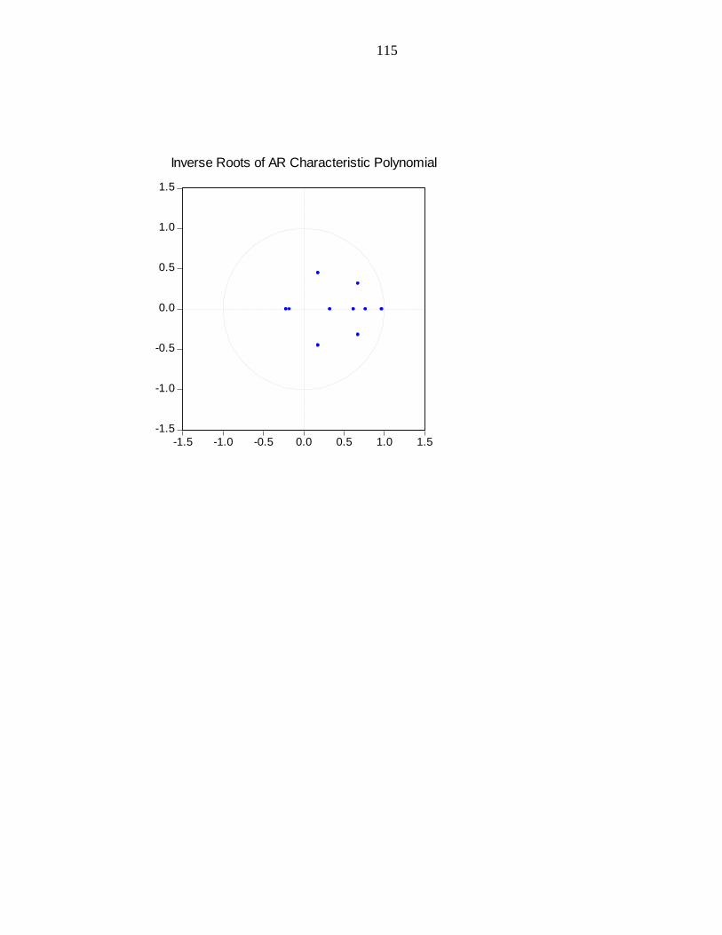
115
-1.5
-1.0
-0.5
0.0
0.5
1.0
1.5
-1.5 -1.0 -0.5 0.0 0.5 1.0 1.5
Inverse Roots of AR Characteristic Polynomial