an optimal gear design method for minimization of transmission error and vibration excitation

The Pennsylvania State University

The Graduate School

Department of Acoustics

AN OPTIMAL GEAR DESIGN METHOD FOR MINIMIZATION

OF TRANSMISSION ERROR AND VIBRATION EXCITATION

A Dissertation in

Acoustics

by

Cameron P. Reagor

c© 2010 Cameron P. Reagor

Submitted in Partial Fulfillmentof the Requirements

for the Degree of

Doctor of Philosophy

May 2010

The dissertation of Cameron P. Reagor was reviewed and approved* by the following:

William D. MarkSenior Scientist, Applied Research LaboratoryProfessor Emeritus of AcousticsDissertation AdviserChair of Committee

Stephen A. HambricSenior Scientist, Applied Research LaboratoryProfessor of Acoustics

Gary H. KoopmannDistinguished Professor of Mechanical Engineering

Victor W. SparrowProfessor of AcousticsInterim Chair of the Graduate Program in Acoustics

*Signatures are on file in the Graduate School.

iii

Abstract

Fluctuation in static transmission error is the accepted principal cause of vibration

excitation in meshing gear pairs and consequently gear noise. More accurately, there are

two principal sources of vibration excitation in meshing gear pairs: transmission error

fluctuation and fluctuation in the load transmitted by the gear mesh. This dissertation

formulates the gear mesh vibration excitation problem in such a way that explicitly

accounts for the aggregate contributions of these excitation components. The Fourier

Null Matching Technique does this by imposing a constant value on the transmission error

and solving for the requisite contact region on a tooth surface that yields a constant load

transmitted by the gear mesh. An example helical gear is created to demonstrate this

approach and the resultant compensatory geometry. The final gear tooth geometry is

controlled in such a way that modifications to the nominal involute tooth form exactly

account for deformation under load across a range of loadings. Effectively, the procedure

adds material to the tooth face to control the contact area thereby negating the effects of

deformation and deviation from involute. To assess the applicability of the technique, six

deformation steps that correlate to loads ranging from light loading to the approximate

full loading for steel gears are used. A nearly complete reduction in transmission error

fluctuations for any given constant gear loading should result from the procedure solution.

This overall method should provide a substantial reduction in the resultant vibration

excitation and consequently, noise.

iv

Table of Contents

List of Tables . . . . . . . . . . . . . . . . . . . . . . . . . . . . . . . . . . . . . . vii

List of Figures . . . . . . . . . . . . . . . . . . . . . . . . . . . . . . . . . . . . . viii

Acknowledgments . . . . . . . . . . . . . . . . . . . . . . . . . . . . . . . . . . . xv

Chapter 1. Introduction . . . . . . . . . . . . . . . . . . . . . . . . . . . . . . . . 1

Chapter 2. Previous Research . . . . . . . . . . . . . . . . . . . . . . . . . . . . 3

2.1 History of Gearing . . . . . . . . . . . . . . . . . . . . . . . . . . . . 3

2.2 Noise in Gearing . . . . . . . . . . . . . . . . . . . . . . . . . . . . . 4

2.3 Current Gear Noise State of the Art . . . . . . . . . . . . . . . . . . 8

2.4 Development of a Complete Solution . . . . . . . . . . . . . . . . . . 8

2.5 Present Work . . . . . . . . . . . . . . . . . . . . . . . . . . . . . . . 10

Chapter 3. Preliminaries . . . . . . . . . . . . . . . . . . . . . . . . . . . . . . . 12

3.1 Gearing Constructs . . . . . . . . . . . . . . . . . . . . . . . . . . . . 13

3.2 Mathematical Preliminaries . . . . . . . . . . . . . . . . . . . . . . . 15

3.2.1 The Involute Curve . . . . . . . . . . . . . . . . . . . . . . . . 15

3.2.2 Angle Relations . . . . . . . . . . . . . . . . . . . . . . . . . . 16

3.2.3 Gear Coordinates . . . . . . . . . . . . . . . . . . . . . . . . . 22

3.2.4 Regular Gear Relations . . . . . . . . . . . . . . . . . . . . . 24

3.3 Transmission Error . . . . . . . . . . . . . . . . . . . . . . . . . . . . 25

3.4 The Tooth Force Equation . . . . . . . . . . . . . . . . . . . . . . . . 26

Chapter 4. The Main Procedure . . . . . . . . . . . . . . . . . . . . . . . . . . . 30

4.1 Bounding the Problem . . . . . . . . . . . . . . . . . . . . . . . . . . 30

4.2 The Role of Convolution in Gear Noise . . . . . . . . . . . . . . . . . 32

4.3 Convolution’s Relation to Gear Geometry . . . . . . . . . . . . . . . 36

4.4 Developing the Procedure . . . . . . . . . . . . . . . . . . . . . . . . 37

4.5 Applying Fourier Principles . . . . . . . . . . . . . . . . . . . . . . . 39

4.6 Extending the Contact Region . . . . . . . . . . . . . . . . . . . . . . 41

4.6.1 The First Step . . . . . . . . . . . . . . . . . . . . . . . . . . 41

v

4.6.2 Continuing the Expansion . . . . . . . . . . . . . . . . . . . . 42

4.7 Fourier Null Matching Technique . . . . . . . . . . . . . . . . . . . . 44

4.8 Practical Work Flow . . . . . . . . . . . . . . . . . . . . . . . . . . . 48

Chapter 5. The Results . . . . . . . . . . . . . . . . . . . . . . . . . . . . . . . . 52

5.1 Test Gear Parameters . . . . . . . . . . . . . . . . . . . . . . . . . . 52

5.2 The Test Gear . . . . . . . . . . . . . . . . . . . . . . . . . . . . . . 54

5.3 Compliance and Loading . . . . . . . . . . . . . . . . . . . . . . . . . 57

5.4 Contact Region . . . . . . . . . . . . . . . . . . . . . . . . . . . . . . 70

5.5 Endpoint Modification . . . . . . . . . . . . . . . . . . . . . . . . . . 78

5.6 Discussion of Computed Contact Regions . . . . . . . . . . . . . . . 89

Chapter 6. Summary and Conclusions . . . . . . . . . . . . . . . . . . . . . . . . 92

6.1 The Fourier Null Matching Technique . . . . . . . . . . . . . . . . . 92

6.2 The Practicality of the Tooth Modification . . . . . . . . . . . . . . . 93

6.3 Limitations of the Analysis . . . . . . . . . . . . . . . . . . . . . . . 93

6.4 Extending the Process . . . . . . . . . . . . . . . . . . . . . . . . . . 95

6.5 Closure . . . . . . . . . . . . . . . . . . . . . . . . . . . . . . . . . . 96

Appendix A. Notation . . . . . . . . . . . . . . . . . . . . . . . . . . . . . . . . . 97

Appendix B. Derivations . . . . . . . . . . . . . . . . . . . . . . . . . . . . . . . 100

B.1 Simplifying the Load Angle Equation . . . . . . . . . . . . . . . . . . 100

B.2 Radius of Curvature . . . . . . . . . . . . . . . . . . . . . . . . . . . 101

Appendix C. The Analysis Primary Code . . . . . . . . . . . . . . . . . . . . . . 104

C.1 Main . . . . . . . . . . . . . . . . . . . . . . . . . . . . . . . . . . . . 104

C.2 Gear Design Control . . . . . . . . . . . . . . . . . . . . . . . . . . . 106

C.3 Parameter Setup . . . . . . . . . . . . . . . . . . . . . . . . . . . . . 108

C.4 Initiate the Finite Element Programs . . . . . . . . . . . . . . . . . . 110

C.5 Initialize the Finite Element Analysis . . . . . . . . . . . . . . . . . . 110

C.6 Set the Location Constants . . . . . . . . . . . . . . . . . . . . . . . 111

C.7 Open Saved Progress File . . . . . . . . . . . . . . . . . . . . . . . . 113

C.8 Graph the Legendre Loading Coefficients . . . . . . . . . . . . . . . . 115

C.9 Develop the Element Positions . . . . . . . . . . . . . . . . . . . . . 116

C.10 Map the Loading Profile on the Current Element Set . . . . . . . . . 119

C.11 Find the Hertzian Width . . . . . . . . . . . . . . . . . . . . . . . . . 121

vi

C.12 Mesh the Finite Element Model . . . . . . . . . . . . . . . . . . . . . 123

C.13 Perform the Finite Element Analysis . . . . . . . . . . . . . . . . . . 139

C.14 Apply Forces to the Finite Element Model . . . . . . . . . . . . . . . 140

C.15 Execute the Finite Element Analysis . . . . . . . . . . . . . . . . . . 142

C.16 Read the Finite Element Data . . . . . . . . . . . . . . . . . . . . . . 143

C.17 Prepare the Finite Element Data for Plotting . . . . . . . . . . . . . 146

C.18 Solve the Compliance Matrix . . . . . . . . . . . . . . . . . . . . . . 147

C.19 Reset the Loading Data . . . . . . . . . . . . . . . . . . . . . . . . . 149

C.20 Save the Critical Iteration Data . . . . . . . . . . . . . . . . . . . . . 150

C.21 Determine the Boundary of the Unmodified Region . . . . . . . . . . 150

C.22 Determine the Edge Extension . . . . . . . . . . . . . . . . . . . . . 153

C.23 Determine Step Size . . . . . . . . . . . . . . . . . . . . . . . . . . . 160

C.24 Apply Default Loading . . . . . . . . . . . . . . . . . . . . . . . . . . 162

C.25 Open A Saved Data Set . . . . . . . . . . . . . . . . . . . . . . . . . 163

C.26 Rotate the Node Plane . . . . . . . . . . . . . . . . . . . . . . . . . . 164

References . . . . . . . . . . . . . . . . . . . . . . . . . . . . . . . . . . . . . . . . 165

vii

List of Tables

5.1 Test Design Gear . . . . . . . . . . . . . . . . . . . . . . . . . . . . . . . 52

5.2 Test Design Gear Continued . . . . . . . . . . . . . . . . . . . . . . . . . 53

5.3 Summary of αΩ(N/µm). . . . . . . . . . . . . . . . . . . . . . . . . . . . 68

5.4 Summary of Line of Contact End Points. All values in m. . . . . . . . . 77

A.1 Summary of General Gearing Notation . . . . . . . . . . . . . . . . . . . 97

A.2 Summary of Transmission Error Notation . . . . . . . . . . . . . . . . . 99

A.3 Summary of Optimization Notation . . . . . . . . . . . . . . . . . . . . . 99

viii

List of Figures

2.1 An example of meshing gear teeth is shown. The global pressure angle,

φ, the base radius, Rb, and the pitch radius, R are indicated. . . . . . . 4

2.2 An example transmission error profile is shown. The horizontal coordi-

nate can be thought of as roll distance as the gear rotates. The vertical

coordinate is the deviation from perfect transfer of rotational position

expressed at the tooth surface. 1.2 cycles of gear rotation are shown. . . 5

2.3 An example Fourier spectrum of the transmission error is shown. The

horizontal coordinate is the gear rotational harmonic. The vertical co-

ordinate is the amplitude of each rotational harmonic. The gear has 59

teeth. . . . . . . . . . . . . . . . . . . . . . . . . . . . . . . . . . . . . . 6

2.4 Crowning: Typically a single lead modification and a single profile mod-

ification, (a), linearly superimpose to give a crowned deviation from per-

fectly involute, (b). Material, as described in this deviation from involute,

is removed from the perfect involute tooth, (c), in a direction normal to

the tooth surface thereby forming the crowned tooth illustrated in (d). . 7

2.5 From left to right: Given a finite element mesh of a gear tooth, any

element in that mesh that has an applied load also has size constraints.

Any applied lineal load along the length of the element creates a Hertzian

contact region b and has a unique ratio of element height c to width e

associated with it that is required to accurately predict b. . . . . . . . . 10

3.1 Standard gear diagram showing the analysis gear below and the mating

gear above it. The base plane projection of this helical gear pair is shown

above the mating gears. From Mark [5]. . . . . . . . . . . . . . . . . . . 12

3.2 The involute curve, I, is traced by the end of a string unwrapped from

a cylinder (with radius Rb). The roll angle, ε, is the angle swept by

the point of tangency, T , for the string with the cylinder as the string

unwraps. The pressure angle, φ, is the angle of force for meshing gears. φ

is measured against the pitch plane (the horizontal plane perpendicular

to the plane containing the gear axis). The construction pressure angle,

φi, is equal to φ when the “string” is unwrapped to the pitch point, P ′. 14

ix

3.3 Dual Construction: for a set of local pressure angles, φi, locations on a

single tooth profile or multiple profiles rotating through space can satisfy

the resultant geometry. . . . . . . . . . . . . . . . . . . . . . . . . . . . . 15

3.4 The four gear planes: the transverse plane in blue, the pitch plane in

green, the axial plane in orange and the base plane in red. The mating

gear would be located directly above the gear cylinder for the gear of

analysis shown in dark blue. . . . . . . . . . . . . . . . . . . . . . . . . 16

3.5 A gear tooth (red) with its equivalent rack shown in blue and line of

contact in black. The green tooth profile intersects the line of contact at

the pitch point. . . . . . . . . . . . . . . . . . . . . . . . . . . . . . . . . 17

3.6 An involute curve (black) is commonly illustrated originating from the

horizontal or x-axis. . . . . . . . . . . . . . . . . . . . . . . . . . . . . . 18

3.7 θ′, as measured on the face of the equivalent basic rack tooth, is the angle

between the line of contact (magenta) and the base of the rack tooth.

The pressure angle, φ, is measured in the transverse plane. As measured

in the pitch plane, the pitch cylinder helix angle, ψ, is measured between

the tooth base normal and the transverse plane. φn is the elevation of

the tooth face normal. . . . . . . . . . . . . . . . . . . . . . . . . . . . . 19

3.8 While the roll angle, ε, can be broken up into its components, φi and

θi, the pressure angle, φi, can be further divided at the tooth thickness

median into βi and ιi. . . . . . . . . . . . . . . . . . . . . . . . . . . . . 20

3.9 The force that is incident on a gear tooth can be broken into three com-

ponents. The helix and pressure angles are evident. . . . . . . . . . . . 21

3.10 Gear tooth ranges, L and D, relative to tooth rotation. . . . . . . . . . 23

4.1 Frequency domain theoretical gear noise is bound to integer multiples of

the primary gear rotational harmonic (n = 1). A vast majority of the

noise power in real world gears is found here as well. . . . . . . . . . . 32

4.2 A unit square function (a) has a frequency spectrum (b) with zeros at

integer harmonics. A unit triangle function (c) which is the convolution

of two square functions also has a frequency spectrum (d) with zeros at

the same integer harmonics. Note the difference in the falloff of the two

spectra. . . . . . . . . . . . . . . . . . . . . . . . . . . . . . . . . . . . . 33

4.3 A narrow square function is convolved with a triangle function to create

a new rounded triangular function. . . . . . . . . . . . . . . . . . . . . 34

x

4.4 The convolution of two square functions can produce a triangle function

or a trapezoidal function (a). Either is a “second order” function that

has a Fourier transform with asymptotic falloff of f−2 in frequency (b).

A “third order” convolved function (c) will produce a Fourier asymptotic

falloff on the order of f−3 (d). . . . . . . . . . . . . . . . . . . . . . . . 35

4.5 A square function of width ε convolves with a triangular function of width

2∆ to form a new function with a third order Fourier asymptotic falloff. 36

4.6 The black box denotes the available area on a tooth surface. The grey

box denotes the nominal Qa = Qt = 1 contact region. This region is only

valid for very light loading. As the line of contact travels from s = −∆ to

s = ∆, the practical width of line within the grey-boxed contact region

behaves like a triangular function. The tooth root is located at small ε

and the tooth tip is located at the upper bound of ε. . . . . . . . . . . 40

4.7 The unmodified region of a line of contact, denoted by the flat area

at loading u′0, are extended on either side by some distance, θ1. This

distance corresponds to the first design loading, u′1. . . . . . . . . . . . . 42

4.8 The line of contact includes two extensions beyond the unmodified con-

tact region. The first step extends the range by θ1 on either end and the

second step extends the previous line length by θ2 at each end. . . . . . 43

4.9 An example Fourier transmission error spectrum is shown through the

25th tooth harmonic. . . . . . . . . . . . . . . . . . . . . . . . . . . . . . 45

4.10 An example continuous frequency noise spectrum is illustrated where

the noise energy is centered on integer multiples of the tooth meshing

fundamental. . . . . . . . . . . . . . . . . . . . . . . . . . . . . . . . . . 46

4.11 The frequency domain envelope of a Fourier Null Matching Technique

load profile is shown. . . . . . . . . . . . . . . . . . . . . . . . . . . . . . 46

4.12 An illustration of a Fourier Null Matching Technique resultant transmis-

sion error spectrum is shown. . . . . . . . . . . . . . . . . . . . . . . . . 47

4.13 An illustration of several lines of contact. The outer box represents the

available area on a tooth face. The inner box represents the Qa = Qt = 1

area which bounds the line of contact for −∆ ≤ s ≤ ∆. The step size

between lines of contact is ∆/4 in s while the horizontal coordinate is y

and the vertical coordinate is z. . . . . . . . . . . . . . . . . . . . . . . . 48

xi

4.14 The lower triangular figure represents the force transmitted by a single

tooth pair as they come in and out of contact. More completely, the total

force per unit depth deformation over a line of contact as a function of

s for each tooth-to-tooth cycle is represented as this triangle over the

range −∆ ≤ s ≤ ∆. The upper figure is the superimposed transmitted

forces of all tooth pairs. The total gear mesh transmitted load (sum of

the superimposed triangles) remains constant as the gear rotates. . . . . 49

4.15 A conceptual illustration of the nominal “lightly loaded” contact region

(bounded in blue) that satisfies Equation 4.13. Note that the initial rect-

angular region is not the bounds of the zone of contact that corresponds

to a triangular transmitted force profile. Several lines of contact are

shown in red. . . . . . . . . . . . . . . . . . . . . . . . . . . . . . . . . . 50

4.16 A conceptual illustration of the first expanded contact region (narrow

blue). The contact region that corresponds to regular transmitted force

profile (e.g. a triangle) is not regularly shaped itself (e.g. not rectangular). 51

5.1 A rendered example of the test gear. . . . . . . . . . . . . . . . . . . . 54

5.2 A closer view of the test gear showing the pitch point, P , and point of

tangency, T . . . . . . . . . . . . . . . . . . . . . . . . . . . . . . . . . . 55

5.3 A standard isometric view of the test gear. The pitch point, P , and point

of tangency, T are indicated. . . . . . . . . . . . . . . . . . . . . . . . . 55

5.4 An example of a finite element model used for the compliance analysis. 56

5.5 A close up of a finite element model used for the compliance analysis.

This model is for s = 0.8∆ . . . . . . . . . . . . . . . . . . . . . . . . . . 57

5.6 The loading curves for s = −0.008085 m . . . . . . . . . . . . . . . . . . 58

5.7 The loading curves for s = −0.0071866 m . . . . . . . . . . . . . . . . . 58


5.9 The loading curves for s = −0.00539 m . . . . . . . . . . . . . . . . . . . 59



5.12 The loading curves for s = −0.002695 m . . . . . . . . . . . . . . . . . . 61



5.15 The loading curves for s = 0 m . . . . . . . . . . . . . . . . . . . . . . . 62

5.16 The loading curves for s = 0.00089833 m . . . . . . . . . . . . . . . . . . 63

xii


5.18 The loading curves for s = 0.002695 m . . . . . . . . . . . . . . . . . . . 64



5.21 The loading curves for s = 0.00539 m . . . . . . . . . . . . . . . . . . . . 65



5.24 The loading curves for s = 0.008085 m . . . . . . . . . . . . . . . . . . . 67

5.25 The nominal loading case results in a perfect triangle. The remain-

ing load steps deviate slightly from a triangular profile. Note that the

rounded triangle is not immediately apparent due to resolution in s. . . 69

5.26 The bounds of each line of contact and its position on the tooth face is

shown in the same orientation as Figure 4.6 for deformation step u =

1µm. Blue box denotes Qa = Qt = 1. The lines of contact vary from

s = −0.9∆ on the lower right to s = 0.9∆ on the upper left with a step

between of ∆s = ∆/10. The tip of the tooth is positive z and the root

is negative z. . . . . . . . . . . . . . . . . . . . . . . . . . . . . . . . . . 70

5.27 The bounds of each line of contact for deformation step u = 5µm. Blue

box denotes Qa = Qt = 1. The lines of contact vary from s = −0.9∆

on the lower right to s = 0.9∆ on the upper left with a step between of

∆s = ∆/10. The tip of the tooth is positive z and the root is negative z. 71













xiii





5.32 The estimated contact region for the final geometry is seen. Note the well-

behaved portion of the tooth: negative s (lower right) for deformation

steps from 5 µm to 25 µm. . . . . . . . . . . . . . . . . . . . . . . . . . 76

5.33 Each line of contact is constrained to have symmetric adjustments to the

length of the line of contact for each deformation step. The positive-y

extension profile is a mirror of the negative-y deformation profile. . . . . 78

5.34 The positive y end point modifications for s = −0.00808 m for all defor-

mation cases. . . . . . . . . . . . . . . . . . . . . . . . . . . . . . . . . . 79


mation cases. . . . . . . . . . . . . . . . . . . . . . . . . . . . . . . . . . 79


mation cases. . . . . . . . . . . . . . . . . . . . . . . . . . . . . . . . . . 80


mation cases. . . . . . . . . . . . . . . . . . . . . . . . . . . . . . . . . . 80


mation cases. . . . . . . . . . . . . . . . . . . . . . . . . . . . . . . . . . 81


mation cases. . . . . . . . . . . . . . . . . . . . . . . . . . . . . . . . . . 81


mation cases. . . . . . . . . . . . . . . . . . . . . . . . . . . . . . . . . . 82


mation cases. . . . . . . . . . . . . . . . . . . . . . . . . . . . . . . . . . 82

5.42 The positive y end point modifications for s = −0.000898 m for all de-

formation cases. . . . . . . . . . . . . . . . . . . . . . . . . . . . . . . . . 83

5.43 The positive y end point modifications for s = 0 m for all deformation

cases. . . . . . . . . . . . . . . . . . . . . . . . . . . . . . . . . . . . . . 83

5.44 The positive y end point modifications for s = 0.000898 m for all defor-

mation cases. . . . . . . . . . . . . . . . . . . . . . . . . . . . . . . . . . 84


mation cases. . . . . . . . . . . . . . . . . . . . . . . . . . . . . . . . . . 84

xiv


mation cases. . . . . . . . . . . . . . . . . . . . . . . . . . . . . . . . . . 85


mation cases. . . . . . . . . . . . . . . . . . . . . . . . . . . . . . . . . . 85


mation cases. . . . . . . . . . . . . . . . . . . . . . . . . . . . . . . . . . 86


mation cases. . . . . . . . . . . . . . . . . . . . . . . . . . . . . . . . . . 86


mation cases. . . . . . . . . . . . . . . . . . . . . . . . . . . . . . . . . . 87


mation cases. . . . . . . . . . . . . . . . . . . . . . . . . . . . . . . . . . 87


mation cases. . . . . . . . . . . . . . . . . . . . . . . . . . . . . . . . . . 88

B.1 The solution of the radius analysis and the linear regression of the anal-

ysis are nearly collinear. . . . . . . . . . . . . . . . . . . . . . . . . . . . 103

xv

Acknowledgments

I am most grateful and indebted to my thesis advisor, Dr. William D. Mark, for

his generosity with guidance, patience, and encouragement that he has shown me here

at Penn State. I am especially indebted for the financial support which the Rotorcraft

Center has provided. I thank my other committee members, Drs. Gary Koopmann,

Stephen Hambric and Victor Sparrow, for their insightful commentary on my work. I

would also like to thank my wonderful wife, Sara, for her unyielding support over the

duration of this work. Her support has been essential to the completion of the techniques

contained herein.

1

Chapter 1

Introduction

From the inception of rotary machinery, gears have been manipulating and trans-

mitting power. From early wooden examples to modern involute drivetrains, gears have

been integral to the development of machinery and power manipulating technology. Most

modern gearing is conjugate [1], i.e. it is designed to transmit a constant rotational ve-

locity, and the involute tooth form [2] is the most common example of conjugate gearing.

Ideal involute gears transmit uniform rotational velocities without any error, but such

gears are not possible.

The displacement based exciter function known as the transmission error (T.E.)

[3, 4, 5, 6] is the accepted principal source for noise in involute gearing. In most gear

systems operating at speed, the load applied across the gear mesh dominates inertial

forces, and as such, the relative rotational position error of the meshing gears is directly

correlated to any vibration caused by the system. Excitation in the system is also

dependent upon the transmitted load. Put another way, an ideal gear pair would be able

to transmit a constant rotational velocity perfectly from the drive gear to the driven

gear under constant load conditions. For real gears, the difference in the position of

the output gear when compared to its ideal analog is the transmission error. This

transmission error can be directly traced to deviations from the perfect involute form

due to geometric differences and deformation under load.

There are two manifest requirements imposed upon a gearing system (tooth pro-

file) for transmission error fluctuations to be eliminated. One, the transmission error

must be constant through the range of the gear rotation for any mesh loading; and two,

the gear mesh must transmit a constant loading. These two fundamental quantities,

uniform force and velocity, govern the design of quiet gearing and bear on any design

consideration including stiffness, geometry or drivetrain layout.

The transmission error, as experienced in meshing gears, arises from two com-

ponents: geometric deviation from involute and deformations under load. Geometric

deviations can either be intentional or unintentional. Intentional deviations arise from

manufacturing modifications such as crowning or tip relief. Unintentional errors like

2

scalloping or improper finishing are also geometric deviations. Deformation across the

loaded tooth mesh also has two components. Both gross body compliance and Hertzian

compliance contribute to deformation under load. These deviations from the ideal in-

volute gear tooth surface for loaded gears are the primary cause of transmission error.

Eliminating or compensating for these deviation types can eliminate transmission error.

The purpose of this thesis is to describe a method for computing the optimal gear

and tooth design for the minimization of transmission error fluctuations and the mainte-

nance of constant transmitted gear mesh loading. This method is denoted as the Fourier

Null Matching Technique. Tooth geometry, tooth deformation, manufacturing error,

bearing stiffness and alignment must all be accounted for when tooth geometry is mod-

ified with the goal of reducing transmission error fluctuations for practical application.

The idealized case contained herein is the first step to a viable gear design.

The reduction of transmission error fluctuation requires the development of precise

compensatory gear geometry that, when loaded, accounts for all design and compliant

variations in the tooth-to-tooth meshing of a rotating gear pair. Effectively, material is

precisely added to the tooth face to exactly compensate for deformation under load. This

“zero sum” design should approach the performance of a rigid, ideal involute drivetrain

thereby transmitting a uniformly proportional rotational velocity, and thereby no trans-

mission error. In addition the total transmitted load across the gear mesh is held to be

constant. Careful control of the gear tooth geometry can extend this “zero sum” design

over a range of gear loadings. The final benefit of the Fourier Null Matching Technique

is that within the framework of maintaining constant transmitted load and transmis-

sion error, the frequency domain behavior of the meshing gear is such that the integer

bound tooth harmonics are eliminated by aligning the nulls of the frequency domain gear

tooth mesh behavior to the tooth meshing harmonics. The use of finite element analysis

(FEA), numerical optimization, linear algebra, and a variety of computational methods

are used in the solution of the “zero sum” gear design. The approach utilized herein is

believed to be novel.

3

Chapter 2

Previous Research

2.1 History of Gearing

Gears can be traced to the earliest machines. While the lever and wedge date

to the palaeolithic era [7], the other basic machines and engineering in the modern

sense can be historically traced to the Greeks [8]. Through surviving texts, Aristotle

and his followers are shown to have used and discussed the (gear-)wheel, the lever, the

(compound) pulley, the wedge and others. While limited by materials and analytical

techniques, simple machines and gears were used and continued to be developed and

considered by the Romans, the Arab world, and the Chinese [9]. From water clocks to

anchor hoists to catapults, the force-multiplying properties of gears were used by early

engineers throughout antiquity.

Though gears are simple in principle, their problems are far from trivial. In clocks

and windmills, gear wear was a significant problem and continued to be so throughout

the Renaissance. The mathematical and geometrical tools available to Renaissance en-

gineers were simply insufficient to solve the problem of the optimal gear tooth profile [8].

Leonhard Euler was the first to successfully attack the problem by showing that uniform

transfer of motion can be achieved by a conjugate and specifically, an involute profile [10].

While often ignored by his contemporaries due to being written in Latin and being highly

mathematical, Euler’s advances in planar kinematics and gearing in particular brought

modern gear analysis into existence.

While mechanical clocks drove the proliferation of gearing in the 15th and 16th

centuries, the industrial revolution brought an impetus to advance gearing in support of

the steam engine. By the end of the 18th century the Ecole Polytechnique was established

in Paris and the modern academic study of kinematics and machinery had begun [9]. The

increased need for power manipulation on larger scales that accompanied the industrial

revolution brought about an explosion of fundamentally modern gearing.

Metallurgical, lubricative, and analytical advances continued through the 19th

and 20th centuries, but the form of gearing remained largely unchanged. Not until the

4

analysis of transmission error began in earnest in the mid 20th century did the form of

gearing deviate from Euler’s ideal profile.

2.2 Noise in Gearing

As a practical matter, audible gear noise resulting from transmission error is

subject to a torturous path from the gear mesh to the ear. From a meshing gear pair,

vibration must pass through bearings, shafts, gear cases, machine structures, mounts,

and panelling before any noise can be heard [11]. This type of path varies in specifics

but generally holds for any modern transmission. The cyclical nature of gear contact

(see Figure 2.1), and thereby, gear noise is expressed as cyclical deviation of rotational

position in the time domain (see Figure 2.2) and as a series of harmonics related to the

error cycles in the frequency domain (see Figure 2.3).

Fig. 2.1. An example of meshing gear teeth is shown. The global pressure angle, φ, thebase radius, Rb, and the pitch radius, R are indicated.

5

100 200 300 400 500 600 700

−1

−0.5

0

0.5

1

1.5x 10

−3 Transmission Error

Basal Distance, x (mm)

Tra

nsm

issi

on E

rror

(m

m)

Fig. 2.2. An example transmission error profile is shown. The horizontal coordinatecan be thought of as roll distance as the gear rotates. The vertical coordinate is thedeviation from perfect transfer of rotational position expressed at the tooth surface. 1.2cycles of gear rotation are shown.

Common measures used to address gear noise are isolation and damping through-

out the gear vibration path. However, the root of the problem lies in the gear tooth

interaction and any attempt at broadly reducing gear noise must focus on that cause.

By the late 1930’s, Henry Walker [12] was able to state that the transmission error

was the primary cause of gear noise. As gear analysis progressed in the 20th century,

the transmission error became the accepted cause of gear noise [3]. In the 1970’s and

1980’s the transmission error was shown to be directly proportional to audible gear

noise [11, 13]. Transmission error is now universally accepted to be the source of gear

noise [14, 15, 16, 17, 13].

6

0 20 40 60 80 100 120 140

10−6

10−5

10−4

Fourier Transmission Error Spectrum

Gear Rotational Harmonic, n

Fou

rier

Mag

nitu

de (

mm

)

Fig. 2.3. An example Fourier spectrum of the transmission error is shown. The horizon-tal coordinate is the gear rotational harmonic. The vertical coordinate is the amplitudeof each rotational harmonic. The gear has 59 teeth.

Before rigorous analysis of involute gearing was available, gear noise was addressed

through rudimentary modification of the nominal involute tooth surface. This procedure

came to be known as crowning [18] or relief [19]. Tip relief is an effective tool to ensure

proper tooth clearance and nominal base plane action [14] which are critical to gear

noise [20]. In modern crowning, typically a single lead and a single profile modification are

combined and applied to the gear tooth surface. See the illustration in Figure 2.4. Axial

and profile crowning together [21, 22] have been shown to reduce gear noise in general and

address specific gearing issues such as misalignment. The addition of load computation,

mesh analysis, and line of contact constraints [23] have made the procedures’ results

robust and manufacturable.

Gear design for the minimization of gear noise, optimization of gear loading, and

maximization of manufacturability have been attempted throughout the field [24, 23, 19,

7

Fig. 2.4. Crowning: Typically a single lead modification and a single profile modifica-tion, (a), linearly superimpose to give a crowned deviation from perfectly involute, (b).Material, as described in this deviation from involute, is removed from the perfect invo-lute tooth, (c), in a direction normal to the tooth surface thereby forming the crownedtooth illustrated in (d).

8

25]. Some have attempted to isolate each individual component of gear noise and compu-

tationally superimpose these contributions to determine an optimal design [26, 27, 28, 29].

Others have used gear topology and curvature analysis to determine optimal results given

some installed constraints such as misalignment or mounting compliance [30]. These ef-

forts have typically resulted in some variation of a typical double crowned gear tooth

face with increased contact ratios [31], and these designs have been used in industry with

success. However, there are limitations to these analyses. First, full crowning reduces

the available contact area from a line to a point or a small ellipse [21]. This can result

in increased surface stresses relative to conventional gearing. Second, transmission error

and load transfer has not been kept constant [24, 22]. Third, frequency effects have been

largely ignored [27].

2.3 Current Gear Noise State of the Art

The dynamic action of installed gears has been shown to be effectively modelled by

a lumped parameter system where the drivetrain components are treated as individual

elements in the analysis [32]. These models tend to be constrained by classical gear

assumptions such as the plane of action for force transfer. There are, however, exceptions

to this [30]. The quality of the lumped parameter model is limited by the quality of the

transmission error input [33] which is, in turn, dependent on the gear tooth mesh model.

The components of gear mesh analysis have been shown to be highly dependent on gear

tooth compliance [26, 17] where the best compliance models take into account global

deformation, tooth deformation and contact mechanics [26, 34]. Among the current

methods for determining the static transmission error, all have their limitations and

many are reduced to two-dimensional or spur gear analysis [25].

Mark [5] has shown a complete and rigorous gear mesh solution for spur and

helical gears. Current noise optimization efforts are limited by the ability to model the

gear mesh, and the resultant data shows that dynamic response is not always directly

proportional to the static input. System resonances can alter and affect the dynamic

response. A full, rigorous mesh solution, however, may “zero” the input transmission

error and render the dynamic response moot.

2.4 Development of a Complete Solution

As early as 1929 it was known that tooth deformation was a major component of

practical gear design and analysis [35]. By 1938 the connection between deformation and

9

transmission error had been made by Henry Walker [12, 36, 37]. Walker noted that any

deflection made by a gear tooth under load acts the same as an error in the geometry of

the tooth. The result of this work began the use of tooth modifications to account for

the physics of tooth-to-tooth interaction under load.

By 1949 predictive methods were developed for the deflection of meshing gear

teeth [38, 39]. These methods were expanded and reduced to three primary phenom-

ena [40]: 1) cantilever beam deflection in the tooth, 2) deflection due to the root fillet

and gear body, and 3) local Hertzian [41] contact deformation. Also at this time, the

role of transmission error in vibration, noise, and geartrain performance was developed

by Harris [4, 3].

Due to the complicated and nonlinear nature of the deformation problem, com-

putational methods were necessary to further develop gear analysis. Conry and Seireg

[42] used a simplex-type algorithm to solve for deflection (or equivalently compliance)

from the three primary sources simultaneously. In their case, each source was calculated

based on classic methods similar to Weber [39]. Houser [14, 43] further developed these

methods with the work of Yakubek and Stegemiller [44, 45].

The finite element method (FEM) has proved to be the most robust method for

determining the compliance or deformation of loaded gear teeth [46, 47]. Two primary

considerations are present when applying finite element analysis (FEA) to gear tooth

compliance. First, the fine element meshes required to accurately model the gear body

and tooth cantilever deflections are computationally demanding. Second, gear deflection

models built around FEA often fail to account for Hertzian deformation. To address

this latter issue, Coy and Chao [48] developed a relation to govern the ratio (depth to

width) for the physical size of elements that allow for accurate prediction of local and

global deformation. This relation yields an element dimension given a load and another

element dimension as input. The third element dimension is collinear with the line of

contact and is unbounded.

Welker [49] took the work of Coy and Chao and showed that the relationship

between the transverse element dimensions for a given load is nonlinear. Welker showed

that there is a unique function relating element size to the size of the Hertzian contact

region. That relationship was expressed as a polynomial relation between the ratio of

element width to the Hertzian length (e/b) and the ratio of the Hertzian length to element

depth (b/c) as seen in Figure 2.5.

Jankowich [50] extended Welker’s work into three dimensions and Alulis [51] ap-

plied that work to a full gear body and helical gear tooth FEA model. Alulis used a

10

Fig. 2.5. From left to right: Given a finite element mesh of a gear tooth, any elementin that mesh that has an applied load also has size constraints. Any applied lineal loadalong the length of the element creates a Hertzian contact region b and has a unique ratioof element height c to width e associated with it that is required to accurately predict b.

Legendre polynomial representation of the compliance along a line of contact. The mesh

size and orientation was determined by Jankowich’s methods ensuring that the finite el-

ement mesh predicted the local deformation correctly. Alulis used 20 node isoparametric

brick elements in his finite element models.

Long before the work of Welker, Mark [5, 6] had developed a rigorous method for

describing the effects of geometry and compliance on transmission error. These methods,

coupled with the methods of Alulis, allow for a computational link to be developed

between transmission error, gear mesh loading, and tooth geometry. These are the tools

required to design gear teeth for the minimization of transmission error under constant

load.

2.5 Present Work

The present work demonstrates and implements a method for designing gear teeth

with a goal of minimizing transmission error fluctuations and load fluctuations. The

strong nonlinear interaction between the geometry and the resultant transmission error

11

requires careful constraining and bounding of any low transmission error solution. Signal

processing, optimization and Fourier analysis are used to guide the transmission error

minimization procedures. A very accurate tooth and gearbody stiffness model is required.

The gear tooth compliance functions are computed with Alulis’ [51] method for total gear

tooth stiffness. The open source Z88 finite element platform is used for the compliance

calculations. 20 node isoparametric brick elements are used to model the gear teeth.

12

Chapter 3

Preliminaries

A necessary prerequisite for understanding gear transmission error analysis is un-

derstanding of the fundamentals of gear geometry, gear mathematics and gear notation.

Definitions for all notation can be found in the appendices.

For a frame of reference, any tooth of interest on an analysis gear is usually

oriented at the top of the gear and the mating gear is located on top of the gear of

interest. See Figures 3.1 and 3.2.

Fig. 3.1. Standard gear diagram showing the analysis gear below and the mating gearabove it. The base plane projection of this helical gear pair is shown above the matinggears. From Mark [5].

13

3.1 Gearing Constructs

The geometric profile for nearly all modern gears is based on the involute curve [52].

The involute curve, I, as seen in Figure 3.2 can be thought of as the arc the end of a

string traces as it unwraps from its spool with a radius equal to the base circle radius,

Rb . The roll angle, ε, is the angle between the point of tangency, T , and the point

where the end of the string begins its unwrap as measured around the base circle. The

standard metrics for location on a gear tooth surface are the roll angle and the lead

location. The lead location is measured in the axial direction or out of the paper as

referenced by Figure 3.2. Continuing with the string analogy, the string length, TP ′, is

identical to the arc length on the base circle for the angle ε.

Using involute geometry, theoretically perfect gears would transfer a constant

rotational velocity without any deviation from that velocity. A deviation from that ideal

velocity transfer is the transmission error, which is a displacement form of excitation [53].

Perfect gears have an equivalent analog in a perfect belt drive running between two ideal

cylinders, and as such, all forces act in the plane of the conceptual belt between the two

cylinders. Ideal gears would mimic this characteristic exactly, and the involute curve is

the requisite geometry for maintaining this correlation. All gear tooth contact and all

tooth forces are in the plane of the analytical belt drive. This plane is named the base

plane and always intersects the horizontal (Figure 3.1) by the pressure angle, φ, in the

common frame of reference.

Continuing with the belt drive analogy, a meshing gear has a belt-cylinder de-

parture point at T (Figure 3.2), which is always located at the angle φ as measured on

the base plane from the pitch plane (Figure 3.4). As the gear rotates, the location of

T never varies in the global reference frame. See Figure 3.3.a. However, the analytical

Ti for any given point on the surface of the gear that is not in the plane of the two

gear axes is in a different location than the global tangency point, T . This analytical

Ti is measured in the local reference frame that is attached to the gear as shown in

Figure 3.3.b. These two reference frames are mathematically equivalent and constitute

a conceptual duality. This duality means that for a spur gear, a series of roll angles can

be thought of as a group on a motionless gear or as locations in the plane of the “belt”

as the tooth rotates. Furthermore, on a helical gear the same set of roll angles can be

conceptualized as positions along a line of contact.

There are four reference planes for gears (Figure 3.4). The axial plane contains

the two axes of the gear pair. The transverse plane is the plane that is perpendicular to

14

Rb

∋

∋

φi

θ

φ

P’

O

T

I

Fig. 3.2. The involute curve, I, is traced by the end of a string unwrapped from acylinder (with radius Rb). The roll angle, ε, is the angle swept by the point of tangency,T , for the string with the cylinder as the string unwraps. The pressure angle, φ, is theangle of force for meshing gears. φ is measured against the pitch plane (the horizontalplane perpendicular to the plane containing the gear axis). The construction pressure

angle, φi, is equal to φ when the “string” is unwrapped to the pitch point, P ′.

15

(a) (b)

Fig. 3.3. Dual Construction: for a set of local pressure angles, φi, locations on asingle tooth profile or multiple profiles rotating through space can satisfy the resultantgeometry.

the gears’ axes. The pitch plane is perpendicular to both the transverse plane and the

axial plane and is located between the gear base cylinders. The final plane is the base

plane which is the plane of action for a meshing gear pair. The line of tooth contact

is always contained in the base plane. The global pressure angle, φ, is the angle of

intersection for the base plane and the pitch plane (See Dudley [54]).

For any involute helical or spur gear, there is an equivalent basic rack that would

mesh in an identical fashion to the actual gear. This rack can be thought of as an infinite-

radius gear with trapezoidal teeth or as a common gear that has been unwrapped to form

a flat, straight sequence of teeth. The line of contact for an involute helical gear tooth

is always in the plane of the equivalent rack tooth face and behaves precisely the same

as the rack tooth line of contact (Figure 3.5).

3.2 Mathematical Preliminaries

3.2.1 The Involute Curve

Most modern gearing begins with involute (black in Figure 3.6). With the involute

origin on the x axis, the involute equations are

x = Rb cos(ε) + Rbε sin(ε) and y = Rb sin(ε) − Rbε cos(ε). (3.1)

It should be noted that while most gearing analysis is done with a gear tooth upright

within the reference frame, the involute construction is nearly always built on the hori-

zontal axis as shown in Figure 3.6.

16

Fig. 3.4. The four gear planes: the transverse plane in blue, the pitch plane in green,the axial plane in orange and the base plane in red. The mating gear would be locateddirectly above the gear cylinder for the gear of analysis shown in dark blue.

3.2.2 Angle Relations

The pressure angle, φ, and the pitch cylinder helix angle, ψ, are fundamental

angles of gear geometry. The pressure angle (see Figure 3.2) is the angle of force between

gear tooth working surfaces as measured against the pitch plane. The helix angle is the

angle of twist of the teeth as they wrap around a gear. Spur gears have straight teeth

and a helix angle equal to zero. All other relevant angles can be calculated from this

foundation. For example, the base helix angle can be found by

tan(ψb) = cos(φ) tan(ψ). (3.2)

17

Fig. 3.5. A gear tooth (red) with its equivalent rack shown in blue and line of contactin black. The green tooth profile intersects the line of contact at the pitch point.

18

Fig. 3.6. An involute curve (black) is commonly illustrated originating from the hori-zontal or x-axis.

The normal pressure angle can be found by

tan(φn) = cos(ψ) tan(φ). (3.3)

The intersection angle of the line of contact and the bottom edge of the equivalent

rack tooth in the rack tooth face plane is the load angle, θ′ (Figure 3.5). Geometric

analysis shows that the load angle can be found by

1

tan(θ′)=

cos(φn)

cos(φ)

(1

sin(ψ) sin(φ)− sin(ψ) sin(φ)

). (3.4)

Note that this is a corrected version of the same relation in Alulis [51].

19

φψ

φn

θ′

Fig. 3.7. θ′, as measured on the face of the equivalent basic rack tooth, is the anglebetween the line of contact (magenta) and the base of the rack tooth. The pressureangle, φ, is measured in the transverse plane. As measured in the pitch plane, the pitchcylinder helix angle, ψ, is measured between the tooth base normal and the transverseplane. φn is the elevation of the tooth face normal.

Through the analysis that determines the local radius of curvature of the involute

gear tooth across the line of contact, a simpler and entirely equivalent relation was found

by

tan(θ′) = tan(ψ) sin(φn) (3.5)

and is derived in Appendix B.

From Figure 3.2, the following angle relations,

tan(φi) = εi (3.6)

and

εi = θi + φi, (3.7)

are easily deduced. Another common measure for roll angle is the location spacing index,

βi. This is the arc angle swept between the center of the tooth and some location i on

the involute as measured from the center of the gear. βi together with ιi sum to φi (see

Figure 3.8).

20

∋

φi

θiι

i

βi

I

Fig. 3.8. While the roll angle, ε, can be broken up into its components, φi and θi, thepressure angle, φi, can be further divided at the tooth thickness median into βi and ιi.

21

The circular pitch, p, gives an approximate tooth thickness by t ≤ p /2. The angle

between the tooth center and the pitch point is given by

βp =π

2N. (3.8)

The preferred method to determine βi at any tooth face location is to use the pitch

spacing angle, βp. The subscript p denotes an angle as measured at the pitch point. The

sum of the spacing angle and the base cylinder arc length remain constant and can be

seen in

βi + θi = βp + θp. (3.9)

For any gear mesh contact, the forces are always in the base plane and are always

normal to the equivalent basic rack tooth face (see Figure 3.9). The force components

of F are found by

Fr = F sin(φn),

Ft = F cos(φn) cos(ψ), and (3.10)

Fa = F cos(φn) sin(ψ).

and are broken into radial, transverse and axial components respectively as shown in

Shigley [52].

Fa

Fr

Fφ

n

ψ

Ft

φ

Fig. 3.9. The force that is incident on a gear tooth can be broken into three components.The helix and pressure angles are evident.

22

3.2.3 Gear Coordinates

There are two “projections” used when describing a location on a gear tooth face.

The x projection resides in the base plane as demonstrated in Figure 3.1. From this, the

two location variables are x, in the base plane and the axial coordinate normal to x, y.

Equivalently, a radial coordinate, z, may be used in lieu of x. The z projection is akin

to physically looking at the gear tooth face. z has a one to one correspondence to roll

angle.

The two most common gear coordinates are roll angle, ε, and axial location, y.

Axial location, i.e. lead location, is measured as a lineal coordinate. The vertical or

radial coordinate, z, is defined by

z = Rbβε + C, (3.11)

where β = sin(φ) and C is some constant. It is useful to have the zero index of our

coordinates at the center of our gear tooth face. The center roll angle, ε0, is defined as

the roll angle at the midpoint of the range, L in Figure 3.10. In this case, C = −Rbβε0

and z then becomes

z = Rbβ(ε − ε0). (3.12)

The range of z and y are contained within the lengths D and F respectively. Specifically,

−D/2 ≤ z ≤ D/2 and −F/2 ≤ y ≤ F/2. The face width, F , is the width of the tooth

face as measured in the axial direction i.e. the width of the gear. D is more complicated

and is defined below.

Since the line of contact always lies in the base plane, a single lineal coordinate,

s, can be distilled from z and y. For any given line of contact, there is a single s value

for each tooth. s is defined as

s = x − j∆, (3.13)

where j is tooth number and ∆ is base pitch. s is collinear with x as shown in Figure 3.1.

x, like s, is measured in the base plane. ∆ is the tooth spacing and is termed the base

pitch. x is the gear rotation distance and Θ is the gear’s global rotational position:

x = RbΘ. (3.14)

23

z can be defined in terms of s and y:

z = βs + γy, (3.15)

where γ = ± sin(φ) tan(ψb). γ is positive for a right-hand helix and negative for a

left-hand helix. It is often more useful to use Equation 3.15 in terms of s:

s = z/β − γy/β = Rb(ε − ε0) ∓ tan(ψb)y. (3.16)

Like D and F for z and y, the range of s is bounded. In this case, the helix also

plays a role: −(F tan ψb+L)/2 ≤ s ≤ (F tan ψb+L)/2 which reduces to −L/2 ≤ s ≤ L/2

for spur gears. The upper bound of L is defined by the point at which the tooth face

exits the base plane. The lower bound of L is similarly defined by the mating gear. L

begins where the mating tooth face enters the base plane, and thereby comes in contact

with the analysis tooth face. See Appendix D and Figure 5 of [5].

L

D

L’

Fig. 3.10. Gear tooth ranges, L and D, relative to tooth rotation.

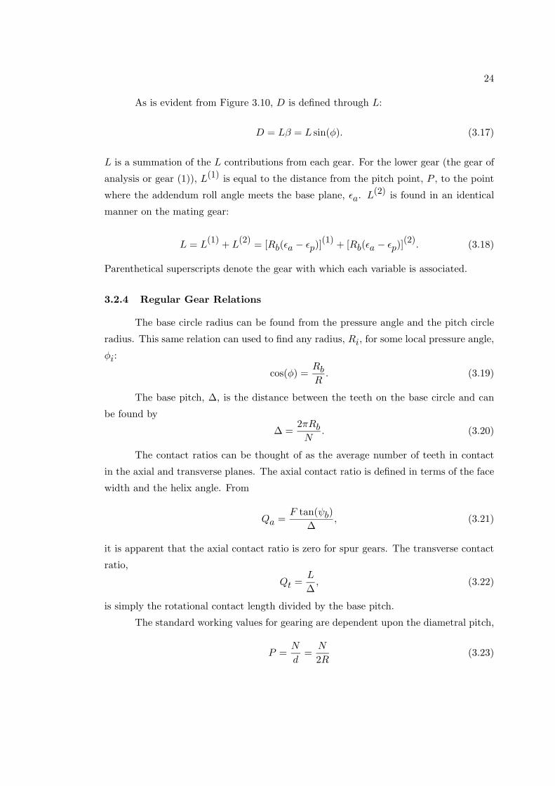
24

As is evident from Figure 3.10, D is defined through L:

D = Lβ = L sin(φ). (3.17)

L is a summation of the L contributions from each gear. For the lower gear (the gear of

analysis or gear (1)), L(1) is equal to the distance from the pitch point, P , to the point

where the addendum roll angle meets the base plane, εa. L(2) is found in an identical

manner on the mating gear:

L = L(1) + L(2) = [Rb(εa − εp)](1) + [Rb(εa − εp)](2). (3.18)

Parenthetical superscripts denote the gear with which each variable is associated.

3.2.4 Regular Gear Relations

The base circle radius can be found from the pressure angle and the pitch circle

radius. This same relation can used to find any radius, Ri, for some local pressure angle,

φi:

cos(φ) =RbR

. (3.19)

The base pitch, ∆, is the distance between the teeth on the base circle and can

be found by

∆ =2πRb

N. (3.20)

The contact ratios can be thought of as the average number of teeth in contact

in the axial and transverse planes. The axial contact ratio is defined in terms of the face

width and the helix angle. From

Qa =F tan(ψb)

∆, (3.21)

it is apparent that the axial contact ratio is zero for spur gears. The transverse contact

ratio,

Qt =L

∆, (3.22)

is simply the rotational contact length divided by the base pitch.

The standard working values for gearing are dependent upon the diametral pitch,

P =N

d=

N

2R(3.23)

25

and the circular pitch,

p =π

P. (3.24)

R is the pitch circle radius and d is the pitch circle diameter. The diametral pitch, P ,

defines the addendum radius,

Ra = R + 1/P, (3.25)

and dedendum radius,

Rd = R − 1.25/P, (3.26)

in standard American Gear Manufacturers Association proportions. These radii are the

outer most radius of the gear and inner radius located between the teeth [52].

3.3 Transmission Error

There are two components of transmission error [5]:

ζ(x) = uj(x, y) + ηj(x, y). (3.27)

The first is due to geometric variations from perfect involute teeth, η. The second is due

to deformation as a result of tooth loading, u. ζ is the transmission error and j is tooth

number. Each of these values is a sum of components due to each of the two gears in

contact:

ζ(x) = ζ(1)(x) + ζ(2)(x), (3.28)

uj(x, y) = u(1)j (x, y) + u

(2)j (x, y), (3.29)

ηj(x, y) = η(1)j (x, y) + η

(2)j (x, y). (3.30)

The superscripts denote the gear associated with each term where (1) is the gear of

analysis and (2) is the mating gear. For u and η positive values denote “removal” of

material on the involute tooth face.

If u(x, y) is due to the load on a gear tooth, some load and some stiffness must be

brought into the analysis. Define Wj(x) as the total force transmitted by tooth pair j

as measured in the plane of contact. Given that KTj(x, y) is the local stiffness per unit

length of line of contact for tooth pair j, a relation of u can be developed by

Wj(x) =

∫

LOCKTj(x, y)uj(x, y)dl. (3.31)

26

dl is the differential portion of the line of contact and is measured in the base plane.

This differential length can be related to our orthogonal coordinates by

l = y sec ψb ∴ dl = sec(ψb)dy. (3.32)

By inserting the transmission error into the force equation and rearranging, the

transmission error in terms of loading and geometric deviations from involute can be

found [5]:

Wj(x) =

∫

LOCKTj(x, y)

(ζ(x) − ηj(x, y)

)dl, (3.33)

Wj(x) = sec ψb

yB∫

yA

KTj(x, y)(ζ(x) − ηj(x, y)

)dy, (3.34)

KTj(x) = sec ψb

yB∫

yA

KTj(x, y)dy, (3.35)

ηKj(x) = sec ψb

yB∫

yA

KTj(x, y)ηj(x, y)dy, (3.36)

W (x) =∑

j

Wj(x) = ζ(x)∑

j

KTj(x) −∑

j

ηKj(x), ∴ (3.37)

η(x) =W∑

j KTj(x)+

∑j ηKj(x)

∑j KTj(x)

. (3.38)

The subscripts A and B denote the analysis endpoints on the line of contact.

3.4 The Tooth Force Equation

A very accurate method for determining the gear tooth local stiffness is developed

in detail by Alulis [51]. The gear tooth stiffness (or its inverse: the compliance) must

take into account both the global deformation including tooth cantilever deflection and

the local contact deformation. The following (Equations 3.39 through 3.50) summarizes

those techniques [5]. Each integral below is bounded by the portion of the line of contact

contained in the region of contact of the tooth face.

27

The total force transmitted by tooth pair j,

Wj(x) =

∫p′j(l, x)dl, (3.39)

can be treated as a function of the lineal force density, p′, over the line of contact.

The deformation of the tooth can be calculated from this force per unit length

along the line of contact through a compliance influence function that includes bending,

shear, and Hertzian effects:

u′j(l, x) =

∫kj(l, l

′; x)p′j(l′, x)dl′, (3.40)

where

u′j(l, x) = u′

j(y sec ψb, x) = uj(y, x). (3.41)

kj(l, l′; x) is defined as the deformation at l on the line of contact on tooth pair j

due to a unit force applied at point l′. l and l′ are reciprocal due to Maxwell’s Reciprocal

theorem [5]. Equation 3.40 is a representation of the Fredholm integral equation, and

the kernel notation used there is typical of integral equation usage. This equation can

be inverted to solve for the lineal force density,

pj(l, x) =

∫k−1j

(l, l′; x)u′j(l′, x)dl′. (3.42)

k−1j

(l, l′; x) is the stiffness influence function where the whole tooth local stiffness

is given by Equation 3.43.

K′Tj

(l, x) =

∫k−1j

(l, l′; x)dl′, (3.43)

where

K′Tj

(l, x) = K′Tj

(y sec ψb, x) = KTj(y, x). (3.44)

The tooth force equation,

Wj(x) =

∫ ∫k−1j

(l, l′; x)u′j(l, x)dl′dl, (3.45)

is developed in terms of the tooth stiffness and can be expressed as

Wj(x) =

∫K′

Tj(l, x)u′

j(l, x)dl. (3.46)

28

In the familiar x and y terms the force equation is

Wj(x) = sec ψb

∫KTj(y, x)uj(y, x)dy. (3.47)

It now becomes critical to calculate the tooth stiffness. One must adjust the

inverse Fredholm integral equation for deformation under load (Equation 3.42) for a

constant deformation. This defines the load under constant deformation:

pj(y, x) =

∫k−1j

(l, l′; x)uj(x)dl′. (3.48)

Using Equation 3.43 and solving gives the stiffness formulation,

pj(y, x)

uj(x)=

∫k−1j

(l, l′; x)dl′, (3.49)

where the full stiffness reduction becomes

KTj(y, x) =pj(y, x)

uj(x). (3.50)

As a practical matter, this representation of KTj is computed by linear algebra

for a series expansion of the loading and the lineal force density. Any function can be

represented as a series summation of orthogonal functions, and Legendre polynomials,

Pn(x) =1

2nn!

dn

dxn

(x2 − 1

)n, (3.51)

are one such family of orthogonal functions.

Modified Legendre polynomials are more appropriate for this formulation and are

defined by

Qn(x) =√

2n + 1Pn(x) =

√2n + 1

2nn!

dn

dxn

(x2 − 1

)n. (3.52)

The expansion for any function of x in modified Legendre polynomials is expressed

by

f(x) =∞∑

n=0

anQn(x) (3.53)

where

an(x) =1

2

1∫

−1

f(x)Qn(x)dx. (3.54)

29

Expressed as a matrix equation, Equation 3.40 becomes

[an]D = [C] [an]L (3.55)

where each element along the line of loading in the finite element model generates three

modified Legendre coefficients. The subscript D denotes displacement and the subscript

L denotes loading.

In Equation 3.55 the displacement vector is the result of the loading vector acting

on the compliance matrix. Each term in the compliance matrix can be found through

applying the individual loading terms to the finite element representation of the gear

tooth, finding the resultant displacement and solving for the individual compliance terms.

See Alulis [51] for a detailed explanation. The full matrices are

a0,1

a1,1

a2,1

a0,2

a1,2

a2,2

a0,3...

D

=

c11 c12 c13 c14 c15 . . .

c21 c22 c23 c24 c25 . . .

c31 c32 c33 c34 c35 . . .

c41 c42 c43 c44 c45 . . .

c51 c52 c53 c54 c55 . . ....

......

......

. . .

a0,1

a1,1

a2,1

a0,2

a1,2

a2,2

a0,3...

L

(3.56)

where in ap,e the first subscript is the polynomial order and the second subscript is the

element number along the line of contact.

Upon the completion of the full compliance matrix, a displacement can be found

for any loading or a loading can be found for a displacement. This allows for the com-

pletion of the calculation of the tooth loading force equation 3.47 or the transmission

error equation 3.38.

30

Chapter 4

The Main Procedure

4.1 Bounding the Problem

It has been established in previous chapters that the transmission error is the

exciter function for vibration and noise in meshing gears. It follows that the reduction of

transmission error is necessary in the minimization of noise. To eliminate transmission

error, the velocities and forces in a meshing gear pair must be constant throughout the

meshing of the gear pair. The zero transmission error requirement necessitates that for

a constant load a constant rotational velocity will result. Likewise, a constant load must

be transmitted in a meshing gear pair to eliminate the transmission error fluctuations.

Fourier analysis becomes important in dealing with transmission error because

it is useful to deal with the transmission error in the frequency domain. Fourier stated

that it is equivalent to describe a time-based function as a sum of frequency components.

The Fourier transform,

X(f) =

∞∫

−∞x(t)e−i2πftdt, (4.1)

allows a function to be analyzed in the frequency domain and to move back and forth

to the time domain with its inverse,

x(t) =

∞∫

−∞X(f)ei2πftdf. (4.2)

It is standard notation to denote Fourier frequency domain representations with capitol

letters and time domain function with lowercase letters.

For the computational methods included here, the discrete Fourier transform is

more appropriate:

Xn =1

N

N−1∑

k=0

xke−i2πkn/N ; n = 0, . . . , N − 1. (4.3)

31

The discrete Fourier transform also has an inverse:

xk =N−1∑

n=0

Xnei2πkn/N ; k = 0, . . . , N − 1. (4.4)

The complex Fourier series of the transmission error represents the behavior of

gear noise. The fundamental tooth-meshing harmonic frequency of n is 1/∆ meaning

that there is one Fourier coefficient per harmonic of tooth-to-tooth contact (Figure 4.1).

This is shown by

αn =1

∆

∆/2∫

−∆/2

ζ(s)e−i2πns/∆ds. (4.5)

The Fourier Uncertainty Principle becomes important in our ability to limit the

transmission error of a gear system. The Uncertainty Principle is most famous for

describing the inability to know both the location and velocity of an electron at the

same time. This idea has a counterpart in Fourier analysis. The more localized or

shorter in duration a function of time is, the more broad its frequency distribution.

Similarly, the more tightly the frequency components of a signal are clustered, the more

broad the temporal profile. There is a tradeoff between the compaction of the temporal

and frequency components of a function. Kammler [55] bounds the uncertainty with

∆s∆t ≥ 1

4π. (4.6)

This bears on the reduction of noise in gears in that for a function of finite duration

there can be no “zeroing” of the frequency components for all frequencies. For gears,

each tooth is in contact for a finite duration, therefore, the Uncertainty Principle directly

applies. However, one can eliminate the frequency component for a single frequency or

integer series of frequencies, e.g. f, 2f, 3f , etc. To minimize the noise in gears we

“zero” the harmonics of the tooth meshing fundamental (the frequency of tooth-to-tooth

contact) while maximizing the falloff of the remaining frequency components. Side bands

of the tooth meshing harmonics, which are caused by shaft rate imbalances, shaft rate

misalignment, etc., are minimized as well as these are also multiples of the tooth meshing

fundamental.

32

0 20 40 60 80 1001e−008

1e−007

1e−006

1e−005

0.0001

Fourier Transmission Error Spectrum

Gear Rotational Harmonic, n

Fou

rier

Mag

nitu

de (

mm

)

Fig. 4.1. Frequency domain theoretical gear noise is bound to integer multiples of theprimary gear rotational harmonic (n = 1). A vast majority of the noise power in realworld gears is found here as well.

4.2 The Role of Convolution in Gear Noise

Gear noise is mostly concentrated in the harmonics of the tooth meshing funda-

mental. The period of the fundamental is that of the adjacent tooth spacing, and to

illustrate this characteristic, a square function is used (Figure 4.2). The Fourier trans-

form of a square function is a continuous function with periodic zeros (or nulls). By

scaling the time domain transmission error so that the tooth meshing harmonics line up

with the zeros, a square wave type transmission error reduces the noise produced by the

gear substantially.

This central point should be emphasized. The total gear mesh force (and thereby

the transmission error) is designed in such a way that in the frequency spectrum, the

33

zeros in the force function directly overlap the tooth mesh harmonics and nullify the

primary component of gear noise. Subsequently, this technique shall be referred to as

the Fourier Null Matching technique.

0 1 2 3 4

0

0.2

0.4

0.6

0.8

1

(a)

x

h(x)

0 1 2 3 4

0

0.2

0.4

0.6

0.8

1

(c)

xh(x

)

0 5 10 15 20 25

10−4

10−3

10−2

10−1

100

(b)

f

H(ω)

0 5 10 15 20 25

10−4

10−3

10−2

10−1

100

(d)

f

H(ω)

Fig. 4.2. A unit square function (a) has a frequency spectrum (b) with zeros at integerharmonics. A unit triangle function (c) which is the convolution of two square functionsalso has a frequency spectrum (d) with zeros at the same integer harmonics. Note thedifference in the falloff of the two spectra.

A property of convolution that is utilized here states that given a function with

zeros in its Fourier transform, any convolution of that function also has zeros at the

same locations. It is established that the square function has zeros at integer frequency

34

values. The triangle function, which is the self convolution of a square function, also has

zeros at integer frequency values of its Fourier transform. A chain of convolutions can

create a continually changing profile in the time domain while the zeros of the frequency

domain are maintained. See Figure 4.3. The integral definition of convolution is

f3(s) =

∫f1(x)f2(s − x)dx. (4.7)

0 0.5 1 1.5 2 2.5 3 3.5 4

0

0.2

0.4

0.6

0.8

1

(a)

x

h(x)

0 0.5 1 1.5 2 2.5 3 3.5 4

0

0.2

0.4

0.6

0.8

1

(b)

x

h(x)

Fig. 4.3. A narrow square function is convolved with a triangle function to create anew rounded triangular function.

35

The second phase of effective noise reduction requires maximizing the falloff of the

non-integer frequency values for increasing frequency. Figure 4.4 illustrates the rate of

falloff of the Fourier transform as a function of the order of the convolution. For example,

a unit square function of width 10 convolved with a unit square function of width 2 will

result in Figure 4.4.a. This “second order” function results in a Fourier transform that

falls off as 1/f2. If Figure 4.4.a is convolved again by a unit square function of unit

width, Figure 4.4.c is the result. This “third order” function has a Fourier transform

that falls off as 1/f3.

100

102

10−5

100

frequency

(b)

100

102

10−5

100

frequency

(d)

0 1 2 3 4 5 6 7 8 9 10111213141516

0

0.2

0.4

0.6

0.8

1

(c)

x

h(x)

0 5 10 15

0

0.2

0.4

0.6

0.8

1

(a)

x

h(x)

H(f)f −1

f −2

f −3

H(f)f −1

f −2

f −3

Fig. 4.4. The convolution of two square functions can produce a triangle function or atrapezoidal function (a). Either is a “second order” function that has a Fourier transform

with asymptotic falloff of f−2 in frequency (b). A “third order” convolved function (c)

will produce a Fourier asymptotic falloff on the order of f−3 (d).

36

4.3 Convolution’s Relation to Gear Geometry

0 ∋ −∆ 0 ∆

0

Α1

Α2

(a)

s

f(s)

−∆− /2∋ −∆+ /2∋ − /2∋ 0 /2∋ ∆− /2∋ ∆+ /2∋

0

Α

(b)

s

f(s)

Fig. 4.5. A square function of width ε convolves with a triangular function of width 2∆to form a new function with a third order Fourier asymptotic falloff.

Given a triangle function, the convolution of a smaller square function produces

a rounded triangle of width 2∆ + ε as can be seen in Figure 4.5. The Fourier transform

of this function has zeros on integer multiples of 1/∆ and integer multiples of 1/ε. If

37

the triangle function represents the stiffness of a gear tooth and ∆ is the tooth spacing,

there are zeros on each of the tooth harmonics.

The curved triangle in Figure 4.5.b can be represented by a set of 5 equations

(4.8a-4.8e), where A = A1A2:

f1(s) =A

2∆(ε/2 + ∆ + s)2 , −∆ − ε/2 ≤ s ≤ −∆ + ε/2; (4.8a)

f2(s) =Aε

∆(∆ + s) , −∆ + ε/2 ≤ s ≤ −ε/2; (4.8b)

f3(s) = A

(−1

∆

(ε2/4 + s2

)+ ε

), −ε/2 ≤ s ≤ ε/2; (4.8c)

f4(s) =Aε

∆(∆ − s) , ε/2 ≤ s ≤ ∆ − ε/2; (4.8d)

f5(s) =A

2∆(ε/2 + ∆ − s)2 , ∆ − ε/2 ≤ s ≤ ∆ + ε/2. (4.8e)

4.4 Developing the Procedure

Equations 4.8 can be linked to gear tooth parameters by the following relations:

ε = ∆αu′

H(4.9)

and

A =HΩ

∆

1 + β

(αu′

H

)1+k (4.10)

Here α is the force weighting factor, β is the load weighting factor, and k is the load slope

factor. They are assumed to be 1, 32/63, and 1/4 respectively. α allows for applying the

process to a loading scale that is less that the full design loading for the gear. β and k are

chosen to ensure that the gear tooth geometry behaves in a manufacturable way. u′ is the

tooth surface deformation and H is the maximum tooth surface deformation (assumed

to be 25 µm which is approximately the deformation experienced by fully loaded steel

gears). ∆ is the base pitch as described in Equation 3.20. Ω is defined as the force per

unit depth tooth surface deflection over a line of contact.

38

Assuming the loading function, Wj(s), from Equations 3.47 is equal to f(s) in

Equation 4.8c, the case where s = 0 yields a simple relation:

Wj(0) = αΩu′(

1 − αu′

4H

)1 + β

(αu′

H

)1+k . (4.11)

The more general case of the tooth loading function for any s can be found by

combining Equations 4.8 through 4.10:

Wj(s) =ΩH

2

1 + β

(αu′

H

)1+k

(1 +

α

2

u′

H+

s

∆

)2

, (4.12a)

(−1 − α

2

u′

H

)≤ s

∆≤

(−1 +

α

2

u′

H

);

Wj(s) = αΩu′1 + β

(αu′

H

)1+k

(1 +

s

∆

), (4.12b)

(−1 +

α

2

u′

H

)≤ s

∆≤

(−α

2

u′

H

);

Wj(s) = ΩH

1 + β

(αu′

H

)1+k

αu′

H− 1

4

(αu′

H

)2

−( s

∆

)2

, (4.12c)

(−α

2

u′

H

)≤ s

∆≤

(α

2

u′

H

);

Wj(s) = αΩu′1 + β

(αu′

H

)1+k

(1 − s

∆

), (4.12d)

(α

2

u′

H

)≤ s

∆≤

(1 − α

2

u′

H

);

Wj(s) =ΩH

2

1 + β

(αu′

H

)1+k

(1 +

α

2

u′

H− s

∆

)2

, (4.12e)

(1 − α

2

u′

H

)≤ s

∆≤

(1 +

α

2

u′

H

).

It is important to note that the tooth loading is a symmetric function, i.e. Wj(s) =

Wj(−s). Equation set 4.12 gives a relation for the total applied load for a given line of

39

contact at a given surface deflection. The overall approach is to determine modifications

(material removal) from tooth surfaces that will provide constant transmitted loading, as

described above, and zero transmission error fluctuations (constant u′ for any prescribed

loading).

4.5 Applying Fourier Principles

At low loading levels, nominally perfect, rigid helical gears would possess a rect-

angular contact region. This ideal contact region could cover the majority of the tooth

surface or could be a smaller portion of the available area due to tooth geometry modi-

fications such as crowning. Also, as a rough approximation, the load transmitted across

the gear mesh for given surface deflection is proportional to the width of the line of

contact. Therefore, as the gear of analysis rotates, the load function (or alternately, the

load carrying capacity for a given line of contact) behaves in a manner that is nearly

proportional to the length of the line of contact.

If the axial and transverse contact ratios (Equations 3.21 and 3.22) are equal, the

s = 0 line of contact intersects the corners of this rectangular region for helical gears.

This is demonstrated in Figure 4.6. This configuration translates to the “triangular”

loading function shown in Figure 4.2.c. As a practical matter, the total stiffness of the

gear surface modifies this ideal contact region and the correct contact region must be

found.

Assuming a Qa = Qt = 1 initial contact region, the edges of the unmodified region

must exactly match the “triangular” profile for transmitted load throughout tooth-to-

tooth contact for all teeth. The light loading value shall be assumed to be the loading that

is required for a uniform tooth deflection of 1 µm. The “triangular” profile requirement

can be found by

Wj(s) = αΩ0u′(1 −

∣∣∣ s

∆

∣∣∣)

. (4.13)

The force per unit depth can be found by

αΩ0 =

yB(0)∫

yA(0)

KTC(y, z)dl (4.14)

evaluated at s = 0.

40

−40 −30 −20 −10 0 10 20 30 40−3

−2

−1

0

1

2

3

y (mm)

z (m

m)

s = ∆s = ∆/2s = 0s = −∆/2s = −∆

0.2

0.25

0.3

0.35

0.4

∋(ra

d)

Fig. 4.6. The black box denotes the available area on a tooth surface. The grey boxdenotes the nominal Qa = Qt = 1 contact region. This region is only valid for very lightloading. As the line of contact travels from s = −∆ to s = ∆, the practical width of linewithin the grey-boxed contact region behaves like a triangular function. The tooth rootis located at small ε and the tooth tip is located at the upper bound of ε.

The solution to the initial contact region lies in determining the endpoints to the

load integral:

Wj(s) = sec(ψb)

yB(s)∫

yA(s)

KTC(y, z)u′dy. (4.15)

Note that u′0

is a constant which leads to

Wj(s) = u′0

yB(s)∫

yA(s)

KTC(y, z)dl (4.16)

where the line of contact differential is defined as dl = sec(ψb)dy.

To bound the problem further, symmetry about the contact region should be

maintained. The change from the nominal rectangular contact region should be applied

in equal quantities to both ends of the line of contact. Assuming this symmetry, setting

Equation 4.16 equal to Equation 4.13 gives the endpoint adjustment, e, for the line of

contact at any s:

e = yA0(s) − yA(s) = yB(s) − yB0(s). (4.17)

41

Here the subscript 0 denotes the nominal rectangular region.

In this manner, the “light loading” region is determined and the appropriate

adjustments are made to the nominal rectangular region.

4.6 Extending the Contact Region

For any given s, the contact region solution for “light loading” should be extended

for a range of loadings. The intuitive fact that increased loading translates to an increased

range of contact provides the mechanism for maintaining reduced transmission error

fluctuations. The character of the extended lines of contact, under increasing load, are

controlled so as to maintain the traits of the convolution foundation of the Fourier Null

Matching Technique.

4.6.1 The First Step

Applying an increased loading to a line of contact across a tooth face will increase

the width and depth of that line of contact. The load equation, Equation 4.12, must be

expanded and evaluated. For example, the expansion of Equation 4.12c begins as follows

about s = 0:

Wj(s) = αΩu′ + . . . (4.18)

This allows two loading terms to be defined, the load mean, W , and the load variation,

ΣδWj , which contains all of the remaining terms in Equation 4.18. The result is written

as

Wj(s) = W (s) + ΣδWj(s). (4.19)

The load variation can be divided into two components which are developed from

the two ends of the line of contact:

ΣδWj(s) = δWAj

(s) + δWBj

(s). (4.20)

The contributions to the load variations at each end of the line of contact,

δWj(s) =1

2KTCu′

1θ1, (4.21)

are resultant of the triangular regions at either end of the line of contact. See Figure 4.7.

42

Tooth Face Lead Position

Load

Dis

plac

emen

t

yA−θ

1y

Ay

B yB+θ

1

u′1

u′0

0

Fig. 4.7. The unmodified region of a line of contact, denoted by the flat area at loadingu′0, are extended on either side by some distance, θ1. This distance corresponds to the

first design loading, u′1.

The extension to the line of contact, θ1, must be isolated. Combining Equa-

tions 4.19 and 4.20 gives

Wj(s) − W (s) = ΣδWj(s) = δWAj

(s) + δWBj

(s). (4.22)

The equation is rearranged,

Wj(s) − αΩu′ =1

2

(KA

TC+ KB

TC

)u′1θ1, (4.23)

and θ1 is isolated:

θ1 =2

(Wj(s) − αΩu′

1

)

(KA

TC+ KB

TC

)u′1

. (4.24)

Here αΩu′1

and W (s) are evaluated over the unmodified region. KATC

and KBTC

are evaluated at the geometrical mean of the triangular end regions of the line of contact.

4.6.2 Continuing the Expansion

For each line of contact on the tooth face, the previous sections describe the

solution of determining the “light loading” or unmodified region and the first step of

43

significant loading. To expand the range of valid gear loadings, the process must be

extended for additional steps of loading. See Figure 4.8.


Load

Dis

plac

emen

t

θ2

θ1

θ1

θ2

u′2

u′1

u′0

0

Fig. 4.8. The line of contact includes two extensions beyond the unmodified contactregion. The first step extends the range by θ1 on either end and the second step extendsthe previous line length by θ2 at each end.

Subsequent loading steps can be generalized, but follow a similar form as Equa-

tion 4.24. For the generalized case, a modification to Equation 4.19 must be made. For

any i > 0, Wj(s)i+1 can be found by the following:

Wj(s)i+1 = Wj(s)i+1 + ΣδWj(s)i+1. (4.25)

Much like Equation 4.15, the load contribution of the base region must be deter-

mined for case i + 1 by

Wj(s)i+1 = sec(ψb)

∫

i+1

KTC(y, z)u′i+1

(y)dy. (4.26)

As there is no longer a uniform profile within the new load step, there is no

average load. Much as with the first load step, the load parts can be broken into the

extended regions for the new load step and the base region. Equation 4.21 must then be

44

generalized for θi+1 by

δWAj

(s) + δWBj

(s) =1

2

(KA

TC+ KB

TC

)δu′θi+1. (4.27)

θi+1 can be found by combining Equations 4.25 and 4.27 resulting in

θi+1 =2

(Wj(s)i+1 − Wj(s)i+1

)

(KA

TC+ KB

TC

)δu′

. (4.28)

Wj(s)i+1 must be evaluated over the range including θi and Wj(s)i+1 should be

evaluated over the range including θi+1. KTC should be evaluated at the endpoints of

the θi inclusive region.

4.7 Fourier Null Matching Technique

The Fourier Null Matching Technique can be summarized by reviewing the pri-

mary mechanisms of the process:

• The vast majority of transmission error arises from the tooth meshing harmonics

(Figures 4.9, 4.10).

• Tooth stiffness profiles can be created that have Fourier spectra with nulls on

integer multiples (Figure 4.11).

• These nulls can be aligned to the nominal tooth meshing harmonics (Figures 4.9,

4.11).

• The remaining gear rotational harmonics can be constrained by a decaying envelope

(Figure 4.12).

• The technique is valid over a range of loadings

The practical application of the transmission error analysis [5, 6] used in Figure 4.9

shows the predicted error spectrum. The predicted spectrum is comprised of tooth mesh-

ing harmonics. These harmonics are integer multiples of tooth-to-tooth contact events,

while measured transmission error spectra contain additional gear rotational harmonics

caused by tooth-to-tooth variations in tooth working surfaces caused by manufacturing

and installation errors [15, 14]. The Fourier Null Matching Technique holds the ana-

lytical transmission error constant while acknowledging that “real world” transmission

45

Analytical Fourier Transmission Error Spectrum

Tooth Harmonic, n

Fou

rier

Mag

nitu

de (

mm

)

0 5 10 15 20 2510−8

10−7

10−6

10−5

10−4

10−3

10−2

Fig. 4.9. An example Fourier transmission error spectrum is shown through the 25thtooth harmonic.

error contains said additional gear rotational harmonic contributions (Figure 4.10). This

should be reiterated. The analytical transmission error is constrained to be constant by

the Fourier Null Matching Technique.

46

0 5 10 15 20 2510−8

10−7

10−6

10−5

10−4

10−3

10−2 Illustrated Measured Transmission Error Spectrum

Tooth Harmonic, n

Fou

rier

Mag

nitu

de (

mm

)

Fig. 4.10. An example continuous frequency noise spectrum is illustrated where thenoise energy is centered on integer multiples of the tooth meshing fundamental.

Example Continuous FNMT Transmission Error Spectrum

Tooth Harmonic, n

Fou

rier

Mag

nitu

de (

mm

)

0 5 10 15 20 2510−8

10−7

10−6

10−5

10−4

10−3

10−2

Fig. 4.11. The frequency domain envelope of a Fourier Null Matching Technique loadprofile is shown.

47

0 5 10 15 20 2510−8

10−7

10−6

10−5

10−4

10−3

10−2 Illustrated Composite Transmission Error Spectrum

Tooth Harmonic, n

Fou

rier

Mag

nitu

de (

mm

)

Fig. 4.12. An illustration of a Fourier Null Matching Technique resultant transmissionerror spectrum is shown.

48

4.8 Practical Work Flow

The algorithms behind the Fourier Null Matching Technique are the lifeblood of

the procedure and they demonstrate how to implement the above relations to determine

a quiet gear design. See Appendix C for code and finer detail.

Each line of contact is sequenced through each uniform deformation step. Two

index loops are used. Within the primary loop, the line of contact is indexed from s = 0

to s = −∆ and then from s = 0 to s = ∆ within the Qa = Qt = 1 bounding box.

See Figures 4.6 and 4.13. The nominal step of ∆/10 is used in the primary index loop.

Inside the primary loop, the secondary loop increases the uniform deformation from a

nominal 1 µm to a full load of 25 µm.

Fig. 4.13. An illustration of several lines of contact. The outer box represents theavailable area on a tooth face. The inner box represents the Qa = Qt = 1 area whichbounds the line of contact for −∆ ≤ s ≤ ∆. The step size between lines of contact is∆/4 in s while the horizontal coordinate is y and the vertical coordinate is z.

At each line of loading, starting with s = 0, a finite element model of the gear

is created. An estimate for the initial load is made. The element sizes on the line

of contact are found from the Zero Error Cylinder Relationship [51]. The compliance

curves for each finite element within the line of contact are determined. The compliance

49

formulation is then solved and the load for the constant deformation step is determined.

Using this load the iteration is repeated until the load converges. This gives an accurate

relation for the total gear compliance at the constant deformation in that step.

Once the nominal deformation and the associated loading is determined on the

line of contact at s = 0, the value of the total force per unit deformation over the full

line of contact is determined. This value, Ω0, is the primary load capacity variable.

Continuing, the transmitted load in a gear mesh must remain constant. Therefore, Ω(s)

must maintain a triangular profile as measured in s.

Fig. 4.14. The lower triangular figure represents the force transmitted by a single toothpair as they come in and out of contact. More completely, the total force per unitdepth deformation over a line of contact as a function of s for each tooth-to-tooth cycleis represented as this triangle over the range −∆ ≤ s ≤ ∆. The upper figure is thesuperimposed transmitted forces of all tooth pairs. The total gear mesh transmittedload (sum of the superimposed triangles) remains constant as the gear rotates.

Due to the compliance of the loaded gear tooth surface, the nominal, rectangular

Qa = Qt = 1 contact region cannot remain the final contact region. The final contact

region that corresponds to the target transmitted force will aberrate from that rectangle.

The endpoints of all lines of contact must be determined according to the target Ω(s)

profile. Once all lines of contact are determined, the bounds of the final contact region

is determined and consequently, the gear geometry for that loading is determined. An

illustration is shown in Figure 4.15.

50

Fig. 4.15. A conceptual illustration of the nominal “lightly loaded” contact region(bounded in blue) that satisfies Equation 4.13. Note that the initial rectangular regionis not the bounds of the zone of contact that corresponds to a triangular transmittedforce profile. Several lines of contact are shown in red.

For the subsequent deformation steps, there is an extension of the line of contact

or contact region that is governed by Equations 4.24 or 4.28. An illustration of the first

extension loading step is shown in Figure 4.16.

In this manner, the entire sequence of deformation steps for all s for the entire

tooth face can be found, thereby determining the total tooth face geometry. This tooth

face solution possesses analytically eliminated transmission error fluctuations and loading

fluctuations. The resultant profile can be conceptualized as a either the addition of

material in the contact region, reducing region width as material is added or the removal

of material outside the contact region where more material is removed for light loading

cases and less is removed as loading and deformation are increased.

51

Fig. 4.16. A conceptual illustration of the first expanded contact region (narrow blue).The contact region that corresponds to regular transmitted force profile (e.g. a triangle)is not regularly shaped itself (e.g. not rectangular).

52

Chapter 5

The Results

5.1 Test Gear Parameters

The gear used to test the Fourier Null Matching Algorithm was determined prior

to the investigation. The parameters of the gear are shown in Table 5.1.

Table 5.1.Test Design Gear

Variable Value

Number of Teeth, N 56

Face Width, F 60.96 mm

Pitch Radius, R 83.951 mm

Pitch Cylinder Helix Angle, ψ 18

Transverse Pressure Angle, φ 17.5

Young’s Modulus, E 207 GPa

Poisson’s Ratio, ν 0.3

There are a number of commonly used, but secondary, variables associated with

the test gear. These are listed in Table 5.2 for the design gear.

53

Table 5.2.Test Design Gear Continued

Variable Value

Base Cylinder Helix Angle, ψb 17.217

Normal Pressure Angle, φn 16.692

Load Angle, θ′ 5.3318

Base Cylinder Radius, Rb 80.065 mm

Diametral Pitch, P 0.33353 mm−1

Circular Pitch, p 9.4192 mm

Outer Radius, ROD 87.398 mm

Base Pitch, ∆ 8.9829 mm

Assumed Equal Basal Range, L 17.325 mm

Available Transverse Contact Ratio, Qt 1.9286

Available Axial Contact Ratio, Qa 2.1028

Operating Tooth Depth, D 5.210 mm

54

5.2 The Test Gear

A shaded representation of the gear can be seen in Figure 5.1. The computation

of the gear compliance is performed by finite elements on a single-tooth basis (see Fig-

ures 5.2 and 5.3). The FEA model is shown in Figures 5.4 and 5.5. Figure 5.5 shows

more clearly the concentration of elements surrounding the line of contact.

Fig. 5.1. A rendered example of the test gear.

55

Fig. 5.2. A closer view of the test gear showing the pitch point, P , and point of tangency,T .

Fig. 5.3. A standard isometric view of the test gear. The pitch point, P , and point oftangency, T are indicated.

56

Fig. 5.4. An example of a finite element model used for the compliance analysis.

57

Fig. 5.5. A close up of a finite element model used for the compliance analysis. Thismodel is for s = 0.8∆

5.3 Compliance and Loading

Compliance curves are critical to the calculation of an accurate tooth surface [51].

The iterative procedure for determining the correct finite element size and a loading

profile that are self-consistent is the process that drives the extreme computational load

of the Fourier Null Matching Technique. The iterative load profiles for the 1µm displace-

ment and each of the remaining five uniform displacements (5µm - 25µm) are shown (yel-

low, magenta, teal, red, green and blue in sequence). Note the strong proportionality to

load curves indicating the progressive loading behavior of a line of contact. Normalized

curves are indistinguishable from one another and are not shown. The loading curves

are summarized below. Line of contact locations indicated in Figures 5.6 to 5.24 can be

related to their locations on the tooth surface shown in Figures 5.26 to 5.31.

Note that the key marker for viability of the loading curves for constant deforma-

tion is the buttressing effect where the curve endpoints are raised relative to the middle

of the curve. This is necessary due to the unloaded surface outside of the curve. The

raised ends are compensatory for the loading change at the end points.

58

0.0124 0.0126 0.0128 0.013 0.0132 0.0134 0.0136 0.0138

0

2000

4000

6000

8000

10000

12000

For line of contact s = −0.9∆

Axial Position (m)

Nor

mal

Loa

ding

(N

/m)

u′ = 25 µmu′ = 20 µmu′ = 15 µmu′ = 10 µmu′ = 5 µmu′ = 1 µm

Fig. 5.6. The loading curves for s = −0.008085 m

0.0105 0.011 0.0115 0.012 0.0125 0.0130

2000

4000

6000

8000

10000

12000


Axial Position (m)

Nor

mal

Loa

ding

(N

/m)



59

0.0085 0.009 0.0095 0.01 0.0105 0.011 0.0115 0.012

2000

4000

6000

8000

10000

12000


Axial Position (m)

Nor

mal

Loa

ding

(N

/m)



0.0065 0.007 0.0075 0.008 0.0085 0.009 0.0095 0.01 0.0105 0.011

2000

4000

6000

8000

10000

12000


Axial Position (m)

Nor

mal

Loa

ding

(N

/m)



60

0.005 0.006 0.007 0.008 0.009 0.01

2000

4000

6000

8000

10000

12000


Axial Position (m)

Nor

mal

Loa

ding

(N

/m)



0.003 0.004 0.005 0.006 0.007 0.008 0.009

2000

4000

6000

8000

10000

12000


Axial Position (m)

Nor

mal

Loa

ding

(N

/m)



61

0 0.002 0.004 0.006 0.008 0.01

1000

2000

3000

4000

5000

6000

7000

8000


Axial Position (m)

Nor

mal

Loa

ding

(N

/m)



−0.005 0 0.005 0.01

1000

2000

3000

4000

5000

6000


Axial Position (m)

Nor

mal

Loa

ding

(N

/m)



62

−0.01 −0.005 0 0.005 0.01

500

1000

1500

2000

2500

3000

3500

4000


Axial Position (m)

Nor

mal

Loa

ding

(N

/m)



−0.01 −0.005 0 0.005 0.01

500

1000

1500

2000

2500

3000

3500

4000

For line of contact s = 0

Axial Position (m)

Nor

mal

Loa

ding

(N

/m)


Fig. 5.15. The loading curves for s = 0 m

63

−0.01 −0.005 0 0.005 0.01

500

1000

1500

2000

2500

3000

3500

4000

For line of contact s = 0.1∆

Axial Position (m)

Nor

mal

Loa

ding

(N

/m)


Fig. 5.16. The loading curves for s = 0.00089833 m

−0.012 −0.01 −0.008 −0.006 −0.004 −0.002 0 0.002 0.004 0.006

500

1000

1500

2000

2500

3000

3500

4000

4500

5000


Axial Position (m)

Nor

mal

Loa

ding

(N

/m)



64

−0.012 −0.01 −0.008 −0.006 −0.004 −0.002 0 0.002

1000

2000

3000

4000

5000

6000


Axial Position (m)

Nor

mal

Loa

ding

(N

/m)



−0.011 −0.01 −0.009−0.008−0.007−0.006−0.005−0.004−0.003−0.002−0.001

1000

2000

3000

4000

5000

6000

7000

8000


Axial Position (m)

Nor

mal

Loa

ding

(N

/m)



65

−0.01 −0.009 −0.008 −0.007 −0.006 −0.005

1000

2000

3000

4000

5000

6000

7000

8000

9000

10000

11000


Axial Position (m)

Nor

mal

Loa

ding

(N

/m)



−0.011−0.0105 −0.01 −0.0095−0.009−0.0085−0.008−0.0075−0.007−0.0065

1000

2000

3000

4000

5000

6000

7000

8000

9000

10000

11000


Axial Position (m)

Nor

mal

Loa

ding

(N

/m)



66

−0.012 −0.0115 −0.011 −0.0105 −0.01 −0.0095 −0.009 −0.0085

1000

2000

3000

4000

5000

6000

7000

8000

9000

10000


Axial Position (m)

Nor

mal

Loa

ding

(N

/m)



−0.013 −0.0125 −0.012 −0.0115 −0.011 −0.0105 −0.01

1000

2000

3000

4000

5000

6000

7000

8000

9000

10000


Axial Position (m)

Nor

mal

Loa

ding

(N

/m)



67

−0.014 −0.0138−0.0136−0.0134−0.0132 −0.013 −0.0128−0.0126−0.0124−0.0122

0

1000

2000

3000

4000

5000

6000

7000

8000

9000

10000


Axial Position (m)

Nor

mal

Loa

ding

(N

/m)



The total force per unit deflection, αΩ, from the loading profiles is shown in

Table 5.3. The total loading and torque can be found from the average radius of the line

of contact and the deformation as shown in Equation 5.1.

τ = WR = αΩuR (5.1)

68

Table 5.3.Summary of αΩ(N/µm).

s u = 1 µm u = 5 µm u = 10 µm u = 15 µm u = 20 µm u = 25 µm

−0.9∆ 0.2392 0.2332 0.2421 0.2426 0.2437 0.2443

−0.8∆ 0.4784 0.4843 0.5006 0.4908 0.5094 0.5144

−0.7∆ 0.7176 0.713 0.714 0.717 0.7198 0.7226

−0.6∆ 0.9568 0.9532 0.9539 0.9573 0.9602 0.963

−0.5∆ 1.196 1.206 1.211 1.21 1.214 1.217

−0.4∆ 1.435 1.436 1.453 1.455 1.462 1.467

−0.3∆ 1.674 1.672 1.672 1.674 1.676 1.677

−0.2∆ 1.914 1.912 1.912 1.916 1.913 1.914

−0.1∆ 2.153 2.152 2.154 2.116 2.092 2.152

0.0 2.392 2.391 2.357 2.336 2.317 2.303

0.1∆ 2.153 2.154 2.15 2.097 2.156 2.158

0.2∆ 1.914 1.92 1.92 1.921 1.922 1.923

0.3∆ 1.674 1.676 1.677 1.679 1.682 1.684

0.4∆ 1.435 1.433 1.433 1.434 1.435 1.437

0.5∆ 1.196 1.197 1.206 1.212 1.217 1.224

0.6∆ 0.9568 0.9518 0.9588 0.964 0.968 0.9748

0.7∆ 0.7176 0.7071 0.7126 0.7167 0.72 0.7262

0.8∆ 0.4784 0.4788 0.4828 0.4858 0.4882 0.4923

0.8∆ 0.2392 0.2399 0.2424 0.2441 0.2458 0.2492

69

For each deformation step, the total force per unit deflection should maintain a

nearly triangular profile. These profiles are shown normalized in Figure 5.25.

−1 −0.8 −0.6 −0.4 −0.2 0 0.2 0.4 0.6 0.8 10

0.1

0.2

0.3

0.4

0.5

0.6

0.7

0.8

0.9

1

s/∆

Nor

mal

ized

αΩ

(s)


Fig. 5.25. The nominal loading case results in a perfect triangle. The remaining loadsteps deviate slightly from a triangular profile. Note that the rounded triangle is notimmediately apparent due to resolution in s.

70

5.4 Contact Region

Each of the loading curves in Figures 5.6 - 5.24 is for a specific line of loading.

Each line of loading is bounded by the Fourier Null Matching Technique. Figures 5.26

- 5.31 show the solution lines of contact for the test gear tooth. The endpoints of each

line of contact are shown in Table 5.4.

−0.015 −0.01 −0.005 0 0.005 0.01 0.015−1.5

−1

−0.5

0

0.5

1

1.5

x 10−3 u = 1e−006 m

y (m)

z (m

)

s = −0.9∆

s = −0.8∆

s = −0.7∆

s = −0.6∆

s = −0.5∆

s = −0.4∆

s = −0.3∆

s = −0.2∆

s = −0.1∆

s = 0

s = 0.1∆

s = 0.2∆

s = 0.3∆

s = 0.4∆

s = 0.5∆

s = 0.6∆

s = 0.7∆

s = 0.8∆

s = 0.9∆

Fig. 5.26. The bounds of each line of contact and its position on the tooth face is shownin the same orientation as Figure 4.6 for deformation step u = 1µm. Blue box denotesQa = Qt = 1. The lines of contact vary from s = −0.9∆ on the lower right to s = 0.9∆on the upper left with a step between of ∆s = ∆/10. The tip of the tooth is positive zand the root is negative z.

71

−0.015 −0.01 −0.005 0 0.005 0.01 0.015−1.5

−1

−0.5

0

0.5

1

1.5

x 10−3 u = 5e−006 m

y (m)

z (m

)

s = −0.9∆

s = −0.8∆

s = −0.7∆

s = −0.6∆

s = −0.5∆

s = −0.4∆

s = −0.3∆

s = −0.2∆

s = −0.1∆

s = 0

s = 0.1∆

s = 0.2∆

s = 0.3∆

s = 0.4∆

s = 0.5∆

s = 0.6∆

s = 0.7∆

s = 0.8∆

s = 0.9∆

Fig. 5.27. The bounds of each line of contact for deformation step u = 5µm. Blue boxdenotes Qa = Qt = 1. The lines of contact vary from s = −0.9∆ on the lower right tos = 0.9∆ on the upper left with a step between of ∆s = ∆/10. The tip of the tooth ispositive z and the root is negative z.

72

−0.015 −0.01 −0.005 0 0.005 0.01 0.015−1.5

−1

−0.5

0

0.5

1

1.5

x 10−3 u = 1e−005 m

y (m)

z (m

)

s = −0.9∆

s = −0.8∆

s = −0.7∆

s = −0.6∆

s = −0.5∆

s = −0.4∆

s = −0.3∆

s = −0.2∆

s = −0.1∆

s = 0

s = 0.1∆

s = 0.2∆

s = 0.3∆

s = 0.4∆

s = 0.5∆

s = 0.6∆

s = 0.7∆

s = 0.8∆

s = 0.9∆


73

−0.015 −0.01 −0.005 0 0.005 0.01 0.015−1.5

−1

−0.5

0

0.5

1

1.5

x 10−3 u = 1.5e−005 m

y (m)

z (m

)

s = −0.9∆

s = −0.8∆

s = −0.7∆

s = −0.6∆

s = −0.5∆

s = −0.4∆

s = −0.3∆

s = −0.2∆

s = −0.1∆

s = 0

s = 0.1∆

s = 0.2∆

s = 0.3∆

s = 0.4∆

s = 0.5∆

s = 0.6∆

s = 0.7∆

s = 0.8∆

s = 0.9∆


74

−0.015 −0.01 −0.005 0 0.005 0.01 0.015−1.5

−1

−0.5

0

0.5

1

1.5

x 10−3 u = 2e−005 m

y (m)

z (m

)

s = −0.9∆

s = −0.8∆

s = −0.7∆

s = −0.6∆

s = −0.5∆

s = −0.4∆

s = −0.3∆

s = −0.2∆

s = −0.1∆

s = 0

s = 0.1∆

s = 0.2∆

s = 0.3∆

s = 0.4∆

s = 0.5∆

s = 0.6∆

s = 0.7∆

s = 0.8∆

s = 0.9∆


75

−0.015 −0.01 −0.005 0 0.005 0.01 0.015−1.5

−1

−0.5

0

0.5

1

1.5

x 10−3 u = 2.5e−005 m

y (m)

z (m

)

s = −0.9∆

s = −0.8∆

s = −0.7∆

s = −0.6∆

s = −0.5∆

s = −0.4∆

s = −0.3∆

s = −0.2∆

s = −0.1∆

s = 0

s = 0.1∆

s = 0.2∆

s = 0.3∆

s = 0.4∆

s = 0.5∆

s = 0.6∆

s = 0.7∆

s = 0.8∆

s = 0.9∆


76

−0.015 −0.01 −0.005 0 0.005 0.01 0.015

−1.5

−1

−0.5

0

0.5

1

1.5

x 10−3 Contact Region at Each Deformation Step

y (m)

z (m

)

1µm5µm10µm15µm20µm25µm

Fig. 5.32. The estimated contact region for the final geometry is seen. Note the well-behaved portion of the tooth: negative s (lower right) for deformation steps from 5 µmto 25 µm.

77

Table 5.4.Summary of Line of Contact End Points. All values in m.

u = 1µm u = 5µm u = 10µm u = 15µm u = 20µm u = 25µm

s yBlower yBupper yBlower yBupper yBlower yBupper yBlower yBupper yBlower yBupper yBlower yBupper

-0.9∆ 0.012228 0.013863 0.012858 0.013233 0.012587 0.013504 0.012516 0.013574 0.012482 0.013609 0.012453 0.013637

-0.8∆ 0.010183 0.013008 0.011318 0.011873 0.010833 0.012359 0.010725 0.012467 0.010644 0.012548 0.010582 0.012609

-0.7∆ 0.0082266 0.012066 0.0099311 0.010362 0.0090778 0.011215 0.0088743 0.011418 0.0087872 0.011505 0.0087066 0.011586

-0.6∆ 0.0063243 0.011069 0.0081266 0.0092671 0.007199 0.010195 0.0069598 0.010434 0.0068595 0.010534 0.0067722 0.010621

-0.5∆ 0.0044272 0.010068 0.0060372 0.0084575 0.0052184 0.0092763 0.0049811 0.0095136 0.0048609 0.0096338 0.0047606 0.0097341

-0.4∆ 0.002596 0.0089998 0.0039457 0.0076501 0.0032398 0.008356 0.0030022 0.0085936 0.0028634 0.0087324 0.0027639 0.0088319

-0.3∆ -0.0015303 0.010227 -0.00002171 0.0087186 -0.0008551 0.0095519 -0.0011994 0.0098962 -0.0013931 0.01009 -0.0015084 0.010205

-0.2∆ -0.0057305 0.011528 -0.0044075 0.010205 -0.0052502 0.011048 -0.0056204 0.011418 -0.005886 0.011684 -0.0060804 0.011878

-0.1∆ -0.011914 0.014813 -0.011434 0.014333 -0.011892 0.014791 -0.012193 0.015092 -0.012415 0.015314 -0.012698 0.015597

0 -0.014495 0.014495 -0.014683 0.014683 -0.014765 0.014765 -0.014967 0.014967 -0.015175 0.015175 -0.015352 0.015352

0.1∆ -0.014998 0.0121 -0.014534 0.011635 -0.014982 0.012083 -0.015275 0.012376 -0.0156 0.012701 -0.015791 0.012892

0.2∆ -0.013797 0.0079994 -0.016132 0.010334 -0.014065 0.0082667 -0.013809 0.0080106 -0.014008 0.0082102 -0.014212 0.0084137

0.3∆ -0.012631 0.0039339 -0.014921 0.0062245 -0.014719 0.006022 -0.014975 0.0062785 -0.01279 0.004093 -0.01263 0.0039331

0.4∆ -0.011511 -0.00008526 -0.013277 0.0016815 -0.01308 0.0014844 -0.013234 0.001638 -0.011354 -0.00024167 -0.011272 -0.00032394

0.5∆ -0.010343 -0.0041521 -0.011644 -0.0028505 -0.011322 -0.0031727 -0.011365 -0.00313 -0.011523 -0.0029712 -0.011711 -0.0027835

0.6∆ -0.011356 -0.0060372 -0.012598 -0.0047956 -0.012292 -0.0051014 -0.012317 -0.0050762 -0.01245 -0.0049436 -0.013171 -0.0042229

0.7∆ -0.012315 -0.0079777 -0.013398 -0.0068946 -0.013132 -0.0071605 -0.013145 -0.0071478 -0.013894 -0.0063983 -0.013959 -0.0063334

0.8∆ -0.013253 -0.0099388 -0.014129 -0.0090624 -0.013909 -0.0092826 -0.014596 -0.0085958 -0.014625 -0.0085661 -0.014574 -0.0086177

0.9∆ -0.014033 -0.012058 -0.014524 -0.011567 -0.014908 -0.011183 -0.014887 -0.011204 -0.014813 -0.011278 -0.014766 -0.011324

78

5.5 Endpoint Modification

In each end point region of the progression of the Fourier Null Matching Tech-

nique, the variation and slope at the boundary of the contact region is the determining

factor for the utility and manufacturable of the gear as a whole. The end point solution

is the culmination of the work of Mark [5, 6] and Alulis [51] which results in a solution

for minimizing transmission error and loading variations and as a consequence, noise.

Figures 5.34 through 5.52 show the positive y side of the line of contact for each loading

set. The negative y side is identical since the problem is constrained to be symmetric

about the contact region. See the example in Figure 5.33. Each graph (and line of

contact at some s) is the solution for the full series of deformation cases at that location.


Load

Dis

plac

emen

t

θ5

θ4

θ3

θ2θ

1yA

yB

θ1θ

2θ

3θ

4θ

5

u′5

u′4

u′3

u′2

u′1

u′00

Fig. 5.33. Each line of contact is constrained to have symmetric adjustments to thelength of the line of contact for each deformation step. The positive-y extension profileis a mirror of the negative-y deformation profile.

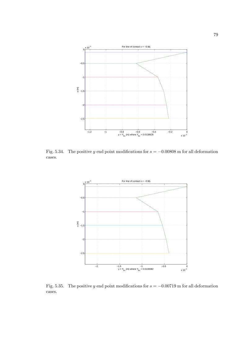
79

−1.2 −1 −0.8 −0.6 −0.4 −0.2 0

x 10−3

−2.5

−2

−1.5

−1

−0.5

0x 10

−5

y + Ybu

(m) where Ybu

= 0.0138626

u (m

)


Fig. 5.34. The positive y end point modifications for s = −0.00808 m for all deformationcases.

−2 −1.5 −1 −0.5 0

x 10−3

−2.5

−2

−1.5

−1

−0.5

0x 10

−5

y + Ybu

(m) where Ybu

= 0.0130082

u (m

)



80

−3 −2.5 −2 −1.5 −1 −0.5 0

x 10−3

−2.5

−2

−1.5

−1

−0.5

0x 10

−5

y + Ybu

(m) where Ybu

= 0.012066

u (m

)



−3.5 −3 −2.5 −2 −1.5 −1 −0.5 0

x 10−3

−2.5

−2

−1.5

−1

−0.5

0x 10

−5

y + Ybu

(m) where Ybu

= 0.0110694

u (m

)



81

−3 −2.5 −2 −1.5 −1 −0.5 0

x 10−3

−2.5

−2

−1.5

−1

−0.5

0x 10

−5

y + Ybu

(m) where Ybu

= 0.0100675

u (m

)



−2.5 −2 −1.5 −1 −0.5 0

x 10−3

−2.5

−2

−1.5

−1

−0.5

0x 10

−5

y + Ybu

(m) where Ybu

= 0.00899975

u (m

)



82

−3 −2.5 −2 −1.5 −1 −0.5 0

x 10−3

−2.5

−2

−1.5

−1

−0.5

0x 10

−5

y + Ybu

(m) where Ybu

= 0.0102272

u (m

)



−2.5 −2 −1.5 −1 −0.5 0

x 10−3

−2.5

−2

−1.5

−1

−0.5

0x 10

−5

y + Ybu

(m) where Ybu

= 0.011518

u (m

)



83

−15 −10 −5 0 5

x 10−4

−2.5

−2

−1.5

−1

−0.5

0x 10

−5

y + Ybu

(m) where Ybu

= 0.0148132

u (m

)


Fig. 5.42. The positive y end point modifications for s = −0.000898 m for all deforma-tion cases.

−8 −6 −4 −2 0 2 4 6 8

x 10−4

−2.5

−2

−1.5

−1

−0.5

0x 10

−5

y + Ybu

(m) where Ybu

= 0.0144947

u (m

)

For line of contact s = 0

Fig. 5.43. The positive y end point modifications for s = 0 m for all deformation cases.

84

−15 −10 −5 0 5

x 10−4

−2.5

−2

−1.5

−1

−0.5

0x 10

−5

y + Ybu

(m) where Ybu

= 0.012147

u (m

)


Fig. 5.44. The positive y end point modifications for s = 0.000898 m for all deformationcases.

−2 −1.5 −1 −0.5 0 0.5 1 1.5 2

x 10−3

−2.5

−2

−1.5

−1

−0.5

0x 10

−5

y + Ybu

(m) where Ybu

= 0.00803416

u (m

)



85

−2 −1.5 −1 −0.5 0 0.5 1 1.5 2

x 10−3

−2.5

−2

−1.5

−1

−0.5

0x 10

−5

y + Ybu

(m) where Ybu

= 0.00397132

u (m

)



−2 −1.5 −1 −0.5 0 0.5 1 1.5

x 10−3

−2.5

−2

−1.5

−1

−0.5

0x 10

−5

y + Ybu

(m) where Ybu

= −7.62256e−005

u (m

)



86

−1 −0.5 0 0.5 1

x 10−3

−2.5

−2

−1.5

−1

−0.5

0x 10

−5

y + Ybu

(m) where Ybu

= −0.00412936

u (m

)



−1.5 −1 −0.5 0 0.5 1 1.5

x 10−3

−2.5

−2

−1.5

−1

−0.5

0x 10

−5

y + Ybu

(m) where Ybu

= −0.00603724

u (m

)



87

−1.5 −1 −0.5 0 0.5 1 1.5

x 10−3

−2.5

−2

−1.5

−1

−0.5

0x 10

−5

y + Ybu

(m) where Ybu

= −0.00797768

u (m

)



−1 −0.5 0 0.5 1

x 10−3

−2.5

−2

−1.5

−1

−0.5

0x 10

−5

y + Ybu

(m) where Ybu

= −0.00993876

u (m

)



88

−8 −6 −4 −2 0 2 4 6 8

x 10−4

−2.5

−2

−1.5

−1

−0.5

0x 10

−5

y + Ybu

(m) where Ybu

= −0.0120567

u (m

)



89

5.6 Discussion of Computed Contact Regions

There are four key concepts that bear on the results in Figures 5.26 through 5.31.

First, the Hertzian stiffness for gear tooth contact increases with increased deformation.

Welker [49] shows these relations very succinctly in Appendix A. The Hertzian stiff-

ness is also very small for small deformations relative to total tooth stiffness. Second,

the Hertzian stiffness is proportional to the length of a line of contact to first order.

With this, the length of a line of contact can be used as a qualitative measure of the

Hertzian contribution to total stiffness. Third, the nonlinear increase in Hertzian stiff-

ness decreases with increasing deformation. Again see Welker, Appendix A. Finally, the

bending stiffness of the tooth deformations is larger near the root (negative s) and de-

creases as a line of contact travels toward the tip (positive s). Also note that the imposed

loading, as shown in Figure 5.25, is symmetric about s = 0 for each deformation case.

Figure 5.26 shows the assumed negligible loading case. This initial case demon-

strates the Hertzian stiffness behavior for small deformations. For these small deforma-

tions, the Hertzian stiffness is also small and as a result, almost all of the deformation for

this case is of the Hertzian variety. The bending stiffnesses are not operative because the

effective bending stiffnesses are much higher than Hertzian stiffnesses for light loading.

Without tooth bending or gross tooth stiffness as significant contributors to global tooth

stiffness, the computed bound lines of contact are largely symmetrical about s = 0 as a

result of the symmetrical imposed total loading.

The relative and qualitative magnitude of the bending stiffness contribution can

be seen in the differences in the negative s and positive s behavior in Figure 5.26.

The length for a given positive s line of contact is slightly longer than its negative s

counterpart. The difference in the lengths of these pairs of lines of contact is traced to

the increase in the Hertzian stiffness contribution to total stiffness that is required near

the tip of the gear tooth (positive s). In the tip region, the tooth bending stiffness is

smaller compared to that at the tooth root (negative s). Consequently, the positive s

Hertzian stiffness contribution must be larger than that of the negative s counterpart.

The length of the line of contact is therefore correspondingly longer in the positive s

portion of the tooth.

Figure 5.27 shows the lines of contact for the first deformation step that is designed

to be fully engaged. This deformation step is 5 µm. The distribution of the Hertzian and

the bending components of total stiffness has changed with respect to the nominal light

loading case shown in Figure 5.26. The applicable bending stiffness contribution to total

90

stiffness in the positive s portion of the contact region is much smaller than that in the

negative s portion. This extends the lines of contact. This effect is a result of the imposed

symmetric loading shown in Figure 5.25 and the analytical tooth behavior. Conversely,

the negative s portion of the contact region exhibits shorter lines of contact relative to

their positive counterparts. Here the Hertzian component of total stiffness is reduced,

which results in the reduced contact line lengths. It is obvious that such a reduction

relative to the nominal line of loading is not physically achievable. An increase in the

load weighting factor’s assumed value (β = 32/63) should help to address this physical

discrepancy.

Figure 5.28 shows that the subsequent deformation step to Figure 5.27 behaves

in a similar fashion. The bending stiffness portion of the total stiffness at the root (neg-

ative s) is relatively large allowing shorter lines of contact and the associated Hertzian

stiffness carry the majority of the imposed loading in this region. Since the Hertzian

component of stiffness is largely proportional to length of the line of contact the neg-

ative s contact lines are shorter by comparison. As the deformation and loading are

incrementally increased a nonlinear increase in total computed stiffness results from the

Fourier Null Matching Technique. Continuing in the negative s region, the load weight-

ing factor, β, is sufficiently large to ensure a positive increase in the length of the line

of contact as tooth deformation is increased. Figures 5.29, 5.30, and 5.31 show the

positive contact line extension for increasing deformation in the negative s region. The

load weighting factor, β, is developed to “overcome” the nonlinear increases in Hertzian

stiffness in Equations 4.12 and 4.28 in such a way that as deformation and loading are

increased the length of the line of contact is also increased.

In the positive s region, the bending stiffness is smaller than in the root region.

Hence, the Hertzian contribution to total stiffness is greater in proportion to the total

requisite stiffness as a result of the imposed loading. With this greater Hertzian com-

ponent, the length of the lines of contact in the positive s region must be greater as

well. This is clearly shown in Figures 5.28 through 5.31. The behavior of the larger

nonlinear Hertzian stiffness contribution demonstrates that the load weighting factor, β,

is not sufficiently large in these analyses to “overcome” the actual nonlinearities in the

Hertzian contribution. This is expressed as negative extension to the length of the line

of contact as deformation is increased by Equation 4.28. A value for the load weighting

factor, β, larger than the 32/63 used could have corrected this issue and the nonpractical

resultant design geometry. The positive s region demonstrates that for future analyses, a

larger load weighting factor, β, and possibly a modified load slope factor, k, is called for

91

to realize a tooth surface design that is physically feasible. The load weighting factor,

β, controls the nonlinear stiffness characteristic of the model which by Equation 4.28

controls the extension of the lengths of the lines of contact.

The analysis contained herein is for a single gear, and using the Fourier Null

Matching Technique for a practical application will require the analysis of a mating gear

pair. Careful control of the mating gear pair may allow for the joint mesh stiffness to

maintain good behavior throughout the gear rotation.

92

Chapter 6

Summary and Conclusions

6.1 The Fourier Null Matching Technique

The current state of the art in gear analysis has been expanded to create a proce-

dure for designing an optimal tooth face modification for reducing or eliminating trans-

mission error variation across a range of loadings. Despite the limitations of the positive

s contact region, the technique has shown that a rigorous gear mesh analysis protocol

can be used to design an optimal contact region for a helical gear for a given deformation.

At a given deformation step, the helical gear of analysis and its results show that

the contact region can be controlled in such a way as to create a mesh stiffness profile

that maintains a constant transmission error, maintains a constant transmitted load, and

creates operational nulls on the tooth meshing harmonics. This constitutes a significant

advance in the analytical state of the art for gearing.

It should be duly noted that the transmission error analysis that is the basis

of the Fourier Null Matching Technique is a static analysis. The transmission error

is accepted to be largely proportional to measured gear noise: implying that dynamic

effects are secondary [15, 11, 13]. Given that the transmission error is, in large part,

proportional to and the root of gear noise and vibration, the Fourier Null Matching

Technique significantly reduces the source of gear noise by eliminating the tooth meshing

harmonics of transmission error while maintaining constant transmitted load. The tooth

surface modification techniques contained herein expand the capabilities of standard gear

analysis, prediction and design.

The example computation shows that using a very accurate gear stiffness model,

it is feasible to compute the contact region on a gear tooth face that will provide a

constant transmission error and a constant mesh loading over a range of mesh loadings

and transmission errors.

93

6.2 The Practicality of the Tooth Modification

Gear grinding equipment can typically reach a geometric accuracy of approxi-

mately 1 µm [54]. With a mean step distance on the order of 0.5 mm, it is realistic

to attempt to manufacture the negative s portion of contact region for the deformation

ranges of 5 µm to 25 µm. The positive s portion of gear tooth surface is not manufac-

turable given the negative extension results. In addition, the nominal “light loading”

deformation (1 µm) does not sufficiently engage the tooth compliance to maintain the

Fourier Null Matching Technique. The first step of the analysis should be increased in

magnitude and reevaluated.

The ultimate practicality of the as-designed tooth face will likely lie in the joint

gear mesh solution’s ability to compensate for the expressed compliance behavior near

the tooth tip (positive s). Additional compromises for manufacturability, for the non-

ideal realities of installed gear sets, and for life cycle longevity may have to be made.

With the careful design of whole gear systems, the technical limitations of quiet gears

that are made apparent by the Fourier Null Matching Technique can be addressed in the

majority of powertrain applications.

The base outline of the contact region for any given deformation step is likely

to have significant applicability and noise reduction capability across a limited range of

loading levels. As a practical matter the contact regions demonstrated in Figures 5.27-

5.31 may be construed as a rough guideline for the form of the contact region that is

necessary for quiet operation. Within the limits of manufacturability, material knowl-

edge, and implementability, the Fourier Null Matching Technique has the potential to

significantly alter gear analysis, gear design and powertrain operation.

6.3 Limitations of the Analysis

The Fourier Null Matching Technique requires high precision and as such, there

are a number of limiting factors in the technique’s utility. First and foremost, the

technique is limited by the knowledge of the gear material. Lack of knowledge of grain

structure, Young’s modulus and Poisson’s ratio adds variability and uncertainty to the

full technique. Material properties are crucial to accurate finite element computation.

Hence, normal material property knowledge is limiting.

Implementing this method requires that material be removed from the tooth face.

In the case of the afore-described gear, at least 25 µm of material must be removed from

94

the tooth face outside of the contact region. The analysis gear has a pitch thickness of

approximately 4.7 mm. Removing the full design deformation amounts to a thinning of

more than 0.5%. Removing this material will modify the stiffness response of the gear

tooth and will require additional compliance iterations due to the change in physical

tooth properties, especially in the positive s region of the tooth surface.

Other factors that are present in normal gear and powertrain operation are ignored

in this analysis. Friction and lubrication properties are small and do not lay in the plane

of action of a meshing gear pair. In addition, the direction and mechanisms of friction

forces in are largely self-cancelling [14] in helical gears. Consequently, friction effects

are neglected here. However, Liu and Parker [56] have shown that the effects of friction

do express themselves in the dynamic response of the gear system. Friction should be

included in the full design of any specific installation configuration.

The final neglected situational mechanism is the structural environment of a

normal meshing gear pair. The bearings, shafts and supporting structures affect the

transmission error by introducing eccentricity and misalignment. These effects can be

accounted for systematically, but only if the magnitude of these effects are known ex-

plicitly. Sensitivity to misalignment and eccentricity should be statistically bounded for

further analysis and possible physical testing.

Shaft eccentricity affects gear noise by providing a once-per-revolution (gear rota-

tional harmonic n = 1) tooth-spacing error. Since few teeth are in contact at any given

instant, any eccentricity effect would be small.

Misalignment would affect the Fourier Null Matching Technique generated gear

much like a standard gear [57, 58]. Axially crowned gears are less affected by misalign-

ment than standard gears [59]. However, the effective contact ratio of axially crowned

gears are reduced compared to the Fourier Null Matching Technique gear or a standard

gear, and the corresponding noise properties will reflect that. As the unmodified region

maintains the involute profile without modification, misalignment will not greatly affect

vibration generation while the whole line of contact boundary is contributing to the

gear mesh. Misalignment will, however, alter the surface contact stresses. On one end

contact stresses will be increased while on the other end they will be reduced. Sufficient

misalignment for loss of contact will create additional gear noise much as a standard

gear will behave under such a scenario [58].

95

6.4 Extending the Process

This analysis is provided in a one-sided context, i.e. only the test gear is analyzed

without consideration of its mate. To the extent that complimentary gear parameters

are needed, any mating gear in the present analysis would be an ideal, rigid involute

gear of the same size as the gear of analysis. For an installed gear pair, the geometrical

compensation for the transmission error mechanisms must be applied to the gears in

tandem. Each gear must share in the surface modifications and the total gear pair mesh

stiffness must be evaluated through the Fourier Null Matching Technique.

The computation should be expanded to determine the sensitivity of the method

to the parameters β and k. Other values of these constants may lead to more gradual

slopes with respect to increasing uniform elastic deformation as noted above. This pro-

cess would require significant additional effort due to the intense computational load of

the technique. In addition, the sensitivity of the Legendre polynomial representation of

the compliance loading curves to the number and type of axial elements must be de-

termined. The dependence on the axial element configuration and number to the final

evaluation of the load integral, Equation 4.15, must be parameterized.

In using the Fourier Null Matching Technique for functional gear design, certain

modifications could be made to address other real-word issues. For example, misalign-

ment can be addressed by introducing a curvature to the gear tooth face that allows the

gear to behave similarly in both the misaligned and the correctly mounted position. In

the Fourier Null Matching Technique, the step functions used in each deformation step

could be altered to allow for curvature down the line of contact. In this manner, mis-

alignment can be addressed within the context of the Fourier Null Matching Technique.

The next conceptual step in the development of the Fourier Null Matching Tech-

nique should be to replace Alulis’ computationally intensive compliance formulation with

a more efficient model. Ideally this future compliance model will be computationally ef-

ficient enough to run statistical variations and global optimizations on the Fourier Null

Matching Technique. An elegant yet accurate relation for tooth compliance would be of

great benefit to any extension of the present analysis for the entire gear industry. With

such an advance, wide scale adoption and implementation of the Fourier Null Matching

Technique within the gear industry may ultimately be feasible.

96

6.5 Closure

The goal of this dissertation is to answer a singular question: Can a set of mod-

ifications for an involute tooth working surface be devised such that the resultant gear

will transmit a constant load and zero transmission error fluctuation for a non-negligible

range of loadings? Contained herein is a procedure that utilizes the nonlinear tooth stiff-

ness properties of a gear tooth, including all Hertzian contributions, to attempt that goal.

The results of this procedure, while being a mere first step, answer this dissertation’s

central query in the affirmative.

97

Appendix A

Notation

In gearing literature, the notation is loose and rarely self consistent. The notation

listed in Table A.1 is a compromise of the most common usage and is used throughout

this document.

Table A.1: Gearing Notation

Variable Comments

I The involute curve

ε Roll angle for any point, i, on I

εp The roll angle for the pitch point, P

ε0 The roll angle at the center of the basal range, L

φ The global pressure angle, equal to φi at i = P

φi The pressure angle for any point, i, on I

φn The normal pressure angle

θ The pitch point involute base cylinder arclength, εp − φ

θi The general involute base cylinder arclength, ε − φi

O The involute origin

T The conceptual involute tangency point

P ′ The pitch point

R The pitch circle radius

Rb The base circle radius

ψ The pitch cylinder helix angle

ψb The base cylinder helix angle

N The number of teeth on a gear

∆ The base pitch

Qa The operating axial contact ratio

Qt The operating transverse contact ratio

F The axial face width

Continued on Next Page. . .

98

Table A.1 – Continued

Variable Comments

D The operating tooth depth

L The basal tooth contact range

y The axial tooth face coordinate

z The radial tooth face coordinate

x The basal tooth coordinate

s The local basal tooth coordinate

P The diametral pitch

p The circular pitch

d The pitch diameter

β sin(φ)

γ ±β tan(ψb): positive for right hand helix

βi The angle measured from the center of the tooth to i on the involute

ιi φi − βi

θ′ The load angle of the line of contact

Rd The dedendum radius

Ra The addendum radius

εa The roll angle at the addendum

t The tooth thickness

The transmission error notation contained within this document is derived from

Mark [5]. As with all of the notation throughout this research, there are small variations

for the purpose of self-consistency. See Table A.2.

The optimization work in this thesis uses additional notation that is listed in

Table A.3.

99

Table A.2.Summary of Transmission Error Notation

Variable Comments

ζ The transmission error

u Tooth face deformation due to loading under the tooth mesh

η Tooth face variation due to geometry

j Tooth number

Table A.3.Summary of Optimization Notation

Variable Comments

A The convolution product amplitude

∆ The length of the linearly increasing portion of the convolution precursor

ε The width of the square convolution precursor

u′i

Iteration, i, of constant deflection

H The maximum design deformation (25 µm in this analysis)

Ω The force per unit depth u′ evaluated over the line of contact

α Force weighting factor (assumed to be 1)

β Load weighting factor (assumed to be 32/63)

k Load slope factor (assumed to be 1/4)

u The deflection of a gear tooth surface on a line of contact

p The lineal force density along the line of contact

kj The tooth compliance influence function

KTj The total stiffness of the gear tooth face

Wj The loading force for a given line of contact between meshing teeth

100

Appendix B

Derivations

B.1 Simplifying the Load Angle Equation

Equation 3.4 can be rearranged to the Equation B.1.

tan(θ′) =cos(φ)

cos(φn)

sin(ψ) sin(φ)

1 − sin2(ψ) sin2(φ)(B.1)

Multiplying top and bottom by cos2(ψ) cos2(φ) sin(φn) and simplifying produces

Equation B.2.

tan(θ′) =tan(ψ) tan(φ) tan(φn)

sin(φn) cos(ψ)

1

sec2(ψ) sec2(φ) − tan2(ψ) tan2(φ)(B.2)

Substituting Equation 3.3 and again multiplying top and bottom by sin(φn) fur-

ther simplifies the equality when the Pythagorean trigonometric identity is used in the

denominator.

tan(θ′) = tan(ψ) sin(φn)tan2(φ) csc2(φn)

(tan2(ψ) + 1)(tan2(φ) + 1) − tan2(ψ) tan2(φ)(B.3)

Again using the Pythagorean trigonometric identity and expanding the denomi-

nator produces Equation B.4.

tan(θ′) = tan(ψ) sin(φn)tan2(φ)(cot2(φn) + 1)

tan2(φ) + tan2(ψ) + 1(B.4)

Expanding the numerator and applying Equation 3.3 reduces the numerator. Us-

ing the Pythagorean identity a final time reduces the fraction to unity.

tan(θ′) = tan(ψ) sin(φn)tan2(φ) + sec2(ψ)

tan2(φ) + tan2(ψ) + 1(B.5)

tan(θ′) = tan(ψ) sin(φn) (B.6)

101

B.2 Radius of Curvature

Alulis’ treatment [51] of the line of contact along a tooth depends upon the ap-

plicability of the models used for determining the Zero Error Cylinder Relationship and

the actual gear. Said relationship gives an accurate finite element size given an element

depth and a Hertzian deformation width for the forces along the line of contact. The

Hertzian deformation is a function of the magnitude of the applied load and the radius

of curvature.

A relation the radius of curvature across the line of contact must be determined.

The method used to determine a relationship for the radius of curvature across the line of

contact is a brute force geometric transformation. Since the spur profile is proportional

to the roll angle and base radius, a similar correlation is assumed. Points on and about

the line of contact are mapped to global cartesian coordinates and these coordinates are

analyzed.

Any three points in cartesian space are contained within a circle of a unique

radius. The solution to the radius of a circumcircle for a triangle of three points in a

plane is shown by Weisstein [60]. The solution of the circle is shown in Equation B.7.

∣∣∣∣∣∣∣∣∣∣∣

R2 x y 1

R21

x1 y1 1

R22

x2 y2 1

R23

x3 y3 1

∣∣∣∣∣∣∣∣∣∣∣

= 0 (B.7)

Where any R2i

= x2i

+ y2i. Weisstein shows how the radius and center can be

found by using the equation of a quadratic curve.

ax2 + cy2 + dx + ey + f = 0 (B.8)

Where a = c. Note the absence of a cross term. The new center is found by

Equation B.9

[x0, y0] = [−d/2a,−e/2a] (B.9)

The radius can be found by completing the square on Equation B.8 and solving.

R =

√d2 + e2

4a2− f

a(B.10)

102

The constants of the quadratic curve can be found by the Equations B.11.

a =

∣∣∣∣∣∣∣∣

x1 y1 1

x2 y2 1

x3 y3 1

∣∣∣∣∣∣∣∣(B.11a)

d = −

∣∣∣∣∣∣∣∣

R21

y1 1

R22

y2 1

R23

y3 1

∣∣∣∣∣∣∣∣(B.11b)

e =

∣∣∣∣∣∣∣∣

R21

x1 1

R22

x2 1

R23

x3 1

∣∣∣∣∣∣∣∣(B.11c)

f = −

∣∣∣∣∣∣∣∣

R21

x1 y1

R22

x2 y2

R23

x3 y3

∣∣∣∣∣∣∣∣(B.11d)

Solving the test gear with the above gives a relation that shows a strong linear

correlation between the radius of curvature and the roll angle (Figure B.1).

The proportionality for the specific geometry of the gear of analysis resulted in

Equation B.12.

ρc = εbx (B.12)

Where bx = Rb · 0.955447.

103

0.2 0.22 0.24 0.26 0.28 0.3 0.32 0.34 0.36 0.38 0.416

18

20

22

24

26

28

30Curvature Regression

Roll Angle (rad)

Rad

ius

of C

urva

ture

(m

m)

Fig. B.1. The solution of the radius analysis and the linear regression of the analysisare nearly collinear.

104

Appendix C

The Analysis Primary Code

The work for the Fourier Null Matching Technique is performed in the code base

for the project. Visual Basic was chosen due to existing gear analysis code already written

in VB. It was determined that porting the existing code would be overly burdensome and

would serve to isolate gear analysis code libraries which was to be avoided if possible.

Primary functions and subroutines are shown. Thousands of ancillary lines of

code are not displayed here, but the purpose and function of the primary subroutines

should be apparent. All variables are global within the code library.

C.1 Main

The main subroutine establishes the gear geometry and sets up the optimization.

Sub MainLoop(g As GearGeom, ge As GearData, m As MatData)

Dim EPS#, Ha#, up#(), A#, u

’--------INPUT_VAR---------------------------------------------’

N = g.N

Phi = g.Phi

Psi = g.Psi

F = g.F ’

R = g.R

Rh = g.Rh ’hole radius

Ce = 2 * (1 - m.Nu ^ 2) / m.Elas

Nu = m.Nu

Elas = m.Elas

’----END-INPUT_VAR---------------------------------------------’

HoH = -g.rhh * 2 - 1 ’hand of helix

105

Psib = Atan(Tan(Psi) * Cos(Phi))

phin = Atan(Cos(Psi) * Tan(Phi))

thetap = Atan(Tan(Psi) * Sin(phin)) ’loadang

zang = Atan(Sin(Phi) * Tan(Psib)) ’ Angle of loading in z-plane

Rb = R * Cos(Phi)

P = N / 2 / R

pc = Pi / P

rr = R - 1.25 / P

Ra = R + 1 / P

phia = Acos(Rb / Ra)

ea = Tan(phia)

tha = ea - phia

eu = Ceil(ea / Pi * ths) + Ceil(pr / Pi * ths)

el = 2 * Tan(Phi) - ea ’ for a mating gear of the same size

phil = Atan(el)

betap = Pi / 2 / N

Ep = Tan(Phi)

psir = 2 * betap

pr = (Ep) - Phi ’ pr = theta = eps - phi : rotate through Theta

delta = 2 * Pi * Rb / N

Qa = F * Tan(Psib) / delta ’Qt = Qa * QtQa

Lnom = Qa * delta ’L for when Qa = Qt

L = Rb * (ea - el)

Qt = L / delta

Beta = Sin(Phi)

gamma = HoH * Beta * Tan(Psib)

D = Beta * L

betas = 32 / 63

ks = 0.25

106

alpha = 1

yb = Rb * Sin(Phi)

xb = Rb * Cos(Phi)

Call Str2ValMat(up, " 1,5,10,15,20,25")

u0 = 0.000001

Call Matsprd(up, u0)

h = 0.000025

Call InitFEAProg

Call GearMake(up)

End Sub

C.2 Gear Design Control

The subroutine GearMake controls the overall structure and the loop control for

the interative geometric solution.

Private Sub GearMake(u_in() As Double)

Call SetParam

Call InitFEA

For si = TNsL + 1 To TNsL * 2 - 1 ’si = TNsL To 1 Step -1 ’

For uI = 1 To UBound(u_in)

u = u_in(uI)

loadflag = u / u0 - 1

Call SetLocConst

Call OpenWIP00

If loadflag < 3 Then Call GraphLegL(True)

107

If InStr(1, ",4,9,14,19,24,", Chr(44) + CStr(loadflag) + Chr(44)) Then

Call OpenWIP

Call GraphLegL(True)

End If

Call DevElemPos

If InStr(1, ",2,4,9,14,19,24,", Chr(44) + CStr(loadflag) + Chr(44)) Then

Call FallOffAndReMap

Call GraphLegL(True)

End If

Call MakeFEModel

Call AllFEA

Call SolveCompliance

the = the + 1 ’iteration index

zl = Convergence(YP, ypL)

If zl < 0.95 And the < 150 Then

’not converged

SMatCopy ypL, YP

Call NotConverged

If loadflag >= 4 Then

Call FindTheta

Else

Call FindLocEnd

End If

Call FillKTCys

uI = uI - 1 ’rerun this loading

Else

’converged

If loadflag < 3 Then

Call FindLocEnd

Else

108

Call FindTheta

End If

Call FillKTCys

yBll = YBl

yBul = YBu

End If

SaveText LoadText, marker + "/" + hilite

Next uI

Next si

End Sub

C.3 Parameter Setup

The subroutine SetParam sets the basic bounds, the construction angles, and

positions for each line of contact. It also sets the base Modified Legendre loading profiles.

Private Sub SetParam()

su = D / 2 / Beta + F * Tan(Psib) * 0.5 ’ s at D/2 and -F/2

sl = -su ’-D / 2 / beta - F * Tan(psib) * 0.5

euu = su / Rb + Ep ’ roll angle at y=0 for s_upper

ell = sl / Rb + Ep

marker = CStr(N) + "_" + CStr(R) + "_" + CStr(F)

deltas = delta / 10 ’ stock is delta/10

TNsL = delta / deltas ’this assumes a stop of delta

nei = F / 10 ’nominal element width -- stock is 10

Nba = 4 ’the number of elements below and above the e and 2e width elements

109

thetaf = Asin(Rf / (Rf + rr))

thetaw = betap + pr + thetaf

Bx = rr * Sin(thetaw)

By = rr * Cos(thetaw)

OV = By - Bx

thetai = 0

du = 0.000005

Str2IntMat ElMap, "1,17,5, 12,16, 4,20,8" ’node number mapping


Ple = 75

Wei(0, 1) = -1 / 6: Wei(0, 3) = -1 / 6: Wei(0, 6) = -1 / 6

Wei(0, 8) = -1 / 6: Wei(0, 4) = 1 / 3: Wei(0, 5) = 1 / 3

Wei(0, 2) = 1 / 2: Wei(0, 7) = 1 / 2

Wei(1, 1) = -1 / 6: Wei(1, 3) = -1 / 6: Wei(1, 6) = -1 / 6

Wei(1, 8) = -1 / 6: Wei(1, 4) = 1 / 3: Wei(1, 5) = 1 / 3

Wei(1, 7) = 1 / 3: Wei(1, 2) = 2 / 3

Wei(2, 1) = -2 / 15: Wei(2, 3) = -2 / 15: Wei(2, 6) = -2 / 15

Wei(2, 8) = -2 / 15: Wei(2, 4) = 4 / 15: Wei(2, 5) = 4 / 15

Wei(2, 2) = 1 / 2: Wei(2, 7) = 1 / 2

Else

Wei(0, 1) = -1 / 6: Wei(0, 3) = -1 / 6: Wei(0, 6) = -1 / 6

Wei(0, 8) = -1 / 6: Wei(0, 4) = 1 / 3: Wei(0, 5) = 1 / 3

Wei(0, 2) = 1 / 2: Wei(0, 7) = 1 / 2 ’first leg loading

Wei(1, 1) = 0: Wei(1, 3) = 0: Wei(1, 6) = 0: Wei(1, 8) = 0

Wei(1, 4) = 0: Wei(1, 5) = 0

Wei(1, 2) = r3 / 6: Wei(1, 7) = -r3 / 6 ’ second loading only

Wei(2, 1) = r5 / 30: Wei(2, 3) = r5 / 30: Wei(2, 6) = r5 / 30

Wei(2, 8) = r5 / 30: Wei(2, 4) = -r5 / 15: Wei(2, 5) = -r5 / 15

Wei(2, 2) = 0: Wei(2, 7) = 0 ’third loading only

110

End If

End Sub

C.4 Initiate the Finite Element Programs

The subroutine InitFEAProg starts the finite element analysis programs.

Private Sub InitFEAProg()

ChDir "C:\Program Files (x86)\FEA\Z88\z88110"

z88h = SmartShell("C:\Program Files (x86)\FEA\Z88\z88110\z88h.exe", 1, _

"Z88 Cuthill-McKee Program Z88H")

z88i1 = SmartShell("C:\Program Files (x86)\FEA\Z88\z88110\z88i1.exe", 1, _

"Z88 Iteration Solver Part 1 Z88I1")

z88i2 = SmartShell("C:\Program Files (x86)\FEA\Z88\z88110\z88i2.exe", 1, _

"Z88 Iteration Solver Part 2 Z88I2")

ChDir "C:\Program Files (x86)\Microsoft Visual Studio\VB98"

End Sub

C.5 Initialize the Finite Element Analysis

The subroutine InitFEA sets the control bounds for the axial coordinate on the

tooth face.

Private Sub InitFEA()

noFEA:

yu = F / 2

yl = -F / 2

YBu = F / 4

YBl = -F / 4

111

Z88s = " "

ReDim yAB(1 To 2, 1 To TNsL)

End Sub

C.6 Set the Location Constants

The subroutine SetLocConst finishes computing the variables for the line of con-

tact. It also sets the finite element axial bounds and placement.

Private Sub SetLocConst()

totalconstraints = 0

totalelements = 0

totalnodes = 0

Z88I1g2 = ""

Z88I1g3 = ""

Z88I2g2 = ""

sn = -(TNsL - si) * deltas ’s for this line of loading

fPrgs.t2 = "Running s = " + CStr(sn) + " where u = " + CStr(u)

fPrgs.v2 = 1

hilite = "s_" + CStr(sn) + "_u_" + CStr(u) + "_file.dat"

hilite0 = hilite

marker0 = marker + "/" + "s_" + CStr(sn) + "_u_" + CStr(u0) + "_file.dat"

en = sn / Rb + Ep ’epsilon_n --- roll angle of l.o.c. at center of tooth (y=0)

phien = Atan(en)

Rn = Rb / Cos(phien)

thetan = en - phien

betan = (betap + (Ep - Phi)) - thetan

yd = -Beta * sn / 2 / gamma ’y on the diagonal

112

’ makes sure the y values fit within ’ the -D/2<=z<=D/2 range

If yl < (-L / 2 - sn) / Tan(Psib) Then yl = (-L / 2 - sn) / Tan(Psib)

If yu > (L / 2 - sn) / Tan(Psib) Then yu = (L / 2 - sn) / Tan(Psib)

’ Note:

’ -F/2 = the end of the tooth

’ yl = the edge of the possible LOC bounded by D and F

’ yBl = the edge of the analysis section

’ yBu = upper edge of the analysis

’ yu = the upper LOC edge

’ F/2 = edge of the tooth

’

’ ne = is the number of elements possible within F and D

’ nem is the elements needed to finish width below -F/2

’ nep is the elements needed to finish width above F/2

snu = sn + HoH * Tan(Psib) * yu ’z/\ss for yu on the current l.o.c s = sn

snl = sn + HoH * Tan(Psib) * yl ’z/\ss for yl on the current l.o.c s = sn

If snu < snl Then Error 380

If snu > su Then snu = su: Error 380

If snl < sl Then snl = sl: Error 380

enu = snu / Rb + Ep ’epsilon for yu on the current l.o.c s = sn

enl = snl / Rb + Ep ’epsilon for yl on the current l.o.c s = sn

nep = CInt((F / 2 - yu) / nei + 0.15)

If nep = 0 And Abs((F / 2 - yu)) > 1E-16 Then nep = 1

If nep Then deltaep = (F / 2 - yu) / nep

nem = CInt((yl + F / 2) / nei + 0.15)

If nem = 0 And Abs((yl + F / 2)) > 1E-16 Then nem = 1

If nem Then deltaem = (yl + F / 2) / nem

End Sub

113

C.7 Open Saved Progress File

The subroutine OpenWIP uses the saved data for a line of contact at a given loading

to continue the loading iteration or estimating the next sequence of element loading.

Private Sub OpenWIP()

Dim NB#, sz$

If (loadflag = 4) Then

If FileExist(marker + "\" + hilite) Then

Call OpenText(LoadText, marker + "\" + hilite)

Else

If FileExist(marker + "\" + Replace(hilite, CStr(u), CStr(u0))) Then

If yBll = 0 Then

Call OpenText(LoadText, marker + "\" + Replace(hilite, _

CStr(sn), CStr(sn + deltas)))

yBll = ExtractLine(LoadText, 7)

yBul = ExtractLine(LoadText, 8)

End If

Call OpenText(LoadText, marker + "\" + Replace(hilite, CStr(u), _

CStr(u0)))

loadflag = loadflag - 1

Else

Call OpenText(LoadText, marker + "\" + Replace(hilite, CStr(sn), _

CStr(sn + deltas)))

End If

End If

End If

If InStr(1, ",9,14,19,24,", Chr(44) + CStr(loadflag) + Chr(44)) Then

If FileExist(marker + "\" + hilite) Then

If yBll = 0 Then

Call OpenText(LoadText, marker + "\" + _

Replace(hilite, CStr(u), CStr(u - du)))

yBll = ExtractLine(LoadText, 7)

yBul = ExtractLine(LoadText, 8)

114

End If

Call OpenText(LoadText, marker + "\" + hilite)

Else

Call OpenText(LoadText, marker + "\" + Replace(hilite, CStr(u), _

CStr(u - du)))

loadflag = loadflag - 1

End If

End If

Dim wq#

NB = ExtractLine(LoadText, 4)

If NB <> 0 Then

locS = ExtractLine(LoadText, 1)

locS2 = ExtractLine(LoadText, 2)

wq = ExtractLine(LoadText, 3)

If CSng(sn) <> CSng(wq) Then If si > 0 Then Debug.Assert 0

ne = NB

sz = ExtractLine(LoadText, 5)

Str2ValMat LegL, sz


Str2ValMat Yloc, sz


If sz <> "" Then

YBl = sz

YBu = ExtractLine(LoadText, 8)

e = ExtractLine(LoadText, 9)

alphaOmega = ExtractLine(LoadText, 10)

If loadflag > 3 Then thetai = e

End If

If yBll = 0 Then

yBll = YBl

yBul = YBu

115

End If

End If

End Sub

C.8 Graph the Legendre Loading Coefficients

The subroutine GraphLegL plots the current Legendre loading profile.

Private Sub GraphLegL(Optional ShowGraph As Boolean)

ReDim xp(1 To 1000)

GAULEG YBl, YBu, 1000, XA, txe

Lg3L = ne * 3

ln1 = ","

bi = 1

mi = locS

I = 1

d8 = 0

If Yloc(1) = 0 Then

Do While Yloc(mi) = 0

mi = mi + 1

Loop

End If

For bji = 1 To 1000

Do While XA(bji) > Yloc(mi + 2) ’And mi < net - 2

mi = mi + 2

I = CInt((1 + mi - locS) / 2 + 0.1)

If I <= 1 Then

I = 1

ElseIf I > ne Then

I = ne

mi = mi - 2

Exit Do

Else

116

d8 = 1

J = I - 1

End If

Loop

d4 = Yloc(mi + 2) - XA(bji) ’distance from yi to end of element

d5 = Yloc(mi + 2) - Yloc(mi) ’total length of element

D1 = -d4 / d5 * 2 + 1 ’eta on the -1 to 1 range

xp(bji) = LegL(I * 3 - 2) + LegL(I * 3 - 1) * (r3) * D1 + _

LegL(I * 3) * (r5) / 2 * (3 * D1 ^ 2 - 1)

Next bji

If loadflag = 3 Then Matsprd xp, 5: loadflag = 4

If InStr(1, ",8,13,18,23,", Chr(44) + CStr(loadflag) + Chr(44)) Then _

Matsprd xp, (u / (u - du)): loadflag = loadflag + 1

If ShowGraph Then

frm3DGraph.Show

Plot frm3DGraph, XA, xp, "y: Face Location (m)", _

"Normal Loading (N/m)", "Saved Data"

End If

End Sub

C.9 Develop the Element Positions

The subroutine DevElemPos finishes initiating the control variables for the FEA

meshing routine.

Private Sub DevElemPos()

Dim snbu#, snbl#, enbu#, enbl#, neold%

neold = ne


117

ne = CInt((YBu - YBl) / nei + 0.15) ’element number

If ne = 0 Then

If YBu <> YBl Then ne = 1 ’’’ bc(2) <> bc(1)

End If

deltae = (YBu - YBl) / ne ’ element width in the unmodified region

nep = CInt((F / 2 - YBu) / nei + 0.15)

If nep = 0 And Abs((F / 2 - YBu)) > 1E-16 Then nep = 1

If nep Then deltaep = (F / 2 - YBu) / nep

nem = CInt((YBl + F / 2) / nei + 0.15)

If nem = 0 And Abs((YBl + F / 2)) > 1E-16 Then nem = 1

If nem Then deltaem = (YBl + F / 2) / nem

net = 2 * (nep + nem + ne) + 1

’total number of transverse node groups as measured axially

locS = 1 + 2 * nem

locS2 = net - 2 * nep

Else

If YBu - bc(2) <> bc(1) - YBl Then

YBu = bc(2) + thetai

YBl = bc(1) - thetai

End If


Do While thetai > (bc(1) - yl) / 4

thetai = thetai / 10

Loop



End If

ne = CInt((YBu - YBl) / nei + 0.15) ’element number

If ne = 0 Then

If YBu <> YBl Then ne = 1

118

End If

deltae = (YBu - YBl) / ne ’ element width in the unmodified region

nep = CInt((F / 2 - YBu) / nei + 0.15)

If nep = 0 And Abs((F / 2 - YBu)) > 1E-16 Then nep = 1

If nep Then deltaep = (F / 2 - YBu) / nep

nem = CInt((YBl + F / 2) / nei + 0.15)

If nem = 0 And Abs((YBl + F / 2)) > 1E-16 Then nem = 1

If nem Then deltaem = (YBl + F / 2) / nem

’total number of transverse node groups as measured axially

net = 2 * (nep + nem + ne) + 1

locS = 1 + 2 * nem

locS2 = net - 2 * nep

End If

ReDim elInd(0 To net, 1 To 5)

Debug.Print "s = ", sn

Debug.Print "element dist", nem, ne, nep

SMatCopy Yloc2, Yloc

ReDim eLoc(1 To net)

ReDim Preserve Yloc(1 To net)

If HoH = 1 Then ’if g.rhh

eLoc(1) = enl

Else

eLoc(1) = enu

eii = -eii

End If

SMatCopy YP, Yloc

Yloc(1) = -F * 0.5

For mi = 2 To net

If mi <= (2 * nem + 1) Then

119

Yloc(mi) = Yloc(mi - 1) + deltaem / 2

ElseIf mi <= (2 * ne + 2 * nem + 1) Then

Yloc(mi) = Yloc(mi - 1) + deltae / 2

Else

Yloc(mi) = Yloc(mi - 1) + deltaep / 2

End If

eLoc(mi) = (sn + HoH * Tan(Psib) * Yloc(mi)) / Rb + Ep

If Abs(Yloc(mi)) < 1E-16 Then Yloc(mi) = 0#

Next mi

Debug.Assert Abs(Yloc(net) - F / 2) < 1E-16

End Sub

C.10 Map the Loading Profile on the Current Element Set

The subroutine FallOffAndRemap takes the current load profile and maps it to

the current finite element map.

Private Sub FallOffAndReMap()

Dim ml#, mu#

SMatCopy YP, Yloc

K = ne * 3

D1 = 1

ai = 2

a0 = 50

ReDim Yr(1 To K)

For yi = 1 To ne

b1 = Yloc(2 * (nem + yi) - 1)

B2 = Yloc(2 * (nem + yi) + 1)

ye = 0

GAULEG b1, B2, a0, tye, txe

ReDim Ya(1 To a0)

For mi = 1 To a0

120

d4 = tye(mi)

Do While XA(ai) < d4 And ai < 1000

ai = ai + 1

Loop

d12 = (xp(ai) - xp(ai - 1)) / (XA(ai) - XA(ai - 1)) ’m

d16 = xp(ai) - d12 * XA(ai) ’b

Ya(mi) = d12 * d4 + d16 ’ y = mx+b

Next mi

bji = 0: ye = 0

d20 = 1

For mi = 1 To a0

ye = ye + Ya(mi) * d20 * txe(mi)

’ sum(f(x)*Qn(x)*w)

’note: This is gausian quadrature for int(f Qn) over the element

Next mi

Yr(3 * yi - 2) = ye / (B2 - b1)

’to unscale the gaussian weights to -1>x>1; don’t need 0.5 *

bji = 1: ye = 0

d5 = B2 - b1 ’total length of element

For mi = 1 To a0

d4 = B2 - tye(mi) ’distance from a to end of element

d4 = -d4 / d5 * 2 + 1 ’eta on the -1 to 1 range

d20 = r3 * d4


Next mi

Yr(3 * yi - 1) = ye / (d5)

bji = 2: ye = 0

d5 = B2 - b1 ’total length of element

For mi = 1 To a0

d4 = B2 - tye(mi) ’distance from a to end of element

d4 = -d4 / d5 * 2 + 1 ’eta on the -1 to 1 range

d20 = 0.5 * r5 * (3 * d4 ^ 2 - 1)


Next mi

121

Yr(3 * yi) = ye / (d5)

Next yi

SMatCopy y, LegL

SMatCopy LegL, Yr

End Sub

C.11 Find the Hertzian Width

The subroutine Find_b uses the Zero Error Cylinder Relationship to find the

appropriate finite element size for a given position on the tooth and load magnitude.

Private Sub Find_b()

Dim thetai#

eii = eLoc(yi)

If eii >= ea + 0.000001 Then

ei = ea - 0.01

ElseIf eii < el Then

If ei < el Or ei > el + deltae Then ei = el + 0.01

’else keep ei the same

Else

ei = eii

If 0 = locS And yi > 2 * nem Then locS = yi

’locs is the planar element number beginning the analysis range

End If

If yi > 2 * nem And yi <= net - 2 * nep Then locN = locN + 1

phii = Atan(ei)

thetai = ei - phii

betai = betap + (Ep - Phi) - thetai

Ri = Rb / Cos(phii)

Kd = Rb * ei * 0.94475 ’ ROC = Rb * ei * bx’

122

If loadflag = 0 Then

’ "PL" = p = P/L

PL = ZeroLoad(Yloc(yi))

ElseIf loadflag = 1 Then ’lf=1 picking up where we left off

If locS And yi <= net - 2 * nep Then

ReDim LegL(1 To 3 * ne)

For I = 1 To ne

LegL(I * 3 - 2) = KTCys(si, I, 2) * u

LegL(I * 3 - 1) = KTCys(si, I, 3) * u

LegL(I * 3) = KTCys(si, I, 4) * u

Next I

PL = SavedLoad(yi, locS, Yloc, LegL)

’note that a loading profile has to be N/m

Else

PL = 0

End If

loadflag = 3

Debug.Assert 0

ElseIf loadflag >= 2 Then

If locS And yi <= net - 2 * nep Then

PL = SavedLoad(yi, locS, Yloc, LegL)

Else

PL = 0

End If

End If

b = 1.6 * Sqrt(PL * Kd * Ce) ’ Hertzian Formula

If b < 0.000001 Then b = 0.000001 ’ enforce lower bound ’

End Sub

123

C.12 Mesh the Finite Element Model

The subroutine MakeFEModel creates the finite element mesh for the current gear

tooth iteration.

Private Sub MakeFEModel()

ReDim eic(1 To 3, 1 To net)

ReDim ebc(1 To net, 1 To 3)


locS = 0

locN = 0

End If

NX = 8 ’ NX is the number of elements across the tooth (tip)

cg = Rb

For yi = 1 To net

Call Find_b

If (Yloc(yi) >= YBl And Yloc(yi) <= YBu) Or _

(YBu - YBl < deltae / 2 And YBu - Yloc(yi) < deltae / 2 And _

YBu - Yloc(yi) > 0) Then

NX = Ceil(7 / 20 * Ri * Sin(betai) / b)

’ = ti/c_max = required number of elements across the tooth

Nxg = Max0(Nxg, NX)

c = Dmin1(0.25 * Ri * Sin(betai), 40 / 7 * b)

’ min of ti/8 and b requirement

cg = Dmin1(cg, c)

eic(1, yi) = eLoc(yi)

eic(2, yi) = c

eic(3, yi) = NX

End If

Next yi

124

locS = 0

locN = 0

NX = Ceil(8 - 6 / Nxg) + 6

If odd(NX) Then NX = NX + 1

N2D = 11 * (13 + NX) + (Nba * 2 + 9) * (3 * NX + 2)

’ number of nodes in a 2d transverse plane

ReDim inner(1 To 2, 1 To 13 + NX)

ReDim outer(1 To 2, 1 To 13 + NX)

Nxg2 = Nxg / 2 ’run the proportionality on the halfside of the tooth

J = 1

For angle = 90 + 40 To -190 Step -40

If angle = 130 Or angle = 90 Then

’the starting point for the circles (at node 1)

I = J

LinSpace arc, angle, angle - 40, 7 + NX

For ai = 1 To NX + 5 Step 2

inner(1, J) = arc(ai) * Pi / 180 ’element corner nodes

inner(2, J) = arc(ai + 1) * Pi / 180

’interstitial nodes following the cornernode_j clockwise

J = J + 1

Next ai

TW = thetaw / Pi * 180

If angle = 130 Then

LinSpace arc, angle, angle - 40 + TW, 7

For ai = 1 To 5 Step 2

outer(1, I) = arc(ai) * Pi / 180

outer(2, I) = arc(ai + 1) * Pi / 180

I = I + 1

Next ai

LinSpace arc, -Bx, 0, NX + 1 ’ x coord of wedge nodes

For ai = 1 To NX - 1 Step 2

125

outer(1, I) = arc(ai)

outer(2, I) = arc(ai + 1)

I = I + 1

Next ai

Else

LinSpace arc, OV, By, NX + 1 ’ y coord of wedge nodes

For ai = 1 To NX - 1 Step 2

outer(1, I) = arc(ai)

outer(2, I) = arc(ai + 1)

I = I + 1

Next ai

LinSpace arc, angle - TW, angle - 40, 7

For ai = 1 To 5 Step 2

outer(1, I) = arc(ai) * Pi / 180

outer(2, I) = arc(ai + 1) * Pi / 180

I = I + 1

Next ai

End If

Else

inner(1, J) = angle * Pi / 180

inner(2, J) = (angle - 20) * Pi / 180

outer(1, J) = angle * Pi / 180

outer(2, J) = (angle - 20) * Pi / 180

J = J + 1

End If

Next angle

’ Now find the radius points

gel = J - 1 ’number of gear elements around the gear

angA = Pi - betap - pr

126

angB = angA + Pi / 2 - thetaf

Cloc(1) = (rr + Rf) * Sin(thetaw) ’X fillet center location

Cloc(2) = (rr + Rf) * Cos(thetaw) ’Y fillet center location

LinSpace arc, angA, angB, 7

For J = 1 To 3

I = (J - 1) * 2 + 1

RadLoc(1, J, 1) = Rf * Cos(arc(I)) + Cloc(1) ’corner node X

RadLoc(1, J, 2) = Rf * Sin(arc(I)) + Cloc(2) ’corner node Y

RadLoc(2, J, 1) = Rf * Cos(arc(I + 1)) + Cloc(1) ’interstitial nodes X

RadLoc(2, J, 2) = Rf * Sin(arc(I + 1)) + Cloc(2) ’interstitial nodes Y

Next J

’order up the node matrix part for the gear

Dim gnodes2D#()

ReDim gnodes2D(1 To 2, 1 To (11 * (13 + NX) + 8 + NX * 12))

For J = 1 To gel

iL = (J - 1) * 11 + 1 ’node (gnode) index for first position

If Abs(outer(1, J)) < 0.01 Then

LinSpace tx, (outer(1, J)), Rh * Cos(inner(1, J)), 7

If Abs(outer(1, NX + 8 - J)) > 0.1 Then

LinSpace ty, rr * Sin(outer(1, NX + 8 - J)), Rh * _

Sin(inner(1, J)), 7

Else

LinSpace ty, (outer(1, NX + 8 - J)), Rh * Sin(inner(1, J)), 7

End If

ElseIf Abs(outer(1, J)) < 0.1 Then

LinSpace ty, (outer(1, J)), Rh * Sin(inner(1, J)), 7

If outer(1, NX + 8 - J) > 0.01 Then

LinSpace tx, 0, 0, 7

Else

LinSpace tx, -(outer(1, NX + 8 - J)), Rh * Cos(inner(1, J)), 7

127

End If

Else

LinSpace tx, rr * Cos(outer(1, J)), Rh * Cos(inner(1, J)), 7

LinSpace ty, rr * Sin(outer(1, J)), Rh * Sin(inner(1, J)), 7

End If

For I = 0 To 6

gnodes2D(1, I + iL) = tx(I + 1)

gnodes2D(2, I + iL) = ty(I + 1)

Next I

iL = (J - 1) * 11 + 8

If Abs(outer(2, J)) < 0.01 Then

LinSpace tx, (outer(2, J)), Rh * Cos(inner(2, J)), 4

LinSpace ty, (outer(2, NX + 7 - J)), Rh * Sin(inner(2, J)), 4

ElseIf Abs(outer(2, J)) < 0.1 Then

LinSpace ty, (outer(2, J)), Rh * Sin(inner(2, J)), 4

LinSpace tx, -(outer(2, NX + 7 - J)), Rh * Cos(inner(2, J)), 4

Else

LinSpace tx, rr * Cos(outer(2, J)), Rh * Cos(inner(2, J)), 4

LinSpace ty, rr * Sin(outer(2, J)), Rh * Sin(inner(2, J)), 4

End If

For I = 0 To 3



Next I

Next J

Dim eProp#(), ePropI#()

LinSpace ePropI, 0, 1, NX + 1 ’element width proportionality

LinSpace eProp, 3, Nxg2, NX - 5 ’element width proportionality

ReDim Preserve eProp(1 To NX + 1)

For J = NX + 1 To 7 Step -1

eProp(J) = eProp(J - 6)

Next J

For J = 6 To 1 Step -1

128

eProp(J) = eProp(J + 1) - 1 / 2

Next J

VecsPrd eProp, 1 / Nxg2

LinSpace ty2, OV, RadLoc(1, 1, 2), 7

For J = 1 To 3

iL = (J - 1) * (NX * 3 + 2) + (11 * (13 + NX) + 1)

MidSpace tx, ePropI, eProp, (2 * J - 1) / 8, -RadLoc(2, 4 - J, 1), 0

MidSpace ty, ePropI, eProp, (2 * J - 1) / 8, RadLoc(2, 4 - J, 2), ty2(2 * J)

For I = 0 To NX / 2

gnodes2D(1, I + iL) = tx(2 * I + 1)

gnodes2D(2, I + iL) = ty(2 * I + 1)

Next I

For I = (NX / 2 + 1) To NX

gnodes2D(1, I + iL) = -tx(2 * (NX - I) + 1)

gnodes2D(2, I + iL) = ty(2 * (NX - I) + 1)

Next I

iL = (J - 1) * (NX * 3 + 2) + (11 * (13 + NX) + 2 + NX)

MidSpace tx, ePropI, eProp, J / 4, -RadLoc(1, 4 - J, 1), 0

MidSpace ty, ePropI, eProp, J / 4, RadLoc(1, 4 - J, 2), ty2(2 * J + 1)

For I = 0 To NX



Next I

For I = NX + 1 To 2 * NX

gnodes2D(1, I + iL) = -tx(2 * NX + 1 - I)

gnodes2D(2, I + iL) = ty(2 * NX + 1 - I)

Next I

Next J

129

ReDim Preserve eProp(1 To NX * 2 + 1)

VecsPrd eProp, 0.5

For I = NX + 2 To NX * 2 + 1

eProp(I) = 1 - eProp(-I + 2 * NX + 2)

Next I

LinSpace ePropI, 0, 1, 2 * NX + 1

LinSpace arc, Rb * Sin(betap + pr), RadLoc(1, 1, 1), 3

LinSpace ty2, Rb * Cos(betap + pr), RadLoc(1, 1, 2), 3

iL = (J - 1) * (NX * 3 + 2) + (11 * (13 + NX) + 1)

MidSpace tx, ePropI, eProp, ((2 * J - 1) / 8), -arc(2), arc(2)

For I = 0 To NX

gnodes2D(1, I + iL) = tx(2 * I + 1)

gnodes2D(2, I + iL) = ty2(2)

Next I

iL = (J - 1) * (NX * 3 + 2) + (11 * (13 + NX) + 2 + NX)

RangeSpace tx, eProp, -arc(1), arc(1)

For I = 0 To 2 * NX


gnodes2D(2, I + iL) = ty2(1)

Next I

For yi = 1 To net

fPrgs.t1.Text = "Building node set " + CStr(yi) + " out of " + CStr(net)

Call Find_b

c = 2 * Ri * Sin(betai) / NX

ebcCalc e, b, c

ebc(yi, 1) = e: ebc(yi, 2) = b: ebc(yi, 3) = c

e = e / Cos(thetap)

’ebc gives e value perp to line of loading -- adjust to xz plane

130

’MMMMMMMMMMMMMMMMMMM Create the mesh on the tooth MMMMMMMMMMMMMM

ReDim invLoc(1 To 6 + 2 * Nba)

If (ei ^ 2) < (7 * e / Rb) Then

e = ei ^ 2 * Rb / 10

End If

inveu = Sqrt(ei ^ 2 + 7 * e / Rb)

invel = Sqrt(ei ^ 2 - 7 * e / Rb)

VecFill epsi, 0, invel ^ 2, -Nba - 1

For mi = 1 To Nba + 1

invLoc(mi) = Sqrt(epsi(mi))

Next mi

invLoc(Nba + 2) = Sqrt(ei ^ 2 - 3 * e / Rb)

invLoc(Nba + 3) = Sqrt(ei ^ 2 - e / Rb)

invLoc(Nba + 4) = Sqrt(ei ^ 2 + e / Rb)

invLoc(Nba + 5) = Sqrt(ei ^ 2 + 3 * e / Rb)

VecFill epsi, inveu ^ 2, ea ^ 2, -(Nba + 1)

For mi = 1 To Nba + 1

invLoc(Nba + 5 + mi) = Sqrt(epsi(mi))

Next mi

If odd(yi) Then ’no need to do the interstitial nodes for this location

ReDim intstitLoc(1 To 2 * Nba + 5)

VecFill epsi, 0, invel ^ 2, -(2 * Nba + 1)

For mi = 1 To Nba

intstitLoc(mi) = Sqrt(epsi(2 * mi))

Next mi

intstitLoc(Nba + 1) = Sqrt(ei ^ 2 - 5 * e / Rb)

intstitLoc(Nba + 2) = Sqrt(ei ^ 2 - 2 * e / Rb)

131

intstitLoc(Nba + 3) = ei

intstitLoc(Nba + 4) = Sqrt(ei ^ 2 + 2 * e / Rb)

intstitLoc(Nba + 5) = Sqrt(ei ^ 2 + 5 * e / Rb)

VecFill epsi, inveu ^ 2, ea ^ 2, -(2 * Nba + 1)

For mi = 1 To Nba

intstitLoc(Nba + 5 + mi) = Sqrt(epsi(2 * mi))

Next mi

End If

’order up the node matrix part for the tooth

SMatCopy tnodes2D, gnodes2D

ReDim Preserve tnodes2D(1 To 2, 1 To N2D)

iu = UBound(intstitLoc)

For J = 1 To iu

iL = (J + 3) * (NX * 3 + 2) + (11 * (13 + NX) + 1)

ModInv xn, yn, intstitLoc(J), betap, Rb, pr

RangeSpace tx, eProp, -xn, xn

For I = 0 To NX

tnodes2D(1, I + iL) = tx(2 * I + 1)

tnodes2D(2, I + iL) = yn

Next I

iL = (J + 3) * (NX * 3 + 2) + (11 * (13 + NX) + 1) + (NX + 1)

ModInv xn, yn, invLoc(J + 1), betap, Rb, pr

RangeSpace tx, eProp, -xn, xn ’, 17

For I = 0 To 2 * NX ’16

tnodes2D(1, I + iL) = tx(I + 1)

tnodes2D(2, I + iL) = yn

Next I

Next J

’first, rotate the points to the correct postion

132

NodesRot tnodes2D, (betap + Ep - eii)

’now save mat and index to make the next 2d mats and make the elements

If yi = 1 Then

lN = 0

SMatCopy lastnodes, tnodes2D

’ add last nodes to the element text file

J = N2D

For I = 1 To J

totalnodes = totalnodes + 1

Z88I1g2 = Z88I1g2 + Z88s + NStr(totalnodes, 5) + Z88s + "3" + _

Z88s + NStr(lastnodes(1, I), 21) + Z88s + NStr(Yloc(yi), 21) + _

Z88s + NStr(lastnodes(2, I), 21) + vbCrLf

Next I

For I = 1 To 13 + NX

xi = (I - 1) * 11

totalconstraints = totalconstraints + 6

Z88I2g2 = Z88I2g2 + Z88s + NStr(xi + 7, 5) + Z88s + "1" + _

Z88s + "2" + Z88s + "0 " + vbCrLf


Z88s + "2" + Z88s + "0 " + vbCrLf

Z88I2g2 = Z88I2g2 + Z88s + NStr(xi + 7, 5) + Z88s + "3" _

+ Z88s + "2" + Z88s + "0 " + vbCrLf


+ Z88s + "2" + Z88s + "0 " + vbCrLf


+ Z88s + "2" + Z88s + "0 " + vbCrLf


+ Z88s + "2" + Z88s + "0 " + vbCrLf

Next I

I = N2D - (3 * NX + 2) * (Nba + 2) - (2 * NX + 1)

’2d node number at load line

elInd(0, 1) = I + (2 * NX + 1)

elInd(0, 2) = I

133

elInd(0, 3) = I - (NX + 1)

ElseIf even(yi) Then ’do the interstitial nodes

SMatCopy inttnodes, tnodes2D

ReDim MatInt(1 To N2D)

J = N2D

For I = 1 To (13 + NX)

For Ii = 1 To 7 Step 2

xi = (I - 1) * 11 + Ii



Z88s + NStr(inttnodes(1, xi), 21) + Z88s + NStr(Yloc(yi), 21) + _

Z88s + NStr(inttnodes(2, xi), 21) + vbCrLf

MatInt(xi) = totalnodes ’global node number

Next Ii

Next I

For I = (NX) + (11 * (13 + NX) + 1) To N2D - 5 Step (3 * NX + 2) ’26

For Ii = 1 To (2 * NX + 1) Step 2 ’17

xi = I + Ii



Z88s + NStr(inttnodes(1, xi), 21) + Z88s + NStr(Yloc(yi), 21) + _

Z88s + NStr(inttnodes(2, xi), 21) + vbCrLf

MatInt(xi) = totalnodes

Next Ii

Next I

For I = 1 To (13 + NX) ’21

xi = (I - 1) * 11 ’ 7 only


Z88I2g2 = Z88I2g2 + Z88s + NStr(MatInt(xi + 7), 5) + Z88s + "1" _

+ Z88s + "2" + Z88s + "0 " + vbCrLf


+ Z88s + "2" + Z88s + "0 " + vbCrLf

134


+ Z88s + "2" + Z88s + "0 " + vbCrLf

Next I

Else

’ add last nodes to the element text file

’node labelling here

TN = totalnodes

For I = 1 To N2D ’j



Z88s + NStr(tnodes2D(1, I), 21) + Z88s + NStr(Yloc(yi), 21) + _

Z88s + NStr(tnodes2D(2, I), 21) + vbCrLf

Next I

Dim g3L1$, g3L2$

For J = 1 To (NX + 13)

For I = 1 To 3

totalelements = totalelements + 1

’matrix of 2d element numbers

eleMat(1) = 11 * J + I * 2 - 1 ’12T

eleMat(2) = 11 * (J - 1) + I * 2 - 1 ’1T

eleMat(3) = 11 * (J - 1) + I * 2 - 1 ’1L

eleMat(4) = 11 * J + I * 2 - 1 ’12L

eleMat(5) = 11 * J + I * 2 + 1 ’14T

eleMat(6) = 11 * (J - 1) + I * 2 + 1 ’3T

eleMat(7) = 11 * (J - 1) + I * 2 + 1 ’3L

eleMat(8) = 11 * J + I * 2 + 1 ’14L

eleMat(9) = 11 * (J - 1) + I + 7 ’8T

eleMat(10) = 11 * (J - 1) + I * 2 - 1 ’1I

eleMat(11) = 11 * (J - 1) + I + 7 ’8L

eleMat(12) = 11 * J + I * 2 - 1 ’12I

eleMat(13) = 11 * (J - 1) + I + 8 ’9T

eleMat(14) = 11 * (J - 1) + I * 2 + 1 ’3I

eleMat(15) = 11 * (J - 1) + I + 8 ’9L

eleMat(16) = 11 * J + I * 2 + 1 ’14I

135

eleMat(17) = 11 * J + I * 2 ’13T

eleMat(18) = 11 * (J - 1) + I * 2 ’2T

eleMat(19) = 11 * (J - 1) + I * 2 ’2L

eleMat(20) = 11 * J + I * 2 ’13L

If J = (NX + 13) Then ’21

For Ii = 1 To 20

If eleMat(Ii) > (11 * (13 + NX)) Then _

eleMat(Ii) = eleMat(Ii) - (11 * (13 + NX))

Next Ii

End If

g3L1 = Z88s + NStr(totalelements, 4) + Z88s + "10" + Z88s _

+ "node no. " + NStr(totalelements, 4)

g3L2 = Z88s + NStr(eleMat(1) + TN, 5) + Z88s _

+ NStr(eleMat(2) + TN, 5) + Z88s + NStr(eleMat(3) + lN, 5) _

+ Z88s + NStr(eleMat(4) + lN, 5)

g3L2 = g3L2 + Z88s + NStr(eleMat(5) + TN, 5) + Z88s + _

NStr(eleMat(6) + TN, 5) + Z88s + _

NStr(eleMat(7) + lN, 5) + Z88s + NStr(eleMat(8) + lN, 5)


NStr(MatInt(eleMat(10)), 5) + Z88s + _

NStr(eleMat(11) + lN,5) + Z88s + NStr(MatInt(eleMat(12)),5)





NStr(eleMat(18) + TN, 5) + Z88s + _

NStr(eleMat(19) + lN, 5) + Z88s + NStr(eleMat(20) + lN, 5)

Lg3L = Len(g3L1 + vbCrLf + g3L2 + vbCrLf)

Z88I1g3 = Z88I1g3 + g3L1 + vbCrLf + g3L2 + vbCrLf

Next I

Next J

136

For J = (NX) + (11 * (13 + NX) + 1) To N2D - 5 Step (3 * NX + 2)

For I = 1 To (2 * NX - 1) Step 2

xi = I + J

totalelements = totalelements + 1

’matrix of 2d element numbers

eleMat(1) = xi + 2

eleMat(2) = xi

eleMat(3) = xi

eleMat(4) = xi + 2

eleMat(5) = xi - (3 * NX)

eleMat(6) = xi - (3 * NX + 2)

eleMat(7) = xi - (3 * NX + 2)

eleMat(8) = xi - (3 * NX)

eleMat(9) = xi + 1

eleMat(10) = xi

eleMat(11) = xi + 1

eleMat(12) = xi + 2

eleMat(13) = xi - (3 * NX + 1)

eleMat(14) = xi - (3 * NX + 2)

eleMat(15) = xi - (3 * NX + 1)

eleMat(16) = xi - (3 * NX)

eleMat(17) = (J - (2 * NX - 1) + xi) * 0.5

eleMat(18) = (J - (2 * NX + 1) + xi) * 0.5

eleMat(19) = (J - (2 * NX + 1) + xi) * 0.5

eleMat(20) = (J - (2 * NX - 1) + xi) * 0.5

If J = (NX) + (11 * (13 + NX) + 1) Then

b1 = (11 * (13 + NX) + 1) - (2 * NX + 1) - 2

B2 = (11 * (13 + NX) + 1) - (2 * NX + 1) - 3

For Ii = 1 To 20

If eleMat(Ii) < (11 * (13 + NX) + 1) Then

If even(eleMat(Ii)) Then

eleMat(Ii) = (eleMat(Ii) - B2) / 2 * 11 + 19

Else

137

eleMat(Ii) = (eleMat(Ii) - b1) / 2 * 11 + 23

End If

End If

Next Ii

End If

g3L1 = Z88s + NStr(totalelements, 4) + Z88s + "10" + _

Z88s + "node no. " + NStr(totalelements, 4)

g3L2 = Z88s + NStr(eleMat(1) + TN, 5) + Z88s + _

NStr(eleMat(2) + TN, 5) + Z88s + NStr(eleMat(3) + lN,5) + _

Z88s + NStr(eleMat(4) + lN, 5)


NStr(eleMat(6) + TN, 5) + Z88s + NStr(eleMat(7) + lN,5) + _









NStr(eleMat(18) + TN,5) + Z88s + NStr(eleMat(19) + lN,5) + _


Lg3L = Len(g3L1 + vbCrLf + g3L2 + vbCrLf)

Z88I1g3 = Z88I1g3 + g3L1 + vbCrLf + g3L2 + vbCrLf

Next I

Next J

For I = 1 To 13 + NX

xi = (I - 1) * 11 + TN



138

Z88s + "2" + Z88s + "0 " + vbCrLf


Z88s + "2" + Z88s + "0 " + vbCrLf


Z88s + "2" + Z88s + "0 " + vbCrLf


Z88s + "2" + Z88s + "0 " + vbCrLf


Z88s + "2" + Z88s + "0 " + vbCrLf


Z88s + "2" + Z88s + "0 " + vbCrLf

Next I

xi = (yi - 1) / 2

I = N2D - (3 * NX + 2) * (Nba + 2) - (2 * NX + 1)

’2d node number at load line

elInd(xi, 1) = I + (2 * NX + 1) + TN

elInd(xi, 2) = I + TN

elInd(xi, 3) = I - (NX + 1) + TN

elInd(xi, 4) = MatInt(I + (2 * NX + 1))

elInd(xi, 5) = MatInt(I - (NX + 1))

SMatCopy lastnodes, tnodes2D

lN = TN

End If

Next yi

locS2 = locS + locN - 1

’locs2 is the planar element number ending the analysis range

Debug.Assert (locN - 1) / 2 = ne

Z88I1g1 = Z88s + "3" + Z88s + CStr(totalnodes) + Z88s + _

CStr(totalelements) + Z88s + CStr(3 * totalnodes) + Z88s + "1" + _

Z88s + "0" + Z88s + "0" + Z88s + "0" + vbCrLf

Z88I1g4 = Z88s + "1" + Z88s + CStr(totalelements) + Z88s + CStr(Elas) + _

Z88s + CStr(Nu) + Z88s + "3" + Z88s + "0" + vbCrLf

139

El2D = totalelements / net

Z88I1g2 = Z88I1g1 + Z88I1g2 + Z88I1g3 + Z88I1g4

fnum2 = FreeFile

Open "z88i1.txt" For Output As #fnum2

Print #fnum2, Z88I1g2

Close #fnum2

End Sub

C.13 Perform the Finite Element Analysis

The subroutine AllFEA runs the top level finite element analysis.

Private Sub AllFEA()

If HoH = 1 Then I = 1 Else I = -1

UV(1) = -Cos(Psi) * Cos(phin)

UV(2) = I * Sin(Psi) * Cos(phin)

UV(3) = -Sin(phin) ’forces unit vector

Lg3L = CInt((locN - 1) / 2 - 0.1) ’’= the number of elements fully in range

ReDim comp(1 To Lg3L * 3, 1 To Lg3L * 3)

ReDim LegD(1 To Lg3L * 3)

Z88I2g2a = Z88I2g2

locS2 = locS + locN - 1

For bi = 1 To Lg3L

Call ForceFEModel

Call PrePlotFEA

Next bi

End Sub

140

C.14 Apply Forces to the Finite Element Model

The subroutine ForceFEModel creates the nodal loading parameters for the cur-

rent load profile.

Private Sub ForceFEModel()

yi = CInt(locS / 2.1) + bi


bQ(0) = 26 / deltae

bQ(1) = 26 / (r3) / deltae

bQ(2) = 26 / (r5) / deltae

Else

If bi <= ne Then

bQ(0) = LegL(3 * bi - 2)

bQ(1) = LegL(3 * bi - 1)

bQ(2) = LegL(3 * bi)

Else

bQ(0) = LegL(ne * 3 - 2)

bQ(1) = LegL(ne * 3 - 1)

bQ(2) = LegL(ne * 3)

End If

End If

’the numbers for the unit displacement are the numbers solved for in

’the overdetermined system.

For bji = 0 To 2

Z88I2g2 = Z88I2g2a

mi = InStr(1, Z88I2g2, vbCrLf) + 1

mi = InStr(mi, Z88I2g2, vbCrLf) - mi + 1

’fill the constraint lines with the loading data

For J = 1 To 8

141

If J < 6 Then

Ii = J

xi = yi

Else

Ii = J - 5

xi = yi - 1

End If

Z88I2g3 = ""

For I = 1 To 3


MB = Wei(bji, J) * Ple

Else

If bji = 0 Then

MB = Wei(bji, J) * bQ(bji)

Else

MB = Wei(0, J) * bQ(0) + Wei(bji, J) * bQ(bji)

End If

End If

Z88I2g3 = Z88I2g3 + Z88s + NStr(elInd(xi, Ii), 5) + Z88s + _

CStr(I) + Z88s + "1" + Z88s + NStr(UV(I) * MB, 24) + vbCrLf

Next I

ts = elInd(xi, Ii)

lN = 1: iu = Len(Z88s): xi = ts + 1

lN = Len(Z88I2g2) + 1

Ii = lN

Do While xi > ts

Ii = Ii - mi

Z88I2g1 = Mid(Z88I2g2, Ii, mi)

xi = Mid(Z88I2g1, 1, iu + 5)

Loop

If Ii < lN - mi Then

Z88I2g2 = Left(Z88I2g2, Ii + mi - 1) + Z88I2g3 + _

Mid(Z88I2g2, Ii + mi)

Else

Z88I2g2 = Z88I2g2 + Z88I2g3

142

End If

Next J

Dim fdt As Date, fmt As Date

Z88I2g1 = Z88s + CStr(totalconstraints + 24) + vbCrLf

Z88I2g2 = Z88I2g1 + Z88I2g2

fnum2 = FreeFile

Open "z88i2.txt" For Output As #fnum2

Print #fnum2, Z88I2g2

Close #fnum2 ’

Call RunFEA

Call ReadFEA

Next bji

End Sub

C.15 Execute the Finite Element Analysis

The subroutine RunFEA sends the data to the finite element programs for execu-

tion.

Private Sub RunFEA()

On Error Resume Next

FileCopy "z88i1.txt", "C:\Program Files (x86)\FEA\Z88\z88110\z88i1.txt"



FileCopy "z88.dyn", "C:\Program Files (x86)\FEA\Z88\z88110\z88.dyn"

I = SmartAppActivate("Z88 Cuthill-McKee Program Z88H")

I = I + SmartAppActivate("Z88 Cuthill-McKee Program Z88H")

’run Cuthill-McKee twice

I = I + SmartAppActivate("Z88 Iteration Solver Part 1 Z88I1")

143

I = I + SmartAppActivate("Z88 Iteration Solver Part 2 Z88I2")

FileCopy "C:\Program Files (x86)\FEA\Z88\z88110\z88o2.txt", "z88o2.txt"

FileCopy "C:\Program Files (x86)\FEA\Z88\z88110\z88i1.txt", "z88i1h.txt"

End Sub

C.16 Read the Finite Element Data

The subroutine ReadFEA takes the finite element solution and determines the

resultant displacement coefficients.

Private Sub ReadFEA()

fnum2 = FreeFile

Open "z88i1h.txt" For Input As #fnum2

fnum = FreeFile

Open "z88i1.txt" For Input As #fnum

’map the node numbers

NdNum = totalnodes

ElNum = totalelements

ReDim Nodes(1 To NdNum)

For I = 1 To NdNum + 1

Line Input #fnum, ln1

Line Input #fnum2, ln2

Next I

For I = 1 To ElNum





144

Str2IntMat CamI, ln1, 20

Str2IntMat CutI, ln2, 20

For K = 1 To 20

Nodes(CamI(K)) = CutI(K)

Next K

Next I

Close #fnum

Close #fnum2

fnum2 = FreeFile

Open "z88o2.txt" For Input As #fnum2

Line Input #fnum2, NewLine





ReDim arc(1 To 8)

ai = 0

ReDim NodeStr(1 To totalnodes)

For xi = 1 To totalnodes


NodeStr(xi) = Mid(NewLine, 7)

Next xi

Close #fnum2

For mi = 1 To Lg3L

iu = CInt(locS / 2.1) + mi

For xi = 8 To 1 Step -1

If xi < 6 Then I = iu: J = xi Else I = iu - 1: J = xi - 5

Str2ValMat ty2, NodeStr(Nodes(elInd(I, J)))

arc(xi) = UV(1) * ty2(1) + UV(2) * ty2(2) + UV(3) * ty2(3)

’dot product (the projection of the displacement onto the normal, UV)

145

Next xi

D1 = arc(1)

d17 = arc(2)

d5 = arc(3)

d12 = arc(4)

d16 = arc(5)

d4 = arc(6)

d20 = arc(7)

d8 = arc(8)

b1 = 0.25 * (D1 + d4 + d8 + d5) - 0.5 * (d12 + d16)

B2 = 0.5 * (d17 - d20)

b3 = -0.25 * (D1 + d4 + d8 + d5) + 0.5 * (d12 + d16 + d20 + d17)

a0 = b1 / 3 + b3

A1 = B2 / (r3)

A2 = 2 / 3 / (r5) * b1

’now put these in the Cmatrix

I = (mi - 1) * 3

J = bji + (bi * 3) - 2

If bji = 0 Then

LegD(I + 1) = a0

LegD(I + 2) = A1

LegD(I + 3) = A2

Else

a0 = a0 - LegD(I + 1)

A1 = A1 - LegD(I + 2)

A2 = A2 - LegD(I + 3)

End If

comp(I + 1, J) = a0 / bQ(bji)

146

comp(I + 2, J) = A1 / bQ(bji)

comp(I + 3, J) = A2 / bQ(bji)

Next mi

End Sub

C.17 Prepare the Finite Element Data for Plotting

The subroutine PrePlotFEA sets the displacement data from the finite element

analysis for graphical output.

Private Sub PrePlotFEA()

GAULEG yl, yu, 250, tye, txe

ReDim YP(1 To 250)

ln1 = ",": Size2d xp, ln1, True

If InStr(1, ln1, CStr(Lg3L) + ",") Then

ReDim Preserve xp(1 To Lg3L, 1 To 250)

Else

ReDim xp(1 To Lg3L, 1 To 250)

End If

mi = -1

For bji = 1 To 250

Do While tye(bji) > Yloc(mi + 2) ’And mi < net - 2

mi = mi + 2

I = CInt((1 + mi - locS) / 2 + 0.1)

If I <= 0 Then I = 1

If I > ne Then I = ne: mi = mi - 2: Exit Do

Loop

d4 = Yloc(mi + 2) - tye(bji) ’distance from yi to end of element



147

xp(bi, bji) = LegD(I * 3 - 2) + LegD(I * 3 - 1) * (r3) * D1 + _

LegD(I * 3) * (r5) / 2 * (3 * D1 ^ 2 - 1)

Next bji

End Sub

C.18 Solve the Compliance Matrix

The subroutine SolveCompliance uses the finite element loading data and dis-

placement data to evaluate the full compliance matrix.

Private Sub SolveCompliance()

’now solve the Cmatrix

SMatCopy Xr, comp

mi = Lg3L * 3

For bi = 1 To mi

For bji = bi + 1 To mi

If comp(bi, bji) <> 0 Then _

comp(bji, bi) = 0.5 * (comp(bi, bji) + comp(bji, bi))

comp(bi, bji) = comp(bji, bi) ’average

Next

Next

mi = mi + Lg3L - 1 ’for 1st constraint set (continuity)

mi = mi + Lg3L - 1 ’for 2nd constraints (slope)

If mi > Lg3L * 3 Then

ReDim Preserve comp(1 To Lg3L * 3, 1 To mi)

’have to build comp transposed due to redim rules

For bi = 1 To (Lg3L - 1)

comp(bi * 3 - 2, 3 * Lg3L + bi) = 1

comp(bi * 3 - 1, 3 * Lg3L + bi) = r3

comp(bi * 3, 3 * Lg3L + bi) = r5

comp(bi * 3 + 1, 3 * Lg3L + bi) = -1

148

comp(bi * 3 + 2, 3 * Lg3L + bi) = r3

comp(bi * 3 + 3, 3 * Lg3L + bi) = -r5

Next bi

End If

If mi > 4 * Lg3L Then

For bi = 1 To (Lg3L - 1)

comp(bi * 3 - 2, 4 * Lg3L - 1 + bi) = 0#

comp(bi * 3 - 1, 4 * Lg3L - 1 + bi) = r3

comp(bi * 3, 4 * Lg3L - 1 + bi) = 3 * r5

comp(bi * 3 + 1, 4 * Lg3L - 1 + bi) = 0#

comp(bi * 3 + 2, 4 * Lg3L - 1 + bi) = -r3

comp(bi * 3 + 3, 4 * Lg3L - 1 + bi) = 3 * r5

Next bi

End If

ReDim LegD(1 To mi)

For bi = 1 To Lg3L

LegD(bi * 3 - 2) = u ’set the constant unit displacement

Next bi

SMatCopy XA, comp

MatT XA ’now xa is the normal comp matrix

D1 = QRSolve(XA, LegD, LegL)

lso = locS

GAULEG YBl, YBu, 250, tye, txe

ReDim YP(1 To 250)

mi = -1

For bi = 1 To 250

Do While tye(bi) > Yloc(mi + 2)

mi = mi + 2

I = CInt((1 + mi - locS) / 2 + 0.1)


149

If I > ne Then I = ne: mi = mi - 2: Exit Do

Loop

d4 = Yloc(mi + 2) - tye(bi) ’distance from yi to end of element



YP(bi) = LegL(I * 3 - 2) + LegL(I * 3 - 1) * r3 * D1 + _

LegL(I * 3) * r5 / 2 * (3 * D1 ^ 2 - 1)

Next bi

frm3DGraph.Show

Plot frm3DGraph, tye, YP, "Location along face (m)", "Loading (N/m)", "p=KTC*u"

End Sub

C.19 Reset the Loading Data

The subroutine NotConverged resets the loading data for the next iteration for a

single loading and line of contact.

Private Sub NotConverged()

If loadflag = 0 Then loadflag = 2

’Ri = Wei * bj * le for these below

Wei(0, 1) = -1 / 6: Wei(0, 3) = -1 / 6: Wei(0, 6) = -1 / 6

Wei(0, 8) = -1 / 6: Wei(0, 4) = 1 / 3: Wei(0, 5) = 1 / 3

Wei(0, 2) = 1 / 2: Wei(0, 7) = 1 / 2 ’first leg loading

Wei(1, 1) = 0: Wei(1, 3) = 0: Wei(1, 6) = 0: Wei(1, 8) = 0

Wei(1, 4) = 0: Wei(1, 5) = 0

Wei(1, 2) = r3 / 6: Wei(1, 7) = -r3 / 6 ’ second loading only

Wei(2, 1) = r5 / 30: Wei(2, 3) = r5 / 30: Wei(2, 6) = r5 / 30

Wei(2, 8) = r5 / 30: Wei(2, 4) = -r5 / 15: Wei(2, 5) = -r5 / 15

Wei(2, 2) = 0: Wei(2, 7) = 0 ’third loading only

150

End Sub

C.20 Save the Critical Iteration Data

The subroutine FillKTCys saves the current iteration data for further use by the

program or in case of process interruption.

Private Sub FillKTCys()

LoadText = ""

AddLine LoadText, CStr(locS)

AddLine LoadText, CStr(locS2)

AddLine LoadText, CStr(sn)

AddLine LoadText, CStr(ne)

DprintMat LegL, , ln1, True

AddLine LoadText, ln1

DprintMat Yloc, , ln1, True

AddLine LoadText, ln1

AddLine LoadText, CStr(YBl)

AddLine LoadText, CStr(YBu)

AddLine LoadText, CStr(e)

AddLine LoadText, CStr(alphaOmega)

End Sub

C.21 Determine the Boundary of the Unmodified Region

The subroutine FindLocEnd determines the edge of the nominally unmodified

contact region.

Private Sub FindLocEnd()

151

Dim Xplot#(), Yplot#()

YBl = Dmax1((-delta * Beta / 2 - sn * Beta) / gamma, -delta * Beta / 2 / gamma)

YBu = Dmin1((delta * Beta / 2 - sn * Beta) / gamma, delta * Beta / 2 / gamma)

If locS = 0 Then locS = 1 + 2 * nem

If sn = 0 Then

e = 0#


ReDim YP(1 To 250)

ye = 0#

mi = -1

For bi = 1 To 250


mi = mi + 2

I = CInt((1 + mi - locS) / 2 + 0.1)

If I = 0 Then I = 1

Loop




YP(bi) = LegL(I * 3 - 2) + LegL(I * 3 - 1) * (r3) * D1 + _

LegL(3 * I) * (r5) / 2 * (3 * D1 ^ 2 - 1)

ye = ye + YP(bi) * txe(bi)

Next bi

alphaOmega = 1 / Cos(Psib) * ye / u

alphaOmega0 = alphaOmega

Else

Dim dele#, ml#, mu#, aOL%, aOB#

ReDim YP(1 To 4)

ReDim tye(1 To 4)

e = YBu

tye(1) = YBl: tye(2) = YBu

If aOB = 0 Then aOB = alphaOmega0

ai = 1

152

at = 50

thu = 1

Do

mi = locS

I = 1

GAULEG YBl, YBu, 250, Yr, txe

dele = Yr(1) - YBl

Dim Wjs As Double

ReDim YP(0 To 251)

ye = 0#

For bi = 0 To 251

If bi < 1 Then

d8 = YBl

ElseIf bi > 250 Then

d8 = YBu

Else

d8 = Yr(bi)

End If

Do While d8 > Yloc(mi + 2) And mi < locS2 - 2

mi = mi + 2

I = CInt((1 + mi - locS) / 2 + 0.1)

If I = 0 Then I = 1

If I > (locS2 - locS) / 2 Then I = (locS2 - locS) / 2

Loop

d4 = Yloc(mi + 2) - d8 ’distance from yi to end of element




LegL(3 * I) * (r5) / 2 * (3 * D1 ^ 2 - 1)

If bi > 0 And bi < 251 Then ye = ye + YP(bi) * txe(bi)

Next bi

Wjs = 1 / Cos(Psib) * ye / u

alphaOmega = Wjs

153

ml = (YP(1) - YP(0)) / dele / u

mu = (YP(250) - YP(251)) / dele / u

A = (-ml + mu) * 0.5

b = (YP(0) + YP(251))/u

c = aOB * (1 - Abs(sn) / delta) - alphaOmega

dele = (-b + Sqrt(Abs(b ^ 2 - 4 * A * c))) / (2 * A)

YBl = YBl + dele

YBu = YBu - dele

Loop Until Abs(dele / YBu) < 0.00000000000001

e = YBu - e

End If

End Sub

C.22 Determine the Edge Extension

The subroutine FindTheta determines the new boundary for a line of contact

under increased loading. At each load step a new extension is found.

Private Sub FindTheta()

Dim Ws#, auH#, Omega#, aOL#, mu#, dele#, ml#

ReDim KTC(1 To 2)

ReDim YP(1 To 250)

ye = 0#

I = 1

If bc(1) <> bc(2) Then

GAULEG bc(1), bc(2), 250, tye, txe

mi = locS

For bi = 1 To 250


mi = mi + 2

154

I = CInt((1 + mi - locS) / 2 + 0.1)



Loop





LegL(3 * I) * (r5) / 2 * (3 * D1 ^ 2 - 1)


Next bi

End If

alphaOmega = 1 / Cos(Psib) * ye / u

’ as calculated in the unmodified region for this s and u

ai = 10

bgn:

DoEvents

If InStr(1, ",9,14,19,24,", Chr(44) + CStr(loadflag) + Chr(44)) Then


ye = 0#

I = 1

mi = locS

For bi = 1 To 250

Do While tye(bi) > Yloc(mi + 2) And mi < locS2

mi = mi + 2

I = CInt((1 + mi - locS) / 2 + 0.1)



Loop





LegL(3 * I) * (r5) / 2 * (3 * D1 ^ 2 - 1)


155

Next bi

’ should be the integral over the full area -- (alpha Omega_fi) * loading

dW = 1 / Cos(Psib) * ye

tu = du

Else

dW = alphaOmega * u

tu = u

End If

Omega = alphaOmega / alpha

auH = alpha * u / h

If sn / delta <= auH / 2 And sn / delta >= -auH / 2 Then

Ws = Omega * h * (1 + betas * (auH) ^ (1 + ks)) * _

(auH - 0.25 * auH ^ 2 - (sn / delta) ^ 2)

ElseIf sn / delta <= -auH / 2 And sn / delta >= -1 + auH / 2 Then

Ws = Omega * h * auH * (1 + betas * (auH) ^ (1 + ks)) * _(1 + (sn / delta))

ElseIf sn / delta <= -1 + auH / 2 And sn / delta >= -1 - auH / 2 Then

Ws = Omega * h / 2 * (1 + betas * (auH) ^ (1 + ks)) * (1 + auH / 2 + _

(sn / delta)) ^ 2

ElseIf sn / delta >= auH / 2 And sn / delta <= 1 - auH / 2 Then

Ws = Omega * h * auH * (1 + betas * (auH) ^ (1 + ks)) * (1 + (sn / delta))

ElseIf sn / delta >= 1 - auH / 2 And sn / delta <= 1 + auH / 2 Then

Ws = Omega * h / 2 * (1 + betas * (auH) ^ (1 + ks)) * (1 + auH / 2 + _

(sn / delta)) ^ 2

End If

Debug.Print "Ws, alphaOmega * u , dWj"

Debug.Print Ws, alphaOmega * u, dW

iu = 0

I = 0

d12 = 1#


ml = (1 - 1 / (r2)) * thetai

156

YBl = bc(1) - ml

YBu = bc(2) + ml

Do

KTC(1) = SavedLoad(YBl, locS, Yloc, LegL) / u

KTC(2) = SavedLoad(YBu, locS, Yloc, LegL) / u

thetai = 2 * (Ws - (dW)) / (KTC(1) + KTC(2)) / (tu)

ml = (1 - 1 / (r2)) * thetai

dele = mu - thetai

YBl = bc(1) - ml * d12

YBu = bc(2) + ml * d12

I = I + 1

ye = mu

mu = thetai

iu = iu + 1

Loop While Abs(dele) > Abs(mu) * 0.00000001



Else

Dim thin$, thout$

If mu < 2 Then

reinit:

If yBll > yBul Then SwapValues yBll, yBul

YBl = yBll - thetai

YBu = yBul + thetai

Else

thin = thin + " , " + CStr(thetai)

End If

mu = 0

a0 = 0

A1 = 0

d8 = 0

d4 = dW

157

Dim ThetaAve#

Dim Thet#(1 To 100), iti%, therei%

Dim TaveL#

iti = 1

d20 = yBul - yBll

Do

ml = thetai

KTC(1) = SavedLoad(YBl, locS, Yloc, LegL) / u

KTC(2) = SavedLoad(YBu, locS, Yloc, LegL) / u

thetai = 2 * (Ws - (dW)) / (KTC(1) + KTC(2)) / (tu)

Thet(iti) = thetai

iti = iti + 1

If iti > 100 Then iti = 1

TaveL = ThetaAve

ThetaAve = Ave(Thet)

Dim C0#, C1#, C2#

mu = mu + 1

C0 = C1

C1 = C2

C2 = ml

a0 = A1

A1 = A2

A2 = thetai

If a0 <> 0 And CSng(C1) <> CSng(C0) Then

b1 = (A1 - a0) / (C1 - C0) ’line from two points (slope)

B2 = A1 - C1 * b1 ’y-int B2 = a0 - C0 * b1

If b1 <> 1 Then thetai = B2 / (1 - b1) ’self consistent point

158

End If

YBl = yBll - thetai

YBu = yBul + thetai

Loop While Abs(ml - thetai) > Abs(thetai) / 100000000#

thout = thout + " , " + CStr(thetai)

aOL = 0

eti = eti + 1

If Abs(dele - thetai) < thetai / 100000000# Then

GoTo fini

ElseIf Len(thin) > 35 Then

thetai = ConvTheta(thin, thout)

End If

If eti > 100 Then

’ assume that we are reaching the limits of our convergence ability

If ai = 2 Then

’take average of thetai

Str2ValMat txe, thout

thetai = Ave(txe)

GoTo fini

Else

ai = ai - 1

eti = 0

End If

End If

If Len(thin) > 500 Then thout = "": thin = ""

dele = thetai

b3 = thetai

YBl = yBll - thetai

YBu = yBul + thetai

159

GoTo bgn

End If

Debug.Print "YBu, YBl, thetai, alphaOmega"

Debug.Print YBu, YBl, thetai, alphaOmega

End Sub

160

C.23 Determine Step Size

The subroutine ConvTheta determines a best fit solution to the step function

between deflection cases.

Public Function ConvTheta(ThetaIn As String, ThetaOut As String)

Dim tI#(), TT#(), A#, b#, lI%

mid:

Call Str2ValMat(tI, ThetaIn, , , -ai)

A = UBound(tI)

Call Str2ValMat(TT, ThetaOut, , , -A)

A = Min0((A), UBound(TT))

lI = 0

Dim tit#(), ki%, mi%

ReDim tit(1 To A)

For ki = 1 To A

tit(ki) = TT(lI + ki)

Next ki

For ki = A To 1 Step -1

For mi = 1 To ki - 1

If tI(mi) > tI(ki) Then

b = tI(ki)

tI(ki) = tI(mi)

tI(mi) = b

b = tit(ki)

tit(ki) = tit(mi)

tit(mi) = b

End If

Next mi

Next ki

161

’ determine the number of similar digits

b = DigComp(tI(A), tI(1)) ’Log((tI(A) - tI(1)) / Abs(tI(CInt(A / 2)))) / Log(10)

b = CInt(10 - b) ’number of regression points to use.

If b < A Then

ai = Dmax1(2, ai - 1)

If ai < A Then eti = 0:

Debug.Print "Regression N trigger"

End If

ki = A

Dim Ri#

If A = 2 Then

Call LineTwoPoints(tI, tit, A, b)

Else

RegressionLin tI, tit, ki, b, A, Ri

End If

ConvTheta = b / (1 - A)

End Function

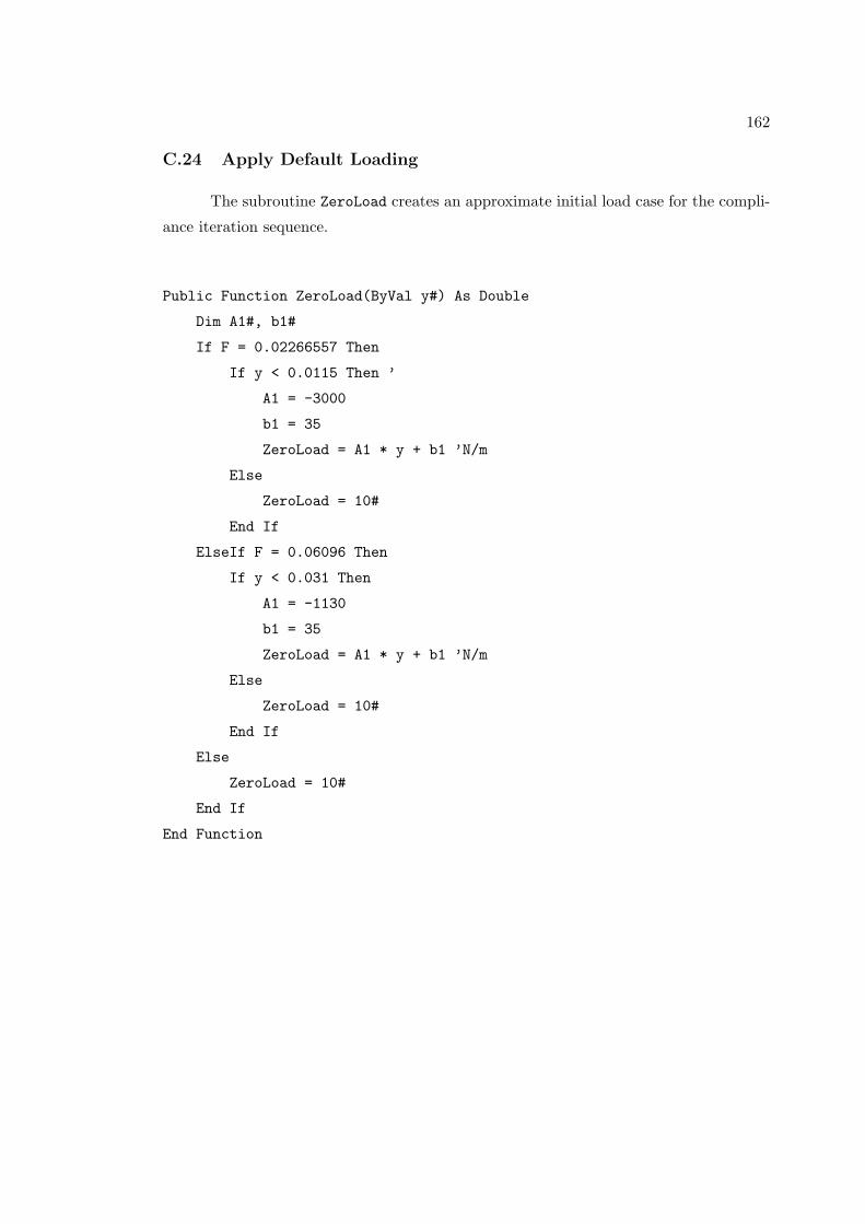
162

C.24 Apply Default Loading

The subroutine ZeroLoad creates an approximate initial load case for the compli-

ance iteration sequence.

Public Function ZeroLoad(ByVal y#) As Double

Dim A1#, b1#

If F = 0.02266557 Then

If y < 0.0115 Then ’

A1 = -3000

b1 = 35

ZeroLoad = A1 * y + b1 ’N/m

Else

ZeroLoad = 10#

End If

ElseIf F = 0.06096 Then

If y < 0.031 Then

A1 = -1130

b1 = 35

ZeroLoad = A1 * y + b1 ’N/m

Else

ZeroLoad = 10#

End If

Else

ZeroLoad = 10#

End If

End Function

163

C.25 Open A Saved Data Set

The subroutine SavedLoad opens a current loading save file for use by the pro-

gram.

Public Function SavedLoad(ByVal yi#, sl%, Yloc#(), LegL#()) As Double

Dim N#, m%, N2#, K%, yil%, yiu%, maxL#

If even(sl) Then

sl = sl - 1

End If

yil = UBound(Yloc)

K = UBound(LegL)

If CInt(yi) = yi And yi > 0 Then

N = Yloc(yi)

m = CInt((1 + yi - sl) / 2 - 0.1)

Else

N = yi

m = 1 - nem

yiu = 3

Do While N > Yloc(yiu) And yiu < yil

m = m + 1

yiu = m * 2 + sl

Loop

yi = m * 2 + sl - 1

End If

Dim rflag%

If m <= 0 Then m = 1: rflag = 1

If m > K / 3 Then m = K / 3: rflag = 1

yiu = m * 2 + sl

yil = yiu - 2

N = Yloc(yiu) - N ’distance from yi to end of element

N2 = Yloc(yiu) - Yloc(yil) ’total length of element

164

N = -N / N2 * 2 + 1 ’eta on the -1 to 1 range

SavedLoad = LegL(m * 3 - 2) + LegL(m * 3 - 1) * r3 * N + _

LegL(m * 3) * r5 / 2 * (3 * N ^ 2 - 1)

End Function

C.26 Rotate the Node Plane

The subroutine NodesRot takes an axial position of nodes and rotates the set to

introduce a helix to the model.

Public Sub NodesRot(Nodes() As Double, ang#)

Dim X#, y#, J%, ju%

ju = UBound(Nodes, 2) ’ nodes)

For J = 1 To ju

X = Nodes(1, J)

y = Nodes(2, J)

Nodes(1, J) = X * Cos(ang) - y * Sin(ang)

Nodes(2, J) = X * Sin(ang) + y * Cos(ang)

Next J

End Sub

165

References

[1] J. E. Shigley and J. Uicker, Theory of Machines and Mechanisms, McGraw-Hill

Inc., 1980.

[2] W. A. Tuplin, Involute Gear Geometry, Chatto and Windus, 1962.

[3] S. L. Harris, Proceedings of the Institute of Mechanical Engineers 172, 87 (1958).

[4] R. W. Gregory, S. L. Harris, and R. G. Munro, Proceedings of the Institute of

Mechanical Engineers (1963).

[5] W. D. Mark, Journal of the Acoustical Society of America 63, 1409 (1978).

[6] W. D. Mark, Journal of the Acoustical Society of America 66, 1758 (1979).

[7] T. G. Chondros, The development of machine design as a science from classical

times to modern era, in International Symposium on History of Machines and

Mechanisms: Proceedings of HMM 2008, edited by H.-S. Yan and M. Ceccarelli,

pages 59–68, New York, NY, 2009, Springer.

[8] T. Koetsier, Mechanism and machine science: Its history and its identity, in Inter-

national Symposium on History of Machines and Mechanisms - Proceedings HMM

2000, edited by M. Ceccarelli, pages 5–26, Norwell, MA, 2000, Kluwer Academic

Publishers.

[9] A. D. Dimarogonas, The Machine: A Historical Introduction, chapter 0, pages 1–33,

John Wiley and Sons, Inc., New York, NY, 2001.

[10] L. P. Euler, Supplementum de figura dentium rotarium, 1765.

[11] J. D. Smith, Gear Noise and Vibration, Marcel Dekker, Inc., New York, NY, second

edition, 2003.

[12] H. Walker, The Engineer 166, 409 (1938).

[13] D. B. Welbourn, Fundamental knowledge of gear noise - a survey, in Noise and

Vibrations of Engines and Transmissions, pages 9–14, London, 1979, Cranfield.

[14] D. R. Houser, Gear Noise Sources and Their Prediction Using Mathematical Models,

chapter 16, pages 213–222, Society of Automotive Engineers, 1990.

166

[15] W. D. Mark, Elements of Gear Noise Prediction, chapter 21, pages 735–769, John

Wiley and Sons, Inc., 1992.

[16] R. G. Munro, A review of the theory and measurement of gear transmission er-

ror, in Proceedings of the Institution of Mechanical Engineers: First International

Concerence: Gearbox Noise and Vibration, pages 3–10, Institution of Mechanical

Engineers, 1990.

[17] H. N. Ozguven and D. R. Houser, Journal of Sound Vibration 125, 71 (1988).

[18] R. G. Munro, N. Yildirim, and D. M. Hall, Optimum profile relief and transmission

error in spur gears, in Proceedings of the Institution of Mechanical Engineers: First

International Concerence: Gearbox Noise and Vibration, pages 35–42, Institution

of Mechanical Engineers, 1990.

[19] R. G. Munro, N. Yildirim, and D. L. Hall, Gearbox noise and vibration , 35 (1990).

[20] A. Kahraman and G. W. Blankenship, Journal of Mechanical Design 121, 313

(1999).

[21] F. L. Litvin et al., Computer methods in applied mechanics and engineering 192,

3619 (2003).

[22] F. L. Litvin, J. Lu, D. P. Townsend, and M. Howkins, Mechanism and machine

theory 34, 123 (1999).

[23] F. L. Litvin, A. Fuentes, A. Demenego, D. Vecchiato, and Q. Fan, New developments

in the design and generation of gear drives, in Proceedings of the Institution of

Mechanical Engineers, Part C: Journal of Mechanical Engineering Science, volume

215, pages 747–757, Professional Engineering Publishing, 2001.

[24] S. Chang, D. R. Houser, and J. Harianto, Tooth flank corrections of wide face

width helical gears that account for shaft deflections, in Proceedings of the 9th

International Power Transmission and Gearing Conference (AGMA Fall Technical

Conference), Chicago, IL, ASME / AGMA.

[25] P. Wagaj and A. Kahraman, Impact of tooth profile modifications on the transmis-

sion error excitation of helical gear pairs, in Proceedings of ESDA2002: 6th Biennial

Conference on Engineering Systems Design and Analysis, 2002.

[26] A. Andersson and L. Vedmar, Journal of Sound and Vibration 260, 195 (2003).

167

[27] D. R. Houser, Research of the Ohio State University gear dynamics and gear noise

research laboratory, in Gearbox noise and vibration: First International Conference,

9-11 April 1990, Churchill College, University of Cambridge, page 19, Published for

the Institution of Mechanical Engineers by Mechanical Engineering Publications

Limited, 1990.

[28] D. R. Houser, J. Harianto, N. Iyer, J. Josephson, and B. Chandrasekaren, A

multi variable approach to determining the ‘best’ gear design, in Proceedings of

DETC’2000 ASME Power transmission and gearing conference, 2000.

[29] S. Sundaresan, K. Ishii, and D. R. Houser, Journal of Mechanical Design 113, 318

(1991).

[30] P. Velex and M. Maatar, Journal of Sound and Vibration 191, 629 (1996).

[31] A. Kahraman and G. W. Blankenship, Journal of Mechanical Design 121, 112

(1999).

[32] N. H. Ozguven and D. R. Houser, Journal of Sound and Vibration 121, 383 (1988).

[33] G. Liu and R. G. Parker, Journal of Mechanical Design 130, 121402 (2008).

[34] R. G. Parker, S. M. Vijayakar, and T. Imajo, Journal of Sound and Vibration 237,

435 (2000).

[35] R. V. Baud and R. E. Peterson, Mechanical Engineering 51, 653 (1929).



[38] A. Y. Attia, ASME Journal of Engineering for Industry 86, 333 (1964).

[39] C. Weber, The deformation of loaded gears and the effect on their load carry-

ing capacity, Technical Report 3, British Department of Scientific and Industrial

Research, 1949.

[40] R. W. Cornell, ASME Journal of Mechanical Design 103, 447 (1981).

[41] R. J. Roark and W. C. Young, Roark’s Formulas of Stress and Strain, McGraw-Hill

Inc., sixth edition, 1989.

[42] T. F. Coney and A. Seirig, Journal of Engineering for Industry , 1115 (1973).

168

[43] D. R. Houser et al., Static and dynamic transmission error measurements and predic-

tion for spur and helical gear sets, in Power Transmission and Gearing Conference,

ASME Design Engineering Division.

[44] M. Stegemiller and D. R. Houser, 3d analysis of the base flexibility of gear teeth,

in Proceedings of the 1989 Power Transmission and Gearing Conference, Chicago,

1989.

[45] D. B. Yakubek and D. R. Houser, 3D deflection analysis of gear teeth using both

FEA and a tapered plate approximation, Technical report, AGMA, 1985, AGMA

paper 85FTM4.

[46] W. B. Rockwood et al., Finite elements applied to the nonlinear calculation of tooth

loads and root stresses in high power density gearing, in AIAA/SAE/ASME/ASEE

23rd Joint Propulsion Conference, 1987, Report No. AAIA-87-1811.

[47] M. Umeyama et al., Effects of gear dimension and tooth surface modifications of

the loaded transmission error of a helical gear pair, in Power Transmission and

Gearing Conference, pages 725–732, ASME Design Engineering Division, 1996.

[48] J. J. Coy and C. Hu-Chih, ASME Journal of Mechanical Design 104, 759 (1982).

[49] W. E. Welker, A method for finite element computation of the contact deformation

of gear teeth, Master’s thesis, The Pennsylvania State University, 1996.

[50] E. M. Jankowich, A method for finite-element computation of the contact defor-

mation of helical gear teeth, Master’s thesis, The Pennsylvania State University,

1997.

[51] M. F. Alulis, A method for finite element computation of compliance influence

functions of helical gear teeth, Master’s thesis, The Pennsylvania State University,

1999.

[52] J. E. Shigley and C. R. Mischke, Mechanical Engineering Design, McGraw-Hill

Inc., fifth edition, 1989.

[53] W. D. Mark, Gear Noise, chapter 36, pages 36.1–36.22, McGraw-Hill Inc., 1991.

[54] M. L. Baxter, Jr., Basic theory of gear-tooth action and generation, in Gear

Handbook: The Design, Manufacture, and Application of Gears, edited by D. W.

Dudley, chapter 1, McGraw-Hill Inc., New York, first edition, 1962.

169

[55] D. W. Kammler, A First Course in Fourier Analysis, Prentice Hall, Inc., 2000.

[56] G. Liu and R. G. Parker, Journal of Sound and Vibration 320, 1039 (2009).

[57] J. D. Smith, Helical gear vibration excitation with misalignment, in Proceedings of

the Institution of Mechanical Engineers, Part C: Journal of Mechanical Engineering

Science, volume 208, pages 71–79, Professional Engineering Publishing, 1994.

[58] J. D. Smith, Proceedings of the Institution of Mechanical Engineers, Part C: Journal

of Mechanical Engineering Science 212, 217 (1998).

[59] F. L. Litvin, Q. Lian, and A. L. Kapelevich, Computer Methods in Applied Me-

chanics and Engineering 188, 363 (2000).

[60] E. W. Weisstein, CRC Concise Encyclopedia of Mathematics, CRC Press, 2003.

Vita

Cameron Paul Reagor was born in Great Falls, Montana, on March 11, 1977. He

graduated from Shelby High School in Shelby, Montana, in May, 1995. He received a

Bachelor of Science degree, with honors, in Mechanical Engineering from the Montana

State University in May, 1999. He enrolled in the Ph.D. program in Acoustics at The

Pennsylvania State University in August, 1999.

He currently owns an acoustics consulting business in Montana.

an optimal gear design method for minimization of transmission error and vibration excitation

Documents