an optimum design of on-bottom stability of offshore...

Int. J. Nav. Archit. Ocean Eng. (2013) 5:598~613 http://dx.doi.org/10.2478/IJNAOE-2013-0156

pISSN: 2092-6782, eISSN: 2092-6790

ⓒSNAK, 2013

Corresponding author: Han Suk Choi, e-mail: [email protected] This is an Open-Access article distributed under the terms of the Creative Commons Attribution Non-Commercial License (http://creativecommons.org/licenses/by-nc/3.0) which permits unrestricted non-commercial use, distribution, and reproduction in any medium, provided the original work is properly cited.

An optimum design of on-bottom stability of offshore pipelines on soft clay

Su Young Yu1, Han Suk Choi1, Seung Keon Lee2, Chang Ho Do3 and Do Kyun Kim1

1Graduate School of Engineering Mastership, Pohang University of Science and Technology, Pohang, Korea 2Department of Naval Architecture and Ocean Engineering, Pusan National University, Busan, Korea

3Hyundai Heavy Industries, Co., Ltd., Ulsan, Korea

ABSTRACT: This paper deals with the dynamic effect of pipeline installation and embedment for the on-bottom stabi-lity design of offshore pipelines on soft clay. On-bottom stability analysis of offshore pipelines on soft clay by DNV-RP-F109 (DNV, 2010) results in very unreasonable pipe embedment and concrete coating thickness. Thus, a new procedure of the on-bottom stability analysis was established considering dynamic effects of pipeline installation and pipe-soil interaction at touchdown point (TDP). This analysis procedure is composed of three steps: global pipeline installation analysis, local analysis at TDP, modified on-bottom stability analysis using DNV-RP-F109. Data obtained from the dynamic pipeline installation analysis were utilized for the finite element analysis (FEA) of the pipeline embedment using the non-linear soil property. From the analysis results of the proposed procedure, an optimum design of on-bottom stability of offshore pipeline on soft clay can be achieved. This procedure and result will be useful to assess the on-bottom stability analysis of offshore pipelines on soft clay. The analysis results were justified by an offshore field ins-pection.

KEY WORDS: On-bottom stability; Offshore pipeline; Dynamic effect; Soft clay; Pipeline embedment.

INTRODUCTION

Interest on offshore energy resources has been increasing globally, especially in Brazil, India, China, and other developing countries. The marine world in 2030 will be almost unrecognizable owing to the rise of emerging countries as mentioned, new consumer classes and resource demand (Fang et al., 2013). As development activities for energy demand move to deepwater, many offshore pipelines to transport oil and gas will be installed. The clay soil on seabed below installed pipelines ranges from very soft to very stiff soil. This paper deals with soft and very soft clay soil and the pipelines will be embeded further into the soft soil. The exact behavior between a pipeline and soil is not known. The heaved soil and resistance forces are hence impor-tant aspects. It is important to properly model pipe-soil interaction effects (Bai and Bai, 2005). Pipe embedment depth by pipe-soil interaction has become critical design parameter to design offshore pipeline such as free span and thermal expansion as well as on-bottom stability. On-bottom stability analysis that a pipeline maintains stability on seabed against hydrodynamic load of wave and current has to be considered with a relevant pipe-soil interaction analysis.

The pipelines are under the combined loads such as bending, axial force, and external pressure during installation due to the

Int. J. Naval Archit. Ocean Eng. (2013) 5:598~613 599

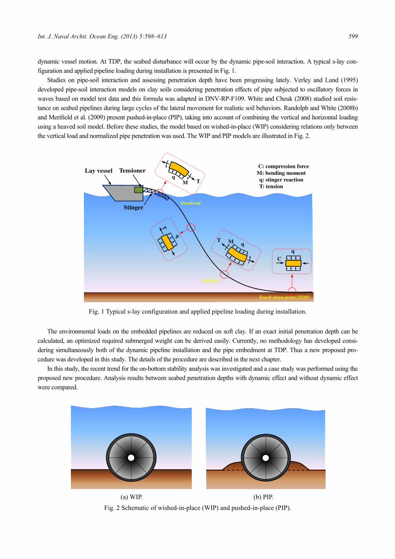
dynamic vessel motion. At TDP, the seabed disturbance will occur by the dynamic pipe-soil interaction. A typical s-lay con-figuration and applied pipeline loading during installation is presented in Fig. 1.

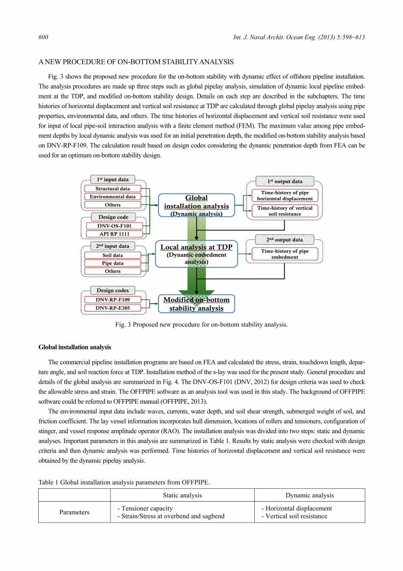
Studies on pipe-soil interaction and assessing penetration depth have been progressing lately. Verley and Lund (1995) developed pipe-soil interaction models on clay soils considering penetration effects of pipe subjected to oscillatory forces in waves based on model test data and this formula was adapted in DNV-RP-F109. White and Cheuk (2008) studied soil resis-tance on seabed pipelines during large cycles of the lateral movement for realistic soil behaviors. Randolph and White (2008b) and Merifield et al. (2009) present pushed-in-place (PIP), taking into account of combining the vertical and horizontal loading using a heaved soil model. Before these studies, the model based on wished-in-place (WIP) considering relations only between the vertical load and normalized pipe penetration was used. The WIP and PIP models are illustrated in Fig. 2.

Fig. 1 Typical s-lay configuration and applied pipeline loading during installation.

The environmental loads on the embedded pipelines are reduced on soft clay. If an exact initial penetration depth can be

calculated, an optimized required submerged weight can be derived easily. Currently, no methodology has developed consi-dering simultaneously both of the dynamic pipeline installation and the pipe embedment at TDP. Thus a new proposed pro-cedure was developed in this study. The details of the procedure are described in the next chapter.

In this study, the recent trend for the on-bottom stability analysis was investigated and a case study was performed using the proposed new procedure. Analysis results between seabed penetration depths with dynamic effect and without dynamic effect were compared.

(a) WIP. (b) PIP.

Fig. 2 Schematic of wished-in-place (WIP) and pushed-in-place (PIP).

C: compression forceM: bending momentq: stinger reactionT: tension

Tq

M

TqM

Cq

Lay vessel

Stinger

Tensioner

Overbend

Sagbend

Touch down point (TDP)

600 Int. J. Naval Archit. Ocean Eng. (2013) 5:598~613

A NEW PROCEDURE OF ON-BOTTOM STABILITY ANALYSIS

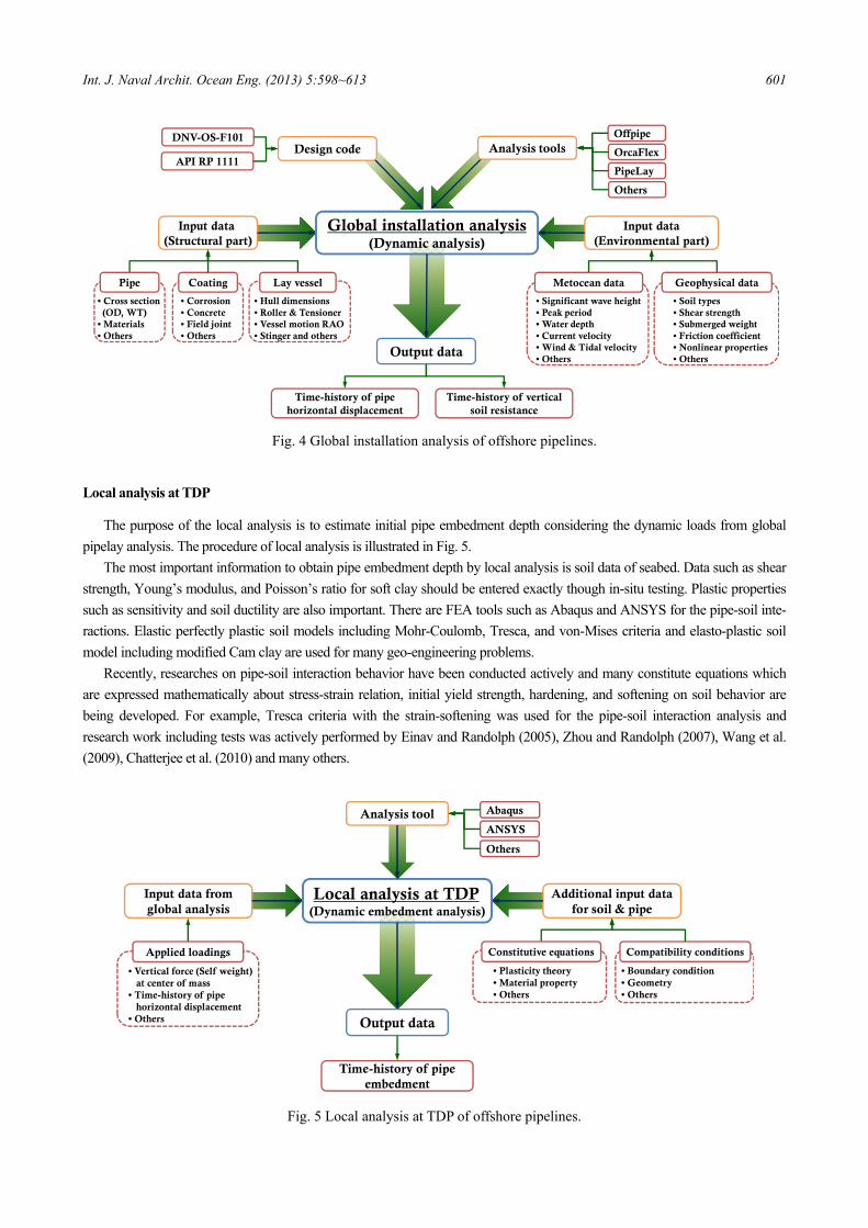
Fig. 3 shows the proposed new procedure for the on-bottom stability with dynamic effect of offshore pipeline installation. The analysis procedures are made up three steps such as global pipelay analysis, simulation of dynamic local pipeline embed-ment at the TDP, and modified on-bottom stability design. Details on each step are described in the subchapters. The time histories of horizontal displacement and vertical soil resistance at TDP are calculated through global pipelay analysis using pipe properties, environmental data, and others. The time histories of horizontal displacement and vertical soil resistance were used for input of local pipe-soil interaction analysis with a finite element method (FEM). The maximum value among pipe embed-ment depths by local dynamic analysis was used for an initial penetration depth, the modified on-bottom stability analysis based on DNV-RP-F109. The calculation result based on design codes considering the dynamic penetration depth from FEA can be used for an optimum on-bottom stability design.

Fig. 3 Proposed new procedure for on-bottom stability analysis.

Global installation analysis

The commercial pipeline installation programs are based on FEA and calculated the stress, strain, touchdown length, depar-ture angle, and soil reaction force at TDP. Installation method of the s-lay was used for the present study. General procedure and details of the global analysis are summarized in Fig. 4. The DNV-OS-F101 (DNV, 2012) for design criteria was used to check the allowable stress and strain. The OFFPIPE software as an analysis tool was used in this study. The background of OFFPIPE software could be referred to OFFPIPE manual (OFFPIPE, 2013).

The environmental input data include waves, currents, water depth, and soil shear strength, submerged weight of soil, and friction coefficient. The lay vessel information incorporates hull dimension, locations of rollers and tensioners, configuration of stinger, and vessel response amplitude operator (RAO). The installation analysis was divided into two steps: static and dynamic analyses. Important parameters in this analysis are summarized in Table 1. Results by static analysis were checked with design criteria and then dynamic analysis was performed. Time histories of horizontal displacement and vertical soil resistance were obtained by the dynamic pipelay analysis.

Table 1 Global installation analysis parameters from OFFPIPE.

Static analysis Dynamic analysis

Parameters - Tensioner capacity - Strain/Stress at overbend and sagbend

- Horizontal displacement - Vertical soil resistance

Structural data


(Dynamic analysis)

Modified on-bottom stability analysis

1st input data 1st output data

Soil data

Time-history of vertical soil resistance

Time-history of pipe horizontal displacement

2nd input data2nd output data

Time-history of pipe embedment

Environmental data

Local analysis at TDP(Dynamic embedment

analysis)

DNV-RP-F109

Design codes

DNV-RP-E305

Others

Others

DNV-OS-F101

Design code

API RP 1111

Pipe data


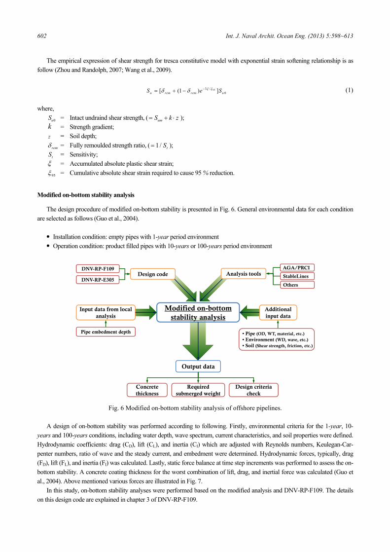
Fig. 4 Global installation analysis of offshore pipelines.

Local analysis at TDP

The purpose of the local analysis is to estimate initial pipe embedment depth considering the dynamic loads from global pipelay analysis. The procedure of local analysis is illustrated in Fig. 5.

The most important information to obtain pipe embedment depth by local analysis is soil data of seabed. Data such as shear strength, Young’s modulus, and Poisson’s ratio for soft clay should be entered exactly though in-situ testing. Plastic properties such as sensitivity and soil ductility are also important. There are FEA tools such as Abaqus and ANSYS for the pipe-soil inte-ractions. Elastic perfectly plastic soil models including Mohr-Coulomb, Tresca, and von-Mises criteria and elasto-plastic soil model including modified Cam clay are used for many geo-engineering problems.

Recently, researches on pipe-soil interaction behavior have been conducted actively and many constitute equations which are expressed mathematically about stress-strain relation, initial yield strength, hardening, and softening on soil behavior are being developed. For example, Tresca criteria with the strain-softening was used for the pipe-soil interaction analysis and research work including tests was actively performed by Einav and Randolph (2005), Zhou and Randolph (2007), Wang et al. (2009), Chatterjee et al. (2010) and many others.

Fig. 5 Local analysis at TDP of offshore pipelines.

Time-history of vertical soil resistance

Time-history of pipe horizontal displacement

Input data(Structural part)

• Cross section(OD, WT)

• Materials• Others

• Corrosion• Concrete• Field joint• Others

• Hull dimensions• Roller & Tensioner• Vessel motion RAO• Stinger and others

Pipe Coating Lay vessel

Offpipe

Input data(Environmental part)

• Significant wave height• Peak period• Water depth• Current velocity• Wind & Tidal velocity• Others

• Soil types• Shear strength• Submerged weight• Friction coefficient• Nonlinear properties• Others

Metocean data Geophysical data

Global installation analysis(Dynamic analysis)

Output data

OrcaFlex

PipeLay

Others

DNV-OS-F101Design code Analysis tools

API RP 1111

Input data from global analysis

Abaqus

Additional input data for soil & pipe

• Plasticity theory• Material property• Others

• Boundary condition• Geometry• Others

Constitutive equations Compatibility conditions

Local analysis at TDP(Dynamic embedment analysis)

Output data

Analysis toolANSYS

Others

• Vertical force (Self weight)at center of mass

• Time-history of pipehorizontal displacement

• Others

Applied loadings

Time-history of pipe embedment


The empirical expression of shear strength for tresca constitutive model with exponential strain softening relationship is as follow (Zhou and Randolph, 2007; Wang et al., 2009).

953 /0[ (1 ) ]u rem rem uS e Sξ ξδ δ −= + − (1)

where,

0uS = Intact undraind shear strength, ( umS k z= + ⋅ ); k = Strength gradient; z = Soil depth;

remδ = Fully remoulded strength ratio, ( 1 / tS= );

tS = Sensitivity; ξ = Accumulated absolute plastic shear strain;

95ξ = Cumulative absolute shear strain required to cause 95 % reduction.


The design procedure of modified on-bottom stability is presented in Fig. 6. General environmental data for each condition are selected as follows (Guo et al., 2004).

• Installation condition: empty pipes with 1-year period environment • Operation condition: product filled pipes with 10-years or 100-years period environment

Fig. 6 Modified on-bottom stability analysis of offshore pipelines.

A design of on-bottom stability was performed according to following. Firstly, environmental criteria for the 1-year, 10-

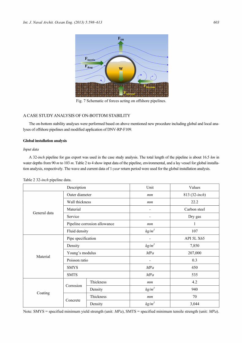
years and 100-years conditions, including water depth, wave spectrum, current characteristics, and soil properties were defined. Hydrodynamic coefficients: drag (CD), lift (CL), and inertia (CI) which are adjusted with Reynolds numbers, Keulegan-Car-penter numbers, ratio of wave and the steady current, and embedment were determined. Hydrodynamic forces, typically, drag (FD), lift (FL), and inertia (FI) was calculated. Lastly, static force balance at time step increments was performed to assess the on-bottom stability. A concrete coating thickness for the worst combination of lift, drag, and inertial force was calculated (Guo et al., 2004). Above mentioned various forces are illustrated in Fig. 7.

In this study, on-bottom stability analyses were performed based on the modified analysis and DNV-RP-F109. The details on this design code are explained in chapter 3 of DNV-RP-F109.

Required submerged weight

Input data from local analysis

Additional input data

• Pipe (OD, WT, material, etc.)• Environment (WD, wave, etc.)• Soil (Shear strength, friction, etc.)


Output data

Pipe embedment depth

Concrete thickness

Design criteria check

AGA/PRCI

StableLines

Others

DNV-RP-F109Design code Analysis tools

DNV-RP-E305


Fig. 7 Schematic of forces acting on offshore pipelines.

A CASE STUDY ANALYSIS OF ON-BOTTOM STABILITY

The on-bottom stability analyses were performed based on above mentioned new procedure including global and local ana-lyses of offshore pipelines and modified application of DNV-RP-F109.


Input data

A 32-inch pipeline for gas export was used in the case study analysis. The total length of the pipeline is about 16.5 km in water depths from 90 m to 103 m. Table 2 to 4 show input data of the pipeline, environmental, and a lay vessel for global installa-tion analysis, respectively. The wave and current data of 1-year return period were used for the global installation analysis.

Table 2 32-inch pipeline data.

Description Unit Values

General data

Outer diameter mm 813 (32-inch)

Wall thickness mm 22.2

Material - Carbon steel

Service - Dry gas

Pipeline corrosion allowance mm 1

Fluid density kg/m3 107

Material

Pipe specification - API 5L X65

Density kg/m3 7,850

Young’s modulus MPa 207,000

Poisson ratio - 0.3

SMYS MPa 450

SMTS MPa 535

Coating

Corrosion Thickness mm 4.2

Density kg/m3 940

Concrete Thickness mm 70

Density kg/m3 3,044

Note: SMYS = specified minimum yield strength (unit: MPa), SMTS = specified minimum tensile strength (unit: MPa).

Flift

Finertia

Fdrag

Ffriction

W

Fnormal


Table 3 Environmental data.


Water depth m 90 to 103

Wave height m 0.75

Wave period s 7

Steady current velocity m/s 0.35

Wave angle to pipe axis deg 90

Current angle to pipe axis deg 90

Table 4 Lay vessel data.


Lpp m 177

B m 35

Depth to 1st deck m 15

Tensiner capability kN 2,000

As mentioned before, dynamic pipelay analyses were performed by using OFFPIPE and its input file requires following

data: pipe, coating, barge, supports including roller and tensioner, stinger geometry, and tension data for static analysis. In addi-tion, time limits for analysis, wave, and laybarge motion RAO data were required for the dynamic analysis.

Calculation method

The formulas for the static pipe stress during pipeline installation in OFFPIPE are as below. The tensile stress (σT) in the pipeline is given by the formula:

2

4= −T

T D whA A

πσ (2)

where, T = External pipe tension ; D = Nominal outside diameter of pipe; w = Specific weight of sea water;h= Depth of the pipe node below sea water surface; A = Cross sectional area of the steel pipe.

The vertical and horizontal bending stresses (σv,h) are calculated, from the vertical and horizontal bending moments, using

the formula:

,, 2

= v hv h

M DI

σ (3)

where, ,v hM = Vertical or horizontal bending moment; I = Cross sectional moment of inertia of the steel pipe.

The hoop stress (σh) in the pipeline is given by:

t2whD

h −=σ (4)

where, t = Steel pipe wall thickness.


The total or equivalent pipe stress ( vmσ ) is calculated from the given tensile, hoop and bending stress using the von-Mises or maximum distortion energy formula:

2 2( ) ( )= + + − +vm c T h c T hσ σ σ σ σ σ σ (5)

where, cσ = Vector sum of the vertical and horizontal bending stresses. For the soil effects, the seabed in OFFFPIPE is modeled as a continuous and elastic frictional seabed model. the vertical soil

reaction as each point is given by:

= ⋅s s sR K δ (6)

where, sK = Vertical stiffness of the soil; sδ = Vertical soil deformation. The FEM is used for static and dynamic analysis in OFFPIPE and the solutions are also fully nonlinear. That is, it is to a

numerical solution of the exact nonlinear differential equation of motion for beam subjected to large deflection and nonlinear material behavior. This FEM represents a nonlinear moment-curvature relationship for a large strain for a pipeline and effects of nonlinear boundary conditions for contacts. The numerical integration to solve equations of motion for the pipeline is used and the dynamic response to environmental forces and the wave by a vessel motion is calculated.

Design criteria in DNV-OS-F101

Check of allowable stress and strain was reviewed by DNV-OS-F101. Table 5 shows the simplified strain criteria of pipe-line’s overbend in the design codes. In sagbend, the design code suggests that the equivalent stress criterion is below 87 % of SMYS and this criterion covers both static and dynamic analyses.

Table 5 Simplified strain criteria of pipeline’s overbend.

Criterion X52 X60 X65 X70

Static analysis (%) 0.205 0.230 0.250 0.270

Dynamic analysis (%) 0.260 0.290 0.305 0.325

Analysis results of the case study

Static analysis results of the case study are summarized in Table 6.

Table 6 OFFPIPE static analysis summaries.

Parameters Unit Values

Tension at top kN 1200

Tension at bottom kN 841.3

Span length from stern m 332

Touchdown length from stern m 312

Pipe gain m 20

Overbend maximum strain % 0.165

Overbend stress ratio to SMYS % 72

Sagbend stress ratio to SMYS % 56

Departure angle at stinger deg 29


Result of required tension at top (safety factor, S.F. = 1.67) is below tensioner capacity. Results at overbend (S.F. = 1.52) and sagbend (S.F. = 1.55) are satisfied with the allowable laying criteria and are shown in Table 7. Fig. 8 shows the total pipe stress percent yield (%) throughout pipelay configuration during installation.

Fig. 8 Pipe elevation profile and yield stress ratio.

Table 7 Results of static analysis of global pipelay.

Calculated lay tension (kN) Overbend (Maximum strain, %) Sagbend (Maximum allowable stress, MPa)

C D S.F. C D S.F. C D S.F.

2,000 1,200 1.67 0.250 0.165 1.52 391.5 (= 450×0.87) 252.7 1.55

Note: C = capacity, D = demand, S.F. = safety factor (C/D). In check of overall static results, support reaction forces and vertical separations between rollers and pipe should be checked

besides above stress/strain limit. After the force equilibrium state of the pipeline is converged by a static analysis, a dynamic laying analysis will be performed. Fig. 9 shows the time history of the lateral displacement at TDP for 500 seconds. The horizontal displacement has about variation of -0.05 to 0.06 m.

Fig. 9 Time history of horizontal displacement of pipe.

Von-Mises pipe stress (%)

Pipe configuration

Wat

er d

epth

(m)

Tot

al v

on-M

ises

pip

e st

ress

(%)

Horizontal coordination (m)

0 50 100 150 200 250 300 350 400 450 500

Time history (s)

-0.08

-0.04

0.00

0.04

0.08

Hor

izon

tal d

ispl

acem

ent (

m)

First 50s are truncated


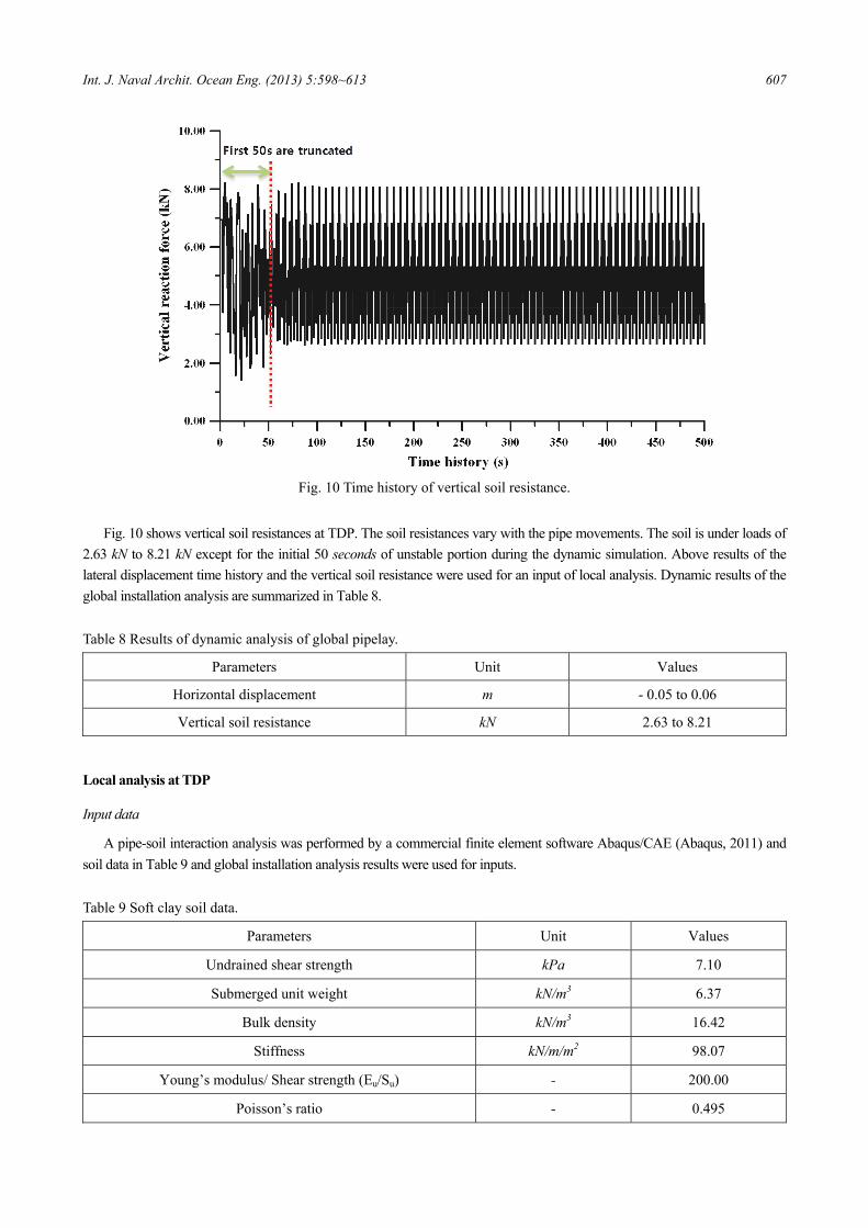
Fig. 10 Time history of vertical soil resistance.

Fig. 10 shows vertical soil resistances at TDP. The soil resistances vary with the pipe movements. The soil is under loads of

2.63 kN to 8.21 kN except for the initial 50 seconds of unstable portion during the dynamic simulation. Above results of the lateral displacement time history and the vertical soil resistance were used for an input of local analysis. Dynamic results of the global installation analysis are summarized in Table 8.

Table 8 Results of dynamic analysis of global pipelay.


Horizontal displacement m - 0.05 to 0.06

Vertical soil resistance kN 2.63 to 8.21

Local analysis at TDP

Input data

A pipe-soil interaction analysis was performed by a commercial finite element software Abaqus/CAE (Abaqus, 2011) and soil data in Table 9 and global installation analysis results were used for inputs.

Table 9 Soft clay soil data.


Undrained shear strength kPa 7.10

Submerged unit weight kN/m3 6.37

Bulk density kN/m3 16.42

Stiffness kN/m/m2 98.07

Young’s modulus/ Shear strength (Eu/Su) - 200.00

Poisson’s ratio - 0.495


Finite Element Model

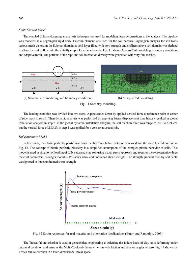
The coupled Eulerian-Lagrangian analysis technique was used for modeling large deformations in the analysis. The pipeline was modeled as a Lagrangian rigid body. Eulerian element was used for the soil because Lagrangian analysis for soil leads serious mesh distortion. In Eulerian domain, a void layer filled with zero strength and stiffness above soil domain was defined to allow the soil to flow into the initially empty Eulerian elements. Fig. 11 shows Abaqus/CAE modeling, boundary condition, and adaptive mesh. The portions of the pipe and soil interaction directly were generated with very fine meshes.

(a) Schematic of modeling and boundary condition. (b) Abaqus/CAE modeling.

Fig. 11 Soft clay modeling. The loading condition was divided into two steps. A pipe settles down by applied vertical force at reference point at center

of pipe mass in step 1. Then dynamic analysis was performed by applying lateral displacement time history resulted in global installation analysis in step 2. In the global dynamic installation analysis, the soil reaction force was range of 2.63 to 8.21 kN, but the vertical force of 2.63 kN in step 1 was applied for a conservative analysis.

Soil constitutive Model

In this study, the elastic perfectly plastic soil model with Tresca failure criterion was used and the model is red dot line in Fig. 12. The concept of elastic perfectly plasticity is a simplified assumption of the complex plastic behavior of soils. This model is used in situation of loading of fully saturated clay soil using a total stress approach and requires the representative three material parameters; Young’s modulus, Poisson’s ratio, and undrained shear strength. The strength gradient term by soil depth was ignored in intact undrained shear strength.

Fig. 12 Strain responses for real material and alternative idealizations (Einav and Randolph, 2005).

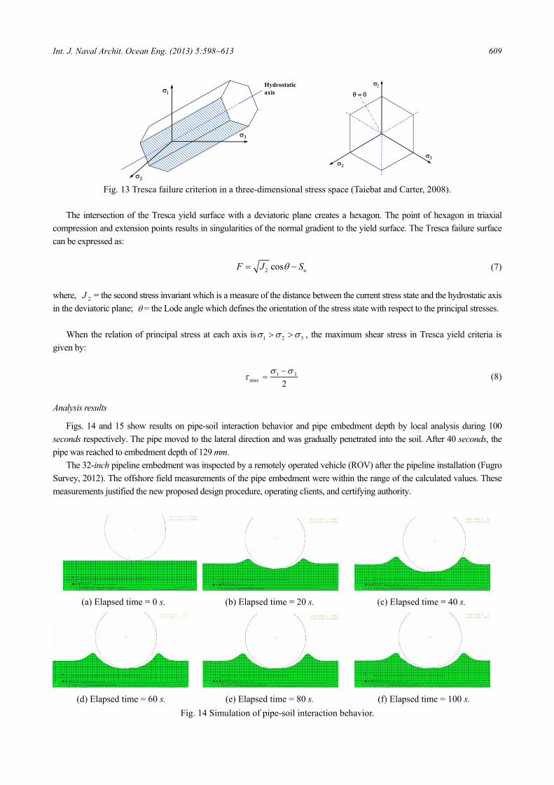
The Tresca failure criterion is used in geotechnical engineering to calculate the failure loads of clay soils deforming under

undraind condition and same as the Mohr-Coulomb failure criterion with friction and dilation angles of zero. Fig. 13 shows the Tresca failure criterion in a three-dimensional stress space.

4Void

Shear strain (γ)

Shea

r st

reng

th (τ

)

Real material response

Ideal perfectly plastic

Ideal inviscid

Elastic perfectly plastic


Fig. 13 Tresca failure criterion in a three-dimensional stress space (Taiebat and Carter, 2008).

The intersection of the Tresca yield surface with a deviatoric plane creates a hexagon. The point of hexagon in triaxial

compression and extension points results in singularities of the normal gradient to the yield surface. The Tresca failure surface can be expressed as:

2 cos uF J Sθ= − (7)

where, 2J = the second stress invariant which is a measure of the distance between the current stress state and the hydrostatic axis in the deviatoric plane; θ = the Lode angle which defines the orientation of the stress state with respect to the principal stresses.

When the relation of principal stress at each axis is 1 2 3σ σ σ> > , the maximum shear stress in Tresca yield criteria is given by:

1 3max 2

σ στ

−= (8)

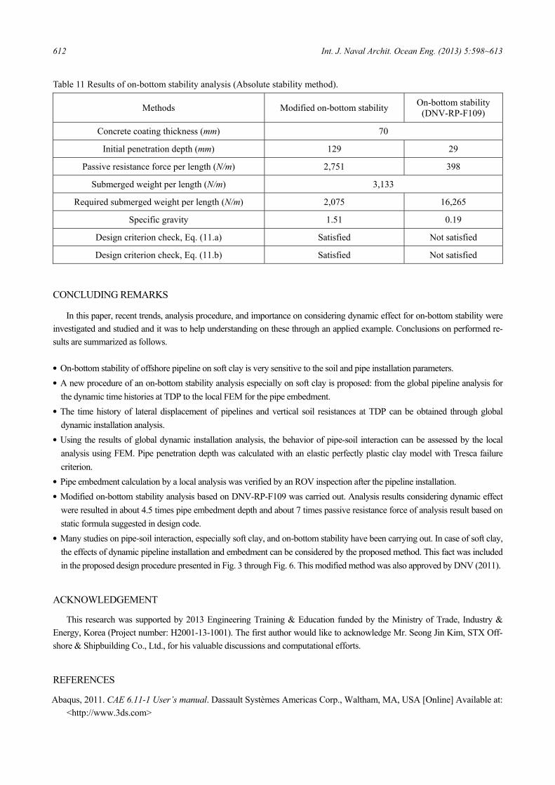
Analysis results

Figs. 14 and 15 show results on pipe-soil interaction behavior and pipe embedment depth by local analysis during 100 seconds respectively. The pipe moved to the lateral direction and was gradually penetrated into the soil. After 40 seconds, the pipe was reached to embedment depth of 129 mm.

The 32-inch pipeline embedment was inspected by a remotely operated vehicle (ROV) after the pipeline installation (Fugro Survey, 2012). The offshore field measurements of the pipe embedment were within the range of the calculated values. These measurements justified the new proposed design procedure, operating clients, and certifying authority.

(a) Elapsed time = 0 s. (b) Elapsed time = 20 s. (c) Elapsed time = 40 s.

(d) Elapsed time = 60 s. (e) Elapsed time = 80 s. (f) Elapsed time = 100 s.

Fig. 14 Simulation of pipe-soil interaction behavior.

σ1

σ2

σ3

Hydrostaticaxis

σ1

σ2

σ3

θ = 0


Fig. 15 Pipeline penetration depth time history by FEM.

Through pipe-soil interaction analysis, penetration depth of 129 mm was calculated. This value represents dynamic effects

and soft clay model. The result, penetration depth of 129 mm, was used to penetration depth for modified on-bottom analysis.


Input data

The water depths in this case study are from 90 to 103 m. For the on-bottom stability analysis, wave data of a 100-year return period at a water depth of 90 m was used for the conservative analysis. Geotechnical data are summarized in Table 9 and environmental data are presented in Table 10.

Table 10 Environmental data.


Water depth range m 90 - 103

Maximum wave height m 13.5

Wave period s 14.2

Steady current velocity m/s 0.58

Wave angle to pipe axis deg 90

Current angle to pipe axis deg 90

Design code criteria

There are two methods in on-bottom stability design suggested by DNV-RP-F109 for the lateral stability. The former is generalized lateral stability method that displacement of pipeline is allowable to 0.5 (Lstable) and 10 times (L10) outside diameter. The latter, called absolute lateral stability method, do not allows displacement of pipe and considers environmental loads associated with a single design oscillation (maximum values).

Generalized stability method does not consider soil effects at seabed. In absolute lateral stability method, many soil effects including load reduction by permeable seabed, penetration, and trenching, passive resistance force, and friction coefficient are considered. Initial penetration depth calculated in local analysis has effects on calculation of load reduction and passive soil resistance force.


DNV-RP-F109, “on-bottom stability design of submarine pipelines”, uses formula for calculation of initial penetration depth from various experiment results by Verley and Lund (1995). This formula considers the penetration resistance without dynamic effects and is indicated in Eq. (9) (Randolph and White 2008a). However, this equation underestimates the penetration depth especially in soft clay and results in very unrealistic submerged pipe weight.

3.2 0.70.3 0.30.0071 0.062

⎛ ⎞ ⎛ ⎞= ⋅ + ⋅⎜ ⎟ ⎜ ⎟

⋅ ⋅⎝ ⎠ ⎝ ⎠

pic c

u u

z V VG GD D S D S

(9)

where,

piz = Initial penetration depth; D = Pipeline diameter; V = Vertical force per unit length; uS = Shear strength;

cG = Soil (clay) strength parameter (= / ( )⋅u sS D γ ); sγ = Dry unit soil weight. After initial penetration depth ( piz ) is calculated, Passive resistance ( RF ) is obtained from following formula.

1.31

0.394.1 ⎛ ⎞⋅ ⋅

= ⋅⎜ ⎟⎜ ⎟⋅ ⎝ ⎠

puR

c c c

zS DFF DG F

(10)

where,

RF = Passive resistance force; cF = Vertical contact force between pipe and soil (= −s zw F );

zF = Vertical hydrodynamic load (lift force). Required submerged weight ( sw ) by obtained concrete thickness should be satisfied with two criteria.

* *1.0

+ ⋅⋅ ≤

⋅ +Y Z

scs R

F Fw F

μγ

μ (11.a)

*1.0⋅ ≤Z

scs

Fw

γ (11.b)

where,

scγ = Safety factor; *YF = Peak horizontal load; *

ZF = Peak vertical load; μ = Coefficient of friction by soil type;

sw = Pipe submerged weight.

Analysis results

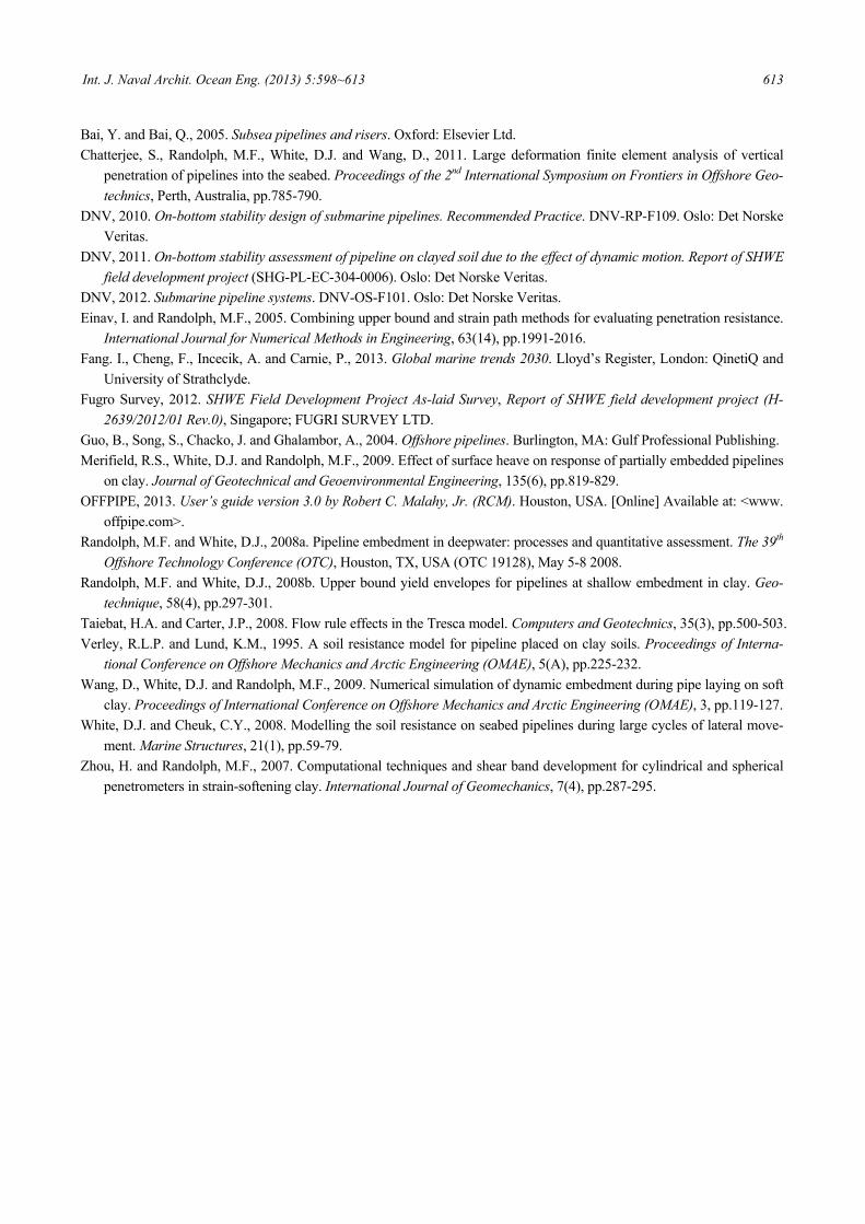
An on-bottom stability analysis was performed by above procedure and the results are summarized in Table 11. The results between initial penetration depths calculated by the present deign code and considering dynamic effects are compared.

Through above results, initial penetration depth which was calculated with effects of pipe-soil interaction on soft clay (FEA) is 129 mm, about 4.5 times that by design code, and this result leads reduced required submerged weight of 2,075 N/m. Calculated concrete thickness of 70 mm in on-bottom stability design with dynamic effects is satisfied with design criteria and specify gravity of this case is enough for stability. But on-bottom stability design considering only static state needs more required submerged weight than previous case since a lot of portion of pipeline is exposed to environmental loads. Concrete thickness corresponding to this required submerged weight is not only thick above 200 mm but also difficult to manufacture. Therefore, this result by second case is not reasonable and importance on consideration of dynamic effect for on-bottom stability is identified.


Table 11 Results of on-bottom stability analysis (Absolute stability method).

Methods Modified on-bottom stability On-bottom stability (DNV-RP-F109)

Concrete coating thickness (mm) 70

Initial penetration depth (mm) 129 29

Passive resistance force per length (N/m) 2,751 398

Submerged weight per length (N/m) 3,133

Required submerged weight per length (N/m) 2,075 16,265

Specific gravity 1.51 0.19

Design criterion check, Eq. (11.a) Satisfied Not satisfied

Design criterion check, Eq. (11.b) Satisfied Not satisfied

CONCLUDING REMARKS

In this paper, recent trends, analysis procedure, and importance on considering dynamic effect for on-bottom stability were investigated and studied and it was to help understanding on these through an applied example. Conclusions on performed re-sults are summarized as follows.

• On-bottom stability of offshore pipeline on soft clay is very sensitive to the soil and pipe installation parameters. • A new procedure of an on-bottom stability analysis especially on soft clay is proposed: from the global pipeline analysis for

the dynamic time histories at TDP to the local FEM for the pipe embedment. • The time history of lateral displacement of pipelines and vertical soil resistances at TDP can be obtained through global

dynamic installation analysis. • Using the results of global dynamic installation analysis, the behavior of pipe-soil interaction can be assessed by the local

analysis using FEM. Pipe penetration depth was calculated with an elastic perfectly plastic clay model with Tresca failure criterion. • Pipe embedment calculation by a local analysis was verified by an ROV inspection after the pipeline installation. • Modified on-bottom stability analysis based on DNV-RP-F109 was carried out. Analysis results considering dynamic effect

were resulted in about 4.5 times pipe embedment depth and about 7 times passive resistance force of analysis result based on static formula suggested in design code. • Many studies on pipe-soil interaction, especially soft clay, and on-bottom stability have been carrying out. In case of soft clay,

the effects of dynamic pipeline installation and embedment can be considered by the proposed method. This fact was included in the proposed design procedure presented in Fig. 3 through Fig. 6. This modified method was also approved by DNV (2011).

ACKNOWLEDGEMENT

This research was supported by 2013 Engineering Training & Education funded by the Ministry of Trade, Industry & Energy, Korea (Project number: H2001-13-1001). The first author would like to acknowledge Mr. Seong Jin Kim, STX Off-shore & Shipbuilding Co., Ltd., for his valuable discussions and computational efforts.

REFERENCES

Abaqus, 2011. CAE 6.11-1 User’s manual. Dassault Systèmes Americas Corp., Waltham, MA, USA [Online] Available at: <http://www.3ds.com>


Bai, Y. and Bai, Q., 2005. Subsea pipelines and risers. Oxford: Elsevier Ltd. Chatterjee, S., Randolph, M.F., White, D.J. and Wang, D., 2011. Large deformation finite element analysis of vertical

penetration of pipelines into the seabed. Proceedings of the 2nd International Symposium on Frontiers in Offshore Geo-technics, Perth, Australia, pp.785-790.

DNV, 2010. On-bottom stability design of submarine pipelines. Recommended Practice. DNV-RP-F109. Oslo: Det Norske Veritas.

DNV, 2011. On-bottom stability assessment of pipeline on clayed soil due to the effect of dynamic motion. Report of SHWE field development project (SHG-PL-EC-304-0006). Oslo: Det Norske Veritas.

DNV, 2012. Submarine pipeline systems. DNV-OS-F101. Oslo: Det Norske Veritas. Einav, I. and Randolph, M.F., 2005. Combining upper bound and strain path methods for evaluating penetration resistance.

International Journal for Numerical Methods in Engineering, 63(14), pp.1991-2016. Fang. I., Cheng, F., Incecik, A. and Carnie, P., 2013. Global marine trends 2030. Lloyd’s Register, London: QinetiQ and

University of Strathclyde. Fugro Survey, 2012. SHWE Field Development Project As-laid Survey, Report of SHWE field development project (H-

2639/2012/01 Rev.0), Singapore; FUGRI SURVEY LTD. Guo, B., Song, S., Chacko, J. and Ghalambor, A., 2004. Offshore pipelines. Burlington, MA: Gulf Professional Publishing. Merifield, R.S., White, D.J. and Randolph, M.F., 2009. Effect of surface heave on response of partially embedded pipelines

on clay. Journal of Geotechnical and Geoenvironmental Engineering, 135(6), pp.819-829. OFFPIPE, 2013. User’s guide version 3.0 by Robert C. Malahy, Jr. (RCM). Houston, USA. [Online] Available at: <www.

offpipe.com>. Randolph, M.F. and White, D.J., 2008a. Pipeline embedment in deepwater: processes and quantitative assessment. The 39th

Offshore Technology Conference (OTC), Houston, TX, USA (OTC 19128), May 5-8 2008. Randolph, M.F. and White, D.J., 2008b. Upper bound yield envelopes for pipelines at shallow embedment in clay. Geo-

technique, 58(4), pp.297-301. Taiebat, H.A. and Carter, J.P., 2008. Flow rule effects in the Tresca model. Computers and Geotechnics, 35(3), pp.500-503. Verley, R.L.P. and Lund, K.M., 1995. A soil resistance model for pipeline placed on clay soils. Proceedings of Interna-

tional Conference on Offshore Mechanics and Arctic Engineering (OMAE), 5(A), pp.225-232. Wang, D., White, D.J. and Randolph, M.F., 2009. Numerical simulation of dynamic embedment during pipe laying on soft

clay. Proceedings of International Conference on Offshore Mechanics and Arctic Engineering (OMAE), 3, pp.119-127. White, D.J. and Cheuk, C.Y., 2008. Modelling the soil resistance on seabed pipelines during large cycles of lateral move-

ment. Marine Structures, 21(1), pp.59-79. Zhou, H. and Randolph, M.F., 2007. Computational techniques and shear band development for cylindrical and spherical

penetrometers in strain-softening clay. International Journal of Geomechanics, 7(4), pp.287-295.

an optimum design of on-bottom stability of offshore...

Documents