AN OVERVIEW OF EXISTING ALGORITHMS FORRESOLVING THE 180◦ AMBIGUITY IN VECTOR

MAGNETIC FIELDS: QUANTITATIVE TESTS WITHSYNTHETIC DATA

THOMAS R. METCALF1, K. D. LEKA1, GRAHAM BARNES1, BRUCE W.LITES2, MANOLIS K. GEORGOULIS3, A. A. PEVTSOV4, G. ALLEN GARY5,JU JING6, K. S. BALASUBRAMANIAM4, JING LI7, Y. LIU8, H. N. WANG9,VALENTYNA ABRAMENKO10, VASYL YURCHYSHYN10, Y.-J. MOON111 Northwest Research Associates, Colorado Research Associates Division, 3380 Mitchell Ln.,Boulder, CO 80301 U.S.A. (metcalf@cora.nwra.com)2 High Altitude Observatory, National Center for Atmospheric Research, P.O. Box 3000, Boulder,CO 80307-3000, U.S.A.3 The Johns Hopkins University Applied Physics Laboratory, 11100 Johns Hopkins Rd., Laurel, MD20723-6099, U.S.A.4 National Solar Observatory, Sunspot, NM 88349, U.S.A.5 NASA/MSFC/NSSTC, Marshall Space Flight Center, Huntsville, AL 35812 U.S.A.6 New Jersey Institute of Technology, Center for Solar-Terrestrial Research, 323 Martin Luther KingBoulevard, Newark, NJ 07102 U.S.A.7 Institute for Astronomy, University of Hawaii, 2680 Woodlawn Dr., Honolulu, HI 96822 U.S.A.8 Stanford University, HEPL Annex, B210, Stanford, CA 94305-4085 U.S.A.9 National Astronomical Observatories, Chinese Academy of Sciences, A20 Datun Rd. ChaoyangDistrict, Beijing 100012 China10 Big Bear Solar Observatory, New Jersey Institute of Technology, 40386 North Shore Lane, BigBear City, CA 92314-9672 U.S.A.11 Korea Astronomy and Space Science Institute, 61-1 Hwaam-dong, Yuseong-gu, Daejeon305-348, South Korea

Received; accepted

Abstract.We report here on the present state-of-the-art in algorithms used for resolving the 180◦ ambi-

guity in solar vector magnetic field measurements. With present observations and techniques, someassumption must be made about the solar magnetic field in order to resolve this ambiguity. Ourfocus is the application of numerous existing algorithms to test data for which the correct answer isknown. In this context, we compare the algorithms quantitatively and seek to understand where eachsucceeds, where it fails, and why. We have considered five basic approaches: comparing the observedfield to a reference field or direction, minimizing the vertical gradient of the magnetic pressure,minimizing the vertical current density, minimizing some approximation to the total current density,and minimizing some approximation to the field’s divergence. Of the automated methods requiringno human intervention, those which minimize the square of the vertical current density in conjunctionwith an approximation for the vanishing divergence of the magnetic field show the most promise.

Keywords:

c© 2006 Springer Science + Business Media. Printed in the USA.

paper.tex; 25/05/2006; 9:44; p.1

2 METCALF ET AL.

1. Introduction

Observations of the vector magnetic field on the surface of the Sun are essential forunderstanding solar magnetic structures in general, and specifically for quantifyingor even predicting solar activity. However, the component of the field perpendic-ular to the line-of-sight, as inferred from observations of linear polarization inmagnetically sensitive spectral lines, has an inherent 180◦ ambiguity in its direc-tion (Harvey, 1969). To fully determine the vector magnetic field, this ambiguitymust be resolved. The reliable resolution of the 180◦ ambiguity is essential forupcoming space- and ground-based vector magnetic field projects such as SOLIS(Jones et al., 2002), Solar-B (Ichimoto and Solar-B Team, 2005; Shimizu, 2004),SDO/HMI (Scherrer and HMI Team, 2005; http://sdo.gsfc.nasa.gov), and ATST(Keil et al., 2003). Looking ahead to these future datasets, a workshop was held atthe National Center for Atmospheric Research in Boulder, Colorado in September2005, to assess the ability of present algorithms to accurately resolve the 180◦

ambiguity.There is no known method for resolving the ambiguity through direct observa-

tion using the Zeeman effect, at least for the single-height observations that are themost popular and well-understood approach for inferring the solar magnetic field.Hence, to resolve the ambiguity, some further assumption on the nature of the solarmagnetic field must be made. Typical assumptions focus on the spatial smoothnessof the field or on minimizing the divergence of the field – the latter, for example,requires approximation when only one height of the field is measured. A numberof different algorithms have been developed to resolve the ambiguity, each makingvarious assumptions on the character of the solar magnetic field. These algorithms,and their assumptions, are detailed in Section 2.

To test their performance, the existing algorithms were applied to model vectormagnetic field data and the results analyzed in a “hare and hounds” exercise. Usingmodel data in this exercise is particularly important because the known correct an-swer can be compared directly to the results from each algorithm. In this paper, webriefly discuss each of the algorithms tested and the data to which the algorithmswere applied. We outline quantitative metrics for judging the performance of thealgorithms when the solution is known, and assess the strengths and weaknesses ofeach algorithm based on its scores for each of the test cases.

2. The Algorithms

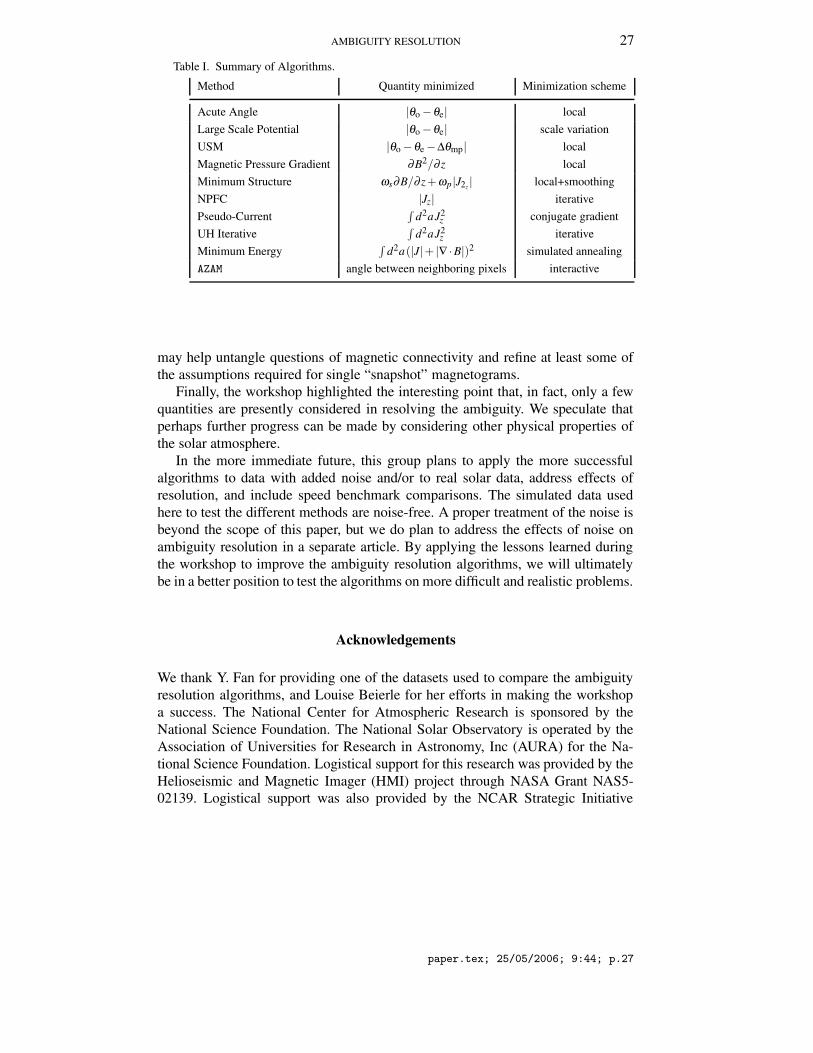
Generally, the algorithms we consider all minimize some physical quantity in orderto arrive at a resolution. In Table I, we summarize both the quantity minimized andthe optimization scheme used for each method. Below, we describe in more detailhow each method is implemented, noting that in some cases there are multiple

paper.tex; 25/05/2006; 9:44; p.2

AMBIGUITY RESOLUTION 3

implementations of the same method. Each algorithm is given a short acronym tofacilitate labeling in the tables and figures.

2.1. ACUTE ANGLE METHOD

Although some areas of the solar atmosphere where vector magnetic field measure-ments are made are clearly not force-free, let alone current-free, it is often usefulto consider a potential, or linear force-free, extrapolation of the magnetic field asa reference for comparison to the observations: Acute Angle Methods resolve the180◦ ambiguity by comparing the observed field to an extrapolated model field. Theazimuth is thus resolved by requiring that some component (i.e., image-plane trans-verse, or heliographic-plane horizontal) of the observed field and the extrapolatedfield make an acute angle, i.e., −90◦ ≤ ∆θ ≤ 90◦, where ∆θ = θo −θe is the anglebetween the observed and extrapolated components. This condition may also beexpressed as Bobs

t ·Bpott > 0, where Bobs

t is the transverse or horizontal componentof the observed field, and Bpot

t is the transverse or horizontal component of theextrapolated field.

The simplest approach is to use the observed, ambiguity-free longitudinal orline-of-sight component of the magnetic field Bl as a boundary condition fromwhich to calculate the potential field. Note that the potential field generated bymatching the line-of-sight field on the boundary will not be the same as the poten-tial field generated using the normal component on the boundary unless the fieldtruly is potential, or the magnetogram is at disk center, so the line-of-sight is thenormal direction. Writing the field as the gradient of a scalar,

B = −∇Φ (1)

guarantees that the field is potential, and substituting this into the vanishing diver-gence of the field

∇ ·B = 0, (2)gives the Laplace equation for the scalar potential:

∇2Φ = 0. (3)

If the vertical component Bz of the magnetic field B is specified inside an area Sthat lays in the plane (x, y), one has the Neumann boundary value problem for theLaplace equation

dΦdz

∣

∣

∣

S= Bobs

z . (4)

One way to solve this problem is to assume that the scalar potential decreasesexponentially with height (Φ ∼ e−κz), and is periodic in the x and y directions. Inthis case, the solution can be expressed in terms of Fourier transforms of the verticalor line-of-sight field on the boundary (Alissandrakis, 1981; Gary, 1989). Clearly,the periodic boundary condition is not valid on the Sun, but the ability to directly

paper.tex; 25/05/2006; 9:44; p.3

4 METCALF ET AL.

use the ambiguity-free line-of-sight component of the field is an advantage of thisformulation. The problem of the periodic boundary condition can be alleviated bypadding the observed line-of-sight field with non-vector data from an instrumentwith a large field-of-view (e.g. SOHO/MDI, Scherrer et al., 1995), padding theboundary data with zeroes, or by assuming the walls of the extrapolation box areperfectly conducting. Each of these approximations are tested below.

Another way to solve this problem is to assume only that B → 0 when r → ∞faster than 1/r, a condition which is reasonable in the case of solar magnetic fields.Then, direct integration of the Green’s function gives the scalar potential as

Φ(x,y,z) =1

2π

∫ Bz(x1,y1)

[(x− x1)2 +(y− y1)2 + z2]1/2 dx1 dy1. (5)

Here the integration is assumed to be done over an infinite plane at z = 0. In thenumerical calculations, the integration is approximated by summing over a gridspecified on the finite area S and this approximation is the main source of compu-tational errors. In applying the Green’s function method to the ambiguity problem,the lower boundary condition, Bobs

z , is approximated by the observed line-of-sightfield Bl , since the vertical field is not known until the ambiguity is resolved. Thisis exact only at disk center, and the error in this assumption grows the further anactive region is from the center of the disk. However, the Green’s function methodis less sensitive to the magnitude of the flux imbalance in a magnetogram thanFFT-based approaches.

While determining the potential field for use in ambiguity resolution seems likea simple and straightforward problem, the many ways in which the extrapolationand the comparison can be implemented lead to significantly different results insome cases. Thus we have considered a range of implementations of the acuteangle method.

In the implementation of J. Jing (NJP), the potential field extrapolation is com-puted using Fourier Transforms with the observed longitudinal field Bl approxi-mating the normal Bz component as the boundary condition, strictly valid only atdisk center. In this implementation, the lower boundary is periodic, not padded withzeroes, and the field of view is forced to be flux-balanced by subtracting a uniformvalue from the lower boundary if the flux-balance condition is not met. The acute-angle comparison is made between the transverse components of the observed fieldand the extrapolated field.

In the implementation of Y. Liu (YLP), the potential field was computed basedon the FFT method proposed by Alissandrakis (1981). This method also assumesthat the observed region is close enough to disk center so that the line-of-sight fieldBl can be treated as the vertical field Bz. The acute angle test is computed for thehorizontal components, that is Bobs

h vs. Bpoth . No additional treatments are applied

to the boundary data, that is, the lower boundary is periodic but any flux imbalanceis represented by a uniform vertical field.

paper.tex; 25/05/2006; 9:44; p.4

AMBIGUITY RESOLUTION 5

In the implementation of K.D. Leka (KLP), the potential field extrapolation iscomputed by Fourier Transform using the unambiguous line-of-sight field as theboundary condition so it does not require the observed region to be close to diskcenter. The area surrounding the observed field is padded with zero longitudinalfield to reduce periodic effects. After an initial ambiguity resolution in the image-plane comparing the observed and computed transverse components (Bobs

t vs. Bpott ),

a new potential field is computed in the heliographic plane using Bz as the boundarycondition and the ambiguity is resolved by comparing the horizontal componentsBobs

h vs. Bpoth .

In the implementation of V. Abramenko and V. Yurchyshyn (BBP), the poten-tial field was computed using a method based on direct integration of the Green’sfunction (Abramenko, 1986),

G(x,y,z) =1

[(x− x1)2 +(y− y1)2 + z2]1/2 , (6)

which is smoothed over each cell of a grid and analytically corrected for the in-fluence of sampling. In applying the Green’s function method to the ambiguityproblem, the lower boundary condition, Bobs

z , is approximated by the observedline-of-sight field Bl , since the vertical field is not known until the ambiguity isresolved. The acute-angle test is then performed between the transverse componentof the observed magnetogram Bobs

t and the horizontal component of the potentialmagnetic field Bpot

h , again under the assumption that the region is not too far fromdisk center.

The implementation of J. Li (JLP) also computes the potential field using aGreen’s function method (Cuperman et al., 1992), with some of the integrals per-formed analytically as described in Cuperman et al. (1990) in order to properlytreat the singularities in the Green’s function. The Green’s function method approx-imates the vertical field with the line-of-sight field as input, but returns heliographiccomponents of the extrapolated field, i.e. the vertical and horizontal field. Theacute angle comparison is then made for transverse component of the observedand extrapolated fields.

The 180◦ ambiguity algorithm used at the Huairou Solar Observatory fromH. N. Wang (HSO) is an acute-angle method which compares the observed field toa linear force-free field (LFFF) computed using a Fourier Transform method withthe observed line-of-sight field Bl as the boundary condition (Wang, 1997; Wanget al., 2001). The force-free parameter α is chosen to maximize S:

S =∫ ∫

P(x,y) dx dy, (7)

where

P(x,y) =|Bobs ·Blff|

BobsBlff (8)

paper.tex; 25/05/2006; 9:44; p.5

6 METCALF ET AL.

and Bobs is the observed transverse field and Blff is the inferred transverse fieldfrom the linear force-free calculation. Low-signal regions are excluded from thisintegral.

The initial value of the force-free factor α is determined according to the lengthscale of the field, and Blff is obtained with a linear force-free model using theobserved line-of-sight field as the boundary condition (there is no padding withzeroes). Then the best fitting linear force-free field for Bobs is found for the valueof α , αbest , which maximizes S in a selected window. The value of αbest is reachedby iteratively changing the value of α . Finally, the azimuth in Bobs is resolved withBlff using the best fitting linear force-free field and the criteria that Bobs ·Blff > 0.The number of windows is determined according to the complexity of Bobs. Onewindow is enough to determine the directions of Bobs in most solar active regions.

2.2. LARGE SCALE POTENTIAL METHOD

It is well established that the magnetic field in the photosphere is not force-free. Amethod to resolve the 180◦ ambiguity, from A. Pevtsov, utilizes two assumptions,that

− magnetograms observed with low spatial resolution can be represented quitewell by force-free and even potential models.

− the deviation from non-potentiality increases with the spatial resolution.

The algorithm (LSPM) begins with a magnetogram smoothed to sufficiently lowspatial resolution so as to be well-represented by the potential field. In successive it-erations, the resolution is gradually increased, which introduces a gradual deviationof the azimuths’ orientation from the potential field. If the resolution is increasedslowly enough, the transition from the potential field to the final (possibly) non-potential field yields a smooth final azimuth that is consistent with the large scalepotential field.

The method starts with a map of the observed longitudinal field, smoothed usinga running boxcar filter. The size of the filter is selected to achieve a significantaveraging (20-30% of the magnetogram’s size). The averaged longitudinal magne-togram is used to calculate the potential field using a Fourier Transform algorithmwith the area surrounding the magnetogram padded with zero longitudinal field.The observed azimuths of the transverse field are then smoothed using the samefilter. The 180◦ ambiguity for the smoothed azimuths is resolved by an acute angletest between the observed and potential transverse field vectors (see Section 2.1,above). The map of the smoothed ambiguity-resolved azimuths is used as a refer-ence for the next step: the size of a boxcar averaging filter is reduced (by about60%), the observed map of azimuths is smoothed using this new averaging filter,and the ambiguity of the smoothed azimuths is again resolved using the acute anglerequirement and the new reference.

paper.tex; 25/05/2006; 9:44; p.6

AMBIGUITY RESOLUTION 7

The cycle of reducing the filter window stops when the size of a filter is equalto the pixel size of the original (observed) magnetogram. Thus, the ambiguity isfirst resolved with a potential field at a very coarse resolution providing a robustresolution for large-scale features. So long as the non-potential structure is re-introduced slowly, the smoothness with the previous step is maintained and thefinal ambiguity resolution should reflect both the large scale potential structure andthe smaller scale non-potential structure of the magnetic field.

2.3. UNIFORM SHEAR METHOD

The Uniform Shear Method (USM; Moon et al., 2003), implemented by Y. Moon,is in some ways similar to the acute angle method. However, instead of choosingthe direction of the observed transverse field to be as close as possible to the corre-sponding potential transverse field, it is instead chosen to be as close as possible tothat direction plus a constant “shear angle offset”, described below. In this manner,the method is more akin to applying the acute angle method to a linear force-freeextrapolation, rather than a potential extrapolation, in that it assumes a consistentsense of twist in the field.

The USM first uses the acute angle method (Section 2.1) to resolve the ambigu-ity with a potential field determined using the Fourier Transform of the longitudinalfield. The magnetic shear angle is then defined as the angular difference betweenthe observed transverse field Bobs

t and the transverse component of the potentialfield Bpot

t . The uniform shear angle offset ∆θmp is initially estimated as the mostprobable value for the magnetic shear angle, assuming that the magnetic shearangle follows an approximately normal distribution. The ambiguity is resolved asecond time by requiring that

−90◦ +∆θmp ≤ θ obs −θ pot ≤ 90◦ +∆θmp, (9)

that is, that the difference between the observed transverse azimuth and the angledefined by the potential azimuth plus a constant angle offset is minimized. A sec-ond estimation of the most probable shear angle is then made by recomputing theshear and fitting a Gaussian to the histogram of the new shear angles, defining ∆θmpas the peak of the Gaussian, and the ambiguity resolution based on Equation (9) isrepeated. The final estimate of ∆θmp is determined to be that which gives the max-imum number of pixels in the range of −80◦ + ∆θmp ≤ θ obs −θ pot ≤ 80◦ + ∆θmpby shifting the second estimation through ±20◦. This estimate, and the resultingambiguity resolution, aims to minimize the number of pixels with a shear anglein either tail of the histogram; it was devised to handle active regions with morecomplex shear angle distributions and minimizes the discontinuities in the numberdistribution of magnetic shear from a statistical point of view.

The final step in the method is effectively a smoothing: the observed transversefield is forced to be in the same direction as the average transverse field of the

paper.tex; 25/05/2006; 9:44; p.7

8 METCALF ET AL.

neighboring pixels. Explicitly,

Bobst ·Bobs

s ≥ 0, (10)

where Bobst is the observed transverse field at a point, and Bobs

s is the mean trans-verse field for the surrounding area.

2.4. MAGNETIC PRESSURE GRADIENT

The magnetic pressure gradient method (MPG), implemented by J. Li, is describedin detail in Cuperman et al. (1993) (see also Harvey, 1969), but the basic under-lying assumptions are that the field at the point of observation is force-free (i.e.,B×(∇×B) = 0) and that the magnetic pressure decreases with height, namely,

∂∂ zB2 < 0. (11)

The force-free field assumption, along with the vanishing divergence of the field,allows the vertical derivative of the magnetic pressure to be written in terms ofhorizontal derivatives

12

∂∂ zB2 = Bx

∂Bz∂x +By

∂Bz∂y −Bz

(

∂Bx∂x +

∂By∂y

)

. (12)

The parameters on the right hand side of the equation are observable magneticcomponents apart from the 180◦ ambiguity in the transverse fields. At disk center,the vertical field and the magnitude of the horizontal components of the field aremeasured, and the two choices for the direction of the horizontal component giveequal magnitude but oppositely signed results for the vertical derivative of the mag-netic pressure. Away from disk center, the observed line-of-sight and transversefields can be transformed into heliographic coordinates for either choice of theambiguity resolution, and Equation (12) still holds. In either case, the ambiguityis resolved, with no iteration, by evaluating ∂B2/∂ z for an initial choice of thedirection of the transverse field. The direction of the transverse field is reversed ateach pixel if ∂B2/∂ z > 0 at that point.

2.5. THE STRUCTURE MINIMIZATION METHOD

The structure minimization method (MS), implemented by M. Georgoulis and in-troduced by Georgoulis et al. (2004), is a semi-analytical method that eliminatesinter-pixel dependencies during the disambiguation. The algorithm proceeds in twosteps: an initial azimuth solution is reached analytically while the final solutionis reached numerically by smoothing the initially disambiguated magnetic fieldvector.

The method starts by considering Ampere’s law for the electric current den-sity. Denoting the magnetic field vector as B = Bb, where B is the magnetic field

paper.tex; 25/05/2006; 9:44; p.8

AMBIGUITY RESOLUTION 9

strength and b is the unit vector along B, the electric current density J is decom-posed into two components, namely J = J1 +J2, where

J1 =cB4π

∇× b and J2 =c

4π(∇B)× b . (13)

The component J1 is due to the curvature of the magnetic field lines, while thecomponent J2 is due to magnetic field gradients and is fully perpendicular to B (seealso the discussion in Zhang, 2001). J2 is the focus for resolving the ambiguity.

For a given vector magnetogram, only the vertical component J2z of J2 canbe readily calculated, though knowledge of the vertical gradient (∂B/∂ z) of themagnetic field strength is sufficient for the complete determination of J2. It isassumed that the magnitude J2 of J2 tends to maximize on the boundaries of mag-netic flux tubes in the solar atmosphere because ∇B maximizes in these surfaceswhere the transition from a magnetized to a non-magnetized medium takes place.Therefore, by minimizing J2, the interfacing current structure between bundles offlux tubes is minimized and hence the assumption of space-filling magnetic fieldsin the active-region atmosphere is enforced.

The magnitude J2 is minimized when

∂B∂ z =

bzb2

x +b2y(bx

∂B∂x +by

∂B∂y ) , (14)

where bx, by, bz are the components of b. Notice that there are only two possiblesolutions for J2 and (∂B/∂ z) (Equations [13] and [14], respectively), for each lo-cation, since the only differentiated quantity is the ambiguity-free magnetic fieldstrength B. To reach the initial azimuth solution, a physical and a geometricalargument is used, namely:

(1) it is assumed that (∂B/∂ z) < 0, namely that the magnetic field strength de-creases with height, in sunspots.

(2) Since J2 ⊥ B, the vector field J2 must be nearly horizontal in plage, becausethe magnetic field B is nearly vertical in these areas. Therefore, it is assumedthat J2z ' 0 in plage.

The above assumptions require that sunspot and plage fields be distinguished, forwhich the continuum intensity is utilized. The continuum intensity, ω p, is normal-ized to fall in the range [0,1], empirically determined for the darkest umbrae andbrightest strong-field regions. To reach the initial azimuth solution in the structureminimization method, we introduce a weighted function

F = (1−ωp)∂B∂ z +ωp|J2z | , (15)

and the azimuth solution is chosen that minimizes the magnitude of F indepen-dently for every location of the magnetogram. This azimuth solution is treated as an

paper.tex; 25/05/2006; 9:44; p.9

10 METCALF ET AL.

initial guess and is smoothed to provide the final solution. The type of smoothingdepends on the location of the active region on the solar disk and consists of a Ja-cobi relaxation process applied to the initial azimuth for active regions fairly closeto disk center, or pattern-recognition filtering of the initial vertical field solution foractive regions far from disk center. The smoothing stops when convergence belowa prescribed fractional tolerance limit is achieved for the strong-field areas of themagnetogram.

2.6. THE NONPOTENTIAL MAGNETIC FIELD CALCULATION METHOD

The Nonpotential Magnetic Field Calculation (NPFC; Georgoulis, 2005) method,implemented by M. Georgoulis, starts by recalling that any closed magnetic struc-ture B rooted in a surface boundary S can be represented by a potential and anonpotential component, Bp and Bc, respectively, i.e.,

B = Bp +Bc . (16)

Notice that (i) all vector fields in Equation (16) are divergence-free and (ii) Band Bp share the same boundary condition for the vertical magnetic field Bz onS, so Bc is horizontal on S. In addition, Bc is responsible for any electric currentspresent since Bp is current-free. From these conditions, and the further assump-tion that ∂Bcz/∂ z vanishes on the boundary S, the nonpotential field Bc becomesanalytically determined on S in terms of the vertical electric current density by

Bc = F−1

[

ikyk2

x + k2yF ( jz)

]

x+F−1

[

−ikxk2

x + k2yF ( jz)

]

y (17)

where F (r) and F−1(r) are the direct and inverse Fourier transforms of r, re-spectively, and jz = 4πJz/c. The condition that ∂Bcz/∂ z vanish on S is equivalentto assuming that ∂Bz/∂ z = ∂Bpz/∂ z on S, i.e. that the vertical derivative of Bz isgiven by the vertical derivative of the vertical potential field.

After calculating Bc, the disambiguation problem requires finding the distri-bution Bz of the vertical magnetic field whose potential extrapolation Bp plus thecalculated nonpotential field Bc (Equation [16]) best matches the observed heli-ographic horizontal magnetic field. This is achieved iteratively, and provides theazimuthal resolution.

Therefore, the problem is to find the vertical current density Jz, or a good proxyof it, prior to the disambiguation. Georgoulis (2005) used an ambiguity-free proxyof Jz derived by extracting from the longitudinal magnetic field Bl any informa-tion on the heliographic horizontal field present in Bl due to projection effects.Specifically, the average of the two possible heliographic ambiguity solutions,Bav = (1/2)(B1 + B2), depends only on Bl , i.e. Bav = ΓBl , where Γ is a knownvector field depending on the direction cosines of the heliographic transformation.Then, a proxy for vertical current density J ′

zp is constructed by applying Ampere’s

paper.tex; 25/05/2006; 9:44; p.10

AMBIGUITY RESOLUTION 11

law to Bav. The calculation of J ′zp is done once, at the beginning of the iterativeprocess for Bz, and the resulting nonpotential field Bc is fixed and used in eachiteration. The magnitude of J ′zp depends on the observing angle to the active re-gion, since the extent of the projection effects on Bl depends on the location of themeasurements. On or close to disk center, J ′

zp ' 0, so the resulting Bc ' 0. In thiscase, the NPFC method degenerates to a simple potential field acute angle method.

2.6.1. Recent ImprovementsThe calculation of the proxy current density in the NPFC method has been im-proved over that described above (Georgoulis, 2005), effectively in response todiscussions at the NCAR workshop, and the results of this new approach are pre-sented here (NPFC2)1. The proxy vertical current density Jzp is now updated ateach iteration i by applying Ampere’s law to the interim resolved magnetic fieldvector, i.e., (4π/c)J(i)

zp = [∇×B(i)]z. Very large values of J(i)zp imply azimuth dis-

continuities, and are set to zero in order not to affect the calculation of Bc. Theseed current density J(0)

zp at the beginning of the iterations uses J ′zp as in Georgoulis

(2005) but also employs the parity-free absolute vertical current density derived bySemel and Skumanich (1998) in the form

J(0)zp = s(J′zp)[sin2 L|J′zp |+ cos2 L|JzSS |] . (18)

In Equation (18), s(J ′zp) is the sign of J ′zp , |JzSS | is the expression of Semel andSkumanich (1998) calculated using the line-of-sight magnetic field components,and L is the heliographic longitude of the location where J (0)

zp is calculated. On orclose to disk center, the major contribution to J (0)

zp comes from |JzSS | which roughlycorresponds to the true magnitude of the vertical current density. Far from diskcenter, J(0)

zp stems mostly from J ′zp which is a lower limit of the true heliographiccurrent.

An additional change is that the field of view in the NPFC method is now paddedwith zeroes to mitigate periodic boundaries in the Fast Fourier Transforms in cal-culating Bp and Bc. When the field of view contains a flux-imbalanced magneticstructure or when strong magnetic flux resides on or close to the boundaries ofthe field of view it is often helpful to place a mirror of the actual image on theextensions which are normally padded with zeroes. This mirroring is done, forexample, with test case #1 described below.

The convergence is tested by means of the number of vector flips or, equiva-lently, the number of flipped Bz-values in each iteration for strong-field locations.The convergence test in the initial NPFC is the one described in Georgoulis (2005)namely a fractional tolerance limit for Bz over the field of view. The number offlips is introduced in the revised NPFC because it is a more readily implementedand easily understood criterion.

1 Code is available at http://sd-www.jhuapl.edu/FlareGenesis/Team/Manolis/codes/ambiguity resolution/

paper.tex; 25/05/2006; 9:44; p.11

12 METCALF ET AL.

2.7. PSEUDO-CURRENT METHOD

The pseudo-current method (PCM; Gary and Demoulin, 1995), implemented byG. A. Gary, resolves the 180◦ ambiguity by minimizing the square of the verti-cal currents of the observed vector magnetogram. The ambiguity is first resolvedusing the potential field acute angle rule (see Section 2.1) to determine an initialvertical electric current density, Jz. The transverse potential field is computed viaan Alissandrakis FFT approach using the line-of-sight corrections, i.e. correct-ing for off-disk center viewing, with boundary buffering equivalent to the FOV.Subsequently, N major local maxima of |Jz| are used to locate the positions Ri =(xi,yi), i = 1, . . . ,N of different “sources” of nonpotentiality.

Each source is used to define an individual Jz patch (Jzi) that is taken as a radiallysymmetric function to allow analytical integration. The current within each patchis defined by

Jzi(r, pi) =Jmax

z j2

[

cos(

πρi|r−Ri|

)

+1]

, |r−Ri| ≤ ρi. (19)

A reference field is generated by using these patches to define vertical line currentsand adding the resultant ad hoc magnetic field to the potential field. The parametersof the reference field are pi = {xi,yi, Jmax

zi ,ρi}, where Jmaxzi is the maximum current

density of the patch and ρi is the characteristic radius. The reference transversefield is used to resolve the ambiguity of the observed field using the acute anglerule. The parameters are then allowed to vary and the functional,

F[J2z ] =

∫ ∫

J2z (x,y, p)dxdy. (20)

is minimized with respect to the set of parameters, {pi}, using a multidimensionalconjugate gradient method.

2.8. U. HAWAI‘I ITERATIVE METHOD

The group at U. Hawai‘i Institute for Astronomy developed an automated iterativemethod (UHIM; Canfield et al., 1993) which (1) performs an initial “acute-angle”resolution based on a potential field calculated via FFT from the observed line-of-sight field, Bl , comparing Bobs

t vs. Bpott (see Section 2.1) (2) uses the resulting ver-

tical field, Bz, to perform a refining “acute-angle” resolution based on a constant-αforce-free field with a specified α , (3) starting from a radial point, e.g. a sunspotumbra, “smooths” by minimizing the angle between each pixel and its neighbors,and, finally, (4) minimizes |Jz| or |∇ · B| according to a specified threshold forthe transverse magnetic field, Bt ; for the latter, ∂Bz/∂ z is determined from theconstant-α force-free field. 2

2 Code is available at http://www.cora.nwra.com/AMBIGUITY WORKSHOP/CODES/mgram.tar

paper.tex; 25/05/2006; 9:44; p.12

AMBIGUITY RESOLUTION 13

The code, written in the IDL language and implemented here by K.D. Leka,includes numerous keywords which govern its operation. Examples of the param-eters that can be set by the operator include the force-free parameter α with whichto compute a force-free field and the minimization threshold alluded to above.Although there are nominal default values, in practice inputs such as α are eitherderived from the data itself or specified by the user, depending on the level ofautonomy required. While the large number of keywords allows for significantflexibility, this approach also provides repeatability. The code is part of a code-treewhich includes a program that computes a best-fit α , selected by minimizing thedifference between the transverse components of the observed field and the linearforce-free field (Leka and Skumanich, 1999; Pevtsov et al., 1995).

Since the method was initially described (Canfield et al., 1993), various im-provements have been made. Most importantly, for the results presented here, theminimization was performed based on J2

z rather than |Jz|; this results in fewer “linecurrents” forming, where conflicting regions of resolution preference “collided”resulting in a line of discontinuity separating two smooth solutions.

Ultimately, it is the minimization of J2z and |∇ ·B| which resolves the ambi-

guity, but, since the space of possible solutions is huge, the prior steps are de-signed to bring the solution close to the correct solution so that the fast, iterativeminimization avoids local minima.

2.9. MINIMUM ENERGY METHODS

The “minimum energy” algorithm (ME1; Metcalf, 1994), implemented by T. Met-calf, simultaneously minimizes both the electric current density, J, and the fielddivergence. Minimizing |∇ ·B| gives a physically meaningful solution and mini-mizing J provides a smoothness constraint. It was shown by Aly (1988) that, for aforce-free field, the magnetic free energy is bounded above by a value proportionalto the maximum value of J2/B2. Since B2 is unambiguous, by minimizing J2 weare minimizing the upper bound on the magnetic free energy. It is in this sense thatthis method is a “minimum energy” algorithm.

The algorithm used here is almost the same as the one described by Metcalf(1994), but one change has been made: the functional to be minimized, E = ∑(|∇ ·B|+ |J|),has been replaced by E = ∑(|∇ ·B|+ |J|)2. Squaring the pseudo-energy functionhas the advantage that more spread out currents are favored over line currents, asdiscussed in the previous section for the UH Iterative method.

The calculation of the vertical electric current density, Jz, is straightforward,requiring only observed quantities in the computation and a choice of the ambigu-ity resolution. However, calculation of ∇ ·B and the horizontal current, Jx and Jy,requires a knowledge of the vertical derivatives of the magnetic field. Variations ofthe magnetic field with height are not normally known (but see Leka and Metcalf,2003), so the vertical derivatives of the field are approximated with a linear force-free field (LFFF) extrapolation using the unambiguous line-of-sight field as the

paper.tex; 25/05/2006; 9:44; p.13

14 METCALF ET AL.

lower boundary condition. The force-free parameter, α , is computed in the samemanner as described above in Section 2.8.

Since the calculation of J and ∇ ·B involves derivatives of the magnetic field,the computation is not local and the number of possible solutions is huge (2N ,where N is the number of pixels; a local algorithm would have only 2N possibil-ities). Further, the solution space has many local minima. Hence, the “simulatedannealing” algorithm (Metropolis et al., 1953; Kirkpatrick et al., 1983) is used tofind the global minimum, an extremely robust approach when faced with a large,discrete problem (there are two and only two possibilities at each pixel) with manylocal minima (Metcalf, 1994).

2.9.1. Recent ImprovementsThe minimum energy approach depends on a linear force-free extrapolation toderive the height dependence of the field. Since the 180◦ ambiguity presents uswith two very different choices at each pixel, the approximate height dependenceof the field computed from the constant α extrapolation is often adequate.

However, it is well known that α is far from constant in typical solar activeregions (Leka, 1999; Pevtsov et al., 1994). Hence a modification to the originalapproach has been implemented, the “non-linear minimum energy method” (ME2),which partially relaxes the constant α assumption. While it would be ideal touse a full non-linear force-free field (NLFFF) extrapolation to derive the verti-cal field structure, this is too slow given today’s computing resources. Hence, weapply the above minimum energy algorithm locally within the magnetogram. Themagnetogram is divided into a number of overlapping tiles; the best value of thelinear force-free α is then computed separately for each tile, in effect allowingα to vary over the field of view. A LFFF extrapolation is computed over thefull field-of-view for each value of α , and the height dependence of the mag-netic field is taken for each tile from the LFFF extrapolation with the value ofα appropriate for that tile. That is, a map of the vertical structure of the field isconstructed from these tiles for which Jx, Jy and ∂Bz/∂ z are computed for the fullmagnetogram. The algorithm then proceeds as above using simulated annealing tominimize E = ∑(|∇ ·B|+ |J|)2.

2.10. THE HAO AZAM UTILITY

As part of the software developed for the HAO/NSO Advanced Stokes Polarimeter(Elmore et al., 1992), the utility “AZAM”, was developed in IDL for the interactiveresolution of the azimuth ambiguity. In addition to ambiguity resolution, it candisplay the vector field results in a variety of ways. AZAM has a common goalwith methods that minimize both the current (by imposing smoothness) and anapproximation to the divergence (by matching expectations of solar structure).

In simple terms, AZAM, implemented here by B. Lites, allows the user to inter-actively “mouse-over”, or “paint”, azimuth choices in either the observer’s or the

paper.tex; 25/05/2006; 9:44; p.14

AMBIGUITY RESOLUTION 15

local solar reference frame. Within a chosen pixel sub-area (ranging from 2× 2to 16× 16 pixels in powers of 2), it sets the selection of ambiguity according toone of a variety of rules. One such rule, used here, chooses the azimuth such thatall points within the sub-area have an azimuth resolution closest to their nearestneighbors. For the 2×2 case, it selects the solution with the maximum sum of thedot products of the transverse field at neighboring pixels in the cardinal directions.For larger sub-areas, it starts by breaking the sub-area down into 2× 2 blocks,maximizes the sum of the neighboring pixel dot products within each block, thenscales up by factors of 2 until reaching the full size of the sub-area.

By “mousing-over” the image, one may set the ambiguity resolution to mini-mize local discontinuities, although this does not necessarily produce the minimummagnitude of the vertical current density within a chosen pixel sub-area. AZAMallows a variety of initial guesses, including the closest resolution to a potential(current free) field solution. Furthermore, it is possible to apply a local smoothingover the whole image to minimize discontinuities. One typically starts the interac-tive resolution from the centers of unipolar sunspot umbrae where the horizontalfield must diverge (converge) away from the center of the umbra for positive (neg-ative) polarity. This sets the ambiguity resolution locally, and one typically worksoutward from the sunspot centers. The solution is deemed to have been reachedwhen the operator is satisfied with the results.

3. Comparisons

To test the performance of the algorithms, we must have data sets for which thecorrect ambiguity resolution is known. Presently, the only ways to obtain such datasets are from MHD simulations, or from analytic solutions to the MHD equations.After applying the algorithms to these data sets, we must have quantitative meansfor assessing their performance. Here we outline the two data sets used, the metricsdevised, and, finally, discuss the results for each of the algorithms.

3.1. THE HARES

For this experiment, two “hares” were used, selected to challenge the algorithmswith various aspects of solar active regions known to be problematic for resolvingthe ambiguity in observational data. However, in both cases, the solution is pro-vided on a grid that is sufficiently fine to resolve all the structure in the magneticfield, but the number of grid points is small enough that no smoothing or interpo-lating is required by any of the methods except the LSPM. Thus no attempt is madeto investigate the sensitivity of the methods to issues of spatial resolution.

3.1.1. Case #1: Twisted Fluxrope in a Potential-Field Arcade, µ = 1.0The first test case is a “photospheric” vector magnetogram constructed from theMHD model of Fan and Gibson (Fan and Gibson (2003); Fan and Gibson (2004)),

paper.tex; 25/05/2006; 9:44; p.15

16 METCALF ET AL.

0 50 100 150 2000

50

100

150

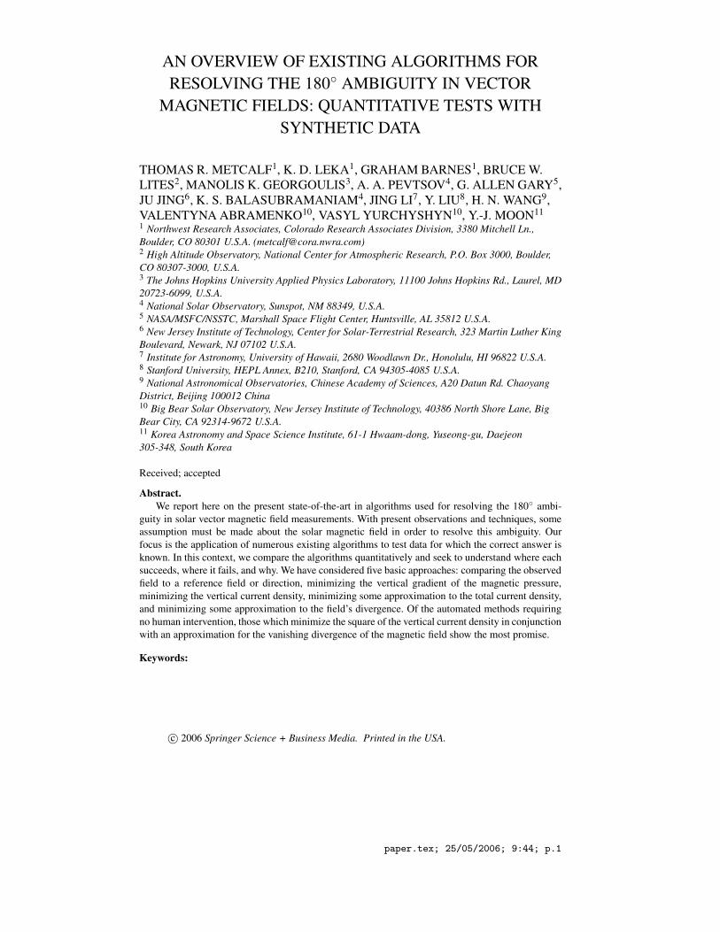
Figure 1. Vector magnetic field at z = 0.006L from the numerical simulation of Fan and Gibson(2004), at their timestep 56. Underlying “continuum image” is a reverse-color image of B2; posi-tive/negative vertical magnetic flux is indicated by red/blue contours at 100, 1000, 2000 G, and themagnetic neutral line is also indicated by the black contour. Horizontal magnetic field is plotted atevery 5th pixel, with magnitude proportional to arrow length. Tickmarks are in units of pixels.

provided courtesy of Y. Fan. The simulation emerged a twisted magnetic flux rope,with approximately constant force-free parameter α into an overlying potential“arcade” field. A “snapshot” at time-step 56 was the source of the boundary field,at z = 0.006L (L is the length scale for the model, effectively the box-length in the ydirection), or slightly above the lower surface (see Figure 1). At this layer the fieldis forced (Fan and Gibson, 2004; Leka et al., 2005) but continuous; relevant factorsfor this project are that it appeared at “disk center” such that Bl = Bz on a grid of240×160 pixels, each 1.0′′2, and the magnetic neutral line included a “bald patch”(Gibson et al., 2004), where the horizontal field traverses the magnetic neutral linefrom negative to positive polarity. Additionally, the presence of both the flux-ropefootpoints and the arcade meant that this magnetogram included both potentialfields and regions that were forced (i.e. J×B 6= 0) and hence far from potential.Finally, the simulation used perfectly conducting side walls, so that no field linescould escape from the edges of the box.

paper.tex; 25/05/2006; 9:44; p.16

AMBIGUITY RESOLUTION 17

0 50 100 150 200 250 3000

50

100

150

200

250

300

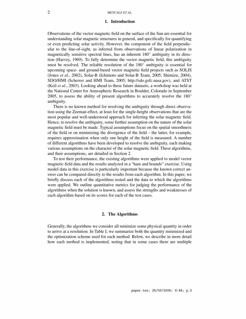
Figure 2. Vector magnetic field for the multi-polar structure in image coordinates. Underlying “con-tinuum image” is a reverse-color image of B2; positive/negative vertical magnetic flux is indicated byred/blue contours at 100, 1000, 2000 G, and the magnetic neutral lines are also indicated by the blackcontour. Horizontal magnetic field is plotted at every 5th pixel. Tickmarks are in units of pixels.

3.1.2. Case #2: Multi-polar constant-α Structure, µ 6= 1.0The second test case is a “chromospheric” vector magnetogram constructed from acollection of point sources located on a plane below the surface. The contributionto the field of each source is calculated using the Green’s function given by Chiuand Hilton (1977) with a constant value of the force-free parameter α . The use of asingle value for α means that the field is everywhere force-free. Four of the sourcesare distributed according to the discussion in Titov et al. (1993) to produce a “baldpatch” along part of the neutral line. A number of additional sources are used toproduce a distribution of flux that has the appearance of an active region (Figure 2).

Although the net charge of all the sources vanishes, one of the sources is placedoutside of the field of view, so the resulting magnetogram is not flux balanced, as istypical for a real vector magnetogram. The field is then calculated on a regular gridof 300×0.5′′2 in the image plane, with the center of the field of view at effectivelyN 18◦, W 45◦, so that the line-of-sight field is distinctly different from the normalcomponent of the field.

paper.tex; 25/05/2006; 9:44; p.17

18 METCALF ET AL.

3.2. THE METRICS

For a quantitative comparison of the methods described above, various metrics,M , were employed which highlighted the successes and failures in different ways.For each, the “solution” provides an azimuth choice θs which is compared to the“answer”’s azimuth choice θa, all in the image (or “instrument” or “observer”)plane resulting in a map of ∆θ that will be either 0◦ or ± 180◦. The metrics werecomputed according to this map and the field (where relevant) obtained from the“answer” data file. The metrics we adopted are:

− Area: a simple fraction of pixels where the submitted solution agreed withthe answer: Marea = #pixels(∆θ = 0)/#pixels. “Good” is closer to 1.00; “ran-dom” would give 0.50.

− Flux: The fraction of the magnetic flux, computed using the answer’s Bz,where ∆θ = 0: Mflux = ∑(|Bz|∆θ=0)/∑(|Bz|). Again, “good” is closer to 1.00;“random” would give 0.50.

− Strong Horizontal Field: The fraction of strong horizontal magnetic fieldwhich was correctly resolved. Both model field test cases were scaled simi-larly with regards to field strengths in the “spots”, etc. and a threshold of 500 Gfor the horizontal was adopted above which Bh was considered strong. Then,calling this strong-horizontal-field Bh(s), this metric is computed as MBh(s) =

∑(Bh(s)∆θ=0)/∑(Bh(s)), and again, “good” is closer to 1.00; “random” wouldgive 0.50.

− Vertical Current: In a different approach, the vertical currents were com-puted for both the submitted solutions and the answer, and compared. In thismetric, the solution is rewarded where it is correct and penalized where it isincorrect:

MJz = 1− ∑(|Jz(answer)− Jz(solution)|)

2∑(|Jz(answer)|). (21)

MJz has been constructed such that “good” is still closer to 1.00, and nor-malized such that a value of 0.00 would occur if the current were exactlyreversed at each pixel; scores less than 0.00 indicate the presence of strongline currents. A score of about 0.00 can also be attained with a combinationof exactly reversed currents and moderate line currents.

3.3. THE RESULTS

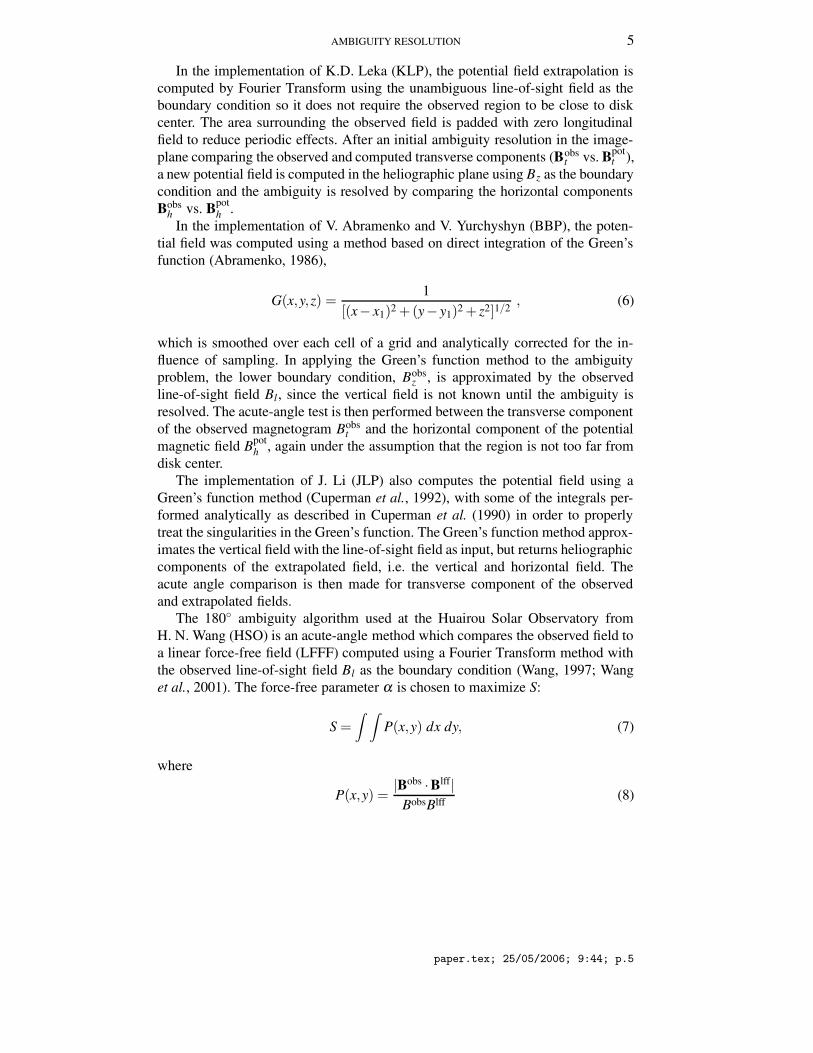
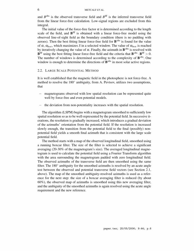
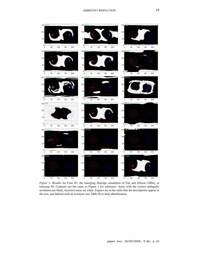
The results are shown in Table II, and Figures 3 and 4. Below, we summarize howeach method performed, highlighting the strengths and the weaknesses of each.

The acute angle methods make a useful benchmark for comparison with othermethods. They are fast, automatic, and simple to implement. To add value, the more

paper.tex; 25/05/2006; 9:44; p.18

AMBIGUITY RESOLUTION 19

0 50 100 150 2000

50

100

150

NJP

0 50 100 150 2000

50

100

150

YLP

0 50 100 150 2000

50

100

150

KLP

0 50 100 150 2000

50

100

150

BBP

0 50 100 150 2000

50

100

150

JLP

0 50 100 150 2000

50

100

150

HSO

0 50 100 150 2000

50

100

150

LSPM

0 50 100 150 2000

50

100

150

USM

0 50 100 150 2000

50

100

150

MPG

0 50 100 150 2000

50

100

150

MS

0 50 100 150 2000

50

100

150

NPFC

0 50 100 150 2000

50

100

150

NPFC2

0 50 100 150 2000

50

100

150

PCM

0 50 100 150 2000

50

100

150

UHIM

0 50 100 150 2000

50

100

150

ME1

0 50 100 150 2000

50

100

150

ME2

0 50 100 150 2000

50

100

150

AZAM

0 50 100 150 2000

50

100

150

TMC

Figure 3. Results for Case #1, the emerging fluxrope simulation of Fan and Gibson (2004), attimestep 56. Contours are the same as Figure 1 for reference. Areas with the correct ambiguityresolution are black, incorrect areas are white. Figures are in the order that the descriptions appear inthe text, and labeled with an acronym (see Table II) to help identification.

paper.tex; 25/05/2006; 9:44; p.19

20 METCALF ET AL.

0 50 100 150 200 2500

50

100

150

200

250

NJP

0 50 100 150 200 2500

50

100

150

200

250

YLP

0 50 100 150 200 2500

50

100

150

200

250

KLP

0 50 100 150 200 2500

50

100

150

200

250

BBP

0 50 100 150 200 2500

50

100

150

200

250

JLP

0 50 100 150 200 2500

50

100

150

200

250

HSO

0 50 100 150 200 2500

50

100

150

200

250

LSPM

0 50 100 150 200 2500

50

100

150

200

250

USM

0 50 100 150 200 2500

50

100

150

200

250

MPG

0 50 100 150 200 2500

50

100

150

200

250

MS

0 50 100 150 200 2500

50

100

150

200

250

NPFC

0 50 100 150 200 2500

50

100

150

200

250

NPFC2

0 50 100 150 200 2500

50

100

150

200

250

PCM

0 50 100 150 200 2500

50

100

150

200

250

UHIM

0 50 100 150 200 2500

50

100

150

200

250

ME1

0 50 100 150 200 2500

50

100

150

200

250

ME2

0 50 100 150 200 2500

50

100

150

200

250

AZAM

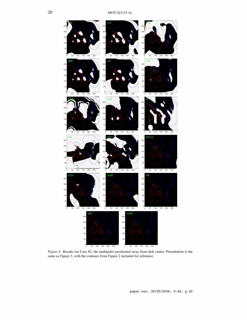
Figure 4. Results for Case #2, the multipoles positioned away from disk center. Presentation is thesame as Figure 3, with the contours from Figure 2 included for reference.

paper.tex; 25/05/2006; 9:44; p.20

AMBIGUITY RESOLUTION 21

complex algorithms need to perform better than the acute angle techniques. If theydo not, there is nothing gained by implementing the more complex algorithms.

None of the acute angle methods scores particularly well on either of the testcases. For the potential field methods, the scores on all the metrics fall in therange 0.6 . M . 0.9 except for the current metric, which is significantly worseat −0.1 . MJz . 0.25. Perhaps the most interesting feature was the wide variationin the scores of the various implementations. Qualitatively, the methods all haddifficulties in the same areas for the flux rope simulation: the arcade field and aband centered between the footpoints of the flux rope. For the arcade field, it is notsurprising that the methods all had difficulties: the side walls of the simulationwere perfectly conducting, so field lines were prevented from leaving the box,whereas the various implementations of the potential field method had periodicboundary conditions (Fourier Transform methods) or open boundary conditions(Green’s function methods), so field lines from the arcade could leave the sides ofthe box. Given knowledge of the side wall boundary conditions, the potential fieldextrapolation could be improved for the arcade.

We have tested this through a modification of the potential field acute anglealgorithm (labeled TMC in Figure 3 and Table II). By reflecting the lower boundaryabout the side walls before applying the Fourier Transform method in the compu-tation of the potential field, the perfectly conducting walls of the arcade field aresimulated. The resulting potential field is used to resolve the ambiguity using theacute angle algorithm. The result is much improved at the top and bottom edgessince the boundary conditions now match those applied in the computation of thearcade field, i.e. no field lines are allowed to leave the box through the side walls.The scores are now M > 0.83 for the first three metrics, and MJz = 0.39. Thisexercise demonstrates the sensitivity of the acute angle algorithms to the particularimplementation of the boundary conditions. Of course, if one knows the true sidewall boundary conditions, it would be helpful to many of the methods, but, in realsolar cases, one does not have this information.

The other area in which the potential field methods had difficulty is part of thearea of highly-nonpotential field in the flux rope. The “bad” part does not follow theneutral line between the foot points of the flux rope, but it does encompass the baldpatch section. This is not surprising, because this is the section in which the hori-zontal field is directed from negative polarity to positive polarity, i.e., “backwards”.While such an orientation is possible with a potential field, it requires special cir-cumstances (Titov et al., 1993). What is perhaps surprising is that the centers of thefoot points of the flux rope are mainly reproduced correctly, so the majority of theflux in the flux rope is correct. The exact area in which the acute angle method wassuccessful depended on the implementation of the potential field extrapolation.This indicates the sensitivity of the acute angle method: a small change in thepotential field can result in a different choice of azimuth over a significant area.It was interesting to note, however, that potential field methods were correct forsome regions in which currents were present, and failed in some regions in which

paper.tex; 25/05/2006; 9:44; p.21

22 METCALF ET AL.

the field truly was potential. Using a linear force-free extrapolation instead of apotential field resulted in scores in the same range except on the current metric,which improved significantly to 0.6 . MJz . 0.7.

The Large Scale Potential Method has difficulties in the same general areas asthe acute angle methods, with one distinct difference: it does not obtain a smoothsolution. There are narrow bands in which the solution flips from correct to in-correct. In some cases, this may improve the area in which the solution is correctslightly, but it comes with a large cost: strong line currents are introduced wherethe solution flips. This results in the much worse scores of MJz = −0.84 (Case #1)and MJz =−0.38 (Case #2), in comparison to the acute angle methods. On the plusside, this algorithm is computationally fast and might be appropriate for automatedprocessing of “quick-look” data.

The Uniform Shear Method performed very similarly to the linear force-freefield acute angle algorithm, both in the scores, with M & 0.65 for all the metricsexcept 0.4 . MJz . 0.5, and in the areas in which it failed. This is not surprisingsince the algorithm assumes a constant shear offset over the full magnetogram; thisdoes not necessarily result in a constant force-free parameter, but it does indicatea similar consistent twisting of the field. Unless the field of view contains only asingle flux tube, it is likely that the distribution of shear angles will not resemblea Gaussian, and indeed may not be unimodal, hence the uniform shear methodis best applied locally, for example along a single sheared neutral line, where themagnitude and sign of the shear is more consistent. This is confirmed by the successof the method along the bald patch in Case #1, and by the high scores on thehorizontal field metric (MBh(s) & 0.9) in both cases.

The Magnetic Pressure Gradient algorithm assumes that the magnetic pressureis decreasing with height. While this is correct over much of the test cases, itis incorrect in some important areas. For example, the magnetic field over baldpatches increases with height (Titov et al., 1993), and the method did indeed failin the vicinity of the bald patches in both test cases. That this algorithm is basedon an (occasionally) incorrect assumption may explain why the algorithm did notscore noticeably better than the potential field acute angle algorithms.

The minimum structure algorithm performed poorly on both test cases, and wasworse than a random selection in Case #1, with M < 0.3 for all metrics. Althoughthe method is computationally fast, the disambiguation relies on the validity of theminimum structure approximation (Equation [14]) as well as additional assump-tions that may break down locally. For example, the assumption (∂B/∂ z) < 0 insunspots is not always correct (Leka and Metcalf, 2003), and the method refersspecifically to sunspot and plage fields, thus misrepresenting other structures suchas canopies or emerging flux regions. We hypothesize that for Case #1 which sim-ulated an emerging flux region, the assumptions were simply not applicable. ForCase #2, the continuum intensity was modeled as proportional to 1−B2/(2B2

max),so the method may have been misled in identifying spots and plage. In addition,

paper.tex; 25/05/2006; 9:44; p.22

AMBIGUITY RESOLUTION 23

the final smoothing is a numerical necessity dictated by the imperfections of theseassumptions and lacks a solid physical background.

It is interesting to compare the Magnetic Pressure method to the MinimumStructure method, as both take the same approach in regions of strong field (sunspots).However, even in strong field regions, there are large areas where the two obtaindifferent results, indicating the large role that the smoothing plays in the MinimumStructure method.

The NPFC algorithm is represented both by results from the original algorithm(Georgoulis, 2005), and the modified version described above. The original algo-rithm did not score better than the acute angle algorithms, however, the modifiedversion scored significantly better, with M & 0.8 for Case #1 and M & 0.98 forCase #2. The improvement can likely be attributed to the more robust estimation ofJz and its iterative updates. In Case #1, which was exactly at disk center, the originalversion of the NPFC algorithm reduced to a potential field ambiguity resolutionbecause J ′zp = 0 from symmetry. The NPFC algorithms are reasonably fast andfully automated.

The Pseudo-Current algorithm performed reasonably well in each test, typicallywith M ≈ 0.8. However, MJz ≈ 0.5, which was similar to the LFFF acute anglemethod and significantly higher than the typical values around 0.0 for the poten-tial field acute angle methods. This algorithm is suited for highly nonpotentialmagnetic field regions, cases where the potential field algorithm fails, as againdistinguished by the MJz metric. The algorithm is local in nature, hence it is fast,automated, and independent of the field of view of the magnetogram. Its goal issimilar to that of the minimum energy solutions, with an optimization schemethat is fast but, in general, unable to guarantee a global minimum. In addition, themethod had difficulty with the arcade field in Case #1, likely for the same reasonsthat the potential field methods failed here: the perfectly conducting walls.

The UH Iterative algorithm scored significantly better for all cases than the var-ious acute-angle methods, with M & 0.88 for all metrics in Case #1 and M & 0.97in Case #2; it scored significantly better for both cases than the other algorithmshighlighted thus-far and was comparable to the revised NPFC. It had fewer dif-ficulties with the arcade field in Case #1, indicating that it is less sensitive tothe potential field extrapolation. This iterative minimization can be classified as“reasonably fast” and fully automated; as such, it may be very appropriate whenthere is a need to balance speed and accuracy.

The two “minimum energy” algorithms scored extremely well for both testcases, on all metrics. The minimum energy and non-linear minimum energy meth-ods had M & 0.99 for each metric on Case #2, while the original implementationhad some minor difficulties with Case #1, resulting in a lowest score of MJz = 0.93.The few pixels that were not treated correctly were at the edge of the field ofview where boundary problems in computing ∇ ·B appear. Both of these minimumenergy approaches are fully automated, but can be classified as slow (minimum

paper.tex; 25/05/2006; 9:44; p.23

24 METCALF ET AL.

energy) and very slow (non-linear minimum energy). As such, they may be bestsuited for magnetograms undergoing detailed analysis.

The AZAM utility was able to successfully recover the correct azimuth for essen-tially every pixel in both test cases, resulting in scores that, for all cases, were 1.0.The test cases have a continuous, smooth variation of the field vector over the sim-ulated field. Because of this, they represent an almost trivial case for AZAM since, ifone is able to select the correct ambiguity resolution at one point in the field, AZAMwill lead to the correct resolution at every other point by working outward from thefirst point. It is therefore not obvious in the case of spatially discontinuous data, forexample as is generally presented by observations, that AZAM will perform betterthan other methods.

A particular advantage of AZAM is that one can manually incorporate other infor-mation that may be helpful for tricky ambiguity resolution problems. Sometimesactive regions require that the choice of azimuth include a discontinuity betweennearest neighbors: that is, there must be a place where the adjacent pixel has anazimuth that is not the selection closest to that of the current pixel. AZAM interac-tively displays the locations of these discontinuities, and allows one to use otherinformation (such as abrupt changes in the intrinsic field strength) to “push” thediscontinuity to locations where it makes some physical sense; i.e. where a largershift in azimuth might be acceptable. The flexibility of AZAM to display differ-ent quantities such as the intrinsic field strength, along side of the azimuth andinclination, are powerful advantages of this method.

Presently, AZAM is not written in a way that is easily adapted to data from othersources, but this update is planned as part of the NCAR Community Spectro-polarimetric Analysis Center (CSAC). Being a manual method, one must becomefamiliar with its usage. Use of AZAM thus remains somewhat of a learned art ratherthan a method based on well-defined physical principles. Furthermore, since itrequires human intervention, it is impractical to use AZAM as a routine method forresolving the ambiguity in upcoming missions, such as Solar-B and SDO. Finally,it is almost impossible for one user to exactly duplicate the ambiguity resolutionof another user for solar data. However, it is likely that AZAM, or some derivative,may remain useful in the future as a procedure to impose final conditioning uponresults from automatic azimuth ambiguity resolution procedures, especially foractive regions that have highly sheared and non-potential features.

4. Summary and Conclusions

Today’s measurements of the solar magnetic field most commonly comprise spec-tropolarimetric data, from which single-height maps of the 180◦ ambiguous vectorare derived. In order to resolve the ambiguity and obtain physically meaningfuldata, some assumption must be made about the solar field. Typically, this assump-tion involves minimizing a quantity which itself depends on the choice of azimuth.

paper.tex; 25/05/2006; 9:44; p.24

AMBIGUITY RESOLUTION 25

Despite the array of methods presented here, the number of quantities chosen tobe minimized is relatively small, and for most of the quantities, it is known thatat least some areas of the Sun are in fact not in a minimum state. We have con-sidered five basic approaches: (i) comparing the observed field to a reference fieldor direction, (ii) minimizing the vertical gradient of the magnetic pressure, (iii)minimizing the vertical current density, (iv) minimizing some approximation to thetotal current density, and (v) minimizing some approximation to the divergence. Inmany algorithms, combinations of these approaches are used.

Many of the variations in the results here are caused not by fundamental differ-ences in the underlying assumptions, but rather by the different implementations.That is, the algorithms implement different methods for calculating the poten-tial field, different optimization or minimization schemes, or varying degrees ofsmoothing performed after an initial resolution is assigned to each pixel. Of theautomated methods, those which minimize some measure of the vertical currentdensity in conjunction with minimizing an approximation for the fields’ divergenceshow the most promise (e.g. ME1, ME2, UHIM, NPFC2), and make assumptionswhich are least obviously violated (an assumption about the vertical derivative ofthe field, linear force-free or potential, is made). For the other methods, it is clearthat the assumptions are violated in some areas: the solar magnetic field is neitherpotential nor linear force-free, so the acute angle methods must fail; the magneticpressure increases with height above bald patches (and likely in sunspot canopies),so the magnetic pressure gradient and the minimum structure methods must fail;except possibly in localized regions, the distribution of magnetic shear need notbe unimodal, let alone Gaussian, so the minimum shear method must fail. Evenwhen there is a quantity that truly is a minimum for the field, the space of possibleambiguity resolutions can contain many local minima, so that a robust optimizationscheme is necessary to reach the true global minimum.

All of the automated methods make use of a potential, linear force free, orsimilar algorithm, at least as a starting condition. In the calculation of these fieldmodels, the treatment of the boundary conditions is important and does affect thefinal outcome. Some methods assume that the observation is close to disk centerand approximate Bz with Blos; the Green’s function algorithms typically make thisassumption. FFT algorithms typically have periodic boundary conditions that canbe ameliorated by padding the boundary with zeros, though padding with zeroesmay not be appropriate if there is strong field at or near the edge of the field-of-view, as in the arcade in Case #1. The presence of nearby unobserved flux impactsthe extrapolations and hence most ambiguity resolution schemes; a large field-of-view is important when resolving the ambiguity. For any automated scheme, it isnow clear that attention to the boundary conditions is very important, as there isunlikely to be a single ideal treatment for all observational cases.

Although it clearly scored the highest in the tests presented here, AZAM requiresmanual input and is not appropriate for automated ambiguity resolution, but it is agood tool for understanding the possibilities for ambiguity resolution in select mag-

paper.tex; 25/05/2006; 9:44; p.25

26 METCALF ET AL.

netograms. For automated processing, the non-linear minimum energy algorithmscored the best, but it is slow. It would be most appropriate for magnetogramswhere the correct answer is paramount and the processing time secondary. Forreasonably fast and reasonably accurate automated ambiguity resolution, the UHiterative method scored best with the revised NPFC2 algorithm a close second.

4.1. WHERE TO GO FROM HERE?

The exercises undertaken in the NCAR workshop highlight the most commonchallenges to ambiguity resolution algorithms, and highlight as well some direc-tions to consider for future research. The errors produced by flux imbalance, andthe influence of magnetic field just outside the field-of-view, can be mitigated byinstruments with larger observing area; the best option of course being routinefull-disk observations which will be provided by SOLIS and by HMI on the SDOmission. Still, such a solution is not immediately available without some seriousthought: for example, all of the algorithms tested here use Cartesian geometry,and full-disk magnetograms will require the use of spherical geometry, except forisolated active regions. Isolated active regions are, however, the exception ratherthan the rule since interconnections between active regions and even across theequator are common.

A common approach among the algorithms is to make assumptions concerningthe vertical structure of the solar magnetic field. Investigations have inferred thedepth- or height-dependence of the magnetic field through sophisticated inversionprocedures for the spectropolarimetric data, e.g. the MISMA (Sanchez Almeida,1997; Sanchez Almeida and Lites, 2000), and SIR (Ruiz Cobo, 1998; Westen-dorp Plaza et al., 2001) approaches. In general, such inversion algorithms requirevery high precision spectropolarimetry and large computational efforts, and theirapplicability to the ambiguity resolution problem has not yet been investigated.More tenable in the short-term is the approach of simultaneous multi-height ob-servations, through either multi-line spectropolarimetry covering heights from thedeep photosphere to low corona, or the use of broad lines such that inversionscan be performed at multiple heights (Metcalf et al., 1995). Again, whether or notthese more sophisticated observations can be routinely applied to the ambiguity-resolution problem is still in the research stage. Additionally, very few instrumentshave the capability of acquiring such data, and even fewer still will be doing soroutinely over the next solar cycle.

What will become routine are temporally well-sampled observations from space-based missions. Although the expected data will have shortcomings to be sure,it will be possible to impose smoothness requirements in the temporal domainin addition to the spatial domain. In this way (albeit with post-facto knowledgeof an active region’s evolution), the characteristics of different quickly-evolvingstructures such as emerging flux regions and moving magnetic features, can betreated appropriately. The information gained on a feature’s temporal evolution

paper.tex; 25/05/2006; 9:44; p.26

AMBIGUITY RESOLUTION 27

Table I. Summary of Algorithms.Method Quantity minimized Minimization scheme

Acute Angle |θo −θe| localLarge Scale Potential |θo −θe| scale variationUSM |θo −θe −∆θmp| localMagnetic Pressure Gradient ∂B2/∂ z localMinimum Structure ωs∂B/∂ z+ωp|J2z | local+smoothingNPFC |Jz| iterativePseudo-Current

∫

d2aJ2z conjugate gradient

UH Iterative∫

d2aJ2z iterative

Minimum Energy∫

d2a(|J|+ |∇ ·B|)2 simulated annealingAZAM angle between neighboring pixels interactive

may help untangle questions of magnetic connectivity and refine at least some ofthe assumptions required for single “snapshot” magnetograms.

Finally, the workshop highlighted the interesting point that, in fact, only a fewquantities are presently considered in resolving the ambiguity. We speculate thatperhaps further progress can be made by considering other physical properties ofthe solar atmosphere.

In the more immediate future, this group plans to apply the more successfulalgorithms to data with added noise and/or to real solar data, address effects ofresolution, and include speed benchmark comparisons. The simulated data usedhere to test the different methods are noise-free. A proper treatment of the noise isbeyond the scope of this paper, but we do plan to address the effects of noise onambiguity resolution in a separate article. By applying the lessons learned duringthe workshop to improve the ambiguity resolution algorithms, we will ultimatelybe in a better position to test the algorithms on more difficult and realistic problems.

Acknowledgements

We thank Y. Fan for providing one of the datasets used to compare the ambiguityresolution algorithms, and Louise Beierle for her efforts in making the workshopa success. The National Center for Atmospheric Research is sponsored by theNational Science Foundation. The National Solar Observatory is operated by theAssociation of Universities for Research in Astronomy, Inc (AURA) for the Na-tional Science Foundation. Logistical support for this research was provided by theHelioseismic and Magnetic Imager (HMI) project through NASA Grant NAS5-02139. Logistical support was also provided by the NCAR Strategic Initiative

paper.tex; 25/05/2006; 9:44; p.27

28 METCALF ET AL.

Table II. Results for Ambiguity Resolution Algorithms.

Solution Fluxtube and arcade Multi-pole at µ 6= 1.0

Marea Mflux MBh(s) MJz Marea Mflux MBh(s) MJz

Acute Angle (potential, FFT)NJP (J. Jing) 0.67 0.49 0.92 -0.07 0.76 0.85 0.87 0.10YLP (Y. Liu) 0.64 0.54 0.90 -0.08 0.82 0.86 0.88 0.08KLP (K.D Leka) 0.75 0.69 0.94 0.25 0.64 0.90 0.73 0.20

Acute Angle (potential, Greens Func.)BBP (V. Yurchyshyn) 0.72 0.65 0.92 0.04 0.78 0.88 0.90 0.25JLP (J. Li) 0.70 0.64 0.90 -0.01 0.71 0.81 0.83 0.13

Acute Angle (LFFF)HSO (H.N. Wang) 0.87 0.70 0.99 0.68 0.85 0.94 0.94 0.60

Large Scale PotentialLSPM (A. Pevtsov) 0.69 0.53 0.89 -0.84 0.69 0.89 0.74 -0.38

Uniform Shear MethodUSM (Y.-J. Moon) 0.83 0.66 1.00 0.50 0.82 0.90 0.89 0.41

Magnetic Pressure GradientMPG (J. Li) 0.74 0.92 0.85 -0.77 0.67 0.79 0.76 -0.41

Minimum StructureMS (M. Georgoulis) 0.22 0.14 0.23 0.18 0.36 0.67 0.58 -0.29

Nonpotential Magnetic Field CalculationNPFC (M. Georgoulis, original) 0.70 0.62 0.92 0.02 0.70 0.90 0.83 -0.00NPFC2 (M. Georgoulis, revised) 0.90 0.77 1.00 0.81 0.99 1.00 1.00 0.98

Pseudo-CurrentPCM (A. Gary) 0.78 0.49 0.98 0.54 0.77 0.82 0.82 0.40

UH IterativeUHIM (K. Leka) 0.97 0.91 1.00 0.88 0.97 0.99 1.00 0.97

Minimum EnergyME1 (T. Metcalf, original) 0.98 0.96 1.00 0.93 1.00 1.00 1.00 0.99ME2 (T. Metcalf, non-linear) 1.00 0.99 1.00 0.97 1.00 1.00 1.00 1.00

AZAMAZAM (B. Lites) 1.00 1.00 1.00 1.00 1.00 1.00 1.00 1.00

Acute Angle (conducting walls, FFT)TMC (T. Metcalf) 0.83 0.94 0.91 0.39 – – – –

paper.tex; 25/05/2006; 9:44; p.28

AMBIGUITY RESOLUTION 29

Community Spectro-polarimetric Analysis Center (CSAC). TRM, KDL, and GBacknowledge funding from NASA/LWS under contract NNH05CC49C.

References

Abramenko, V. I.: 1986, Solnechnye Dann. Bull. Akad. Nauk SSSR 8, 83.Alissandrakis, C. E.: 1981, Astron. Astrophys. 100, 197.Aly, J. J.: 1988, Astron. Astrophys. 203, 183.Canfield, R. C., de La Beaujardiere, J. F., Fan, Y., Leka, K. D., McClymont, A. N., Metcalf, T.,

Mickey, D. L., Wulser, J.-P., and Lites, B. W.: 1993, Astrophys. J. 411, 362.Chiu, Y. T. and Hilton, H. H.: 1977, Astrophys. J. 212, 873.Cuperman, S., Li, J., and Semel, M.: 1992, Astron. Astrophys. 265, 296.Cuperman, S., Li, J., and Semel, M.: 1993, Astron. Astrophys. 268, 749.Cuperman, S., Ofman, L., and Semel, M.: 1990, Astron. Astrophys. 227, 583.Elmore, D. F., Lites, B. W., Tomczyk, S., Skumanich, A. P., Dunn, R. B., Schuenke, J. A., Stre-

ander, K. V., Leach, T. W., Chambellan, C. W, and Hull, H. K.: 1992, in D. H. Goldstein andR. A. Chipman (eds.), Polarization Analysis and Measurement, Proc. SPIE 1746, 22.

Fan, Y. and Gibson, S. E.: 2003, Astrophys. J. 589, L105.Fan, Y. and Gibson, S. E.: 2004, Astrophys. J. 609, 1123.Gary, G. A.: 1989, Astrophys. J. Suppl. 69, 323.Gary, G. A. and Demoulin, P.: 1995, Astrophys. J. 445, 982.Georgoulis, M. K.: 2005, Astrophys. J. 629, L69.Georgoulis, M. K., LaBonte, B. J., and Metcalf, T. R.: 2004, Astrophys. J. 602, 446.Gibson, S. E., Fan, Y., Mandrini, C., Fisher, G., and Demoulin, P.: 2004, Astrophys. J. 617, 600.Harvey, J. W.: 1969, Ph.D. Thesis, University of Colorado.Ichimoto, K. and Solar-B Team: 2005, J. Korean Astron. Soc. 38, 307.Jones, H. P., Harvey, J. W., Henney, C. J., Hill, F., and Keller, C. U.: 2002, in H. Sawaya-Lacoste

(ed.), Magnetic Coupling of the Solar Atmosphere, ESA SP-505, p.15.Keil, S. L., Rimmele, T., Keller, C. U., Hill, F., Radick, R. R., Oschmann, J. M., Warner, M., Dalrym-

ple, N. E., Briggs, J., Hegwer, S. L., and Ren, D.: 2003, in S. L. Keil and S. V. Avakyanelescope(eds.), Innovative Telescopes and Instrumentation for Solar Astrophysics, Proc. SPIE 4853, 240.

Kirkpatrick, S., Gelatt, C. D., and Vecchi, M. P.: 1983, Science 220, 671.Leka, K. D.: 1999, Solar Phys. 188, 21.Leka, K. D., Fan, Y., and Barnes, G.: 2005, Astrophys. J. 626, 1091.Leka, K. D. and Metcalf, T. R.: 2003, Solar Phys. 212, 361.Leka, K. D. and Skumanich, A.: 1999, Solar Phys. 188, 3.Metcalf, T. R.: 1994, Solar Phys. 155, 235.Metcalf, T. R., Jiao, L., McClymont, A. N., Canfield, R. C., and Uitenbroek, H.: 1995, Astrophys. J.

439, 474.Metropolis, N., Rosenbluth, A., Rosenbluth, M., Teller, A., and Teller, E.: 1953, J. Chem. Phys. 21,

1087.Moon, Y.-J., Wang, H., Spirock, T. J., Goode, P. R., and Park, Y. D.: 2003, Solar Phys. 217, 79.Pevtsov, A. A., Canfield, R. C., and Metcalf, T. R.: 1994, Astrophys. J. 425, L117.Pevtsov, A. A., Canfield, R. C., and Metcalf, T. R.: 1995, Astrophys. J. 440, L109.Ruiz Cobo, B.: 1998, Astrophys. Space Sci. 263, 331.Sanchez Almeida, J.: 1997, Astrophys. J. 491, 993.Sanchez Almeida, J. and Lites, B. W.: 2000, Astrophys. J. 532, 1215.

paper.tex; 25/05/2006; 9:44; p.29

30 METCALF ET AL.

Scherrer, P. H., Bogart, R. S., Bush, R. I., Hoeksema, J. T., Kosovichev, A. G., Schou, J., Rosenberg,W., Springer, L., Tarbell, T. D., Title, A., Wolfson, C. J., Zayer, I., and MDI Engineering Team:1995, Solar Phys. 162, 129.

Scherrer, P. H. and HMI Team: 2005, AGU Spring Meeting Abstr. #SP43A-05.Semel, M. and Skumanich, A.: 1998, Astron. Astrophys. 331, 383.Shimizu, T.: 2004, in T. Sakurai and T. Sekii (eds.), The Solar-B Mission and the Forefront of Solar

Physics, Astron. Soc. Pacific Conf. Ser. 325, 3.Titov, V. S., Priest, E. R., and Demoulin, P.: 1993, Astron. Astrophys. 276, 564.Wang, H.: 1997, Solar Phys. 174, 265.Wang, H., Yan, Y., and Sakurai, T.: 2001, Solar Phys. 201, 323.Westendorp Plaza, C., del Toro Iniesta, J. C., Ruiz Cobo, B., Pillet, V. M., Lites, B. W., and

Skumanich, A.: 2001, Astrophys. J. 547, 1130.Zhang, H.: 2001, Astrophys. J. 557, L71.

paper.tex; 25/05/2006; 9:44; p.30